Project co-financed by the European Commission Directorate General for Mobility and Transport Road Safety Data, Collection, Transfer and Analysis Deliverable 4.2. Forecasting Road Traffic Fatalities in European Countries: Model Definition and First Results Please refer to this report as follows: Martensen & Dupont (Eds.) 2010. Forecasting road traffic fatalities in European countries: model and first results. Deliverable 4.2 of the EC FP7 project DaCoTA. Grant agreement No TREN / FP7 / TR / 233659 /"DaCoTA" Theme: Sustainable Surface Transport: Collaborative project Project Coordinator: Professor Pete Thomas, Vehicle Safety Research Centre, ESRI Loughborough University, Ashby Road, Loughborough, LE11 3TU, UK Project Start date: 01/01/2010 Duration 30 months Organisation name of lead contractor for this deliverable: Belgian Road Safety Institute (IBSR) Report Author(s): Broughton, J; Knowles, J. (TRL); Bijleveld, F; Commandeur, J. (SWOV); Antoniou, C.; Papadimitriou, E.; Yannis, G. (NTUA); Lassarre, S. (IFSTTAR); Dupont, E.; Martensen, H. (IBSR); Elke Hermans (UHasselt); Bartolome, J, (DGT); Giustianni, G.; Shingo, D. (CTL); Perez, C. (ASPB) Due date of deliverable 31/12/2010 Submission date: 28/02/2011 Project co-funded by the European Commission within the Seventh Framework Programme Dissemination Level (delete as appropriate) PU PP RE CO Public Restricted to other programme participants (inc. Commission Services) Restricted to group specified by consortium (inc. Commission Services) Confidential only for members of the consortium (inc. Commission Services)

Welcome message from author
This document is posted to help you gain knowledge. Please leave a comment to let me know what you think about it! Share it to your friends and learn new things together.
Transcript

Project co-financed by the European Commission Directorate General for Mobility and Transport
Road Safety Data, Collection, Transfer and Analysis
Deliverable 4.2. Forecasting Road Traffic Fatalities in European Cou ntries:
Model Definition and First Results
Please refer to this report as follows: Martensen & Dupont (Eds.) 2010. Forecasting road traffic fatalities in European countries: model and first results. Deliverable 4.2 of the EC FP7 project DaCoTA.
Grant agreement No TREN / FP7 / TR / 233659 /"DaCoT A" Theme: Sustainable Surface Transport: Collaborative project Project Coordinator: Professor Pete Thomas, Vehicle Safety Research Centre, ESRI Loughborough University, Ashby Road, Loughborough, LE11 3TU, UK Project Start date: 01/01/2010 Duration 30 months
Organisation name of lead contractor for this deliv erable: Belgian Road Safety Institute (IBSR)
Report Author(s): Broughton, J; Knowles, J. (TRL); Bijleveld, F; Commandeur, J. (SWOV); Antoniou, C.; Papadimitriou, E.; Yannis, G. (NTUA); Lassarre, S. (IFSTTAR); Dupont, E.; Martensen, H. (IBSR); Elke Hermans (UHasselt); Bartolome, J, (DGT); Giustianni, G.; Shingo, D. (CTL); Perez, C. (ASPB)
Due date of deliverable 31/12/2010 Submission date: 28/02/2011
Project co-funded by the European Commission within the Seventh Framework Programme
Dissemination Level (delete as appropriate)
PU PP RE CO
Public Restricted to other programme participants (inc. Co mmission Services) Restricted to group specified by consortium (inc. C ommission Services) Confidential only for members of the consortium (in c. Commission Services)

2
TABLE OF CONTENTS
1. Introduction....................................... ............................................................... 8
1.1. Background: the DaCoTA project ............................................................................ 8
1.2. General goals of Work Package 4 – Decision Support............................................ 9
1.3. Objectives and overview of the present deliverable................................................. 9
2. Trends in Road safety: Overview.................... .............................................. 12
2.1. Identifying trends .................................................................................................... 12
2.1.1. Variations in Time Series and trends................................................................. 12
2.1.2. Risk and exposure as trends: ............................................................................ 14
2.2. Explaining trends.................................................................................................... 15
2.2.1. Heading Factors influencing road safety ........................................................... 15
2.2.1.1. Road users population ..........................................................................................15
2.2.1.2. Vehicles fleet.........................................................................................................16
2.2.1.3. Road network ........................................................................................................16
2.2.1.4. Other factors .........................................................................................................16
2.2.1.5. Relative importance of factors...............................................................................17
2.2.2. Disaggregate trends........................................................................................... 17
2.2.3. Limits to the possibilities for explanation ........................................................... 18
2.2.4. Conclusion ......................................................................................................... 19
2.3. Forecasting trends.................................................................................................. 19
2.3.1. What are forecasts?........................................................................................... 19
2.3.2. Including factors that affect road safety ............................................................. 21
2.3.2.1. Scenarios ..............................................................................................................22
2.3.2.2. Modelling explanatory factors in parallel ...............................................................22
2.3.3. Implementation .................................................................................................. 23
2.4. Summary................................................................................................................ 23
3. The Latent Risk Time series model .................. ............................................ 25
3.1. The risk conception of road safety ......................................................................... 25
3.2. Decomposing trends .............................................................................................. 26
3.3. The latent risk time series model ........................................................................... 29
3.4. Explanatory variables and interventions ................................................................ 30

3
3.5. Summary................................................................................................................ 31
4. Data Availability .................................. ........................................................... 33
4.1. Fatality data............................................................................................................ 33
4.2. Exposure data ........................................................................................................ 34
4.2.1. Vehicle kilometres.............................................................................................. 34
4.2.2. Vehicle Fleet ...................................................................................................... 35
4.2.3. Fuel consumption............................................................................................... 36
4.2.4. Road length........................................................................................................ 37
4.3. Summary................................................................................................................ 39
5. Preliminary results................................ ......................................................... 41
5.1. Belgium .................................................................................................................. 41
5.1.1. Data.................................................................................................................... 41
5.1.2. Breakpoints ........................................................................................................ 42
5.1.3. Development of exposure and risk .................................................................... 43
5.1.4. Forecasts ........................................................................................................... 43
5.2. Spain ...................................................................................................................... 44
5.2.1. Data.................................................................................................................... 44
5.2.2. Breakpoints ........................................................................................................ 45
5.2.3. Development of exposure and risk .................................................................... 46
5.2.4. Forecasts ........................................................................................................... 48
5.3. Greece.................................................................................................................... 49
5.3.1. Data.................................................................................................................... 49
5.3.2. Breakpoints ........................................................................................................ 49
5.3.3. Development of exposure and risk .................................................................... 50
5.3.4. Forecasts ........................................................................................................... 51
5.4. Italy......................................................................................................................... 52
5.4.1. Data.................................................................................................................... 52
5.4.2. Breakpoints ........................................................................................................ 52
5.4.3. Development of risk ........................................................................................... 53
5.4.4. Forecasts ........................................................................................................... 54
5.5. UK .......................................................................................................................... 55
5.5.1. Data.................................................................................................................... 55

4
5.5.2. Development of exposure and risk .................................................................... 56
5.5.3. Forecasts ........................................................................................................... 57
6. Conclusions and next steps......................... ................................................. 58
6.1. Strengths of the analysis method........................................................................... 58
6.2. Main results for the 5 countries .............................................................................. 59
6.3. Next steps .............................................................................................................. 60
6.4. In a nutshell ............................................................................................................ 60
References: ........................................ ................................................................... 61
Appendix A: Detailed Results ....................... ....................................................... 63
A.1 results Belgium................................ ............................................................... 64
A.1.1 Raw data .................................................................................................................... 64
A.1.2 Belgium: Univariate Model of Fatalities (LLT)............................................................ 64
Model quality ................................................................................................................... 64
Model dynamics............................................................................................................... 65
The Local Linear Trend Model for Belgium: Synthesis ................................................... 66
A.1.3 Belgium: Bivariate Model of Fatalities (LRT) ............................................................. 66
Belgian data and interventions ........................................................................................ 66
Model quality ................................................................................................................... 68
Model dynamics............................................................................................................... 69
Latent Risk Time Series Model for Belgium: Synthesis .................................................. 71
The Latent Risk Time Series Model for Belgium: Forecasts........................................... 72
A.2 Results SPAIN.................................. ............................................................... 73
A.2.1 Raw data .................................................................................................................... 73
A.2.2 Spain: Univariate Model of Fatalities (LLT)................................................................ 73
Model quality ................................................................................................................... 73
Model dynamics............................................................................................................... 75
The Local Linear Trend Model: Synthesis....................................................................... 75
A.2.3 Spain: bivariate model (LRT) of fatalities and exposure ............................................ 77
Without interventions....................................................................................................... 77
Model quality ................................................................................................................... 77
Models with interventions ................................................................................................ 79
Spanish data and interventions ....................................................................................... 79
Model quality ................................................................................................................... 81

5
Model dynamics............................................................................................................... 83
The Latent Risk Time series Model for Spain: Synthesis................................................ 85
The Latent Risk Time Series Model: Forecasts .............................................................. 86
A.3 results Greece................................. ................................................................ 88
A.3.1 Raw data .................................................................................................................... 88
A.3.2 Greece: Univariate Model of Fatalities (LLT) ............................................................. 88
Model quality ................................................................................................................... 88
Model dynamics............................................................................................................... 90
The Local Linear Trend Model for Greece: Synthesis..................................................... 91
A.3.3 Greece: The bivariate model (LRT) of fatalities and exposure .................................. 91
Interventions in Greece ................................................................................................... 91
Model quality ................................................................................................................... 92
Model dynamics............................................................................................................... 93
The Latent Risk Time Series Model for Greece: Synthesis ............................................ 95
The Greek Latent Risk Time Series Model: Forecasts ................................................... 95
A.4 Results Italy .................................. .................................................................. 97
A.4.1 Raw data .................................................................................................................... 97
A.4.2 Italy: Univariate Model (LLT) of Fatalities .................................................................. 97
Model quality ................................................................................................................... 97
Model dynamics............................................................................................................... 98
The Local Linear Trend Model for Italy: Synthesis.......................................................... 99
A.4.3 Italy: bivariate model (LRT) of fatalities and exposure............................................... 99
Data and interventions in Italy ......................................................................................... 99
Model quality ................................................................................................................. 101
Model dynamics............................................................................................................. 101
The Latent Risk Time Series Model for Italy: Synthesis................................................ 104
The Italian Latent Risk Time Series Model: Forecasts.................................................. 104
A.5 Results United Kingdom ......................... ..................................................... 106
A.5.1 Raw data .................................................................................................................. 106
A.5.2 UK: Univariate Model of Fatalities (LLT) .................................................................. 106
Model quality ................................................................................................................. 107
Model dynamics............................................................................................................. 109
Local Linear Trend Model for UK: model synthesis ...................................................... 109
6
A.5.3 UK: bivariate model (LRT) of fatalities and exposure .............................................. 110
Model quality ................................................................................................................. 111
Model dynamics............................................................................................................. 112
Latent Risk Time series Model for UK: synthesis.......................................................... 114
The Latent Risk Time Series Model (full model) for UK: Forecasts for UK................... 115
The Latent Risk Time Series Model (fatality and exposure level fixed): Forecasts for UK 116
Appendix B: Instructions for Analyses.............. ................................................ 118
B.1 Major steps in the analyses: ................... ..................................................... 119
B.1.1 Investigating the univariate model: .......................................................................... 119
B.1.2 Step 2: Investigating the bivariate model. ................................................................ 119
B.1.3 Identifying Interventions ........................................................................................... 119
B.1.4 Fixing components............................................................................................... 121
B.2 Template....................................... ................................................................. 122
B.2.1 Raw data .................................................................................................................. 122
B.2.2 Step 1 Univariate Model (LLT) of Fatalities: ............................................................ 122
Model quality ................................................................................................................. 122
Model dynamics............................................................................................................. 123
The Local Linear Trend Model: Synthesis..................................................................... 124
B.2.3 Step 2: The bivariate (LRT) model........................................................................... 125
Interventions .................................................................................................................. 125
Model quality ................................................................................................................. 125
Model dynamics............................................................................................................. 126
The Latent Risk Time Series Model: Synthesis ............................................................ 127
The Latent Risk Time Series Model: Forecasts ............................................................ 127
B.3 Practical information .......................... .......................................................... 129
B.3.1 In and output in R..................................................................................................... 129
Tinn-R 129
Data-file 130
Start your R-session ...................................................................................................... 130
Graphic output ............................................................................................................... 131
Text output..................................................................................................................... 131
Exporting the forecasts.................................................................................................. 131

7
Save models.................................................................................................................. 132
B.3.2 fitDaCoTAModel....................................................................................................... 132
Estimation...................................................................................................................... 132
Mandatory specifications............................................................................................... 133
Optional specifications .................................................................................................. 133
var............................................................................................................................................133
jobDescription ..........................................................................................................................134
Start .........................................................................................................................................134
End ..........................................................................................................................................134
nsamples .................................................................................................................................135
forecasts ..................................................................................................................................135
forecastobs ..............................................................................................................................135
skipobs.....................................................................................................................................135
fixedComponents.....................................................................................................................135
interventions ............................................................................................................................136
Interventions in the measurement equation .............................................................................136
explanatoryVariables ...............................................................................................................137
analyticGradient.......................................................................................................................137
Examples....................................................................................................................... 138
Other options in fitDaCoTAModel.................................................................................. 139
B.3.3 Output ...................................................................................................................... 139
DaCoTA.standardOutput ............................................................................................... 139
Model overview........................................................................................................................140
Description of the state space structure...................................................................................141
Variances, covariances, & correlations of the state disturbances ............................................141
Relation between measurement & states ................................................................................142
Variances, covariances, correlations of the observation errors................................................142
Residual analysis.....................................................................................................................143
Post-sample predictions...........................................................................................................145
Other output functions ................................................................................................... 145

1. Introduction
8
1. INTRODUCTION
1.1. Background: the DaCoTA project Road crashes have a major impact to European society, in 2008 over 38,000 road users died and over 1.2 million were injured. The economic cost is immense and has been estimated at over 160 billion1 for the EU 15 alone. The European Commission and National Governments place a high priority on reducing casualty numbers and have introduced a series of targets and objectives
The experience of the best-performing countries is that the most effective policies are based on an evidence-based, scientific approach. Information about the magnitude, nature and context of the crashes is essential while detailed analyses of the role of infrastructure, vehicles and road users enables new policies to be developed.
The EU funded SafetyNet project established the European Road Safety Observatory to bring together data and knowledge to support safety policy-making. The project developed the framework of the Observatory and the protocols for the data and knowledge, the ERSO is now a part of the DG-Move website:
http://ec.europa.eu/transport/road_safety/specialist/index_en.htm.
The DaCoTA project will add to the strength and wealth of information in the Observatory by enhancing the existing data and adding new road safety information. The main areas of work include
• Work package 1 - Policy-making and Safety Management Processes • Developing the link between the evidence base and new road safety policies
• Work package 2 – In-depth Crash Investigations • Setting up a Pan-European Crash Investigation Network
• Work package 3 – Data Warehouse • Bringing a wide variety of data together for users to manipulate
• Work package 4 – Decision Support • Presenting analysis results and data to policy makers
• Work package 5 – Safety and eSafety • Intelligent safety system evaluation
• Work package 6 - Naturalistic driving observations
This deliverable is a product of Work package 4.
1 1 billion = 109

D4.2: Forecasting traffic fatalities in European countries
9
1.2. General goals of Work Package 4 – Decision Support
The aim of WP4 is to bridge the gap between research and policy to enable knowledge-based road safety management. To support road safety decision makers, this Work Package will: (1) exploit the data available for analysis by providing forecasts of the road safety situation in the different member states and, possibly, the whole of Europe; and (2) work on the development of ready-to-use instruments. Tools that were well-appreciated in the past will be standardised and complemented by new tools. This will be done in close communication with the end-users themselves. The end-users mainly concern the policy makers, but may in some cases also concern users from research and the industry.
The expected outcomes of WP 4 are • National forecasts
• To enable target setting and monitoring of the road safety progress in the different countries, forecasting models will be implemented.
• European forecasts • To identify common trends in different European countries, the crash outcomes will be
analysed jointly. • Web texts
• Web texts are already provided on the ERSO website that give compact, impartial information on important road safety issues. These will be updated and web texts on complementing issues will be added.
• Browser tool for data warehouse • A browser tool will allow easy access to information stored in the Data Warehouse that
will be developed in Work Package 3. • Country overviews
• These will give an overview of the road safety situation in each country. Data availability allowing, the overviews will address final road safety outcomes, performance indicators, policy performance and background characteristics.
• Country indices • To comprise this information even more, possibilities are investigated to summarize
the information contained in the country overviews into one or a few country road safety indices.
1.3. Objectives and overview of the present deliver able Roads and road transport play a central role in Western societies, but the benefits have come at a cost. In addition to the obvious costs of building roads and vehicles and providing fuel, there are various less obvious costs: human and environmental. We focus here on road crashes and in particular on the fatalities resulting from them, which are the unintended consequences of the road transport system.

1. Introduction
10
The frequency of crashes and the number of fatalities change over time. In fact in most European countries, the number of fatalities has decreased in recent years. It is important to monitor these developments, focusing on a number of key questions
• Has there been a continuous, smooth development or were there abrupt changes?
• If there were changes, were they due to changes in the actual risk of having (fatal) crashes or were they due to changes in traffic volume?
• Where does the present development (if continued) get us?
The last issue is particularly important for the setting of political road safety targets. It has been shown that in countries that have an explicit target - for instance the reduction of the number of fatalities - to be reached by a particular year, more concrete actions to improve road safety have been taken (Wegman et al., 2005). Such a target has to be SMART: specific, measurable, attainable, realistic, and timely (Doran, 1981).
The European Commission has set the target to halve the number of road deaths in 2020 as compared to 2010. However, countries differ in the reductions that can be expected. In some countries there is a long tradition of road safety oriented policy making and the risk is comparatively low already. In other countries, efforts to increase road safety have only recently begun and there is still a lot to achieve.
A good way to form realistic targets for the reduction of the number of fatalities is to extrapolate the past development into the future. Such an extrapolation gives an indication of the foreseeable trend if the past efforts are kept up. For some countries, keeping up the past efforts (and continuing the reductions that have been observed recently) might form an ambitious target already. For other countries, the past efforts might be perceived as insufficient, and the target should be chosen below the number of fatalities that are forecasted in continuation of the present trend.
In each case, a sound forecast for the target year should form the starting point to select the target number. The present deliverable is dedicated to the issue of forecasting road safety trends. It describes key theoretical aspects of time series analysis, and then focuses on the model chosen in this work package to produce national forecasts. The model presented is relatively undemanding on data and can thus be applied to all European countries to forecast the national numbers of road safety fatalities up to 2020. For this reason, this model is often referred to as to the “simple model”. Examples of the way this model is to be implemented are given for some countries. Eventually, this model will be implemented by Work Package 4 for each European country.
Chapter 2 provides an overview about trends modelling in road safety. The word “trend” refers here to the main development of a particular indicator – in this case the national fatalities. After describing, in very general terms, how this main development, the trend, can be isolated from other factors, the factors that are known to influence road safety trends are briefly reviewed. In the third section, we zoom in on forecasting the trends: what is forecasted, how do forecasts work and what can be expected from the output.

D4.2: Forecasting traffic fatalities in European countries
11
Chapter 3 covers in more details the model adopted in WP4 to forecast fatality numbers in several European Countries, namely, “the Latent Risk Model”. This is done referring to the concepts that have been described in general terms in Sections 2.1 and 2.3. The model equations are given, so as to allow experts to understand what was done exactly and to replicate the results. Chapter 3 can be skipped by those readers for whom the overview in Chapter 2 was sufficient.
Chapter 4 describes the data that are available to produce forecasts for European countries. On the one hand, this chapter evaluates the countries for which the “simple model” can be implemented, although data availability remains problematic for a few countries. On the other hand, possible extensions of the simple models are discussed, both in terms of data necessary and countries that can supply these data.
In Chapter 5, the results of the preliminary analyses of five European countries are given (Belgium, Great Britain, Greece, Spain, and Italy). These results are summarized, so as to provide an overview of the situation in each country without going into the details of modelling. The detailed results for each of the five countries are described in the appendix section of this deliverable.
Chapter 6 concludes on the general presentation and gives an outlook to further modelling activities.

D4.2: Forecasting traffic fatalities in European countries
12
2. TRENDS IN ROAD SAFETY: OVERVIEW
2.1. Identifying trends
2.1.1.2.1.1.2.1.1.2.1.1. Variations in Time Series and trends The trend is a key concept of the analysis of time series representing various economic, financial, demographic, and meteorological phenomena. The aim of such analyses is to determine whether the phenomena under study, when measured at a regular temporal interval (day, month, trimester, year…) shows an orientation towards a decrease or an increase over a given period of time.
In the road safety domain, the temporal evolution of the number of victims (fatalities, severely injured, injured) and crashes, is a major topic of interest (COST 329, 2004). These quantities are to road safety research what stocks and flows are to economy: they are counted on a monthly or yearly basis in all European countries.
What governs the temporal variations of a time series in general? First of all, the dynamic of the phenomena, that is to say the way the past influences the present and future. Secondly, some control exerted on the phenomenon, by means of interventions supposed to alter the evolution in one way or another. Thirdly, the stochastic or random aspect of the phenomenon (and/or its measurement), which is very important in the case of traffic crashes and victims. The mathematical statistics provide a methodological framework to analyze time series by means of models which enable us to isolate the structure of the temporal dependence in the series, while at the same time introducing a random distribution of the disturbances.
The econometricians who have studied monthly economic time series, decompose them into four additive components2, a decomposition that applies to series of number of victims as well.
trend + cycle + seasonality + irregular
The trend and the cycle represent the long and medium term movements in the series. The trend evolves monotonously up and down, while the cycle oscillates at some period. The seasonality corresponds to regular variations within the year. Usually, the structure adopted to model the temporal dependence in the series does not exhaust all the variation in the data: The irregular (or disturbance) covers the remainder of the moves and oscillations.
Finally, the evolution of a time series could be changed by interventions corresponding to actions taken to control the phenomena under study. In road safety, those are typically road safety measures which are adopted at the national level concerning, for instance, speed, alcohol, or seat belt wearing. When such measures are assumed to have affected a road safety outcome or indicator (e.g., the number of fatalities) in a significant way, their effect on the series investigated can be integrated into the model. Figure 1 below shows the
2 A multiplicative decomposition is also possible.
2. Trends in road safety : Overview
13
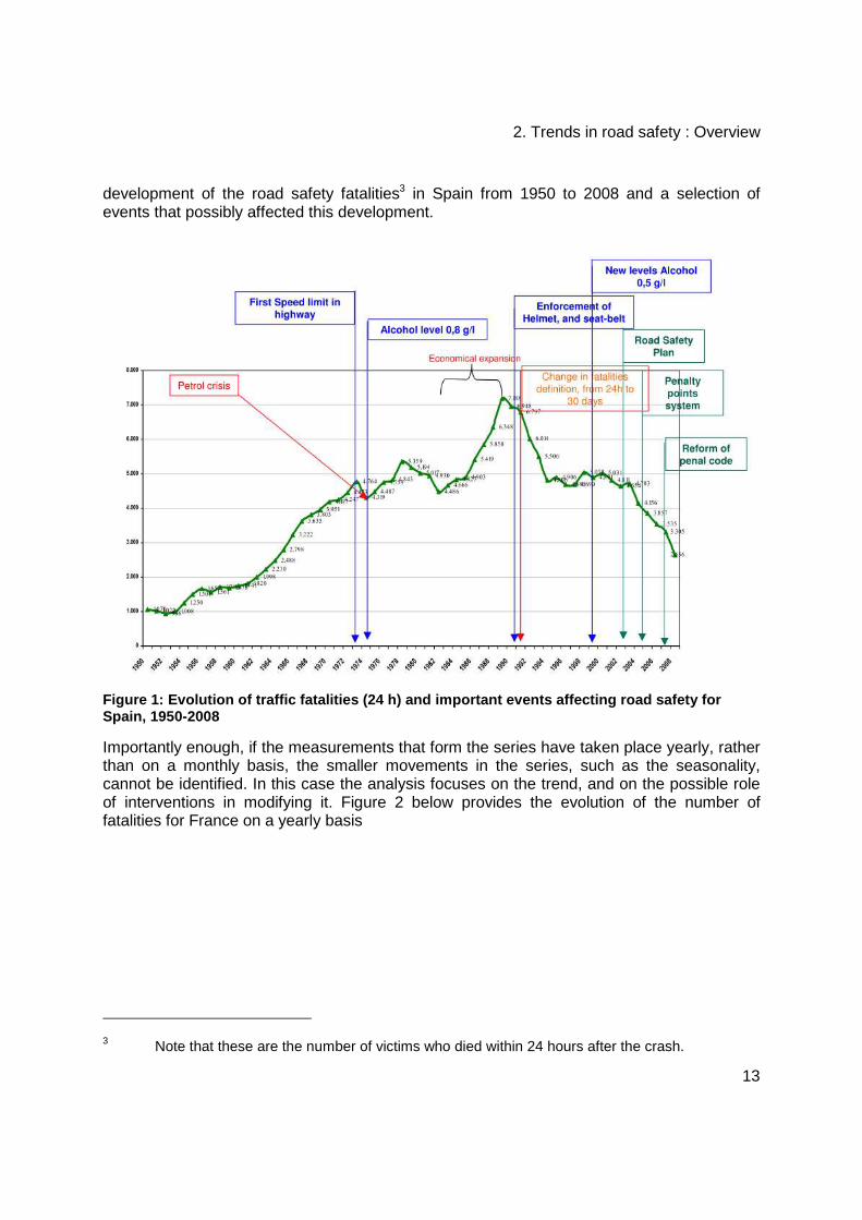
development of the road safety fatalities3 in Spain from 1950 to 2008 and a selection of events that possibly affected this development.
Figure 1: Evolution of traffic fatalities (24 h) an d important events affecting road safety for Spain, 1950-2008
Importantly enough, if the measurements that form the series have taken place yearly, rather than on a monthly basis, the smaller movements in the series, such as the seasonality, cannot be identified. In this case the analysis focuses on the trend, and on the possible role of interventions in modifying it. Figure 2 below provides the evolution of the number of fatalities for France on a yearly basis
3 Note that these are the number of victims who died within 24 hours after the crash.

D4.2: Forecasting traffic fatalities in European countries
14
2.1.2.2.1.2.2.1.2.2.1.2. Risk and exposure as trends:
tues
1960 1965 1970 1975 1980 1985 1990 1995 2000 2005 2010
6000
8000
10000
12000
14000
16000tues
Figure 2. Yearly number of fatalities (30 days) for France.
Whatever the time units of the series, the issue when analyzing them is to extract the trend. Many methods are available, which all aim at identifying the model corresponding to the time function that is as close as possible to the actual development of the observations over time. Another example are the road safety fatalities in France, presented in Figure 2. The trend for France can be considered more as a sequence of local trends than as a general trend: Flat in the fifties, increasing a lot in the sixties up to 1973, then declining sharply at first, and more regularly in the eighties and nineties, ended by a very sharp decrease since 2003. To account for such series, models have to allow the trend to change over time. These models are called dynamic models. Static models, on the opposite, are models where the same trend applies throughout the series. Whether a trend is static or dynamic is important for the precision of forecasts that can be derived from it. The models applied in the analyses performed in Work Package 4 allow to test whether a trend is static or dynamic, and whether interventions lead to significant changes. This way for each country a model can be applied that is best tailored to the dynamic of the trend in question. The exact way trends can be defined by means of those models is further explained in Chapter 3.2.

2. Trends in road safety : Overview
15
2.2. Explaining trends While the occurrence of a single road crahs is always an unpredictable event, the number of crashes or fatalities in a certain period of time in a certain area can be predicted to a certain degree. Moreover, research has identified various factors which make a crash more or less likely to occur.
2.2.1.2.2.1.2.2.1.2.2.1. Heading Factors influencing road safety Road crashes would not occur if people did not use transportation means. It is indeed only to the extent that they are confronted to traffic that individuals run the risk of becoming a traffic victim. A central aim of road safety analysis is to measure and compare the risk of having a crash; measures of exposure to risk are indispensable for providing the context for the crash and casualty data. Risk indicators are generally calculated as the ratios between crash or casualty counts and an appropriate exposure measure. Various indicators exist that quantify more or less satisfactorily the exposure to risk of those travelling by road in a country. They are related more or less directly to the number and type of road crash casualties in that country. The range and detail of indicators that are collected varies between countries (Yannis et al., 2005).
These indicators of exposure are typically divided into three groups: those relating to the people using the roads and their behaviour, those relating to the vehicles being used, and those relating to the road infrastructure. Road safety policies and measures operate upon one or more of these groups.
2.2.1.1.2.2.1.1.2.2.1.1.2.2.1.1. Road users population The characteristics of a country’s population such as the number and age of its residents directly affect the number of casualties. In addition to the obvious demographic factors, there are more subtle behavioural factors: two countries which appear to be similar may have quite different levels of risk because their populations tend to behave differently when travelling by road. These differences can be partly explained by the different national approaches taken to traffic law and enforcement of these laws, but there are also important psychological differences that are difficult to quantify.
All EU member states record details of their populations, so the population size is readily available. It takes no account of the mean distance travelled, however, nor of the people who are exposed abroad, and of foreigners exposed in the country under study .
There are several Performance Indicators related to road user behaviour. For example, the proportion of car occupants who wear seatbelts directly affects the number of casualties in a country, and the proportion of motorcyclists who wear crash helmets is another important indicator (Hakkert et al, 2007; Vis & Van Gent, 2007). Various European countries record a range of these Indicators regularly.
Although traffic law and enforcement undoubtedly influence casualty numbers, there have been relatively few instances where the effects of a new measure on the national casualty trend have been identified beyond dispute. This did occur in Great Britain in 1983, for example, when seat belt wearing was made compulsory for front seat occupants of cars and vans, but only because the wearing rate rose so dramatically that the casualty changes could

D4.2: Forecasting traffic fatalities in European countries
16
be attributed definitely to the measure (see, for example, Harvey and Durbin 1986). In other countries, by contrast, the rate rose more gradually and it has been difficult to separate the effects of the new law from the effects of other changes to the transport system that occurred over the same period.
2.2.1.2.2.2.1.2.2.2.1.2.2.2.1.2. Vehicles fleet The volume of travel on a country’s roads affects the number of road crash casualties, but unfortunately few countries have good statistics about the volume of travel. In other countries, the number of vehicles in the national fleet generally provides a substitute measure, and it is possible to calculate the traffic volume from the number of vehicles and estimates of the annual average distance travelled per vehicle. Crash risk varies with type of vehicle, being especially high for powered two-wheelers, so information by vehicle type is valuable.
Car design has developed to improve crashworthiness over the past two decades, as a result of extensive engineering research. This has played an important part in reducing casualties, although it may be difficult to represent the effect on national casualty trends. One relevant Performance Indicator that has been proposed is the proportion of a country’s car fleet that meets objective safety standards such as the EuroNCAP star rating (Hakkert et al, 2007).
2.2.1.3.2.2.1.3.2.2.1.3.2.2.1.3. Road network In the absence of road user or vehicle exposure data, the length of the road network can also be an indicator of exposure to the risk of having a crash. However, the nature of a country’s road network will affect the number of casualties as well. So if two countries are otherwise similar then the one with the better designed roads will have a lower risk and thus tend to have the fewer casualties. Motorways tend to have the fewer crashes than other roads, relative to the volume of traffic, but the high traffic volumes on motorways can mean that they have relatively many crashes per kilometre of road. Vehicle speeds tend to be higher on rural roads than on urban roads, causing crashes to be more serious, so the degree of urbanisation in a country can influence the national casualty data.
Countries generally have good information about lengths of road, although international comparisons can be complicated by differences in classification. There is far less information, however, about design standards or expenditure on maintenance and construction; furthermore any effects on casualty trends would be lagged.
2.2.1.4.2.2.1.4.2.2.1.4.2.2.1.4. Other factors Several factors that may influence national casualty trends do not fit neatly into any of these groups. Of particular interest at the moment is the influence of economic development as recorded by indices such as the Gross Domestic Product. The economic downturn that began in 2008 in many countries has coincided with widespread fatality reductions; traffic volumes and vehicle sales have certainly fallen, but these direct effects may not explain fully the reductions that have been recorded. The weather is another over-arching factor; however, although many crashes are attributed to adverse weather, the influence of climate upon national casualty trends is likely to prove difficult to establish with yearly data. When applied to monthly data at the regional level, results are still not quite consistent, but when

2. Trends in road safety : Overview
17
correcting for the influence of exposure, rainy months seem to show a higher crash risk than less rainy months (Stipdonk et al., 2008)
2.2.1.5.2.2.1.5.2.2.1.5.2.2.1.5. Relative importance of factors Various exposure indicators have been listed above, and many others can be proposed, but logic and experience suggest that some are more influential than others. Road crashes are an adverse consequence of the use of roads, so traffic volume is probably the principal index: if the national traffic volume were to increase and nothing else were to change then the fact that more people were travelling implies that more would be killed and injured. Note that traffic volume is itself the result of other factors such as population size, number of vehicles, policy and economic activity, so this indicator represents in part the influence of several other factors.
Road safety measures are of particular interest in road safety research. However, it is important to model the general risk trends properly in order to assess their effects reliably. Otherwise, it will be claimed that all measures introduced at a time when risks are reducing overall are effective, and vice versa – which would clearly be wrong. Thus, in spite of the interest attaching to these measures, they should only be introduced into the analysis with care.
This demonstrates the importance of approaching the task of modelling national casualty trends with a coherent strategy, based upon an understanding of the road transport system and the risks that arise for its users. It is not simply a search for “best fit” variables.
2.2.2.2.2.2.2.2.2.2.2.2. Disaggregate trends It is natural to begin the analysis of national casualty trends at the overall (aggregate) level. Results relating to the effectiveness of road safety measures are more likely to be achieved, however, by disaggregate analyses, i.e. analyses of selected groups of casualties. The reason is that most measures affect only a part of the travelling population. For example, if the proportion of motorcyclists who wear helmets increased then fewer motorcyclists would be injured, but the number of injured non-motorcyclists would be unaffected. The increase in the helmet wearing rate could well have an identifiable effect on the number of motorcyclist casualties, yet be impossible to identify if all casualties (i.e. including non-motorcyclists) were analysed.
Thus, in principle it is desirable to divide the totality of road users into groups (Stipdonk et al., 2009). These groups should ideally be reasonably homogeneous, in the sense that individuals within each group tend to face similar types of risk. There are two issues that tend to limit the scope for disaggregation. Firstly, the number of fatalities in each group is inevitably less than the overall number of fatalities, and the increased variability can make it difficult to identify stable trends. Hence, it may be practicable to analyse five groups in a country, but not fifty and certainly not five hundred. Secondly, exposure measures may be available at the overall level but not for each group.
Several types of disaggregation are possible, and the most natural is by road user type. The reason is that, as mentioned above, this disaggregation represents most directly the different types of risk that an individual faces when travelling. For example, the risks faced by two car drivers have far more in common than the risks faced by a car driver and a pedestrian.

D4.2: Forecasting traffic fatalities in European countries
18
The main road user types in Europe are car drivers and passengers, motorcyclists, pedestrians and pedal cyclists. There are several groups of road user with relatively small casualty numbers, such as tractor drivers, and these may well be combined into a single group of ‘others’ for analysis. There are appreciable numbers of injured moped riders in some countries, so it may be worthwhile to have an additional group in these countries.
The main other type of disaggregation is by age and sex, as it is well known that travel choices and crash risk vary with both factors. In addition, age-related physiological changes affect the risk of being injured when involved in a crash. Many countries have experienced appreciable demographic change in recent decades, leading to discussion of the consequences of increasing life expectancy, and this has increased the value of this disaggregation. The main practical problem is to choose a set of age ranges that achieves relatively homogeneous groups yet maintains adequate casualty numbers per group. Also, demographic changes are very slow, so it may well be difficult to identify their effects on casualty trends; it may be more effective to analyse casualty rates per head of population.
While disaggregation by age and sex may be considered as an alternative to disaggregation by road user type, it may be better to disaggregate by both road user type and age/sex. The problems caused by relatively low numbers of fatalities per group probably mean, however, that this would only be possible in countries with relatively large annual fatality totals.
2.2.3.2.2.3.2.2.3.2.2.3. Limits to the possibilities for explanation It is important to recognise that there are limitations to what can be achieved by analysis at the level of national annual totals. Many risk factors can only be assessed by carefully designed analyses of detailed crash data: these factors will influence the national totals, but it is not feasible to measure the influences without digging deeper into the data. As a simple example, consider the effects of darkness. Crash risk is demonstrably greater in the dark than in the daylight, but the hours of daylight and darkness do not change from year to year so the effect on the national totals is constant and cannot be detected.
A technical issue that limits the possibility for explaining trends concerns correlation. If the incidence of two or more factors has developed more or less synchronously over the years then their effects are likely to be correlated. As an example, in a country that experiences a strong economical growth, the mobility usually increases as well. Typically we see an increase in road traffic fatalities in these periods, but a reduction in risk (fatalities per unit of mobility). There are a number of candidate causes for this reduction in risk, like the increased concern with road-safety, the larger budget available for counter measures, the congested roads with slow traffic, the higher share of new – and thus safer – cars. The fact that all these potentially important factors develop in step, can make it difficult if not impossible to identify their effects separately on the national trend.
A more fundamental technical limitation concerns the sheer number of factors that potentially affect national trends. Numerous examples have been mentioned, yet in any country the number of years of casualty data is strictly limited. The casualty counts are also subject to random variation, so it would be unrealistic to expect that more than a handful of statistically significant relationships will be identified between the potential explanatory factors in any particular country and its casualty trends.

2. Trends in road safety : Overview
19
2.2.4.2.2.4.2.2.4.2.2.4. Conclusion The range of factors that potentially influence the casualty trends in a country is wide, but there are limited opportunities for incorporating them in a model of national yearly data. The principal factor is exposure to risk, which makes it possible to check whether the number of fatalities has changed as a result of actual changes in risk or simply as a consequence of changes in traffic volume. The most relevant exposure measure for the number of fatalities is the number of kilometres travelled (either by road users or by vehicles). In the absence of these data, proxies based on fuel sales, the number of vehicles, or possibly the road length can serve as substitute.
2.3. Forecasting trends The objective of the analyses presented in this deliverable is mainly to provide forecasts of road crash fatality numbers in European countries. In the first place it is important to understand what can – and what cannot - be expected from forecasts. Later, we will describe the restrictions that the focus on forecasting puts on the investigation of past developments in a time series.
2.3.1.2.3.1.2.3.1.2.3.1. What are forecasts? Forecasts (resulting from a statistical time series model) consist of projecting into the future trends that are observed in the past. This does not necessarily mean that they will correctly predict what is going to happen. The forecasts are often said to be based on “business as usual”, this means they are based on the assumption that the processes that determined the development in the past will still be at work in the future (e.g., Gorr et al, 2004; Australian Bureau of Statistics, 2009). For road safety, this would mean that those factors that have been discussed in Section 2.2 (e.g., demographic factors, law and enforcement, vehicle fleet and crashworthiness, road-system) keep on exerting the same influence on the number of fatalities and, therefore, that the number of fatalities keeps following the same trend. Under such conditions, we can predict the future number of fatalities in a relatively accurate way.
In practice, there are many reasons why the past development might not be continued. For instance, a new road safety initiative might be the basis for the implementation of a number of new measures, altogether reducing the number of victims at a faster pace than before.
As an example, we can consider the Belgian fatalities. In 2001 there were 1486 fatalities and in the years prior to that, they had been stagnating at that level. After 2001, there was a strong decline in the number of fatalities so that they dropped to +/- 1000 only 4 years later. Such a decline is not predicted by any statistical model based on data up to 2001. In 2001, the first Road Safety Action Plan (Etats Généraux de la Sécurité Routière) was launched, which was accompanied and followed by strong efforts in terms of enforcement, education, and road-engineering. It therefore makes sense to assume that the post- 2001 development differs from that before 2001.
In Figure 3, we present the forecasts that would have been produced in 2001 for the years 2002 to 2010, together with the actual development for those years. One can see that the forecasts clearly overestimate the number of fatalities that were observed in the subsequent years.

D4.2: Forecasting traffic fatalities in European countries
20
Figure 3. Circles: log of yearly number of fataliti es (30 days) for Belgium; full line: forecasts derived from data up to 2001; dashed line: confiden ce interval (95%).
Does this make the model used to produce the forecasts a “bad” model? No, the model made a reasonable prediction given the development of the years preceding 2001. One has to be aware of the fact that forecasts from time series analysis are no crystal ball. They do not allow us to see the future. It just gives an educated guess about the future that is derived from what happened in the past. And if the development of the future does not follow the same rules as the past, such an educated guess can be completely wrong.
The fact that forecasts based on past road safety data can go wrong has been criticized recently by Elvik (2010) and Hauer (2010) who challenged the whole activity of predicting road safety fatalities. For that reason we emphasize here that forecasts are based on the assumption that the development continues in the same way as previously. Forecasting is

2. Trends in road safety : Overview
21
useful for target setting. The knowledge of where the present development is going is needed to formulate challenging but yet achievable targets (Broughton & Knowles, 2010).
In their criticism of different forecasting functions, both Hauer (2010) and Elvik (2010) failed to include confidence intervals. To avoid generating unwarranted expectations, we employ structural time series models (see Chapter 3). These models do not only generate forecasts, they also provide information about how informative the past development is for the future. Going back to the Belgian example we can see, for instance, that the model bases its predictions on the stagnation in the years prior to the forecasted period. However, different developments had taken place in earlier years, so that the model “detects” a lot of uncertainty in the development. As a consequence, the confidence interval around the forecasts is very wide. In the next chapter the model employed by WP4 will be described and it will become clear that the model is – in spite of its rather simple input and output – relatively complex. The reason for this is mainly the correct estimation of the confidence intervals. When comparing forecasted and actual developments, it is important to realize that a model for which the actual development lies within the forecasts’ confidence interval has actually made a “correct” prediction.
With respect to the Belgian example, we can see that the actually observed numbers of fatalities are (almost) within the range of the 95% confidence interval of the 2001 forecast, but not quite. This means that given a continuation of the past development after the year 2001, the observed change would have been very unlikely.
To summarize, time series models give us the best guess of the future development, under the assumption that the past development is continued. Moreover, they quantify the uncertainty of our forecasts. To the extent that there has been a clear trend before, the model is “confident” about its predictions. Erratic developments in the past result in forecasts with very wide confidence intervals.
2.3.2.2.3.2.2.3.2.2.3.2. Including factors that affect road safety In Section 2.2 we have seen that a large number of factors affect road safety, or more specifically the number of road-crash fatalities which are forecasted here. Many time series studies have focused on relating the development of those factors to the developments in road safety (for an overview see Hakim, Shefer, & Hakkert, 1991). In fact many results mentioned in Section 2.2 have been investigated in these kinds of studies. This means that one of the major functions of time series research is to explain the developments of the past.
In the present study however, the focus is on forecasting to the future and this objective is to some extent in contradiction with the objective of explaining the past. This is so because the inclusion of explanatory variables to produce forecasts requires future developments of the explanatory variable in question to be known as well. Take the example of the economic situation: Many studies indicated that whenever the economy recesses, the number of fatalities decreases (e.g., Hakim, et al., 1991; Van den Bossche & Wets, 2003; Kopits & Cropper, 2008). This is important to keep in mind when trying to forecast to the future: If we knew how the economy is going to develop further, this would enable us to improve our fatality forecasts. Unfortunately, the future economic development is unknown. Most economic forecasts span 1 or maximal 2 years (e.g., the Economic Outlook published by the

D4.2: Forecasting traffic fatalities in European countries
22
OECD). For this reason forecasting models usually do not contain (m)any explanatory variables.
If an explanatory factor nevertheless has to be included in a forecasting model, there are two different ways to do it, which we will describe subsequently: 1) scenario’s 2) forecasting the explanatory variable in parallel.
2.3.2.1.2.3.2.1.2.3.2.1.2.3.2.1. Scenarios If the relation between an explanatory factor and the variable that needs to be forecasted has been established in the past, different scenarios can be defined for the future development of the explanatory variable. As an example one could generate three different economical scenarios with a variable like the Gross Domestic Product (GDP). The three scenarios could be “remains as is”, “develops towards earlier maximum”, and ‘develops towards earlier minimum”. The GDP values resulting from the scenarios could be used as if they were actually observed, and the relation between the number of fatalities and the GDP observed in the past years would be used to “tune” the fatality forecasts on the basis of these three sets of predicted GDP values.
The number of scenarios should be kept to a minimum, because they can become confusing very quickly. Moreover, the use of scenarios is only worthwhile if a strong relation has been evidenced between the variable for which scenarios are presented and the one(s) for which forecasts have to be produced.
Presently this approach is not pursued. The model framework used here can, however, easily be extended to incorporate scenarios.
2.3.2.2.2.3.2.2.2.3.2.2.2.3.2.2. Modelling explanatory factors in parallel An explanatory variable forms in itself a time series and can be modelled and forecasted together with the road safety fatalities in a bivariate model. This approach is chosen here for exposure, which is – as noted in Section 2.2.1 -- a central concept in road safety research. Just as the number of fatalities, the number of vehicle kilometres can be measured at regular time points. It is then a time series with its own dynamic and random variations (measurement errors principally).
In road safety research, the assumption prevails that the observed trend in the number of fatalities is actually the product of two trends: the one of exposure (e.g.: the number of vehicle kilometres), and the one of risk (estimated as the rate of fatalities per vehicle kilometre). For each kilometre one is moving in traffic, there is a particular risk of becoming the fatal victim of a crash. The latent risk model (Bijleveld et al. 2008), therefore conceptualizes fatalities as the combination of exposure (i.e. mobility) and fatality risk. The product of the total number of kilometres travelled4 and the risk per kilometre yields the number of fatalities (See Section 3.1).
The two variables modelled for each country are therefore the exposure (e.g. kilometres travelled) and the fatality risk (fatalities per kilometres travelled). This way, the past
4 In fact, usually, the risk is calculated per billion kilometres travelled.

2. Trends in road safety : Overview
23
development of the fatalities will be presented as either changes in the exposure or changes in the risk (or both).
The forecasts can be delivered either in terms of risk and exposure, or in terms of fatalities and exposure. In the present document it is chosen to give the forecasts in terms of numbers of fatalities, as this is the measure that is usually addressed in target setting. For each variable, a forecasted value is estimated for the years 2010 to 2020 and a confidence interval is provided.
There are two main advantages to relying on the principles that the number of fatalities is the product of the total number of kilometres travelled and of the risk per kilometre to produce forecasts. First, the confidence interval for the forecasted fatality number automatically takes into account the uncertainty around exposure and the fatality risk. Second, if external forecasts of exposure exist, these can be entered into the model. Instead of forecasting the exposure itself, the model will then use the external exposure forecasts..
In principle, it is possible to model more than two variables in parallel and produce forecasts for each of them. However, when dealing with yearly data, as is the case in the present study, most variables show actually relatively similar developments. When having to estimate a number of similar trends from time series, the forecasts do not improve much while the confidence intervals become wider. Moreover the interpretation becomes difficult as noted above (see Section 2.2.3). To enable a meaningful interpretation and to obtain the best possible forecasts, we include the one most important variable – exposure – into the model and refrain from including additional ones.
2.3.3.2.3.3.2.3.3.2.3.3. Implementation The latent risk time series model (LRT model, Bijleveld, et al., 2008) is tailored to the risk conception of road safety fatalities. It allows modelling fatalities jointly with exposure and it adjusts the confidence intervals for the forecasts to the past developments of these two variables. As yet, the LRT model has not been implemented in a professional software. The first step for producing forecasts for the European countries was therefore to prepare software that allows researchers without too much extra training to apply the LRT model to the data of different countries. This model has now been implemented and is at this moment used by the WP4 partners. In the future, it can be made available to other interested road safety scientists.
2.4. Summary Road safety data are measured at regular intervals of time. This allows us to analyze the number of traffic fatalities and other road safety indicators over time. From the series of observed data, the trend – representing the long term movement in the series – can be extracted. The trend in the number of traffic fatalities can be studied in different ways. Firstly, it can be described or visualized; secondly, one can try to give a possible explanation for its movement(s) and thirdly, forecasts can be prepared by extrapolating trends. Given the dynamic nature of road safety data, so-called dynamic models, allowing the trend to vary over time, are most appropriate in this respect.

D4.2: Forecasting traffic fatalities in European countries
24
Various factors have an influence on road safety and its trend. In addition to the more indirect influence of factors such as the gross domestic product, three classes can be considered, being the road users (e.g., seatbelt wearing rate), the vehicles (e.g. modal split) and the infrastructure (e.g. the share of the road network per type). Policymakers, aiming to increase the level of road safety, can take action on one or several aspects. It can be investigated whether a (certain part of a) decrease in the number of traffic fatalities is attributable to a particular action or intervention. Nevertheless, separating the effects of an action from the effects of other changes to the transport system that occurred around the same period, is difficult. Moreover, one should bear in mind that most actions are targeted at a specific subgroup of the whole travelling population (such as motorcyclists or children), so that their effects do not necessarily show up when analysing all types of casualties altogether. Disaggregate analyses are valuable in this respect. Road users can be divided into groups based on road user type, age and/or sex. A limited number of fatalities in each group as well as increased variability can however limit the identification of stable trends.
The aim of this work package is to produce forecasts for the number of traffic fatalities in each of the European countries. Advanced time series analysis techniques are used for this (see Section 3.1). The idea is that the trend which has been detected based on past data can be projected to the future. Factors related to the road users, the vehicles, the infrastructure and other factors are assumed to keep exerting the same influence on the number of traffic fatalities, resulting in a continuation of the trend.
The trend in the number of traffic fatalities can be considered as the product of two other trends, i.e. the one of exposure (e.g., the number of kilometres travelled) and that of risk (the number of fatalities per kilometres travelled). In order to forecast the number of traffic fatalities, these two variables will be modelled jointly in this study. As mentioned before, exposure is an essential factor in road safety analysis. Although it is possible to include additional factors, this will not be done in the present study as the objective here is to produce forecasts rather than to explain the past.

3. The Latent Risk Time Series model
25
3. THE LATENT RISK TIME SERIES MODEL The results presented in Chapter 5 are based on the Latent Risk Time series Model (LRT), developed by Bijleveld et al. (2008). The Latent Risk Model is a particular case of a more general class of models, named state-space models, or structural time series models. To the difference of other state-space models however, the latent risk model has been designed to explicitly acknowledge a “risk conception” of road safety. It is sustained by a set of principles that need to be explicitly described for the sake of a correct interpretation of the results presented here.
3.1. The risk conception of road safety The level of road safety – conceived of as the number of people killed in road crashes - is a joint function of “the level of dangerousness” of the traffic system or road risk, and of the extent to which individuals are confronted to that risk, namely, the exposure to the risk. This approach, which consists of decomposing the fatality trend into risk and exposure, was first made popular by Oppe (1989, 1991). This decomposition means that two series of observations have to be modelled in parallel in order to analyse the development of road safety: one for the road safety indicator, the other for the exposure indicator (while risk can be deduced from these two). In the models presented here, the number of fatalities is the road safety indicator5. The indicator for exposure will depend on the data availability in the country in question, but will mostly consists of either the number of vehicle kilometres or the size of the vehicle fleet (for further considerations on the indicators chosen see Chapter 4.)
The assumption that “the development of traffic safety is the product of the respective developments of exposure and risk” (Bijleveld, 2008) can be summarised in the following way (Bijleveld, 2008, p. 46):
RiskExposurefatalitiesofNumber
ExposurevolumeTraffic
×==
3.1
The pair of equations in (3.1) represents the LRT6. One can see that both traffic volume and number of fatalities are treated as dependent variables. Traffic volume is modelled as the result of “exposure”. Fatality numbers, on the other hand, are defined as the result of “exposure x risk”. Conceptually, this amounts to acknowledging that what we measure by means of traffic volume and the number of fatalities is nor exposure, nor exposure x risk, but only a function thereof. To state it otherwise: Traffic volume and fatality numbers are
5 The model is also applicable to other road safety outcomes such as the number of crashes, the number of injured persons etc.
6 Actually, the model defined in equation (3.1) represents only one possible version of the LRT, which can be developed further to include, in addition to exposure and the risk to die on the road, the risk of a crash occurrence. Given that this model won’t be applied in the present analyses, this version of the LRT won’t be presented here.

D4.2: Forecasting traffic fatalities in European countries
26
considered to be the manifest counterparts of “exposure”, and “exposure x risk”, which the model defines as latent variables. This becomes clearer in (3.2), where the logarithms of the variables are used (to make the multiplicative model in (3.1) an additive one), and where a random error term is added to the latent variables:
fatalitiesoferrorrandomriskexposurefatalitiesofNumberLog
volumetrafficinerrorrandomexposurevolumeTrafficLog
++=+=
loglog
log 3.2
Because they define the way exposure and risk can be observed, the equations in (3.2) are called the measurement equations.
The latent variables (log (exposure) and log (risk)) are further modelled by means of the state equations. These can be considered as sub-models, which, once inserted in the general model, describe (or explain) the development of the latent variable. It is under their unobserved, or “state” form that the variables investigated can be decomposed into the several components (trend, seasonal, cycles…), that we have already described in Section 2.1.
3.2. Decomposing trends In the following, we describe in more detail how state equations can be formulated to model various types of trends. For the sake of simplicity, we apply this description to the case where only one variable is modelled (in our example, the number of fatalities). One should bear in mind that this approach does not correspond to the LRT, which takes into account two variables (exposure and risk). Section 3.3 describes how fatalities and exposure are simultaneously treated in the LRT model.
Working only with annual numbers of fatalities, we still could follow the rationale according to which “real” number of fatalities cannot be observed directly, and that the observation that we
make thereof is inevitably contaminated with error ( tε ). The “true” development of the fatalities is hence modelled on the basis of the state equations, and then used as “independent” variable in the measurement equation. There, jointly with the measurement error term it describes the observed development of the actual fatality numbers.
Measurement equation:
ttt LatentFatFatalitiesofNumber ε+= .loglog 3.3
State equations:
3. The Latent Risk Time Series model
27
ttt
tttt
LatentFatSlopeLatentFatSlope
LatentFatSlopeLatentFatLevelLatentFatLevel
ζξ
+=++=
−
−−
)(log)(log(
)(log)(log)(log
1
11 3.4
The above formulation allows replacing the state equation in the framework of the measurement equation previously defined for the Latent Risk Model. In the state equations, the level at time point t is defined as the combination of the level and of the slope of the previous time points. The trend – the sum of level and slope – of one timepoint is therefore equal to the level of the next one, and the level is consequently frequently referred to as to “the trend”. To describe the different possible ways of defining a trend in the state equations, however, a more general formulation than the one used in 3.4 is appropriate. In equations 3.5, Yt represents the observations and is defined by the measurement equation within which
tµ represents the state and tε the measurement error. The state tµ is defined in the state equation. Generally speaking, what the state equations do is describe how the latent variable evolves from one time point to the other. In the present case, it corresponds to the trend for the yearly fatalities.
ttt
tttt
ttt
ζνν
ξνµµ
εµY
+=++=
+=
−
−−
1
11 3.5
The state, tµ , thus corresponds to the fatality trend at year t. It is defined by an intercept, or
level 1−tµ (thus the value of the trend for the year before) plus a slope tν -1, which is the
value by which every new time point is incremented (or decremented depending on the slope
sign, which is usually negative in the case of fatality trends). The slope tν thus represents the effect of time on the latent variable. It is defined in a separate equation, so that a random
error term can be added to it as well ( tζ ). These random terms, or disturbances, allow the level and slope coefficients of the trend to vary over time. A coefficient is said to be treated stochastically when it is allowed to vary over time. It is said to be treated deterministically when no disturbance is assigned to it. As mentioned in Chapter 2, models with stochastic state components are called dynamic models, while those with only deterministic components are called static.
The basic formulation presented in (3.5) allows the definition of a rich set of trend models which covers an extensive range of series in a coherent way:
The model presented in 3.5, where both the level and slope terms are allowed to vary over time is referred to as to the local linear trend model: The trend cannot be defined but locally. In Section 2.1 we saw the example of the fatality series for France, with wide variations in its development: the local linear trend model is appropriate for such a case.
If only the level is allowed to vary over time, we have the so-called local level model. This model can be specified without slope as presented in 3.6:

D4.2: Forecasting traffic fatalities in European countries
28
ttt
ttt
ξµµ
εµY
+=+=
−1 3.6
This means that the trend at time point t is made of the same value (which happens to be the one for the previous year, and the years before up to the first year of measurement), but that it “randomly errs” around that value. The trend defined by the local level model is a random walk going up and down around a mean value.
When a slope is specified in the local level model, but treated deterministically, so that the increment (decrement) taking place at each time point remains precisely the same, we have a local level model with drift (slope) presented in 3.7:
1
11
−
−−
=++=
+=
tt
tttt
ttt
µµ
εµY
ννξν
3.7
The trend is in this case a “composite” with a random walk and a deterministic linear trend.
When the level is fixed and the slope is treated stochastically (3.8), we have a “ smooth trend”, in that case the level is fixed and the slope moves around a mean value in a random walk.
ttt
ttt
ttt
ζ
µµ
εµY
+=+=
+=
−
−−
1
11
ννν 3.8
When both the level and slope components are treated deterministically (3.9), we have a fully deterministic linear trend model: in this case, the level and slope values are considered equal to the level and slope values of the preceding time point. As this applies to all time points, this means that the slope and level values are identical for the whole series of observations:
1
11
−
−−
=+=
+=
tt
ttt
ttt
µµ
εµY
ννν 3.9
Going back to the general model (3.5), a negative value of the level disturbance ( tζ ) indicates that the value of the level drops in comparison to the year before. When the slope
is positive there is an increase, which slows down if the slope disturbance ( tζ ) is negative and becomes even steeper when the slope disturbance is positive. If, on the other hand, the slope is negative, there is a decrease. This decrease becomes even steeper when the slope disturbance is negative and it becomes more shallow if the disturbance is positive.

3. The Latent Risk Time Series model
29
The size of the variance of these disturbances indicates the ease with which the level and slope elements vary over time. Large variances indicate that the level and/or slope parameters need to be treated stochastically. Small variances values indicate on the opposite that the series at hand does not warrant a stochastic treatment of the level and slope, and that the model will actually fit the data better if they are treated deterministically.
3.3. The latent risk time series model We have now looked at two characteristics of the LRT model separately. In Section 3.1.1 we discussed the risk conception underlying the joint modeling of fatalities as a risk-trend and an exposure-trend and in Section 3.1.2 we discussed how latent trends can be decomposed into several components, depending on the dynamics of that trend. This was discussed for the simpler example of a model containing fatalities only, the principles apply however to each of the trends in the LRT model as well. Now it is time to put these two aspects together.
Contrary to the fatality model discussed above in Section 3.1.2, the latent risk model contains two measurement equations: one for traffic volume, and one for the fatalities. To each of these measurement equations correspond in addition two state equations:
For traffic volume:
Measurement equation:
ettt ExposureumeTrafficVol ε+= loglog 3.10
State equations:
ettt
etttt
ExposureSlopeExposureSlope
ExposureSlopeExposureLevelExposureLevel
ζ
ξ
+=
++=
−
−−
)(log)(log
)(log)(log)(log
1
11 3.11
For the fatalities:
Measurement equation:
ftttt RiskExposureFatalitiesofNumber ε++= logloglog 3.12
Note that this equation is qualitatively different from the measurement equation for the number of fatalities in Section 3.1 (Equations 3.2): (1) it includes the unobserved exposure component (exposure state), and (2) it does not refer to “latent fatalities” anymore, but to “Risk”. Indeed, once exposure is included in the model, risk can be estimated as: logRiskt = log LatentFatt-log Exposuret
State equations:

D4.2: Forecasting traffic fatalities in European countries
30
rttt
rtttt
RiskSlopeRiskSlope
RiskSlopeRiskLevelRiskLevel
ζ
ξ
+=
++=
−
−−
)(log)(log
)(log)(log)(log
1
11 3.13
3.4. Explanatory variables and interventions In the models presented here, no further explanatory variables apart from exposure were included (see Section 2.3). Nevertheless it is important to understand the mechanisms that allow including explanatory variables because they also apply to the inclusion of interventions into the model. In the following, we briefly describe how explanatory variables are added to the model. Subsequently we will address the interpretation of including interventions (also called break-points) into the model.
The LRT models the observed development of traffic volume and fatalities (the measurement equations) but also of the latent, true values of exposure and fatality risk (state equations). Explanatory variables that are thought to affect either traffic volume or the number of fatalities can be added to the model in three different ways: 1) Into the measurement equation, where it is assumed to explain the observation errors, 2) in the level equation, where it is assumed to explain the level disturbances and 3) in the slope equation, where it is assumed to explain the slope disturbances. An explanatory variable is inserted into the measurement equation if it is thought to have an effect on observation errors (if, for example, one has reasons to suspect that it affected the registration of fatalities or traffic volume). It will be included in the level equation if it is thought to have an effect on the level of fatalities or exposure, and in the slope equation if it is thought to affect the steepness or direction of change.
A special case of explanatory variables are intervention variables. These are variables that are generated to model the effect of a particular event on the series of observations (e.g., the introduction of a law, the beginning of a crisis, a change in counting methods, etc.). Usually, interventions are coded 0 for all time-points prior to the event and 1 for the time-point of the event and those following. Using interventions as explanatory variable allows testing whether a significant change indeed took place at the specified moment.
The intervention is included into the measurement equation, when it is suspected that some change in the series reflects a change in the way it has been measured and not a change in the phenomenon itself. An example is the redefinition of fatalities from “victims who died within 24 hours after the crash” to “victims who died within 30 days after the crash”, as can be seen in the Spanish and Italian results (see Sections 5.4).
The intervention is included into the level equation if it is thought to have caused a permanent reduction in either the fatality risk (e.g., seat-belt law) or in the exposure (e.g. introduction of taxes). A level intervention takes the form of a step: the fatality risk, for example, increases or decreases at the moment of the intervention and it remains at that level afterwards. (Of course this does not mean that after the intervention there should not be any changes in the component in question any more, only that these changes will occur independently of the intervention.)

3. The Latent Risk Time Series model
31
The intervention is included into the slope equation when something is suspected to have caused a change of direction - or steepness - of the development of either fatality risk or exposure. This could, for example, be an increased commitment in a country to road safety improvement, due to which the fatality risk decreases at a faster rate than before.
The selection of “candidates for interventions” should be based on the results of the analyses of the data, as well as on theoretical knowledge. Measurement or level interventions that are implemented “post-hoc” - when the time series show extreme values or changes - reduce the error variance and consequently the confidence interval for the forecasts. This is a good thing when the forecasts are not supposed to take changes of that nature into account.. However, when the reasons for the changes in the past are not really understood, one has to expect that similar changes could happen in the future as well. In the latter case, correcting the models for the past “quirks” by introducing interventions would artificially reduce the confidence intervals for the forecasts. Slope interventions that are introduced when the fatality risk or the exposure show a change of direction take this change out of the slope-variance. This means the change is no longer considered to be accidental, but structural. This has consequences for the forecasts as well. They will go more into the direction of the change that was identified in the slope intervention.
To summarize, the effect of explanatory variables or interventions can be tested by including them into the model. For interventions, it should be carefully considered whether it is adequate to consider a particular change a structural rather than an accidental one.
3.5. Summary With the LRT model (Bijleveld et al. 2008), we have a model that is optimally fit for the objective of producing road safety forecasts.
• It is tailored to the risk conception of road safety fatalities
• It can be tailored to the dynamics of the development of exposure and to the development of risk for the country in question.
• The confidence intervals are based on the estimation of different types of dynamic variances.
• The model can deal with measurement errors and missing observations by means of the latent trend approach.
The model, although complex in itself, can be presented in a relatively simple way. The data requirements, fatalities and some measure of exposure are achievable for the large majority of the European countries.
A problem that had to be overcome in order to be able to use it, is that it is not implemented in any professional software package yet. The first step for producing forecasts for the European countries was therefore to prepare software that allows researchers without too much training to apply the LRT model to the data of different countries. To achieve this, the model has been implemented as a module that can be called for by the statistical free-ware “R”. R has become the standard software in many scientific disciplines as it is open to extensions from different fields of analysis. It is supported by a large group of experts all over

D4.2: Forecasting traffic fatalities in European countries
32
the world, can be downloaded for free, and runs on the different platforms in use (Windows, MAC, Linnux, Unix…).
The module produced by Frits Bijleveld for DaCoTA, Workpackage 4 is still in the test phase and not yet public. It is built around a procedure (“fitDaCoTAModel”). The procedure allows estimating the trend and slope for the LRT model described here. Explanatory variables and interventions can be included at the different levels as described in Section 3..4. It also allows including additional levels (i.e., dependent variables, such as for example the number of crashes), and/or splitting up the fatalities and/or the exposure into subgroups (e.g. per road-user type as suggested in Section 2.2.2), so as to model them jointly. The module produces the usual tests of model adequacy (see e.g., Commandeur & Koopman, 2007) and of course the forecasts and confidence intervals. The output can be produced under the form of both tables and graphs. To summarize: The module does what other time series packages do as well (e.g. STAMP), but includes the road safety specific LRT model, which is not available in other packages.
Bijleveld’s module can be made available to road safety scientists who would want to update the forecasts for their countries in future years. The input is code rather than menu-based, but should be accessible thanks to the manual (Bijleveld et al., in preparation), the instruction (see Appendix B3 for a preliminary version), and the examples produced in WP4.

4. Data Availability
33
4. DATA AVAILABILITY In this chapter, the availability of data for implementing the LRT model proposed in Chapter 3 is addressed. As mentioned there, in the LRT model a measure of road (un)safety is modelled jointly with a measure of exposure. However, the choice of an appropriate indicator - be it for “road safety” or for “exposure” - is never straightforward. There is, of course, no one measurable variable that would be an ideal, exhaustive indicator for something as “the level of road safety in a country”. The choice made here is based for a part on pragmatic considerations, such as data availability and reliability. As a consequence, the “road safety indicator” that is eventually selected provides only a partial reflection of the road safety situation. The analyses to be produced in WP4 have to apply to most countries of the European Union. The models to be used could consequently not be too demanding in terms of data, while allowing the description of past trends and the production of forecasts. For this reason, annual fatality numbers were selected as road safety indicator. We will see below that this variable is available in most member states for a sufficient period of time, and it is also known to be one of the most reliably measured (compared with the number of injuries, for example).
As far as exposure is concerned, no single indicator can be selected. The preferred indicator for the purpose of the present analysis is the annual number of vehicle kilometres (Yannis et al., 2005). Some countries, however, do not register vehicle kilometres. It was thus necessary to define alternative exposure indicators. The vehicle fleet, i.e. the total number of motorised vehicles in a country has been selected as the second most appropriate exposure indicator. Oil sales form the back-up indicator.
For the fatality data, the CARE database is examined with respect to the number of countries that have a series of yearly fatality numbers published there. For exposure data those stored in the Eurostat databases are considered. For the model proposed here a time series that includes 15 years is sufficient although more years are preferable. In the present investigation of data availability, the start year of the CARE database (1991) is selected as a starting point, based on the assumption that countries that have data back to 1991 qualify for the implementation of the model.In several cases longer series are available, for example from national data sources, which will eventually be used for the modelling. The information presented in this chapter is initially collected and cross-checked by DaCoTA WP3 - Data Warehouse.
4.1. Fatality data Table 1 shows the availability of fatality data by country and by year in the CARE database, for the 27 EU Member States, plus Switzerland. It can be seen that older Member States, namely the EU-15 have fatality data that span the entire period 1991-2008. On the other hand, data availability for the new Member States is limited to a small number of recent years (e.g. from 2005 onwards for Estonia and Slovakia, from 2003 onwards for Hungary, from 2000 onwards for Slovenia etc.). Longer series for the overall number of fatalities should be however available at national level.

D4.2: Forecasting traffic fatalities in European countries
34
Countries /Year 1991 1992 1993 1994 1995 1996 1997 1998 1999 2000 2001 2002 2003 2004 2005 2006 2007 2008
Belgium • • • • • • • • • • • • • • • • • •Czech Republic • • • • • • • • • • • • • • •Denmark • • • • • • • • • • • • • • • • • •Germany • • • • • • • • •Estonia • • • •Ireland • • • • • • • • • • • • • • • • • •Greece • • • • • • • • • • • • • • • • • •Spain • • • • • • • • • • • • • • • • • •France • • • • • • • • • • • • • • • • • •Italy • • • • • • • • • • • • • • • • • •Cyprus •Latvia • • •Luxembourg • • • • • • • • • • • • • • • • • •Hungary • • • • • •Malta • • • •Netherlands • • • • • • • • • • • • • • • • • •Austria • • • • • • • • • • • • • • • • • •Poland • • • • • • • •Portugal • • • • • • • • • • • • • • • • • •Romania • • • • • • • • • •Slovenia • • • • • • • • •Slovakia • • • •Finland • • • • • • • • • • • • • • • • • •Sweden • • • • • • • • • • • • • • • • • •United Kingdom • • • • • • • • • • • • • • • • • •Switzerland •Source: CARE
Date of query: November 2010
Table 1: Fatality data availability by country a nd by year 1991-2008
It is reminded that the CARE database includes harmonised fatality data, which conform to the European definition of fatalities within 30 days from the crash. This should be kept in mind when collecting data from other sources at national level, in order to complete the time series (i.e. a common definition should be applied for the entire period examined).
4.2. Exposure data The exposure indicators examined include the number of vehicle-kilometres of travel, the vehicle fleet, the fuel consumption and the road length. If possible, a common definition should be applied for the entire period examined. Alternatively a change in measurement or definition can be implemented in the model as an intervention (see, e.g., the results for Italy in Section 5.4 and in Appendix Section 4).
4.2.1.4.2.1.4.2.1.4.2.1. Vehicle kilometres Table 2 presents the data availability concerning vehicle kilometres of travel in the Eurostat database, as determined by DaCoTA WP3. It can be seen that vehicle kilometres data is available for a sufficient number of years only for a limited number of countries, namely: Germany, France, Netherlands, Finland, Sweden, the UK, Norway and Switzerland. For the remaining countries, the series are largely incomplete. A few countries have vehicle-kilometres data for ten consecutive years (e.g. Portugal, Latvia).
Consequently, ,it is unlikely that the proposed analysis can be carried out on the basis of vehicle-kilometres data for the majority of European countries. Alternative exposure indicators need to be examined in each case.

4. Data Availability
35
Countries /Year 1991 1992 1993 1994 1995 1996 1997 1998 1999 2000 2001 2002 2003 2004 2005 2006 2007 2008
Belgium • • • • • • • •Bulgaria • • • • • • • • •Czech Republic • • • • • • • • • • • •Denmark • • • • • • • • • • •Germany • • • • • •Estonia • • • • • • • • • • • •Ireland • • • • • •Spain • • • • •France • • • • • • • • • • • • • • • • •Italy • •Cyprus •Latvia • • • • • • • • • • • •Lithuania • • • • • • • • • • • • • • • • •Luxembourg • • • • • •Netherlands • • • • • • • • • • • • •Austria • • • • • • • •Poland • • • • • • • • • • • • • • • •Portugal • • • • • • • • • • • • •Romania • • •Slovakia • • • • • • • • • • • • • •Slovenia • • • • • • • • • • • • • • • • • •Finland • • • • • • • • • • • • • • • • • •Sweden • • • • • • • • • • • • • • • • • •United Kingdom • • • • • • • • • • • • • • • • • •Norway • • • • • • • • • • • • • •Switzerland • • • • • • • • • • • • •Source: Eurostat (Dacota 3.2.2 Assembly of risk exposure data)
Date of query: June 2010
Table 2: Vehicle kilometres data availability by country and by year 1991-2008
4.2.2.4.2.2.4.2.2.4.2.2. Vehicle Fleet Table 3 presents the data availability by country and by year with respect to vehicle fleet, including lorries, road tractors, passenger cars, motor coaches, buses and trolley buses, special vehicles, total utility vehicles, but not including trailers and motorcycles. The complete series is available for 14 countries, whereas for the remaining ones the data are quite incomplete.
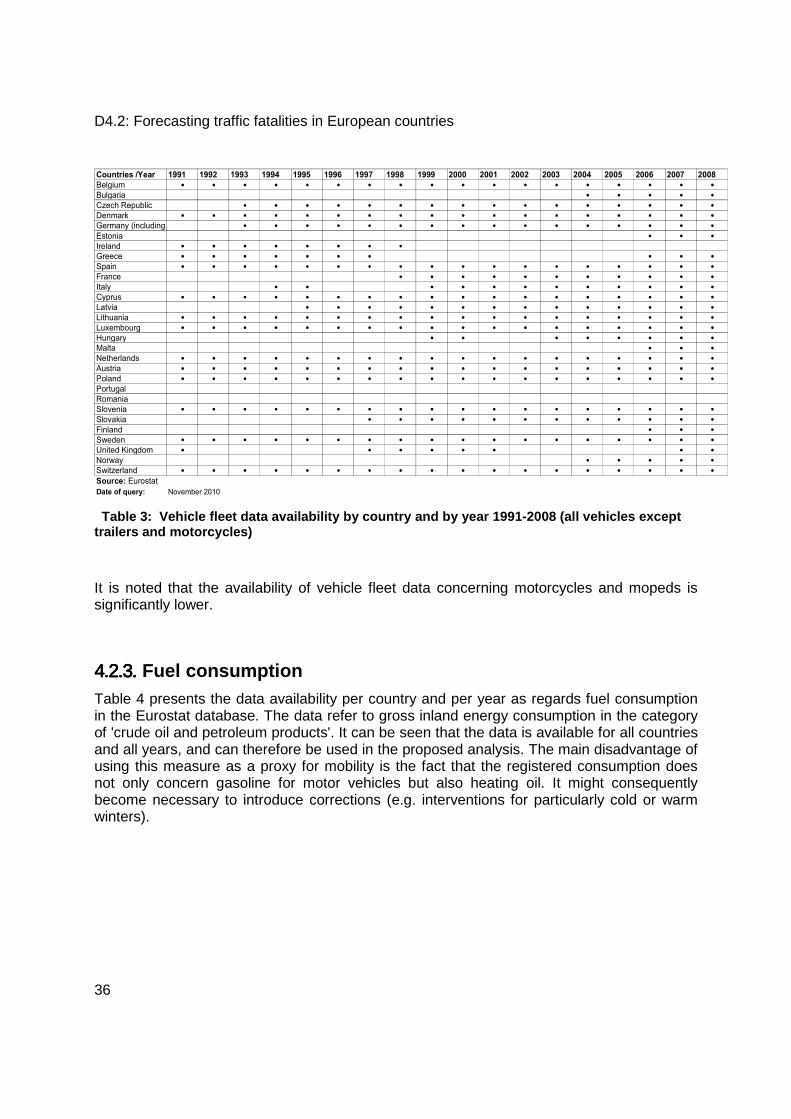
D4.2: Forecasting traffic fatalities in European countries
36
Countries /Year 1991 1992 1993 1994 1995 1996 1997 1998 1999 2000 2001 2002 2003 2004 2005 2006 2007 2008
Belgium • • • • • • • • • • • • • • • • • •Bulgaria • • • • •Czech Republic • • • • • • • • • • • • • • • •Denmark • • • • • • • • • • • • • • • • • •Germany (including • • • • • • • • • • • • • • • •Estonia • • •Ireland • • • • • • • •Greece • • • • • • • • • •Spain • • • • • • • • • • • • • • • • • •France • • • • • • • • • • •Italy • • • • • • • • • • • •Cyprus • • • • • • • • • • • • • • • • • •Latvia • • • • • • • • • • • • • •Lithuania • • • • • • • • • • • • • • • • • •Luxembourg • • • • • • • • • • • • • • • • • •Hungary • • • • • • • •Malta • • •Netherlands • • • • • • • • • • • • • • • • • •Austria • • • • • • • • • • • • • • • • • •Poland • • • • • • • • • • • • • • • • • •Portugal
Romania
Slovenia • • • • • • • • • • • • • • • • • •Slovakia • • • • • • • • • • • •Finland • • •Sweden • • • • • • • • • • • • • • • • • •United Kingdom • • • • • • • •Norway • • • • •Switzerland • • • • • • • • • • • • • • • • • •Source: Eurostat
Date of query: November 2010
Table 3: Vehicle fleet data availability by coun try and by year 1991-2008 (all vehicles except trailers and motorcycles)
It is noted that the availability of vehicle fleet data concerning motorcycles and mopeds is significantly lower.
4.2.3.4.2.3.4.2.3.4.2.3. Fuel consumption Table 4 presents the data availability per country and per year as regards fuel consumption in the Eurostat database. The data refer to gross inland energy consumption in the category of 'crude oil and petroleum products'. It can be seen that the data is available for all countries and all years, and can therefore be used in the proposed analysis. The main disadvantage of using this measure as a proxy for mobility is the fact that the registered consumption does not only concern gasoline for motor vehicles but also heating oil. It might consequently become necessary to introduce corrections (e.g. interventions for particularly cold or warm winters).

4. Data Availability
37
Countries /Year 1991 1992 1993 1994 1995 1996 1997 1998 1999 2000 2001 2002 2003 2004 2005 2006 2007 2008
Belgium • • • • • • • • • • • • • • • • • •Bulgaria • • • • • • • • • • • • • • • • • •Czech Republic • • • • • • • • • • • • • • • • • •Denmark • • • • • • • • • • • • • • • • • •Germany • • • • • • • • • • • • • • • • • •Estonia • • • • • • • • • • • • • • • • • •Ireland • • • • • • • • • • • • • • • • • •Greece • • • • • • • • • • • • • • • • • •Spain • • • • • • • • • • • • • • • • • •France • • • • • • • • • • • • • • • • • •Italy • • • • • • • • • • • • • • • • • •Cyprus • • • • • • • • • • • • • • • • • •Latvia • • • • • • • • • • • • • • • • • •Lithuania • • • • • • • • • • • • • • • • • •Luxembourg • • • • • • • • • • • • • • • • • •Hungary • • • • • • • • • • • • • • • • • •Malta • • • • • • • • • • • • • • • • • •Netherlands • • • • • • • • • • • • • • • • • •Austria • • • • • • • • • • • • • • • • • •Poland • • • • • • • • • • • • • • • • • •Portugal • • • • • • • • • • • • • • • • • •Romania • • • • • • • • • • • • • • • • • •Slovenia • • • • • • • • • • • • • • • • • •Slovakia • • • • • • • • • • • • • • • • • •Finland • • • • • • • • • • • • • • • • • •Sweden • • • • • • • • • • • • • • • • • •United Kingdom • • • • • • • • • • • • • • • • • •Iceland • • • • • • • • • • • • • • • •Norway • • • • • • • • • • • • • • • • • •Switzerland • • • • • • • • • • • • • • • • • •Source of Data:: Eurostat
Last update: 11.11.2010
Hyperlink to the table:http://epp.eurostat.ec.europa.eu/tgm/table.do?tab=table&init=1&plugin=1&language=en&pcode=tsdcc320
Date of query: November 2010
Table 4: Fuel consumption data availability by c ountry and by year 1991-2008
4.2.4.4.2.4.4.2.4.4.2.4. Road length Table 5 presents the availability of road length data for motorways for the European countries. The data is available for almost all countries for the entire period examined.

D4.2: Forecasting traffic fatalities in European countries
38
Countries /Year 1991 1992 1993 1994 1995 1996 1997 1998 1999 2000 2001 2002 2003 2004 2005 2006 2007 2008
Belgium • • • • • • • • • • • • • • • • •Bulgaria • • • • • • • • • • • • •Czech Republic • • • • • • • • • • • • • • • • • •Denmark • • • • • • • • • • • • •Germany • • • • • • • • • • • • • • • • • •Estonia • • • • • • • • • • • • • • • • • •Ireland • • • • • • • • • • • • • • • •Greece • •Spain • • • • • • • • • • • • • • • • • •France • • • • • • • • • • • • • • • • •Italy • • • • • • • • • • • • • • • • •Cyprus • • • • • • • • • • • • • • • • •Latvia
Lithuania • • • • • • • • • • • • • • • • • •Luxembourg • • • • • • • • • • • • • • •Hungary • • • • • • • • • • • • • • • • •Netherlands • • • • • • • • • • • • • •Austria • • • • • • • • • • • • • • • • • •Poland • • • • • • • • • • • • • • • • • •Portugal • • • • • • • • • • • • • •Romania • • • • • • • • • • • • • • • • •Slovenia • • • • • • • • • • • • • • • • • •Slovakia • • • • • • • • • • • • • • • • • •Finland • • • • • • • • • • • • • • • • • •Sweden • • • • • • • • • • • • • • • • • •United Kingdom • • • • • • • • • • • • • • • • • •Norway • • • • • • • • • • • • • •Switzerland • • • • • • • • • • • • • •Source: Eurostat
Date of query: November 2010
Table 5: Road length data availability by countr y and by year 1991-2008 - Motorways
Table 6, on the other hand, presents the availability of road length data for other roads (state, provincial, communal) for the European countries. Again, the data is available for a satisfactory number of countries, although the series are generally less complete compared to those of motorway length.

4. Data Availability
39
Countries /Year 1991 1992 1993 1994 1995 1996 1997 1998 1999 2000 2001 2002 2003 2004 2005 2006 2007 2008
Belgium • • • • • • • • • • • • • • • • • •Bulgaria • • • • • • • • • • • • • • • • • •Czech Republic • • • • • • • • • • • • • • • • • •Denmark • • • • • • • • • • • • •Germany (including
Estonia • • • • • • • • • • • • • • • • • •Ireland • • • • • • • • • • • • • • • •Greece • • • •Spain • • • • • • • • • • • • • • • • • •France • • • • • • • • • • • • • • • •Italy • • • • • • • • • • • • • • •Cyprus • • • • • • • • • • • • • • • • •Latvia • • • • • • • • • • • • • • • • • •Lithuania • • • • • • • • • • • • • • • • •Luxembourg (Grand-Duché)• • • • • • • • • • • • • • •Hungary • • • • • • • • • • • • •Malta • • • • • • •Netherlands • • • • • • • • • • •Austria • • • • • • • • • • • • • • • •Poland • • • • • • • • • • • • • • • • • •Portugal • • • • •Romania • • • • • • • • • • • • • • • • •Slovenia • • • • • • • • • • •Slovakia • • • • • • • • • • • • • • • • • •Finland • • • • • • • • • • • • • • • • • •Sweden • • • • • • • • • • • • • • • • • •United Kingdom • • • • • • • • • • • • • • • • • •Norway • • • • • • • • • • • • • • •Switzerland • • • • • • • • • •Source: Eurostat
Date of query: November 2010
Table 6: Road length data availability by countr y and by year 1991-2008 - Other roads (state, provincial, communal)
4.3. Summary Overall, the availability of fatality data is quite satisfactory, given that the complete series 1991-2008 is available for more than half of the European countries, whereas data for even more countries should be available and can be collected from national sources. It is noted that improved availability is observed in the older EU member states. Consequently, the potential for implementing the proposed time series analysis largely depends on the availability of exposure data.
In particular, complete series of vehicle kilometres data and vehicle fleet data are available for around 15 European countries. The same imbalance within the EU is observed as for fatalities, given that data availability mainly concerns the older Member States. Nevertheless, partially complete series of vehicle fleet data are available for several other European countries.
Road length data is more often available (in more countries and for larger number of years), especially with respect to motorways. Therefore, this can be a useful alternative exposure measure in the proposed analysis.
Finally, as regards fuel consumption, all the necessary data appears to be available in the Eurostat databases. However, the suitability of this data as exposure measure may be an issue for further discussion.
From the above analysis it appears that the basic time series model for fatalities can be applied for all European countries, provided that additional data may be collected from

D4.2: Forecasting traffic fatalities in European countries
40
national sources as well. It is further estimated that for the majority of the countries either an estimated number of vehicle kilometres or the size of the vehicle fleet is available for the majority of the countries. For a few countries, oil consumption will have to serve as a proxy for mobility.
As regards more disaggregate analyses, e.g. per road user type, age group etc., these are even more dependent on the availability of disaggregate exposure data per road user type, age group etc., which is currently not available at Eurostat. Such data may be available at national level for a very limited number of countries. Other disaggregations - e.g. per vehicle type and road type may be more promising as regards the availability of exposure data at disaggregate level, as these can be already found at the Eurostat database.

5. Preliminary Results
41
5. PRELIMINARY RESULTS The methodology developed here has so far been applied to the following countries: Belgium, Spain, Greece, and Italy, and United Kingdom. The extended reports on the results are included in the Appendix A. The instructions for the analyses are presented in Appendix B.
5.1. Belgium
5.1.1.5.1.1.5.1.1.5.1.1. Data
Figure 4: Traffic volume (vehicle kilometres) for Belgium, 1973 to 2009; total number of observations in the series: 37)
Figure 5: Fatalities (30 days) for Belgium: 1973 to 2009; total number of observations in the series: 37. Note: number for 2009 estimated on the basis of fatalities on the spot.
The registration of traffic fatalities is based upon forms that are in use since 1991 (before there were other forms). The latest official number of victims killed on the spot in a crash or within 30 days after the crash concerns the year 2008. For 2009 an estimation is used, based on the number of fatalities on the spot.
The number of vehicle kilometres is estimated yearly on the basis of traffic counts and road lengths. The method presently employed has been introduced in 1985, which is the start of the series that has been taken into account for the forecast7.
7 Preliminary analyses have been conducted on the series starting in 1973, but it revealed problems with the pre-1985 exposure data violating assumptions that must be satisfied to get reliable results.

D4.2: Forecasting traffic fatalities in European countries
42
The general trend in the Belgian fatalities is decreasing. However, the decrease is not a stable one. From 1985 to 1989, at the beginning of the period studied here, the number of fatalities was increasing and the same is true between 1996 and 2001.
5.1.2.5.1.2.5.1.2.5.1.2. Breakpoints FL1991 - In 1991 regulations improved the position of vulnerable road users in traffic, and seat-belts became mandatory in the back-seats. Moreover, the registration of crashes was changed in 1991, as the presently used forms were introduced then, (although initially they were filled in on paper). In 1991 we see a drop in the fatalities. In the model, this results in a significant breakpoint in the fatality risk.
FS2001 - 2001 is a year where many changes took place. First, the registration was changed: a computerized version of the crash registration form is used since then. This probably made a difference in terms of “lost forms”. Second, the whole Belgian police system was reformed at that time, and this may temporarily have given crash registration a lower priority. At the same time however, the statistical office paid more attention to the issue of missing crash forms for fatal victims (as registered by the hospitals). From 2002 on, these fatal victims for whom there was no crash form were included in the fatality counts. In 2001 a working group was founded by the Belgian Road Safety Institute, with the aim of tracing the fatalities for which no crash form had been sent back to the police departments, resulting in a strong decrease in the number of non-registered fatal victims. Moreover, in 2001, the first Road Safety Action Plan (Etats Généraux de la Sécurité Routière) was launched, which was accompanied and followed by strong efforts in terms of enforcement, education, and road-engineering. For all these reasons, 2001 certainly qualifies for a breakpoint. It is important to realize that the improved registration and the measures that took place has had opposed effects in the number of recorded fatalities. The decrease that we observe is probably an underestimation of the true decrease, because the registration of fatal crashes was improved at the same moment.
The change in 2001 was not so much a drop in the fatalities, than a change of direction in the development. Statistically speaking, this change of direction is only just significant, which makes it difficult to decide whether it should be considered a structural change or just random variation. The assumption of a structural change leads to lower forecasted fatality numbers in the following years than the assumption that the post-2001 decrease was just due to random variation. Given that the forecasts will form the basis for target setting, they are based on the more ambitious model, which assumes that a structural change took place after launching the road safety action plan.

5. Preliminary Results
43
5.1.3.5.1.3.5.1.3.5.1.3. Development of exposure and risk
Figure 6: Exposure (based on Vehicle kms) and risk (fatalities per 109 vehicle kms) for Belgium.
The model run to generate the output presented here was an LRT model with stochastic (random) levels and slopes for exposure and fatality risk (see Model 2.4 in Tables A4 and A5 for more details.) The trends (level + slope) for each variable are depicted in Figure 6. In the trend of the fatality risk, we can see that for those periods where the number of fatalities actually increased (mid-80s and mid 90s) the fatality risk was stagnating but not increasing. This means that a stronger increase in traffic volume together with a stagnating risk was responsible for these two periods of increasing fatality numbers.
5.1.4.5.1.4.5.1.4.5.1.4. Forecasts

D4.2: Forecasting traffic fatalities in European countries
44
Figure 7: Forecast plots for Belgium ( Model 2.4): Left graph:traffic volume, right graph: fatalities
Traffic volume
(vehicle kms per million) Fatalities
Year Estimated
value Lower limit
Upper limit
Estimated number
Lower limit Upper limit
2010 98666 96410 100975 880 779 995 2011 98990 95450 102661 836 705 992 2012 99315 94473 104405 794 642 983 2013 99641 93430 106265 755 586 971 2014 99968 92311 108259 717 536 958 2015 100296 91119 110397 681 491 944 2016 100625 89857 112684 647 450 930 2017 100956 88532 115123 614 412 915 2018 101287 87149 117719 584 378 901 2019 101620 85714 120477 554 347 886 2020 101953 84233 123401 527 318 871 Table 7: Forecasts for Belgium - The upper and the lower limit define the confidence interval in which the values lie with 95% chance if the present trend is continued.
5.2. Spain
5.2.1.5.2.1.5.2.1.5.2.1. Data

5. Preliminary Results
45
Figure 8: Traffic volume (vehicle kilometres) for Spain 1961 to 2008; total number of observations in the series: 48)
Figure 9: Fatalities (24h for Spain 1961 to 2008; total number of observations in the series: 48)
The registration of the Spanish traffic fatalities is based upon forms filled in by the police. There have been changes in the way of registration along the period of study, but we believe that it did not influence the reported number of fatalities. In 1993, the new definition of fatalities was adopted. This new definition includes fatalities up to 30 days after a crash, but in the series studied we only included fatalities at 24h for all the period 1961-2009.
The number of vehicle-kms is estimated and includes only non-urban trips. The quality of this estimate is unknown. From 1994, there is a change in the way of calculation, but it seems that it does not cause a break in the series.
As there are no breaks for the fatalities and vehicle kilometres series related to reporting issues, no intervention variables have been included in the models for adjustment.
5.2.2.5.2.2.5.2.2.5.2.2. Breakpoints There have been a number of events and measures since 1961 that could have affected the number of fatalities and the exposure. We describe those that have been found significant in the models:
1973: In 1973 there was an oil crisis that began on October 17, which resulted in an increase of oil prices. The prices increase coupled with the heavy reliance of the industrialized world on OPEC oil, triggered a strong inflationary effect and reduced economic activity in the affected countries.
Regarding road safety interventions in 1973, the limit of alcohol was established at 0,8g/l and in 1974 the first speed limit was established for highways (130km/h). In Spain, we can see a decrease in 1973 in the number of fatalities and in the number of vehicle kilometres. In the model this is considered by means of a level and slope interventions on the exposure in 1973. The slope intervention was significant and corresponds to a change of direction in the evolution of exposure (i.e. a reduction instead of an increase).
1984: In the mid eighties there is a period of economical expansion. The number of fatalities shows a large increase. It is included in the model as an intervention in the slope for exposure..
1989: After a long period of economical expansion, at the end of the eighties and early nineties there is a period of economic recession. Regarding road safety interventions in 1989 the number of fines increased. 1989 is the year with the maximum number of fatalities along the period, from which there is an inflection and a change in the slope which starts to decrease. It is included in the model as an intervention in the level and slope of the fatality risk.
1994: The economy started to recover from the recession in the middle nineties. In 1992, new road safety measures were implemented. These included the enforcement of helmet for motorised 2-wheelers and of seat-belt for the front car seats. The safety of the Spanish

D4.2: Forecasting traffic fatalities in European countries
46
vehicle fleet started to improve. The number of fatalities from 1994 changes from the previously decreasing slope to a stagnating one until 2003. It is included in the model as an intervention as fatality risk slope.
2007: In June 2006, the Penalty Points System was implemented and in December a Reform of the Penal Code took place that resulted in the increase of the penalties for traffic violations (prison penalties were also foreseen). The number of fatalities decreased sharply. It is included in the model as interventions for the exposure level and slope.
5.2.3.5.2.3.5.2.3.5.2.3. Development of exposure and risk
Figure 10: Exposure (based on Vehicle kms) and risk (fatalities per 109 vehicle kms) for Spain.
The model run to generate the output presented here was an LRT model with stochastic (random) slopes and fixed levels for exposure as well as fatality risk (see Model 3.4 in Table A8 and A9 for details). The trends (level + slope) for each variable are depicted in Figure 10. For the initial period where the number of fatalities increased (1961-1982) the fatality risk was decreasing. This means that a stronger increase in traffic volume was actually responsible for this increasing fatality numbers. As the increase in traffic volume has exceeded the increase in number of fatalities, in terms of risk there has been a reduction over the period. In the middle of this period there is stagnation in the decrease of risk, because the oil crisis of 1973 has reduced the traffic volume while the number of fatalities continued to rise. In contrast, the sharp increase in the number of fatalities in the 1985-1989 period has resulted from an increased risk in this period, because the increase in traffic volume has been proportionately less than the number of deaths. This period coincides with the country's economic expansion from 1984. Another remarkable period is the 1990-1994, where there was a sharp decrease in the number of fatalities even though the traffic volume continued to rise despite the onset of the crisis of 90, and therefore there is a strong risk reduction. Another period to stress in our series is the 1994-2003 which coincides with the beginning of a new situation of economical expansion which stabilizes the number of deaths even though the traffic volume continues to rise, representing a risk reduction. Finally, the

5. Preliminary Results
47
last period 2004-2007, where road safety has been incorporated into the political agenda as a priority, there was a sharp decrease in the number of deaths. As it was accompanied by a slowdown in the traffic volume the resulting risk reduction was however less pronounced. This is also reflected in the fact that the intervention of around 2003 has not been significant in the final model.
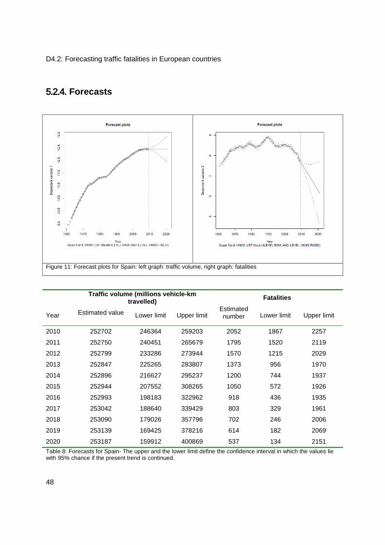
D4.2: Forecasting traffic fatalities in European countries
48
5.2.4.5.2.4.5.2.4.5.2.4. Forecasts
Figure 11: Forecast plots for Spain: left graph: traffic volume, right graph: fatalities
Traffic volume (millions vehicle-km travelled) Fatalities
Year Estimated value Lower limit Upper limit Estimated number Lower limit Upper limit
2010 252702 246364 259203 2052 1867 2257
2011 252750 240451 265679 1795 1520 2119
2012 252799 233286 273944 1570 1215 2029
2013 252847 225265 283807 1373 956 1970
2014 252896 216627 295237 1200 744 1937
2015 252944 207552 308265 1050 572 1926
2016 252993 198183 322962 918 436 1935
2017 253042 188640 339429 803 329 1961
2018 253090 179026 357796 702 246 2006
2019 253139 169425 378216 614 182 2069
2020 253187 159912 400869 537 134 2151
Table 8: Forecasts for Spain- The upper and the lower limit define the confidence interval in which the values lie with 95% chance if the present trend is continued.

5. Preliminary Results
49
5.3. Greece
5.3.1.5.3.1.5.3.1.5.3.1. Data
Figure 12: Traffic volume (number of vehicles (per 1000) in circulation for Greece from 1960 to 2008; total number of observations in the series: 49)
Figure 13: Fatalities (30 days, for Greece from 1960 to 2008; total number of observations in the series: 49)
Before 1996 road crash fatalities in Greece were recorded based on the 24-hour definition, while since then the 30-day definition is used. The data presented in Figure 13 above correspond to the 30-day definition for the entire period, converted via appropriate factors for the period prior to 1996. The latest year for which official data were available for this analysis is 2008.
There are no vehicle kilometre data for Greece and therefore the vehicle fleet is used as a proxy. A clear increasing trend is observable in the number of vehicles in circulation.
The presented fatality data for Greece show two distinct trends: an increasing one until 1995, followed by a decreasing one thereafter. As there are only 12 data points describing the decreasing trend, it is expected that reserving a large number of observations for forecasting may affect the accuracy of the model.
5.3.2.5.3.2.5.3.2.5.3.2. Breakpoints There are three main events that can be entered as interventions in the model for the period and data that are being analysed:
1986: in 1986 Greece encountered a financial crisis, which affected mobility and therefore exposure (note that –due to lack of the data- the exposure variable in the Greek dataset is vehicles in circulation and not direct exposure)
1991: in 1991 Greece introduced an “old-car-exchange” scheme, under which old cars could be exchanged for a cash incentive to buy a new car (safer and cleaner). While this did not

D4.2: Forecasting traffic fatalities in European countries
50
affect the number of vehicles in circulation (one could argue that replacing older cars with newer might increase exposure), the introduction of newer, safer cars had a positive net effect in road safety.
1996: in 1996 the fatality recording system in Greece switched from 24-hour to 30-day. This meant that the use of the adjustment factor (from 24-hour to 30-day fatality figures) stopped at that time and real data was used from that point on.
5.3.3.5.3.3.5.3.3.5.3.3. Development of exposure and risk
Figure 14: Exposure (based on vehicles in circulation) and risk (fatalities per 1000 vehicles) for Greece.
The model run to generate the output presented here was an LRT model with stochastic (random) levels and slopes for exposure as well as fatality risk (see Model 2.2 in Table A12 and A13 for details). The trends (level + slope) for each variable are depicted in Figure 14.
The dramatic development seen in the Greek number of fatalities, with a turning point in 1995 are in fact the result of a rising traffic volume and a decreasing risk – both more or less continuously. There was however a period of stagnation in road risk in the late 80s and early nineties.
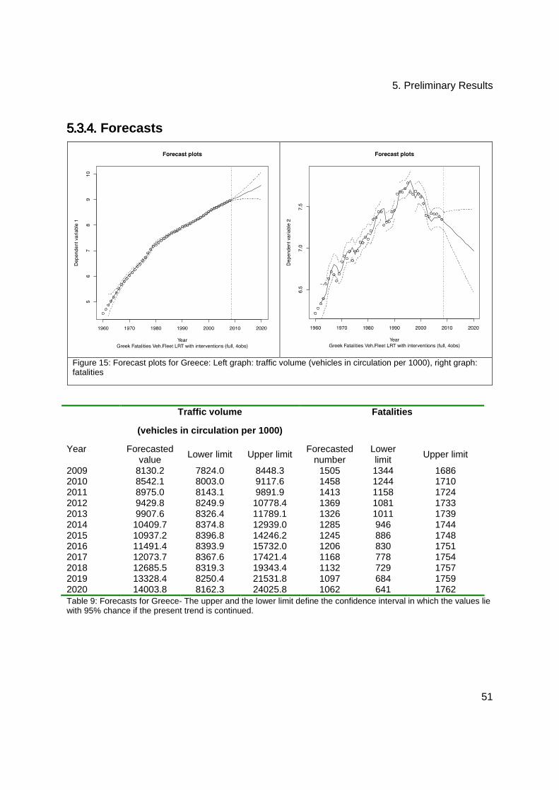
5. Preliminary Results
51
5.3.4.5.3.4.5.3.4.5.3.4. Forecasts
Figure 15: Forecast plots for Greece: Left graph: traffic volume (vehicles in circulation per 1000), right graph: fatalities
Traffic volume
(vehicles in circulation per 1000)
Fatalities
Year Forecasted value
Lower limit Upper limit Forecasted
number Lower limit
Upper limit
2009 8130.2 7824.0 8448.3 1505 1344 1686 2010 8542.1 8003.0 9117.6 1458 1244 1710 2011 8975.0 8143.1 9891.9 1413 1158 1724 2012 9429.8 8249.9 10778.4 1369 1081 1733 2013 9907.6 8326.4 11789.1 1326 1011 1739 2014 10409.7 8374.8 12939.0 1285 946 1744 2015 10937.2 8396.8 14246.2 1245 886 1748 2016 11491.4 8393.9 15732.0 1206 830 1751 2017 12073.7 8367.6 17421.4 1168 778 1754 2018 12685.5 8319.3 19343.4 1132 729 1757 2019 13328.4 8250.4 21531.8 1097 684 1759 2020 14003.8 8162.3 24025.8 1062 641 1762 Table 9: Forecasts for Greece- The upper and the lower limit define the confidence interval in which the values lie with 95% chance if the present trend is continued.

D4.2: Forecasting traffic fatalities in European countries
52
5.4. Italy
5.4.1.5.4.1.5.4.1.5.4.1. Data
Figure 16: Traffic volume (number of vehicles) for Italy, 1980 to 2008; total number of observations in the series: 29)
Figure 17: Fatalities for Italy. 1980-1998 7days;: 1999 – 2008 30 days; total number of observations in the series: 29)..
The existing data collection in Italy is based on forms and survey methods introduced by the Italian Institute of Statistic (ISTAT) in 1991. Official ISTAT data about injury crashes started in this year. Before 1991, ISTAT gathered data for all crash severity levels. Another important date for crash data collection is 1999, when ISTAT extended the time period used for the definition of a road crash fatality from 7 days to 30 days.
The vehicle fleet (number of vehicles) has been used as exposure indicator. No relevant changes in reporting methods occurred during the period of study.
The trend of fatalities is decreasing during the last decade. An increment in fatalities can be observed during year 1991 and 1999.
5.4.2.5.4.2.5.4.2.5.4.2. Breakpoints There have been a number of events and interventions in the considered period that could affect the number of fatalities. Not all of them were considered for the LRT model development, since for some of these interventions, no significant change in fatalities was observed (e.g., seatbelt obligation in 1988, penalty point system in 2003). Years of considered events/interventions are:
1986: Safety helmet obligation. It has been considered through a level intervention on the risk.

5. Preliminary Results
53
1991: Change in road crash data collection introduced by ISTAT. It has been included in the model as explanatory variable.
1992: New Highway Code was introduced in Italy. It’s possible to see a decrease in 1993 in the number of fatalities. It has been considered through a level intervention on the risk.
1999: Change in the way of recording fatalities (from killed 7 days to killed 30 days). It has been included in the model as explanatory variable.
5.4.3.5.4.3.5.4.3.5.4.3. Development of risk
Figure 18: Italy -- Exposure (number of vehicles) and risk (fatalities per vehicles)
The model run to generate the output presented here was an LRT model with stochastic (random) levels and slopes for exposure as well as fatality risk (see Model 2.3 in Table A16 and A17 for details). The trends (level + slope) for each variable are depicted in Figure 18.
The risk has been declining in the considered period. The increased number of fatalities highlighted in the fatalities plot in the beginning and at the end of 1990s is smoothed down in the fatality risk plot.

D4.2: Forecasting traffic fatalities in European countries
54
5.4.4.5.4.4.5.4.4.5.4.4. Forecasts
Figure 19: Forecastplots for Italy: Left graph:traffic volume (number vehicles), right graph: fatalities
Traffic volume (vehicles ) Fatalities Year Estimated
value Lower limit
Upper limit
Estimated number
Lower limit
Upper limit
2009 49137743 47649834 50672114 4518 4161 4905 2010 50401627 47932529 52997914 4289 3795 4848 2011 51698019 48096336 55569414 4072 3466 4786 2012 53027756 48141713 58409698 3866 3163 4727 2013 54391696 48075859 61537259 3671 2883 4674 2014 55790718 47906738 64972159 3485 2624 4629 2015 57225724 47641999 68737324 3309 2385 4591 2016 58697641 47288813 72858945 3142 2164 4561 2017 60207417 46853913 77366708 2983 1960 4538 2018 61756026 46343660 82294035 2832 1773 4523 Table 10: Forecasts for Italy - The upper and the lower limit define the confidence interval in which the values lie with 95% chance if the present trend is continued.

5. Preliminary Results
55
5.5. UK
5.5.1.5.5.1.5.5.1.5.5.1. Data
Time
UK
traffi
c
1985 1990 1995 2000 2005 2010
420
440
460
480
500
520
Time
UK
fat
1985 1990 1995 2000 2005 2010
2500
3000
3500
4000
4500
5000
5500
Figure 20: Traffic volume (vehicle kilometres) for the UK, 1991 to 2009; total number of observations in the series:19
Figure 21: Fatalities for the UK, 1983 to 2009; total number of observations in the series:27
The data used in the modelling are the annual numbers of fatalities and the annual vehicle kilometres (traffic volume) for Great Britain and Northern Ireland, added together to give UK.
The data all come from national databases. The details of road crashes and casualties, for example, come from the national STATS19 database. Since 1949, police throughout Great Britain have recorded details of road crashes that involve personal injury using a single reporting system that is reviewed and updated regularly. The information about road crash casualties for Northern Ireland comes from the database of T1 crash reports compiled by the Police Service of Northern Ireland. Very few, if any, fatal crashes do not become known to the police. The annual volume of car traffic is measured by the National Road Traffic Survey (NRTS). The road traffic estimates are calculated by combining data collected by some 180 Automatic Traffic Counters (ATCs) and manual counts at approximately ten thousand sites per annum. Estimates of annual traffic volume are only available from 1991 in Northern Ireland.
Initially models of fatalities were fitted to the UK data using data from 1991. However, better fitting models can be developed using a longer time series. 1983 was chosen as a start year.

D4.2: Forecasting traffic fatalities in European countries
56
This has the advantage of minimising any effects of the compulsory wearing of seatbelts law introduced at the start of 1983 and minimising the number of traffic data that would need to be imputed for Northern Ireland (8 years) in the modelling process.
5.5.2.5.5.2.5.5.2.5.5.2. Development of exposure and risk
Smoothed state plots
UK fatals and traffic latent risk modelYear
Leve
l exp
osur
e
1985 1990 1995 2000 2005 2010
5.9
6.0
6.1
6.2
Smoothed state plots
UK fatals and traffic latent risk modelYear
Leve
l ris
k
1985 1990 1995 2000 2005 2010
1.6
1.8
2.0
2.2
2.4
2.6
Figure 22: Exposure (based on Vehicle kms) for UK
Figure 23: risk (fatalities per 109 vehicle kms) for UK.
The model run to generate the output presented here was an LRT model with stochastic (random) levels and slopes for exposure as well as fatality risk (see Model 2.1 in Table A20 and A21 for details). The trends (level + slope) for each variable are depicted in Figure 22 and 23.
Figure 23 shows how the fatality risk per billion (109) vehicles KM has developed in the UK between 1983 and 2009. It can be seen that overall the UK fatality risk has been declining for many years. The effects of the two recessions (periods of economic decline) in the early 1990s and in 2007 appear to have influenced the gradient of the risk curve, with it declining more steeply during these periods.

5. Preliminary Results
57
5.5.3.5.5.3.5.5.3.5.5.3. Forecasts
Forecast plots
Year
Dep
ende
nt v
aria
ble
1
UK fatals and traffic latent risk model
1990 2000 2010 2020
5.9
6.0
6.1
6.2
6.3
6.4
6.5
Forecast plots
Year
Dep
ende
nt v
aria
ble
2
UK fatals and traffic latent risk model
1990 2000 2010 2020
56
78
Figure 24: Forecast of traffic volume for the UK Figure 25: Forecast of fatalities for the UK
Traffic volume (vehicle kms / million)
Fatalities
Year Estimated value
Lower limit Upper limit Estimated number
Lower limit Upper limit
2010 520 510 530 2,035 1,830 2,262 2011 516 497 535 1,773 1,458 2,156 2012 512 483 542 1,545 1,137 2,100 2013 508 468 551 1,346 871 2,080 2014 504 453 562 1,173 658 2,092 2015 501 436 574 1,022 491 2,131 2016 497 420 588 891 361 2,198 2017 493 403 603 776 263 2,293 2018 489 386 620 677 189 2,418 2019 486 369 639 590 135 2,575 2020 482 352 659 514 95 2,768 Table 11: Forecasts for the UK- The upper and the lower limit define the confidence interval in which the values lie with 95% chance if the present trend is continued.

D4.2: Forecasting traffic fatalities in European countries
58
6. CONCLUSIONS AND NEXT STEPS In this deliverable a time series model was presented that allows the simultaneous modelling and forecasting of road safety fatalities and of traffic volume. Preliminary results are given for five European countries, Belgium, Greece, Spain, Italy, and the United Kingdom (UK). For none of those countries8, forecasts from a statistical model existed earlier.
6.1. Strengths of the analysis method In some cases, one might think that the forecasts look pretty much the same as what you would get when you took a ruler and drew a line right through the measurements from the previous years. So, why is it so important to rely on a statistical model (and in particular on the LRT model adopted in WP4) to make forecasts? There are three main reasons: (1) the forecasts are better, (2) they come with a confidence interval, and (3) they take variations of the traffic volume into account. Below, we discuss each of these points in turn.
First, forecasts based on the statistical model are generally better, because the fatality numbers in the past do not form a straight line. If they did, you would know exactly how to draw your line through them. In fact, in that case the results from any statistical model would be exactly the same as if you use your ruler... However, when the past results do not form a straight line (and we saw that this is often the case), the exact position of the line is not so obvious to determine. Should you draw a line through the most recent years? Or maybe include earlier years? The models applied here “find” the optimal position of the ruler9.
Second, the confidence interval is so important, because we do not want to fool anyone. Nobody can see into the future, and you need to know how much trust you can have in the forecasts. The results will sometimes be disappointing, as the confidence intervals are often wider than we would like them to be – but at least you know what you have. Forecasts presented without confidence intervals are probably not more reliable than those presented here.
Finally, one of the main conclusions yielded by the results of the analyses presented here is that traffic volume is the most important determinant of the number of fatalities. As a consequence, a change in the exposure to the risk is the most likely explanation for the change in fatalities (for example, the 2008 recession was associated with a reduction of fatalities all over Europe, which is most likely to a good part due to the reduction of the traffic volume observed for that period). For policy makers, who want to evaluate the functioning of the traffic system, this is important information in itself. However, the fatality risk is the variable that should actually be used to measure the success of the road safety system in a
8 For Great Britain, sophisticated forecasts exist (Broughton & Knowles, 2010) however, for the UK (Great Britain + Northern Ireland) this is not the case.
9 This is the work of the Kalman filter, a routine that goes through the whole series, identifies which number of data points in the observed series allow to best predict the next ones (still in the observed series), and automatically adjusts the weight that is given to the different past observations for the production of the forecast.

6. Conclusions and next steps
59
country. The analyses presented here model both exposure and fatality risk. They allow disentangling past effects of exposure and of risk on fatalities and it takes the past development of exposure into account when determining the forecasts and the confidence intervals for the number of fatalities.
6.2. Main results for the 5 countries In Belgium, we saw that a drop in the number of fatalities occurred after 2001 that could not be explained by a reduction in the growth of exposure. So here we have a genuine drop in the risk for fatal crashes. The change of direction observed at that time was just about “significant”, meaning that the model was a little doubtful whether this should be assumed to be a structural change in the development of fatality risk, or a mere coincidence. The present forecasts are based on the assumption that a structural change took place.
In Spain, the number of fatalities has been mostly rising up to the 90s and mostly dropping afterwards. If considered jointly with the traffic volume, however, it becomes clear that the fatality risk has been almost continuously decreasing. Although the fatality numbers suggest a turning point around 1990, the strong peak observed there turns out to be the result from the combination of a decreasing growth in traffic volume and of a decreasing risk. There is only one exception to this general rule, namely the 1985 recession where the actual risk increased while the growth in traffic volume was slowed down.
The results for Greece generally reveal a similar development as in Spain. The raw fatalities show an impressive turning point in 1995, but the isolation of exposure and risk suggests a relative smooth development of these two variables. There seems to be an exception to this between 1986 and 1990, where the risk suddenly dropped and rose again a couple of years later. It must be noted however, that this could result from an artefact of the Greek exposure measure. In the absence of data concerning the actual traffic volume, the size of the vehicle fleet was used. In the economical recession in 1986 and after, this could however be an overestimation of the actual traffic volume, which was probably reduced at that time. Due to the overestimation of the traffic volume, the fatality risk is underestimated.
In Italy, the trend of the raw fatality numbers was generally decreasing, with the exception of two periods where fatality numbers increased. Both increases are probably due to a change in registration. When correcting for these two registration changes - and when considering fatality risk rather than the raw numbers - a smooth decrease can be observed for the whole period, with only somewhat of a stagnation around the millennium break and a more steep decrease since 2001.
In the UK, the number of people killed has varied fairly erratically, with periods of slow decline in 1983-1990 and 1996-2003 separated by a period of more rapid decline between 1991 and 1995 and 2007 to 2009. The fatality risk however, has been declining for many years. The effects of the two recessions (periods of economic decline) in the early 1990s and in 2007 appear to have influenced the gradient of the risk slope, which declined more steeply during these periods.

D4.2: Forecasting traffic fatalities in European countries
60
6.3. Next steps The results of the analyses presented here are very encouraging. This pilot run, performed on a small number of countries will allow a revision of the guidelines for the analyses spread among the partners (see Appendix B), as well as of the reporting format for each country's analysis. The changes to be expected will concern the lay-out (e.g., table formats) rather than the core method of analysis. One change foreseen already is the adaptation of the level of confidence for the forecasts. In the present results, the forecasts are presented with 95% confidence intervals. While this is the usual scientific level a smaller interval seems more interesting for political purposes (e.g. the 50% confidence interval). Additionally, a sensitivity analysis will be conducted in order to assess the effect of certain modelling decisions (e.g., about the inclusion of an intervention) on the forecasts.
The next step to be taken after the revision is to apply the same method of analysis to the rest of the European countries. Data will be available from CARE, IRTAD, Eurostat, UNECE and also from national sources. We should be able to run models similar to the ones presented here – either with vehicle kilometres or with vehicle fleet data as exposure – for almost all European countries. For a small minority (one to three), oil consumption will have to be used as exposure indicator.
The model framework presented here offers a large number of opportunities for extensions. The most important one foreseen within this Work Package is the separate modelling of different road-user types and/or different age groups. The composition of the driving population along these two factors and their combination is known to affect the fatality risk quite strongly. For example, given that motorcycles suffer an increased fatality risk - as compared to other road-users - their contribution to the total of vehicle kilometres driven in a country can influence the overall risk observed for that country (e.g., SafetyNet 2009a). Moreover, the developments observed for different road-user groups are not necessarily similar (Stipdonk et al., 2009). Different age groups are known to have very different risks (younger drivers, higher crash risk; older road users higher vulnerability; e.g., SafetyNet 2009b, SafetyNet 2009c), and in the light of an ageing population the exposure and the risk for different age groups develops differently. For these reasons, the next step will be to set up a methodology to model different road user or age groups in parallel and to test this methodology for a number of countries.
6.4. In a nutshell We have presented a framework of time series modelling that models the road safety fatalities together with their most important determinant, the risk exposure or mobility. The results for five countries, Belgium, Greece, Spain, Italy, and the United Kingdom, show the past development of the fatality risk (i.e. the number of fatalities per vehicle kilometre or per vehicle), and they forecast the fatalities and the mobility up to 2020.

D4.2: Forecasting traffic fatalities in European countries
61
REFERENCES: Australian Bureau of Statistics (2009). When it’s not “business-as-usual”: implications for ABS time series. Retrieved 18.11.2010 from http://www.abs.gov.au/AUSSTATS/[email protected]/Lookup/1350.0Feature+Article1Aug+2009
Bijleveld, F. (2008). Time series analysis in road safety research using state space methods. SWOV-Dissertatiereeks, Leischendam, Nederland.
Bijleveld F., Commandeur J., Gould P., Koopman S. J. (2008),. Model-based measurement of latent risk in time series with applications. Journal of the Royal Statistical Society, Series A, 2008.
Broughton, J. and Knowles, J. (2010) Providing the numerical context for British casualty reduction targets. Safety Science 48, 1134-1141.
Commandeur, J. & Koopman, S.J. (2007) An Introduction to State Space Time Series Analysis. Oxford University Press.
COST 329, (2004). Models for traffic and safety development and interventions. European Commission. Directorate general for Transport, Brussels, 2004.
Elvik, R. (2010). The stability of long-term trends in the number of traffic fatalities in a sample of highly motorized countries. Accident Analysis and Prevention, 42, 245-260.
Gorr, W.L. & McKay, S.A. (2004) Application of tracking signals to detect times series pattern changes. Retrieved 18.11.2010 from http://www.heinz.cmu.edu/research/134full.pdf.
Hakkert, A.S, Gitelman, V. and Vis, M.A. (Eds.) (2007) Road Safety Performance Indicators: Theory. Deliverable D3.6 of the EU FP6 project SafetyNet.
Hakim, S., Shefer, D., & Hakkert, S. (1991) A critical review of macro models for road accidents. Accident Analysis and Prevention, 23, 5, 379-400.
Harvey A C and Durbin J (1986). The effects of seat belt legislation on British road casualties:A case study in structural time series modelling. Journal of the Royal Statistical Society, Series A 149: pp187-227.
Harvey A., (1989). Forecasting, structural time series models and the Kalman filter. Cambridge University Press, Cambridge , 1989.
Doran, G. T.(1981). There's a S.M.A.R.T. way to write management's goals and objectives. Management Review, Nov 1981, 70, 11.
Hauer, E. (2010). On prediction in road safety. Safety Science 48, 1111-1122.
Koppits, E. & Cropper, M. (2008). Why have traffic fatalities declined in industrialised countries? Journal of Transport, Economics & Policy, 42, 129-145.
Lassarre S., Annual bivariate models of traffic fatality risk. Dacota technical notes, INRETS, Marne la vallée, 2010.

References
62
Oppe, S. (1989). Macroscopic models for traffic and traffic safety. Accident Analysis and Prevention 21, 225-232.
Oppe S. (1991) Development of traffic and traffic safety: global trends and incidental fluctuations. Accident Analysis and Prevention, 23(5):413-22.
SafetyNet (2009a) Powered Two Wheelers, retrieved at November 13, 2010 from http:// ec.europa.eu/transport/road_safety/specialist/knowledge/pdf/powered_two_wheelers.pdf
SafetyNet (2009b) Novice Drivers, retrieved at November 13, 2010 from http:// ec.europa.eu/transport/road_safety/specialist/knowledge/pdf/novice_drivers.pdf
SafetyNet (2009c) Older Drivers, retrieved at November 13, 2010 from http:// ec.europa.eu/transport/road_safety/specialist/knowledge/pdf/older_drivers.pdf
Stipdonk, H.L. (ed.) (2008). Time series applications on road safety developments in Europe. Deliverable D7.10 of the EU FP6 project SafetyNet.
Van den Bossche, F. & Wets, G. (2003) A structural road accident model for Belgium.
Vis, M. & Van Gent, A.L. eds. (2007) Road Safety Performance Indicators: Country Profiles. Deliverable D3.7b of the EU FP6 Project SafetyNet.
Wegman, F., Eksler, V., Hayes, S., Lynam, D., Mosrsink, P., Oppe, S. (2005). Sunflower+6: A comparative study of the development of road safety in the SUNflower+6 countries: Final report. Leidschendam: SWOV.
West M., Harrison P., Bayesian forecasting and dynamic models. Springer-Verlag, New-York, 1989.
Yannis, G., et al., (2005). , State of the art on risk and exposure data. Deliverable 2.1 of the EU FP6 project SafetyNet.

D4.2: Forecasting traffic fatalities in European countries
63
APPENDIX A: DETAILED RESULTS The detailed results of the analyses that form the basis for Chapter 5 are presented in this appendix (Appendix A). Appendix B presents the instructions that formed the basis for conducting the analyses.
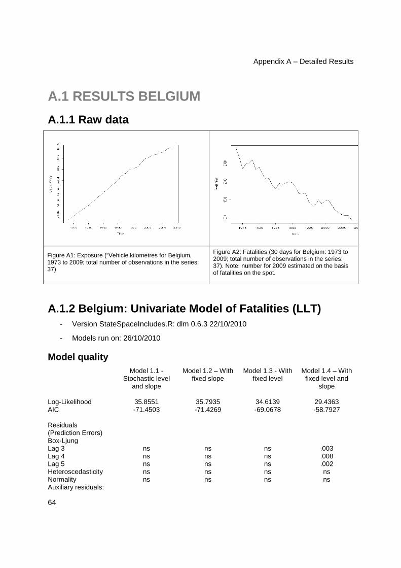
Appendix A – Detailed Results
64
A.1 RESULTS BELGIUM
A.1.1 Raw data
Figure A1: Exposure (“Vehicle kilometres for Belgium, 1973 to 2009; total number of observations in the series: 37)
Figure A2: Fatalities (30 days for Belgium: 1973 to 2009; total number of observations in the series: 37). Note: number for 2009 estimated on the basis of fatalities on the spot.
A.1.2 Belgium: Univariate Model of Fatalities (LLT) - Version StateSpaceIncludes.R: dlm 0.6.3 22/10/2010
- Models run on: 26/10/2010
Model quality Model 1.1 -
Stochastic level and slope
Model 1.2 – With fixed slope
Model 1.3 - With fixed level
Model 1.4 – With fixed level and
slope Log-Likelihood 35.8551 35.7935 34.6139 29.4363 AIC -71.4503 -71.4269 -69.0678 -58.7927 Residuals (Prediction Errors)
Box-Ljung Lag 3 ns ns ns .003 Lag 4 ns ns ns .008 Lag 5 ns ns ns .002 Heteroscedasticity ns ns ns ns Normality ns ns ns ns Auxiliary residuals:

D4.2: Forecasting traffic fatalities in European countries
65
Output : ns ns ns ns Level : ns ns ns ns Slope : ns ns ns ns Model prediction MPE4 0.33 -0.32 1.46 -1.35 MAPE4 0.49 0.51 1.46 1.35 MPE7 -2.62 -2.62 -2.63 -1.88 MAPE7 2.62 2.62 2.63 1.88 MPE10 -0.99 -1.21 -2.72 -0.25 MAPE10 1.52 1.70 2.98 1.01 Table A1 Diagnostic tests for local linear trend mo dels for Belgium
Model dynamics Model 1.1 -
Stochastic level and slope
Model 1.2 – With Fixed Slope
Model 1.3 - With Fixed level
Model 1.4 – With fixed level and slope
Observation errors 2εσ
2.1e-12 7.1e-07 - 0.0
4.3e-12 5.5e-07 - 0.0
0.0 2.9e-05 - 0.0
.005
.002 - .008
Level disturbances 2ξσ
3,0E-03 9,5E-04 - 6,1E-03
3,2E-03 1,3E-03 - 5,9E-03
/ /
Slope disturbances 2ζσ
3.2e-05 1.7e-07 - 0.0
/ 0.0 5.0e-05 - 0.0
/
Table A2 Model dynamics for local linear trend mode ls for Belgium
Figure A3: Smoothed state plots for Belgium Model 1.1: Left-hand graph: Trend; right-hand graph: Slope

Appendix A – Detailed Results
66
The Local Linear Trend Model for Belgium: Synthesis Table A1 indicates that the LLT model captures the development of the Belgian fatalities well. This is true for the LLT model with a stochastic level and slope, but also for the models where either the slope or the level are fixed. In both cases we see only a small decrease in the loglikelihood (or a small increase in the Akaike information criterion). This decrease is more important, however, when the level is fixed as compared to when the slope is fixed. This indicates that the dynamics of the Belgian road safety development are modelled somewhat more efficiently by a level that is allowed to vary than by a slope that is allowed to vary. However, when both state components are fixed there are clear problems: the likelihood statistics worsen (i.e. the likelihood decreases and the AIC increases) and residuals show clear signs of autoregression. The general trend in the Belgian fatalities is decreasing. However, the decrease is not a stable one. In 1985 to 1989, at the beginning of the series that is modelled here, the number of fatalities was increasing and the same is true between 1996 and 2001. As a consequence, the decrease in the periods in between is characterized by the model mostly as random variation in the level rather than as a structural decrease in the slope. The slope is slightly negative).
A.1.3 Belgium: Bivariate Model of Fatalities (LRT)
Belgian data and interventions The registration of traffic fatalities is based upon forms that are in use since 1991. Before there were other forms, which were not computerized however. The latest official number of victims killed in a crash on the spot or within 30 days after the crash concerns the year 2008. For 2009 an estimation is used, based on the number of fatalities on the spot.
The number of vehicle kilometres is estimated yearly on the basis of fuel consumption and traffic counts. The method presently employed has been introduced in 1995, which is where our series starts.
There have been a number of events and measures since 1985, for which it is possible that they had an effect on the number of fatalities. Subsequently we have given the most important measures that could have had an effect on the total number of fatalities.
FL1991 - In 1991 : regulations improved the position of vulnerable road users in traffic and seat-belts became mandatory in the back-seats. Moreover, the registration of crashes was changed in 1991 (the present queries were introduced, albeit on paper at that time). In 1991 we see a drop in the fatalities. In the model this is implemented by means of a level intervention on the fatality-risk.
FL1994 - In 1994 the legal threshold for blood-alcohol limit was lowered from 0.8 promille to 0.5 promille. This goes together with a drop in the fatalities. In the model this is implemented by means of a level intervention on the fatality-risk. This intervention was not significant, however. The model is therefore not reported.

D4.2: Forecasting traffic fatalities in European countries
67
FS2001 - 2001 is a year where many changes took place. First the registration was changed: crashes were registered on paper forms before 2001, while a computerized version of this form is used since then. This probably made a difference in terms of “lost forms”. Second, the whole Belgian police system was reformed at that time, and this may temporarily have given crash registration a lower priority. At the same time however, the statistical office paid more attention to the issue of missing crash forms for fatal victims (as registered by the hospitals). From 2002 on, these fatal victims for whom there was no crash form were included in the fatality counts. In 2001 a working group was founded by the IBSR with the aim of tracing the fatalities for which no crash form had been sent back to the police departments, resulting in a strong decrease in the number of non-registered fatal victims. Moreover, in 2001, the first Road Safety Action Plan (Etats Généraux de la Sécurité Routière) was launched, which was accompanied and followed by strong efforts in terms of enforcement, education, and road-engineering. For all these reasons, 2001 certainly qualifies for a breakpoint. A-priori, however, it is unclear whether we should expect improved registration to have lead to a higher number of fatal victims, or whether the increased of road safety efforts lead to a reduction in the number of fatal victims. The fatality trend indicates however that the latter occurred given the decrease (that continues well beyond 2001), and that even if fatalities numbers temporarily increased because of registration changes, the trend kept decreasing.
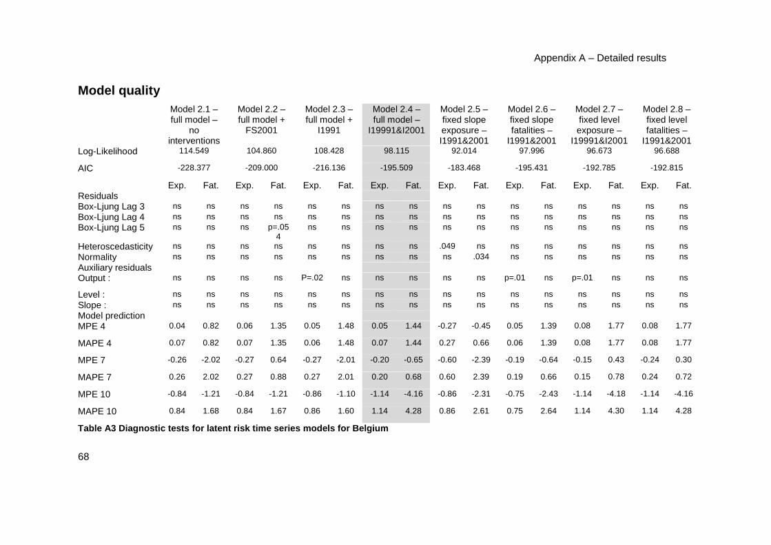
Appendix A – Detailed results
68
Model quality Model 2.1 –
full model – no
interventions
Model 2.2 – full model +
FS2001
Model 2.3 – full model +
I1991
Model 2.4 – full model –
I19991&I2001
Model 2.5 – fixed slope exposure – I1991&2001
Model 2.6 – fixed slope fatalities –
I1991&2001
Model 2.7 – fixed level exposure –
I19991&I2001
Model 2.8 – fixed level fatalities –
I1991&2001 Log-Likelihood 114.549 104.860 108.428 98.115 92.014 97.996 96.673 96.688
AIC -228.377 -209.000 -216.136 -195.509 -183.468 -195.431 -192.785 -192.815
Exp. Fat. Exp. Fat. Exp. Fat. Exp. Fat. Exp. Fat. Exp. Fat. Exp. Fat. Exp. Fat. Residuals Box-Ljung Lag 3 ns ns ns ns ns ns ns ns ns ns ns ns ns ns ns ns Box-Ljung Lag 4 ns ns ns ns ns ns ns ns ns ns ns ns ns ns ns ns Box-Ljung Lag 5 ns ns ns p=.05
4 ns ns ns ns ns ns ns ns ns ns ns ns
Heteroscedasticity ns ns ns ns ns ns ns ns .049 ns ns ns ns ns ns ns Normality ns ns ns ns ns ns ns ns ns .034 ns ns ns ns ns ns Auxiliary residuals Output : ns ns ns ns P=.02 ns ns ns ns ns p=.01 ns p=.01 ns ns ns
Level : ns ns ns ns ns ns ns ns ns ns ns ns ns ns ns ns Slope : ns ns ns ns ns ns ns ns ns ns ns ns ns ns ns ns Model prediction MPE 4 0.04 0.82 0.06 1.35 0.05 1.48 0.05 1.44 -0.27 -0.45 0.05 1.39 0.08 1.77 0.08 1.77
MAPE 4 0.07 0.82 0.07 1.35 0.06 1.48 0.07 1.44 0.27 0.66 0.06 1.39 0.08 1.77 0.08 1.77
MPE 7 -0.26 -2.02 -0.27 0.64 -0.27 -2.01 -0.20 -0.65 -0.60 -2.39 -0.19 -0.64 -0.15 0.43 -0.24 0.30
MAPE 7 0.26 2.02 0.27 0.88 0.27 2.01 0.20 0.68 0.60 2.39 0.19 0.66 0.15 0.78 0.24 0.72
MPE 10 -0.84 -1.21 -0.84 -1.21 -0.86 -1.10 -1.14 -4.16 -0.86 -2.31 -0.75 -2.43 -1.14 -4.18 -1.14 -4.16
MAPE 10 0.84 1.68 0.84 1.67 0.86 1.60 1.14 4.28 0.86 2.61 0.75 2.64 1.14 4.30 1.14 4.28
Table A3 Diagnostic tests for latent risk time seri es models for Belgium

D4.2: Forecasting traffic fatalities in European countries
69
Model dynamics Model 2.1 –
Full model Model 2.2 – Full model + I2001
Model 2.3 – Full model + I1991
Model 2.4 – full model – I19991&I2001
Model 2.5 – fixed slope exposure – I1991&2001
Model 2.6 – fixed slope fatalities – I1991&2001
Model 2.7 – fixed level exposure – I19991&I2001
Model 2.8 – fixed level fatalities – I1991&2001
Exposure Observation errors
2εσ
1.0E-09 *
1.9E-06 2.5E-04
1.3E-07*
1.0E-06 2.1E-04
1.2E-07*
1.5E-06 2.1E-04
4.7E-09*
9.4E-07 1.3E-04
3.1E-07*
5.0E-07 7.0E-05
5.1E-08*
1.2E-06 1.5E-04
2.7E-05*
8.0E-06 2.2E-04
2.6E-05*
4.7E-06 1.6E-04
Level disturbances 2ξσ
8.0E-05*
2.9E-05 1.9E-04
8.6E-05*
5.0E-05 9.6E-04
8.1E-05*
3.8E-05 4.1E-04
9.2E-05*
4.4E-05 2.8E-04
2.2E-04*
1.3E-04 5.4E-04
8.8E-05*
4.2E-05 2.9E-04
7.1E-06*
1.5E-07 4.0E-04
Slope disturbances 2ζσ
1.8E-05*
5.5E-06 1.7E-04
1.4E-05*
4.1E-06 1.4E-04
1.6E-05*
7.0E-06 6.2E-05
1.2E-05*
4.1E-06 1.5E-04
1.4E-05*
2.5E-06 3.3E-05
4.0E-05 *
9.7E-06 1.6E-04
3.7E-05 *
6.8E-06 1.7E-04
Fatality (risk)
Observation errors 2εσ
3.3E-12 *
6.8E-07 3.5E-03
1.8E-04 *
9.6E-07 3.4E-03
3.2E-04 *
8.8E-07 4.2E-03
9.7E-05*
7.9E-07 4.1E-03
2.1E-04 *
7.6E-07 2.7E-03
1.6E-04 *
1.5E-06 4.0E-03
8.4E-04 *
7.9E-05 2.6E-03
8.6E-04 *
8.3E-05 2.6E-03
Level disturbances 2ξσ
2.4E-03*
8.8E-04 4.8E-03
8.5E-04 *
1.4E-06 6.1E-03
1.9E-03 *
2.8E-04 4.7E-03
1.8E-03 *
3.7E-04 4.2E-03
1.6E-03 *
6.4E-05 5.6E-03
1.9E-03 *
4.1E-04 4.3E-03
1.1E-08*
6.4E-07 3.3E-03
Slope disturbances 2ζσ
3.0E-06 *
1.8E-08 1.1E-04
3.6E-04 *
1.4E-0 6 1.7E-03
2.6E-05 *
1.1E-07 1.7E-04
1.2E-05 *
5.5E-0 8 3.4E-04
2.9E-04 *
1.6E-05 8.5E-04
4.6E-04*
1.8E-05 1.4E-03
4.4E-04 *
1.9E-05 1.4E-03
Intervention1
(2001) tβ
-8.2E-02 *
-1.6E-01 -7.4E-03
-1.7E-01 *
-2.6E-01 -8.8E-02
-0.142988*
-2.3E-01 -5.5E-02
-5.1E-02
-1.2E-01 1.4E-02
-2.8E-02
-6.3E-02 6.8E-03
-6.0E-02
-1.2E-01 5.1E-03
-6.0E-02
-1.3E-01 5.5E-03
Intervention2
(1991) tβ
-4.4E-02*
-8.4E-02 -3.7E-03
-0.131364*
-2.2E-01 -4.2E-02
-0.1555 *
-2.4E-01 -6.9E-02
-0.129419*
-2.2E-01 -4.1E-02
-0.126787*
-2.2E-01 -3.6E-02
Table A4 Model dynamics for latent risk time series models
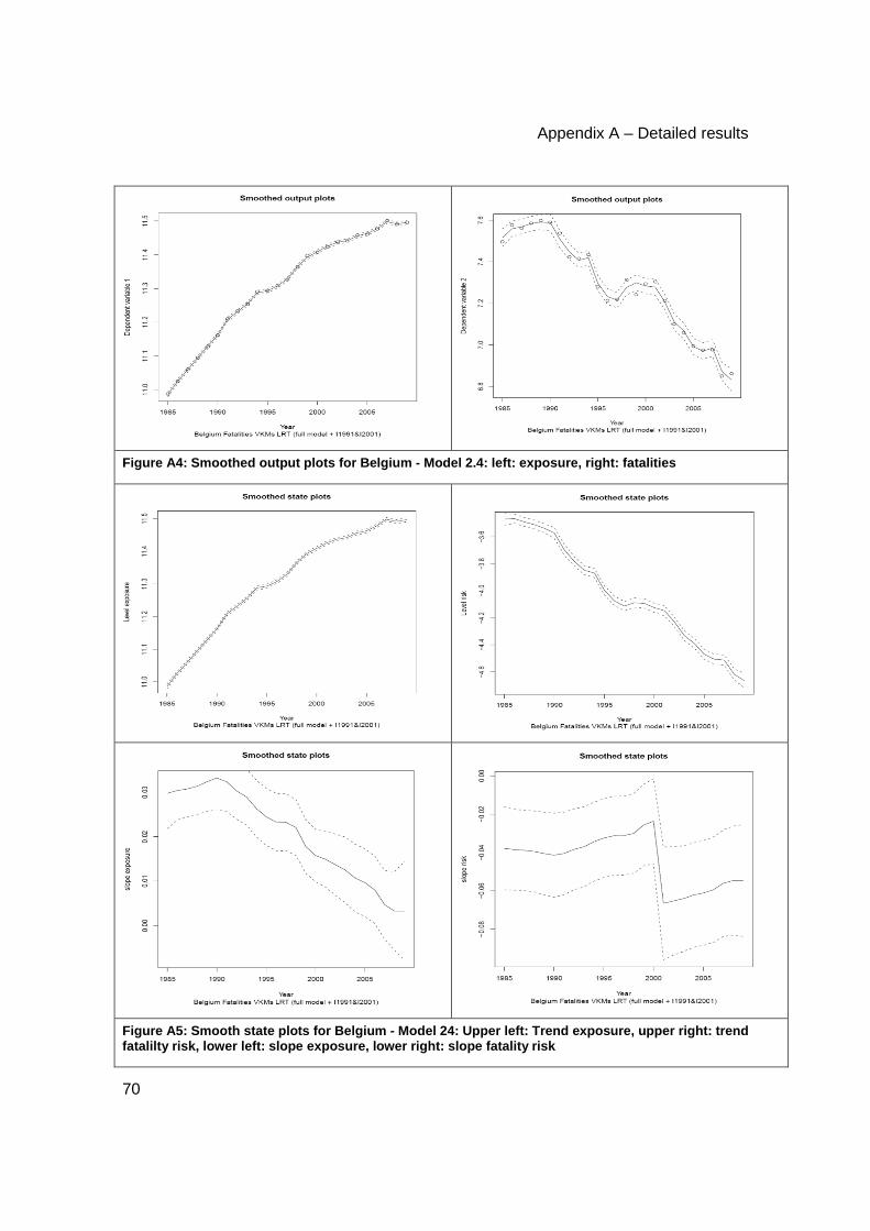
Appendix A – Detailed results
70
Figure A4: Smoothed output plots for Belgium - Model 2.4: left: exposure, right: fatalities
Figure A5: Smooth state plots for Belgium - Model 24 : Upper left: Trend exposure, upper right: trend fatalilty risk, lower left: slope exposure, lower r ight: slope fatality risk

D4.2: Forecasting traffic fatalities in European countries
71
Latent Risk Time Series Model for Belgium: Synthesi s In Table A3, an overview is given over the general characteristics of the models. The outcome of the residual tests are satisfactory. The very few significant results are all only just significant and this is to be expected when running such a large number of tests, each with a 5% chance to become significant without anything being wrong with the model. We therefore have no particular reason to doubt that the models capture the dynamics of the Belgian fatalities and exposure development well. Contrary to the local linear trend model, presented above, the latent risk time series model contains not only exposure as a second dependent variable, but also models the fatality risk (i.e. fatalities divided by traffic volume) rather than the fatalities themselves. This difference can be appreciated in the comparison of the output plots in Figure A4 and the state plots in Figure A5. For exposure the two trends look more or less the same. However, for the fatalities, Figure A4 shows the fatalities, while Figure A5 shows the fatality risk. We can see that for those periods where the number of fatalities actually increased (mid-80s and mid 90s) the fatality risk was stagnating but not increasing. This means that a stronger increase in traffic volume together with a stagnating risk was responsible for these two periods of increasing fatality numbers. In the comparisons between different models presented in Tables A3 and A4, it was first tested whether there were interventions that contributed significantly to the explanation of the past development. This was the case for the intervention on the fatality level in 1991 (Seat-belts in the back of the car became mandatory) and for the fatality slope in 2001. The slope intervention in 2001 is only just significant, which makes it difficult to decide whether it should be retained in the model. We have chosen to include it into the model with the following reasoning: the 2001 intervention on the slope indicates a change from stagnation in the risk before 2001 to a clear decrease in risk afterwards. This goes together with the start of the road safety action plan (Etats Généraux de la Sécurité Routière) which was launched then. The results of the intervention leave us in some doubt, whether the decrease following the road safety action plan was simply the result of random variation or whether a structural break did actually take place. For the forecasts, the assumption of a structural break leads to lower forecasts in the next years than the assumption that the post-2001 decrease was just due to random variation. Given that the forecasts will form the basis for target setting, we will assume the more ambitious model, which assumes that a structural change took place after launching the road safety action plan. Based on the model with two interventions (level 1991, slope 2001) it was further tested whether stochastic components (level and slope for exposure; level and slope for risk) could be fixed. In all cases, fixing a component lead to a model with a lower likelihood and a higher AIC (although when fixing the slope for the fatality risk the fit of the model decreased only slightly).

Appendix A – Detailed results
72
The Latent Risk Time Series Model for Belgium: Fore casts
Figure A6: Forecastplots for Belgium Model 2.4: Upper graph: exposure, lower graph: fatalities
Final model Belgium– Latent Risk Model 2.4 with Interventions at 1991 (level fatalities) and 2001 (slope fatalities) – Forecasts
Exposure (vehicle kms / million) Fatalities
Year Estimated value
Lower limit
Upper limit
Estimated number
Lower limit
Upper limit
2010 98666 96410 100975 880 779 995 2011 98990 95450 102661 836 705 992 2012 99315 94473 104405 794 642 983 2013 99641 93430 106265 755 586 971 2014 99968 92311 108259 717 536 958 2015 100296 91119 110397 681 491 944 2016 100625 89857 112684 647 450 930 2017 100956 88532 115123 614 412 915 2018 101287 87149 117719 584 378 901 2019 101620 85714 120477 554 347 886 2020 101953 84233 123401 527 318 871 Note: The upper and the lower limit define the confidence interval in which the values lie with 95% chance if the present trend is continued.

D4.2: Forecasting traffic fatalities in European countries
73
A.2 RESULTS SPAIN
A.2.1 Raw data
Figure A7: Traffic volume (vehicle kilometres) for Spain 1961 to 2008; total number of observations in the series: 48)
Figure A8: Fatalities (24h for Spain 1961 to 2008; total number of observations in the series: 48)
A.2.2 Spain: Univariate Model of Fatalities (LLT) - Version StateSpaceIncludes.R: dlm 0.6.3 22/10/2010
- Models run on: 17/11/2010
Model quality
Model 1.1 - Full
Model - Stochastic level and slope
Model 1.2 – With fixed
slope
Model 1.3 - With Fixed
level
Model 1.4 - Slope and level fixed
Log-Likelihood 91.6315 77.7357 91.6315 13.1233
AIC -183.14 -155.39 -183.181 -26.2059
Residuals

Appendix A – Detailed results
74
(Prediction Errors)
Box-Ljung
Lag 3 ns <0.001 ns <0.001
Lag 4 0.02 <0.001 0.02 <0.001
Lag 5 0.04 0.001 0.04 <0.001
Heteroscedasticity ns 0.06 ns <0.001
Normality ns ns ns 0.03
Auxiliary residuals:
Output : ns ns ns 0.01
Level : ns ns ns 0.06
Slope : ns <0.001 ns <0.001
Model prediction
++ MPE -1.025 -4.488 -1.025 -9.329
++ MAPE 1.025 4.488 1.025 9.329
Table A5. Diagnostic tests for Spain - Local Linear Trend Models ++ Model prediction Errors have been calculated inc luding in the model 5 forecastobs.
Figure A9 Standardised Residuals for Spain Model 1. 1 (Full model)

D4.2: Forecasting traffic fatalities in European countries
75
Model dynamics
Model 1.1 - Stochastic
level and slope Model 1.2 - Fixed Slope Model 1.3 - Fixed level
Model 1.4 - Fixed slope and level
Observation errors
2εσ
6.20 e-04 (2.69 e-04 - 1.13 e-03)
3.19 e-11 (1.09 e-07 - 6.55 e-04)
6.21 e-04 (2.70 e-04- 1.15 e-03)
8.85 e-02 (5.61 e-02 - 1.29 e-01)
Level disturbances
2ξσ
4.20 e-13 (1.25 e-13 - 7.79 e-03)
6.89 e-03 (4.41 e-03 - 9.94 e-03)
/ 0
Slope disturbances
2ζσ
1.62 e-03 (7.26 e-04 - 3.07 e-03)
/ 1.62 e-03
(7.03 e-04 - 2.84 e-03) 0
Table A6. Model dynamics for Spain - Local Linear T rend Models
Figure A10: Smoothed state plots for Spain -- Model 1.1: Left-hand graph: Level; right-hand graph: Slope
The Local Linear Trend Model: Synthesis Table A5 indicates that the Local Linear Trend (LLT) model captures the development of the Spanish fatalities quite well. The model residuals are approximately homoscedastic and normally distributed but are not independent, as can be seen with the Box-Ljung Tests. This could suggest that residuals might be auto-correlated. This is true for both, the LLT model with a stochastic level and slope (full model), and for the model where the level is fixed (fixed level model), but not for the model where the slope is fixed. For the latter, the residuals are heteroscedastic. The LLT fixed level model shows the same log-likelihood than the full model and a small decrease in the Akaike Information criterion (AIC). While for the LLT slope fixed model there is an important decrease in the log-likelihood and an increase in the AIC. This

Appendix A – Detailed results
76
indicates that the dynamics of the Spanish fatalities is more efficiently modelled by a slope that is allowed to vary than by a level that is allowed to vary. When both level and slope are fixed the log-likelihood statistic as well as the Akaike Information criterion worsen, and the residuals show sings of autocorrelation.
There is not a general pattern, but a high variability in the annual number of Spanish fatalities between 1961 and 2008. As can be seen at the smoothed state plots there are periods where the slope decreases, other where it is stable and other where it increases (Figure A10). The periods with greater reduction in the number of fatalities are 1990-1995 and from 2003.
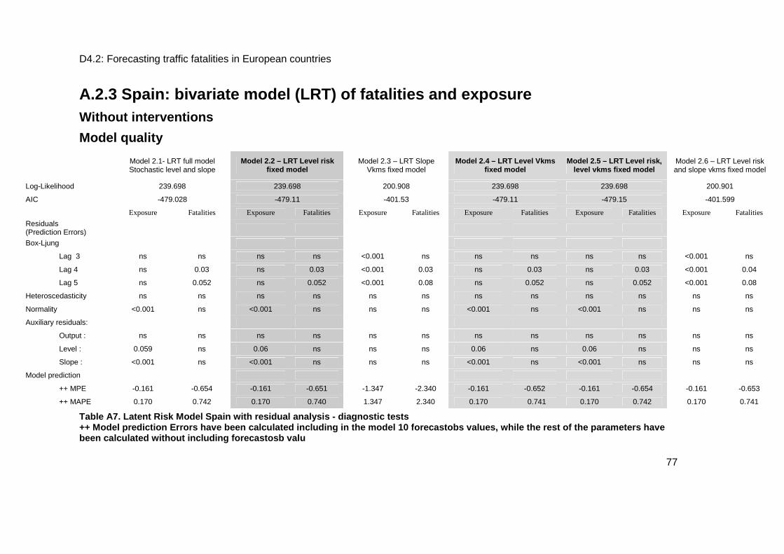
D4.2: Forecasting traffic fatalities in European countries
77
A.2.3 Spain: bivariate model (LRT) of fatalities an d exposure Without interventions
Model quality
Model 2.1- LRT full model Stochastic level and slope
Model 2.2 – LRT Level risk fixed model
Model 2.3 – LRT Slope Vkms fixed model
Model 2.4 – LRT Level Vkms fixed model
Model 2.5 – LRT Level risk, level vkms fixed model
Model 2.6 – LRT Level risk and slope vkms fixed model
Log-Likelihood 239.698 239.698 200.908 239.698 239.698 200.901
AIC -479.028 -479.11 -401.53 -479.11 -479.15 -401.599
Exposure Fatalities Exposure Fatalities Exposure Fatalities Exposure Fatalities Exposure Fatalities Exposure Fatalities
Residuals (Prediction Errors)
Box-Ljung
Lag 3 ns ns ns ns <0.001 ns ns ns ns ns <0.001 ns
Lag 4 ns 0.03 ns 0.03 <0.001 0.03 ns 0.03 ns 0.03 <0.001 0.04
Lag 5 ns 0.052 ns 0.052 <0.001 0.08 ns 0.052 ns 0.052 <0.001 0.08
Heteroscedasticity ns ns ns ns ns ns ns ns ns ns ns ns
Normality <0.001 ns <0.001 ns ns ns <0.001 ns <0.001 ns ns ns
Auxiliary residuals:
Output : ns ns ns ns ns ns ns ns ns ns ns ns
Level : 0.059 ns 0.06 ns ns ns 0.06 ns 0.06 ns ns ns
Slope : <0.001 ns <0.001 ns ns ns <0.001 ns <0.001 ns ns ns
Model prediction
++ MPE -0.161 -0.654 -0.161 -0.651 -1.347 -2.340 -0.161 -0.652 -0.161 -0.654 -0.161 -0.653
++ MAPE 0.170 0.742 0.170 0.740 1.347 2.340 0.170 0.741 0.170 0.742 0.170 0.741
Table A7. Latent Risk Model Spain with residual ana lysis - diagnostic tests ++ Model prediction Errors have been calculated inc luding in the model 10 forecastobs values, while th e rest of the parameters have been calculated without including forecastosb valu

Appendix A – Detailed results
78
Figure A11: Standardised Residuals for Spain - Mode l 2.1: Left-hand graph: residuals VKMs; right-hand graph: residuals fatalities
Figure A12: State auxiliary residual test for Spain Model 2.1: Left-hand graph: Level exposure; right-hand graph: Slope exposure

D4.2: Forecasting traffic fatalities in European countries
79
Models with interventions
Spanish data and interventions The registration of the Spanish traffic fatalities is based upon forms fulfilled by the police. There have been changes in the way of registration along the period of study, but we believe that it did not influenced the reporting number of fatalities. In 1993 it was adopted the new definition of fatalities at 30 days, but in the series studied we only included fatalities at 24h for all the period 1961-2009.
The number of vehicle-kms is estimated and includes only non-urban trips. The quality of estimates is unknown. From 1994 there is a change in the way of calculation, but it seems that it does not cause any break in the series.
As there are no breaks for the fatalities and vehicle-kms series related to reporting, no explanatory variables have been included in the models to adjust for .
There have been a number of events and measures since 1961, that could have affected the number of fatalities and the exposure. We describe those which have been found significant in the models:
1973: In 1973 there was an oil crisis that began on October 17, which resulted in a price increase of oil. The price increase coupled with the heavy reliance that had the industrialized world on OPEC oil, triggered a strong inflationary effect and reduced economic activity in the affected countries.
Regarding road safety interventions in 1973 the limit of alcohol was established in 0,8g/l and in 1974 the first speed limit was established for highways (130km/h). In Spain we can see a decrease in 1973 in the number of fatalities and in the number of veh-kms. In the model this is considered by means of a level and slope interventions on the exposure in 1973.
Interventions in the model: VL1973, VS1973
1984: In the mid eighties there is a period of economical expansion. The number of fatalities show a great increase. It is included in the model as an intervention as exposure slope.
Interventions in the model: VS1984
1989: After a long period of economical expansion, at the end of the eighties and early nineties there is a period of economic recession. Regarding road safety interventions in 1989 the amount of fines were increased. 1989 is the year with the maximum number of fatalities along the period, from which there is an inflection and a change in the slope which starts to decrease. It is included in the model as an interventions as level and slope fatality risk.
Interventions in the model: FL1989, FS1989
1994: The economical recession started to recover in the middle nineties. In 1992 new road safety measures were implemented. These included the enforcement of helmet for two wheel motor users and seat-belt for the front car seats. Vehicle safety started to be more frequent in the Spanish vehicle fleet. The number of fatalities from 1994 changes the previous

Appendix A – Detailed results
80
decreasing slope and becomes stable until 2003. It is included in the model as an intervention as fatality risk slope.
Interventions in the model: FS1994
2007: From 2007 the number of vehicles-km decreased, probably due to the beginning of the worldwide economical crisis. This can be seen clearly in 2008. It is included in the model as interventions for level and slope exposure. Regarding road safety measures in June 2006 the Penalty Points System was implemented and in December there was a Reform of the Penal Code which increased the severity of the infractions including prison. The number of fatalities decrease sharply.
Interventions in the model: VL2007, VS2007
Significant interventions:
- VS1973: 1973 slope exposure (Vkms)
- VS1984: 1984 slope exposure (Vkms)
- FS1989: 1989 slope risk
- FS1994: 1994 slope risk
- VL2007: 2007 level risk

D4.2: Forecasting traffic fatalities in European countries
81
Model quality Selected model Spain: Model 3.4 LRT level risk and level vkms fixed model with Interventions at 1973 (slope exposure), 1984 (slope exposure), 1989 (slope risk), 1994 (slope ri sk) and 2007 (level exposure).
Table A8. Diagnostic tests for Spain - latent risk time series models with interventions
Model 3.1 – LRT FULL MODEL (All stochastic components) All significant interventions
Model 3.2 – LRT LEVEL RISK FIXED MODEL
All significant interventions
Model 3.3 – LRT LEVEL VKMS FIXED
All significant interventions
Model 3.4 – LRT LEVEL RISK AND LEVEL VKMS FIXED All significant interventions
Log-Likelihood 218.321 218.921 218.92 218.92
AIC -437.474 -437.555 -437.555 -437.596
Exposure Fatalities Exposure Fatalities Exposure Fatalities Exposure Fatalities
Residuals (Prediction Errors)
Box-Ljung
Lag 3 ns ns ns ns ns ns ns ns
Lag 4 ns 0.03 ns 0.03 ns 0.03 ns 0.03
Lag 5 ns 0.04 ns 0.04 ns 0.04 ns 0.04
Heteroscedasticity ns ns ns ns ns ns ns ns
Normality ns ns ns ns ns ns ns ns
Auxiliary residuals :
Output : ns ns ns ns ns ns ns ns
Level : ns ns ns ns ns ns ns ns
Slope : ns ns ns ns ns ns ns ns
Model prediction
MPE4 -0.1039 -0.4668 -0.104 -0.466 -0.103768 -0.467588 -0.1038 -0.4661
MAPE4 0.1528 0.7972 0.153 0.797 0.152765 0.797396 0.1528 0.7969
MPE7 -0.7282 -2.9187 -0.728 -2.918 -0.728306 -2.9152 -0.7283 -2.9213
MAPE7 0.7282 2.9918 0.728 2.992 0.728306 2.98865 0.7283 2.9941
MPE10 -1.1735 -5.5687 -1.173 -5.571 -1.17316 -5.56406 -1.1724 -5.5731
MAPE10 1.1735 5.5687 1.173 5.571 1.17316 5.56406 1.1724 5.5731

Appendix A – Detailed results
82
Figure A13: Standardised Residuals for residual-ana lysis FATALITIES: Spain - Model 3.1. LRT full model with the signific ant interventions

D4.2: Forecasting traffic fatalities in European countries
83
Model dynamics
Table A9. Model dynamics for Spain - latent risk ti me series models with interventions – Hyperparamete rs and parameters*p<0.05
Selected model Spain: Model 3.4 LRT level risk and level vkms fixed model with Interventions at 1973 (slope exposure), 1984 (slope exposure), 1989 (slope risk), 1994 (slope ri sk) and 2007 (level exposure).
Model 3.1 – LRT FULL MODEL (All stochastic components) All significant interventions
Model 3.2 – LRT LEVEL RISK FIXED MODEL
All significant interventions
Model 3.3 – LRT LEVEL VKMS FIXED
All significant interventions
Model 3.4 – LRT LEVEL RISK AND LEVEL VKMS FIXED
All significant interventions
Exposure
Observation errors 2εσ 1.58 e-05
(5.78 e-06 – 5.88 e-05) 1.58 e-05
(5.28 e-06 – 5.60 e-05) 1.59 e-05
(5.30 e-06 – 5.92 e-05) 1.59789e-05
(5.24 e-06 – 5.53 e-05)
Level disturbances 2ξσ 1.79 e-12
(1.98 e-06 – 3.10 e-04) 1.88 e-10
(4.01 e-08 – 8.59 e-05) 0 0
Slope disturbances 2ζσ 1.05 e-04
(6.91 e-05 – 1.79 e-04) 1.05 e-04
(5.99 e-05 – 1.79 e-04) 1.05 e-04
(6.07 e-05 – 1.72 e-04) 1.05 e-04
(5.99 e-05 – 1.81 e-04) ( Interventions )
tβ
VL2007 VS1973 VS1984
0.0368054 -0.0880679 0.0361093
0.0368002 -0.0880894 0.0360709
0.0368068 -0.0880949 0.0360657
0.0368154 -0.0881083 0.0360603
Fatality (risk)
Observation errors 2εσ 3.01 e-04
(8.22 e-05 – 6.54 e-03) 3.01 e-04
(8.44 e-05 – 6.49 e-04) 3.01 e-04
(9.60 e-05 – 6.5 e-04) 2.99 e-04
(7.65 e-05 – 6.68 e-04)
Level disturbances 2ξσ 3.79 e-10
(8.14 e-07 - 7.41 e-03) 0
3.37 e-10 (2.82 e-07 – 2.29 e-03)
0
Slope disturbances 2ζσ 7.42 e-04
(1.83 e-04 – 8.63 e-04) 4.72 e-04
(1.99 e-04 – 8.41 e-04) 4.72 e-04
(1.79 e-04 – 8.8 e-04) 4.69 e-04
(1.86 e-04 – 8.8 e-04) ( Interventions )
tβ
FS1989 FS1994
-0.136944 0.131192
-0.136957 0.131185
-0.136965 0.13117
-0.136988 0.131126
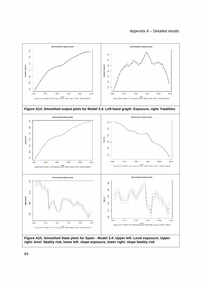
Appendix A – Detailed results
84
Figure A14. Smoothed output plots for Model 3.4: Le ft-hand graph: Exposure, right: Fatalities
Figure A15. Smoothed State plots for Spain - Model 3.4: Upper left: Level exposure; Upper right: level fatality risk, lower left: slope expo sure, lower right: slope fatality risk
D4.2: Forecasting traffic fatalities in European countries
85
The Latent Risk Time series Model for Spain: Synthe sis As it was said above, the Local Linear Trend (LLT) model (Table A5) that best captures the development of the Spanish fatalities is the LLT model with fixed level and stochastic slope. Regarding to the LLT model, the Latent Risk Time series (LRT) models includes not only exposure as a second dependent variable, but also models the fatality risk (i.e. fatalities divided by traffic volume) rather than the fatalities themselves. Therefore, based on the LRT model with a fixed level risk, it was further tested whether the stochastic components for the exposure (level and slope exposure) could be fixed. These results are presented in Table A5, and show that fixing only the level risk component, or fixing the level risk and the level exposure components, lead two models with a high log-likelihood, almost equal to the full model (all stochastic components) and a low AIC, lower than the full model.
From the interpretation of the “state auxiliary residuals” plot of each of the components of the LRT level risk fixed model we decided the candidate interventions to include in the model, that are explained in section 1.3.1. They were tested each one separately and then all together from those which were significant. Table A8 presents the comparison between the LRT full model with the significant interventions (VS1973, VS1984, FS1989, FS1994 and VL2007) (model 3.1), the LRT level risk fixed model (model 3.2), the LRT level exposure (vkms) fixed model (model 3.3) and the LRT level risk and level exposure (vkms) fixed model (model 3.4). Tables A8 and A9 show the models quality and dynamics results of the four models.
Table A8 shows that the three models have the same positive results, similar log-likelihood that the full model with the same interventions and lower AIC. All tests of the residuals are not significant in the case of exposure and, in the case of fatalities, there are only significant values for lags 4 and 5 of the Box-Ljung Test. But the last model (model 3.4) lead an AIC a little smaller than the others models. Therefore the final model is the LRT level risk and level exposure (vkms) fixed with the following significant interventions: slope exposure intervention in 1973 (VS1973) and in 1984 (VS1984), slope risk intervention in 1989 (FS1989), slope risk intervention in 1994 (FS1994) and level exposure intervention in 2007 (VL2007). The outputs plots for the final model are showed in Figure A14 and the state plots in Figure A15. For exposure the two trends look more or less the same (smoothed output plot for dependent variable 1 and smoothed state plots level exposure). However, for the fatalities and risk are different. Figure A14 (smoothed output plot for dependent variable 2) shows the fatalities trend, while Figure A15 (smoothed state plots level risk) shows the fatality risk trend.
For the initial period where the number of fatalities increased (1961-1982) the fatality risk was decreasing. This means that a stronger increase in traffic volume was responsible for this increasing fatality numbers. As the traffic volume has exceeded the number of fatalities in terms of risk there has been a reduction over the period. In the middle of this period there is a stagnation in the decrease in risk because the oil crisis of 1973 has reduced the traffic volume but the number of fatalities continues to rise. In contrast, the sharp increase in the number of fatalities in the 1985-1989 period itself has resulted in an increased risk in this period, because the increase in traffic volume has been proportionately smaller than the number of deaths. This period coincides with the

Appendix A – Detailed results
86
country's economic expansion from 1984. Another remarkable period is the 1990-1994, where there was a sharp decrease in the number of fatalities even though the traffic volume continued to rise despite the onset of the crisis of 90’s, and therefore there is a strong risk reduction. Another period to stress in our series is the 1994-2003 which coincides with the beginning of a new situation of economical expansion which stabilizes the number of deaths even though the traffic volume continues to rise, representing a risk reduction. Finally, the last period 2004-2007, where road safety is incorporated into the political agenda as a priority, there has been sharp decrease in the number of deaths and a slowdown in the traffic volume resulting in a marked risk reduction. It is noteworthy, however, that the intervention of around 2003 has not been significant in the final model.
The Latent Risk Time Series Model: Forecasts
Figure A16. Forecastplost for Model 3.4. Left graph : Exposure, Right graph: Fatalities
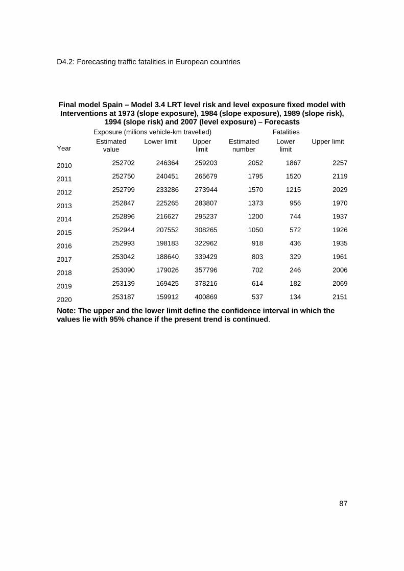
D4.2: Forecasting traffic fatalities in European countries
87
Final model Spain – Model 3.4 LRT level risk and level exposure fixed m odel with Interventions at 1973 (slope exposure), 1984 (slope exposure), 1989 (slope risk),
1994 (slope risk) and 2007 (level exposure) – Forecasts Exposure (milions vehicle-km travelled) Fatalities
Year Estimated
value Lower limit Upper
limit Estimated number
Lower limit
Upper limit
2010 252702 246364 259203 2052 1867 2257
2011 252750 240451 265679 1795 1520 2119
2012 252799 233286 273944 1570 1215 2029
2013 252847 225265 283807 1373 956 1970
2014 252896 216627 295237 1200 744 1937
2015 252944 207552 308265 1050 572 1926
2016 252993 198183 322962 918 436 1935
2017 253042 188640 339429 803 329 1961
2018 253090 179026 357796 702 246 2006
2019 253139 169425 378216 614 182 2069
2020 253187 159912 400869 537 134 2151
Note: The upper and the lower limit define the conf idence interval in which the values lie with 95% chance if the present trend is continued .

Appendix A – Detailed results
88
A.3 RESULTS GREECE
A.3.1 Raw data
Figure A17: Exposure (Number of Vehicles in circulation for Greece from 1960 to 2008; total number of observations in the series: 49)
Figure A18: Fatalities (30 days, for Greece from 1960 to 2008; total number of observations in the series: 49)
A.3.2 Greece: Univariate Model of Fatalities (LLT) DaCoTAStateSpaceIncludes version: dlm 0.6.3 22/10/2010
Model initial date: Wed Nov 3 21:34:11 2010
Model quality In order to assess the model quality, the candidate models are run while holding a number of observations for validation. However, as can be seen from Figure A18, the nature of the data (i.e. the breakpoint in the mid 1990s) implies that the subsequent downwards trend is only supported by few data points. Therefore, as the number of observations that are left aside for validation (and therefore not for model estimation) increases, then the model is less likely to capture the current (and forecast) trend.
Having said that, three scenarios have been run, according to the specifications, i.e. keeping 4, 7 and 10 observations for validation, respectively.
Model 1.1 - Stochastic
level and slope

D4.2: Forecasting traffic fatalities in European countries
89
Log-Likelihood 81.71
AIC -163.29
Residuals (Prediction Errors)
Box-Ljung
Lag 3 n.s.
Lag 4 n.s.
Lag 5 p=0.048
Heteroscedasticity n.s.
Normality n.s.
Auxiliary residuals:
Output : n.s.
Level : n.s.
Slope : n.s.
MPE 4 0.229
MAPE 4 0.229
MPE7 -2.218
MAPE7 2.218
MPE10 -5.956
MAPE10 5.956
Table A10. Diagnostic tests for Greek local linear trend models (fatalities)

Appendix A – Detailed results
90
Figure A19: State (level) auxiliary residuals for Greece - Model 1.3 (forecastobs=4)
Figure A20: Standardized Residuals for Greece - Model 1.3 (forecastobs =4)
Model dynamics
Model 1.1 - Stochastic level and slope
Model 1.2 – With Fixed
Slope
Model 1.3 – With Fixed level
Observation errors 2εσ 3.82E-12 1.24E-11 0.00094
1.07e-06 - .0019 2.81e-07 -
0.0013 9.9e-05-0.0029
Level disturbances 2εσ 0.0039 0.0052 /
0.0021 - 0.0063 0.003 - 0.0078
Slope disturbances 2ζσ 8.37e-07 / 0.0016
8.4e-07 - 0.0004 0.0003 - 0.0042
Table A11: Local Linear Trend Model Greece - Hyperp arameters and parameters

D4.2: Forecasting traffic fatalities in European countries
91
Figure A21: Smoothed state plots for Greece - Model 1.1: Left-hand graph: Trend; right-hand graph: Slope
The Local Linear Trend Model for Greece: Synthesis The analysis presented in this section indicates that the LLT model may provide a reasonable modeling of the evolution of road crash fatalities in Greece. This is true both for the model in which both the slope and the level are allowed to vary, and in the model that assumes a fixed slope. However, some issues arise when the level is fixed. As discussed above, the trend of road crash fatalities in Greece is not monotonic in the period of analysis. An inspection of the right subfigures of Figure A21 indicates that the downward trend in the slope has increased after the late 1980s.
A.3.3 Greece: The bivariate model (LRT) of fataliti es and exposure
Interventions in Greece There are three main events that can be entered as interventions in the model for the period and data that are being analyzed:
I1986: in 1986 Greece encountered a financial crisis, which affected mobility and therefore exposure (note that –due to lack of the data- the exposure variable in the Greek dataset is vehicles in circulation and not direct exposure)
I1991: in 1991 Greece introduced an “old-car-exchange” scheme, under which old cars could be exchanged for a cash incentive to buy a new (safer and cleaner) car. While
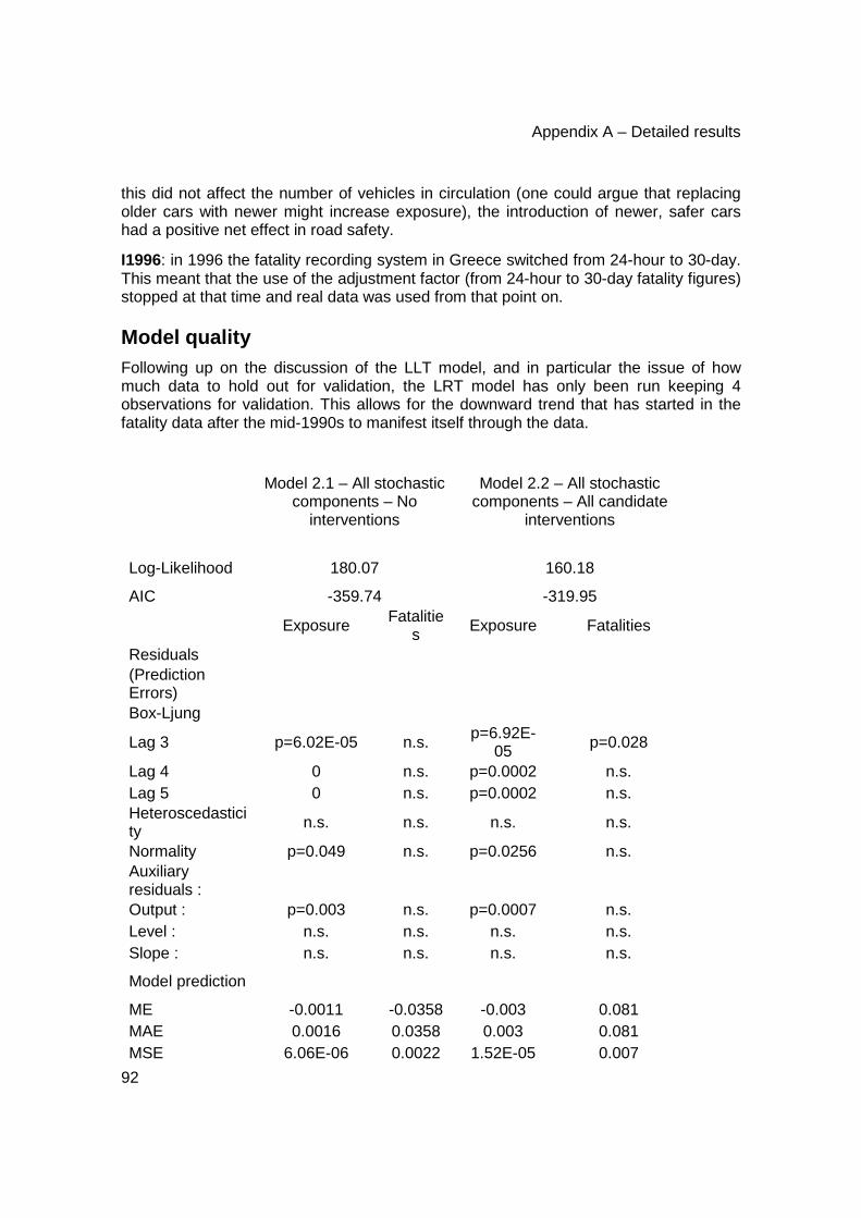
Appendix A – Detailed results
92
this did not affect the number of vehicles in circulation (one could argue that replacing older cars with newer might increase exposure), the introduction of newer, safer cars had a positive net effect in road safety.
I1996: in 1996 the fatality recording system in Greece switched from 24-hour to 30-day. This meant that the use of the adjustment factor (from 24-hour to 30-day fatality figures) stopped at that time and real data was used from that point on.
Model quality Following up on the discussion of the LLT model, and in particular the issue of how much data to hold out for validation, the LRT model has only been run keeping 4 observations for validation. This allows for the downward trend that has started in the fatality data after the mid-1990s to manifest itself through the data.
Model 2.1 – All stochastic
components – No interventions
Model 2.2 – All stochastic components – All candidate
interventions
Log-Likelihood 180.07 160.18
AIC -359.74 -319.95
Exposure Fatalities Exposure Fatalities
Residuals (Prediction Errors)
Box-Ljung
Lag 3 p=6.02E-05 n.s. p=6.92E-05 p=0.028
Lag 4 0 n.s. p=0.0002 n.s. Lag 5 0 n.s. p=0.0002 n.s. Heteroscedasticity n.s. n.s. n.s. n.s.
Normality p=0.049 n.s. p=0.0256 n.s. Auxiliary residuals :
Output : p=0.003 n.s. p=0.0007 n.s. Level : n.s. n.s. n.s. n.s. Slope : n.s. n.s. n.s. n.s.
Model prediction
ME -0.0011 -0.0358 -0.003 0.081 MAE 0.0016 0.0358 0.003 0.081 MSE 6.06E-06 0.0022 1.52E-05 0.007

D4.2: Forecasting traffic fatalities in European countries
93
MPE -0.0125 -0.486 -0.036 1.102 MAPE 0.0184 0.486 0.036 1.102
Table A12: Greece - Latent Risk Model with interven tions - diagnostic tests
Model dynamics
Model 2.1 – All
stochastic components – No interventions
Model 2.2 - All stochastic components – All candidate
interventions
Exposure
Observation errors 2εσ 2.39E-10 9.80E-09
1.31e-06 - 0.00015 1.73e-06 - 0.0002
Level disturbances 2ζσ 1.40E-06 7.05E-06
1.36e-06 - 0.000359 2.11e-06 - 0.0004
Slope disturbances 2ζσ 0.00011 0.00012
5.7e-05 - 0.0015 4.06e-05 - 0.0004
Fatality risk
Observation errors 2ζσ 2.15E-11 6.65E-08
2.84e-07 - 0.0022 2.35e-06 - 0.014
Level disturbances 2ζσ 0.0051 0.0024
0.0025 - 0.0084 0.00095 - 0.0048
Slope disturbances 2ζσ 2.17E-05 6.17E-05
4.98e-08 - 0.00013 1.60e-06 - 0.0002
Interventions` 2ζσ :
I1986 --- -0.0679
(-3.29)
I1991 --- -0.194
(-3.115)
I1996 --- 0.170
(-2.799) Table A13: Greece – Latent Risk Model with interven tions – Hyperparameters and parameters

Appendix A – Detailed results
94
Selected model Greece: Model 2.2 - All stochastic components – All candida te interventions
Figure A22: Smooth state plots for Greece - Model 2 .2: Upper left: Trend exposure, upper right: slope exposure, lower left: trend fatality risk, lower ri ght: slope fatality risk
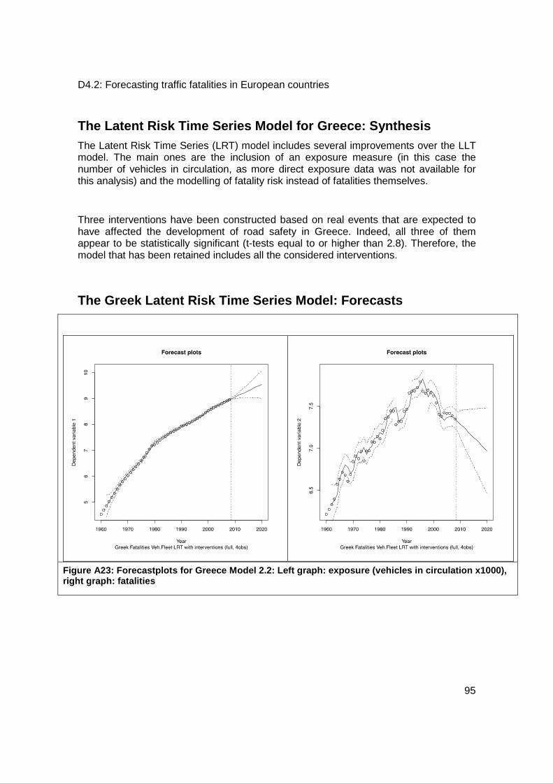
D4.2: Forecasting traffic fatalities in European countries
95
The Latent Risk Time Series Model for Greece: Synth esis The Latent Risk Time Series (LRT) model includes several improvements over the LLT model. The main ones are the inclusion of an exposure measure (in this case the number of vehicles in circulation, as more direct exposure data was not available for this analysis) and the modelling of fatality risk instead of fatalities themselves.
Three interventions have been constructed based on real events that are expected to have affected the development of road safety in Greece. Indeed, all three of them appear to be statistically significant (t-tests equal to or higher than 2.8). Therefore, the model that has been retained includes all the considered interventions.
The Greek Latent Risk Time Series Model: Forecasts
Figure A23: Forecastplots for Greece Model 2.2: Lef t graph: exposure (vehicles in circulation x1000), right graph: fatalities

Appendix A – Detailed results
96
Final model Greece – Latent Risk Model (with interv entions) – Forecasts
Exposure (vehicles in circulation x1000) Fatalities
Year Forecasted
value Lower limit Upper limit Forecasted
number Lower limit Upper
limit
2009 8130.2 7824.0 8448.3 1505 1344 1686
2010 8542.1 8003.0 9117.6 1458 1244 1710
2011 8975.0 8143.1 9891.9 1413 1158 1724
2012 9429.8 8249.9 10778.4 1369 1081 1733
2013 9907.6 8326.4 11789.1 1326 1011 1739
2014 10409.7 8374.8 12939.0 1285 946 1744
2015 10937.2 8396.8 14246.2 1245 886 1748
2016 11491.4 8393.9 15732.0 1206 830 1751
2017 12073.7 8367.6 17421.4 1168 778 1754
2018 12685.5 8319.3 19343.4 1132 729 1757
2019 13328.4 8250.4 21531.8 1097 684 1759
2020 14003.8 8162.3 24025.8 1062 641 1762
Note: The upper and the lower limit define the conf idence interval in which the values lie with 95% chance if the present trend is continued
.

D4.2: Forecasting traffic fatalities in European countries
97
A.4 RESULTS ITALY
A.4.1 Raw data
Figure A24: Exposure (Number of vehicles for Italy, 1980 to 2008; total number of observations in the series: 29).
Figure A25: Fatalities (30 days for Italy from 1999: 1980 to 2008; total number of observations in the series: 29).
A.4.2 Italy: Univariate Model (LLT) of Fatalities - Version StateSpaceIncludes.R: dlm 0.6.3 22/10/2010
- Models run on: 3/11/2010
Model quality Model 1.1 -
Stochastic level and slope
Model 1.2 – With fixed slope
Model 1.3 - With fixed level
Model 1.4 – With fixed level and
slope Log-Likelihood 47.644 47.865 45.878 35.628
AIC -95.080 -95.592 -91.619 -71.187
Residuals (Prediction Errors)
Box-Ljung Lag 3 ns ns ns 0.0002

Appendix A – Detailed results
98
Lag 4 ns ns ns 0.0006 Lag 5 ns ns ns 0.0003 Heteroscedasticity ns ns ns 0.0002 Normality ns ns ns ns Auxiliary residuals: Output : ns ns ns ns Level : 0.039 0.045 0.051 ns Slope : ns ns ns ns Model prediction MPE4 -1.27 -1.24 0.093 -1.68 MAPE4 1.27 1.24 0.177 1.68 MPE7 -2.44 -1.91 -4.47 -0.51 MAPE7 2.44 1.91 4.47 1.06 MPE10 1.79 1.83 2.43 0.96 MAPE10 1.81 1.84 2.43 1.31 Table A14 Diagnostic tests for Italian local linear trend models
Model dynamics Model 1.1 -
Stochastic level and slope
Model 1.2 – With Fixed Slope
Model 1.3 - With Fixed level
Model 1.4 – With fixed level and
slope Observation errors
2εσ
1.06E-11 5,05E-07 - 3.2 E-03
2.81E-05 3.22E-05- 2.05E-01
9.3 E-04 2.4 E-04 - 2.0 E-03
6.2 E-03 3.3 E-03- 1.0 E-02
Level disturbances 2ξσ
3.1E-03 1.6E-03 - 5.3E-03
0.003.3 E-03 0.001.9 E-03 -
0.005.4 E-03
/ /
Slope disturbances 2ζσ
1.08E-11 5.21E-07 - 3.2 E-03
/ 1.1 E-03 1.1 E-04- 3.0 E-03
/
Table A15 Model dynamics for Italian local linear t rend models

D4.2: Forecasting traffic fatalities in European countries
99
Figure A26: Smoothed state plots for Italy Model 1. 1: Left-hand graph: Trend; right-hand graph: Slope
The Local Linear Trend Model for Italy: Synthesis Residuals and prediction errors (Table A14) show that the development of Italian fatalities are well represented by the LLT model with stochastic level and slope. There are just some marginally significant results in level auxiliary residuals but they are quite near the 5% chance to become significant, and there is no reason to doubt that the model behaves well. The LLT model with fixed slope has equal results, while the model with fixed level and stochastic slope shows just a small decrease in the log-likelihood. When both level and slope components are fixed there are some problems of autocorrelation and log-likelihood statistics and Akaike criterion worsen. The general trend of fatalities is decreasing. The slope is slightly negative and vey strangely constant through the series. The smoothed state plot of trend shows a strong increase in the number of fatalities in correspondence of years 1991 and 1999.
A.4.3 Italy: bivariate model (LRT) of fatalities an d exposure
Data and interventions in Italy The existing data gathering survey in Italy is based on form and survey methods introduced by the Italian Institute of Statistic (ISTAT) in 1991. Official ISTAT data about injury crashes starts from this year; before 1991, ISTAT gathered data for all crash gravity. Another important date for crash data collection is 1999, when ISTAT extended the time period used for the definition of a road crash fatality from 7 days to 30 days.

Appendix A – Detailed results
100
Number of vehicles has been used for exposure measure, no relevant changes in reporting methods occurred during the period of study. There have been a number of events and interventions in the considered period that could affect the number of fatalities. Not all of them were considered for LRT model development, since for some of them a significant change in fatalities was not observed (e.g., seatbelt obligation in 1988, penalty point system in 2003). Years of considered events/interventions are: 1986: Safety helmet obligation. It has been considered through a level intervention on the risk. 1991: Change in road crash data collection introduced by ISTAT. It has been included in the model as explanatory variable. 1992: New Highway Code was introduced in Italy. It’s possible to see a decrease in 1993 in the number of fatalities. It has been considered through a level intervention on the risk. 1999: Change in the way of recording fatalities (from killed 7 days to killed 30 days). It has been included in the model as explanatory variable.
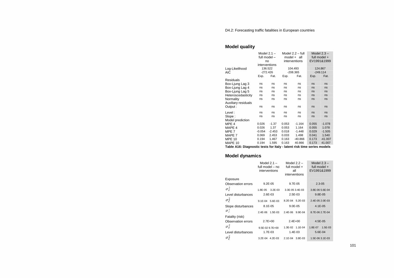
D4.2: Forecasting traffic fatalities in European countries
101
Model quality Model 2.1 –
full model – no
interventions
Model 2.2 – full model + all interventions
Model 2.3 – full model +
EV1991&1999
Log-Likelihood 136.522 104.493 124.867 AIC -272.426 -208.365 -249.114 Exp. Fat. Exp. Fat. Exp. Fat. Residuals Box-Ljung Lag 3 ns ns ns ns ns ns Box-Ljung Lag 4 ns ns ns ns ns ns Box-Ljung Lag 5 ns ns ns ns ns ns Heteroscedasticity ns ns ns ns ns ns Normality ns ns ns ns ns ns Auxiliary residuals Output : ns ns ns ns ns ns
Level : ns ns ns ns ns ns Slope : ns ns ns ns ns ns Model prediction MPE 4 0.026 -1.37 0.053 -1.164 0.055 -1.078 MAPE 4 0.026 1.37 0.053 1.164 0.055 1.078 MPE 7 -0.054 -2.453 0.018 -1.448 0.029 -1.505 MAPE 7 0.069 2.453 0.033 1.498 0.041 1.540 MPE 10 0.194 1.467 0.163 -40.866 0.173 -41.007 MAPE 10 0.194 1.595 0.163 40.866 0.173 41.007 Table A16: Diagnostic tests for Italy - latent risk time series models
Model dynamics Model 2.1 –
full model – no interventions
Model 2.2 – full model +
all interventions
Model 2.3 – full model +
EV1991&1999
Exposure
Observation errors 2εσ
9.2E-05
1.8E-05 3.2E-03
9.7E-05
3.3E-05 3.4E-03
2.3-05
3.8E-06 5.6E-04
Level disturbances 2ξσ
2.6E-03
9.1E-04 5.6E-03
2.5E-03
8.2E-04 5.2E-03
9.8E-05
2.4E-05 2.0E-03
Slope disturbances 2ζσ
8.1E-05
2.4E-06 1.5E-03
9.0E-05
2.4E-06 9.9E-04
4.1E-05
8.7E-06 2.7E-04
Fatality (risk)
Observation errors 2εσ
2.7E+00
9.5E-02 9.7E+00
2.4E+00
1.3E-02 1.1E-04
4.5E-05
1.8E-07 1.5E-03
Level disturbances 2ξσ
1.7E-03
3.2E-04 4.2E-03
1.4E-03
2.1E-04 3.8E-03
5.6E-04
1.5E-06 3.1E-03

Appendix A – Detailed results
102
Slope disturbances 2ζσ
1.3E-04
6.5E-02 8.2E-04
1.5E-04
1.2E-0 6 6.3E-04
1.1E-04
2.3E-07 4.7E-04
Intervention1 (Explanatory variable)
(1991) tβ
1.6 E-02
-1.4E-01*
Intervention2 (Explanatory variable)
(1999) tβ
3.5E-03 -1.3E-01*
Intervention3
(1986) tβ
2.7E-03
Intervention2
(1992) tβ
6.0 E-03
Table A17 Model dynamics for Italy - latent risk ti me series models
Selected model for Italy: Model 2.3 LRT full model with Interventions 1991 and 1999

D4.2: Forecasting traffic fatalities in European countries
103
.
Figure A27: Smoothed output plots for Italy Model 2 .3: left: exposure, right: fatalities
Figure A28: Smooth state plots for Italy Model 2.3: Upper left: Trend exposure, upper right: trend fatality risk, lower left: slope expos ure, lower right: slope fatality risk

Appendix A – Detailed results
104
The Latent Risk Time Series Model for Italy: Synthe sis Main characteristics of LRT models developed for the Italian case are shown in Table A16. Three different models have been tested:
• a stochastic model without interventions (Model 2.1), • a stochastic model with all interventions included, both crash data gathering
related interventions and road safety related interventions (Model 2.2), • a stochastic model including only changes in crash data gathering process
(Model 2.3).
Results show that the three models behave well; no significant values in the residual tests were reported (Table A16). However none of the interventions included in Model 2.2 became significant, while when considering only interventions in 1991 and 1999 as a dummy explanatory variable (Model 2.3) interventions result significant. Therefore Model 2.3 has been chosen as it behaves better in explaining past interventions.
Figure A27 and Figure A28 show the smoothed output plots and smoothed state plots for Model 2.3. Looking at output and state plots of the exposure trend it can be seen that they are very similar. In contrast, the fatality development (output) has a different trend compared to the fatality risk development (state). The increased number of fatalities highlighted in the output plot in the beginning and at the end of 1990s is smoothed down in the fatality risk plot.
The Italian Latent Risk Time Series Model: Forecast s
Figure A29: Forecastplots for Italy Model 2.3: Left graph: exposure, right graph: fatalities

D4.2: Forecasting traffic fatalities in European countries
105
Final model Italy – Latent Risk Model 2.3 with all Interventions – Forecasts
Exposure (vehicles) Fatalities
Year Estimated value
Lower limit
Upper limit
Estimated number
Lower limit
Upper limit
2009 49137743 47649834 50672114 4518 4161 4905
2010 50401627 47932529 52997914 4289 3795 4848
2011 51698019 48096336 55569414 4072 3466 4786
2012 53027756 48141713 58409698 3866 3163 4727
2013 54391696 48075859 61537259 3671 2883 4674
2014 55790718 47906738 64972159 3485 2624 4629
2015 57225724 47641999 68737324 3309 2385 4591
2016 58697641 47288813 72858945 3142 2164 4561
2017 60207417 46853913 77366708 2983 1960 4538
2018 61756026 46343660 82294035 2832 1773 4523
Note: The upper and the lower limit define the confidence interval in which the values lie with 95% chance if the present trend is continued.

Appendix A – Detailed results
106
A.5 RESULTS UNITED KINGDOM
A.5.1 Raw data The data used in the modelling are the annual numbers of fatalities and the vehicle kilometres (traffic) for Great Britain and Northern Ireland, added together to give UK. The traffic and fatality data are available for Great Britain from 1947 but for Northern Ireland the traffic data are only available from 1991.
Initially models were fitted to the UK data from 1991. It was subsequently decided that better fitting models could be developed using a longer time series. The example presented here uses data from 1983. This start year was chosen to minimise any effects of the compulsory wearing of seatbelts law introduced at the start of 1983 and to minimise the number of traffic data that would need to be imputed for Northern Ireland (8 years).
Time
UK
traffi
c
1985 1990 1995 2000 2005 2010
420
440
460
480
500
520
Time
UK
fat
1985 1990 1995 2000 2005 2010
2500
3000
3500
4000
4500
5000
5500
Figure A30: Exposure (Vehicle kilometres) for the UK, 1991 to 2009; total number of observations in the series:19.
Figure A31: Fatalities for the UK, 1983 to 2009; total number of observations in the series:27.
A.5.2 UK: Univariate Model of Fatalities (LLT) • Version StateSpaceIncludes.R: 25/10/2010
• DaCoTAStateSpaceIncludes version: dlm 0.6.3 22/10/2010

D4.2: Forecasting traffic fatalities in European countries
107
• Models run on: 23/11/2010
Model quality
Model 1.1 - Stochastic level
and slope
Model 1.2 – With fixed slope
Model 1.3 - With fixed level
Model 1.4 – With fixed level and
slope
Log-Likelihood 45.1957 44.0731 44.8654 32.459 AIC -90.1693 -87.998 -89.5827 -64.8439
Residuals
(Prediction Errors)
Box-Ljung Lag 3 n.s n.s n.s 0.000 Lag 4 n.s n.s n.s 0.000 Lag 5 n.s n.s n.s 0.000
Heteroscedasticity n.s n.s n.s n.s Normality n.s n.s n.s n.s
Auxiliary residuals: Output : n.s n.s n.s n.s Level : n.s n.s n.s n.s Slope : n.s n.s n.s n.s
Model prediction MPE4 -1.42 -1.41932 -1.17151 -0.578878
MAPE4 1.50 1.50178 1.3027 1.2024 MPE7 -0.723 -0.722808 -1.98902 0.668501
MAPE7 0.956 0.95598 2.05829 1.23833 MPE10 0.697 0.696668 -0.110414 1.50313
MAPE10 1.132 1.132 0.931608 1.60135 Table A18 Diagnostic tests for UK fatalities local linear trend model

Appendix A – Detailed results
108
State Auxiliary Residuals
UK fatals local linear trend model (full)Year
Leve
l
1985 1990 1995 2000 2005 2010
-2-1
01
2
State Auxiliary Residuals
UK fatals local linear trend model (full)Year
slop
e
1985 1990 1995 2000 2005 2010
-2-1
01
2
Figure A32: State (level) auxiliary residuals for UK Model 1.1
Figure A33: State (slope) auxiliary residuals for UK Model 1.1
State Auxiliary Residuals
UK fatals local linear trend model (fixed level)Year
Leve
l
1985 1990 1995 2000 2005 2010
-2-1
01
2
State Auxiliary Residuals
UK fatals local linear trend model (fixed slope)Year
slop
e
1985 1990 1995 2000 2005 2010
-2-1
01
2
Figure A34: State (level) auxiliary residuals for UK Model 1.2
: Figure A35: State (slope) auxiliary residuals for UK Model 1.3

D4.2: Forecasting traffic fatalities in European countries
109
Model dynamics Model 1.1 -
Stochastic level and slope
Model 1.2 – With Fixed Slope
Model 1.3 - With Fixed level
Model 1.4 – With fixed level
and slope Observation errors
2εσ
1.85861e-12
0.0000012, 0.0048
8.22978e-13
2.35e-07, 0.00115
0.000344
1.525e-05, 0.00114
0.00563615
0.00286, 0.00935 Level disturbances
2ξσ
0.00129781
0.00016, 0.0034
0.00281206
0.00136, 0.00459
0 (fixed) 0 (fixed)
Slope disturbances 2ζσ
0.0006351
0.0000122, 0.0025
0 (fixed) 0.00115562
0.000181, 0.00301
0 (fixed)
Table A19 UK: Model dynamics for local linear trend models
Smoothed state plots
UK fatals local linear trend model (full)Year
Leve
l
1985 1990 1995 2000 2005 2010
7.8
8.0
8.2
8.4
8.6
Smoothed state plots
UK fatals local linear trend model (full)Year
slop
e
1985 1990 1995 2000 2005 2010
-0.1
5-0
.10
-0.0
50.
00
Figure A36: Smoothed state plot for UK Model 1.1
Figure A37: Smoothed state plot for slope for UK Model 1.1
Local Linear Trend Model for UK: model synthesis The local linear trend model was fitted including no explanatory variables or interventions. The model assumptions were satisfied. The auxiliary residuals were inspected for outliers, slope and level breaks. The plot of the level auxiliary residuals (Figure A32) suggests a possible level break between 1989 and 1991 and the plot of the slope auxiliary residuals (Figure A33) suggest possible slope break in 1990 and 2006. These changes in pattern are

Appendix A – Detailed results
110
around the times of the two economic recessions in the UK. However when traffic is added as an explanatory variable the possible slope break in 1990 is explained although traffic does not fully explain the large drops in fatalities in 2006. The variance of the slope in model 1.1 is small. When treated as a deterministic effect the log likelihood reduces only slightly from 45.2 to 44.1 and the model prediction errors are the same as the full model. However descriptively the slope does vary, as it is negative in the early 1990’s and from 2006 at the times of the two recessions and not significantly different from zero in between. Consequently, model 1.2 does not adequately describe the series after 2003 (Figure A34). There is a level break in model 1.3 between 1989 and 1991 (the previous recession). Without traffic as an explanatory variable these models do not satisfactorily predict fatalities in the UK. When traffic is added as a fixed and known parameter the level can be treated as deterministic (fixed).
A.5.3 UK: bivariate model (LRT) of fatalities and exposure In the previous analysis it was established that traffic was a significant explanatory variable and that the level term could be treated as a deterministic component when traffic is added. The next step was to fit a latent risk time series (LRT) model to the UK data. This approach allows the explanatory variable to have error by adding it to the model as a second dependent variable. The latent risk time series (LRT) model is a bivariate local linear trend model with two observation equations and four state equations. The explanatory variable (traffic) is now treated stochastically and the observation disturbances, level disturbances and slope disturbances are allowed to be correlated.
• Version StateSpaceIncludes.R: 25/10/2010
• DaCoTAStateSpaceIncludes version: dlm 0.6.3 22/10/2010
• Models run on: 24/11/2010
We have the fatality data for the UK from 1983 but the traffic data is only available from 1991. Therefore the latent risk model with the traffic data included as an extra dependent variable with missing values from 1983-1990 was run for the UK. The model estimated values for the traffic data prior to 1991.
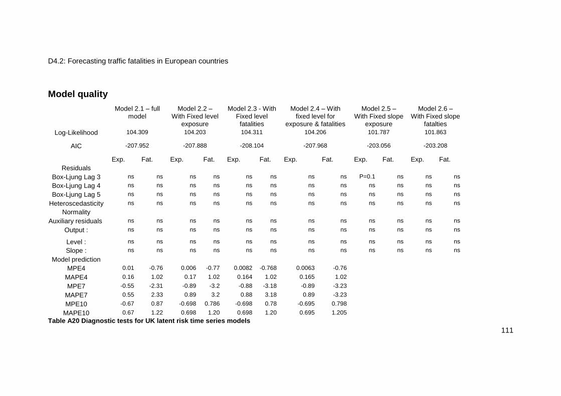
D4.2: Forecasting traffic fatalities in European countries
111
Model quality Model 2.1 – full
model Model 2.2 –
With Fixed level exposure
Model 2.3 - With Fixed level
fatalities
Model 2.4 – With fixed level for
exposure & fatalities
Model 2.5 – With Fixed slope
exposure
Model 2.6 – With Fixed slope
fatalties Log-Likelihood 104.309 104.203 104.311 104.206 101.787 101.863
AIC -207.952 -207.888 -208.104 -207.968 -203.056 -203.208
Exp. Fat. Exp. Fat. Exp. Fat. Exp. Fat. Exp. Fat. Exp. Fat. Residuals
Box-Ljung Lag 3 ns ns ns ns ns ns ns ns P=0.1 ns ns ns
Box-Ljung Lag 4 ns ns ns ns ns ns ns ns ns ns ns ns
Box-Ljung Lag 5 ns ns ns ns ns ns ns ns ns ns ns ns
Heteroscedasticity ns ns ns ns ns ns ns ns ns ns ns ns
Normality
Auxiliary residuals ns ns ns ns ns ns ns ns ns ns ns ns
Output : ns ns ns ns ns ns ns ns ns ns ns ns
Level : ns ns ns ns ns ns ns ns ns ns ns ns
Slope : ns ns ns ns ns ns ns ns ns ns ns ns
Model prediction
MPE4 0.01 -0.76 0.006 -0.77 0.0082 -0.768 0.0063 -0.76
MAPE4 0.16 1.02 0.17 1.02 0.164 1.02 0.165 1.02
MPE7 -0.55 -2.31 -0.89 -3.2 -0.88 -3.18 -0.89 -3.23
MAPE7 0.55 2.33 0.89 3.2 0.88 3.18 0.89 -3.23
MPE10 -0.67 0.87 -0.698 0.786 -0.698 0.78 -0.695 0.798
MAPE10 0.67 1.22 0.698 1.20 0.698 1.20 0.695 1.205 Table A20 Diagnostic tests for UK latent risk time series models

Appendix A – Detailed results
112
Model dynamics
Model 3.1 – Full model
Model 2.2 – With Fixed
level exposure
Model 2.3 - With Fixed
level fatalities
Model 2.4 – With fixed level for exposure &
fatalities
Model 2.5 – With Fixed slope
exposure
Model 2.6 – With Fixed slope fatalties
Exposure
Observation errors 2εσ
7.1e-06 (1.1e-06, 0.0003)
1.2e-05 (3.6e-06, 7.5e-05)
6.7e-06 (5.6e-07, 9.9e-05)
1.2e-05 (2.5e-06, 8.3e-05)
4.8e-06 (7.4e-07, 0.0001)
8.4e-06 (1.57e-06, 0.000195)
Level disturbances 2ξσ
2.27e-05 (7.07e-06, 0.0016)
FIXED 2.4e-05 (1.27e-07, 0.0002)
FIXED 0.000124 (6.9e-05, 0.00051)
8.99e-05 (2.99e-05, 0.00047)
Slope disturbances 2ζσ
4.5e-05 (1.47e-06, 0.0003)
6.0e-05 (1.6e-05, 0.00014)
4.4e-05 (5.6e-06, 0.0001)
6.0e-05 (1.8e-05, 0.0001)
FIXED 3.9e-06 (1.49e-08, 4.9e-5)
Fatality (risk)
Observation errors 2εσ
0.000257 (2.1e-06, 0.00094)
0.0002 (7.3e-06, 0.00073)
0.00026 (1.1e-05, 0.0008)
0.000239 (1.0e-05, 0.00076)
0.000121 (3.1e-07, 0.001)
3.9e-05 (2.2e-07, 0.00087)
Level disturbances 2ξσ
1.7e-07 (5.31e-07, 0.004)
1.4e-06 (9.4e-07, 0.0051)
FIXED FIXED 0.00088 (7.1e-05, 0.0025)
0.0019 (0.0009, 0.003)
Slope disturbances 2ζσ
0.000933192 (2.2e-05, 0.003)
0.00097 (0.00026, 0.0020)
0.00091 (0.00024, 0.0020)
0.001 (0.00028, 0.00202)
0.00024 (2.7e-05, 0.0007)
FIXED
Table A21 Model dynamics for UK - latent risk time series models

D4.2: Forecasting traffic fatalities in European countries
113
Smoothed output plots
Year
Dep
ende
nt v
aria
ble
1
UK fatals and traffic latent risk model
1985 1990 1995 2000 2005 2010
5.9
6.0
6.1
6.2
Smoothed output plots
YearD
epen
dent
var
iabl
e 2
UK fatals and traffic latent risk model
1985 1990 1995 2000 2005 2010
7.8
8.0
8.2
8.4
8.6
Figure A38 : Smoothed output plot (exposure) for UK Model 2.1
Figure A39: Smoothed output plot (fatalities)for UK Model 2.1
Smoothed state plots
UK fatals and traffic latent risk modelYear
Leve
l exp
osur
e
1985 1990 1995 2000 2005 2010
5.9
6.0
6.1
6.2
Smoothed state plots
UK fatals and traffic latent risk modelYear
Lev
el ri
sk
1985 1990 1995 2000 2005 2010
1.4
1.6
1.8
2.0
2.2
2.4
2.6
Figure A40: Smoothed state plot for UK Model 2.1- trend exposure
Figure A41: Smoothed state plot for UK Model 2.1- trend fatality risk

Appendix A – Detailed results
114
Smoothed state plots
UK fatals and traffic latent risk modelYear
slop
e ex
posu
re
1985 1990 1995 2000 2005 2010
-0.0
2-0
.01
0.00
0.01
0.02
Smoothed state plots
UK fatals and traffic latent risk modelYear
slop
e ris
k1985 1990 1995 2000 2005 2010
-0.2
0-0
.15
-0.1
0-0
.05
0.00
Figure A42: Smoothed state plot for UK Model 2.1 - slope exposure
Figure A43: Smoothed state plot for UK Model 2.1- slope fatality risk
Latent Risk Time series Model for UK: synthesis The number of people killed has varied fairly erratically, with periods of slow decline in 1983-1990 and 1996-2003 separated by a period of more rapid decline between 1991 and 1995 and 2007 to 2009 (Figure 39). Figure 41 shows how the fatality risk per billion (109) vehicles KM has developed in the UK between 1983 and 2009. It can be seen that overall the UK fatality risk has been declining for many years. The effects of the two recessions (periods of economic decline) in the early 1990s and in 2007 appear to have influenced the gradient of the risk curve, with it declining more steeply during these periods.
The analysis in Table A20 suggests that the level should be fixed for both exposure and fatalities with the log likelihood criteria showing little difference from the full model. This is in agreement with the univariate analysis when traffic was added as an explanatory variable.
The smooth state plots of slope exposure and fatality risk suggest that the slope term should not be fixed and is better when modelled stochastically. When these elements are fixed the log likelihood criteria is smaller.
The forecasts for the full LRT model and for the model with the level for exposure and fatalities fixed are very similar forecasts which supports treating the level component as deterministic.

D4.2: Forecasting traffic fatalities in European countries
115
The Latent Risk Time Series Model (full model) for UK: Forecasts for UK
Forecast plots
Year
Dep
ende
nt v
aria
ble
1
UK fatals and traffic latent risk model
1985 1990 1995 2000 2005 2010 2015 2020
5.9
6.0
6.1
6.2
6.3
6.4
Forecast plots
Year
Dep
ende
nt v
aria
ble
2
UK fatals and traffic latent risk model
1985 1990 1995 2000 2005 2010 2015 2020
56
78
Figure A44: Traffic forecasts for the UK (based on full LRT model)
Figure A45 : Fatality forecasts for the UK (based on full LRT model)
Latent Risk Model for the UK (full model) – Forecasts
Exposure (vehicle kms / million) Fatalities
Year Estimated value
Lower limit Upper limit Estimated number
Lower limit Upper limit
2010 520 510 530 2035 1830 2262
2011 516 497 535 1773 1458 2156
2012 512 483 542 1545 1137 2100
2013 508 468 551 1346 871 2080
2014 504 453 562 1173 658 2092
2015 501 436 574 1022 491 2131
2016 497 420 588 891 361 2198
2017 493 403 603 776 263 2293
2018 489 386 620 677 189 2418
2019 486 369 639 590 135 2575

Appendix A – Detailed results
116
2020 482 352 659 514 95 2768
Note: The upper and the lower limit define the confidence interval in which the values lie with 95% chance if the present trend is continued.
The Latent Risk Time Series Model (fatality and exp osure level fixed): Forecasts for UK
Forecast plots
Year
Dep
ende
nt v
aria
ble
1
UK fatals and traffic latent risk model fixed level - fatalities & exposure
1990 2000 2010 2020
5.8
5.9
6.0
6.1
6.2
6.3
6.4
6.5
Forecast plots
Year
Dep
ende
nt v
aria
ble
2
UK fatals and traffic latent risk model fixed level - fatalities & exposure
1990 2000 2010 2020
56
78
Figure A46: Traffic forecasts for the UK (based on LRT model with fixed level for fatalities and exposure)
Figure A47 : Fatality forecasts for the UK (based on LRT model with fixed level for fatalities and exposure)
Latent Risk Model for the UK (fixed level for exposure and fatalities ) – Forecasts
Exposure (vehicle kms / million) Fatalities
Year Estimated value
Lower limit Upper limit Estimated number
Lower limit Upper limit
2010 519 509 530 2033 1834 2254
2011 515 496 535 1770 1458 2149
2012 511 481 543 1541 1132 2096
2013 506 464 553 1341 864 2082
2014 502 447 565 1168 649 2101
2015 498 429 578 1016 481 2149

D4.2: Forecasting traffic fatalities in European countries
117
2016 494 411 594 885 351 2227
2017 490 392 612 770 254 2335
2018 486 374 631 670 182 2476
2019 482 355 653 584 128 2653
2020 478 337 676 508 90 2872

Appendix B – Instructions for analyses
118
APPENDIX B: INSTRUCTIONS FOR ANALYSES
In this appendix the instructions to conduct the analyses reported above are given. In the first section the general steps to be taken are outlined, in the second section the template that was filled in for each country analysed is given, and in the third section a practical instruction how to run the analysis in R is included.

D4.2: Forecasting traffic fatalities in European countries
119
B.1 MAJOR STEPS IN THE ANALYSES:
B.1.1 Investigating the univariate model: The essential of the work at this step consist of investigating what are the components in the state of the fatality series that should be treated stochastically. Starting with the “full” Local Linear Trend model, we obtain estimates of the variances of the disturbances of the different state components (transition covariance matrix Q). It is however not evident to evaluate what disturbances are “small”, and what are “large”. It is therefore necessary to run additional versions of the LLT while treating one component as fixed, and comparing this “restricted” model to the full one on the basis of the log-likelihood and AIC, but also on the basis of the results of the residual tests is therefore necessary. Of course, if the results are disastrous (i.e.: sharp decrease of log-likelihood value, autocorrelated residuals…) once one of the components is fixed, there is no use in testing a version of the model where all components are treated deterministically.
B.1.2 Step 2: Investigating the bivariate model. In the following, we will describe a number of investigation steps that will help us understanding the dynamic structure in more detail on the one hand, and on the other hand, to specify a model that is tailored to the country in question.
We suggest to first check whether you need to include interventions into the model and then whether certain levels or slopes in the model can be fixed. This order is meant as a guideline, however, and it might in some cases be necessary to change the order (e.g. an intervention could be non-significant with a stochastic slope but become significant if it is fixed).
B.1.3 Identifying Interventions Interventions are structural breaks that are specified in the model and therefore are taken out of the “normal dynamics” because they are thought to be of a different nature. It is important to realize that whatever is specified as an intervention does therefore not anymore form the basis of forecasting future developments.
We are working with yearly, national data: candidates for interventions should consequently be measures that have been adopted at the national level and concern the majority of road users.
There are three main possibilities with respect to the form that can be given to the intervention:
- You suspect that some change in the series reflects a change in the way it has been measured and not a change in the phenomenon itself. Such changes should be implemented in the measurement equation. The necessity to

Appendix B – Instructions for analyses
120
implement such an intervention would be indicated by an extreme value in the output auxiliary residuals. There are two different options
o The measurement of either variable (fatalities or exposure) was temporarily corrupted. You think that the fatality number or the exposure for a particular year (or for a number of years) is for some reason an over- or underestimation of the real value. Theoretically, one could define a pulse- intervention on the measurement equation here, but practically it amounts to the same as defining the flawed number as a missing value (which is much easier to do, just replace the value with “NA”).
o The measurement of fatalities or exposure has changed in a durable way. The typical example is a change in the registration of fatalities (e.g. the switch from killed 7 days to killed 30 days). Such permanent changes to the measurement should be reflected by an intervention in the measurement equation. To do this, you have to define a “dummy variable”, which is 1 for all years before the registration change and 0 for all years since and use it as an explanatory variable (see Section 3.2.3.11 for a detailed instruction).
- Some measure has caused a permanent reduction in either the fatality-risk
(e.g., seat-belt law) or in the exposure (e.g. introduction of taxes). Such interventions can be identified on the basis of the state auxiliary residuals (in this case the level) and should be included in the level-equations for either exposure or the fatality risk. A level intervention takes the form of a step. At the moment of the intervention the risk is increased or decreased and afterwards it stays that way without any further changes. Of course this does not mean that after the intervention there should not be any changes in the component in question any more, but these changes should be comparable in size and direction to those before the intervention. Such an intervention is included with the “interventions” option into the level (component 1 for exposure and component 3 for fatality risk, see Section 3.2.3.10)
- Something caused a change of direction in the development of either fatality
risk or mobility. The need for such interventions can be identified in the state auxiliary residuals (in this case for the slope). A reason for such a change in direction could, for example, be an increased commitment in a country to improve road-safety due to which the fatality risk decreases at a faster rate than before. Such changes in direction have to be implemented as slope interventions (use the intervention function with component 2 for exposure and component 4 for fatality risk). In practice interventions to the slope are very rare however.
The selection of “candidates for interventions” should be based on the results of the analyses of the auxiliary residuals (values <-2 or >2), as well as on knowledge of the measures that have been adopted to improve RS in the country analysed. Keep in mind that interventions (or missing values) that are implemented when the time-series show extreme values or changes reduce the error variance and consequently the confidence interval for the forecasts. This is a good thing if you have reasons to

D4.2: Forecasting traffic fatalities in European countries
121
assume that no such changes will occur in the future. However, if we do not really understand the reasons for the changes in the past, we have no reason to expect that they won’t occur in the future as well. In that case, correcting our models for the past “quirks” by introducing interventions would artificially reduce the confidence intervals for our forecasts.
The codes for the inclusion of interventions in the model are presented in Sections 3.2.3.9 and 3.2.3.10.
B.1.4 Fixing components As described above, the bivariate model contains four state components: The mobility level, the mobility slope, the fatality-risk level and the fatality risk-slope. Each of these has their own disturbances, which allow the components to vary from one time-point to the next.
The models can be simplified by fixing components, i.e. by forcing the disturbance variance to be zero. The component becomes deterministic instead of stochastic.
Check for each of the components whether they can be fixed. Try fixing the components. Consider their significance which is now given in the form of simulations of the upper and lower percentiles of the distribution of the disturbances (see Section 3.3.1.3). If the confidence interval does not contain zero, the component is significant. You should, however, not solely rely on the results of these significance tests. Check whether the graphs seem to suggest the same conclusion. And compare the model with the component fixed to the full model. A component should certainly not be fixed if that results in problems with the residual tests. In case of doubt, we advise to leave a component stochastic rather than fixing it, as there are no strong disadvantages to not fixing a component.

Appendix B – Instructions for analyses
122
B.2 TEMPLATE
B.2.1 Raw data
Insert a raw plot of the fatality series in this table
Figure 1: Fatalities (30 days, 24 days, “on the spot…” for Belgium, France… 19xx to 20xx; total number of observations in the series: xx)
Insert a raw plot of the exposure series in this table
Figure 2: Exposure (“Vehicle kilometres, Number of Vehicles…” for Belgium, France… 19xx to 20xx; total number of observations in the series: xx)
B.2.2 Step 1 Univariate Model (LLT) of Fatalities: - For all certainty: Mention the version of the “StateSpaceIncludes.R” that has been used (reported in the text output) and the date upon which the model has been run…
Model quality Report values for the log-likelihood and AIC, for the residual tests: report the p-value if the test is significant, but otherwise simply “n.s.”, for the normality tests (residuals and auxiliary residuals), p-value, skewness and kurtosis value if the test is significant, but otherwise simply “n.s”
Model 1 – Local Linear Trend Model - diagnostic tes ts Model 1.1 - Stochastic
level and slope Model 1.2 – With
fixed slope Model 1.3 - With
Fixed level
Log-Likelihood AIC
Residuals
(Prediction Errors)
Box-Ljung Lag xx Lag xx Lag xx
Heteroscedasticity Normality
Auxiliary residuals:

D4.2: Forecasting traffic fatalities in European countries
123
Output : Level : Slope :
Model prediction MPE
MAPE
If the full model has significant values in the residual tests, please include a plot of the residuals in question.
e.g.: Figure X: Standardised Residuals for Model 1.1 (or 1.2..)
Figure X: State (level) auxiliary residuals for Model 1.1 (or 1.2, or…)
Model dynamics Indicate the value and confidence intervals10 for the hyperparameters. The observation errors are given in matrix H (see Section 3.3.1.5) and the state disturbances in matrix Q (see Section 3.3.1.3).
Model 1 – Local Linear Trend Model - Hyperparameter s and parameters
Model 1.1 - Stochastic level and
slope
Model 1.2 – With Fixed Slope
Model 1.3 - With Fixed level
Observation errors 2εσ
Level disturbances 2ξσ
/
Slope disturbances 2ζσ
/
Insert the smoothed state plots for the trend…
… and for the slope here
Figure X: Smoothed state plots for Model 1.1: Left-hand graph: Trend; right-hand graph: Slope
10 Please bear in mind that the significance test for the state disturbances should be considered only as a rough indication

Appendix B – Instructions for analyses
124
The Local Linear Trend Model: Synthesis - Do we have indication that this model captures the dynamics of the series well
enough? In other words; are the assumptions concerning the residuals satisfied? What are the remaining problems, if any?
- Describe the dynamics in the model (e.g.: the slope is negative throughout the series, but its value is decreasing, indicating that the decrease in the number of fatalities has become weaker over the years).

D4.2: Forecasting traffic fatalities in European countries
125
B.2.3 Step 2: The bivariate (LRT) model
Interventions Give a description and a short-name for all interventions included. Include the shortname in the model titles in the table.
Model quality
Model 2 –Latent Risk Model with interventions - dia gnostic tests Model 2.1 – All
stochastic components – All candidates
interventions
Model 2.2 – Model 2.3 -
Log-Likelihood
AIC Exposure Fatalities Exposure Fatalities Exposure Fatalities
Residuals (Prediction Errors)
Box-Ljung Lag xx Lag xx Lag xx
Heteroscedasticity Normality
Auxiliary residuals : Output : Level : Slope :
Model prediction MPE
MAPE
If the full model has significant values in the residual tests, please include a plot of the residuals in question and possibly a plot that gives more information (e.g., autocorrelation functions of the affected state (type DaCoTA.standardisedResidualACFplots (YourModelName) ) if the Box-Ljung test is significant or a QQ-test ( type (DaCoTA.stateAuxiliaryResidualQQplots
(YourModelName) ) if the heteroscedasticity or normality tests are significant.
e.g.: Figure X: Standardised Residuals for Model 2.1 (or 2.2..)
Figure X: State (level) auxiliary residuals for Model 2.1 (or 2.2, or…)

Appendix B – Instructions for analyses
126
Model dynamics Indicate the value and confidence intervals11 for the hyperparameters. The observation errors are given in matrix H (see Section 3.3.1.5) and the state disturbances in matrix Q (see Section 3.3.1.3).
Model 2 – Latent Risk Model with interventions – Hy perparameters and parameters
Model 2.1 – All stochastic components
– All candidates interventions
Model 2.2 - Model 2.3 -
Exposure Observation errors
2εσ
Level disturbances 2ξσ
Slope disturbances 2ζσ
( Interventions )
tβ
Fatality (risk) Observation errors
2εσ
Level disturbances 2ξσ
Slope disturbances 2ζσ
( Interventions )
tβ
Selected model: Indicate the model that seems the best to you (numb er & descriptive title).
Insert the smooth state plot for trend Slope exposure
11 Please bear in mind that the significance test for the state disturbances should be considered only as a rough indication

D4.2: Forecasting traffic fatalities in European countries
127
exposure
Trend fatality risk Slope fatality risk
Figure X: Smooth state plots for Model 2.1: Upper left: Trend exposure, upper right: slope exposure, lower left: trend fatality risk, lower right: slope fatality risk
The Latent Risk Time Series Model: Synthesis - Do we have indication that this model captures the dynamics of the series well
enough? In other words; are the assumptions concerning the residuals satisfied? What are the remaining problems, if any?
- Describe the dynamics in the model. Compare the dynamics of the fatality risk (fatalities given exposure) with the dynamics of the fatalities as described in the local linear trend model. Relate the changes to the dynamics of the exposure.
- Describe the forecasted development.
The Latent Risk Time Series Model: Forecasts
Insert the exposure forecast plot
Insert the fatality forecast plot
Figure X: Forecastplots for Model 2.1: Upper graph: exposure, lower graph: fatalities
Final model – Latent Risk Model (with interventions ) – Forecasts
Exposure (give measure & unit) Fatalities
Year Estimated value
Lower limit
Upper limit
Estimated number
Lower limit
Upper limit
2009
2010
2011
2012
2013
2014
2015
2016

Appendix B – Instructions for analyses
128
2017
2018
2019
2020
Note: The upper and the lower limit define the confidence interval in which the values lie with 95% chance if the present trend is continued.

D4.2: Forecasting traffic fatalities in European countries
129
B.3 PRACTICAL INFORMATION In this section we are going give practical information to run the model in R and to understand the output. Note that this Section reflects the instruction that was given in October 2010 to the partners who ran the analyses reported in the present deliverable. Note that the program is still in development. Before conducting analyses the most recent version of these instructions should be requested.
This section is not necessarily meant to be read as a whole. Some explanations repeat content from the introduction and some explanations have been given in earlier documents (e.g., the Belgian Example).
While for most of the material in this section you only have to read it on demand, for some sections it might be worth your while to take a look at them, because they concern problems or solutions that occurred with one of the partners and they contain information that has not been presented earlier. These sections are marked in yellow.
All R-input code is presented in courier-8 letters in black (we apologize for the small font size, but it was easier to keep lines intact that way) and R-output is presented in courier-8 letters in blue. In the R-code section (3.2) we have paid special attention to the implementation of interventions (3.2.3.10 and 3.2.3.11) and listed all options of the fitDaCoTAModel function. In the output section we have paid some more attention to explaining what the different matrices contain, including examples of “labeled matrices” (printed in grey letters).
B.3.1 In and output in R
Tinn-R Instead of working in the R-console directly, you might want to try Tinn-R. This is a free editor that Costas advised us to use. It allows you having a whole of R-code (and not just one command-line as in the R-console) and editing it. This is handy, if you want to adapt an existing code. For example, you have received a code from another partner (and thus for another country) and thus have to adjust it in several places (e.g. you have to replace all instances of the word “Belgium” for the name of another country). From Tinn-R you can submit parts (lines, commands) or the complete code to R. We have certainly not discovered all features of Tinn-R, as we just started to use it ourselves, but for us the R-card (found in the left-side of the Tinn-R window) is very handy. The R-card contains R commands ordered by topics that can be directly inserted in the code you are working with by clicking on them. If you use Tinn-R, do not open R via Tinn-R’s menu, because then R does not read the .Rprofile upon opening. Just open R as you always have.

Appendix B – Instructions for analyses
130
Data-file We advise you to have a separate code-file to generate your datafile. It could look somewhat like this
setwd(DaCoTADataDir) BelgiumFAT.dat<- read.delim(paste(DaCoTADataDir,"Belgium/","BelgiumF AT.dat",sep=""),sep="") endYear<-BelgiumFAT.dat[dim(BelgiumFAT.dat)[1],"YEA R"] BelgiumFat<-ts(BelgiumFAT.dat$BelgiumFAT,start=1973,end=endYear ,frequency=1,names=c("Fatalities Belgium")) BelgiumVKMS.dat<- read.delim(paste(DaCoTADataDir,"Belgium/","BelgiumV KM.dat",sep=""),sep="") BelgiumVKMS<-ts(BelgiumVKMS.dat$BelgiumVKM,start=1973,end=endYea r,frequency=1,names=c("Vehicle Kilometrage (million) Belgium"))
For a two-level LRT model you need two time-series that are bound into one object. You have to create such an object with the cbind command. Assuming that exposure is your first level and fatalities the second, you have to put the two variables in exactly that order into the cbind command.
BelgiumTwoLevel <- cbind (BelgiumVKMS, BelgiumFat)
These data have to be saved by the following command.
save.image(paste(DaCoTADataDir,"Belgium.Rdata",sep= ""),ascii=TRUE)
Start your R-session - Set the working directory to the directory you want to put your output in:
setwd(paste(DaCoTACodeDir,"YourSubDirectoryName/",s ep=""))you
- Load the packages that you need:
library (dlm) library (numDeriv)
- Load the data:
load(paste(DaCoTADataDir,"Belgium.Rdata",sep=""))
- And finally, load the DaCoTAStateSpaceIncludes.R file. You should load this after loading the data file, because it turned out that some partners have accidentally saved things in their data that they were not aware of (e.g. functions from older versions of the DaCoTAStateSpaceIncludes.R file). Also make sure that the most recent version of the

D4.2: Forecasting traffic fatalities in European countries
131
DaCoTAStateSpaceIncludes.R file is in your DaCoTACodeDir. If you are not sure, check on the web-forum, what the latest version is.
source(paste(DaCoTACodeDir,"DaCoTAStateSpaceInclude s.R",sep=""))
Graphic output If you work under windows, as a standard you can only see the last graph that was produced. To work around that you have to first produce one plot, which opens your graphic device. Then in menu of the graphic device you can activate “Recording” under “History”, From then on you can go back and forth between the plots with the PageUp and PageDown keys. In the menu of the graphics device you can also select different ways to save the graphs (copy to clipboard, different file-formats,…).
At the same time it is handy to have a file that saves all the graphs into one file for one (or several) models that you have been running.
pdf("YourModelName.pdf",onefile=TRUE)
upon which the graphs run until the dev.off commando are saved in the pdf file specified.
dev.off ().
Text output With the commando
sink(file="YourName.txt", append = FALSE, type = c( "output", "message"), split = TRUE)
you can save all the text output that is presented in the R-console in the named file in parallel. This commando is deactivated by sink() .
If you use append = FALSE for each model the output of previous models is overwritten. If you use append = TRUE each model-output is added to previous model outputs. Note that this is also true across sessions even if in a previous session, you have closed the output file with sink () .
It can get a bit difficult to find your way in an output to which models keep on being added (although you can in principle always look at the date at which your model was run). Therefore, we suggest to use one text-file per model and with append = FALSE you make sure that everything but the most recent version is overwritten.
The tables in the text output are now tab-delimited. This allows you to open the complete output file in excel. If you load it as tab-delimited file, you can treat the table cells as parts of the spreadsheet.
Exporting the forecasts With the function
DaCoTA.exportForecasts (YourModelName, File=”YourFi leName”)

Appendix B – Instructions for analyses
132
You can export the forecasts in a comma-separated file that opens in excel. The format is now “csv2”, which means that excel will open it without problems if a comma (,) is your decimal separator (i.e. you write 1,3 rather than 1.3). If your decimal separator is a dot, you have to change this in excel, before opening the file. Go to the excel menu, select Extra/Options/International. Then uncheck the option “use system separator” and fill in a comma at “decimal separator” and a dot at “separator for thousand …” (or something like that) .
Save models With the command
o save.image('YourFileName')
you can save all the objects that are active in your R-session. This includes the data that you have loaded in the beginning of the session, parts of the DaCoTAStateSpaceIncludes.R file, your working directory, …). This can be very handy if you foresee that you might want to produce output for models later without having to run them again.
In a new R-session you can load all objects with
o load(‘YourFileName’)
and then run additional output commands on models that you have saved in a previous session.
These are the same commands as the one you used to save your data-objects in the first place (see Section 3.1.2). We advise you to keep these two files with separate names though, so that you have the option to reload the data “unpolluted” by all the additional objects listed above (like older versions of the DaCoTAStateSpaceIncludes.R file, definition of the working directory that you are not aware of anymore…).
B.3.2 fitDaCoTAModel
Estimation All models are run with the function fitDaCoTAModel.
The fitDaCoTAModel function has many options. For most options, if you do not specify them, the default will be applied. A few options have to be specified for each model. Those mandatory specifications, we will specify first. Then we will go through a few of the optional specifications. For more options see the Manual.
After the fitDaCoTAModel command, open bracket and then list all options separated by a comma. (The order does not matter, you can write the option commands next to each other, below each other … does not matter, but do not forget the comma.) After the last option close the brackets.

D4.2: Forecasting traffic fatalities in European countries
133
Mandatory specifications - func
This options determines what kind of model is run. The available model types are
o func= LLmodel (local level model) o func= LLTmodel (local linear trend model) o func= LRTmodel (latent risk time series model)
This option has to be specified for each model. There is no default.
- data
The data in a model have to agree with the function of the model. To run an LL or LLT model you need one time-series (e.g. a series of fatality numbers).
For an LRT model you need at least two time-series that are bound into one object by the cbind command (see Section 3.1.2: Data File). The number of levels in your LRT model depends on the number of time-series that you join.
In the model, the data-option has to be specified as follows:
Data = t(log(YourTwoLevelData))
Optional specifications
var Here you should specify the error variance for the measurement of your variables. You need a data object that has the same structure as your data – for an local linear trend (LLT) model this is one time-series for the LRT model this is two time series bound into one by the cbind commando (take care that the order is the same as for the actual data).
For fatal crashes and fatalities, 1/n (the variance of a log-poisson distribution) is a very good approximation of the error variance.
For exposure variables, this is more difficult. Ideally, the institution that supplies the exposure measurements should also supply the sampling error (taking into account sample size and other characteristics of the measurement process). If you have them use them, however, take care that you use the variance of the log-measurement (meaning that you will probably have to transform it).
If you do not have this information, you can specify the variance as 0. As a consequence, the modelling algorithm will attribute the variance itself. The variance is then restricted to be constant throughout the time-series. This means you should use 0, when you have no particular reason to assume that your variance changed throughout the series.
If you have reason to assume that the measurement got more precise over time, than you can use 1/n (just like for the fatalities). Due to this specification the measurement error decreases as the measured number decreases. Given that in almost all countries

Appendix B – Instructions for analyses
134
exposure keeps increasing, this specification is a trick to specify a decreasing measurement error.
Example LLT:
var = t(1/YourFatalityData)
Examples LRT:
var = t(cbind (0, 1/YourFatalityData))
Here it is assumed that the exposure data have a constant measurement error and that the fatalitity data are log-poisson distributed
var = t(cbind (YourLogExposureVariance, 1/YourFatal ityData))
Here it is assumed that you have created a data-object (YourLogExposureVariance) specifying the sampling error for your (log) exposure measurement.
var = t(1/YourTwoLevelData)
Here 1/n is assumed to be the variance for both your fatalities and your exposure. For the exposure this amounts to the assumption that the variance gets smaller as the measurements increase (i.e. decreases over time).
jobDescription The string put here is copied into the output.
Example:
jobDescription = “LRT Model: VKMs & Fatalities”
Start This option specifies the start year for the labels. Take care, this option does not affect the data the model is run on (first year will always be the first line in your data file). This option just tells R how to label the first year. If you don't use the option, the first year is 1, the second 2, etc.
Example:
Start = 1970
End The end year of the time series.
Example:
End = 2008

D4.2: Forecasting traffic fatalities in European countries
135
nsamples indicates the number of samples (starting points) for which the estimation is run. The default value is 5. To be on the safe side, nsamples should be between 20 and 50. However, this takes quite a while to run (certainly with the multivariate models below). In the process of writing the R-code not being sure whether this is exactly what you want, it might be handy running the models first with nsamples = 5 (now the default value). That's much faster and the output usually does not change very much by running extra random starts.
forecasts Specifies the number of years that the model forecasts into the future.
Example:
forecasts = 10
forecastobs To check the models forecasting abilities you can also let the model forecast values that are actually known to you. The number of years that you specify here, will be considered unknown when running the model and the model will produce forecasts. In the output you will receive the model forecasts (+ lower and upper margins) and the actual values. When this option is used, the output also contains criteria of forecasting accuracy for the specified years.
Usually the options “forcasts” and “forecastobs” would not be used in the same model.
Example:
forecastobs = 5
skipobs with this option you can leave out the number of specified years at the beginning of the series. For example, the Belgian time series starts in 1973, but after investigation of the two-level models and problems with exposure data (heteroscedasticity) due to less precise measurement up to 1984, we decided to use the data only from 1985 on.
Example:
Skipobs = 12
fixedComponents gives you the possibility to fix components. In the model output (see Section 3.3.1.2) the number of the components in the full model is indicated. For a two-level LRT model this is 1=level exposure, 2=slope exposure, 3=level fatality-risk, 4=slope fatality risk. You have to use these numbers to define a component as deterministic rather than stochastic.

Appendix B – Instructions for analyses
136
Example:
fixedComponents=c(4)
fixes the risk-slope
fixedComponents=c(4,1)
fixes the risk-slope and the exposure-level
interventions The intervention command is in fact one list of subcommands embedded in another list. Each intervention is itself a list with three elements: timepoint, the component it is applied to, and a label. For the choice of the components see Section 1.3.1.2 in the introduction. For an intervention in the level of exposure or fatality-risk chose component 1 or 3 respectively. For an intervention in the slope of exposure or fatality-risk, chose component 2 and 4 respectively. Because you can include more than one intervention, you have to define a list of lists. Each sub-list has the 3-element structure described above.
Example with one intervention:
interventions = list (list (timepoint = 1990,
component = 3,
label = “1990 fat-risk level”))
Example with two interventions
interventions = list( list( timepoint = 1990,
component = 3,
label = “1990 fat-risk level”),
list (timepoint = 1995,
component =1,
label = “1995 mobility level”))
With the “interventions” option, the interventions are implemented in the state equation (the level or slope of either exposure or fatality-risk). As described above, interventions can also be implemented into the measurement equation.
Interventions in the measurement equation If you want to treat outliers (or a situation where the values for a limited number of years are under- or overestimated), simply declare the years in question as missing and the model does the rest.
Example:
YourFatalities [10] <- NA
This would make the 10th year in your fatality series missing. Please note that in the case of a LRT (two-level) model, you have to do this before you use the cbind command to form your two-level data. This means you have to include this in the code that you use to create your Rdata file.

D4.2: Forecasting traffic fatalities in European countries
137
If you want to implement a permanent change in the measurement (e.g., a switch from killed 7 days to killed 30 days), the intervention has to be implemented in the measurement equation as a dummy variable that is taken up as an explanatory variable.
First you have to create a dummy variable that is 1 up to the year before the intervention and 0 from the year of the intervention on.
YourDummy <- c(rep(1,times=NumberYearsBeforeIntervention),rep(0, times=NumberYearsAfterIntervention))
For NumberOfYearsBeforeIntervention and NumberOfYearsAfterIntervention fill in the respective number of years. Subsequently, this dummy variable has to be included as an explanatory variable into the measurement equation. If it is an intervention on the measurement of the fatalities specify component 2; for exposure component 1.
explanatoryVariables with this option an explanatory variable is included in the measurement equation (this means that the variable is used to explain the observation errors rather than the state-disturbances). The option “explanatoryVariables” has a similar structure as the “interventions” option. It also consists of lists for each explanatory variable that are embedded in a global list. Each explanatory variable consists of a list with 3 elements: 1.) the component to which it applies, 2.) the label, and 3.) the observations (i.e. the name of the explanatory variable).
Example with one explanatory variable (a dummy that works on the fatalities)
explanatoryVariables= list( list (component=2, label="Your Intervention Label", observations=t(YourDummy)))
Example with two explanatory variables (one dummy that works on the fatalities, and another that works on the exposure)
explanatoryVariables= list( list (component=2, label="Your Fatality Intervention Label", observations=t(YourFatalityDummy)),
list (component=1, label =”Your Exposure Intervention Label”, observations=t(YourExposureDummy)))
analyticGradient If you specify
analyticGradient = FALSE
the analytical gradient method is used to estimate the results. In the long run this version is faster and more precise. At the moment it is not fully tested yet, however. We therefore suggest to use the old method (which is the default).
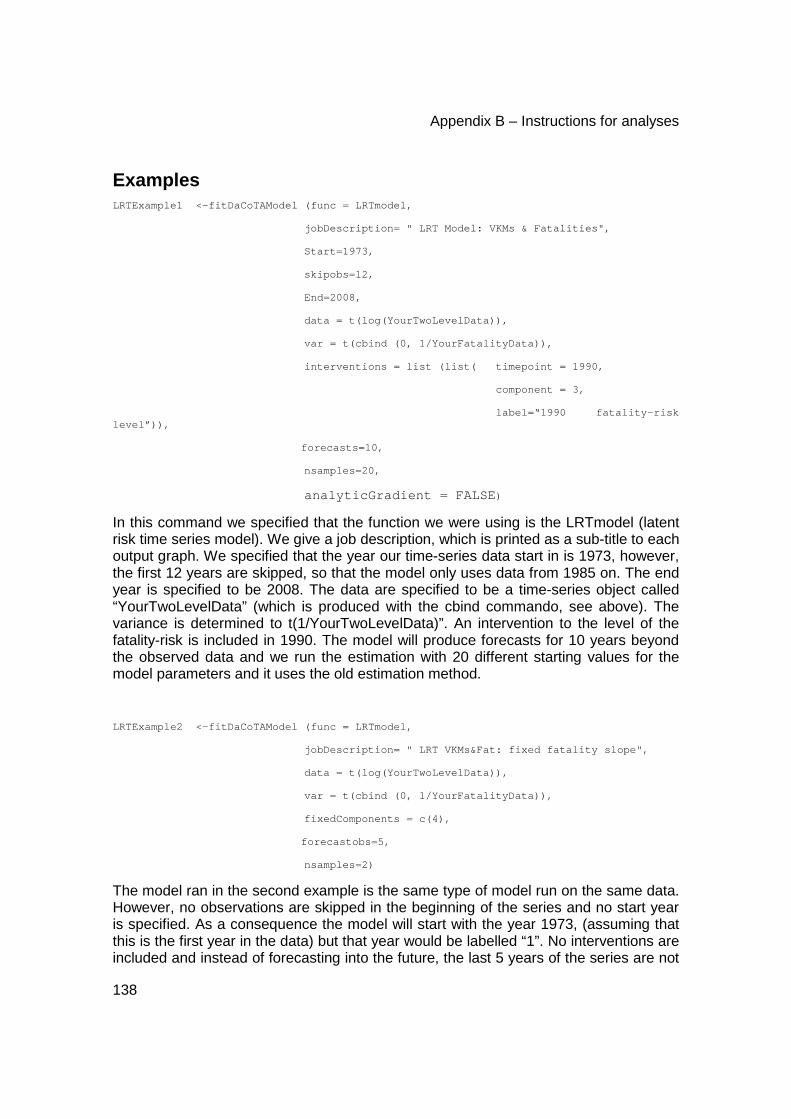
Appendix B – Instructions for analyses
138
Examples LRTExample1 <-fitDaCoTAModel (func = LRTmodel,
jobDescription= " LRT Model: VKMs & Fatalities",
Start=1973,
skipobs=12,
End=2008,
data = t(log(YourTwoL evelData)),
var = t(cbind (0, 1/Y ourFatalityData)),
interventions = list (list( timepoint = 1990,
component = 3,
label=“1990 fatality-risk level”)),
forecasts=10,
nsamples=20,
analyticGradient = FALSE )
In this command we specified that the function we were using is the LRTmodel (latent risk time series model). We give a job description, which is printed as a sub-title to each output graph. We specified that the year our time-series data start in is 1973, however, the first 12 years are skipped, so that the model only uses data from 1985 on. The end year is specified to be 2008. The data are specified to be a time-series object called “YourTwoLevelData” (which is produced with the cbind commando, see above). The variance is determined to t(1/YourTwoLevelData)”. An intervention to the level of the fatality-risk is included in 1990. The model will produce forecasts for 10 years beyond the observed data and we run the estimation with 20 different starting values for the model parameters and it uses the old estimation method.
LRTExample2 <-fitDaCoTAModel (func = LRTmodel,
jobDescription= " LRT VKMs&Fat: fixed fatality slope",
data = t(log(YourTwoL evelData)),
var = t(cbind (0, 1/Y ourFatalityData)),
fixedComponents = c(4),
forecastobs=5,
nsamples=2)
The model ran in the second example is the same type of model run on the same data. However, no observations are skipped in the beginning of the series and no start year is specified. As a consequence the model will start with the year 1973, (assuming that this is the first year in the data) but that year would be labelled “1”. No interventions are included and instead of forecasting into the future, the last 5 years of the series are not

D4.2: Forecasting traffic fatalities in European countries
139
included into the model. Those 5 years are forecasted on the basis of the other available data points. In the output, for those last 5 years the actual values and the forecasted ones (+ upper and lower limit) can be compared (forecastobs=5). Moreover the estimation is quick & dirty, with only 2 startingpoints (nsamples=2) and it uses the analytic gradient estimation method (which is the default).
Other options in fitDaCoTAModel There are a number of other options. Unfortunately, we are not able here to explain them. You could look them up in the DaCoTAStateSpaceIncludes.R file to see what they do (or ask Frits).
varIsMatrix
variableNames
independentComponents
commonComponents (will be addressed later)
explanatoryVariablesForState (see DaCoTA Manual for explanations)
BoxLjungLength
explanatoryVariablesWithError ((see DaCoTA Manual for explanations)
independentMeasurementError
partialDiffuseInitialState
nStrata (will be addressed as part of the advanced models)
independentStrata (will be addressed as part of the advanced models)
takeobs
Frequency
B.3.3 Output
DaCoTA.standardOutput The command DaCoTA.standardOutput (YourModelName)
gives you the complete output listed below under “text output” and additional graphical output, which we will not describe in detail here.
Fri Oct 22 12:01:50 2010 nsamples 10 previous maxim um new sample difference Fri Oct 22 12:02:17 2010 sample 1 -I nf 92.625899 Fri Oct 22 12:02:37 2010 sample 2 92.6258 99 92.624138 -1.761561e-03 Fri Oct 22 12:03:04 2010 sample 3 92.6258 99 92.628276 2.376792e-03 Fri Oct 22 12:03:25 2010 sample 4 92.6282 76 92.624827 -3.449351e-03 Fri Oct 22 12:03:43 2010 sample 5 92.6282 76 92.623306 -4.969817e-03

Appendix B – Instructions for analyses
140
Fri Oct 22 12:04:02 2010 sample 6 92.6282 76 92.598805 -2.947165e-02 Fri Oct 22 12:04:27 2010 sample 7 92.6282 76 92.624710 -3.566068e-03 Fri Oct 22 12:04:51 2010 sample 8 92.6282 76 92.624215 -4.061446e-03 Fri Oct 22 12:05:12 2010 sample 9 92.6282 76 92.623214 -5.061768e-03 Fri Oct 22 12:05:33 2010 sample 10 92.6282 76 92.606712 -2.156443e-02 Fri Oct 22 12:05:34 2010 Final maximum 92.628276
In the first lines the estimation procedure is described. This is an iterative process (i.e. in several cycles) in which the likelihood function is maximized. For each of the samples that you run (specified in nsamples, see Section 3.2.3.5) the estimated maximum is given. You can see that the differences are very small.
You might get a last line that looks somewhat like this
negative difference: t=16 dim=5 verschil=-1.164153e -10 = (1.000000e+06 - 1.000000e+06), Nt=-2.583834e-03, numerical roundoff error?
In that case please send this output to Frits + the code you were using and your Rdata file.
Model overview
Model name: Latent risk model Job description: BE Fat. & V KMs: LRT Model - 2 LEVELS (full) Model initial date: Fri Oct 15 09:18:06 2010 Model last date: Fri Oct 15 09:19:53 2010 DaCoTAStatespaceincludes version: dlm 0.5.3 1 3/10/2010 Data information Number of observations: 19 Number of dependent variables: 2 Forecastobs obs: 5 Series start: 1985 Series end: 2008 State space information Dimension of full state space: 4 Dimension of levels and trends: 4
The full state space can also contain explanatory variables and interventions. As long as there are none in the model, the levels and trends are equal to the full state space.
Model log likelihood: 75.5324 Akaike criterion: -150.117 Model number of parameters: 9
The number of parameters is important when you want to compare two models (nested into each other) with a likelihood-ratio test. The difference between the two likelihoods is chi-square distributed and the number of degrees of freedom is the difference between the number of parameters in one and in the other model.

D4.2: Forecasting traffic fatalities in European countries
141
Description of the state space structure
State space components nr Type Fixed Independent Shared Name 1 Level ................. Active Level exposure 2 Slope ................. Active slope exposure 3 Level ................. Active Level risk 4 Slope ................. Active slope risk
These are the numbers that you have to use in the R-code if you want to fix a component.
List of fixed components: 0 List of independent components: 0 Transition matrix T 1 1 0 0 0 1 0 0 0 0 1 1 0 0 0 1
See Commandeur & Koopman, (2007, p. 75).
Variances, covariances, & correlations of the state disturbances Transition covariance matrix Q 7.35984e-05 0 0.00021 7797 0 0 2.10835e-05 0 1.63664e-05 0.000217797 0 0.0029 8106 0 0 1.63664e-05 0 1.27806e-05
To read this and the following matrices, you might (mentally) write the name of the components listed above in the top row and in the left row. For each matrix structure, we will give an example of labelled tables in grey:
Level exp Slope exp Level risk Slope risk Level exp 7.35984e-05 0 0.000217797 0 Slope exp 0 2.10835e-05 0 1.63664e-05 Level ris 0.000217797 0 0.00298106 0 Slope risk 0 1.63664e-05 0 1.27806e-05
The first diagonal element of matrix Q are the variances of the state-disturbances. The off-diagonal elements are the covariances between the state-disturbances. The covariances between level and slope disturbances are structurally 0.
To see whether a particular component has a significant variance you have check whether the confidence interval given in the two tables below includes zero (in which case it is not significant). Note that in very rare cases, the confidence interval does not contain the actually estimated parameter. In that case the parameter is certainly not significant.

Appendix B – Instructions for analyses
142
Lower (2.50%) percentile of transition covariance m atrix Q samples 1.84841e-05 0 -0.00016 7447 0 0 7.44658e-06 0 -0.000500854 -0.000167447 0 0.0010 3359 0 0 -0.000500854 0 5.34066e-06 Upper (97.50%) percentile of transition covariance matrix Q samples 0.000239549 0 0.00074 8273 0 0 0.00105591 0 0.000282616 0.000748273 0 0.0064 3456 0 0 0.000282616 0 0.000976208
In the transition correlation matrix, you can see that for the Belgium example the trend disturbances for exposure are moderately correlated (.46) with those for the risk and the slope disturbances for the exposure are almost perfectly correlated with those for risk.
Transition correlation matrix 1 0 0.46 4977 0 0 1 0 0.997026 0.464977 0 1 0 0 0.997026 0 1
Relation between measurement & states Measurement matrix Z 1 0 0 0 1 0 1 0
The measurement matrix has a row for each observed variable and a column for each state component.
Level exp Slope exp Level risk Slope risk Exposure 1 0 0 0 Fatalities 1 0 1 0
In the measurement matrix, you can see that in an LRT model the observed exposure (first line) is equal to the trend of exposure (plus error) but the observed fatalities (second line) are the sum of the trend of exposure and the trend of the risk (plus error).
Variances, covariances, correlations of the observa tion errors
Measurement covariance matrix H (excluding additive time-varying component) 1.81409e-08 -2.10221e-09 -2.10221e-09 7.25754e-08
The measurement covariance matrix has for each observation error (one associated with exposure, the other associated with fatalities) one row and one column.
Obs.error exp Obs.error fat Observation error exp 1.81409e-08 -2. 10221e-09 Observation error fat -2.10221e-09 7. 25754e-08

D4.2: Forecasting traffic fatalities in European countries
143
This matrix gives you the variances and covariances of the error terms for the two measurement equations (exposure, fatalities). To test their significance you have to check whether the confidence interval given in the two tables below contains zero (in which case it is not significant).
Note that in very rare cases, the confidence interval does not contain the actually estimated parameter. In that case the parameter is certainly not significant.
Lower (2.50%) percentile of measurement matrix H sa mples 1.49428e-06 -0.000307753 -0.000307753 9.95679e-06 Upper (97.50%) percentile of measurement matrix H s amples 0.000193303 0.000289801 0.000289801 0.00422716
Measurement covariance matrix H (including additive time-varying component at time point 1985) 1.69333e-05 -2.10221e-09 -2.10221e-09 0.00055532 Measurement correlation matrix 1 -2.16787e-05 -2.16787e-05 1
Residual analysis
The residuals investigated in the following tests are the standardised one-step ahead prediction errors of the model . These have to be independently, identically, and normally distributed for statistical tests to hold.
Please take care interpreting the results! Box-Ljung tests Variable 1: Dependent varable 1 Variable 1: Dependent variable 1
Lag X-square df p value 3 0.998135 1 0.317762 4 3.35498 2 0.186843 5 3.50284 3 0.320394 Variable 2: Dependent variable 2 Lag X-square df p value 3 1.42185 1 0.2331 4 2.81153 2 0.245179 5 4.56623 3 0.206458

Appendix B – Instructions for analyses
144
The Box-Ljung test indicates for the first three lags that can be calculated (after correcting for the diffuse initial values of the level and the slope component) whether the Box-Ljung test is significant – first for exposure and then for the fatalities.
Heteroscedasticity tests Nr H df p value Label 1 2.69867 5 0.299881 Dependent variable 1 2 1.52609 5 0.654059 Dependent variable 2
The heteroscedasticity test, indicates whether the variance of the residuals is homogeneous across the time series.
Standardised Residual Normality tests Nr Skewness Kurtosis N p value Label 1 0.0570487 2.63998 0.101031 0.9 50739 Dependent variable 1 2 0.350818 2.91075 0.35435 0.83 7633 Dependent variable 2
The normality test indicates whether the residuals for either time series (exposure or fatalities) deviate from normality (which is not the case here).
Auxiliary Residual tests
The auxiliary residuals are standardised smoothed observation and state disturbances. The Output Auxiliary Residuals indicate the deviations of the observed data from the smoothed predictions. An extreme value in these residuals indicates an outlier observation. The state auxiliary residuals are based on the smoothed state disturbances divided by their variance. An extreme value in the level auxiliary residuals indicates a level break, i.e. a significant change in the level (a « jump » if you wish). An extreme value in the slope auxiliary residuals indicates a slope break, i.e., a significant change in the slope.
For a proper detection of outlier observations and level and slope breaks the only assumption that the auxiliary residuals have to satisfy is the assumption of normality.
Auxiliary Residual tests
Output Auxiliary Residual Normality tests Nr Skewness Kurtosis N p value Label 1 0.691262 2.96484 1.51415 0.469037 Dependent variable 1 2 -0.157537 2.11405 0.699981 0 .704695 Dependent variable 2 State Auxiliary Residual Normality tests Nr Skewness Kurtosis N p value Label 1 0.762558 3.0916 1.75078 0.4167 Level exposure 2 -0.448114 1.8701 1.55993 0.458422 slope exposure 3 -0.148959 2.1221 0.644596 0.724482 Level risk 4 -0.0444973 1.40547 1.80657 0.405237 slope risk

D4.2: Forecasting traffic fatalities in European countries
145
Post-sample predictions If you use the forecastobs option, R produces forecasts for the years specified. These post-sample predictions (including the criteria can also be obtained without producing the complete output by using the commando
DaCoTAPostSamplePredictions(YourModel)
Post-sample predictions Post-sample predictions for variable Dependent vari able 1 Obs. Observed Predicted Lower 95% Upper 95% 2004 11.4569 11.454 11.4 305 11.4776 2005 11.461 11.4664 11. 427 11.5057 2006 11.4765 11.4787 11.4 223 11.5352 2007 11.5008 11.491 11. 416 11.5661 2008 11.4904 11.5034 11.4 083 11.5985 Mean error: -0.00158673 Mean absolute error: 0.0066368 Mean squared error: 6.10054e-05 Mean percentage error: -0.0138382 Mean absolute percentage error: 0.0577875 Post-sample predictions for variable Dependent vari able 2 Obs. Observed Predicted Lower 95% Upper 95% 2004 7.0579 7.06485 6.93 275 7.19695 2005 6.99302 7.01977 6.83 201 7.20753 2006 6.97448 6.97468 6.73 701 7.21235 2007 6.97635 6.9296 6.64 384 7.21536 2008 6.85013 6.88452 6.55 093 7.2181 Mean error: -0.00431088 Mean absolute error: 0.0230102 Mean squared error: 0.000826435 Mean percentage error: -0.0631964 Mean absolute percentage error: 0.331235
Other output functions All output elements described above (and a few other like autocorrelation plots) can be obtained separately. The available output functions are listed below. We will not explain them here, as the names are more or less self-explanatory. All functions work if you type
NameOfDaCoTAOutputFunction (YourModelName)
but many of the functions also have options (like the alpha level). If you want to know more about them, you can look them up in the DaCoTAStateSpaceIncludes.R file.
DaCoTA.standardisedResidualplots DaCoTA.standardisedResidualQQplots

Appendix B – Instructions for analyses
146
DaCoTA.standardisedResidualACFplots DaCoTA.standardisedResidualPACFplots DaCoTA.outputAuxiliaryResidualplots DaCoTA.outputAuxiliaryResidualQQplots DaCoTA.stateAuxiliaryResidualplots DaCoTA.stateAuxiliaryResidualQQplots DaCoTA.PostSampleCUSUMplots (Post-sample cumulative residual sum) DaCoTA.oneaheadplots DaCoTA.forecastplots DaCoTA.smoothedplots DaCoTA.smoothedstateplots DaCoTA.stateforecastplots DaCoTA.likelihoodvalues DaCoTA.sampleTestsH DaCoTA.sampleTestsQ DaCoTA.PostSamplePredictions
DaCoTA.PrintstateResNormalityTests DaCoTA.PrintoutputResNormalityTests DaCoTA.PrintStdResNormalityTests DaCoTA.exportForecasts DaCoTA.forecastplots
Related Documents


