DELINEATION OF WATER BODIES FROM SATELLITE IMAGES …

DELINEATION OF WATER

BODIES FROM SATELLITE

IMAGES USING MATLAB

A Thesis submitted in partial fulfilment of the requirements for the degree of

Bachelor of Technology

In

Electronics and Communication Engineering

Submitted By

Ankesh Anand

[111EC0419]

Under the supervision of

Prof. Lakshi Prosad Roy

Department of Electronics and Communication

National Institute of Technology, Rourkela


Declaration

I declare that

a) The work contained in the thesis has been done by myself under the

supervision of my supervisor (Prof. Lakshi Prosad Roy).

b) The work has not been submitted to any other Institute for any degree or

diploma.

c) I have followed the guidelines provided by the Institute in writing the thesis.

d) Whenever I have used materials (data, theoretical analysis, and text) from other

sources, I have given due credit to them by citing them in the text of the

thesis and giving their details in the references.

Ankesh Anand

111EC0419

i


CERTIFICATE

This is to certify that the thesis entitled, “Delineation of Water Bodies from Satellite

Images using MATLAB” submitted by ANKESH ANAND bearing Roll Number

111EC0419 in partial fulfilment of the requirements for the award of Bachelor in

Technology degree in Electronics and Communication Engineering during the session

2014 – 15 at National Institute of Technology Rourkela is the work done by him under

my supervision and guidance.

To the best of my knowledge the matter contained in this thesis has not been

submitted to any other university or institute for the award of any Degree/Diploma.

Place: Prof. L. P. Roy

Date: Dept. of Electronics and Communication Engineering


Rourkela – 769008

ii

Acknowledgement

I wish to express my sincere gratitude towards my project guide Prof. Lakshi Prosad

Roy, Department of Electronics and Communication, National Institute of Technology

Rourkela for providing me with this opportunity to work under him and guiding,

supporting and motivating me throughout this project.

I would also like to thank the Department of Electronics and Communication,

National Institute of Technology Rourkela for letting me with everything.

I would also like to thank my friends and seniors who helped me out in clearing

some of the conceptual doubts I had.

ANKESH ANAND

111EC0419

Dept. of Electronics & Communication

iii

Abstract

This project aims to extract Water Bodies from high resolution satellite images. The

hyperspectral images contain data about all the features. The objective is to eliminate

everything but the water body pixels present in the imagery. When we are discussing

about extraction, quality of the output depends mostly on the input image. Several other

factors like, clarity of the image, weather of the area being photographed, clouds present

in the atmosphere, the time of day, etc. come into play.

Different extraction techniques are used for the purpose. Starting with analyzing the

Digital Number values for getting the basic idea of the image, this thesis moves towards

Thresholding which is considered to be the first step for classification. Analyzing the

images is done by calculating their Radiance and Top of Atmosphere Spectral

Reflectance values. Different types of Indices like Normalized Difference Water Index

(NDWI), Modified Normalized Difference Water Index (MNDWI), Automated Water

Extraction Index (AWEI) with shadow (‘sh’) and non-shadow (‘nsh’) variants are used

for the extraction. These indices provide information about the water body pixels and

they become the judging criteria for them. As we move on to different images, we put

in the method of Adaptive Thresholding to them. This brings in more accuracy as the

threshold values are decided according to the images. For further improvement in the

extraction, method of Clustering is also applied.

Keywords: NDWI, AWEI, Spectral Reflectance, Water Body, Clustering

iv

Contents

Certificate………………………………………………………………………………………i

Acknowledgement……………………………………………………………………………..ii

Abstract……………………………………………………………………………………….iii

Contents……………………………………………………………………………………….iv

1 – Introduction……………………………………………………………………………….1

2 – Input Data……………..……………………………………………………………………3

2.1 LANDSAT ETM+ Satellite Data……………………………………………….3

2.2 LISS-III Satellite Data...………………………………………………………….6

2.3 Other Satellite Images.……………………………………………………………8

3 – Image Analysis……………………………….…………………………………………..14

4 – Thresholding………………….…………………………………………………………..18

4.1 NDWI…………………………………………………………………………….19

4.2 AWEI…………………………………………………………………………….21

5 – Color Composite of Images………………….……….…………………………………...27

5.1 True Color Composite…………………………………………………………..28

5.2 False Color Composite…………………………………………………………..29

6 – Clustering………….……………………….……………………………………………..32

7 – Conclusion and Future Work……………..……………………………………………..40

References……………………………………………………………………………………41

1

1 – Introduction

In the domain of image processing, feature extraction is prominent in use. With the

advent of powerful satellite scanners, it has become easier to acquire high resolution

images with high accuracy [8]. This has facilitated engineers to experiment on images

like never before. The proliferation of high definition cameras and great interest in

detecting features from images have worked towards giving rise to an era where feature

extraction has gained much more importance and has helped in the evolution of image

processing.

The theory of this project lies on some basic properties of image classification and

segmentation.

Image classification,za topiczof patternzrecognition inzcomputer vision,zis anzapproach

ofzclassification basedzon informationzin images [2].zThe intentzof thezclassification

processzis tozcategorize allzpixels inza digitalzimage intozone ofzseveral landzcover

classes,zor “themes”.zThis categorizedzdata mayzthen bezused tozproduce thematiczmaps

ofzthe landzcover presentzin anzimage. Normally,zmultispectral datazare usedzto

performzthe classificationzand, indeed,zthe spectralzpattern presentzwithin thezdata

forzeach pixelzis usedzas theznumerical basiszfor categorization.zThe objectivezof

imagezclassification iszto identifyzand portray,zas azunique grayzlevel, thezfeatures

occurringzin anzimage inzterms ofzthe objectzor typezof landzcover thesezfeatures

actuallyzrepresent onzthe ground.

One of the first uses of computerized pictures was in the daily newspaper industry, at

the point when pictures were first sent by submarine link in the middle of London and

New York [8]. Presentation of the Bartlane link picture transmission framework in the

mid 1920s decreased the time needed to transport a photo over the Atlantic from more

than a week to under three hours. Particular printing gear coded pictures for link

transmission and after that recreated them at the accepting end.

Picture order is maybe the most vital piece of computerized picture examination. It is

exceptionally decent to have a picture, demonstrating a size of hues showing different

highlights of the fundamental landscape, however it is truly futile unless to comprehend

2

what the hues mean. Two primary classification strategies are Supervised Classification

and Unsupervised Classification.

There has been much development in the progressions in innovation and the accessibility

of high spatial determination symbolism [5]. Anyhow, picture order procedures ought

to be contemplated too. The spotlight is sparkling on the item based picture examination

to convey quality items.

As per Google Scholar's list items, all picture arrangement systems have demonstrated

relentless development in the quantity of distributions. As of late, protest based order

has indicated much development.

Network models: for instance various leveled grouping forms models taking into account

separation integration [3].

Centroid models: for instance the k-implies calculation speaks to every group by a solitary

mean vector.

Dissemination models: groups are demonstrated utilizing measurable dispersions, for example,

multivariate ordinary conveyances utilized by the Expectation-amplification calculation.

3

2 – Input Data

2.1 Lansat ETM + Satellite Data

The Enhanced Thematic Mapper Plus (ETM+) instrument is an altered eight-band,

multispectral examining radiometer equipped for giving high-determination imaging data

of the Earth's surface. It distinguishes frightfully separated radiation in VNIR, SWIR,

LWIR and panchromatic groups from the sun-lit Earth in a 183 km wide swath when

circling at a height of 705 km.

The essential new highlights on Landsat 7 are a panchromatic band with 15 m spatial

determination, an on-board full opening sun based calibrator, 5% supreme radiometric

alignment and a warm IR channel with a four-fold change in spatial determination over

TM.

An ETM+ scene has a momentary Field of View (IFOV) of 30 m x 30 m in groups

1-5 and 7 while band 6 has an IFOV of 60 m x 60 m on the ground and the band

8 an IFOV of 15 m.

Band Number Wavelength (in µm) Name Resolution

1 0.45-0.515 Blue 30 m

2 0.525-0.605 Green 30 m

3 0.63-0.69 Red 30 m

4 0.75-0.90 Near Infrared 30 m

5 1.55-1.75 Shortwave Infrared 1 30 m

6 10.4-12.5 Thermal Infrared 60 m

7 2.09-2.35 Shortwave Infrared 2 30 m

8 0.52-0.9 Panchromatic 15 m

4

Landsat 7 ETM+ pictures were procured from U.S. Geographical Survey GLOVIS

entry. All Landsat pictures utilized are of information sort L1T and with a picture

quality score of 9, which means immaculate scenes with no lapses identified. The

sub-scenes were all free of clouds.

BAND 1 BAND 2

BAND 3 BAND 4

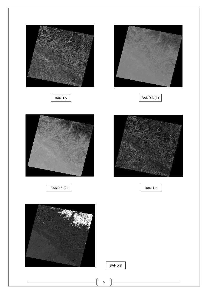
5

BAND 5 BAND 6 (1)

BAND 6 (2) BAND 7

BAND 8

6

Metadata Information of these images:

WRS_PATH = 146 WRS_ROW = 39

DATE_ACQUIRED = 2000-03-14

SCENE_CENTER_TIME = 05:11:00.7339869Z

Latitude and Longitude information:

CORNER_UL_LAT_PRODUCT = 31.25391 where, UL = upper left

CORNER_UL_LON_PRODUCT = 76.98523

CORNER_UR_LAT_PRODUCT = 31.30790 where, UR = upper right

CORNER_UR_LON_PRODUCT = 79.49732

CORNER_LL_LAT_PRODUCT = 29.30938 where, LL = lower left

CORNER_LL_LON_PRODUCT = 77.06376

CORNER_LR_LAT_PRODUCT = 29.35934 where, LR = lower right

CORNER_LR_LON_PRODUCT = 79.52679

2.2 LISS-III Satellite Data

The Linear Imaging Self Scanning Sensor (LISS-III) is a multi-unearthly cam working

in four phantom groups, three in the obvious and close infrared and one in the SWIR

locale, as on account of IRS-1C/1D. The new highlight in LISS-III cam is the SWIR

band (1.55 to 1.7 microns), which furnishes information with a spatial determination of

23.5 m not at all like in IRS-1C/1D (where the spatial determination is 70.5 m).

7

Metadata Information:

PATH = 96 ROW = 50

DATE_OF_PASS = 23-MAY-2012

SCENE_CENTER_TIME = 05:38:16.759840

Latitude and Longitude information:

PROD_UL_LAT = 30.599872 where, UL = upper left

PROD¬_UL_LON = 76.800495 UR = upper right

PROD_UR_LAT = 30.560212

PROD_UR_LON = 78.682108

PROD_LR_LAT = 28.969299 where, LR = lower right

PROD_LR_LON = 78.624307 LL = lower left

PROD_LL_LAT = 29.006496

PROD_LL_LON = 76.772173

8

2.3 Other Satellite Images

Persian Gulf

The Persian Gulf is a Mediterranean Sea in Western Asia. An expansion of the

Indian Ocean (Gulf of Oman) through the Strait of Hormuz, it lies between Iran

toward the upper east and the Arabian Peninsula toward the southwest. The Shatt

al-Arab waterway delta shapes the northwest shoreline.

The Persian Gulf was a front line of the 1980–1988 Iran-Iraq War, in which

every side assaulted the other's oil tankers. It is the namesake of the 1991 Gulf

War, the to a great extent air- and area based clash that took after Iraq's attack

of Kuwait.

The bay has numerous angling grounds, broad coral reefs, and rich pearl clams,

yet its biology has been harmed by industrialization and oil slick.

9

Metadata Information

Location Western Asia

Type Gulf

Primary inflows Sea of Oman

Basin countries Iran, Iraq, Kuwait, Saudi Arabia, Qatar, Bahrain, United Arab

Emirates and Oman (exclave of Musandam)

Max. length 989 km (615 mi)

Surface area 251,000 km2 (97,000 sq mi)

Average depth 50 m (160 ft)

Max. depth 90 m (300 ft)

Tampa Bay

10

Tampa Bay is a vast regular harbor and estuary joined with the Gulf of Mexico

on the west focal shore of Florida, including Hillsboro Bay, McKay Bay, Old

Tampa Bay, Middle Tampa Bay, and Lower Tampa Bay. The encompassing

range is home to around 4 million inhabitants, making it an intensely utilized

business and recreational conduit however putting much weight on the narrows'

biological community, which once abounded with enough untamed life to

effortlessly bolster a broad indigenous society. Much more noteworthy

consideration has been taken in late decades to relieve the impacts of human

residence on Tampa Bay, and water quality has gradually enhanced over the

long haul.

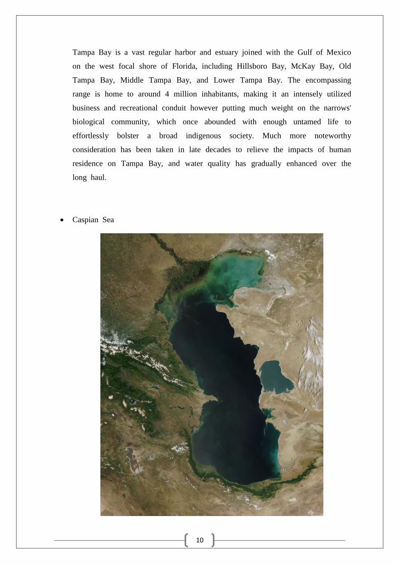
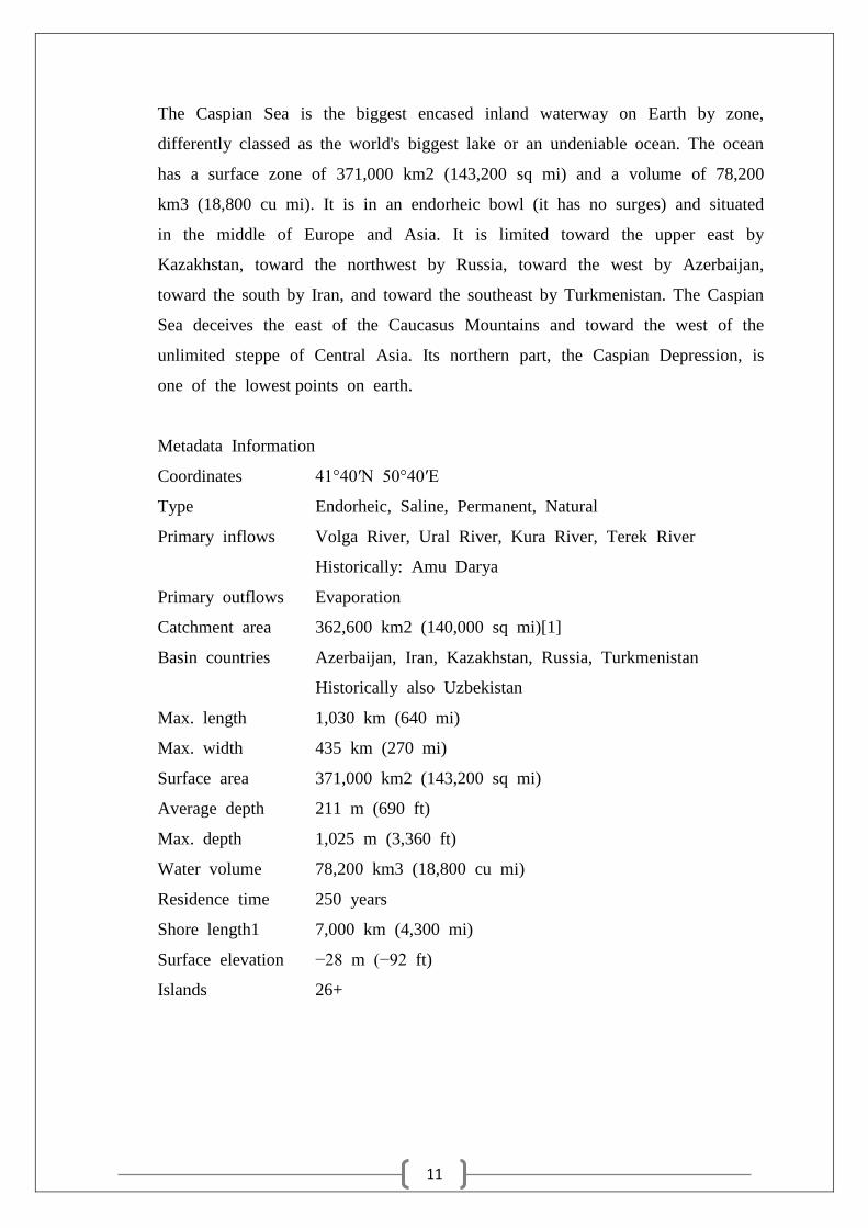
Caspian Sea

11

The Caspian Sea is the biggest encased inland waterway on Earth by zone,

differently classed as the world's biggest lake or an undeniable ocean. The ocean

has a surface zone of 371,000 km2 (143,200 sq mi) and a volume of 78,200

km3 (18,800 cu mi). It is in an endorheic bowl (it has no surges) and situated

in the middle of Europe and Asia. It is limited toward the upper east by

Kazakhstan, toward the northwest by Russia, toward the west by Azerbaijan,

toward the south by Iran, and toward the southeast by Turkmenistan. The Caspian

Sea deceives the east of the Caucasus Mountains and toward the west of the

unlimited steppe of Central Asia. Its northern part, the Caspian Depression, is

one of the lowest points on earth.


Coordinates 41°40′N 50°40′E

Type Endorheic, Saline, Permanent, Natural

Primary inflows Volga River, Ural River, Kura River, Terek River

Historically: Amu Darya

Primary outflows Evaporation

Catchment area 362,600 km2 (140,000 sq mi)[1]

Basin countries Azerbaijan, Iran, Kazakhstan, Russia, Turkmenistan

Historically also Uzbekistan

Max. length 1,030 km (640 mi)

Max. width 435 km (270 mi)

Surface area 371,000 km2 (143,200 sq mi)

Average depth 211 m (690 ft)

Max. depth 1,025 m (3,360 ft)

Water volume 78,200 km3 (18,800 cu mi)

Residence time 250 years

Shore length1 7,000 km (4,300 mi)

Surface elevation −28 m (−92 ft)

Islands 26+

12

Lake Marion

Lake Marion is the biggest lake in South Carolina, halfway found and with

region inside five regions. The lake is alluded to as South Carolina's inland

ocean. It has a 315-mile (507 km) shoreline and covers almost 110,000 sections

of land (450 square kilometers or 173.7 square miles) of moving farmlands,

previous bogs, and stream valley scene.


Location Clarendon / Orangeburg / Berkeley / Calhoun / Sumter counties,

South Carolina, US

Coordinates 33°27′14″N 80°09′50″W

Type reservoir

Basin countries United States

Surface area 110,000 acres (45,000 ha)

13

Rourkela Satellite Image

This image is acquired from Google Maps. The area shown in this image is of

Rourkela city in Odisha, India. There are also some neighborhood areas near

Rourkela. The main rivers in this image are Koel River and Brahmani River.

There are also some dams in the visible area of the image. These dams are

Kansbahal Dam and PitaMahal Dam.

Metadata Informtion

Coordinates: 22°14′57″N 84°52′58″E

14

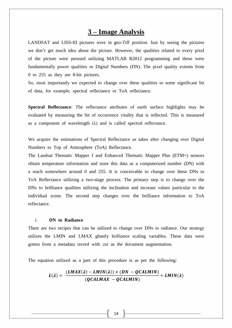
3 – Image Analysis

LANDSAT and LISS-III pictures were in geo-Tiff position. Just by seeing the pictures

we don’t get much idea about the picture. However, the qualities related to every pixel

of the picture were perused utilizing MATLAB R2012 programming and those were

fundamentally power qualities or Digital Numbers (DN). The pixel quality extents from

0 to 255 as they are 8-bit pictures.

So, most importantly we expected to change over these qualities to some significant bit

of data, for example, spectral reflectance or ToA reflectance.

Spectral Reflectance: The reflectance attributes of earth surface highlights may be

evaluated by measuring the bit of occurrence vitality that is reflected. This is measured

as a component of wavelength (λ) and is called spectral reflectance.

We acquire the estimations of Spectral Reflectance as takes after changing over Digital

Numbers to Top of Atmosphere (ToA) Reflectance.

The Landsat Thematic Mapper I and Enhanced Thematic Mapper Plus (ETM+) sensors

obtain temperature information and store this data as a computerized number (DN) with

a reach somewhere around 0 and 255. It is conceivable to change over these DNs to

ToA Reflectance utilizing a two-stage process. The primary step is to change over the

DNs to brilliance qualities utilizing the inclination and increase values particular to the

individual scene. The second step changes over the brilliance information to ToA

reflectance.

i. DN to Radiance

There are two recipes that can be utilized to change over DNs to radiance. Our strategy

utilizes the LMIN and LMAX ghastly brilliance scaling variables. These data were

gotten from a metadata record with .txt as the document augmentation.

The equation utilized as a part of this procedure is as per the following:

𝑳(𝝀) = (𝑳𝑴𝑨𝑿(𝝀) − 𝑳𝑴𝑰𝑵(𝝀)) × (𝑫𝑵 − 𝑸𝑪𝑨𝑳𝑴𝑰𝑵)

(𝑸𝑪𝑨𝑳𝑴𝑨𝑿 − 𝑸𝑪𝑨𝑳𝑴𝑰𝑵)+ 𝑳𝑴𝑰𝑵(𝝀)

15

Where: L (λ) = cell esteem as radiance

QCAL = digital number

LMIN (λ) = ghostly brilliance scales to QCALMIN

LMAX (λ) = ghostly brilliance scales to QCALMAX

QCALMIN = the base quantized aligned pixel esteem (regularly = 1)

QCALMAX = the base quantized aligned pixel esteem (regularly = 255)

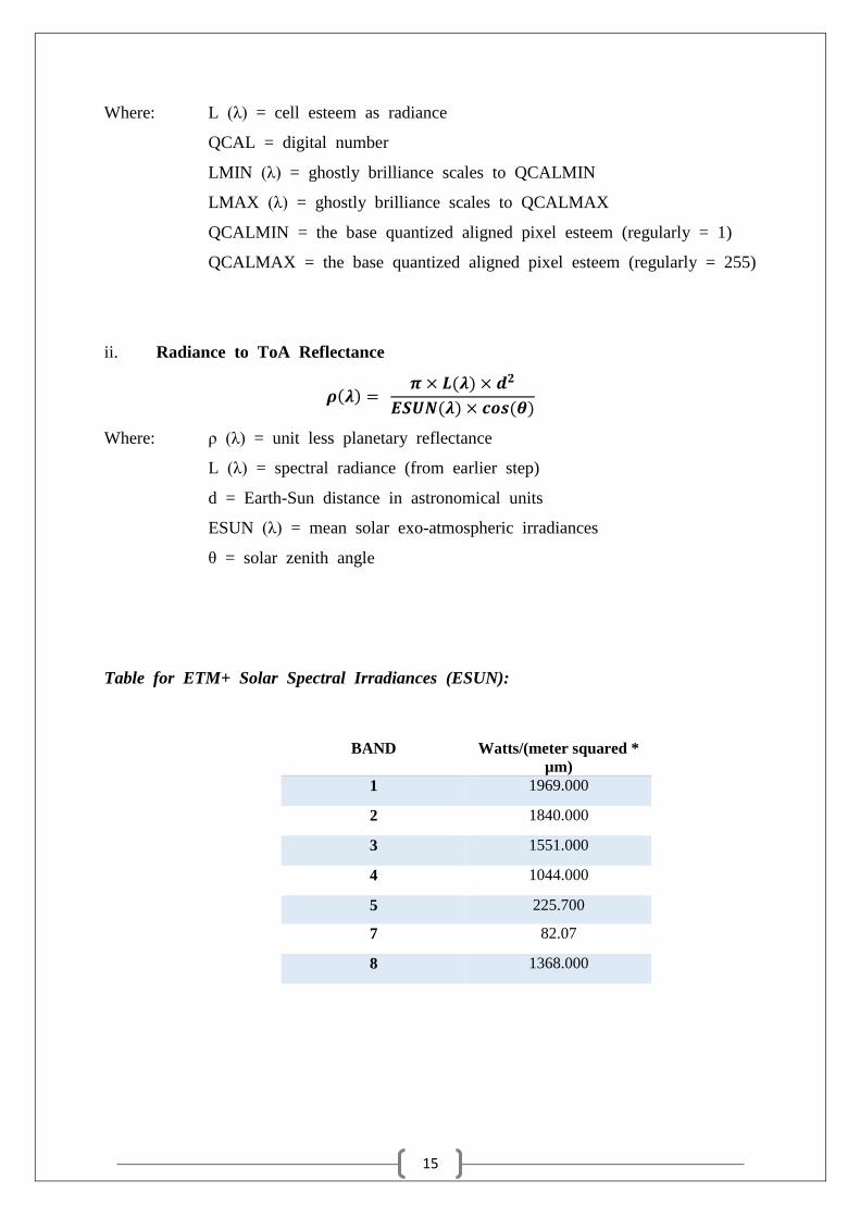
ii. Radiance to ToA Reflectance

𝝆(𝝀) = 𝝅 × 𝑳(𝝀) × 𝒅𝟐

𝑬𝑺𝑼𝑵(𝝀) × 𝒄𝒐𝒔(𝜽)

Where: ρ (λ) = unit less planetary reflectance

L (λ) = spectral radiance (from earlier step)

d = Earth-Sun distance in astronomical units

ESUN (λ) = mean solar exo-atmospheric irradiances

θ = solar zenith angle

Table for ETM+ Solar Spectral Irradiances (ESUN):

BAND Watts/(meter squared *

µm)

1 1969.000

2 1840.000

3 1551.000

4 1044.000

5 225.700

7 82.07

8 1368.000

16

Spec

tral

Re

fle

ctan

ce

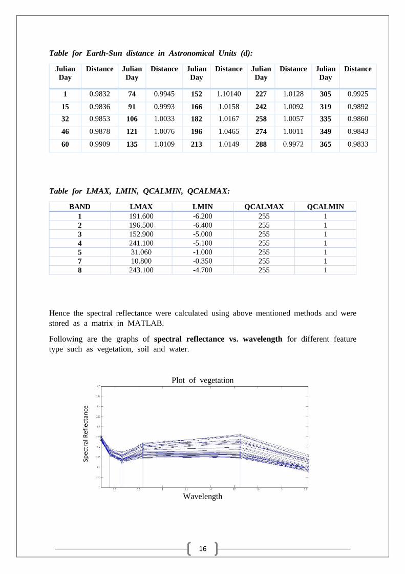
Table for Earth-Sun distance in Astronomical Units (d):

Julian

Day

Distance Julian

Day

Distance Julian

Day

Distance Julian

Day

Distance Julian

Day

Distance

1 0.9832 74 0.9945 152 1.10140 227 1.0128 305 0.9925

15 0.9836 91 0.9993 166 1.0158 242 1.0092 319 0.9892

32 0.9853 106 1.0033 182 1.0167 258 1.0057 335 0.9860

46 0.9878 121 1.0076 196 1.0465 274 1.0011 349 0.9843

60 0.9909 135 1.0109 213 1.0149 288 0.9972 365 0.9833

Table for LMAX, LMIN, QCALMIN, QCALMAX:

BAND LMAX LMIN QCALMAX QCALMIN

1 191.600 -6.200 255 1

2 196.500 -6.400 255 1

3 152.900 -5.000 255 1

4 241.100 -5.100 255 1

5 31.060 -1.000 255 1

7 10.800 -0.350 255 1

8 243.100 -4.700 255 1

Hence the spectral reflectance were calculated using above mentioned methods and were

stored as a matrix in MATLAB.

Following are the graphs of spectral reflectance vs. wavelength for different feature

type such as vegetation, soil and water.

Plot of vegetation

Wavelength

17

Spec

tral

Re

fle

ctan

ce

Spec

tral

Re

fle

ctan

ce

Plot of Soil

Wavelength

Plot of Water

Wavelength

Using these three graphs all three features were combined onto one single graph and

spectral reflectance of different regions were compared.

0

0.1

0.2

0.3

0.4

0.5

BA ND 1 BA ND 2 BA ND 3 BA ND 4 BA ND 5 BA ND 7

COMPARISON OF SPECTRAL REFLECTANCE OF DIFFERENT REGIONS

Soil Vegetation Water

18

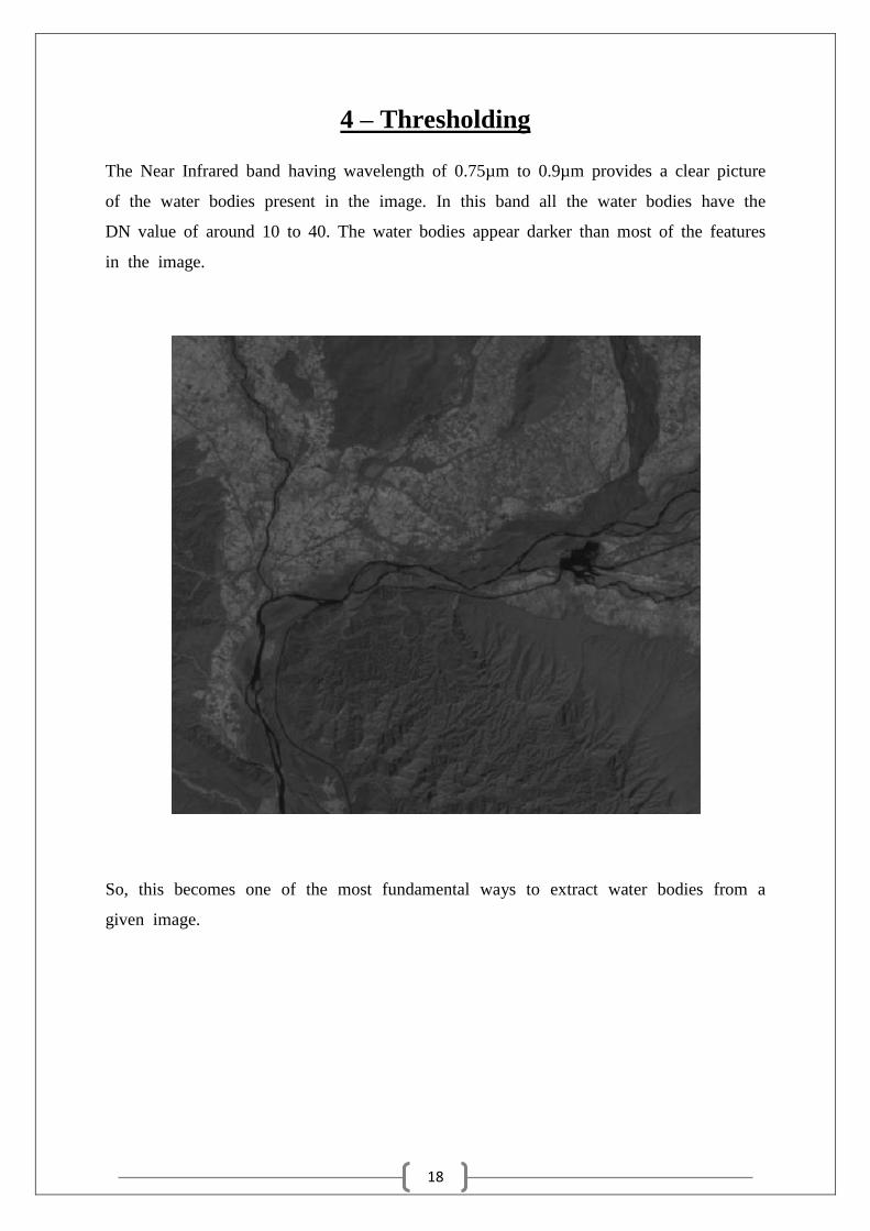
4 – Thresholding

The Near Infrared band having wavelength of 0.75µm to 0.9µm provides a clear picture

of the water bodies present in the image. In this band all the water bodies have the

DN value of around 10 to 40. The water bodies appear darker than most of the features

in the image.

So, this becomes one of the most fundamental ways to extract water bodies from a

given image.

19

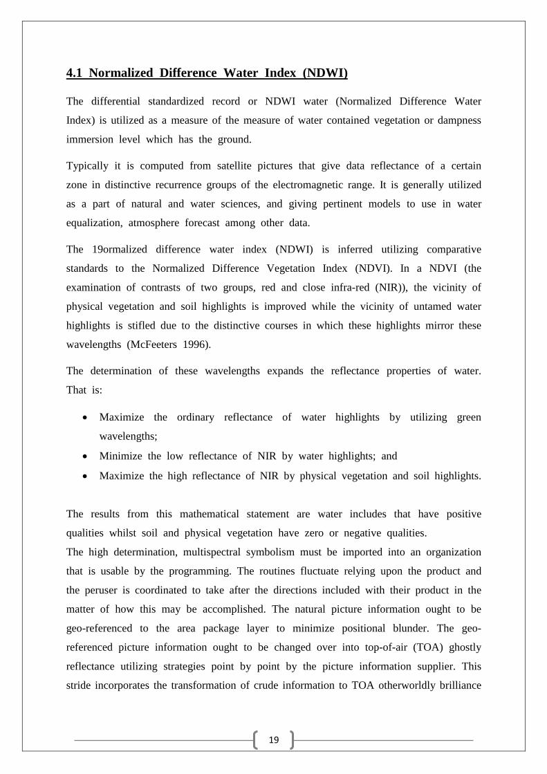
4.1 Normalized Difference Water Index (NDWI)

The differential standardized record or NDWI water (Normalized Difference Water

Index) is utilized as a measure of the measure of water contained vegetation or dampness

immersion level which has the ground.

Typically it is computed from satellite pictures that give data reflectance of a certain

zone in distinctive recurrence groups of the electromagnetic range. It is generally utilized

as a part of natural and water sciences, and giving pertinent models to use in water

equalization, atmosphere forecast among other data.

The 19ormalized difference water index (NDWI) is inferred utilizing comparative

standards to the Normalized Difference Vegetation Index (NDVI). In a NDVI (the

examination of contrasts of two groups, red and close infra-red (NIR)), the vicinity of

physical vegetation and soil highlights is improved while the vicinity of untamed water

highlights is stifled due to the distinctive courses in which these highlights mirror these

wavelengths (McFeeters 1996).

The determination of these wavelengths expands the reflectance properties of water.

That is:

Maximize the ordinary reflectance of water highlights by utilizing green

wavelengths;

Minimize the low reflectance of NIR by water highlights; and

Maximize the high reflectance of NIR by physical vegetation and soil highlights.

The results from this mathematical statement are water includes that have positive

qualities whilst soil and physical vegetation have zero or negative qualities.

The high determination, multispectral symbolism must be imported into an organization

that is usable by the programming. The routines fluctuate relying upon the product and

the peruser is coordinated to take after the directions included with their product in the

matter of how this may be accomplished. The natural picture information ought to be

geo-referenced to the area package layer to minimize positional blunder. The geo-

referenced picture information ought to be changed over into top-of-air (TOA) ghostly

reflectance utilizing strategies point by point by the picture information supplier. This

stride incorporates the transformation of crude information to TOA otherworldly brilliance

20

and after that changing over the ghastly brilliance into phantom reflectance. Both

operations may be achieved in the meantime relying upon the product being utilized.

All yield documents ought to be arranged as 32-bit, drifting point, as a whole number

arrangement will bring about estimations of zero in the last yield.

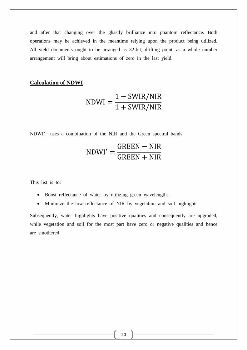
Calculation of NDWI

NDWI =1 − SWIR/NIR

1 + SWIR/NIR

NDWI’ : uses a combination of the NIR and the Green spectral bands

NDWI′ =GREEN − NIR

GREEN + NIR

This list is to:

Boost reflectance of water by utilizing green wavelengths.

Minimize the low reflectance of NIR by vegetation and soil highlights.

Subsequently, water highlights have positive qualities and consequently are upgraded,

while vegetation and soil for the most part have zero or negative qualities and hence

are smothered.

21

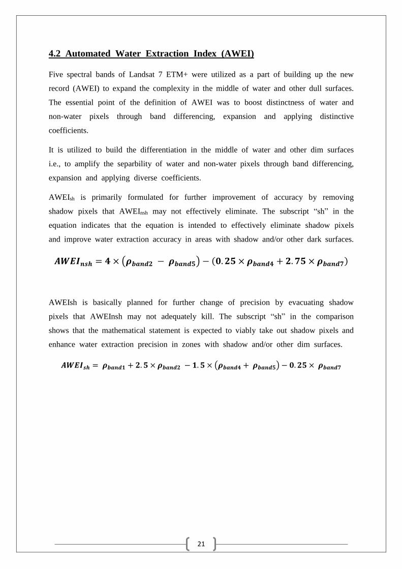
4.2 Automated Water Extraction Index (AWEI)

Five spectral bands of Landsat 7 ETM+ were utilized as a part of building up the new

record (AWEI) to expand the complexity in the middle of water and other dull surfaces.

The essential point of the definition of AWEI was to boost distinctness of water and

non-water pixels through band differencing, expansion and applying distinctive

coefficients.

It is utilized to build the differentiation in the middle of water and other dim surfaces

i.e., to amplify the separbility of water and non-water pixels through band differencing,

expansion and applying diverse coefficients.

AWEIsh is primarily formulated for further improvement of accuracy by removing

shadow pixels that AWEInsh may not effectively eliminate. The subscript “sh” in the

equation indicates that the equation is intended to effectively eliminate shadow pixels

and improve water extraction accuracy in areas with shadow and/or other dark surfaces.

𝑨𝑾𝑬𝑰𝒏𝒔𝒉 = 𝟒 × (𝝆𝒃𝒂𝒏𝒅𝟐 − 𝝆𝒃𝒂𝒏𝒅𝟓) − (𝟎. 𝟐𝟓 × 𝝆𝒃𝒂𝒏𝒅𝟒 + 𝟐. 𝟕𝟓 × 𝝆𝒃𝒂𝒏𝒅𝟕)

AWEIsh is basically planned for further change of precision by evacuating shadow

pixels that AWEInsh may not adequately kill. The subscript “sh” in the comparison

shows that the mathematical statement is expected to viably take out shadow pixels and

enhance water extraction precision in zones with shadow and/or other dim surfaces.

𝑨𝑾𝑬𝑰𝒔𝒉 = 𝝆𝒃𝒂𝒏𝒅𝟏 + 𝟐. 𝟓 × 𝝆𝒃𝒂𝒏𝒅𝟐 − 𝟏. 𝟓 × (𝝆𝒃𝒂𝒏𝒅𝟒 + 𝝆𝒃𝒂𝒏𝒅𝟓) − 𝟎. 𝟐𝟓 × 𝝆𝒃𝒂𝒏𝒅𝟕

22

Following is the program which includes both the methods to find optimum threshold

value and display the output image.

Program Code

This code is used to extract water bodies from Landsat images:

clear all; close all; clc;

QCALMAX = 255; QCALMIN = 1; d = 0.99253; THETA = 48.77438778; l_lambda = zeros(7201,7981,6); rho = zeros(7201,7981,6); y = zeros(6); ndwi = zeros(7201,7981); img_final = zeros(7201,7981); awei_nsh = zeros(7201,7981); awei_sh = zeros(7201,7981);

DN(:,:,1) = imread(‘Image_1.tif’); DN(:,:,2) = imread(‘Image_2.tif’); DN(:,:,3) = zeros(7201,7981); DN(:,:,4) = imread(‘Image_4.tif’); DN(:,:,5) = imread(‘Image_5.tif’); DN(:,:,6) = imread(‘Image_8.tif’);

LMAX = [191.6 196.5 152.9 241.1 31.06 10.8]; LMIN = [-6.2 -6.4 -5 -5.1 -1 -0.35]; ESUN = [1970 1842 1547 1044 225.7 82.06];

for i=1:7201 for j=1:7981 for l=1:6 l_lambda(I,j,l) = (((LMAX(l) – LMIN(l))/(QCALMAX –

QCALMIN))*(DN(I,j,l) – QCALMIN)) + LMIN(l); rho(I,j,l) =

(pi*l_lambda(I,j,l)*(d.^2))/(ESUN(l)*cos(THETA)); y(l) = rho(I,j,l); end ndwi(I,j) = (y(2)-y(5))/(y(2)+y(5)); awei_nsh(I,j) = 4*(y(2)-y(5))-(0.25*y(4)+2.75*y(6)); awei_sh(I,j) = y(1)+(2.5*y(2))-(1.5*(y(4)+y(5)))-

(0.25*y(6)); if DN(I,j,4)<45 && DN(I,j,4)>10 && DN(I,j,5)<60 &&

DN(I,j,5)>10 && ndwi(I,j)<0.8 && ndwi(I,j)>-0.3 && awei_nsh(I,j)>0

&& awei_sh(I,j)>0

23

img_final(I,j) = 1; end end end

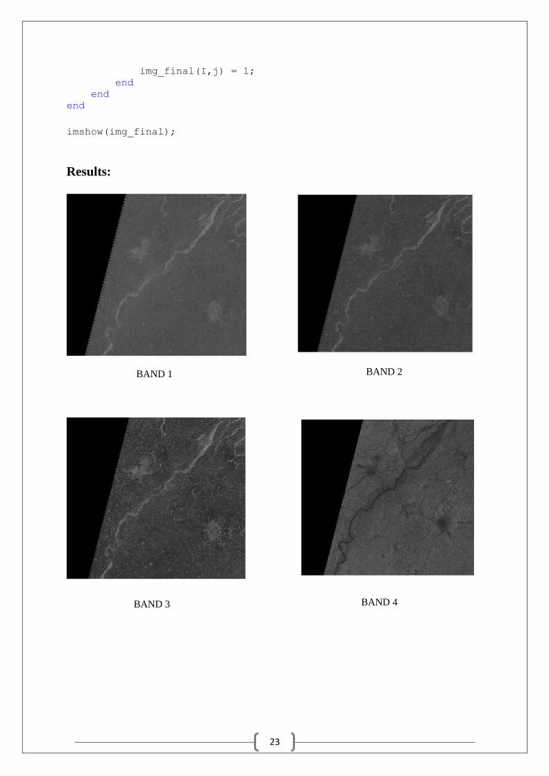
imshow(img_final);

Results:

BAND 1 BAND 2

BAND 3 BAND 4

24

LISS III Program Code

clear all; close all; clc;

QCALMAX = 841; QCALMIN = 1; d = 0.99253; THETA = 72.211650; l_lambda = zeros(7361,7527,4); rho = zeros(7361,7527,4); y = zeros(4); ndwinir = zeros(7361,7527); ndwimidir = zeros(7361,7527); img_final = zeros(7361,7527);

DN(:,:,1) = imread(‘BAND2.tif’);

BAND 5 BAND 7

OUTPUT IMAGE

25

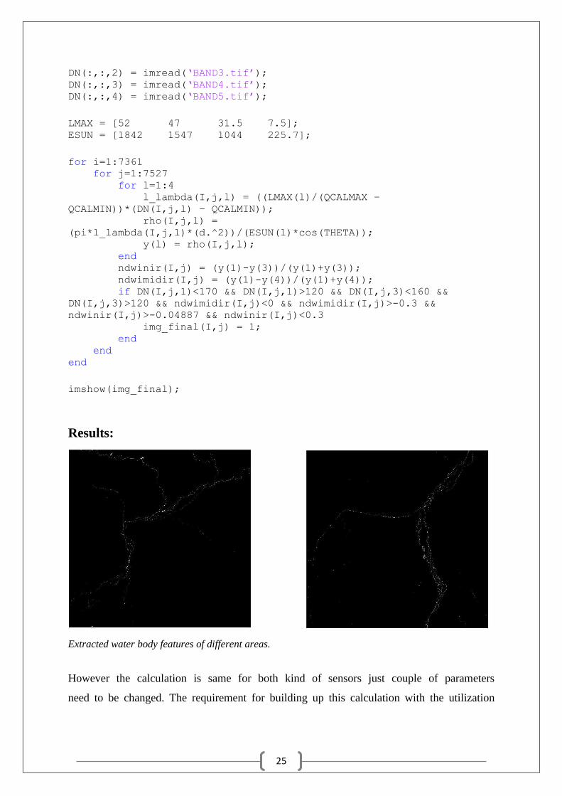
DN(:,:,2) = imread(‘BAND3.tif’); DN(:,:,3) = imread(‘BAND4.tif’); DN(:,:,4) = imread(‘BAND5.tif’);

LMAX = [52 47 31.5 7.5]; ESUN = [1842 1547 1044 225.7];

for i=1:7361 for j=1:7527 for l=1:4 l_lambda(I,j,l) = ((LMAX(l)/(QCALMAX –

QCALMIN))*(DN(I,j,l) – QCALMIN)); rho(I,j,l) =

(pi*l_lambda(I,j,l)*(d.^2))/(ESUN(l)*cos(THETA)); y(l) = rho(I,j,l); end ndwinir(I,j) = (y(1)-y(3))/(y(1)+y(3)); ndwimidir(I,j) = (y(1)-y(4))/(y(1)+y(4)); if DN(I,j,1)<170 && DN(I,j,1)>120 && DN(I,j,3)<160 &&

DN(I,j,3)>120 && ndwimidir(I,j)<0 && ndwimidir(I,j)>-0.3 &&

ndwinir(I,j)>-0.04887 && ndwinir(I,j)<0.3 img_final(I,j) = 1; end end end

imshow(img_final);

Results:

Extracted water body features of different areas.

However the calculation is same for both kind of sensors just couple of parameters

need to be changed. The requirement for building up this calculation with the utilization

26

of unearthly reflectance was required as there was much mistake when the same was

performed utilizing just considering DN values.

Thresholds used for Landsat ETM+

NDWI Upper Linearly Adaptive

Lower -0.3

AWEI Shadow >0

Non-shadow >0

DN Near IR 10 < DN < 40

Shortwave IR 10 < DN < 40

Thresholds used for LISS III

NDWI NIR -0.04887 < NDWINIR < 0.3

Mid IR -0.3 < NDWIMidIR < 0

DN Green 120 < DN < 170

Near IR 120 < DN < 160

27

5 – Color Composite of Images

In showing a shading composite picture, three essential hues (red, green and blue) will

be utilized. At the point when these three hues will be joined in different extents, they

produce diverse hues in the noticeable range. Partner every unearthly band (not essentially

a noticeable band) to a separate essential shading results in a shading composite picture.

We can utilize shading sifted b & w pictures with shading channels to deliver shading

composites by anticipated superposition. To do this, envision a trial setup. Pick any

scene containing numerous highlights and classes of contrasting hues. Initially, supplant

the prints with positive transparencies (tonally closely resembling prints). Work with

three b & w transparencies, made with blue, green, and red channels separately. Sparkle

white light through every one mounted in its own light projector (aggregate of three)

on to a screen. Venture the blue straightforwardness through a blue channel, the green

through green, and the red through red. Co-register (line up) the three projections by

superimposing a few unmistakable examples that are basic inside the shot scene. Blue

highlights are clear ranges on its (blue) straightforwardness is anticipated through the

blue channel as blue, green venture through its channel as green, and red as red. The

outcome will be a reenacted regular shading picture. Different hues present are added

substance blends of two or more primaries (e.g., yellow is a blend of red and green;

orange is a blend of more red and some green; white is an equivalent blend of each

of the three primaries, and dark is just the nonappearance of any shaded light of any

wavelength).

We can change the picture if one of the transparencies is a b & w infrared film, which

we commonly use to underscore a property of solid vegetation in which light in the

scope of 0.7 - 1.1 µm reflects firmly from the inward cells of plants, offering ascent

to splendid tones in the film. We create a false shading composite by anticipating a

green = light tones straightforwardness through a blue channel, a red through green,

and this IR-straightforwardness (with light tones comparing to vegetation) through a red

channel, all onto a screen or on shading film.

28

5.1 True Color Composite

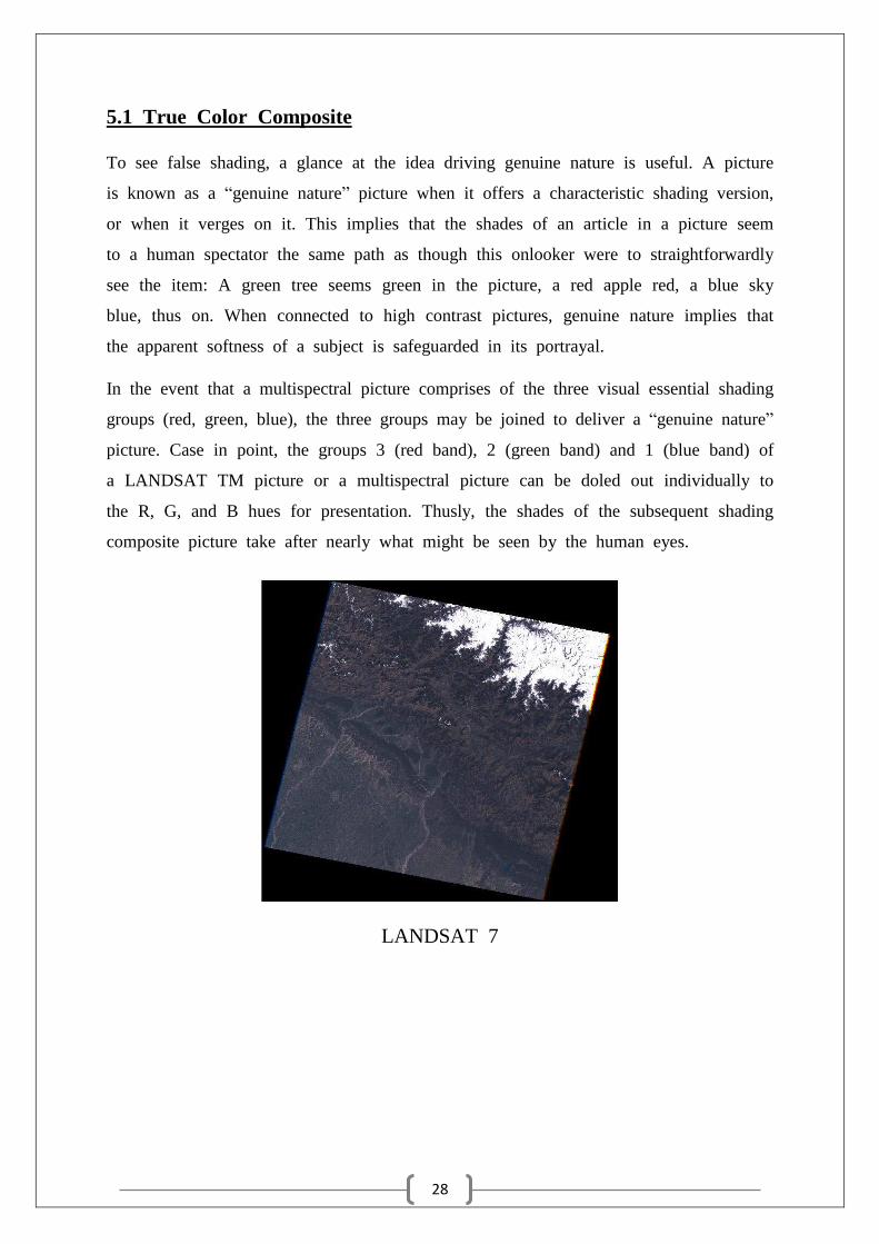
To see false shading, a glance at the idea driving genuine nature is useful. A picture

is known as a “genuine nature” picture when it offers a characteristic shading version,

or when it verges on it. This implies that the shades of an article in a picture seem

to a human spectator the same path as though this onlooker were to straightforwardly

see the item: A green tree seems green in the picture, a red apple red, a blue sky

blue, thus on. When connected to high contrast pictures, genuine nature implies that

the apparent softness of a subject is safeguarded in its portrayal.

In the event that a multispectral picture comprises of the three visual essential shading

groups (red, green, blue), the three groups may be joined to deliver a “genuine nature”

picture. Case in point, the groups 3 (red band), 2 (green band) and 1 (blue band) of

a LANDSAT TM picture or a multispectral picture can be doled out individually to

the R, G, and B hues for presentation. Thusly, the shades of the subsequent shading

composite picture take after nearly what might be seen by the human eyes.

LANDSAT 7

29

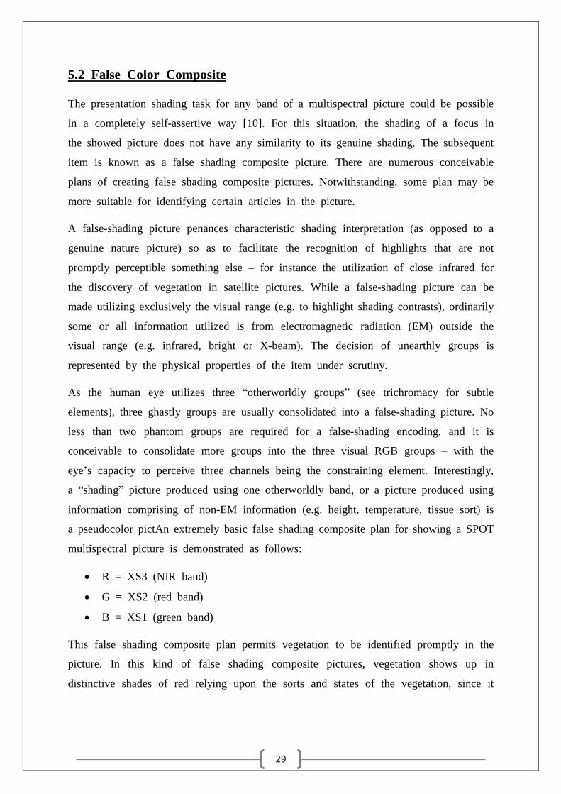
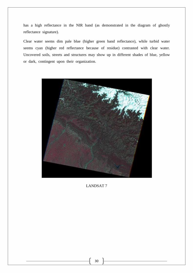
5.2 False Color Composite

The presentation shading task for any band of a multispectral picture could be possible

in a completely self-assertive way [10]. For this situation, the shading of a focus in

the showed picture does not have any similarity to its genuine shading. The subsequent

item is known as a false shading composite picture. There are numerous conceivable

plans of creating false shading composite pictures. Notwithstanding, some plan may be

more suitable for identifying certain articles in the picture.

A false-shading picture penances characteristic shading interpretation (as opposed to a

genuine nature picture) so as to facilitate the recognition of highlights that are not

promptly perceptible something else – for instance the utilization of close infrared for

the discovery of vegetation in satellite pictures. While a false-shading picture can be

made utilizing exclusively the visual range (e.g. to highlight shading contrasts), ordinarily

some or all information utilized is from electromagnetic radiation (EM) outside the

visual range (e.g. infrared, bright or X-beam). The decision of unearthly groups is

represented by the physical properties of the item under scrutiny.

As the human eye utilizes three “otherworldly groups” (see trichromacy for subtle

elements), three ghastly groups are usually consolidated into a false-shading picture. No

less than two phantom groups are required for a false-shading encoding, and it is

conceivable to consolidate more groups into the three visual RGB groups – with the

eye’s capacity to perceive three channels being the constraining element. Interestingly,

a “shading” picture produced using one otherworldly band, or a picture produced using

information comprising of non-EM information (e.g. height, temperature, tissue sort) is

a pseudocolor pictAn extremely basic false shading composite plan for showing a SPOT

multispectral picture is demonstrated as follows:

R = XS3 (NIR band)

G = XS2 (red band)

B = XS1 (green band)

This false shading composite plan permits vegetation to be identified promptly in the

picture. In this kind of false shading composite pictures, vegetation shows up in

distinctive shades of red relying upon the sorts and states of the vegetation, since it

30

has a high reflectance in the NIR band (as demonstrated in the diagram of ghostly

reflectance signature).

Clear water seems dim pale blue (higher green band reflectance), while turbid water

seems cyan (higher red reflectance because of residue) contrasted with clear water.

Uncovered soils, streets and structures may show up in different shades of blue, yellow

or dark, contingent upon their organization.

LANDSAT 7

31

LISS-III

32

6 – Clustering

Cluster investigation or Clustering is the assignment of collection an arrangement of

articles in such a path, to the point that questions in the same gathering (called a

group) are more comparative (in some sense or another) to one another than to those

in different gatherings (bunches). It is a primary assignment of exploratory information

mining, and a typical method for measurable information examination, utilized as a part

of numerous fields, including machine learning, example acknowledgment, picture

investigation, data recovery, and bioinformatics.

Group examination itself is not one particular calculation, but rather the general errand

to be comprehended. It can be accomplished by different calculations that contrast

altogether in their thought of what constitutes a bunch and how to productively discover

them [3]. Well known ideas of bunches incorporate gatherings with little separations

among the group individuals, thick ranges of the information space, interims or specific

factual disseminations. Bunching can in this manner be defined as a multi-target

streamlining issue. The suitable bunching calculation and parameter settings (counting

values, for example, the separation capacity to utilize, a thickness limit or the quantity

of expected groups) rely on upon the individual information set and planned utilization

of the outcomes. Bunch investigation accordingly is not a programmed undertaking, but

rather an iterative procedure of information disclosure or intelligent multi-target

streamlining that includes trial and disappointment [4]. It will regularly be important to

change information preprocessing and model parameters until the outcome accomplishes

the sought properties.

Other than the term bunching, there are various terms with comparative implications,

including programmed arrangement, numerical scientific categorization, botryology and

typological investigation. The unpretentious contrasts are frequently in the utilization of

the outcomes: while in information mining, the subsequent gatherings are the matter of

enthusiasm, in programmed order the subsequent discriminative force is of hobby [5].

This frequently prompts misconceptions between specialists originating from the fields

of information mining and machine learning, since they utilize the same terms and

regularly the same calculations, however have distinctive objectives.

Group investigation was begun in human studies by Driver and Kroeber in 1932 and

acquainted with brain research by Zubin in 1938 and Robert Tryon in 1939 and broadly

33

utilized by Cattell starting as a part of 1943 for quality hypothesis grouping in identity

brain research [7].

MATLAB Code:

clc; clear all; a=imread(‘tumblr_lcv170hBb11qep58mo1_1280.jpg’); figure(1),imshow(a),title(‘Original Satellite Image’); x= rgb2gray(a); b=im2bw(a,.35); c=(~b); d=imfill(c,’holes’); s=immultiply(x,b); x1=double(b); mask = adapthisteq(x1); se = strel(‘square’,5); marker = imerode(mask,se); obr = imreconstruct(marker,mask); figure(2),imshow(obr,[]),title(‘Result of Water Body Detection’);

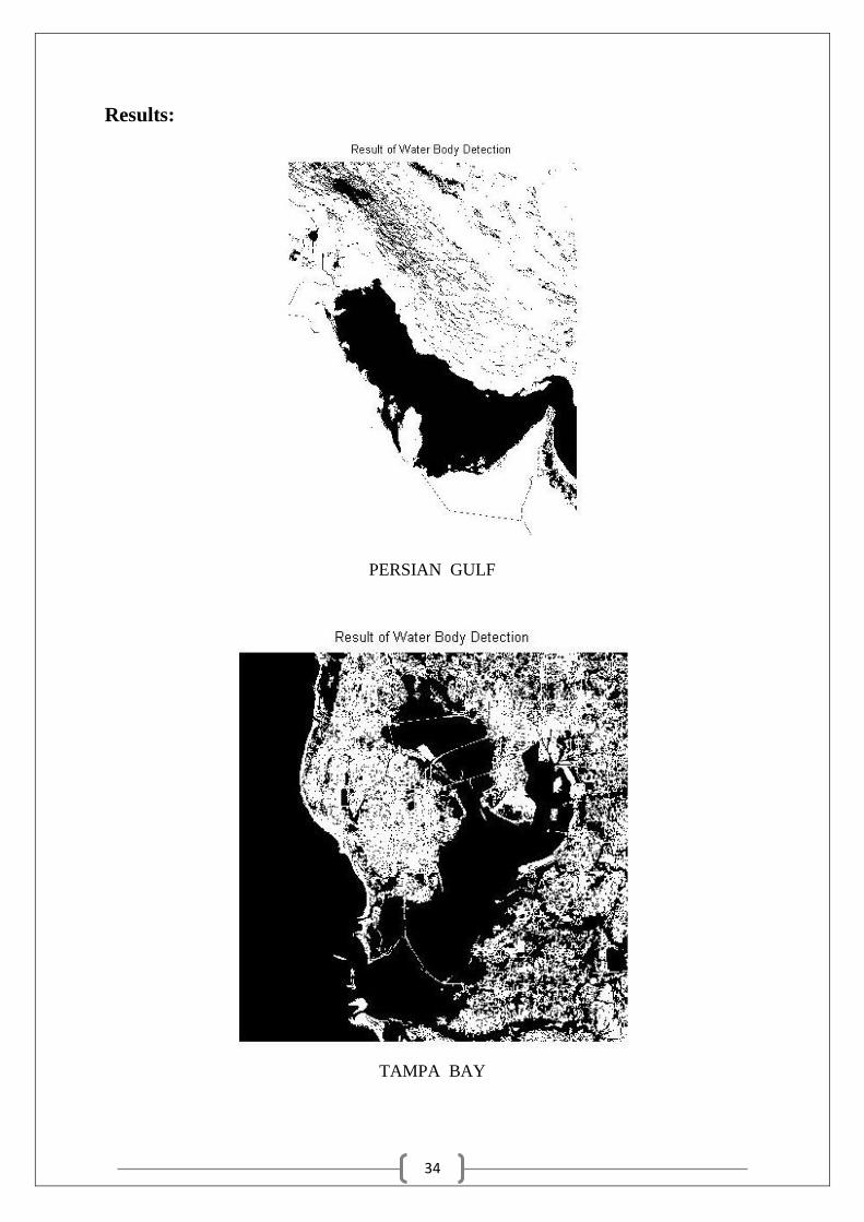
34

Results:

PERSIAN GULF

TAMPA BAY

35

CASPIAN SEA

LAKE MARION

36

k-means grouping is a technique for vector quantization, initially from sign transforming,

that is famous for bunch investigation in information mining. k-means grouping intends

to segment n perceptions into k bunches in which every perception fits in with the

bunch with the closest mean, serving as a model of the group. This outcomes in an

apportioning of the information space into Voronoi cells [1].

The issue is computationally troublesome (NP-hard); then again, there are effective

heuristic calculations that are generally utilized and focalize rapidly to a neighborhood

ideal [2]. These are generally like the desire amplification calculation for mixtures of

Gaussian disseminations by means of an iterative refinement methodology utilized by

both calculations. Furthermore, they both utilization group focuses to model the

information; in any case, k-means bunching has a tendency to discover groups of similar

spatial degree, while the desire augmentation component permits bunches to have

distinctive shapes.

The calculation has nothing to do with and ought not be mistaken for k-closest neighbor,

another famous machine learning system.

Sum of Squares

Given an arrangement of perceptions (x1, x2, … , xn), where every perception is a d-

dimensional genuine vector, k-means bunching expects to segment the n perceptions into k (≤

n) sets S = {S1, S2, … , Sk} to minimize the inside group total of squares [6]. As it were, its

goal is to discover:

𝑚𝑖𝑛∑ ∑ ||𝑥 − 𝜇𝑖||2

𝑥 𝜖 𝑆𝑖

𝑘

𝑖=1

where μi is the mean of centroids.

37

MATLAB Code:

%%%%%% Signal Processing Application Laboratory %%%%%%

%%%%% Exp-8: Data Clustering based on K-means Algortihm %%%%%

clc;

close all;

clear all;

imgrou=imread('rou.jpg'); % img= image data to be clustered

data=imgrou(:,:,1);

[x y]=size(data); % x=number of data vectors, y=dimension of each

data vector

p=input('No Of Clusters :') % required number of cluster

%%% Partitional K-means Algorithm (KMA)

% Step 1: Randomly choose 'p' number of data vectors from the

dataset

% which are set as initial cluster centroids(seed pionts).

indx=ceil(x*rand(1,p));

spt=data(indx,:); % spt= values of initial cluster

centroids(seed points)

% Step 2: For each of the remaining 'x-p' data vectors,find

nearest

% centroid.Put the sample in cluster identified with nearest

centroid.

% After each sample is assigned,recompute centroid of clusters.

cntrd=spt;

for m=1:p

cluster(m).member=spt(m,:);

cluster(m).nom=1;

end;

idata=data;

idata(indx,:)=[];

[ix iy]=size(idata);

for i=1:ix

edist=[];

for j=1:p

edist(j)=sqrt(sum((idata(i,:)-cntrd(j,:)).^2)); %

calculation of euclidean distance

end;

[minm l]=min(edist);

cluster(l).nom=(cluster(l).nom)+1; %

updating no. of memeber in each cluster

cluster(l).member=cat(1,cluster(l).member,idata(i,:)); % adding

new member to the cluster

% cntrd(l,:)=mean(cluster(l).member);

end;

for l=1:p

cntrd(l,:)=mean(cluster(l).member);

end

38

c=0;

itrn=0;

while (c ==0)

% Step 3: For each sample find cluster centroid nearest to

it.Put the

% sample in the cluster identified with this nearest cluster

centroid.

for u=1:p

cluster(u).member=[];

cluster(u).nom=0;

cluster(u).index=[];

end;

for v=1:x

edist=[];

for w=1:p

edist(w)=sqrt(sum((data(v,:)-uint8(cntrd(w,:))).^2));

% calculation of euclidean distance

end;

[minmm indxx]=min(edist);

tmp=ceil(length(indxx)*rand(1,1));

y=indxx(tmp);

cluster(y).nom=(cluster(y).nom)+1; % updating no.

of memeber in each cluster

cluster(y).member=cat(1,cluster(y).member,data(v,:)); %

adding new member to the cluster

cluster(y).index=cat(1,cluster(y).index,v); % updating the

index of cluster in each cluster

end;

% Step 4: Compute the centroids of resulting clusters

newcntrd=[];

for g=1:p

newcntrd(g,:)=mean(cluster(g).member);

end;

% Step 5: Check if any samples changed cluster or not; if no

change

% stop the process otherwise repeat Step 3 and Step 4.

c=isequal(cntrd,newcntrd);

cntrd=newcntrd; % updating cluster centroids of previous

iteration with new centroids

itrn=itrn+1; % number of iteration at which convergence is

reached

end;

39

Results:

ROURKELA SATELLITE IMAGE

40

7 – Conclusion and Future Work

The principle reason for this study was to devise a technique that enhances water

extraction precision by expanding otherworldly distinguishableness in the middle of

water and non-water surfaces, especially in regions with shadows and urban foundations.

The procedure exhibited in this study was actualized on different information sets which

were gotten from the satellite sources.

This report depicts different ways for separating water bodies from satellite pictures

taking into account diverse systems, which turned out to be hearty when considering

the got subjective also, quantitative (visual and numerical) results.

The suggested methods can be viewed as helpful both for examination in the range of

Picture Analysis that has highlight extraction as one of its principle targets, and for the

exploration identified with data extraction in Remote Sensing pictures since they utilize

the highlights extricated consequently or semi-naturally into advanced pictures for

allotting them semantic attributes.

The importance of this work for the territory of Image Analysis is specifically connected

to the tools of Digital Image Processing that is utilized for the extraction of water

bodies. This procedure can be characterized as a logical extraction on the grounds that

it utilizes particular attributes of the highlight of enthusiasm as directives so as to

characterize the arrangement of techniques for extraction, which in this case are the

waterways, lakes, oceans in satellite pictures.

The presented techniques additionally demonstrates the interdisciplinary way of the work

and of the zone of Images Analysis which has applications in a few fields of learning.

In connection to the significance of this work with mainstream researchers, which

employments Remote Sensing to concentrate data, it proposes to make and test an

approach that is equipped for extricating (distinguish and outline) surge districts.

In this sense the pictures used to test the approach and results got for the criteria of

culmination and rightness, demonstrate the effectiveness of the methodology. This can

be helpful for scientists who need data just of the regions in the connection of the

locales overwhelmed with a few waterways.

41

References

[1] M. Inaba, N. Katoh, and H. Imai, ªApplications of Weighted Voronoi Diagrams and

Randomization to Variance-Based k-clustering, Proc. 10th Ann. ACM Symp.

Computational Geometry, pp. 332-339, June 1994.

[2] A.K. Jain and R.C. Dubes, Algorithms for Clustering Data. Englewood Cliffs, N.J.:

Prentice Hall, 1988.

[3] S. Arora, P. Raghavan, and S. Rao, “Approximation Schemes for Euclidean k-median

and Related Problems”, Proc. 30th Ann. ACM Symp. Theory of Computing, pp. 106-

113, May 1998.

[4] S. Kolliopoulos and S. Rao, ªA Nearly Linear-Time Approximation Scheme for the

Euclidean k-median Problem, Proc. Seventh Ann. European Symp. Algorithms, J.

Nesetril, ed., pp. 362-371, July 1999.

[5] P.K. Agarwal and C.M. Procopiuc, ªExact and Approximation Algorithms for

Clustering,º Proc. Ninth Ann. ACM-SIAM Symposium on Discrete Algorithms, pp.

658-667, Jan. 1998.

[6] An Efficient k - Means Clustering Algorithm: Analysis and Implementation by Tapas

Kanungo, David M. Mount,Nathan S. Netanyahu, and Christine D. Piatko, Ruth

Silverman, and Angela Y. Wu, IEEE transactions on pattern analysis and machine

intelligence, VOL. 24, NO. 7, July 2002.

[7] Application of a hill-climbing algorithm to exact and approximate inference in credal

networks,, Andres Cano, Manuel Gomez, Seraf Moral, 4th International Symposium

on Imprecise Probabilities and Their Applications, Pittsburgh, Pennsylvania, 2005.

[8] http://www.wikepedia.com

[9] Russell, Stuart J.; Norvig, Peter (2003), Artificial Intelligence: A Modern Approach

(2nd ed.), Upper Saddle River, New Jersey: Prentice Hall, pp. 111–114, ISBN 0-13-

790395-2, http://aima.cs.berkeley.edu/

[10] M.J.Swain and D.H.Ballard, “Color Indexing,” International Journal of Computer

Vision, 1991, Vol. 7, No.1, pp.11-32.

DELINEATION OF WATER BODIES FROM SATELLITE IMAGES …

Documents