Delaunay Triangulation as a New Coverage Measurement

Sensors 2011, 11, 3163-3176; doi:10.3390/s110303163OPEN ACCESS

sensorsISSN 1424-8220

www.mdpi.com/journal/sensors

Article

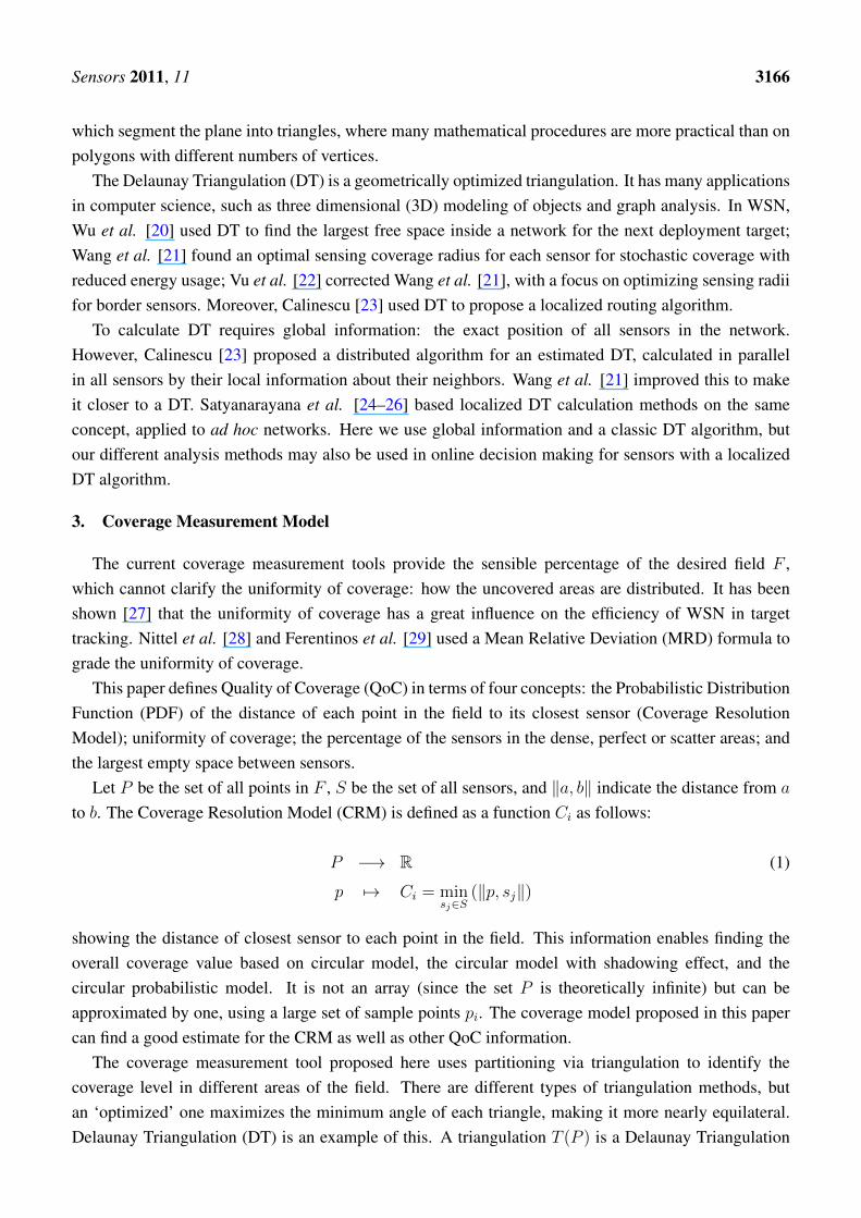
Delaunay Triangulation as a New Coverage MeasurementMethod in Wireless Sensor NetworkHassan Chizari 1, Majid Hosseini 1, Timothy Poston 2, Shukor Abd Razak 1 andAbdul Hanan Abdullah 1,?

1 Faculty of Computer Science and Information Systems, Universiti Teknologi Malaysia, Malaysia;E-Mails: [email protected] (H.C.); [email protected] (M.H.); [email protected] (S.A.R.)

2 Chief Scientist, Nordic River Software AB, Umea, Sweden; E-Mail: [email protected]

? Author to whom correspondence should be addressed; E-Mail: [email protected].

Received: 15 January 2011; in revised form: 25 February 2011 / Accepted: 28 February 2011 /Published: 15 March 2011

Abstract: Sensing and communication coverage are among the most important trade-offsin Wireless Sensor Network (WSN) design. A minimum bound of sensing coverageis vital in scheduling, target tracking and redeployment phases, as well as providingcommunication coverage. Some methods measure the coverage as a percentage value, butdetailed information has been missing. Two scenarios with equal coverage percentage maynot have the same Quality of Coverage (QoC). In this paper, we propose a new coveragemeasurement method using Delaunay Triangulation (DT). This can provide the value for allcoverage measurement tools. Moreover, it categorizes sensors as ‘fat’, ‘healthy’ or ‘thin’to show the dense, optimal and scattered areas. It can also yield the largest empty areaof sensors in the field. Simulation results show that the proposed DT method can achieveaccurate coverage information, and provides many tools to compare QoC between differentscenarios.

Keywords: wireless sensor network; sensing coverage; communication coverage; quality ofcoverage; delaunay triangulation

Sensors 2011, 11 3164

1. Introduction

Wireless Sensor Networks (WSNs) have attracted attention in much research on ad hoc networks. Themany challenges in successful WSN implementation include sensor scheduling, routing, re-deploymentand sensor movement. Since the WSN goal is to sense a phenomenon, in each challenge a fit tool tomeasure sensing coverage is important to success.

Sensing coverage is defined [1] as the ratio of the sensible area to the entire desired area. While in theideal environment these areas must be equal (Deterministic Coverage), Zhang et al. [2] showed that thesacrifice of a small amount of coverage (Stochastic Coverage) can increase network lifetime by 3 to 7times. A gain in network lifetime is very important in WSN, where it is usually impractical to change orcharge the sensors’ batteries, and very costly to deploy new sensors on the field. Stochastic coverage iswidely accepted by researchers and WSN application designers. Like sensing coverage, communicationcoverage is a deterministic factor which needs all the active sensors to be able to communicate with oneanother. An important issue in any WSN is to check whether the communication coverage is completeamong active sensors.

A WSN mission is usually started by deploying a large number of sensors. A scheduling algorithmdefines different sets of sensors, which must each achieve a lower bound coverage value set in the missiongoal. When one set of sensors is activated, the rest are turned off and wait for their time triggers tobe activated. A scheduling algorithm can increase the lifetime of a WSN by reserving the energy inredundant sensors.

One class of scheduling algorithm needs global information about sensors and their positions, whileothers just work with local information gathered by each sensor about its neighbors. Either way, a goodscheduling algorithm that covers the whole network can prolong the network lifetime. However, differentmethods to measure sensing coverage may give various results, which makes comparison hard. The termof Quality of Coverage (QoC) has not been defined clearly enough to provide a judgment tool betweendifferent coverage algorithms.

In this paper, we propose a new method to determine sensing/communication coverage, whichprovides more detailed QoC information than its predecessors about the uniformity of coverage, whichhas remarkable influence on network efficiency. This technique, based on Delaunay Triangulation (DT),is useful in many different challenges of WSN.

Organizationally, Section 2 discusses the research background, prior methods for calculating sensingcoverage, and some previous research in WSN that used DT. Section 3 introduces the proposed coveragemeasurement tool. Section 4 provides four methods for analyzing the DT results. The paper concludeswith Section 5.

2. Research Background

There are several ways to define coverage in WSNs, each with advantages and disadvantages. Thissection discusses existing calculation methods, and presents other known applications of DT in WSN.

Sensors 2011, 11 3165

2.1. Coverage Calculation Methods

The simplest measure of sensing coverage [3,4] divides the mission field into a grid of small squares,each representing one sensible area that should contain at least one sensor: the exact location of sensorsinside the squares is ignored. The sensing coverage is the percentage of squares with at least one activesensor inside.

The favorite definition of sensing and communication coverage is the circular model [2,5–8]. In thismodel, the sensors have a sensing radius Rs, whose value could be a constant like Rs = 20m [5], orrelated to transmission range (Rt) by Rs >= Rt/

√3 [2] or Rs = Rt/2 [8].

The circular model with shadowing [1,9,10] is similar, but has an additional radius Ru for a regionoutside of the guaranteed sensing area, which is still sensible with some probability p > 0. Accordingly,the sensing coverage integrates over all target locations the probability:

• If the object is in Rs range, it will be sensed with probability 1;

• If the object is between Rs and Ru, it will be sensed with probability p;

• If the object is out of Ru range, it is not sensed.

Another way to quantify sensing coverage is circular probabilistic model [11–13], which is like thecircular model with shadowing effect when Rs = 0. It integrates:

• If the object is in the Ru range, it will be sensed with probability p;

• The value of p decreases with distance from the sensor.

• If the object is out of the Ru range, it is not sensed.

Soreanu et al. [14] give a non-unit-circular model for measuring the sensing coverage, with anelliptical sensing area that the sensors can widen or narrow by using different power levels. Theseadjustments can significantly improve the network coverage.

Voronoi decomposition [15–18] partitions the points of field into convex ‘area of influence’ polygonsaround their nearest sensors. All previous work has used this as a clustering system to determine sensorscheduling: coverage was still quantified using the circular model.

To the best of our knowledge, the probabilistic circular and non-unit-circular models, like Voronoidecomposition, are used to determine whether or not a phenomenon can be detected, rather than toquantify the overall coverage of a sensor network. Only the grid-based and the circular models are theonly methods so far that are employed to determine how much of the desired area is sensible.

2.2. Delaunay Triangulation in WSNs

To quantify the Quality of Coverage (QoC) in the empty spaces between sensors requires a spatialsegmentation algorithm whose characteristics reveal the QoC information. Among the choices are theVoronoi algorithm, the Gabriel graph [19] and triangulation methods. Voronoi creates a polygon aroundeach sensor. The Gabriel graph is a subgraph of the Delaunay triangulation edge graph, so its edgesdivide the plane into larger polygons. A triangulation algorithm creates a graph of edges between sensors,

Sensors 2011, 11 3166

which segment the plane into triangles, where many mathematical procedures are more practical than onpolygons with different numbers of vertices.

The Delaunay Triangulation (DT) is a geometrically optimized triangulation. It has many applicationsin computer science, such as three dimensional (3D) modeling of objects and graph analysis. In WSN,Wu et al. [20] used DT to find the largest free space inside a network for the next deployment target;Wang et al. [21] found an optimal sensing coverage radius for each sensor for stochastic coverage withreduced energy usage; Vu et al. [22] corrected Wang et al. [21], with a focus on optimizing sensing radiifor border sensors. Moreover, Calinescu [23] used DT to propose a localized routing algorithm.

To calculate DT requires global information: the exact position of all sensors in the network.However, Calinescu [23] proposed a distributed algorithm for an estimated DT, calculated in parallelin all sensors by their local information about their neighbors. Wang et al. [21] improved this to makeit closer to a DT. Satyanarayana et al. [24–26] based localized DT calculation methods on the sameconcept, applied to ad hoc networks. Here we use global information and a classic DT algorithm, butour different analysis methods may also be used in online decision making for sensors with a localizedDT algorithm.

3. Coverage Measurement Model

The current coverage measurement tools provide the sensible percentage of the desired field F ,which cannot clarify the uniformity of coverage: how the uncovered areas are distributed. It has beenshown [27] that the uniformity of coverage has a great influence on the efficiency of WSN in targettracking. Nittel et al. [28] and Ferentinos et al. [29] used a Mean Relative Deviation (MRD) formula tograde the uniformity of coverage.

This paper defines Quality of Coverage (QoC) in terms of four concepts: the Probabilistic DistributionFunction (PDF) of the distance of each point in the field to its closest sensor (Coverage ResolutionModel); uniformity of coverage; the percentage of the sensors in the dense, perfect or scatter areas; andthe largest empty space between sensors.

Let P be the set of all points in F , S be the set of all sensors, and ‖a, b‖ indicate the distance from a

to b. The Coverage Resolution Model (CRM) is defined as a function Ci as follows:

P −→ R (1)

p 7→ Ci = minsj∈S

(‖p, sj‖)

showing the distance of closest sensor to each point in the field. This information enables finding theoverall coverage value based on circular model, the circular model with shadowing effect, and thecircular probabilistic model. It is not an array (since the set P is theoretically infinite) but can beapproximated by one, using a large set of sample points pi. The coverage model proposed in this papercan find a good estimate for the CRM as well as other QoC information.

The coverage measurement tool proposed here uses partitioning via triangulation to identify thecoverage level in different areas of the field. There are different types of triangulation methods, butan ‘optimized’ one maximizes the minimum angle of each triangle, making it more nearly equilateral.Delaunay Triangulation (DT) is an example of this. A triangulation T (P ) is a Delaunay Triangulation

Sensors 2011, 11 3167

of P , denoted as DT (P ), if and only if the circumcircle of any triangle of T strictly contains no otherpoint of P . For more information about DT algorithms and application, see [30,31].

For a network with more than three sensors, DT is an optimal triangulation with the properties:

1. The outer polygon of the triangulation for a set of points is convex.

2. Each sensor is connected by triangle edges to its closest neighbors.

3. If no three sensors lie on one shared straight line, each has degree at least two.

4. The circumcircle of each triangle contains no other sensor.

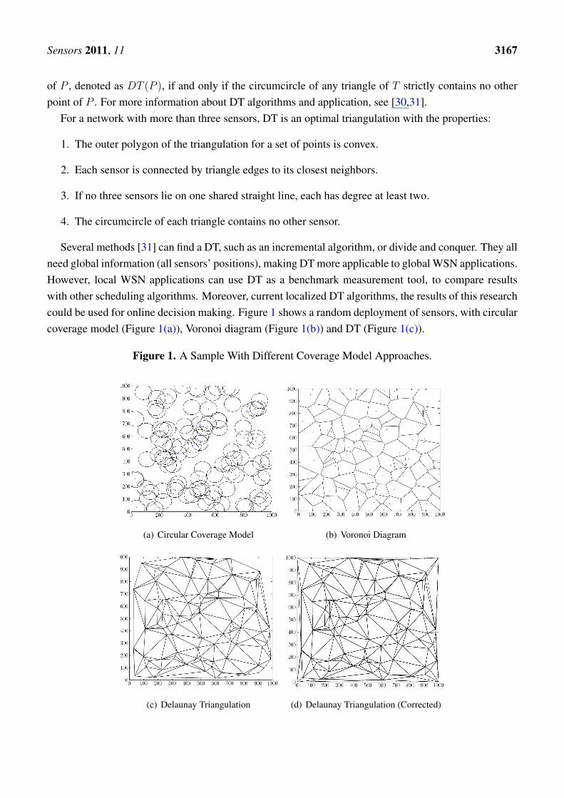
Several methods [31] can find a DT, such as an incremental algorithm, or divide and conquer. They allneed global information (all sensors’ positions), making DT more applicable to global WSN applications.However, local WSN applications can use DT as a benchmark measurement tool, to compare resultswith other scheduling algorithms. Moreover, current localized DT algorithms, the results of this researchcould be used for online decision making. Figure 1 shows a random deployment of sensors, with circularcoverage model (Figure 1(a)), Voronoi diagram (Figure 1(b)) and DT (Figure 1(c)).

Figure 1. A Sample With Different Coverage Model Approaches.

(a) Circular Coverage Model (b) Voronoi Diagram

(c) Delaunay Triangulation (d) Delaunay Triangulation (Corrected)

Sensors 2011, 11 3168

3.1. Modification in DT

To use the DT as a WSN coverage measurement tool, we add two rules before generating the DTgraph. The first rule adds extra sensors at the corners of the field, assumed convex (in our examples,a square), since as in Figure 1(c), the outer polygon of the coverage model may not cover all the field.Since the outer polygon in DT is always convex, additional sensors on the field corners lead to a fulltriangulation of the field as in Figure 1(d). Secondly, if three sensors cannot create a triangle becausethey are collinear, we move one of them by a random multiple of 0.5 m to let the DT create a triangle.

4. Analysis Methods

This paper proposes five QoC parameters to analyze the DT. The first step finds local and globalcommunication coverage of a network. The second divides sensors into three categories: in dense,scattered or perfect areas. The third extracts information from DT which easily shows the coveragevalues for circular model with and without shadowing effect and probability, as well as uniformity ofcoverage. The last finds the biggest empty area between sensors as a comparison parameter amongnetwork planning applications.

4.1. Network Coverage Analysis

The term ‘network coverage’ is used for both sensing and communication. Communication networkcoverage is the ability to send and receive packets to and from all the active sensors in the field. Wheneach sensor has at least one neighbor in its communication range, local communication coverage issatisfied. When a sensor can send information to all active sensors in the field, via other sensors, generalcommunication coverage is achieved. Both local and global communication coverage are very importantfor a WSN. Network Coverage Analysis (NCA) is a good tool to examine both.

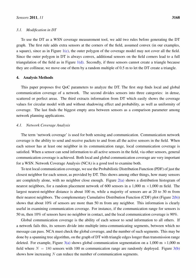
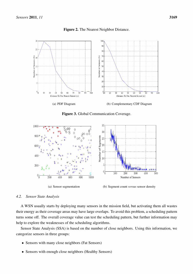
To test local communication coverage, we use the Probabilistic Distribution Function (PDF) of just theclosest neighbor for each sensor, as provided by DT. This shows among other things, how many sensorsare completely alone, with no neighbor close enough. Figure 2(a) shows a distribution histogram ofnearest neighbors, for a random placement network of 600 sensors in a 1,000 m ×1,000 m field. Thelargest nearest-neighbor distance is about 100 m, while a majority of sensors are at 20 to 30 m fromtheir nearest neighbors. The complementary Cumulative Distribution Function (CDF) plot (Figure 2(b))shows that about 10% of sensors are more than 50 m from any neighbor. This information is clearlyuseful in examining communication coverage. For instance, if the communication range for sensors is50 m, then 10% of sensors have no neighbor in contact, and the local communication coverage is 90%.

Global communication coverage is the ability of each sensor to send information to all others. Ifa network fails this, its sensors divide into multiple intra-communicating segments, between which nomessage can pass. NCA must check the global coverage, and the number of such segments. This may bedone by a spanning tree algorithm, on the graph of DT with triangle edges longer than transmission rangedeleted. For example, Figure 3(a) shows global communication segmentation on a 1,000 m ×1,000 mfield where N = 180 sensors with 100 m communication range are randomly deployed. Figure 3(b)shows how increasing N can reduce the number of communication segments.

Sensors 2011, 11 3169

Figure 2. The Nearest Neighbor Distance.

(a) PDF Diagram (b) Complementary CDF Diagram

Figure 3. Global Communication Coverage.

(a) Sensor segmentation (b) Segment count versus sensor density

4.2. Sensor State Analysis

A WSN usually starts by deploying many sensors in the mission field, but activating them all wastestheir energy as their coverage areas may have large overlaps. To avoid this problem, a scheduling patternturns some off. The overall coverage value can test the scheduling pattern, but further information mayhelp to explore the weaknesses of the scheduling algorithms.

Sensor State Analysis (SSA) is based on the number of close neighbors. Using this information, wecategorize sensors in three groups:

• Sensors with many close neighbors (Fat Sensors)

• Sensors with enough close neighbors (Healthy Sensors)

Sensors 2011, 11 3170

• Sensors with few close neighbors (Thin Sensors)

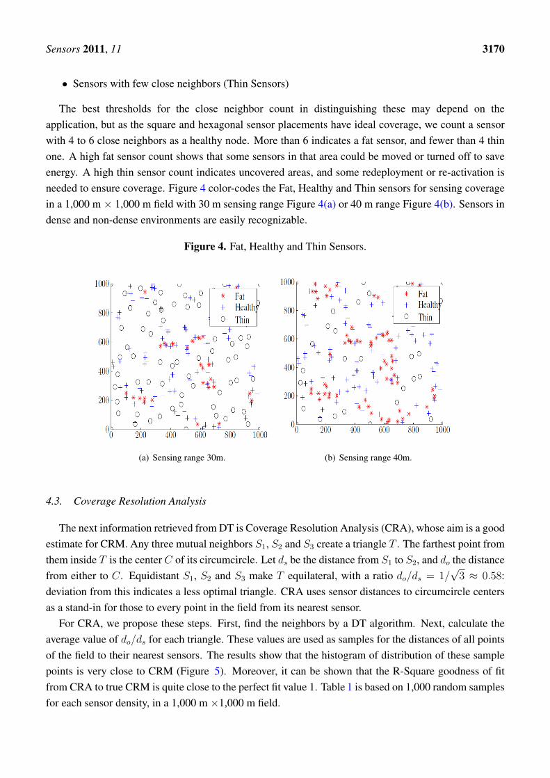
The best thresholds for the close neighbor count in distinguishing these may depend on theapplication, but as the square and hexagonal sensor placements have ideal coverage, we count a sensorwith 4 to 6 close neighbors as a healthy node. More than 6 indicates a fat sensor, and fewer than 4 thinone. A high fat sensor count shows that some sensors in that area could be moved or turned off to saveenergy. A high thin sensor count indicates uncovered areas, and some redeployment or re-activation isneeded to ensure coverage. Figure 4 color-codes the Fat, Healthy and Thin sensors for sensing coveragein a 1,000 m × 1,000 m field with 30 m sensing range Figure 4(a) or 40 m range Figure 4(b). Sensors indense and non-dense environments are easily recognizable.

Figure 4. Fat, Healthy and Thin Sensors.

(a) Sensing range 30m. (b) Sensing range 40m.

4.3. Coverage Resolution Analysis

The next information retrieved from DT is Coverage Resolution Analysis (CRA), whose aim is a goodestimate for CRM. Any three mutual neighbors S1, S2 and S3 create a triangle T . The farthest point fromthem inside T is the center C of its circumcircle. Let ds be the distance from S1 to S2, and do the distancefrom either to C. Equidistant S1, S2 and S3 make T equilateral, with a ratio do/ds = 1/

√3 ≈ 0.58:

deviation from this indicates a less optimal triangle. CRA uses sensor distances to circumcircle centersas a stand-in for those to every point in the field from its nearest sensor.

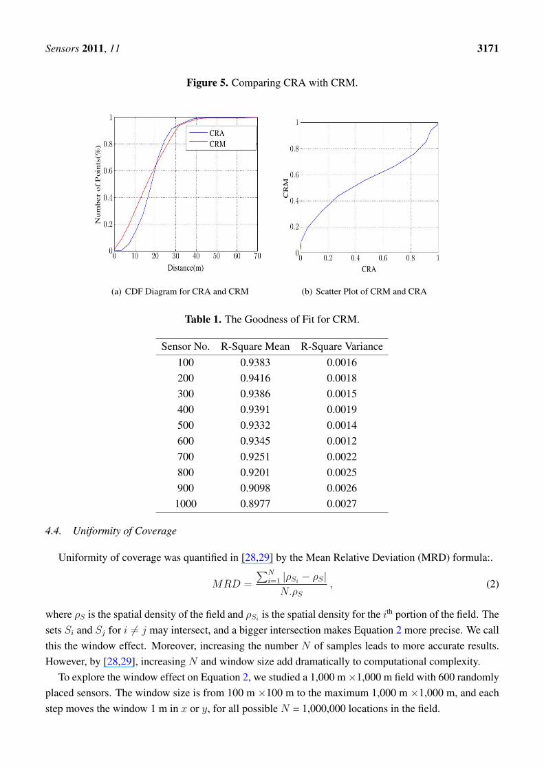
For CRA, we propose these steps. First, find the neighbors by a DT algorithm. Next, calculate theaverage value of do/ds for each triangle. These values are used as samples for the distances of all pointsof the field to their nearest sensors. The results show that the histogram of distribution of these samplepoints is very close to CRM (Figure 5). Moreover, it can be shown that the R-Square goodness of fitfrom CRA to true CRM is quite close to the perfect fit value 1. Table 1 is based on 1,000 random samplesfor each sensor density, in a 1,000 m ×1,000 m field.

Sensors 2011, 11 3171

Figure 5. Comparing CRA with CRM.

(a) CDF Diagram for CRA and CRM (b) Scatter Plot of CRM and CRA

Table 1. The Goodness of Fit for CRM.

Sensor No. R-Square Mean R-Square Variance100 0.9383 0.0016200 0.9416 0.0018300 0.9386 0.0015400 0.9391 0.0019500 0.9332 0.0014600 0.9345 0.0012700 0.9251 0.0022800 0.9201 0.0025900 0.9098 0.0026

1000 0.8977 0.0027

4.4. Uniformity of Coverage

Uniformity of coverage was quantified in [28,29] by the Mean Relative Deviation (MRD) formula:.

MRD =

∑Ni=1 |ρSi

− ρS|N.ρS

, (2)

where ρS is the spatial density of the field and ρSiis the spatial density for the ith portion of the field. The

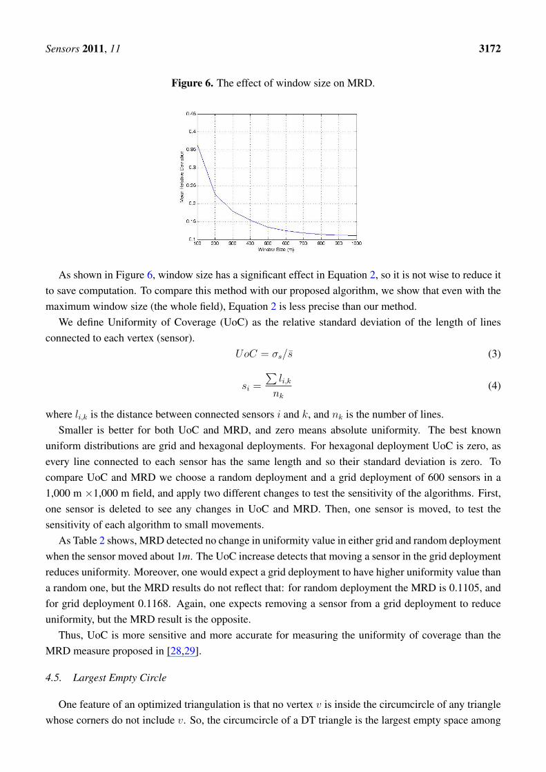
sets Si and Sj for i 6= j may intersect, and a bigger intersection makes Equation 2 more precise. We callthis the window effect. Moreover, increasing the number N of samples leads to more accurate results.However, by [28,29], increasing N and window size add dramatically to computational complexity.

To explore the window effect on Equation 2, we studied a 1,000 m×1,000 m field with 600 randomlyplaced sensors. The window size is from 100 m ×100 m to the maximum 1,000 m ×1,000 m, and eachstep moves the window 1 m in x or y, for all possible N = 1,000,000 locations in the field.

Sensors 2011, 11 3172

Figure 6. The effect of window size on MRD.

As shown in Figure 6, window size has a significant effect in Equation 2, so it is not wise to reduce itto save computation. To compare this method with our proposed algorithm, we show that even with themaximum window size (the whole field), Equation 2 is less precise than our method.

We define Uniformity of Coverage (UoC) as the relative standard deviation of the length of linesconnected to each vertex (sensor).

UoC = σs/s (3)

si =

∑li,knk

(4)

where li,k is the distance between connected sensors i and k, and nk is the number of lines.Smaller is better for both UoC and MRD, and zero means absolute uniformity. The best known

uniform distributions are grid and hexagonal deployments. For hexagonal deployment UoC is zero, asevery line connected to each sensor has the same length and so their standard deviation is zero. Tocompare UoC and MRD we choose a random deployment and a grid deployment of 600 sensors in a1,000 m ×1,000 m field, and apply two different changes to test the sensitivity of the algorithms. First,one sensor is deleted to see any changes in UoC and MRD. Then, one sensor is moved, to test thesensitivity of each algorithm to small movements.

As Table 2 shows, MRD detected no change in uniformity value in either grid and random deploymentwhen the sensor moved about 1m. The UoC increase detects that moving a sensor in the grid deploymentreduces uniformity. Moreover, one would expect a grid deployment to have higher uniformity value thana random one, but the MRD results do not reflect that: for random deployment the MRD is 0.1105, andfor grid deployment 0.1168. Again, one expects removing a sensor from a grid deployment to reduceuniformity, but the MRD result is the opposite.

Thus, UoC is more sensitive and more accurate for measuring the uniformity of coverage than theMRD measure proposed in [28,29].

4.5. Largest Empty Circle

One feature of an optimized triangulation is that no vertex v is inside the circumcircle of any trianglewhose corners do not include v. So, the circumcircle of a DT triangle is the largest empty space among

Sensors 2011, 11 3173

Table 2. Comparing UoC and MRD methods.

Random Deployment Grid DeploymentUoC MRD UoC MRD

Normal 0.6325 0.1105 0.0644 0.1168Movement (1 m) 0.6324 0.1105 0.0646 0.1168Movement (10 m) 0.6321 0.1104 0.0650 0.1168Removing one sensor 0.6321 0.1101 0.0654 0.1160

three vertices, or in other words, three sensors. This concept has already been used by [20], as the LargestEmpty Circle (LEC), to determine the best position for the next sensor deployment. Here, we proposethis property to find the largest uncovered area in a WSN.

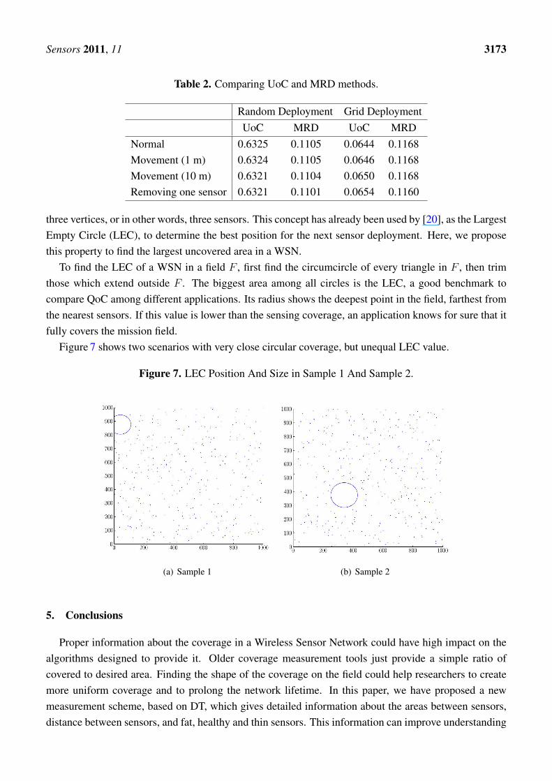
To find the LEC of a WSN in a field F , first find the circumcircle of every triangle in F , then trimthose which extend outside F . The biggest area among all circles is the LEC, a good benchmark tocompare QoC among different applications. Its radius shows the deepest point in the field, farthest fromthe nearest sensors. If this value is lower than the sensing coverage, an application knows for sure that itfully covers the mission field.

Figure 7 shows two scenarios with very close circular coverage, but unequal LEC value.

Figure 7. LEC Position And Size in Sample 1 And Sample 2.

(a) Sample 1 (b) Sample 2

5. Conclusions

Proper information about the coverage in a Wireless Sensor Network could have high impact on thealgorithms designed to provide it. Older coverage measurement tools just provide a simple ratio ofcovered to desired area. Finding the shape of the coverage on the field could help researchers to createmore uniform coverage and to prolong the network lifetime. In this paper, we have proposed a newmeasurement scheme, based on DT, which gives detailed information about the areas between sensors,distance between sensors, and fat, healthy and thin sensors. This information can improve understanding

Sensors 2011, 11 3174

of the coverage properties of different coverage promising algorithms, and comparison among them.This work is funded by Fundamental Research Grant Scheme (FRGS) under project number 78458.

References

1. Liu, T.; Li, Z.; Xia, X.; Luo, S. Shadowing Effects and Edge Effect on Sensing Coverage forWireless Sensor Networks. In Proceedings of 2009 5th International Conference on WirelessCommunications, Networking & Mobile Computing, Beijing, China, September 24–26, 2009;pp. 1–4.

2. Zhang, H.; Nixon, P.; Dobson, S. Partial Coverage in Homological Sensor Networks.In Proceedings of 2009 IEEE International Conference on Wireless and Mobile Computing,Networking and Communications, Marrakech, Morocco, October 12–14, 2009; pp. 42–47.

3. Chizari, H.; Abd Razak, S.; Arifah, B.; Abdullah, A.H. Deployment Density Estimationfor a-Covering Problem in Wireless Sensor Network. In Proceedings of 4th InternationalSymposium on Information Technology (ITSIM’10), Kuala Lumpur, Malaysia, June 15–17, 2010;pp. 592–596.

4. Chen, H.; Wu, H.; Tzeng, N.F. Grid-Based Approach for Working Node Selection in WirelessSensor Networks. In Proceedings of IEEE International Conference on Communications(IEEE Cat. No.04CH37577), University of Louisiana, Lafayette, LN, USA, June 20–24, 2004;pp. 3673–3678.

5. Parikh, S.; Vokkarane, V.M.; Xing, L.; Kasilingam, D. Node-Replacement Policies to MaintainThreshold-Coverage in Wireless Sensor Networks. In Proceedings of 16th InternationalConference on Computer Communications and Networks, Honolulu, HI, USA, August 13–16,2007; pp. 760–765.

6. Song, P.; Li, J.; Li, K.; Sui, L. Researching on Optimal Distribution of Mobile Nodes in WirelessSensor Networks being Deployed Randomly. In Proceedings of International Conferenceon Computer Science and Information Technology, Singapore, August 29–September 2, 2008;pp. 322–326.

7. Mao, Y.; Wang, Z.; Liang, Y. Energy Aware Partial Coverage Protocol in Wireless SensorNetworks. In Proceedings of International Conference on Wireless Communications, Networkingand Mobile Computing, Shanghai, China, September 21–25, 2007; pp. 2535–2538.

8. Tran-Quang, V.; Miyoshi, T. A novel gossip-based sensing coverage algorithm for dense wirelesssensor networks. Comput. Netw. 2009, 53, 2275–2287.

9. Tsai, Y.R. Sensing coverage for randomly distributed wireless sensor networks in shadowedenvironments. IEEE Trans. Veh. Technol. 2008, 57, 556–564.

10. Ghosh, A.; Das, S. Coverage and connectivity issues in wireless sensor networks: A survey.Pervasive Mob. Comput. 2008, 4, 303–334.

11. Wang, Q.; Xu, K.; Takahara, G.; Hassanein, H. WSN04-1: Deployment for Information OrientedSensing Coverage in Wireless Sensor Networks. In Proceedings of IEEE Globecom 2006, SanFrancisco, CA, USA, November 27–December 1, 2006; pp. 1–5.

Sensors 2011, 11 3175

12. Xing, G.; Tan, R.; Liu, B.; Wang, J.; Jia, X.; Yi, C.W. Data Fusion Improves the Coverageof Wireless Sensor Networks. In Proceedings of the 15th Annual International Conferenceon Mobile Computing and Networking, MobiCom’09, Beijing, China, September 20–30, 2009;pp. 57–168.

13. Mao, Y.; Zhou, X.; Zhu, Y. An Energy-Aware Coverage Control Protocol for WirelessSensor Networks. In Proceedings of International Conference on Information and Automation,Changsha, China, June 20–23, 2008; pp. 200–205.

14. Soreanu, P.; Volkovich, Z. Energy-Efficient Circular Sector Sensing Coverage Model for WirelessSensor Networks. In Proceedings of Third International Conference on Sensor Technologies andApplications, Athens, Glyfada, Greece, June 18–23, 2009; pp. 229–233.

15. So, A.; Ye, Y. On solving coverage problems in a wireless sensor network using Voronoi diagrams.Int. Netw. Econ. 2005, 3828, 584–593.

16. Boukerche, A.; Fei, X. A Voronoi Approach for Coverage Protocols in Wireless Sensor Networks.In Proceedings of IEEE GLOBECOM 2007-2007 IEEE Global Telecommunications Conference,Washington, DC, USA, November 26–30, 2007; pp. 5190–5194.

17. Aziz, N.A.B.A.; Mohemmed, A.W.; Alias, M.Y. A Wireless Sensor Network CoverageOptimization Algorithm Based on Particle Swarm Optimization and Voronoi Diagram. InProceedings of International Conference on Networking, Sensing and Control, Okayama, Japan,March 26–29, 2009; pp. 602–607.

18. Meguerdichian, S.; Koushanfar, F.; Potkonjak, M.; Srivastava, M. Coverage Problems in Wirelessad-hoc Sensor Networks. In Proceedings of Twentieth Annual Joint Conference of the IEEEComputer and Communications Society, IEEE INFOCOM 2001, Anchorage, AK, USA, April22–26, 2001; pp. 1380–1387.

19. Axler, S.; Ribet, K.A. Combinatorics and graph theory. In Undergraduate Texts in Mathematics;Springer: NY, New York, NY, USA, 2008.

20. Wu, C.H.; Lee, K.; Chung, Y. A Delaunay triangulation based method for wireless sensor networkdeployment. Comput. Commun. 2007, 30, 2744–2752.

21. Wang, J.; Medidi, S. Energy Efficient Coverage with Variable Sensing Radii in Wireless SensorNetworks. In Proceedings of Third IEEE International Conference on Wireless and MobileComputing, Networking and Communications (WiMob 2007), White Plains, NY, USA, October8–10, 2007; p. 61.

22. Vu, C.T.; Li, Y. Delaunay-Triangulation Based Complete Coverage in Wireless SensorNetworks. In Proceedings of 2009 IEEE International Conference on Pervasive Computing andCommunications, Galveston, TX, USA, March 9–13, 2009; pp. 1–5.

23. Calinescu, G. Localized delaunay triangulation with application in ad hoc wireless networks.IEEE Trans. Parall. Distrib. Sys. 2003, 14, 1035–1047.

24. Satyanarayana, D.; Rao, S. Local Delaunay Triangulation for Mobile Nodes. In Proceedingsof First International Conference on Emerging Trends in Engineering and Technology, Nagpur,Maharashtra, India, July 16–18, 2008; pp. 282–287.

25. Satyanarayana, D.; Rao, S.V. Constrained Delaunay Triangulation for ad hoc Networks.J. Comput. Syst. Netw. Commun. 2008, 2008, 1–11.

Sensors 2011, 11 3176

26. Araujo, F.; Rodrigues, L. Single-step creation of localized Delaunay triangulations. Wirel. Netw.2007, 15, 845–858.

27. Rahman, M.; Hussain, S. Uniformity and Efficiency of a Wireless Sensor Network’s Coverage.In Proceedings of 21st International Conference on Advanced Networking and Applications(AINA ’07), Niagara Falls, NY, USA, May 21–23, 2007; pp. 506–510.

28. Nittel, S.; Trigoni, N.; Ferentinos, K.; Neville, F.; Nural, A.; Pettigrew, N. A Drift-Tolerant Modelfor Data Management in Ocean Sensor Networks. In Proceedings of the 6th ACM internationalworkshop on Data engineering for wireless and mobile access, MobiDE ’07, Beijing, China, June10–12, 2007; pp. 49–58.

29. Ferentinos, K.; Tsiligiridis, T. Adaptive design optimization of wireless sensor networks usinggenetic algorithms. Comput. Netw. 2007, 51, 1031–1051.

30. De Berg, M.; Cheong, O.; Van Kreveld, M.; Overmars, M. Computational Geometry: Algorithmsand Applications; Springer-Verlag: New York, NY, USA, 2008.

31. Hjelle, Ø.; Dæhlen, M. Triangulations and Applications; Springer: New York, NY, USA, 2009.

c© 2011 by the authors; licensee MDPI, Basel, Switzerland. This article is an open access articledistributed under the terms and conditions of the Creative Commons Attribution license(http://creativecommons.org/licenses/by/3.0/.)