DEGREE PROJECT AT CSC, KTH The Effects of Dot Uniformity on ...

DEGREE PROJECT AT CSC, KTH

The Effects of Dot Uniformity on Halftone Mottle in Flexographic Prints on Coated Board

Kalicinski, Simon

KTH e-mail: [email protected]

Degree project in: Media Technology

Supervisors: Rosenqvist, Christopher

Thorman, Sofia

Yang, Li

Examiner: Li, Haibo

Project provider: Innventia AB

Abstract Flexographic print is a technology that is growing in popularity, especially in the packaging industry, due to its ability of printing on a wide variety of substrate types. Advances in ensuring good quality from flexographic processes have helped to bolster flexographic printing’s limited usage in the past decades. However, improving the quality of flexographic print products to a level that matches that of other mainstream printing methods is still needed. One common defect that affects flexographic print quality is mottling, which has been studied extensively in e.g. offset prints. At Innventia, a dependable method of calculating mottle numerically that highly correlates with subjective observations has been researched. This method has been applied into developing software called STFI-Mottle, which processes scanned images of halftones and returns average mottle values for them. In the case of this thesis, the goal has been to investigate what sort of characteristics in halftones caused by flexographic lead to a diminished halftone print quality on coated kraft board substrates. These characteristics were studied by examining dot uniformity in pre-printed samples of 30% halftone prints, then evaluating the data gathered with the ambition of finding a correlation between dot feature variations and print mottle. The mottle values that were used for analysis and discussion were computed using STFI-Mottle.

The initial reasoning was that “white spots” found within the samples’ raster dots should be closely examined, as they might provide clues to explaining unexpected print mottle. The 30% halftone cyan regions of printed samples were scanned with a high-resolution Creo iQsmart3 scanner. Next, a dot uniformity analysis was done with Matlab-based dot property calculation software. Thresholding was employed in image analysis in order to separate printed dots from unprinted substrate surface. A mottle evaluation was performed, focusing on the mottle values that were measured in the R channel using the same RGB images that were produced during scanning. Every data variable was compiled into a mean average for each sample, based on five to three signatures. Distribution histograms, simple linear regression and multiple linear regression were used to find meaningful correlations between measured data and mottle values.

The study resulted in some significant correlations between variables established as quality indicators, but also showed possible new connections between variables that can express dot uniformity and print mottle. Some variables’ viability as mottle predictors has been rejected, while others are presented as new opportunities for study. The deeper implications of some of the variables analysed could not be investigated, but a foundation for a methodology to conduct similar research has been laid. Furthermore, the thesis has yielded an initial base of knowledge on new objective data that might be used as alternative measurements for quantifying print quality. In conclusion, the study indicated that there are dot uniformity variables that can be linked to print mottle, if not by themselves, then using various combinations of them. Future research may determine the most accurate way that they can accomplish this.

Sammanfattning Flexografi är en tryckteknik som växer i popularitet, i synnerhet inom förpackningsindustrin, till följd av dess förmåga att trycka på ett brett urval av substrat. Framsteg inom kvalitetssäkring av produkter från flexografiprocesser har hjälpt till att öka flexografins begränsade användning från tidigare decennier. Förbättrandet av kvaliteten på produkter skapade med flexografi har dock fortfarande inte lett till en nivå som motsvarar andra vitt använda trycktekniker. En vanlig defekt som påverkar kvaliteten i flexotryck är flammighet, vars uppkomst har genomgått omfattande studier inom t. ex. offsettryck. På Innventia har en beprövad metod för att beräkna ett numeriskt värde på flammighet, som korrelerar väl med subjektivt uppmäta bedömningar, utvecklats genom forskning. Denna metodik har använts till att ta fram en mjukvara som kallas STFI-Mottle, som bearbetar skannade bilder av halvtoner och återger medelvärden för deras flammighet. I denna uppsats har målet varit att utreda vilken sorts egenskaper i halvtoner orsakade av flexotryck som går att härleda till en minskad tryckkvalitet på pilotbestruken kraftkartong. Dessa egenskaper undersöktes genom att utreda ”dot uniformity”, dvs. rasterpunkternas sammansättning, i förtryckta prover av 30% halvtoner. Sedan utvärderades den samlade data om dessa prover i syfte att hitta en korrelation mellan hur deras rasterpunkters sammansättning varierade och deras flammighet. Flammighetsvärdena som användes i analys och diskussion beräknades med hjälp av STFI-Mottle.

Det inledande resonemanget byggde på att “vita fläckar” som fanns i provernas rasterpunkter borde granskas noga, då detta skulle ge ledtrådar till en möjlig förklaring en oväntad hög nivå flammighet i vissa prover. De delar av proverna som innehöll 30% cyan halvtoner skannades med en högupplöst Creo iQsmart3-skanner. Därpå utförds en ”dot uniformity”-analys med hjälp av en MatLab-baserad mjukvara som beräknar rasterpunkters egenskaper. Tröskling användes i denna process för att kunna separera tryckta rasterpunkter från otryckt substratyta. En flammighetsutvärdering gjordes i R-kanalen på de RGB-bilder som fåtts genom skanning. KoHistogram, linjär regressionsanalys samt multipel linjär regressionsanalys användes för att hitta intressanta korrelationer mellan samlad ”dot uniformity”-data och flammighetsvärden.

Studien gav upphov till några betydande korrelationer mellan variabler som ansågs indikera kvalitet enligt tidigare forskning, men visade även att det fanns nya möjliga kopplingar mellan variabler som kan uttrycka ”dot uniformity” och uppmätt flammighet i tryck. Somliga variablers trovärdighet i att förutspå flammighet har kunnat avfärdas inom ramarna för denna studie, medan andra presenteras som kandidater för vidare forskning. Djupare implikationer till följd av den analys som gjorts på variablerna i denna studie har inte utretts till fullo, men en grund till en metod för att utföra liknande forskning har lagts. Studien har också lett till en kunskapsbas om vad för sorts objektiv data som eventuellt kan användas som alternativa numeriska mått på tryckkvalitet. Sammanfattningsvis så tyder studien i denna uppsats på att det finns variabler för ”dot uniformity” som, om inte enskilt så åtminstone i olika konstellationer, kan kopplas ihop med flammighet. Framtida forskning kan möjligen avgöra det mest noggranna sättet att åstadkomma en sådan anknytning.

Acknowledgements I would like to thank my supervisors at Innventia, Sofia Thorman and Li Yang, for their guidance, input, thoughts and conversations that have taught me many things and doubtlessly strengthened my work. My supervisor at KTH, Christopher Rosenquist, also deserves thanks for his feedback and help in the completion of this thesis.

I also want to thank Anita Teleman for welcoming me to Innventia and laying the foundation for a master’s thesis to be written.

Lastly, I want to extend my gratitude to Hans Christiansson of Innventia AB for his invaluable aid and problem-solving skills, without which there might never have been a finished thesis in its present form.

Simon Kalicinski, May 2014

Index 1.   Introduction ..................................................................................................................................... 1  

1.1.   Background ............................................................................................................................... 1  1.2.   Study goals ............................................................................................................................... 1  

2.   Theory .............................................................................................................................................. 2  2.1.   Flexographic Printing ............................................................................................................... 2  2.2.   Halftones & Rasters .................................................................................................................. 2  2.3.   Coating ...................................................................................................................................... 3  2.4.   Print Quality ............................................................................................................................. 3  2.5.   Print Mottle ............................................................................................................................... 4  2.6.   Dot Gain ................................................................................................................................... 4  2.7.   Dot Roundness and Dot Fidelity .............................................................................................. 5  2.8.   Image Analysis ......................................................................................................................... 5  

2.8.1.   Thresholding ...................................................................................................................... 5  2.8.2.   Reflectance Variations ....................................................................................................... 6  

3.   Method ............................................................................................................................................. 7  3.1.   Materials ................................................................................................................................... 7  3.2.   Printing Conditions ................................................................................................................... 7  3.3.   Previous Findings ..................................................................................................................... 7  3.4.   Visual Examination .................................................................................................................. 8  3.5.   Sample Scans ............................................................................................................................ 8  3.6.   Image Analysis: Dot Uniformity .............................................................................................. 9  

3.6.1.   Data Variables ................................................................................................................. 12  3.6.2.   Additional Variables ........................................................................................................ 13  

3.7.   Image Analysis: Mottle Evaluation ........................................................................................ 13  4.   Results ........................................................................................................................................... 15  

4.1.   Dot Uniformity Analysis ........................................................................................................ 15  4.2.   Print Mottle Evaluation .......................................................................................................... 17  4.3.   Dot Distributions .................................................................................................................... 21  4.4.   Multiple Linear Regression Analysis ..................................................................................... 25  

5.   Discussion ...................................................................................................................................... 28  6.   Conclusion ..................................................................................................................................... 30  7.   Application .................................................................................................................................... 32  8.   Resources ....................................................................................................................................... 33  9.   Appendices .................................................................................................................................... 34  

9.1.   Appendix I: Scanning With Creo iQsmart3 ............................................................................ 34  9.2.   Appendix II: DotStat Analysis ............................................................................................... 38  9.3.   Appendix III: Full Width at Half Maximum .......................................................................... 40  9.4.   Appendix IV: MLR Analysis Progression .............................................................................. 41  

Table of Figures Fig A Left: schematic illustration of flexographic print system, right: magnified microscope image of anilox roller surface. ............................................................................................................................... 2  Fig B An example of a black to white linear gradient (below) and a rasterized halftone version (above). ................................................................................................................................................... 3  Fig C A scanned image of the entire 30B:1 signature, the 30% halftone with normal ink application is seen bottom left. ...................................................................................................................................... 7  Fig D Dot types noticed in visual assessment of signatures with varying mottle, here magnified by a factor 75 through a microscope lens. The left signature crop has more intact and uniform raster dots than the one on the right. ......................................................................................................................... 8  Fig E A scanned image of the reflectance calibration frame. ............................................................... 10  Fig F Example of reflectance calibration plot. ..................................................................................... 10  Fig G Example of DotStat plotting an optimal threshold value in an image’s pixel reflectance levels histogram. .............................................................................................................................................. 11  Fig H Example of difference in dot object appearances after using Erode/Dilate. Left: a binary image before initializing the Erode/Dilate function. Right: the same image after Erode/Dilate has been used, note the “open” dot objects. .................................................................................................................. 12  Fig I Example of band pass filters displaying different scales of mottle. The original image includes all subsets of wavelength bands. Red and blue areas represent higher and lower reflectance, respectively. Note the “grainier” variations in the 0.25-0.5 mm band and the “cloudlike” variations in the 1-2 mm band. .................................................................................................................................. 13  Fig J The correlation between dot gain and mean dot area over the whole sample range gives a coefficient of determination of 0.83, which is considerably high. The ranking among samples based on mean dot area is very similar to their ranking in relation to their measured dot gain. ..................... 15  Fig K The correlation between shape factor and standard deviation of reflectance in a dot’s pixels show an expected negative trend, with a coefficient of determination that is reasonably high. ........... 16  Fig L A positive correlation of the average standard deviation of the pixel reflectance values in a sample’s dots with the presence of “white spots” in the same dots links the reflective homogeneity of a sample’s raster dots with ink coverage defects that were noticed through loop magnification. ........ 16  Fig M The figure shows an excellent correlation, reinforcing a notion that the samples where more dots contain “white spots” also have the largest “white spots” on average. ......................................... 17  Fig N This figure contains the mean mottle values in the R channel of RGB. ..................................... 18  Fig O A correlation plot between sample mottle and average standard deviation in dot reflectance, where the trend lines have been marked out for sample groups based on coating compositions. ........ 18  Fig P The correlations seen here differ strongly between the sample groups; one unexpectedly displays a negative trend. ...................................................................................................................... 19  Fig Q Shape factor’s correlation with mottle is shown for the aforementioned sample groups made in the 2011 study. ...................................................................................................................................... 19  Fig R The correlation is shown between mottle in the 1-8 mm wavelength band and a quotient of the variables Darkest 10% and Avg Reflectance. This quotient describes how high the sample mean for the average reflectance of the 10% darkest pixels of every dot in a sample is in relation to the sample mean for the average reflectance for every dot as a whole. .................................................................. 20  Fig S The Relative Brightest 10% variable shows how great the reflectance is for a dot’s 10% brightest pixels relation to the dot’s overall average reflectance. This variable correlates badly with mottle, possibly much due to samples that visibly deviate from the linear model. .............................. 21  Fig T This figure contains instances of histograms that display characteristics one can draw conclusions from by visual assessment. For example, it is evident that the histograms of signature 38B:5 and 40B:5 differ in width around their peaks, and consequently one has a more homogenously

distributed dot population with regards to their standard deviation in reflectance. Such conclusions can arguably also be expressed in numerical terms. ............................................................................. 22  Fig U The correlation here shows the relation between how greatly the reflectance in a sample’s dots varies on average and how strongly on average this variation varies between all the dots in the samples signatures. ................................................................................................................................ 22  Fig V White spot area is related to how strongly the average reflectances of dots vary within a sample. ............................................................................................................................................................... 23  Fig W The FWHM Avg Reflectance measurement gives an understanding of how much a sample’s dots vary in mean reflectance. Considering the theory discussed on mottle quantifies it as variations in reflectance, measured mottle should increase with higher FWHM Avg Reflectance. ......................... 23  Fig X The correlation of mottle with FWHM StdDev Reflectance bears a close resemblance to that of Fig W, and has its fit to a linear model similarly negatively affected by a few deviating samples. ..... 24  Fig Y Among samples, the variation in reflectance standard deviation among dots correlates quite highly with the variation of the average reflectance of those dots. ....................................................... 25  Fig Z Here 𝑌𝑖 is based on values Amount “White Spots” and Avg "White Spot" Area. ..................... 26  Fig AA A Correlation diagram between FWHM Reflectance and 𝑌𝑖 values gained from MLR combination of three different data gained from dot uniformity analysis: StdDev Reflectance, average “white spot” area and the quotient of the variables Darkest 10% and Avg Reflectance. ..................... 26  Fig BB A Correlation diagram between print mottle in the 1-8 mm band and 𝑌𝑖 values gained from MLR combination of three different variables gained from dot uniformity analysis: FWHM StdDev Reflectance, FWHM Avg Reflectance and Shape Factor. .................................................................... 27  

1

1. Introduction

1.1. Background Flexographic is a printing method that is known for its versatility in application on various non-paper substrates, for instance, on board materials frequently used in packaging. As the use of flexographic is increasing in the print industry, the need to ensure that it delivers an acceptable print quality is of great importance. A high quality print gives an important impression to a consumer that judges the final product at the end of distribution. Research into print quality assurance and quality control is an integral part of the printing industry, yet at the moment of writing research into the underlying effects on print mottle in flexographic print products is in an evolving state, and there is much knowledge left to be gained. Flexographic is not unique in this regard; a standard numerical value to universally describe print quality that is widely accepted in the printing industry has yet to be invented and applied in any printing method. This study was carried out at the facilities of Innventia AB (formerly STFI-Packforsk) within their Packaging Solutions and Material Processes department. The aim was to expand knowledge on ensuring an acceptable print quality in flexographic productions for packaging materials.

1.2. Study goals This thesis explores the possibility of registered print mottle correlating with data variables produced from analysis of halftone dots that were printed using flexographic. An inverse correlation between print mottle and dot gain has previously been found using the same printed samples that acted as material in the study. Print mottle is a parameter that is frequently measured and judged in all manner of print processes, and is easily noticed by the casual observer. Mottle is one possible factor in examining a print that describes print quality. Unfortunately, in the evaluations that prelude this study it has not conformed to an expected correlation with registered dot gain. Therefore, the basis of this thesis is an interest in whether mottle levels might be attributed to factors that are not seen in visual assessment or that have not been sought previously.

Furthermore, the various coating compositions used for the printing of samples caused a varying absorption factor in the substrates. The predicted trend was that a higher absorption factor would lead to lower print mottle, but this also proved to be false. Absorption factor and mottle showed a mostly positive correlation for the evaluated samples. The opinion was that a more extensive study of possible additional causes of mottle is required. Hopefully, new insights can be gained using image analysis and a more detailed examination of dot properties.

An attempt was made to establish new connections between micro-scale features in flexographic prints with objectively measured mottling on a macro level. The idea is to examine how unnoticed features might contribute to certain prints being perceived as being of lower quality as a consequence of print mottle. Similar research has been carried out on, for instance, inkjet prints that are subject to additional other defects but have their quality evaluated with largely the same principles.

2

2. Theory

2.1. Flexographic Printing Flexographic is a direct printing method, which means that the flexographic cliché transfers ink directly to the substrate, or print surface. The cliché is made from either rubber or a polymer compound and is therefore quite malleable. As a consequence, this requires that the impression cylinder is rigid, since it creates the counter-force that allows for the cliché to apply ink to the print material with equal contact. (Johansson et al, 2008)

An undeveloped polymer cliché has a photosensitive surface that hardens when exposed to light. In the platemaking process, the undeveloped cliché can be either covered with a film negative and then exposed to ultraviolet light or engraved with a computer-controlled laser (digital platemaking). The cliché is then washed with either water or solvent to remove the unexposed polymer, leaving “raised” areas that will transfer ink during printing. (Johansson et al, 2008)

Flexographic is often applied on materials with low absorption factors and as such, the inks used have to dry relatively quickly once applied to the substrate. Therefore, the fast-drying inks must be effectively transported from the ink tank to the cliché roll. The ink roll is partially immersed in the ink tank, and successively transfers the ink to the anilox roll. The anilox roll has a cell-structured surface that is covered with a pattern of microscopic depressions (or cups) that pick up ink more effectively than a flat roll (see Error! Not a valid bookmark self-reference.). A scraper, or doctor blade, is applied to the anilox roll in order to remove excess ink before it is transferred to the cliché roll (see Error! Not a valid bookmark self-reference.). This ensures that an even ink application can be ensured at a good speed. (Johansson, 2008)

2.2. Halftones & Rasters Most printing presses are not capable of reproducing continuous tonal shifts, since they operate on a virtually binary premise of either applying ink or not. This means that a lighter tone cannot be created by e.g. adjusting the thickness of an ink layer about to be applied to a substrate. Instead, images with gradually shifting tonalities are split into small components that are not individually discernible to the naked eye. (Johansson et al, 2008)

Fig A Left: schematic illustration of flexographic print system, right: magnified microscope image of anilox roller surface.

3

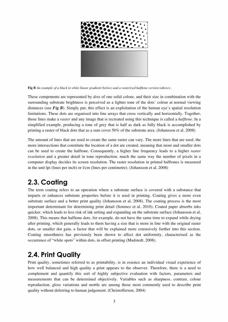
Fig B An example of a black to white linear gradient (below) and a rasterized halftone version (above).

These components are represented by dots of one solid colour, and their size in combination with the surrounding substrate brightness is perceived as a lighter tone of the dots’ colour at normal viewing distances (see Fig B). Simply put, this effect is an exploitation of the human eye’s spatial resolution limitations. These dots are organised into line arrays that cross vertically and horizontally. Together, those lines make a raster and any image that is recreated using this technique is called a halftone. In a simplified example, producing a tone of grey that is half as dark as fully black is accomplished by printing a raster of black dots that as a sum cover 50% of the substrate area. (Johansson et al, 2008)

The amount of lines that are used to create the same raster can vary. The more lines that are used, the more intersections that constitute the location of a dot are created, meaning that more and smaller dots can be used to create the halftone. Consequently, a higher line frequency leads to a higher raster resolution and a greater detail in tone reproduction, much the same way the number of pixels in a computer display decides its screen resolution. The raster resolution in printed halftones is measured in the unit lpi (lines per inch) or l/cm (lines per centimetre). (Johansson et al, 2008)

2.3. Coating The term coating refers to an operation where a substrate surface is covered with a substance that imparts or enhances substrate properties before it is used in printing. Coating gives a more even substrate surface and a better print quality (Johansson et al, 2008). The coating process is the most important determinant for determining print detail (Sonmez et al, 2010). Coated paper absorbs inks quicker, which leads to less risk of ink setting and expanding on the substrate surface (Johansson et al, 2008). This means that halftone dots, for example, do not have the same time to expand while drying after printing, which generally leads to them having a size that is more in line with the original raster dots, or smaller dot gain, a factor that will be explained more extensively further into this section. Coating smoothness has previously been shown to affect dot uniformity, characterised as the occurrence of “white spots” within dots, in offset printing (Madstedt, 2008).

2.4. Print Quality Print quality, sometimes referred to as printability, is in essence an individual visual experience of how well balanced and high quality a print appears to the observer. Therefore, there is a need to complement and quantify this sort of highly subjective evaluation with factors, parameters and measurements that can be determined objectively. Variables such as sharpness, contrast, colour reproduction, gloss variations and mottle are among those most commonly used to describe print quality without deferring to human judgement. (Christofferson, 2004)

4

A common unit that is associated with controlling print quality is reflectance, defined as the amount of incoming light that is reflected by a specific print or part of a print (Johansson et al, 2008). It is usually expressed in percent light reflected and assigned the unit [%]. Reflectance is a component of calculating print density, which is a similar measurement, but one that rather makes use of reflectance to express the properties of individual printed colours in reference to a corresponding control value. Reflectance by itself, on the other hand, is theoretically intended to describe print properties in relation to what the human observer perceives, hence its potential suitability in applying numerical values to subjective observations. Despite this, a widely accepted industry standard parameter that universally describes print quality has yet to be invented or introduced.

2.5. Print Mottle Print mottle is an important characteristic to quantify print quality and printability (Sonmez et al, 2010). Print mottle can be thought of as reflectance disturbances in the print that lead to a deterioration in the perceived quality of the print (Fahlcrantz, 2005), or as an undesirable variation in print density in a printed image that is evaluated by either visual assessment or image analysis (Ragnarsson, 2012 & Johansson, 1993). The amount of print mottle that is measured or observed can be linked to mean reflectance levels (Fahlcrantz, 2005). In this study mottle is defined as a spatial variation of reflectance levels, which can be examined within different wavelength bands.

To the casual observer, print mottle can generally take on either random or ordered forms. A random type of print mottle presents itself as clouds on a larger scale or grains on a smaller scale. More regular forms of print mottle can be seen as straight lines and stripes of varying reflectance or other types of periodic patterns. Mottle can be very disturbing to the viewer as soon as a large area of homogenous tone are printed, but is less noticeable in rich, detailed images. In addition, the level of mottle may vary substantially between halftone and full tone prints, and is usually higher in the former than the latter. (Christofferson, 2004)

2.6. Dot Gain Dots in a halftone have a defined size in order to produce a design accurately in print. During printing, this size changes and the raster dots become larger than intended. This deformation is referred to as dot gain and generally leads to all printed tones becoming darker than in the original design, because the raster dots contain more ink and the amount of unprinted substrate that shows is lower. Dot gain is considered a useful variable for determining if a print process is stable, as it is expected to be reproduced consistently while other printing variables remain unchanged. (Johansson et al, 2008)

Dot gain is also a common factor in determining print quality. For instance, a low dot gain generally demonstrates high print quality. Additionally, dot gain is seen as a variable that correlates with print mottle measurements, especially if it applies non-uniformly to the print. In other words, if a halftone is printed and the raster dots are affected by dot gain to very varying degrees, that halftone may contain dark and light “patches” (clusters of enlarged or reduced raster dots). Generally, dot gain is affected by both the anilox roller and the plate for flexographic printing (Sonmez et al, 2010). It is in the so called nip, the surface of contact between rollers, that dot gain is usually caused as transferred ink is flattened. Flexographic has been known to cause quite substantial dot gain, partially because the printing areas of its “soft” cliché expand easily upon contact with the impression cylinder. In general, dot gain is a factor that the printing process is adapted to. There are usually actions taken to mitigate it (without the ambition to eliminate it), such as choice of printing method, substrate type, adjusting raster density, choice of raster types, or using coated substrates (Johansson et al, 2008).

5

2.7. Dot Roundness and Dot Fidelity Dot roundness is a method to characterize dot quality, and gives a good characterization of dots along with measured dot gain (Sonmez et al, 2010). How round a dot is speaks of how well its shape has been reproduced in print in comparison to the original rasterized image file. The shape, as well as the size of dots depends significantly on which substrate and coating are being used (Fleming, 2003) because of how it affects the substrates absorption properties. Dot fidelity is another important measurement in judging image quality that utilizes a combined analysis of dots’ nearness to circularity and how much their total areas vary (Fleming, 2003). Dot fidelity has previously been used in analysis of inkjet dots to determine print quality.

Collecting data about dot roundness and dot area requires advanced high-resolution scanner optics and computing software for it to be effectively carried out on print samples that are made with halftone rasters on a small scale that is true to reality. The challenge lies in finding and identifying individual dots in halftone prints, as well as knowing how to translate them into data. The scope of this data will then depend on the ability of the hardware to capture detailed and uncorrupted images of the regions of interest.

2.8. Image Analysis

2.8.1. Thresholding Digital image analysis facilitates an effective method to gather data on a larger scale about printed samples. In the case of analysing halftones, it is of importance to distinguish printed dots from unprinted substrate. This requires determining a pixel value boundary to associate pixels with either printed or unprinted areas, called image “thresholding”. There are different approaches to thresholding, but the method chosen will be clarified further on in this thesis.

One of the ways to gain valuable information on a halftone print is to study the histogram of the micro scale image of the halftone print (Namedanian, 2013). Halftone dot area, paper reflectance and dot reflectance are parameters that can be determined using halftone print image histograms (Namedanian, 2013). Such histograms display characteristic “dual” peaks, which represent unprinted paper base on the far right and printed halftone area on the far left. (Namedanian, 2013)

The use of histograms in images of printed halftones has previously been researched by analysing inkjet dots that are affected by a defect called “feathering” (or “wicking”). Feathering is an unwanted, often irregular, spread of ink on the substrate around the edges of a printed area. In a recent case, thresholding was used to identify inkjet printed areas that were of interest in gathering data for quality assessment. The thresholding was based on pixel luminance values (brightness) in 8-bit images that effectively could range from 0 to 255. A computing software was used to identify appropriate thresholds, apply them on inkjet dots in order to associate pixels into printed objects, and finally completed calculations of the luminance values, or brightness, of all those pixels that were regarded as being within the perimeter of a dot. (Habekost, 2013)

In this previous research, the standard deviation of mean pixel luminance was proposed as the basis of comparative measurement of substrate quality, as the variation in pixel luminance value within the dot perimeter was judged to be of primary interest. The dot circularity was also determined to show how this parameter corresponded with the mean pixel luminance standard deviation. The dot circularity was connected to pixel luminance standard deviation in the sense that rounder dots generally correlated with a lower standard deviation in pixel luminance. (Habekost, 2013)

6

2.8.2. Reflectance Variations The human visual system is sensitive to lateral sine wave patterns, and pixel value variations in digital images can be noted as having a spatial wavelength (Johansson, 1993). If pixel reflectance variations in an image are wavelengths, then it follows that appearances of mottling can also be noted as wavelengths. Mottling is often divided into different wavelength bands when processed in image analysis (Ragnarsson, 2012). At Innventia, this division has been split into wavelength bands between 0.25-16 mm, with the first band at 0.25-0.5 mm and consecutive band intervals being doubled compared to the previous one, up to the last band of 8-16 mm (Johansson, 1993).

In print mottle evaluation, the most important measurement of mottle levels falls within in the range of 1-8 mm. This span of wavelengths is emphasised and focused on because it contains measured defects that correlate most closely to ones that are subjectively observed (Johansson, 1993). For the sake of distinction we can state that “grain” mottle mostly falls within the 0.25-0.5 mm band (or even shorter wavelengths), and the spatial reflectance variations in the 1-8 mm band mostly resemble “cloud” mottle.

7

3. Method

3.1. Materials Fourteen pilot-coated boards were produced at Korsnäs Frövi, using a base board supplied by Klabin. The board was a three-layer construction with a top layer of bleached Kraft pulp and a grammage of 200g/m2

. The coating was done at 600m/min using a Jagenberg bent ceramic blade on the top layer. 12 gsm pre-coat and 12 gsm top-coat was applied to the top layer. The same pre-coating was used on all samples.

3.2. Printing Conditions The samples (numbered 30B-43B) were printed at Tetra Pak in Lund, Sweden on an in-line flexographic press. For each sample a total of six signatures was selected and numbered 1 to 6 (for instance sample no. 36 consists of six signatures labelled 36B:1, 36B:2, etc.) The press settings were adjusted for the first sample and subsequently kept constant for all other samples. The region of the sample signatures that was analysed in this thesis was a cyan 30% halftone printed with a standard ink amount and a printing resolution of 48 lines per cm. The ink used was provided by Siegwerk.

Fig C A scanned image of the entire 30B:1 signature, the 30% halftone with normal ink application is seen bottom left.

3.3. Previous Findings The basis for this study is an Innventia report from 2011 (No. 285) in which print mottle was evaluated in 30% cyan halftones using a flatbed scanner and STFI Mottling Expert software. The same halftones are analysed and discussed in this thesis. Five signatures from each sample were scanned with the Epson Perfection V750 Pro, with a resolution of 300 dpi. For some samples, one signature was deemed highly defective and discarded. If so, it was replaced with a sixth signature from the same sample. An average print mottle in the 30% cyan halftone was then calculated for each signature based on five sub-areas of the region. A sample mean was taken based on the values from five signatures. Other measurements partially discussed in this thesis from the previous Innventia were top coating compositions, ink absorption factor, dot gain and white-top mottle.

8

In this study, an inverse correlation between dot gain and print mottle in the 1-8 mm band was noted for a group of samples. In the report, the samples used were later grouped according to how the chemical content of their coating was varied. For instance, samples 38-40 had differing parts latex added to their coating and samples 34-37 had varying amounts of clay mixed into theirs. The coating compositions could offer explanations to certain findings, but their properties will not be explicitly attached to any findings in this thesis.

3.4. Visual Examination In the samples that were available, two particular sample series were initially selected for visual assessment. These were chosen on the basis of showing an inverse correlation between print mottle and dot gain. The two series consisted of three samples with five to six signatures each.

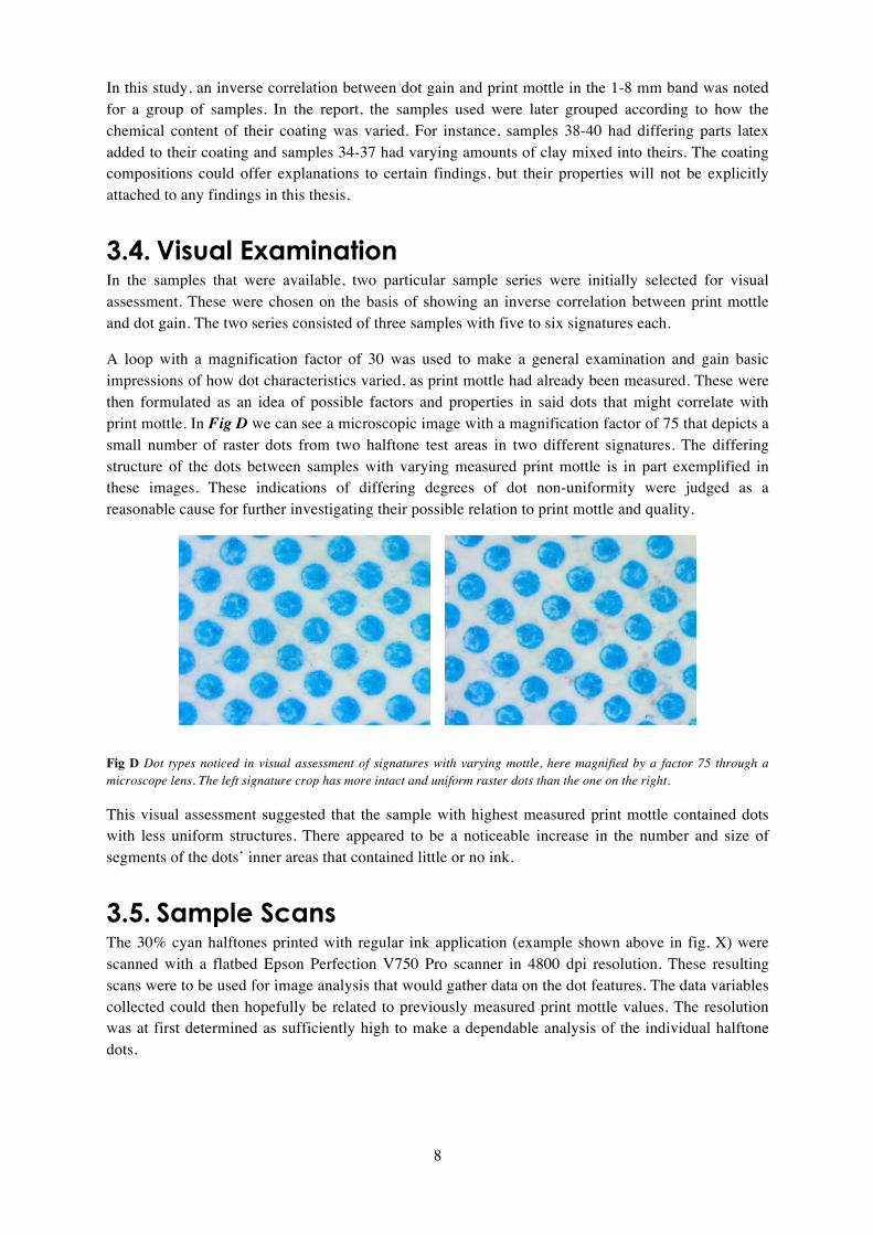
A loop with a magnification factor of 30 was used to make a general examination and gain basic impressions of how dot characteristics varied, as print mottle had already been measured. These were then formulated as an idea of possible factors and properties in said dots that might correlate with print mottle. In Fig D we can see a microscopic image with a magnification factor of 75 that depicts a small number of raster dots from two halftone test areas in two different signatures. The differing structure of the dots between samples with varying measured print mottle is in part exemplified in these images. These indications of differing degrees of dot non-uniformity were judged as a reasonable cause for further investigating their possible relation to print mottle and quality.

Fig D Dot types noticed in visual assessment of signatures with varying mottle, here magnified by a factor 75 through a microscope lens. The left signature crop has more intact and uniform raster dots than the one on the right.

This visual assessment suggested that the sample with highest measured print mottle contained dots with less uniform structures. There appeared to be a noticeable increase in the number and size of segments of the dots’ inner areas that contained little or no ink.

3.5. Sample Scans The 30% cyan halftones printed with regular ink application (example shown above in fig. X) were scanned with a flatbed Epson Perfection V750 Pro scanner in 4800 dpi resolution. These resulting scans were to be used for image analysis that would gather data on the dot features. The data variables collected could then hopefully be related to previously measured print mottle values. The resolution was at first determined as sufficiently high to make a dependable analysis of the individual halftone dots.

9

After some initial processing of scanned halftones through image analysis software, the conclusion was drawn that the images lacked the necessary sharpness and detail to provide enough information for samples to distinguish themselves clearly in the data. Consequently, it was decided that another process of scanning the samples would be initiated by using a CREO iQsmart3 scanner that possessed improved optics and detail reproduction, at the same resolution.

First and foremost, a hardware and system diagnostics was run for the CREO scanner in order to ensure standardised scanning in the future. When this was completed successfully, a preview low-resolution scan was made on a 30% halftone area of a sample signature. Now, certain scanner settings had to be adapted and set as a standard for all samples so that scanning would be efficient and uniform:

• End Points • Gradiation • Sharpness

The End Points function was used to define maximum brightest and darkest areas of scanned images. When set, this ensured that all scanned samples would contain pixel values that fit within the same interval. The Gradiation setting was used to adjust the image contrast. This was important so that image analysis software used could interpret the scanned samples as having sufficiently linear pixel value distribution (this will be explained further in the coming section). Sharpness was deactivated entirely as the consequences of using this function was unfamiliar to the study author at the moment of writing, and no clear reason for sharpening (and potentially distorting) scanned images presented itself.

For samples 38B through 43B five signatures per sample were scanned, and due to lack of time three signatures were scanned for each one of the remaining samples 30B through 37B. Every scan was further divided into three separate crops (numbered 1 to 3) that consisted of sub-areas located in the 30% halftone region of each signature. The calibration frame required by the image analysis software was also scanned with the same scanner settings as the samples but only at 300 dpi resolution. Each scanned sub-area was saved as a 24-bit RGB uncompressed TIFF image file.

3.6. Image Analysis: Dot Uniformity An image analysis program, referred to from this point on as DotStat, was used to compute and calculate data from the scanned images of raster dots. This program was a modified version of existing software developed at Innventia, created in MatLab with the specific purpose of being able to identify and analyse printed dots in images of scanned halftone raster prints. The main principle of this program was to identify all printed dots in an image, identify them as separate objects and create a binary image with pixels that would represent printed or unprinted surface of every identified dot. Thus, the whitespace of unprinted paper and unwanted defects needed to be clearly distinguished and separated from printed areas.

This was done by first converting the scanned RGB sample images into 8-bit Grayscale so that it could depict reflectance. In this conversion, solely RGB pixel data from the R (red) channel was used, as the test prints were made with cyan ink, which reproduces the widest pixel value distribution in the R channel of RGB. Therefore, a grayscale image based on the R channel would represent the most relevant information on pixel reflectance values for identified dots and could most accurately represent variations in reflectance with high detail.

10

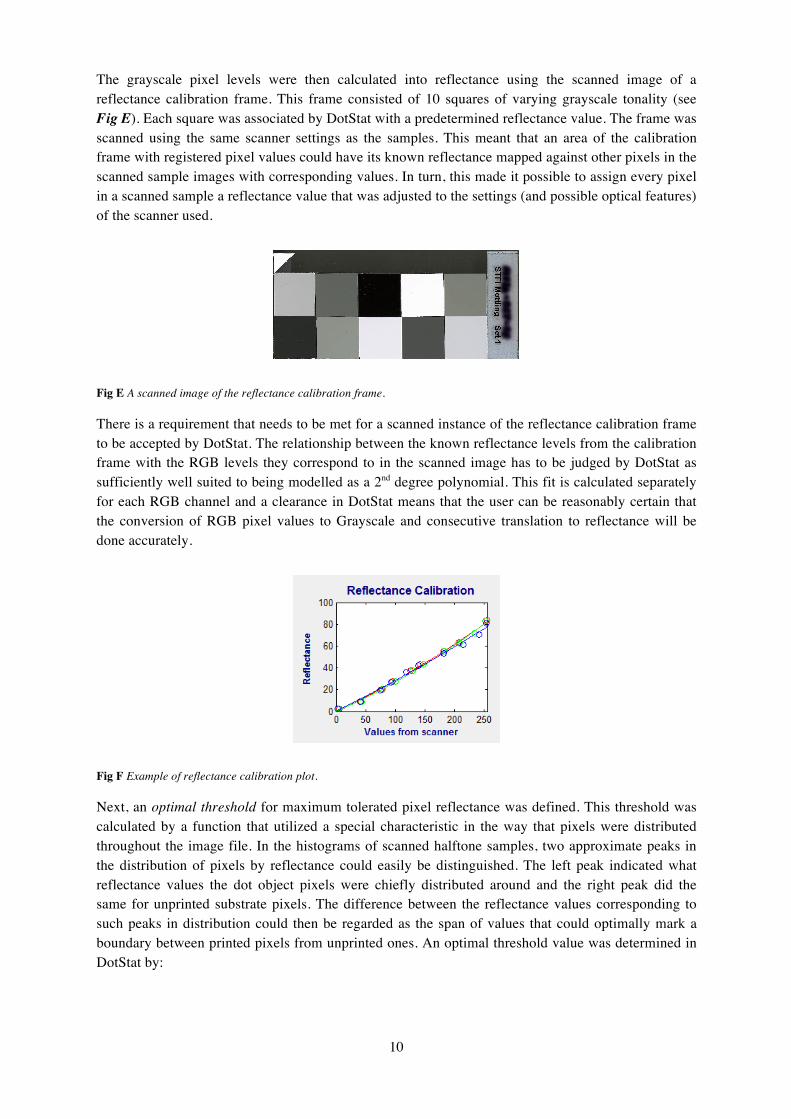
The grayscale pixel levels were then calculated into reflectance using the scanned image of a reflectance calibration frame. This frame consisted of 10 squares of varying grayscale tonality (see Fig E). Each square was associated by DotStat with a predetermined reflectance value. The frame was scanned using the same scanner settings as the samples. This meant that an area of the calibration frame with registered pixel values could have its known reflectance mapped against other pixels in the scanned sample images with corresponding values. In turn, this made it possible to assign every pixel in a scanned sample a reflectance value that was adjusted to the settings (and possible optical features) of the scanner used.

Fig E A scanned image of the reflectance calibration frame.

There is a requirement that needs to be met for a scanned instance of the reflectance calibration frame to be accepted by DotStat. The relationship between the known reflectance levels from the calibration frame with the RGB levels they correspond to in the scanned image has to be judged by DotStat as sufficiently well suited to being modelled as a 2nd degree polynomial. This fit is calculated separately for each RGB channel and a clearance in DotStat means that the user can be reasonably certain that the conversion of RGB pixel values to Grayscale and consecutive translation to reflectance will be done accurately.

Fig F Example of reflectance calibration plot.

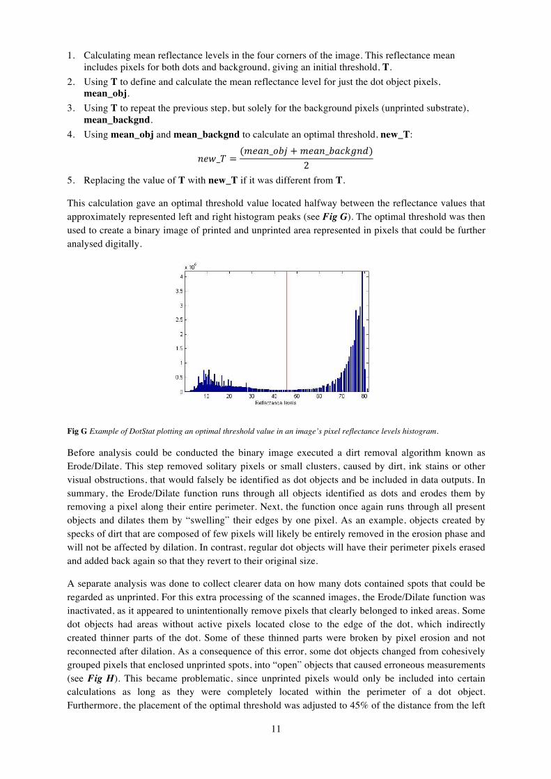
Next, an optimal threshold for maximum tolerated pixel reflectance was defined. This threshold was calculated by a function that utilized a special characteristic in the way that pixels were distributed throughout the image file. In the histograms of scanned halftone samples, two approximate peaks in the distribution of pixels by reflectance could easily be distinguished. The left peak indicated what reflectance values the dot object pixels were chiefly distributed around and the right peak did the same for unprinted substrate pixels. The difference between the reflectance values corresponding to such peaks in distribution could then be regarded as the span of values that could optimally mark a boundary between printed pixels from unprinted ones. An optimal threshold value was determined in DotStat by:

11

1. Calculating mean reflectance levels in the four corners of the image. This reflectance mean includes pixels for both dots and background, giving an initial threshold, T.

2. Using T to define and calculate the mean reflectance level for just the dot object pixels, mean_obj.

3. Using T to repeat the previous step, but solely for the background pixels (unprinted substrate), mean_backgnd.

4. Using mean_obj and mean_backgnd to calculate an optimal threshold, new_T:

𝑛𝑒𝑤_𝑇 =(𝑚𝑒𝑎𝑛_𝑜𝑏𝑗 +𝑚𝑒𝑎𝑛_𝑏𝑎𝑐𝑘𝑔𝑛𝑑)

2

5. Replacing the value of T with new_T if it was different from T.

This calculation gave an optimal threshold value located halfway between the reflectance values that approximately represented left and right histogram peaks (see Fig G). The optimal threshold was then used to create a binary image of printed and unprinted area represented in pixels that could be further analysed digitally.

Fig G Example of DotStat plotting an optimal threshold value in an image’s pixel reflectance levels histogram.

Before analysis could be conducted the binary image executed a dirt removal algorithm known as Erode/Dilate. This step removed solitary pixels or small clusters, caused by dirt, ink stains or other visual obstructions, that would falsely be identified as dot objects and be included in data outputs. In summary, the Erode/Dilate function runs through all objects identified as dots and erodes them by removing a pixel along their entire perimeter. Next, the function once again runs through all present objects and dilates them by “swelling” their edges by one pixel. As an example, objects created by specks of dirt that are composed of few pixels will likely be entirely removed in the erosion phase and will not be affected by dilation. In contrast, regular dot objects will have their perimeter pixels erased and added back again so that they revert to their original size.

A separate analysis was done to collect clearer data on how many dots contained spots that could be regarded as unprinted. For this extra processing of the scanned images, the Erode/Dilate function was inactivated, as it appeared to unintentionally remove pixels that clearly belonged to inked areas. Some dot objects had areas without active pixels located close to the edge of the dot, which indirectly created thinner parts of the dot. Some of these thinned parts were broken by pixel erosion and not reconnected after dilation. As a consequence of this error, some dot objects changed from cohesively grouped pixels that enclosed unprinted spots, into “open” objects that caused erroneous measurements (see Fig H). This became problematic, since unprinted pixels would only be included into certain calculations as long as they were completely located within the perimeter of a dot object. Furthermore, the placement of the optimal threshold was adjusted to 45% of the distance from the left

12

to the right peak, with the aim of less unprinted pixels being mistakenly included as printed.

Fig H Example of difference in dot object appearances after using Erode/Dilate. Left: a binary image before initializing the Erode/Dilate function. Right: the same image after Erode/Dilate has been used, note the “open” dot objects.

This led to dot objects remaining intact to a higher degree, as well as more pixels being treated as depicting unprinted substrate. Consequently, an increased number of areas consisting of unprinted pixels, “white spots”, were identified within dot objects. The purpose was to gather data on this specific feature in order to possibly link it to another measured variable further down the line.

3.6.1. Data Variables Having a processed an image, the DotStat software saved its calculations as .xl files. Within the files, data was organised into tables where each row corresponded to one identified raster dot in the image and the variables calculated were organised into the columns. For every individual dot, the following variables were calculated:

Table 1 Variables and their corresponding units computed by DotStat for each identified dot object.

Variable Unit Description

Area μm2 The total pixel area of pixels that are regarded as showing printed surface, falling within the threshold used during binary image creation.

FilledArea μm2

The total pixel area of all pixels belonging to a dot, both those that are included and excluded by the threshold, as long as they fall within the dot perimeter of pixels that are at or below the threshold.

Min Reflectance % The lowest reflectance value measured in a dot.

Max Reflectance % The highest reflectance value measured in a dot, in practice equal to the threshold set at the analysis of a signature.

Avg Reflectance % The mean average reflectance value calculated from all pixel reflectance values in the dot.

StdDev Reflectance % The variation of pixel reflectance values in a dot. Avg Darkest 10% % The mean reflectance value for the 10% brightest pixels in a dot. Avg Brightest 10% % The mean reflectance value for the 10% darkest pixels in a dot.

Shape Factor quotient The roundness of a dot, calculated by dividing the shortest straight distance between two perimeter pixels by the longest.

Orientation deg The angle of a dot, calculated by the angle of the longest straight axis between two perimeter pixels in relation to a horizontal line.

Equiv. Diameter μm The diameter of a circle with the same area as the dot. Perimeter μm The distance around the edge of a dot.

13

3.6.2. Additional Variables A number of variables used in this thesis were calculated independently by using measurements that were the results of image analysis. The new variables were needed to illustrate other connections to evaluated mottle or for further calculations of such variables.

Table 2 Extra variables that were calculated independently are listed and explained.

Variable Unit Description

“White Spot” Area μm2 The area of what is regarded as an unprinted part of a dot (that is outside of the threshold used in analysis) is calculated by subtracting the Area variable from FilledArea for each dot.

Avg “White Spot” Area μm2 The sum of all areas of “white spots” (“White Spot” Area) divided by the number of “white spots” found in a sample.

Amount “White Spots” % The percentage of all dots in a sample that have an identified value difference between Area and FilledArea.

Relative Darkest 10% % The mean reflectance of the darkest 10% of pixels in a dot, divided by the mean average reflectance of the dot as a whole. Displayed as percentage of a sample’s average reflectance.

Relative Brightest 10% % The mean reflectance of the brightest 10% of pixels in a dot, divided by the mean average reflectance of the dot as a whole. Displayed as percentage of a sample’s average reflectance.

3.7. Image Analysis: Mottle Evaluation STFI-Mottle is mottle evaluation software developed at Innventia that analyses printed images and returns a numerical value of their print mottle. It uses the definition of print mottle as a reflectance variation divided into different bands of spatial wavelengths, and like DotStat, requires a reflectance calibration frame scanned along with a sample to translate pixel values in either RGB or Grayscale into reflectance values. If the sample image is displayed in RGB, it is then converted to Grayscale. Next, the software applies band pass filters to the image in order to separate larger variations in reflectance from smaller ones. These different band pass filters are adapted to the division into spatial wavelength bands that is applied to mottle measuring that has previously been introduced in the theory section. This means that the band pass filter for longer wavelengths will not include “localised” mottle among smaller groups of dots, but rather large blotches of varying brightness (see Fig I)

Fig I Example of band pass filters displaying different scales of mottle. The original image includes all subsets of wavelength bands. Red and blue areas represent higher and lower reflectance, respectively. Note the “grainier” variations in the 0.25-0.5 mm band and the “cloudlike” variations in the 1-2 mm band.

Original image 0.25 – 0.5 mm

0.5 – 1 mm 1 – 2 mm

14

As it is difficult to define a reference point of “optimal reflectance” for every scanned sample, these variations in their wavelength bands are first registered as standard deviations in relation to a computed mean reflectance value for the whole sample. STFI-mottle then calculates the coefficient of variation (CoV) for every band by dividing the standard deviation of reflectance values by the mean sample reflectance within the band evaluated. It then returns the result as a numerical value that describes print mottle.

The dot uniformity analysis used only R values in its grayscale conversion and so had only these as an information source in its consecutive calibration and calculations. This was done to ensure that the analysis was mostly carried out using values affected by cyan ink. Similarly, the mottle evaluation was done separately for each RGB channel, and only data from the R channel was used. It follows that applying the same reasoning in the mottle evaluation as in dot uniformity analysis would lead to its results generally reflecting the mottle values of areas printed with cyan ink.

Lastly, the scanned images of 30% cyan areas in signatures were resampled from a 4800 to a 300 dpi resolution using Photoshop. As three separate images of sub-areas were gathered for every signature, these were grouped together in a new composite image, which also included a calibration frame scanned with the same settings. This was meant to give a mottle evaluation that was as similar as possible to selecting three sub-areas directly from a 300 dpi scan of a whole signature.

15

4. Results

4.1. Dot Uniformity Analysis The DotStat analysis of all sample signatures yielded data for all dots identified in the Cyan 30% sub-areas. All samples 30-43 were analysed with the same methodology. Each data variable was evaluated as a mean average for each signature. The signature means were then used to calculate a sample mean, as well as a standard deviation to show the variation of the signature means relative to the sample mean. A selection of the results is presented in this section.

Shown below in Fig J is the correlation between the mean values for dot area and dot gain for every sample. The dot gain values are taken from the previous Innventia report from 2011. The average dot area is not directly significant, but the trend line illustrates that it correlated very well with dot gain in the same samples. This confirms that the mean dot area has been measured rather accurately in regards to the sample population.

Fig J The correlation between dot gain and mean dot area over the whole sample range gives a coefficient of determination of 0.83, which is considerably high. The ranking among samples based on mean dot area is very similar to their ranking in relation to their measured dot gain.

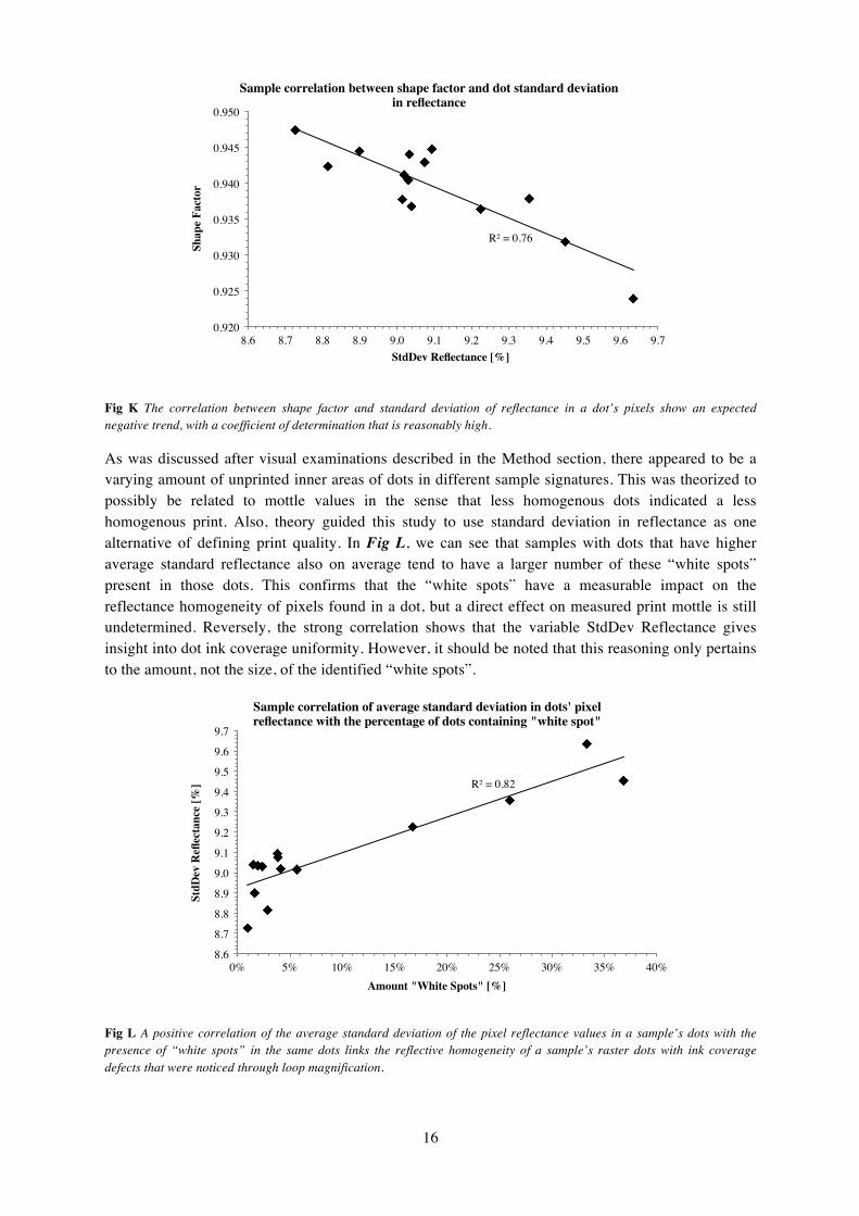
A suggested judgement of a sample’s print quality uses the combined variables of how round a dot is and how much its surface varies in reflectance. Fig K shows that for the analysed samples, the measured mean average shape factor correlates quite well with the mean average standard deviation of reflectance in a dot. A lower shape factor means a less circular dot, and a high standard deviation in reflectance for a dot means its pixels show a greater variation in their computed reflectance values.

R² = 0.83

15

16

17

18

19

20

21

22

23

24

25

17800 18000 18200 18400 18600 18800 19000 19200 19400 19600

Dot

gai

n [%

]

FilledArea [µm2]

Sample correlation between mean dot area and dot gain

16

Fig K The correlation between shape factor and standard deviation of reflectance in a dot’s pixels show an expected negative trend, with a coefficient of determination that is reasonably high.

As was discussed after visual examinations described in the Method section, there appeared to be a varying amount of unprinted inner areas of dots in different sample signatures. This was theorized to possibly be related to mottle values in the sense that less homogenous dots indicated a less homogenous print. Also, theory guided this study to use standard deviation in reflectance as one alternative of defining print quality. In Fig L, we can see that samples with dots that have higher average standard reflectance also on average tend to have a larger number of these “white spots” present in those dots. This confirms that the “white spots” have a measurable impact on the reflectance homogeneity of pixels found in a dot, but a direct effect on measured print mottle is still undetermined. Reversely, the strong correlation shows that the variable StdDev Reflectance gives insight into dot ink coverage uniformity. However, it should be noted that this reasoning only pertains to the amount, not the size, of the identified “white spots”.

Fig L A positive correlation of the average standard deviation of the pixel reflectance values in a sample’s dots with the presence of “white spots” in the same dots links the reflective homogeneity of a sample’s raster dots with ink coverage defects that were noticed through loop magnification.

R² = 0.76

0.920

0.925

0.930

0.935

0.940

0.945

0.950

8.6 8.7 8.8 8.9 9.0 9.1 9.2 9.3 9.4 9.5 9.6 9.7

Shap

e Fa

ctor

StdDev Reflectance [%]

Sample correlation between shape factor and dot standard deviation in reflectance

R² = 0.82

8.6

8.7

8.8

8.9

9.0

9.1

9.2

9.3

9.4

9.5

9.6

9.7

0% 5% 10% 15% 20% 25% 30% 35% 40%

StdD

ev R

eflec

tanc

e [%

]

Amount "White Spots" [%]

Sample correlation of average standard deviation in dots' pixel reflectance with the percentage of dots containing "white spot"

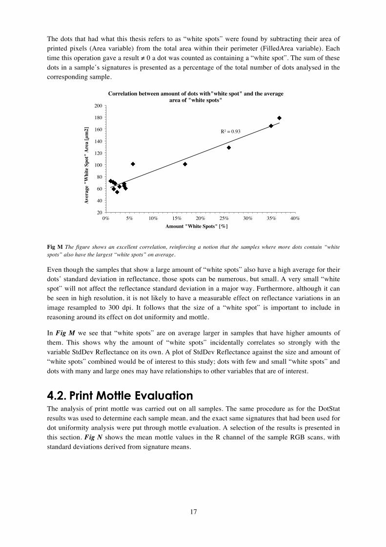
17

The dots that had what this thesis refers to as “white spots” were found by subtracting their area of printed pixels (Area variable) from the total area within their perimeter (FilledArea variable). Each time this operation gave a result ≠ 0 a dot was counted as containing a “white spot”. The sum of these dots in a sample’s signatures is presented as a percentage of the total number of dots analysed in the corresponding sample.

Fig M The figure shows an excellent correlation, reinforcing a notion that the samples where more dots contain “white spots” also have the largest “white spots” on average.

Even though the samples that show a large amount of “white spots” also have a high average for their dots’ standard deviation in reflectance, those spots can be numerous, but small. A very small “white spot” will not affect the reflectance standard deviation in a major way. Furthermore, although it can be seen in high resolution, it is not likely to have a measurable effect on reflectance variations in an image resampled to 300 dpi. It follows that the size of a “white spot” is important to include in reasoning around its effect on dot uniformity and mottle.

In Fig M we see that “white spots” are on average larger in samples that have higher amounts of them. This shows why the amount of “white spots” incidentally correlates so strongly with the variable StdDev Reflectance on its own. A plot of StdDev Reflectance against the size and amount of “white spots” combined would be of interest to this study; dots with few and small “white spots” and dots with many and large ones may have relationships to other variables that are of interest.

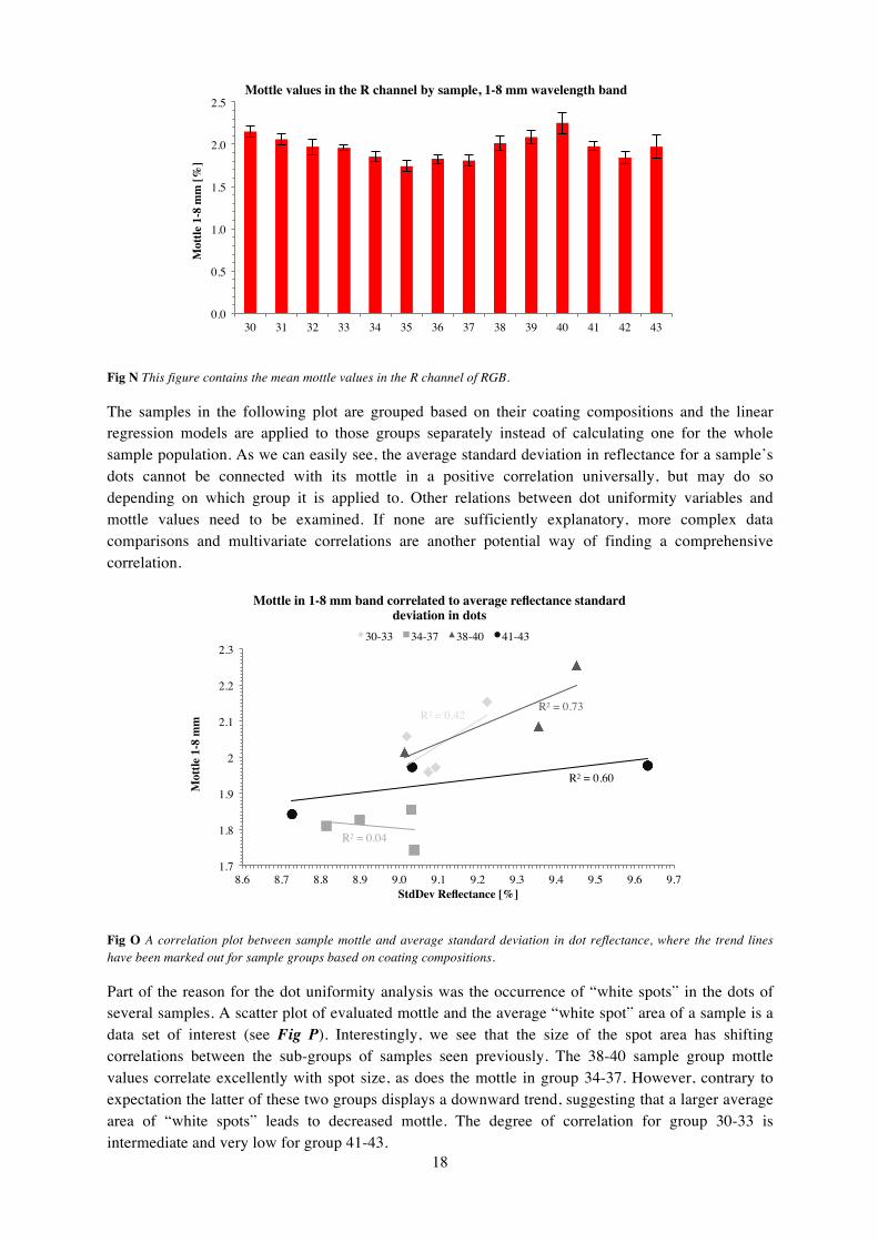
4.2. Print Mottle Evaluation The analysis of print mottle was carried out on all samples. The same procedure as for the DotStat results was used to determine each sample mean, and the exact same signatures that had been used for dot uniformity analysis were put through mottle evaluation. A selection of the results is presented in this section. Fig N shows the mean mottle values in the R channel of the sample RGB scans, with standard deviations derived from signature means.

R² = 0.93

20

40

60

80

100

120

140

160

180

200

0% 5% 10% 15% 20% 25% 30% 35% 40%

Aver

age

"Whi

te S

pot"

Are

a [µ

m2]

Amount "White Spots" [%]

Correlation between amount of dots with"white spot" and the average area of "white spots"

18

Fig N This figure contains the mean mottle values in the R channel of RGB.

The samples in the following plot are grouped based on their coating compositions and the linear regression models are applied to those groups separately instead of calculating one for the whole sample population. As we can easily see, the average standard deviation in reflectance for a sample’s dots cannot be connected with its mottle in a positive correlation universally, but may do so depending on which group it is applied to. Other relations between dot uniformity variables and mottle values need to be examined. If none are sufficiently explanatory, more complex data comparisons and multivariate correlations are another potential way of finding a comprehensive correlation.

Fig O A correlation plot between sample mottle and average standard deviation in dot reflectance, where the trend lines have been marked out for sample groups based on coating compositions.

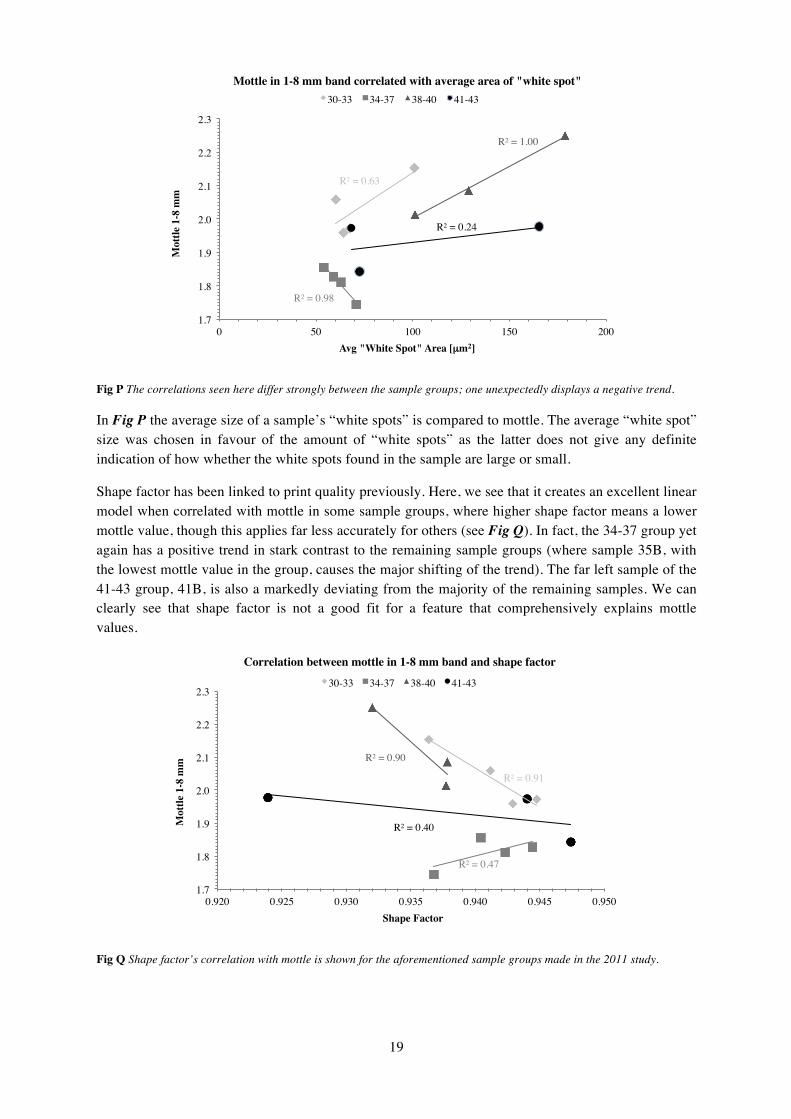
Part of the reason for the dot uniformity analysis was the occurrence of “white spots” in the dots of several samples. A scatter plot of evaluated mottle and the average “white spot” area of a sample is a data set of interest (see Fig P). Interestingly, we see that the size of the spot area has shifting correlations between the sub-groups of samples seen previously. The 38-40 sample group mottle values correlate excellently with spot size, as does the mottle in group 34-37. However, contrary to expectation the latter of these two groups displays a downward trend, suggesting that a larger average area of “white spots” leads to decreased mottle. The degree of correlation for group 30-33 is intermediate and very low for group 41-43.

0.0

0.5

1.0

1.5

2.0

2.5

30 31 32 33 34 35 36 37 38 39 40 41 42 43

Mot

tle 1

-8 m

m [%

]

Mottle values in the R channel by sample, 1-8 mm wavelength band

R² = 0.42

R² = 0.04

R² = 0.73

R² = 0.60

1.7

1.8

1.9

2

2.1

2.2

2.3

8.6 8.7 8.8 8.9 9.0 9.1 9.2 9.3 9.4 9.5 9.6 9.7

Mot

tle 1

-8 m

m

StdDev Reflectance [%]

Mottle in 1-8 mm band correlated to average reflectance standard deviation in dots

30-33 34-37 38-40 41-43

19

Fig P The correlations seen here differ strongly between the sample groups; one unexpectedly displays a negative trend.

In Fig P the average size of a sample’s “white spots” is compared to mottle. The average “white spot” size was chosen in favour of the amount of “white spots” as the latter does not give any definite indication of how whether the white spots found in the sample are large or small.

Shape factor has been linked to print quality previously. Here, we see that it creates an excellent linear model when correlated with mottle in some sample groups, where higher shape factor means a lower mottle value, though this applies far less accurately for others (see Fig Q). In fact, the 34-37 group yet again has a positive trend in stark contrast to the remaining sample groups (where sample 35B, with the lowest mottle value in the group, causes the major shifting of the trend). The far left sample of the 41-43 group, 41B, is also a markedly deviating from the majority of the remaining samples. We can clearly see that shape factor is not a good fit for a feature that comprehensively explains mottle values.

Fig Q Shape factor’s correlation with mottle is shown for the aforementioned sample groups made in the 2011 study.

R² = 0.63

R² = 0.98

R² = 1.00

R² = 0.24

1.7

1.8

1.9

2.0

2.1

2.2

2.3

0 50 100 150 200

Mot

tle 1

-8 m

m

Avg "White Spot" Area [µm2]

Mottle in 1-8 mm band correlated with average area of "white spot" 30-33 34-37 38-40 41-43

R² = 0.91

R² = 0.47

R² = 0.90

R² = 0.40

1.7

1.8

1.9

2.0

2.1

2.2

2.3

0.920 0.925 0.930 0.935 0.940 0.945 0.950

Mot

tle 1

-8 m

m

Shape Factor

Correlation between mottle in 1-8 mm band and shape factor

30-33 34-37 38-40 41-43

20

Shape factor is this study’s variable equivalent of “dot roundness” as it is described in the theory. The average shape factor for a sample’s dots does not necessarily say anything about mottle as a stand-alone variable, but it is still viable as indicative of better or worse print quality, especially in combination with other dot uniformity variables. For this reason, shape factor is appropriate to include in investigating multivariate relationships between mottle, shape factor and other relevant variables.

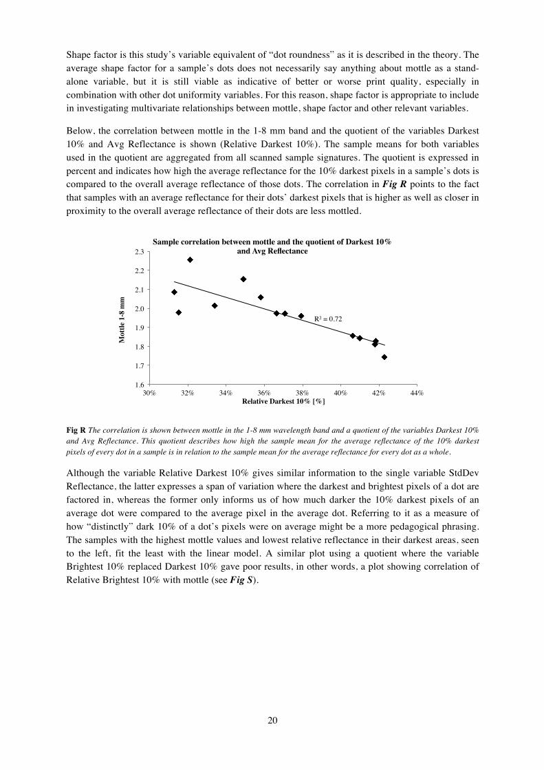
Below, the correlation between mottle in the 1-8 mm band and the quotient of the variables Darkest 10% and Avg Reflectance is shown (Relative Darkest 10%). The sample means for both variables used in the quotient are aggregated from all scanned sample signatures. The quotient is expressed in percent and indicates how high the average reflectance for the 10% darkest pixels in a sample’s dots is compared to the overall average reflectance of those dots. The correlation in Fig R points to the fact that samples with an average reflectance for their dots’ darkest pixels that is higher as well as closer in proximity to the overall average reflectance of their dots are less mottled.

Fig R The correlation is shown between mottle in the 1-8 mm wavelength band and a quotient of the variables Darkest 10% and Avg Reflectance. This quotient describes how high the sample mean for the average reflectance of the 10% darkest pixels of every dot in a sample is in relation to the sample mean for the average reflectance for every dot as a whole.

Although the variable Relative Darkest 10% gives similar information to the single variable StdDev Reflectance, the latter expresses a span of variation where the darkest and brightest pixels of a dot are factored in, whereas the former only informs us of how much darker the 10% darkest pixels of an average dot were compared to the average pixel in the average dot. Referring to it as a measure of how “distinctly” dark 10% of a dot’s pixels were on average might be a more pedagogical phrasing. The samples with the highest mottle values and lowest relative reflectance in their darkest areas, seen to the left, fit the least with the linear model. A similar plot using a quotient where the variable Brightest 10% replaced Darkest 10% gave poor results, in other words, a plot showing correlation of Relative Brightest 10% with mottle (see Fig S).

R² = 0.72

1.6

1.7

1.8

1.9

2.0

2.1

2.2

2.3

30% 32% 34% 36% 38% 40% 42% 44%

Mot

tle 1

-8 m

m

Relative Darkest 10% [%]

Sample correlation between mottle and the quotient of Darkest 10% and Avg Reflectance

21

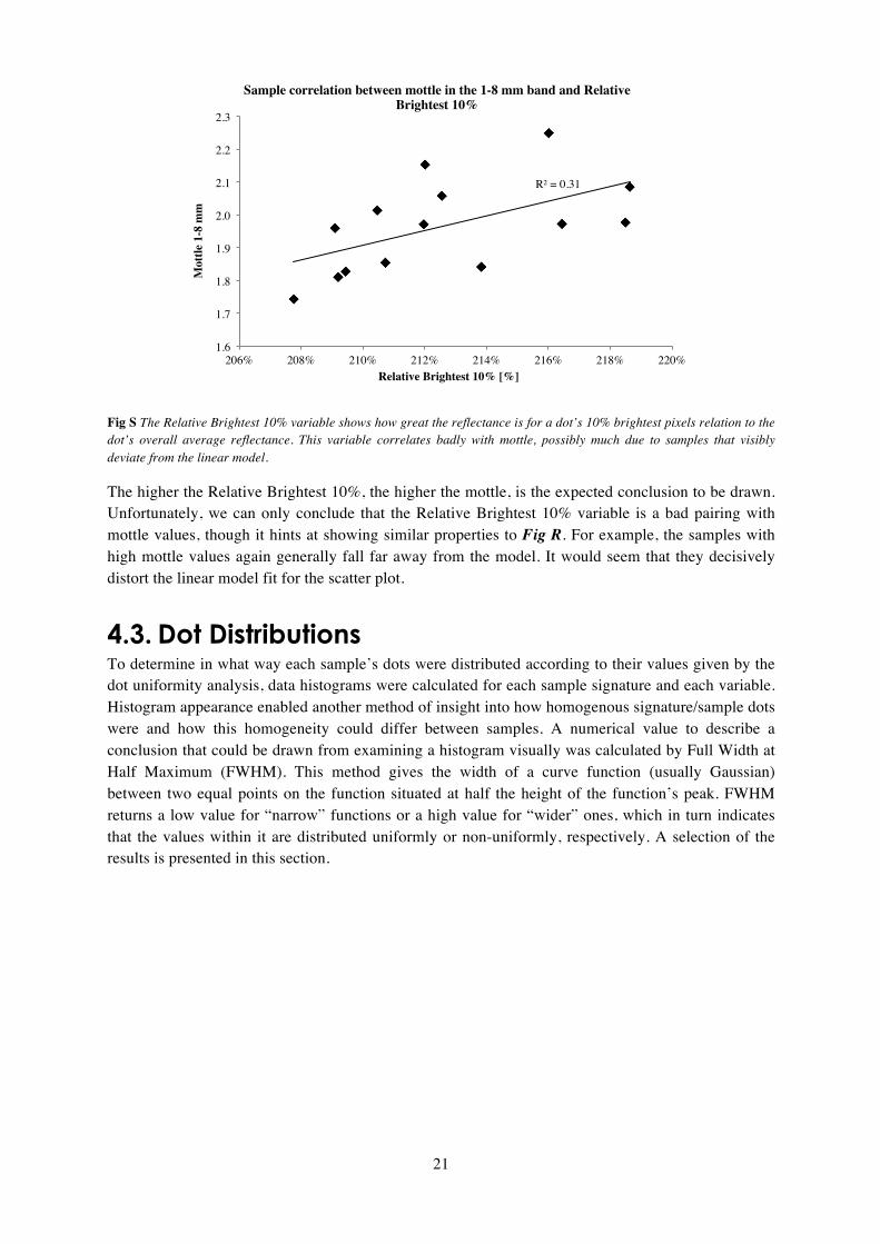
Fig S The Relative Brightest 10% variable shows how great the reflectance is for a dot’s 10% brightest pixels relation to the dot’s overall average reflectance. This variable correlates badly with mottle, possibly much due to samples that visibly deviate from the linear model.

The higher the Relative Brightest 10%, the higher the mottle, is the expected conclusion to be drawn. Unfortunately, we can only conclude that the Relative Brightest 10% variable is a bad pairing with mottle values, though it hints at showing similar properties to Fig R. For example, the samples with high mottle values again generally fall far away from the model. It would seem that they decisively distort the linear model fit for the scatter plot.

4.3. Dot Distributions To determine in what way each sample’s dots were distributed according to their values given by the dot uniformity analysis, data histograms were calculated for each sample signature and each variable. Histogram appearance enabled another method of insight into how homogenous signature/sample dots were and how this homogeneity could differ between samples. A numerical value to describe a conclusion that could be drawn from examining a histogram visually was calculated by Full Width at Half Maximum (FWHM). This method gives the width of a curve function (usually Gaussian) between two equal points on the function situated at half the height of the function’s peak. FWHM returns a low value for “narrow” functions or a high value for “wider” ones, which in turn indicates that the values within it are distributed uniformly or non-uniformly, respectively. A selection of the results is presented in this section.

R² = 0.31

1.6

1.7

1.8

1.9

2.0

2.1

2.2

2.3

206% 208% 210% 212% 214% 216% 218% 220%

Mot

tle 1

-8 m

m

Relative Brightest 10% [%]

Sample correlation between mottle in the 1-8 mm band and Relative Brightest 10%

22

Fig T This figure contains instances of histograms that display characteristics one can draw conclusions from by visual assessment. For example, it is evident that the histograms of signature 38B:5 and 40B:5 differ in width around their peaks, and consequently one has a more homogenously distributed dot population with regards to their standard deviation in reflectance. Such conclusions can arguably also be expressed in numerical terms.

Two conclusions can easily be drawn from a simple visual assessment of the above figure. Firstly, the histograms for these signatures differ in width around their peaks, even though their spans are very similar. Secondly, the values that their peaks correspond to on the x-axis vary. The first tells us how closely to the peak value (close to average) other dot values are located, the latter roughly tells where the signature average for the variable plotted against falls.

The FWHM values gathered were plotted against dot uniformity variables and mottle values. Fig U shows an instance of this, a correlation plot of sample means for StdDev Reflectance and FWHM StdDev Reflectance. Evidently, the samples with the highest average reflectance variation in their dots are also likely to have dots that vary the most amongst each other in regards to their reflectance variation. This is encouraging, since a sample can still be largely uniform overall even though its average StdDev Reflectance variable is high; the dots can simply be varying in reflectance at much the same level. Apparently, there is a good chance that this is more often false than true, although the FWHM of StdDev Reflectance should not be overlooked as a result.

Fig U The correlation here shows the relation between how greatly the reflectance in a sample’s dots varies on average and how strongly on average this variation varies between all the dots in the samples signatures.

0

50

100

150

200

250

300

7 7.5 8 8.5 9 9.5 10 10.5 11 11.5 12

Am

ount

of d

ots

Standard deviation in reflectance for dot

Distribution of dots according to their standard deviation in reflectance, 5th signatures of samples 38, 39 & 40

38B:5

39B:5

40B:5

R² = 0.87

8.6 8.7 8.8 8.9 9.0 9.1 9.2 9.3 9.4 9.5 9.6 9.7

0.8 0.9 1.0 1.1 1.2 1.3 1.4 1.5 1.6

StdD

ev R

eflec

tanc

e

FWHM StdDev Reflectance

Sample correlation of StdDev Reflectance in dots with FWHM StdDev Reflectance in dots

23

The average area of a sample’s “white spots” can be connected to how much the average reflectance of dots varies in a sample. The correlation between the two is fairly high, as can be seen in Fig V below. On the other hand, we still see the same clustering of samples with low average “white spot” areas that appears when this variable is used. As mentioned previously, this is may cause the fit of the data points to the linear model to be misleading, urging for caution in drawing any bolder conclusions about the result.

Fig V White spot area is related to how strongly the average reflectances of dots vary within a sample.

A sound expectation is that the varying distributions of dots according to their average reflectance should reasonably mirror the registered mottle values. In Fig W we would expect to see a dependable correlation between FWHM Avg Reflectance, which in a sense is the variable that most directly imitates a measurement of reflectance variation, and mottle in the 1-8 mm band.

Fig W The FWHM Avg Reflectance measurement gives an understanding of how much a sample’s dots vary in mean reflectance. Considering the theory discussed on mottle quantifies it as variations in reflectance, measured mottle should increase with higher FWHM Avg Reflectance.

R² = 0.73

1.5 1.6 1.7 1.8 1.9 2.0 2.1 2.2 2.3 2.4 2.5 2.6 2.7 2.8 2.9 3.0

0 50 100 150 200

FWH

M A

vg R

eflec

tanc

e

Avg "White Spot" Area [µm2]

Sample correlation between FWHM Avg Reflectance and the average areas of "white spots"

R² = 0.54

1.6

1.7

1.8

1.9

2.0

2.1

2.2

2.3

1.5 1.6 1.7 1.8 1.9 2.0 2.1 2.2 2.3 2.4 2.5 2.6 2.7 2.8 2.9 3.0

Mot

tle 1

-8 m

m

FWHM Avg Reflectance

Sample correlation of 1-8 mm mottle with FWHM Avg Reflectance

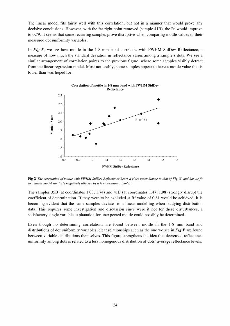
24

The linear model fits fairly well with this correlation, but not in a manner that would prove any decisive conclusions. However, with the far right point removed (sample 41B), the R2 would improve to 0,79. It seems that some recurring samples prove disruptive when comparing mottle values to their measured dot uniformity variables.

In Fig X, we see how mottle in the 1-8 mm band correlates with FWHM StdDev Reflectance, a measure of how much the standard deviation in reflectance varies among a sample’s dots. We see a similar arrangement of correlation points to the previous figure, where some samples visibly detract from the linear regression model. Most noticeably, some samples appear to have a mottle value that is lower than was hoped for.

Fig X The correlation of mottle with FWHM StdDev Reflectance bears a close resemblance to that of Fig W, and has its fit to a linear model similarly negatively affected by a few deviating samples.

The samples 35B (at coordinates 1.03, 1.74) and 41B (at coordinates 1.47, 1.98) strongly disrupt the coefficient of determination. If they were to be excluded, a R2 value of 0,81 would be achieved. It is becoming evident that the same samples deviate from linear modelling when studying distribution data. This requires some investigation and discussion since were it not for these disturbances, a satisfactory single variable explanation for unexpected mottle could possibly be determined.

Even though no determining correlations are found between mottle in the 1-8 mm band and distributions of dot uniformity variables, clear relationships such as the one we see in Fig Y are found between variable distributions themselves. This figure strengthens the idea that decreased reflectance uniformity among dots is related to a less homogenous distribution of dots’ average reflectance levels.

R² = 0.54

1.6

1.7

1.8

1.9

2.0

2.1

2.2

2.3

0.8 0.9 1.0 1.1 1.2 1.3 1.4 1.5 1.6

Mot

tle 1

-8 m

m

FWHM StdDev Reflectance

Correlation of mottle in 1-8 mm band with FWHM StdDev Reflectance

25

Fig Y Among samples, the variation in reflectance standard deviation among dots correlates quite highly with the variation of the average reflectance of those dots.

Sadly, neither of these factors correlates sufficiently well with 1-8 mm band mottle by themselves.

4.4. Multiple Linear Regression Analysis Only using simple linear regression may not always be enough to illustrate how a group of variables relate to each other. A data set consists of points of correlation between the variables 𝑋 and 𝑌. Simple linear regression finds a model in the form of a straight line that gives the smallest possible sum of the vertical distances from the points in the data set to that line. In a simple linear regression model, a single measurement 𝑌 can only be related to a single predictor  𝑋. The coefficient of determination R2 varies between 0 and 1 and is interpreted as an expression of how well a data set’s points fit to the linear model, where 1 indicates perfect fit. However, using multiple linear regression (MLR) allows us to determine how well the relationship between several predictors 𝑋!,𝑋!,… ,𝑋! and a response measurement 𝑌 fit to a linear model. MLR is necessary to explore more advanced correlations between dot uniformity variables and evaluated mottle.

The MLR analysis produces regression coefficients 𝛽 for each predictor 𝑋, and the intercept 𝛼. The MLR model is written on the form:

𝑌! = 𝛼 + 𝛽!𝑋!,! +⋯+ 𝛽!𝑋!,!

Where 𝑋!,! denotes the 𝑛!! predictor variable measured at the 𝑖!! observation for 𝑖 = 1,2,… , 𝑛. The values given by the MLR model at every observation 𝑖 (sample) are plotted against the original measurement 𝑌 and R2 is then calculated for their fit to a linear model. A selection of the results is presented in this section.

In this first figure, a strong correlation between the variable StdDev reflectance and the amount of dots in a sample containing a “white spot” is noted (see Fig Z), but data on the average area of “white spots” in samples has also been factored into the plot, using MLR calculations. The below result further establishes that StdDev Reflectance has a clear connection to white spot occurrence and size.

R² = 0.81

1.5

1.7

1.9

2.1

2.3

2.5

2.7

2.9

3.1

0.8 0.9 1.0 1.1 1.2 1.3 1.4 1.5 1.6

FWH

M A

vg R

eflec

tanc

e

FWHM StdDev Reflectance

Sample correlation of FWHM StdDev Reflectance with FWHM Avg Reflectance

26

Fig Z Here 𝑌! is based on values Amount “White Spots” and Avg "White Spot" Area.

Further use of MLR models supplies evidence for what variables could be used to predict reflectance variations among dots (see Fig AA). A high fit to a linear model was calculated using StdDev Reflectance, average “white spot” area and the quotient of the Darkest 10% and Avg Reflectance variables (Relative Darkest 10%) as predictors in the MLR model equation. Despite the increased complexity of relations among these data, we may deduce that some aspects of dot uniformity, when combined, are correlated well with how varyingly dark or bright halftone dots become in a halftone. On the other hand, some reserve in drawing conclusions should be practiced, since the majority of samples have low mean StdDev Reflectance values compared to a few others. They are clustered to the left and the actual linearity in this plot is potentially deceiving.

Fig AA A Correlation diagram between FWHM Reflectance and 𝑌 values gained from MLR combination of three different data gained from dot uniformity analysis: StdDev Reflectance, average “white spot” area and the quotient of the variables Darkest 10% and Avg Reflectance.

R² = 0.83

8.6

8.7

8.8

8.9

9.0

9.1

9.2

9.3

9.4

9.5

9.6

9.7

8.6 8.7 8.8 8.9 9.0 9.1 9.2 9.3 9.4 9.5 9.6 9.7

StdD

ev R

eflec

tanc

e

𝑌𝑖 = 9,03 + 2,33 × 𝑋𝑖,1 − 0,0019 × 𝑋𝑖,2

Sample correlation between average StdDev Reflectance and MLR model values using amount of dots with "white spots" and the average

area of those spots

R² = 0.85

1.5

2.0

2.5

3.0

1.5 2.0 2.5 3.0

FWH

M A

vg R

eflec

tanc

e

𝑌𝑖 = 2,56 + 0,0033 × 𝑋𝑖,1 + 0,12 × 𝑋𝑖,2 − 4,79 × 𝑋𝑖,3

Sample correlation between FWHM Reflectance and MLR model values using three data types from dot uniformity analysis

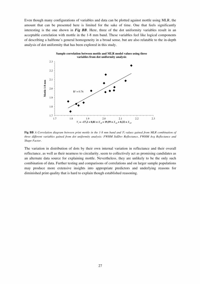
27

Even though many configurations of variables and data can be plotted against mottle using MLR, the amount that can be presented here is limited for the sake of time. One that feels significantly interesting is the one shown in Fig BB. Here, three of the dot uniformity variables result in an acceptable correlation with mottle in the 1-8 mm band. These variables feel like logical components of describing a halftone’s general homogeneity in a broad sense, but are also relatable to the in-depth analysis of dot uniformity that has been explored in this study.

Fig BB A Correlation diagram between print mottle in the 1-8 mm band and 𝑌𝑖 values gained from MLR combination of three different variables gained from dot uniformity analysis: FWHM StdDev Reflectance, FWHM Avg Reflectance and Shape Factor.

The variation in distribution of dots by their own internal variation in reflectance and their overall reflectance, as well as their nearness to circularity, seem to collectively act as promising candidates as an alternate data source for explaining mottle. Nevertheless, they are unlikely to be the only such combination of data. Further testing and comparisons of correlations and on larger sample populations may produce more extensive insights into appropriate predictors and underlying reasons for diminished print quality that is hard to explain though established reasoning.

R² = 0.76

1.7

1.8

1.9

2.0

2.1

2.2

2.3

1.7 1.8 1.9 2.0 2.1 2.2 2.3

Mot

tle 1

-8 m

m

𝑌𝑖 = −17,2 + 0,81 × 𝑋𝑖,1 + 19,59 × 𝑋𝑖,2 + 0,32 × 𝑋𝑖,3

Sample correlation between mottle and MLR model values using three variables from dot uniformity analysis

28

5. Discussion Even though the data collected while working with this thesis is extensive, perhaps there is value in it that has not been researched. For example, the potential affiliations of ink absorption (i.e. due to modified coating content) and white-top mottle with variables measured in the dot uniformity analysis have been left uninspected. Ink absorption and coating structure may quite possibly affect the way that a printed dot is impressed on the substrate in ways that are relevant to this thesis. White-top mottle is already known to weigh in to the results of mottle evaluation using STFI-Mottle.

There is an obvious complication with only using information from the pixels in the R channel when conducting mottle evaluation, as mottling that occurs outside of the areas with printed ink is likely to be discarded or improperly calculated. For example, unprinted substrate in a scanned image also contains R channel pixels (a problem handled in dot uniformity analysis by using histograms and thresholding), but consists of numerous pixels in the G and B channel as well. Granted, the mottle evaluation does make use of the surface of the substrate even when limited to the R channel, but it will be perceived as more homogenously white. This means that the inherent mottle in the white coating of the printed substrate, white-top mottle, is at least partially excluded from analysis.

In short, the limited knowledge of the detailed functioning of the scanner that was used in place of a much more familiar one was a trade-off. The study benefited from the improved optics and reproduction of detail at higher resolutions, but suffered from the lack of operating knowledge. This downside was most clearly represented in the markedly different pixel distributions for each RGB channel of the scanned images. It is likely that some information and image detail was lost due to peaking G and B histograms, and these defects were caused by adjusting scanner settings. On the other hand, these adjustments were necessary to reproduce a scan of material needed for calibration that would be accepted by analysis software. Additionally, a parallel goal was for the scanning to produce images with a detailed R histogram, which those adjusted settings also facilitated for all samples.

The reason behind calculating mottle as reflectance variations in grayscale over all three RGB channels after converting is that it has been proven to correspond well with the opinion of human test subjects. The same research has not been done for mottle values from solely the R channel, so it is difficult to say anything about the discrepancies its use has led to. It should be taken into consideration that the internal ranking amongst the samples used was not drastically different between mottle values from the R channel calculated in 2014 and the ones calculated for the Innventia Report in 2011. Given more time, this would have been an interesting addition to the results of this thesis.

The use of the DotStat software was new and untested in this context. Although it appeared successful in identifying dots in general, it may need more development to identify so-called “white spots”, for example. The thresholding method used in DotStat could be modified and tested for better results in this matter, it was evident that it could not always distinguish effectively between printed and unprinted area as accurately as a visual examination of the scanned images it processed. Therefore, it is suspected that measurements regarding the existence and size of “white spots” could have been distorted. However, the actual effect of erroneous pixel sorting on such data is unknown.

The intention of using MLR analysis was to find multivariate relationships between variables measured in this study and evaluated print mottle. Though correlations could be found between single variables and mottle, none of these could be put forward as a fully explanatory of the mottle values registered. On the other hand, the fit of points of two correlating data variables to a linear model for

29

the whole sample population would occasionally be shifted to an inadequate level by one or few samples. So, at times a suggestion of a well-distributed linearity could be discerned in some figures while excluding “disruptive “samples, despite the R2 value being too low. Consider the case of Fig R, for instance, where the leftmost samples gradually detract more from the linear model the higher their x-value, in contrast to the remaining samples, which are showing an excellent fit.

When it comes to employing MLR to find meaningful data correlations between dot uniformity variables and mottle values, there is a great amount of combinations that predictors can be placed in to produce various models. A suggestion is that any further analysis should include complementary examination of results using MLR. Furthermore, this could be done in combination with including an extended selection of factors of interest in explaining print mottle.

Previously, the samples were divided into groups based on the compositions of their coating. These groups have largely been disregarded in this study as the hope was to find one variable or a combination of variables that could display a clear-cut relation to print mottle for all the samples collectively. Studying the data gained in this thesis and how it relates to mottle in these or other sample sub-groups may offer a valuable added perspective on the varying effects that the dot uniformity variables that have been mentioned have on mottle.

There is strong evidence in this study’s results that the appearance and size of “white spots” is related to the values of other variables. These variables have been difficult to link directly to mottle value variations in the 1-8 mm bands, but this does not exclude the possibility that reflectance variations in shorter wavelength bands have been affected in a different manner. Samples that deviated strongly in what could otherwise be assessed as quite linear correlations disrupted the results in a way that made comprehensive conclusions problematic. Upon further examination, the source of these deviations appears to be an unexpected difference in mottle amount between wavelength bands in certain samples.

The DotStat analysis registers reflectance values on a pixel level in high-resolution images. The calculations that follow are therefore first and foremost returning data that represents small scale features or variations. No measurement or analysis is actually performed on a larger scale or in lower resolution images, except for the mottle evaluation – pixel level data is still being used in, for instance, dot distribution calculations. Therefore, the DotStat results can be directly related to the short wavelength mottle values, but at the same time not reflect the amount of mottle in longer wavelength bands. Certain samples display a different ranking among the sample group when it comes to shorter wavelength mottle than when they are ranked according to mottle in the 1-8 mm wavelength band.

A quick investigation indicates that some of the repeatedly deviating samples have a high mottle in shorter wavelengths and low mottle in longer wavelengths, compared to other samples. These samples also have high values for dot uniformity variables that correlate better with mottle in the 1-8 mm band for other samples. In other words, where a high dot uniformity variable value is expected to coincide with a high value in 1-8 mm band mottle, those samples do not fulfill that expectation. On the other hand, the very same dot uniformity variable data gathered from them seems to be more representative of their mottle values in shorter wavelength bands. A more thorough investigation of the correlation between dot uniformity variables and short wavelength mottle is recommended.

30

6. Conclusion A method was devised for scanning high-resolution images of halftone raster dots printed with cyan ink in order to analyse a number of their properties with highest possible detail. By employing thresholding of the scanned images, a separation of printed dots from unprinted substrate was successfully made. Consequently, measurements of both the dots’ geometry and reflectance characteristics were made. Later, a mottle evaluation using the same scanned material was done using STFI-Mottle.

The “white spots” in the halftones were identified as possible causes or predictors of halftone print mottle early on in the thesis process. They were identified using thresholding in image analysis software. The threshold calculation had to be altered in order to make those findings more distinct, as it became clear that they were being omitted with the default method. As a result actual area deficiencies for identified dots could be measured more explicitly for every identified dot. The degree to which “white spots” appeared as well as their average area in samples could be linked to the values of variables from dot uniformity analysis. The mean standard deviation in reflectance in the samples’ dots was well correlated with data gathered on “white spots”, as was the variation in average reflectance between dots in samples.

The mean dot area that was measured correlated well with previously measured dot gain, for all samples. The mean standard deviation of reflectance in dots correlated well with measured shape factor, indicating that a less circular dot also may suffer from less consistently transferred ink. Additionally, the mean standard deviation in reflectance in dots was generally higher in samples with a greater number of dots containing “white spots”. Furthermore, to settle any reservations about proportionality between the amount of “white spots” and their size in samples, it was shown that the correlation between these measurements in a scatter plot resulted in a linear model with a coefficient of determination of 0.93.

A new mottle evaluation was carried out with the aim of being more consistent with the method used for dot uniformity analysis than the evaluation of mottle done previously. Focus was directed at the 1-8 mm band of mottle measured in the R channel of RGB sample scans. The mean standard deviation in reflectance of dots was found to not offer a comprehensive correlation with print mottle, even though it did correlate to a varying degree with various groupings of the samples. The same can be said for the average area of “white spots” in a sample, but here the correlations resulted in even more juxtaposed trends. Unexpectedly, the group with coating containing clay additives had higher mottle where the average area of the “white spots” was lower.

It was also shown that average dot roundness could not comprehensively account for the variations of the samples’ mottle values; group 34-37 once more had an opposite trend compared to remaining samples. The degree to which the mean reflectance of a dot’s 10% darkest pixels is darker than the dot’s overall mean reflectance, on average, can be expressed by the quotient of the variables Darkest 10% and Avg Reflectance, or Relative Darkest 10%. This quotient showed a more promising direct correlation with print mottle than any other single variable, and its implications ought to be investigated further.

Histograms were calculated in order to examine the distributions of dots in samples according to the variables measured in the dot uniformity analysis. FWHM was used to numerically describe these distributions; a higher FWHM value equalled a less homogenous distribution of dots. It was shown that samples with a high mean standard deviation in reflectance in their dots also had a higher

31

variation of standard deviation in reflectance between dots. The average area of “white spots” in a sample seemed to affect the variation of average reflectance among its dots. The variation of average reflectance among a sample’s dots, in turn, did not prove to be a very dependable predictor of print mottle, despite it bearing a rough resemblance to how mottle is defined in theory.

MLR analysis was used to investigate whether using a combination of dot uniformity variables as predictors could act as a more robust expression of print mottle, amongst other things. The number of dots with “white spots” in a sample, in combination with the average area of those spots, correlate well with a sample’s mean standard deviation in reflectance for its dots. The variations of average reflectance among dots in a sample are very well correlated with a combination of that sample’s average standard deviation in reflectance of dots, average “white spot” area as well as the quotient of its Darkest 10% and Avg Reflectance values. Many possibilities still remain, but one suggestion of expressing print mottle facilitated by MLR was presented. Using a sample’s mean dot roundness as well as variation in average reflectance and standard deviation in reflectance among its dots comprises an adequate, though not complete, idea of explaining print mottle.

32

7. Application The aim of this thesis is to expand the knowledge base of the causes of mottle, specifically in flexographic printing but possibly in other printing techniques as well. Defects that affect print quality are well known and can be described and assessed visually, print mottle is one of those defects. Even though print mottle has itself been quantified in the methodology used by Innventia AB, and the know-how on its origins is substantial, it may not always be sufficient to determine quality as a numerical value by itself.

This thesis has investigated alternate ways of explaining the occurrence of mottle in halftone samples where traditional reasoning has been insufficient. The idea has been to extensively analyse the uniformity of the samples’ raster dots, by quantifying that concept into several variables based on reflectance and geometrical calculations. Included in this work is the development of a previously untested methodology of gathering raw data by software analysis. Although the intention was to find reasons for unexpected mottle levels, the data gathered in this thesis also provides an exploration into new possibilities of defining and quantifying print quality in general. The method used to extract this data can be applied and repeated at Innventia AB in the future, ensuring its development and refining if the results are deemed useful.

The new data variables that describe dot uniformity can to some extent be related to print mottle, but are in no way limited to that relationship. In fact, the need for new objective measurement of print quality is still great, and further research into the implications of the dot uniformity data may yield results that are of interest on an industrial scale. Dot uniformity has been somewhat investigated in other print techniques, but not using the same amount of data variables as in this thesis, meaning that this specific field of research is still largely unexplored. The methodology developed should be applied on additional halftones. Furthermore, examining how the dot uniformity variables are related to substrate topography, coating composition and other material properties may be the next phase of research. There is clear potential and use for gathering this type of data on halftone production, as there are additional quality aspects apart from mottle that could possibly be defined numerically using extensive dot uniformity data. In conclusion, the knowledge on flexographic print dot features gained during in thesis may serve as a valuable base for further research into quantifying print quality.

33

8. Resources Christofferson, J., 2004. Evaluation of Systematic & Colour Print Mottle. MSc. Linköping University

Fahlcrantz, C-M., 2005. On the Evaluation of Print Mottle. Doctoral Thesis. Royal Institute of Technology.

Fleming, P D., Cawthorne, J E., Mehta, F., Halwawala, S. and Joyce, M K., 2003. Interpretation of Dot Fidelity of Ink Jet Dots Based on Image Analysis. The Journal of Imaging Science and Technology, 47(5), pp. 394-399.

Habekost, M. & Atkinsons, R., 2013. Improving the Assessment of Geometrical Print Image Fidelity. In: IARIGAI, 40th International Research Conference of iarigai. Chemnitz, Germany, September 2013. Darmstadt: iarigai.

Johansson, K., Lundberg, P. and Ryberg R., 2008. Grafisk Kokbok, 3rd ed. Malmö: Arena.

Johansson, P-Å., 1993. Print Mottle Evaluation by Band-Pass Image Analysis. Advances in Printing Science and Technology, 22, p. 403.

Johansson, P-Å., 1999. Optical Homogeneity of Prints. Doctoral Thesis. Royal Institute of Technology.

Madstedt, S., 2008. The Impact of Coating Composition on Print Mottle and Print Gloss Variations in Sheet-Fed Offset. MSc. Royal Insititute of Tecnology.

Namedanian, M., 2013. Characterization of Halftone Prints based on Microscale Image Analysis. Doctoral Thesis. Linköping University.

Ragnarsson, M., 2012. Variations Related to Print Mottle in Starch-Containing Paper Coatings. Doctoral Thesis. Karlstad University.

Sonmez, S., Fleming, P D., Joyce, M K., & Ozden, O., 2010. Effects of Coat Weight and Pigment Selection on Flexographic Printability of Coated Test Liners. In: PaperCon 2010 Conference.

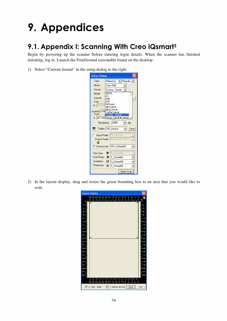
34

9. Appendices

9.1. Appendix I: Scanning With Creo iQsmart3 Begin by powering up the scanner before entering login details. When the scanner has finished initiating, log in. Launch the ForeGround executable found on the desktop.

1) Select “Custom format” in the setup dialog to the right.

2) In the layout display, drag and resize the green bounding box to an area that you would like to scan.

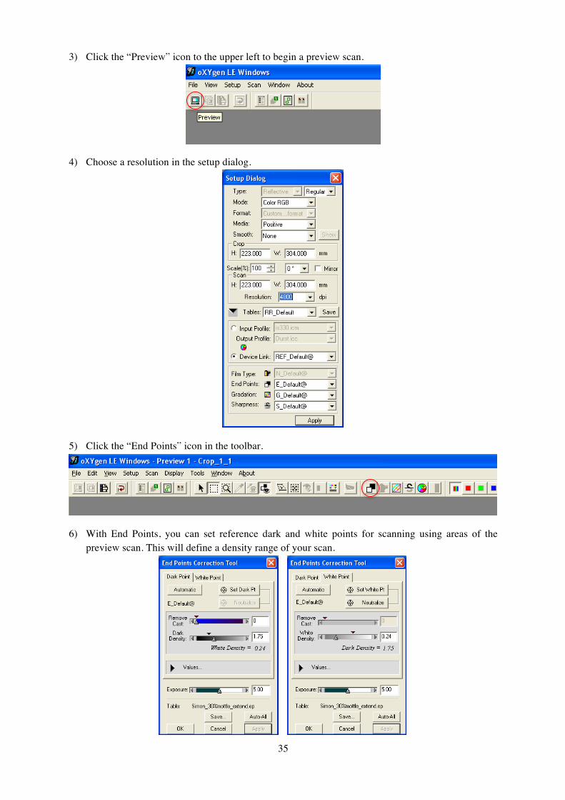
35

3) Click the “Preview” icon to the upper left to begin a preview scan.

4) Choose a resolution in the setup dialog.

5) Click the “End Points” icon in the toolbar.

6) With End Points, you can set reference dark and white points for scanning using areas of the preview scan. This will define a density range of your scan.

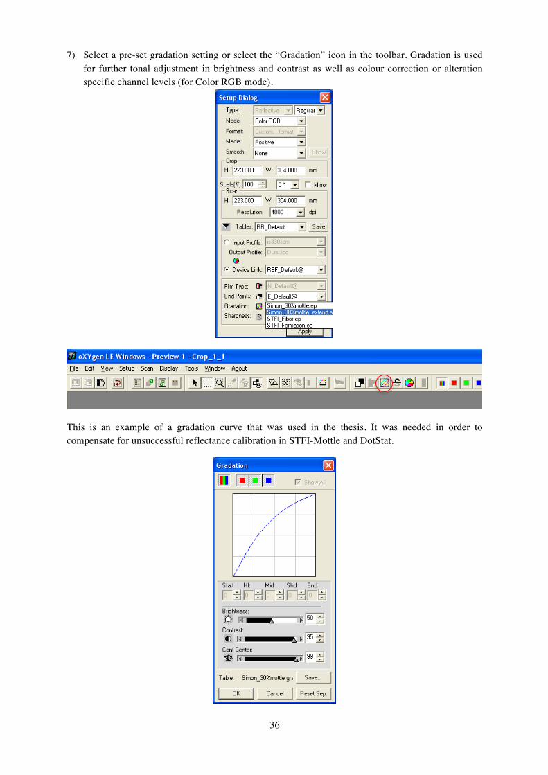
36

7) Select a pre-set gradation setting or select the “Gradation” icon in the toolbar. Gradation is used for further tonal adjustment in brightness and contrast as well as colour correction or alteration specific channel levels (for Color RGB mode).

This is an example of a gradation curve that was used in the thesis. It was needed in order to compensate for unsuccessful reflectance calibration in STFI-Mottle and DotStat.

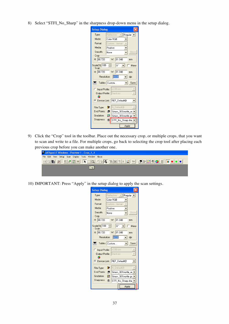
37

8) Select “STFI_No_Sharp” in the sharpness drop-down menu in the setup dialog.

9) Click the “Crop” tool in the toolbar. Place out the necessary crop, or multiple crops, that you want to scan and write to a file. For multiple crops, go back to selecting the crop tool after placing each previous crop before you can make another one.

10) IMPORTANT: Press “Apply” in the setup dialog to apply the scan settings.

38

11) Press “Scan” in the toolbar. Hold Ctrl before pressing to scan multiple crops if you have drawn more than one.

12) Write the files to the “SATA 300 GB” disk. Remember to change the file format to .tif and write a file name, then press “Save”. If you are scanning multiple crops, you will have to rename each consecutive file and press “Save” each time.

9.2. Appendix II: DotStat Analysis DotStat requires some basic knowledge to operate correctly. This appendix assumes that the user is familiar with the use of reflectance calibration frames in STFI-Mottle and how what requirements they need to fulfil. When analysing scans using DotStat, the image format must be .tif.

1) Begin by pressing “Load TIFF”. You will be prompted to select an image. Click “Open”.

39

2) Let DotStat load the image. When it is finished it will display “TIFF loaded!” below. Press “Select ROI” and draw a bounding box in the image that will determine a region of interest (ROI). Make sure the ROI that you draw is within the boundaries of the image. When the ROI is set, reflectance calibration will be performed using an image histogram.

3) Click “Find threshold” for DotStat to automatically detect a suitable threshold using an image histogram. The threshold will be calculated and updated. The number in this field can also be changed manually, either to a fixed value or by calculating a percentage for each image using the automatically generated value. Double the automatically identified threshold value and multiply by 0.45 to get the threshold located 45% of the way between histogram peaks, for instance.

40

4) Name the file in “Result file” and enter a comment that will be included in the file, if needed. Check “Plot all steps” to receive figures for every step of calculations and conversions made. Check “Plot histograms” to see histograms for each dot object with regards to the dot uniformity variables. Check “Remove dirt” for automated removal of dirt and other small scale defects (unwanted pixels). Press “Analyze” when ready, the file will be saved in .xl format, in the “Results” folder of the DotStat directory.

9.3. Appendix III: Full Width at Half Maximum The following illustration depicts how FWHM is measured in a histogram, for easier understanding. A maximum value is located in the graph. There are two points located on the graph where the y-value corresponds to half of the y maximum. The distance along the x-axis between those points is given as the FWHM value.

41

9.4. Appendix IV: MLR Analysis Progression This is an example of how MLR was applied in examining possible favourable multivariate correlations between mottle and relevant variables gathered in dot uniformity analysis. Variables were added in succession with the aim of improving the multivariate correlation R2, which is marked in green below. Variables were chosen based on their relevance to existing mottle definition and their assessed effect on dot uniformity.