Degree growth of matrix inversion: Birational maps of symmetric, cyclic matrices

November 19, 2005

Degree Growth of Matrix Inversion:Birational Maps of Symmetric, Cyclic Matrices

Eric Bedford and Kyounghee Kim

§0. IntroductionLet Mq denote the space of q×q matrices, and let P(Mq) denote its projectivization. For

a matrix x = (xij) we consider two maps. One is J(x) = (x−1ij ) which takes the reciprocal of

each entry of the matrix, and the other is the matrix inverse I(x) = (xij)−1. The involutions

I and J , and thus the mapping K = I J , arise as basic symmetries in Lattice StatisticalMechanics (see [BM], [BMV]). This leads to the problem of determining the iterated behaviorof K on P(Mq) (see [AABHM], [AABM], [AMV2], [BV]). A basic question is to know thedegree complexity

δ(K) := limn→∞

(deg(Kn))1/n = limn→∞

(deg(K · · · K))1/n

of the iterates of this map. (The quantity log δ is also called the algebraic entropy in the paper[BV].)

The q×q matrices correspond to the coupling constants of a system in which each locationhas q possible states. In more specific models, there may be additional symmetries, and suchsymmetries define a K-invariant subspace S ⊂ P(Mq) (see [AMV1]). In general, the degreeof the restriction K|S will be lower than the degree of K, and the corresponding question inthis case is to know δ(K|S) = limn→∞(deg(Kn|S))1/n. An example of this, related to Pottsmodels, is the subspace Cq of cyclic matrices, i.e., matrices (xij) for which xij depends only onj − i (mod q). A cyclic matrix is thus determined by numbers x0, . . . , xq−1 according to theformula

M(x0, . . . , xq−1) =

x0 x1 xq−1

xq−1. . .

. . .

. . .. . . x1

x1 xq−1 x0

. (0.1)

The degree growth of K|Cq was determined in [BV]. Another case of evident importance isSCq, the symmetric, cyclic matrices. The degree growth of K|SCq was determined in [AMV2]for prime q. In this paper we determine δ(K|SCq) for all q. In doing this, we expose a generalmethod of determining δ, which we believe will also be applicable to the study of δ(K|S) formore general spaces S.

The mappings K|Cq and K|SCq lead to maps of the form f = L J on PN , where L islinear, and J = [x−1

0 : · · · : x−1N ]. In the case of K|Cq, L = F is the matrix representation of

the finite Fourier transform, and the entries are qth roots of unity. By the internal symmetryof the map, the exceptional hypersurfaces Σi = xi = 0 all behave in the same way, and δfor these maps is found easily by the method of regularization described below. The family of“Noetherian maps” was introduced in [BHM] and generalized to “elementary maps” in [BK1].These maps have the feature that all exceptional hypersurfaces behave like

Σi → ∗ → · · · → ei Vi, (0.2)

1

November 19, 2005

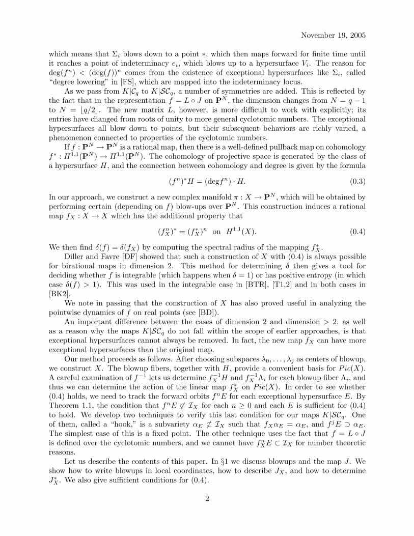
which means that Σi blows down to a point ∗, which then maps forward for finite time untilit reaches a point of indeterminacy ei, which blows up to a hypersurface Vi. The reason fordeg(fn) < (deg(f))n comes from the existence of exceptional hypersurfaces like Σi, called“degree lowering” in [FS], which are mapped into the indeterminacy locus.

As we pass from K|Cq to K|SCq, a number of symmetries are added. This is reflected bythe fact that in the representation f = L J on PN , the dimension changes from N = q − 1to N = ⌊q/2⌋. The new matrix L, however, is more difficult to work with explicitly; itsentries have changed from roots of unity to more general cyclotomic numbers. The exceptionalhypersurfaces all blow down to points, but their subsequent behaviors are richly varied, aphenomenon connected to properties of the cyclotomic numbers.

If f : PN → PN is a rational map, then there is a well-defined pullback map on cohomologyf∗ : H1,1(PN ) → H1,1(PN ). The cohomology of projective space is generated by the class ofa hypersurface H, and the connection between cohomology and degree is given by the formula

(fn)∗H = (degfn) · H. (0.3)

In our approach, we construct a new complex manifold π : X → PN , which will be obtained byperforming certain (depending on f) blow-ups over PN . This construction induces a rationalmap fX : X → X which has the additional property that

(fnX)∗ = (f∗

X)n on H1,1(X). (0.4)

We then find δ(f) = δ(fX) by computing the spectral radius of the mapping f∗X .

Diller and Favre [DF] showed that such a construction of X with (0.4) is always possiblefor birational maps in dimension 2. This method for determining δ then gives a tool fordeciding whether f is integrable (which happens when δ = 1) or has positive entropy (in whichcase δ(f) > 1). This was used in the integrable case in [BTR], [T1,2] and in both cases in[BK2].

We note in passing that the construction of X has also proved useful in analyzing thepointwise dynamics of f on real points (see [BD]).

An important difference between the cases of dimension 2 and dimension > 2, as wellas a reason why the maps K|SCq do not fall within the scope of earlier approaches, is thatexceptional hypersurfaces cannot always be removed. In fact, the new map fX can have moreexceptional hypersurfaces than the original map.

Our method proceeds as follows. After choosing subspaces λ0, . . . , λj as centers of blowup,we construct X. The blowup fibers, together with H, provide a convenient basis for Pic(X).A careful examination of f−1 lets us determine f−1

X H and f−1X Λi for each blowup fiber Λi, and

thus we can determine the action of the linear map f∗X on Pic(X). In order to see whether

(0.4) holds, we need to track the forward orbits fnE for each exceptional hypersurface E. ByTheorem 1.1, the condition that fnE 6⊂ IX for each n ≥ 0 and each E is sufficient for (0.4)to hold. We develop two techniques to verify this last condition for our maps K|SCq. Oneof them, called a “hook,” is a subvariety αE 6⊂ IX such that fXαE = αE, and f jE ⊃ αE.The simplest case of this is a fixed point. The other technique uses the fact that f = L Jis defined over the cyclotomic numbers, and we cannot have fn

XE ⊂ IX for number theoreticreasons.

Let us describe the contents of this paper. In §1 we discuss blowups and the map J . Weshow how to write blowups in local coordinates, how to describe JX , and how to determineJ∗

X . We also give sufficient conditions for (0.4).

2

November 19, 2005

In §2, we show how this approach may be applied to K|Cq. In this case, the exceptionalorbits are of the form (0.2). We construct the space X by blowing up the points of theexceptional orbits. After these blowups, the induced map fX has no exceptional hypersurfaces,which implies that (0.4) holds. A calculation of f∗

X and its spectral radius leads to the samenumber δ(K|Cq) that was found in [BV].

In §3, we give the setup of the symmetric, cyclic case. When q is prime, the map K|SCq

exhibits the same general phenomenon: the orbits of all exceptional hypersurfaces are of theform (0.2). As before, we construct X by blowing up the point orbits, and we find that the newmap fX has no exceptional hypersurfaces. Thus we recapture the δ(K|SCq) from [AMV2].

When q is not prime, however, the map K|Cq develops a new kind of symmetry as we passto SCq. Now there are exceptional orbits

Σi → ∗ → · · · → pi Wi · · · Vi, (0.5)

where pi blows up to a variety Wi of positive dimension but too small to be a hypersurface,yet Wi blows up further and becomes a hypersurface Vi.

In §4, we work with the case where q is a general odd number. We construct our ablowup space π : X → SCq, and we obtain an induced map fX . If i is relatively primeto q, then the orbit of Σi has the form (0.2), and after blowing up the singular orbit, Σi

will no longer be exceptional. On the other hand, if i is not relatively prime to q, then theexceptional orbit has the form (0.5). Let r divide q, and let r = q/r, and define the setsSr = 1 ≤ j ≤ (q − 1)/2 : gcd(j, q) = r. We will see below that if i ∈ Sr and j ∈ Sr, thenthere is an interaction between the (exceptional) orbits of Σi and Σj (see Figure 4.1). Afterblowing up along certain linear subspaces, we find a 2-cycle hook αr ↔ αr for all hypersurfacesΣi, i ∈ Sr ∪ Sr.

In §5, we consider the case q = 2 × odd. We construct a new space by blowing up alongvarious subspaces. We find that for each odd divisor r > 1 of q, the exceptional varietiesΣi, i ∈ Sr ∪ S2r act like the case where q is odd. As before, we construct a hook αr ↔ αr

for all i ∈ Sr ∪ S2r ∪ Sr ∪ S2r. However, there is also a new phenomenon, which we call the“wringer” (see Figure 5.1), which consists of an f -invariant 4-cycle of blowup fibers. All ofthe exceptional hypersurfaces Σi, i ∈ S1 ∪ S2 enter the wringer. We find hooks for all of thesehypersurfaces, which shows that (0.4) holds for fX .

In §6, we consider the case where q is divisible by 4. Again, we construct X and obtain anew map fX . In this case, fX has some exceptional hypersurfaces with hooks. Yet a numberof exceptional hypersurfaces remain to be analyzed. These hypersurfaces are of the formΣi → ci → · · · : they blow down to points, and we must show that no point of this orbit blowsup, i.e., fn

Xci /∈ IX for all n ≥ 0. The complication of one such orbit is shown in Figure 6.1.We approach this problem now by taking advantage of cyclotomic properties of the coefficientsof f . We show that we can work over the integers modulo µ, for certain primes µ, and theorbit fn

Xci : n ≥ 0 is pre-periodic to an orbit which is disjoint from IX and periodic in thisreduced number ring.

In each of these cases, we regularize f by constructing an X such that (0.4) holds, and wewrite down f∗

X explicitly. Thus δ(K|SCq) is the spectral radius of this linear transformation,which is given as modulus of the largest zero of the characteristic polynomial of f∗

X . We writedown general formulas for the characteristic polynomials in the cases q =odd and q = 2×odd.

A purpose of this paper is to show that δ(f) can be computed explicitly, so we give someAppendices to illustrate how our Theorems can produce specific numbers.

3

November 19, 2005

The structures of the sets of exceptional hypersurfaces are both complicated and differentfor the various cases of q. So at the beginning of each section, we give a visual summary ofthe exceptional hypersurfaces and their orbits.

§1. Complex Manifolds and their Blow-upsRecall that complex projective space PN consists of complex N + 1-tuples [x0 : · · · : xN ]

subject to the equivalence condition [x0 : · · · : xN ] ≡ [λx0 : · · · : λxN ] for any nonzero λ ∈ C.A rational map f = [F0 : · · · : FN ] : PN → PN is given by an N + 1-tuple of homogeneouspolynomials of the same degree d. Without loss of generality we may assume that thesepolynomials have no common factor. The indeterminacy locus I = x ∈ PN : F0(x) = · · · =FN (x) = 0 is the set of points where f does not define a mapping to PN . Since the Fj haveno common factor, I has codimension at least 2. Clearly f is holomorphic on PN − I, but ifx0 ∈ I, then f cannot be extended to be continuous at x0.

If S ⊂ PN is an irreducible algebraic subvariety with S 6⊂ I, then we define the strict

image, written f(S), as the closure of f(S − I). Thus f(S) is an algebraic subvariety of PN .We say that S is exceptional if the dimension of f(S) is strictly less than the dimension of S.

Let Γf denote the closure of the graph (x, y) ∈ (PN − I) × PN : f(x) = y, and letπj : Γf → PN be the coordinate projections π1(x, y) = x and π2(x, y) = y. For x ∈ PN − I,we have f(x) = π2π

−11 x. For a set S we define the total image

f∗(x) := π2π−11 (S) =

⋂

ǫ>0

closuref(B(x, ǫ) − I).

If S is a subvariety, we have f∗(S) ⊃ f(S).A linear subspace is defined by a finite number of linear equations

λ = x ∈ PN : ℓj(x) = 0, 1 ≤ j ≤ M

where ℓj(x) =∑

cjkxk. After a linear change of coordinates, we may assume λ = x0 = · · · =xM = 0. Thus λ is naturally equivalent to PN−M−1. As a global manifold, PN is coveredby N + 1 coordinate charts Uj = xj 6= 0 ∼= CN . On the coordinate chart UN we havecoordinates ζj = xj/xN , 0 ≤ j ≤ N − 1, so

λ ∩ UN = (ζ0, . . . , ζN+1) ∈ CN : ζ0 = · · · = ζM = 0.

We define the blowup of PN over λ in terms of a complex manifold X and a holomorphicprojection π : X → PN . Working inside the coordinate chart UN , we set

π−1(UN ) ∩ X := (ζ, ξ) ∈ CN × PM : ζjξk − ζkξj = 0, ∀0 ≤ j, k ≤ M

and π(ζ, ξ) = ζ. We see that π−1 : CN −λ → X is well-defined and holomorphic, but for ζ ∈ λwe have π−1(ζ) = PM . We write a fiber point ξ ∈ π−1(ζ) as (ζ; ξ) or ζ; ξ. Abusing notationslightly, we may consider the curve

γξ : t 7→ ζ + tξ ∈ CN , (1.1)

and we say that γ lands at ζ; ξ ∈ X when we mean that limt→0 π−1γ(t) = ζ; ξ. It is convenientfor future computations that the exceptional hypersurface Λ := π−1λ = PN−M−1 × PM is a

4

November 19, 2005

product. Namely, given z ∈ PN−M−1 and ξ ∈ PM , we can represent the line zξ = z + tξ :t ∈ C. This line is independent of choice of representatives z and ξ; and the fiber point z; ξis the limit in X of the point z + tξ as t → 0. The fiber of Λ over a point x ∈ λ is illustratedin Figure 1.1.

Λ

λ

ξ1

2ξ

3ξ

ξ1

2ξ

3ξ

Figure 1.1. Blowup of a Linear Subspace.For future reference, we give a local coordinate system at a point p ∈ Λ. Without loss

of generality, we may suppose that p = (pζ ; pξ), where pζ = (0, 0) ∈ CM+1×CN−M−1 and pξ =[1 : 0 : · · · : 0] ∈ PM . Thus we set ξ0 = 1 and define coordinates (ζ0, ξ1, . . . , ξM , ζM+1, . . . , ζN−1)for the point

(ζ; ξ) = ((ζ0, ζ0ξ1, . . . , ζ0ξM , ζM+1, . . . , ζN ); [1 : ξ1 : · · · : ξM ]) ∈ X. (1.2)

The blowing-up construction is clearly local, so we may use it to blow up a smoothsubmanifold of a complex manifold. Suppose that f : PN → PN is locally biholomorphic at apoint p, that λ1 is a smooth submanifold containing p, and that λ2 = fλ1. Let π : Z → PN

denote the blowup of λ1 and λ2. Then for p; ξ(1) in the fiber over p, we have fZ(p; ξ(1)) =fp; dfpξ

(1).If we wish to blow up both a point p and a submanifold λ which contains p, we first

blow up p, and then we blow up the strict transform of λ. In the sequel, we will also performblowups of submanifolds which intersect but do not contain one another. For example, let usconsider the x1-axis X1 := x2 = x3 = 0 ⊂ C3 and the x2-axis X2 := x1 = x3 = 0 ⊂C3. Let π1 : M1 → C3 be the blowup of X1. The fibers over points of X1 have the formπ−1

1 (x1, 0, 0) = (x1, 0, 0); [0 : ξ2 : ξ3] ∼= P1. These may be identified with the landing pointsof arcs which approach X1 normally as in (1.1). Let us set E1 := π−1

1 0, and let X2 denotethe strict transform of X2 inside M1, i.e., X2 = π−1

1 (X∗2 ). Thus X2 ∩ E1 = (0; [0 : 1 : 0]).

Now let π12 : M12 → M1 denote the blow up of X2 ⊂ M1, and set π′ : π1 π12 : M12 → C3.It follows that (π′)−1 is holomorphic on C3 − (X1 ∪ X2). Since π12 is invertible over pointsof M1 − X2 ⊃ π−1

1 (X1 − 0), the fiber points over X1 − 0 may still be identified withthe landing points of arcs approaching X1 normally. Similarly, we may identify points ofπ−1

12 (X2 −π−10) as landing points of arcs approaching X2 normally. Thus (π′)−10 = E1 ∪E12,where E1 consists of the landing points of arcs of the form (1.1) which approach 0 orthogonallyto X1, and E12 := π−1

12 (0; [0 : 1 : 0]) ∼= P1 consists of the landing points of curves tangent toX2 of the form

γ′ξ : t 7→ (0, 1, 0)t + (ξ0, 0, ξ2)t

2. (1.3)

The parametrization in (1.3) is found by using the coordinate system (1.2) for curves of theform (1.1).

5

November 19, 2005

In a similar fashion, we may construct the blow-up space π′′ := π2 π21 : M21 → C3 byblowing up X2 first and then X1. We will obtain a new fiber (π′′)−10 = E2 ∪ E21, where E2

consists of points which are limits of rays which approach 0 orthogonally to X2 and E21 consistsof points which are the limits arcs which approach 0 tangentially to X1, in fashion analogousto (1.3). Thus we see that (π′, M12) and (π′′, M21) are not equivalent. We say that a maph : X1 → X2 is a pseudo-isomorphism if it is biholomorphic outside a subvariety of codimension≥ 2. Thus (π′, M12) and (π′′, M21) are pseudo-isomorphic, since (π′, M12 − (E1 ∪ E12)) and(π′′, M21 − (E2 ∪ E21)) are biholomorphically equivalent. In our discussion of degree growth,we will be concerned only with divisors, and in this context pseudo-isomorphic spaces areequivalent. Thus when we perform multiple blowups, we will not be concerned about theorder in which they are performed since the spaces obtained will be pseudo-isomorphic.

Next we discuss the map J : PN → PN given by J [x0 : · · · : xN ] = [x−10 : · · · : x−1

N ] =[x0 : · · · : xN ], where we write xk =

∏j 6=k xj . For a subset T ⊂ 0, . . . , N we use the notation

ΠT = x ∈ PN : xt = 0 ∀t /∈ T, Π∗T = x ∈ ΠT : xt 6= 0 ∀t ∈ T

ΣT = x ∈ PN : xt = 0 ∀t ∈ T, Σ∗T = x ∈ ΣT : xt 6= 0 ∀t /∈ T.

A point x is indeterminate for J exactly when two or more coordinates are zero. That is tosay

I(J) =⋃

#T≥2

ΣT .

The total image of an indeterminate point is given by

Π∗T ∋ p 7→ f∗p = ΣT .

The exceptional hypersurfaces for J are exactly the hypersurfaces Σi for 0 ≤ i ≤ N , and wehave f(Σi) = ei := [0 : · · · : 0 : 1 : 0 : · · ·]. Let π : X → PN denote the blowup of the point ei,and let Ei := π−1ei

∼= PN−1. We introduce the notation x′ = [x0 : · · · : xi−1 : 0 : xi+1 : · · · :xN ] and J ′x′ = [x−1

0 : · · · : x−1i−1 : 0 : x−1

i+1 : · · · : x−1N ]. Thus near Σi we have

f [x0 : · · · : xi−1 : t : xi+1 : · · · : xN ] = ei + tJ ′x′. (1.4)

Letting t → 0, we find that the induced map JX : X → X is given by

JX : Σi ∋ x′ 7→ ei; J′x′ ∈ Ei. (1.5)

The effect of passing to the blowup X is that Σi is no longer exceptional. Since J is aninvolution, we also have

JX : Ei ∋ ei; ξ′ 7→ J ′ξ′ ∈ Σi. (1.6)

Let T ⊂ 0, . . . , N be a subset with i /∈ T and #T ≥ 2, and let ΣT denote its strict transforminside X. We see that ΣT ∩ Ei is nonempty and indeterminate for JX , and the union of suchsets gives Ei ∩ I(JX).

For T ⊂ 0, . . . , N, #T ≥ 2, we have ΣT ⊂ I, and f∗ : Σ∗T ∋ p 7→ ΠT . Let π : X → PN

be the blowup of PN along the subspaces ΣT and ΠT . Let ST = π−1ΣT and PT = π−1ΠT

6

November 19, 2005

denote the exceptional fibers. The induced map JX : X → X acts to interchange base andfiber coordinates:

JX : ST → PT , ST∼= ΣT × ΠT ∋ (x; ξ) 7→ (J ′′ξ; J ′x) ∈ ΠT × ΣT

∼= PT , (1.7)

where J ′′(ξ) = ξ−1 on ΠT , and J ′(x) = x−1 on ΣT . In particular, JX is a birational mapwhich interchanges the two exceptional hypersurfaces, and acts again like J , separately on thefiber and base, and interchanges fiber and base.

Now let π : X → PN be a complex manfold obtained by blowing up a sequence of smoothsubspaces. If r = p/q is a rational function (quotient of two homogeneous polynomials of thesame degree), we will say that π∗r := r π is a rational function on X. We consider the groupDiv(X) of integral divisors on X, i.e. the finite sums D =

∑njVj , where nj ∈ Z, and Vj is

an irreducible hypersurface in X. We say that divisors D, D′ are linearly equivalent if thereis a rational function on X such that D − D′ is the divisor of r. We define Pic(X) to be theset of divisors on X modulo linear equivalence.

For a rational map f : X → Y , there is an induced map f∗ : Pic(Y ) → Pic(X): ifD ∈ Pic(Y ), its pullback is well defined as a divisor on X −I because f is holomorphic there.Taking its closure inside X, we obtain f∗D. Let H = ℓ = 0 denote a linear hypersurfacein PN . The group Pic(PN ) is generated by H. If f : PN → PN is a rational map, thenf∗H = deg(f)H. Let HX = π∗H be the divisor of π∗ℓ = ℓπ in X. A basis for Pic(X) is givenby HX , together with the (finitely many) irreducible components of exceptional hypersurfacesfor π. We may choose an ordered basis HX , E1, . . . , Es for Pic(X) and write f∗ with respectto this basis as an integer matrix Mf . It follows that deg(f) is the (1,1) entry of Mf .

Let us consider the blowup π : Y → PN of Σ0,...,M = x0 = · · · = xM = 0, with M < N .We write F(x) := π−1x for the fiber over x ∈ Σ0,...,M , and we let Λ := π−1Σ0,...,M denotethe exceptional divisor of the blowup. It follows that HY and Λ give a basis of Pic(Y ). LetJY : Y → Y denote the map induced by J . For j > M , the induced map JY |Σj : Σj → F(ej)may be written in coordinates in a fashion similar to (1.5) and is seen to be a dominant map.Since F(ej) ∼= PN−M−1, we see that Σj is exceptional.

We have noted that Σ0,...,M ⊂ I and that Σ0,...,M ∋ p 7→ f∗p = Π0,...,M . The indetermi-nacy locus IY of JY has codimension 2 and thus does not contain Λ. In fact,

JY |F(p) : F(p) → Π0,...,M (1.8)

can be written in coordinates similar to (1.6) and is thus seen to be birational. Observe thatthere is a subspace Γ ⊂ PN of codimension M + 1 such that JΓ = Σ0,...,M . It follows that JY

blows up Γ to Λ, and thus Γ ⊂ IY . T 6⊃ 0, . . . , M holds if and only if ΣT 6⊂ Σ0,...,M , or ΣT

has a strict transform in Y . We see, then, that

I(JY ) = Γ ∪⋃

#T≥2,T 6⊃1,...,M

ΣT .

Now let L be an invertible linear map of PN , let f := L J , and let fY be the inducedbirational map of Y . We write L = (ℓ0, . . . , ℓN) for the columns of L. Thus fΣj = ℓj . Wenow determine f∗

Y : Pic(Y ) → Pic(Y ) in terms of the basis HY , Λ. Let ΓL denote thecodimension M + 1 subvariety such that fΓL = Σ0,...,M . Assuming that ΓL 6⊂ Σ0,...,M , wemay take its strict transform in Y to have

f−1Y Λ = ΓL ∪

⋃

ℓj∈Σ0,...,M

Σj , or f∗Y Λ =

∑

ℓj∈Σ0,...,M

Σj . (1.9)

7

November 19, 2005

We see that we have multiplicity 1 for the divisors Σj because the linear factor t in (1.4), wemeans that the pullback of the defining function will vanish to first order. Now let us writethe class of Σj ∈ Pic(Y ) in terms of the basis HY , Λ. First, we see that Σj = xj = 0 = His the class of a general hypersurface in Pic(PN ), so π∗Σj = HY . Since we have Σ0,...,M ⊂ Σj

if and only if j ≤ M , we have

Σj = HY − Λ if j ≤ M, Σj = HY otherwise. (1.10)

For instance, if we have ℓ0, ℓN ∈ Σ0,...,M and ℓj /∈ Σ0,...,M for 1 ≤ j ≤ N − 1, then we have

J∗Y Λ = 2HY − Λ. (1.11)

Finally, we determine f∗Y HY . We start by noting that in PN we have H = ϕ = 0, and

on PN we have f∗H = J∗L∗H = J∗H = J−1ϕ = 0 = N · H. We have seen that JY mapsΛ−I to the strict transform of Π0,...,M which is not contained in a general hyperplane. Thusf−1

Y ℓ = 0 will not contain Λ. Pulling back by π∗, we have

π∗J∗H = N · HY = J∗Y HY + mΛ (1.12)

for some integer m. Writing ϕ =∑

cjxj , we have J∗(ϕ) =∑

cj xj , which vanishes to orderM on Σ0,...,M , so m = M . To summarize the case where only ℓ0 and ℓN belong to Σ0,...,M , wehave

f∗Y =

(N 2−M −1

). (1.13)

The purpose of constructing the matrix Mf was to determine the degree of f . Iteratingf , we have that the degree of fn is given by the (1,1) entry of Mfn . The following result givesa sufficient condition for (Mf )n = Mfn . Fornæss and Sibony [FS] showed that when X = PN ,this condition is both necessary and sufficient. Theorem 1.1 is a special case of Propositions1.1,2 of [BK1].

Theorem 1.1. Let f : X → X be a rational map. We suppose that for all exceptionalhypersurfaces E there is a point p ∈ E such that fnp /∈ I for all n ≥ 0. Then it follows that

(Mf )n = Mfn for all n ≥ 0. (1.14)

Proof. Condition (1.14) is clearly equivalent to condition (0.4). Thus we need to show that(f∗)2 = (f2)∗ on Pic(X). If D is a divisor, then f∗D is the divisor on X which is the same asf−1D on X −I(f), since I(f) has codimension at least 2. Now I(f)∪ f−1I(f2), and we have(f2)∗D = f∗(f∗D) on X − I(f) − f−1I(f). By our hypothesis, f−1I(f) has codimension atleast 2. Thus we have (f2)∗D = (f∗)2D on X.

We note that if there is a point p ∈ E such that fnp /∈ I for all n ≥ 0, then the setE −

⋃n≥0 I(fn) has full measure in E. Thus the forward pointwise dynamics of f is defined

on almost every point of E. The following three results are direct consequences of Theorem1.1.

8

November 19, 2005

Corollary 1.2. If for each irreducible exceptional hypersurface E, we have fnE 6⊂ I for alln ≥ 1, then condition (1.14), or equivalently (0.4), holds .

Proposition 1.3. Let f : X → X be a rational map. Suppose that there is a subvarietyS ⊂ X such that S, fS . . . , f j−1S 6⊂ I, and f jS = S. If E is an exceptional hypersurface suchthat E, f2E, . . . , f ℓ−1E 6⊂ I, and f lE ⊃ S, then there is a point p ∈ E such that fnp /∈ I forall n ≥ 0.

In this situation, we will say that S is a hook for E. Sometimes, instead of specifyingfS = S, we will say that f : S → S is a dominant map, which means that the generic rank off |S is the same as the dimension of the target space S.

Theorem 1.4. Let f : X → X be a rational map. If there is a hook for every exceptionalhypersurface, then (0.4) and (1.14) hold.

§2. Cyclic (Circulant) Matrices

Σi → Fi → Ei

Let ω denote a primitive qth root of unity, and let us write F = (ωjk)0≤j,k≤q−1, i.e.,

F = ( f0, . . . , fq−1 ) =

1 1 1 1 . . . 11 ω ω2 ω3 . . . ωq−1

1 ω2 ω4 ω6 . . . ω2(q−1)

......

......

...1 ωq−1 ω2(q−1) ω3(q−1) . . . ω(q−1)2

.

Given numbers x0, . . . , xq−1, we have the diagonal matrix

D = D(x0, . . . , xq−1) =

x0

. . .

xq−1

.

A basic property (cf. [D, Chapter 3]) is that F conjugates diagonal matrices to cyclic matrices.Specifically,

M(x0, . . . , xq−1) = F−1D(x′0, . . . , x

′q−1)F,

where (x′0, . . . , x

′q−1) = F (x0, . . . , xq−1). Thus the map x 7→ F−1D(Fx)F gives an isomor-

phism between Cq and Pq−1. The map I : Cq → Cq may now be represented as

M(x0, . . . , xq−1)−1 = F−1D(J(F (x0, . . . , xq−1))F.

Thus K = I J : Cq → Cq is conjugate to the mapping

F−1 J F J : Pq−1 → Pq−1,

where F : Pq−1 → Pq−1 denotes the matrix multiplication map x 7→ Fx. A computation (see[D, p. 31]) shows that F 2 is q times the permutation matrix corresponding to the permutationxj ↔ xq−j for 1 ≤ j ≤ q − 1, so F 4 is a multiple of the identity matrix. On projective space,

9

November 19, 2005

F 2 simply permutes the coordinates, so we have F 2 J = J F 2. From this and the identityF−1 = F 3 we conclude that (F−1JFJ)n = A(FJ)2n, where A = I if n is even and A = F 2 ifn is odd. Thus we have

δ(K|Cq) = (δ(FJ))2.

Following the discussion in §1, we know that the exceptional divisors of f := F J areΣj = xj = 0 for 0 ≤ j ≤ q − 1. It is evident that J(fj) = fj , so

Σj → fj → ej FΣj .

We let π : X → Pq−1 denote the complex manifold obtained by blowing up the orbits fj , ej,0 ≤ j ≤ q − 1. Let Fj and Ej denote the blow-up fibers in X over fj and ej . It follows that

f∗X : Ej 7→ Fj 7→ Σj = HX −

∑

k 6=j

Ek (2.1).

Further, by §1 or [BK1] we have

f∗XHX = (q − 1)HX − (q − 2)

q∑

k=0

Ek. (2.2)

We take HX , E0, F0, . . . , Eq−1, Fq−1 as an ordered basis for H1,1(X). Thus the linear trans-formation f∗

X is completely defined by (2.1) and (2.2), and we may write it in matrix formas:

f∗X =

q − 1 0 1 0 1−q + 2 0 0 . . . 0 −1

0 1 0 . . . 0−q + 2 −1 . . . −1

0 0 . . . 0. . .

−q + 2 −1 . . . 0 00 0 . . . 1 0

. (2.3)

It follows that deg(fn) is the upper left hand entry of the nth power of the matrix (2.3).Further, the characteristic polynomial of (2.3) is

(x2 − 1)q−1[x2 + (2 − q)x + 1].

Summarizing our discussion, we obtain the degree complexity numbers which were found earlierin [BV]:

Theorem 2.1. δ(K|Cq) is ρ2, where ρ is the largest zero of x2 + (2 − q)x + 1.

§3. Symmetric, Cyclic Matrices: prime q

Σ0 → A0 → E0

Σi → Ai → Vi → AVi → Ei

10

November 19, 2005

To work with symmetric, cyclic matrices, we consider separately the cases of q even andodd. In §3 and §4 we will assume that

q is odd, and we define p := (q − 1)/2.

If the matrix in (0.1) is symmetric, it has the form

M(x0, x1, . . . , xp, xp, . . . , x1) = M(ιx), (3.1)

where ι(x0, . . . , xp) = (x0, x1, . . . , xp, xp, . . . , x1). Thus, in analogy with §2, we have an iso-morphism

Pp ∋ x 7→ F−1D(Fιx)F ∈ SCq.

With this isomorphism, we transfer the map F J : SCq → SCq to a map

f := A J : Pp → Pp

where A is a (p+1)× (p+1) matrix which will be determined below. It is easily seen that the0th column a0 is the same as the 0th column f0 = (1, . . . , 1). For 1 ≤ j ≤ p, the symmetry ofιx means that the jth column of A is the sum of the jth and (q − j)th columns of F . Thuswe have

A = ( a0, . . . , ap ) =

1 2 2 . . . 21 ω1 ω2 . . . ωp

......

......

1 ωp ω2p . . . ωp2

,

where we defineωj = ωj + ωq−j .

Immediate properties are

ωj = ω−j , ωj = ωj+q, ωp+j+1 = ωp−j , ωjωk = ωj+k + ωj−k. (3.2)

Summing over roots of unity, we find

1 +

p∑

t=1

ωst = 0 if s 6≡ 0 mod q. (3.3)

By (3.2), the (j, k) entry of A2 is∑

ωjtωtk = (1 +∑p

t=1 ω(j+k)t) + (1 +∑p

t=1 ω(j−k)t). Thus,by (3.3), A2 = qI, so A acts as an involution on projective space.

As in the general cyclic case, we see that we have the orbit

Σ0 → a0 → e0.

Now we consider the orbit of Σi for i 6= 0. Let us define v1 = [1 : t1 : · · · : tp] ∈ Pp to be thepoint whose entries are ±1 and which is given by

t2n = t2n+1 = (−1)n if p is even, so v1 = [1 : 1 : −1 : −1 : · · ·]

t2n−1 = t2n = (−1)n if p is odd, so v1 = [1 : −1 : −1 : 1 : · · ·].(3.4)

11

November 19, 2005

Lemma 3.1. Ja1 = Av1.

Proof. Ja1 = [1 : 2/ω1 : · · · : 2/ωp] = [t1 : 2t1/ω1 : · · · : 2t1/ωp]. Thus we must show

t1 = 1 + 2

p∑

j=1

tj , and 2t1 = ωk(1 +

p∑

j=1

ωkjtj), ∀ 1 ≤ k ≤ p. (3.5)

The left hand equality is immediate from (3.4). Let us next consider the right hand equationfor k = 1. Using (3.2), we may rewrite this as

2t1 = ω1 + t1(ω0 + ω2) + t2(ω1 + ω3) + t3(ω2 + ω4) + t4(ω3 + ω5) + · · ·+ tp(ωp−1 + ωp+1).

In order for the ω1 term to cancel, we need t2 = −1. For ω3 to cancel, we must have t4 = −t2,etc. We continue in this fashion and determine tj = −tj−2 for all even j. Using (3.2), we seethat ωp−1 = ωp, so this equation ends like

· · · + tp−1(ωp−2 + ωp) + tp(ωp−1 + ωp).

Thus we have tp = −tp−1. Now we can come back down the indices and determine tj−2 = −tjfor all odd j. We see that these values of tj are consistent with (3.4), which shows that theright hand equation holds for k = 1.

Now for general k, we have

2t1 = ωk + t1(ω0 + ω2k) + t2(ωk + ω3k) + t3(ω2k + ω4k) + t4(ω3k + ω5k) + · · ·

· · · + tp(ω(p−1)k + ω(p+1)k),

and we can repeat the argument that was used for k = 1.

We will make frequent use of the sets

Sr := 1 ≤ j ≤ p : gcd(j, q) = r.

Thus S1 consists of all the numbers ≤ p which are relatively prime to q. This means thatS1 = 1, 2, . . . , p if and only if p is prime. Now let us fix k ∈ S1. The numbers ω1, . . . , ωp aredistinct, and by the middle equation in (3.2), there is a permutation π of the set 1, . . . , psuch that

ωk, ω2k, . . . , ωpk = ωπ(1), . . . , ωπ(p).

Let us definevk = [1 : t′1 : · · · : t′p], t′π(j) = tj

with tj as in (3.4), so vk is obtained from v1 by permuting the coordinates.

Lemma 3.2. If k ∈ S1, then Jak = Avk.

Proof. As in Lemma 3.1, we will show that ωik(1 +∑

J ωJit′J) = 2t′k for all 1 ≤ i ≤ p. By

Lemma 3.1, we have ωI (1 +∑

ωIjtj) = 2t1 for all 1 ≤ I ≤ p. First observe that π(1) = k, sot′k = t1. Now set I = π(i) and J = π(j). It follows that the second equation is obtained fromthe first one by substitution of the subscripts, which amounts to permuting various coefficients.

12

November 19, 2005

Theorem 3.3. If k ∈ S1, then f maps:

Σk → ak → vk → Avk → ek.

Proof. We have fak = AJak = A2vk by Lemma 3.2, and this is equal to vk since A is aninvolution. Next, fvk = AJvk = Avk, since Jvk = vk. Finally, fAvk = AJAvk = AJJak =Aak = ek. The second equality follows from Lemma 3.2, and the third equality follows becauseA is an involution.

To conclude this Section, we suppose that q is prime. This means that S1 = 1, . . . , p.Let X be the complex manifold obtained by blowing up the points aj and ej for 0 ≤ j ≤ p aswell as vj and Avj for 1 ≤ j ≤ p. Let fX : X → X be the induced birational map. It followsfrom §1 that fX has no exceptional divisors and is thus 1-regular. By Theorem 3.3, then, wehave:

f∗X :E0 7→ A0 7→ Σ0 = HX −

∑

j 6=0

Ej

Ek 7→ Uk 7→ Vk 7→ Ak 7→ Σk = HX −∑

j 6=k

Ej

HX 7→ pHX − (p − 1)

p∑

j=0

Ej .

(3.6)

The linear map f∗X is determined by (3.6). Thus we may use (3.6) to write f∗

X as a matrix andcompute its characteristic polynomial. We could do this directly, as we did in §2. In this case,simply observe that Theorem 3.3 implies that f = AJ is an elementary map. A formula forthe degree growth of any elementary map was given in [BK1, Theorem A.1]. By that formulawe recapture the numbers obtained in [AMV2]:

Theorem 3.4. If q is prime, then δ(K|SCq) = ρ2, where ρ is the largest root of x2 − px + 1.

§4. Symmetric, Cyclic Matrices: odd q

Σ0 → A0 → E0

i ∈ S1, Σi → Ai → Vi → AVi → Ei

i ∈ Sr, Σi → Ai ∈ Fi ⊂ Pr → Λr

In this section q is odd, so every divisor r is also odd. A useful (and elementary) obser-vation concerning Sr is

i/r : i ∈ Sr = j : gcd(j, q/r) = 1. (4.1)

Using this observation in the following way, we are able to bring ourselves back to certainaspects of the “relatively prime” case. Let 1 < r < q be a divisor of q, and let us set q = q/r,p = (q − 1)/2. Let us fix an element k ∈ Sr and set k = k/r. It follows from (4.1) thatgcd(k, q) = 1. The number ω := ωr is a primitive qth root of unity. Let A denote the p × pmatrix constructed like A but using the numbers ωj = ωj + ωq−j . Let v1 = [1 : t1 : · · · : tp]denote the vector (3.4). Let

ηr = [1 : 0 : · · · : 0 : t1 : 0 : · · ·] ∈ Π〈0 mod r〉 ⊂ Pp

be obtained from v1 by inserting r − 1 zeros between every pair of coordinates.

13

November 19, 2005

Lemma 4.1. Let 1 < r < q be a divisor of q. Then Jar = Aηr, and far = vr.

Proof. As in the proof of Lemma 3.1 we note that Jar = [1 : 2/ωr : 2/ω2r : · · · : 2/ωpr].Applying Lemma 3.1 to p, q, and ω, we have 2t1 = ωκ(1 +

∑ωκj tj) for all positive κ. Now by

the definition of ωj we have 2t1 = ωκr(1 +∑

ωκjr tj), which means that equation (3.5) holdsfor all positive k which are multiples of r. This completes the proof.

Lemma 4.2. If k ∈ Sr, then ηk := fak is obtained from vr by permuting the nonzero entries.

Proof. This Lemma follows from Lemma 4.1 exactly the same way that Lemma 3.2 followsfrom Lemma 3.1.

Let us construct the complex manifold πX : X → Pp by a series of blow-ups. First weblow up e0 and all the aj . We also blow up the points vj , Avj and ej for all j ∈ S1. Nextwe blow up the subspaces Π〈0 mod r〉 for all divisors r of q. If r1 and r2 both divide q, andr2 divides r1, then we blow up Π〈0 mod r1〉 before Π〈0 mod r2〉. As we observed in §1, we getdifferent manifolds X, depending on the order of the blowups of linear subspaces that intersect,but the results in any case will be pseudo-isomorphic, and thus equivalent for our purposes.We will denote the exceptional blowup fibers over aj , vj , Avj , and ej by Aj , Vj , AVj and Ej .We use the notation Pr for the exceptional fiber over Π〈0 mod r〉.

Now let us discuss the exceptional locus of the induced map fX : X → X. As in §3, wehave

fX : Σ0 → A0 → E0 → AΣ0

Σj → Aj → Vj → AVj → Ej → AΣj

(4.2)

for every j ∈ S1. Since A is invertible, fX is locally equivalent to JX , so by (1.5) and (1.6) wesee that none of these hypersurfaces is exceptional for fX .

Pic(X) is generated by H = HX , the point blow-up fibers, and the Pr’s. By (4.2) wehave

f∗X :E0 7→ A0 7→ Σ0X = H − E, where we write E =

∑

i∈S1

Ei

Ei 7→ AVi 7→ Vi 7→ Ai 7→ ΣiX =

= H − E0 − (E − Ei) − P , ∀i ∈ S1, where P =∑

r

Pr.

(4.3)

where we use the notation E =∑

i∈S1Ei and P =

∑r Pr The left hand part of the first line

follows from (4.2). Now to explain the right hand side of the same line, we note that Σ0X

denotes the class generated by the strict transform of Σ0 in Pic(X). To write this in termsof our basis, we observe that of all the blowup points, the only ones contained in Σ0 are ei

for i ∈ S1. On the other hand, none of the blowup subspaces Π〈0 mod r〉 is contained in Σ0.Thus HX is equal to Σ0X plus the various Ej ’s which gives the first line of (4.3). For thesecond line, we have HX = ΣiX + · · ·, where the dots represent all the blowup fibers lyingover subsets of Σi. The the sums of the E’s correspond to all the blowup points containedin Σi, and for the P term recall that if i ∈ S1 and r divides q, then i 6≡ 0 mod r, and thusΠ〈0 mod r〉 ⊂ Σi.

If j /∈ S1, then j ∈ Sr for r = gcd(j, q). For η ∈ Π〈0 mod r〉 we let F(η) denote the Pr fiberover η. For the special points ηj , we write simply Fj := F(ηj). For each η, the induced map

fX : F(η) → Λr := AΣ〈0 mod r〉 (4.4)

14

November 19, 2005

is birational by (1.8). Since all the fibers map to the same space Λr, it follows that Pr isexceptional. In particular, we have

fX : Σj → Aj → Fj → Λr. (4.5)

Thus by (1.5) Σj is not exceptional. A similar calculation shows that Aj → Fj is dominant,and in particular, the Aj are exceptional for j ∈ Sr.

Since each Fj is contained in Pr when j ∈ Sr, we have

f∗X : Pr 7→

∑

j∈Sr

Aj . (4.6)

Also, for j ∈ Sr, we have

f∗X : Aj 7→ Σj = H − E0 − E − (P −

∑

s∈Ir

Ps). (4.7)

α

α

Λ

Λ1

2

1Σ

2

1

2Σ

1Σ

2Σ

F1

F2

F2

F1

Figure 4.1. Exceptional Orbits: Hooks.In the sequel we will repeatedly use the notation r := q/r, where 1 < r < q divides q. Thus

ˆr = r. Let us define the point τr := [r−1 : 0 : · · · : 0 : −1 : 0 : · · · : 0 : −1 : 0 : · · ·] ∈ Π〈0 mod r〉,and let us define ξr := [0 : 1 : · · · : 1 : 0 : 1 : · · · : 1 : 0 : 1 : · · ·] ∈ Σ〈0 mod r〉. We define αr ∈ Pr

to be the point whose base coordinates are τr and whose fiber coordinates are ξr.Now to show that (fn

X)∗ = (f∗X)n we will follow the procedure which is sketched in Figure

4.1. That is, we suppose that i1, i2 ∈ Sr and j1, j2 ∈ Sr, so the orbits are as in (4.4). We willshow that there is a 2-cycle αr ↔ αr with αr ∈ Λr − I and αr ∈ Λr − I. This 2-cycle willserve as a hook for Pr and for all Aj with j ∈ Sr (see Proposition 1.3).

Lemma 4.3. fX(αr) = αr, and αr ∈ Pr ∩ Λr.

Proof. Following the discussion in §1, we have J(τr; ξr) = (J ′ξr; J′′τr) = (ξr; τ

′′r ), where τ ′′

r

has the same coordinates as τr, except that the 0th coordinate is 1/(r − 1). Now

fX(αr) = AJ(αr) =

∑

j 6≡ mod r

aj ;r

r − 1a0 −

∑

j≡0 mod r

aj

=

(∑aj − A(0);

r

r − 1a0 − A(0)

),

15

November 19, 2005

where A(0) =∑

j≡0 mod r aj . Since A is an involution (see §3), we have AA0 =∑

j aj = qe0 =(1 + 2p)e0. Since r is a divisor of q, we have

(xq − 1) = ((xr)r − 1) = (xr − 1)(1 + xr + x2r + · · ·+ (xr)r−1).

It follows that 1 +∑(r−1)/2

k=1 ωk(jr) = 0 if j 6≡ 0 mod r; and the sum is equal to r otherwise.

Thus we have A(0) = r[1 : 0 : · · · : 0 : 1 : 0 : · · ·]. Taking the difference∑

aj − A(0) and using2p + 1 = r · r we find that the base point of fX(αr) is τr.

Similarly, r/(r − 1)a0 − A(0) = r/(r − 1)ξr + (r/(r − 1) − r)A(0). Since the fiber of Pr∼=

Σ〈0 mod r〉 we have that the fiber point of fX(αr) is ξr.We observe that αr /∈ IX . Thus by (4.4) αr = fX(αr) ∈ Λr. Replacing r by r, we

complete the proof.

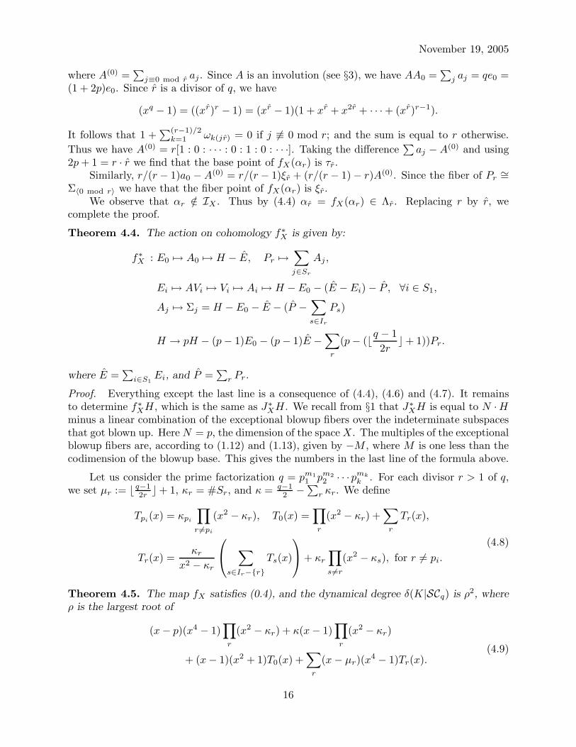
Theorem 4.4. The action on cohomology f∗X is given by:

f∗X : E0 7→ A0 7→ H − E, Pr 7→

∑

j∈Sr

Aj ,

Ei 7→ AVi 7→ Vi 7→ Ai 7→ H − E0 − (E − Ei) − P , ∀i ∈ S1,

Aj 7→ Σj = H − E0 − E − (P −∑

s∈Ir

Ps)

H → pH − (p − 1)E0 − (p − 1)E −∑

r

(p − (⌊q − 1

2r⌋ + 1))Pr.

where E =∑

i∈S1Ei, and P =

∑r Pr.

Proof. Everything except the last line is a consequence of (4.4), (4.6) and (4.7). It remainsto determine f∗

XH, which is the same as J∗XH. We recall from §1 that J∗

XH is equal to N ·Hminus a linear combination of the exceptional blowup fibers over the indeterminate subspacesthat got blown up. Here N = p, the dimension of the space X. The multiples of the exceptionalblowup fibers are, according to (1.12) and (1.13), given by −M , where M is one less than thecodimension of the blowup base. This gives the numbers in the last line of the formula above.

Let us consider the prime factorization q = pm1

1 pm2

2 · · · pmk

k . For each divisor r > 1 of q,we set µr := ⌊ q−1

2r ⌋ + 1, κr = #Sr, and κ = q−12 −

∑r κr. We define

Tpi(x) = κpi

∏

r 6=pi

(x2 − κr), T0(x) =∏

r

(x2 − κr) +∑

r

Tr(x),

Tr(x) =κr

x2 − κr

∑

s∈Ir−r

Ts(x)

+ κr

∏

s6=r

(x2 − κs), for r 6= pi.

(4.8)

Theorem 4.5. The map fX satisfies (0.4), and the dynamical degree δ(K|SCq) is ρ2, whereρ is the largest root of

(x − p)(x4 − 1)∏

r

(x2 − κr) + κ(x − 1)∏

r

(x2 − κr)

+ (x − 1)(x2 + 1)T0(x) +∑

r

(x − µr)(x4 − 1)Tr(x).

(4.9)

16

November 19, 2005

Proof. We have found hooks for all the exceptional hypersurfaces of fX , so (0.4) holds byTheorem 1.4. The proof that formula (4.9) gives characteristic polynomial of f∗

X is given inAppendix E.

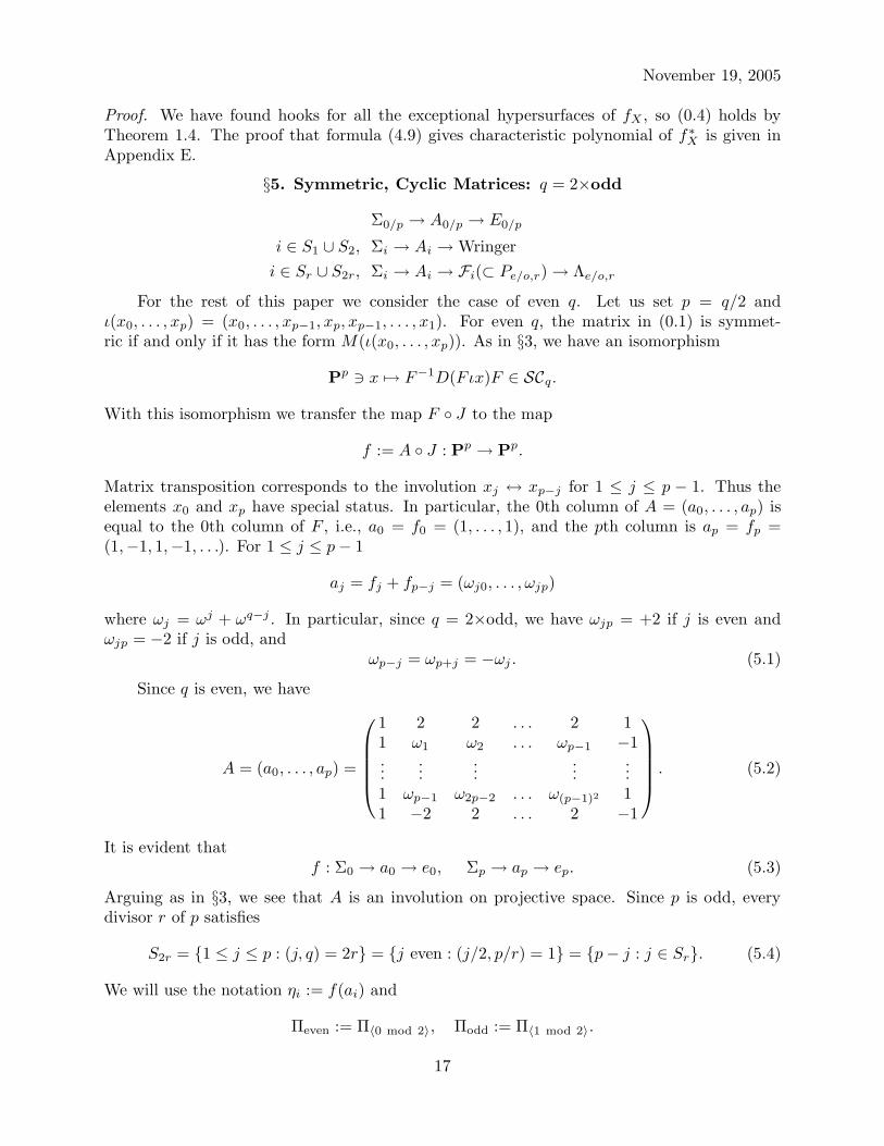
§5. Symmetric, Cyclic Matrices: q = 2×odd

Σ0/p → A0/p → E0/p

i ∈ S1 ∪ S2, Σi → Ai → Wringer

i ∈ Sr ∪ S2r, Σi → Ai → Fi(⊂ Pe/o,r) → Λe/o,r

For the rest of this paper we consider the case of even q. Let us set p = q/2 andι(x0, . . . , xp) = (x0, . . . , xp−1, xp, xp−1, . . . , x1). For even q, the matrix in (0.1) is symmet-ric if and only if it has the form M(ι(x0, . . . , xp)). As in §3, we have an isomorphism

Pp ∋ x 7→ F−1D(Fιx)F ∈ SCq.

With this isomorphism we transfer the map F J to the map

f := A J : Pp → Pp.

Matrix transposition corresponds to the involution xj ↔ xp−j for 1 ≤ j ≤ p − 1. Thus theelements x0 and xp have special status. In particular, the 0th column of A = (a0, . . . , ap) isequal to the 0th column of F , i.e., a0 = f0 = (1, . . . , 1), and the pth column is ap = fp =(1,−1, 1,−1, . . .). For 1 ≤ j ≤ p − 1

aj = fj + fp−j = (ωj0, . . . , ωjp)

where ωj = ωj + ωq−j . In particular, since q = 2×odd, we have ωjp = +2 if j is even andωjp = −2 if j is odd, and

ωp−j = ωp+j = −ωj . (5.1)

Since q is even, we have

A = (a0, . . . , ap) =

1 2 2 . . . 2 11 ω1 ω2 . . . ωp−1 −1...

......

......

1 ωp−1 ω2p−2 . . . ω(p−1)2 11 −2 2 . . . 2 −1

. (5.2)

It is evident thatf : Σ0 → a0 → e0, Σp → ap → ep. (5.3)

Arguing as in §3, we see that A is an involution on projective space. Since p is odd, everydivisor r of p satisfies

S2r = 1 ≤ j ≤ p : (j, q) = 2r = j even : (j/2, p/r) = 1 = p − j : j ∈ Sr. (5.4)

We will use the notation ηi := f(ai) and

Πeven := Π〈0 mod 2〉, Πodd := Π〈1 mod 2〉.

17

November 19, 2005

Lemma 5.1. If i ∈ S1, then ηi ∈ Πodd. If i ∈ S2, then ηi ∈ Πeven.

Proof. Let us consider first the case i = 2 ∈ S2. We will show that v2 = [1 : 0 : ±1 : 0 : ±1 : 0 :· · ·], which evidently belongs to Πeven. Note that ω := ω2 is a primitive pth root of unity, andsince p is odd, −ω is a primitive pth root of −1. We will solve the equation Ja2 = Av2 withv2 = [1 : 0 : t2 : 0 : t4 : 0 : · · ·]. Since q = 2p, we have Ja2 = [1 : 2/ω2 : 2/ω4 : · · · : 2/ω2p−2 : 1].

Thus the equation Ja2 = Av2 becomes the system of equations ω2i(1+∑(p−1)/2

j=1 ω2ijt2j) = 2t2for 0 ≤ i ≤ p. Now we repeat the proof of Lemma 4.1 with q replaced by p and with ω replacedby ω, and we find solutions t2j = ±1. This yields v2 ∈ Πeven, as desired. Finally, we pass fromthe case i = 2 to the case of general i ∈ S2 by repeating the arguments of Lemma 3.2.

Now consider i = 1 ∈ S1. We have Ja1 = [1 : 2/ω1 : 2/ω2 : · · · : 2/ωp−1 : −1]. Sincep − 1 ∈ S2, we have ηp−1 = [1 : 0 : t2 : 0 : · · · : tp−1 : 0] ∈ Πeven. The equation satisfied byvp−1 is ωk(p−1)(1 +

∑t2jω2jk) = tp−1 for 0 ≤ k ≤ p. Using (5.1), we convert this equation to

ωk(∑

t2jωp−2jk − 1) = tp−1, if k is odd

ωk(∑

t2jω2jk + 1) = tp−1, if k is even.

By (3.2) and (5.1) we have ωp−2j(2ℓ+1) = ωp−2j(2ℓ+1)+2ℓp and ω2j·2ℓ = ω2ℓp−2ℓ2j . Now settingk = 2ℓ + 1 when k is odd and k = 2ℓ when k is even, we have

ω2ℓ+1(∑

t2jω(2ℓ+1)(p−2j) − 1) = 2tp−1

ω2ℓ(∑

t2jω(2ℓ)(p−2j) + 1) = 2tp−1

It follows that η1 = [0 : tp−1 : 0 : tp−3 : · · · : t2 : 0 : 1] ∈ Πodd. For general i ∈ S1, we use theargument of Lemma 3.2.

Lemma 5.2. Let r be an odd divisor of q. For j ∈ Sr, we have ηj := faj ∈ Π〈r mod 2r〉, andη2j := fa2j ∈ Π〈0 mod 2r〉.

Proof. First we consider i = 2r ∈ S2r. Since ω = ω2r is a primitive (p/r)th root of unity, andp/r is odd, we repeat the proof of Lemma 4.1 to show that fa2r = η2r where η2r = [1 : 0 : · · · :0 : ±1 : 0 : · · ·] ∈ Π〈0 mod 2r〉. The same reasoning as in Lemma 3.2 shows that for generali ∈ S2r we have fai = ηi ∈ Π〈0 mod 2r〉

Now consider i = r ∈ Sr. Since p/r is odd ω = ωr is a primitive p/rth root of −1. Asbefore Jar = [1 : 2/ωr : 2/ω2r : · · · : 2/ω(p−1)r : −1]. With the same argument in the proof ofLemma 5.1 we have

ωk(∑

t2j ωk(p/r−2j) − 1) = 2tp/r−1, if k is odd

ωk(∑

t2j ωk(p/r−2j) + 1) = 2tp/r−1, if k is even.

By the definition of ωk we have

ωkr(∑

t2jωkr(p/r−2j) − 1) = 2tp/r−1, if k is odd

ωkr(∑

t2jωkr(p/r−2j) + 1) = 2tp/r−1, if k is even

which means far = ηr ∈ Π〈r mod 2r〉. For general i ∈ Sr, we use the argument of Lemma 3.2.

18

November 19, 2005

Lemma 5.3. We have:

AΠodd = x0 = −xp, x1 = −xp−1, . . . , x(p−1)/2 = −x(p+1)/2

AΠeven = x0 = xp, x1 = xp−1, . . . , x(p−1)/2 = x(p+1)/2,

and fAΠodd = Πodd, fAΠeven = Πeven.

Proof. Let us first consider the case AΠodd. A linear subspace AΠodd is spanned by columnvectors a1, a3, . . . , ap. When j is odd, aj = [2 : ωj : ω2j : · · · : ω(p−1)j : −2]. By (5.1)we have ω(p−k)j = ωpj−kj = −ωkj for all 1 ≤ k ≤ p − 1. It follows that AΠodd ⊂ x0 =−xp, x1 = −xp−1, . . . , x(p−1)/2 = −x(p+1)/2. Since A is invertible a1, a3, . . . , ap is linearlyindependent. It follows that

dim AΠodd =p + 1

2= dim x0 = −xp, x1 = −xp−1, . . . , x(p−1)/2 = −x(p+1)/2.

With the fact that ω(p−k)j = ωkj for even j, the proof for AΠeven is similar.With this formula for AΠodd, we see that it is invariant under J . Now since A is an

involution, we have fAΠodd = Πodd.

Let us construct the complex manifold π : X → Pp by a series of blow-ups. First we blowup the points e0, ep and aj for all j. Next we blow up the subspaces Πeven, Πodd, AΠeven,and AΠodd. Then we blow up the subspaces Π〈0 mod 2r〉, Π〈r mod 2r〉 and Π〈0 mod r〉 for allr /∈ S1 ∪ S2. We continue with our convention that if r2 divides r1 then we first blow upΠ〈0 mod 2r1〉, Π〈r1 mod 2r1〉, then Π〈0 mod r1〉, and then the corresponding spaces for r2. Wewill use the following notation for (π-exceptional) divisors of the blowup:

π : Pe → Πe, APe → AΠe, Po → Πo, APo → AΠo,

and for every proper divisor r of p we will write:

π : Pe,r → Π〈0 mod 2r〉, Po,r → Π〈r mod 2r〉, Pr → Π〈0 mod r〉.

For 1 ≤ i ≤ p − 1, we let Fi = F(ηi) denote the fiber over ηi. We define Λr as the stricttransform of AΣ〈0 mod r〉 in X, and Λe/o,r as the strict transforms of AΣ〈0/r mod 2r〉.

We will do two things in the rest of this Section: we will compute f∗X on Pic(X), and

we will show that fX : X → X is 1-regular. It is frequently a straightforward calculation todetermine f∗

X and more difficult to show that the map is 1-regular. Let us start by computingf∗

X . We will take H = HX , E0/p, Ai, i = 0, . . . , p, Pe/o, APe/o, Pe/o,r, Pr as a basis for Pic(X).We see that Σ0 contains ep as well as Πodd, as well as Π〈r mod 2r〉 ⊂ Πodd; and Σ0 contains noother centers of blow-up. Thus we have

H = Σ0 + Ep + Po, where Po = Po +∑

r

Po,r. (5.5)

This gives

f∗X : E0 7→ A0 7→ Σ0 = H − Ep − Po, Ep 7→ Ap 7→ Σp = H − E0 − Pe, (5.6)

19

November 19, 2005

where Pe = Pe +∑

r Pe,r. Next, consider a divisor r of p = q/2, so r is odd. If i ∈ Sr, then iis odd, and the set Σi contains the following centers of blowup: e0, ep, Πeven, Π〈s mod 2s〉 andΠ〈0 mod s〉 for all s which divide p but not r. Thus we have

H = Σi + E0 + Ep + Pe − (Po −∑

j∈Ir

Po,j) − (P −∑

j∈Ir

Pj) (5.7)

where Ir is the set of numbers 1 ≤ k ≤ p − 1 which divide r, and P =∑

r Pr. Thus we have

i ∈ Sr f∗X : Ai 7→ H − E0 − Ep − Pe − (Po −

∑

j∈Ir

Po,j) − (P −∑

j∈Ir

Pj)

i ∈ S2r Ai 7→ H − E0 − Ep − Po − (Pe −∑

j∈Ir

Pe,j) − (P −∑

j∈Ir

Pj)(5.8)

By a similar argument, we have

i ∈ S1 f∗X : Ai 7→ H − E0 − Ep − Pe − (Po − Po) − P

i ∈ S2 Ai 7→ H − E0 − Ep − Po − (Pe − Pe) − P(5.9)

If i ∈ S1, then fai ∈ Πodd. Further fAΠodd = Πodd and fXΠo = AΠe. We observe thatfor every divisor r, we have Pr → Λr, Pe/o,r → Λe/o,r, so APo and Ai, i ∈ S1 are the onlyexceptional hypersurfaces which is mapped by fX to π−1(Πodd). Thus we have

f∗X : Po 7→ APo +

∑

i∈S1

Ai, Pe 7→ APe +∑

i∈S2

Ai, APe/o 7→ Po/e (5.10)

For a divisor r of p we have

f∗X : Pe,r 7→

∑

i∈S2r

Ai, Po,r 7→∑

i∈Sr

Ai, and Pr 7→ 0 (5.11)

By §1, we have

f∗X : H 7→ pH − (p − 1)(E0 + Ed) − (p − (p + 1)/2)(Pe + Po)

−∑

r

(p − (p/r + 1)/2)(Pr,e + Pr,o) −∑

r

(p − p/r − 1)Pr(5.12)

Theorem 5.4. Equations (5.5–12) define f∗X as a linear map of Pic(X).

Next we discuss the exceptional locus of the induced map fX : X → X. As in §3, we have

fX : Σ0 → A0 → E0 → AΣ0, and Σp → Ap → Ep → AΣp.

Using (1.5), (1,6) and (1.8), we see that Σ0/p, A0/p, and E0/p are not exceptional.

20

November 19, 2005

Lemma 5.5. For i ∈ S1 ∪ S2, Σi is not exceptional for fX , and fX |Ai : Ai → Fi ⊂ Pe/o is adominant map; thus Ai is exceptional.

Lemma 5.6. fX : Pe → APo → Po → APe → Pe is a dominant map. In particular, Pe, APo,Po, and APe are not exceptional.

Proof. Since AΠodd and AΠeven are not indeterminate, it is sufficient to show that only for Pe

and Po. We will show the mapping fX : Pe → APo is dominant. The proof for Po is similar.The generic point of Pe is written as x; ξ where x = [x0 : 0 : x2 : 0 : · · · : xp−1 : 0] andξ = [0 : ξ1 : 0 : ξ3 : · · · : 0 : ξp]. It follows that fX(x; ξ) =

∑i: odd(1/ξi)ai;

∑j: even(1/xj)aj . It

is evident that the mapping is dominant and thus Pe is not exceptional.

Σ

Σ

ε

ε

F

F

Figure 5.1. Exceptional Orbits: The Wringer.

By Lemma 5.6, there is a 4-cycle Pe, APo, Po, APe of hypersurfaces, which we call “thewringer”; this is pictured in Figure 5.1. For i ∈ S1, the orbit fX : Σi → Ai → Fi entersthis 4-cycle, which illustrates Lemma 5.5. The fibers ε ⊂ Pe are the fibers F(ej) for even j,1 < j ≤ p − 1, and the fibers ε = F(ei) ⊂ Po correspond to i odd. If, for some n ≥ 0, we havefn

XFi ⊂ ε ⊂ IX , then the next iteration will blow up to a hypersurface.Let us identify Πe, and Πo, with Pp, p = (p − 1)/2 as follows:

i1 : [x0 : 0 : x2 : 0 : · · · : xp−1 : 0] ∈ Πe ↔ [x0 : x2 : · · · : xp−1] ∈ Pp

i2 : [0 : x1 : 0 : x3 : · · · : 0 : xp] ∈ Πo ↔ [xp : xp−2 : · · · : x1] ∈ Pp(5.13)

Thus we may identify ιe := (i1, i2) : Pe∼= Πe; Πo → Pp ×Pp and ιo := (i2, i1) : Po

∼= Πo; Πe →Pp × Pp. The number q = q/2 is odd, so the map fq = Aq J on Pp is one of the mapsdiscussed in §4. Let us define:

h1 := Pp ×Pp ∋ (x ; ξ) 7→ (fq(ξ) ; fq(x)) ∈ Pp × Pp

h2 := Pp ×Pp ∋ (x ; ξ) 7→ (fq(x) ; Aq φx(ξ)) ∈ Pp × Pp(5.14)

where for each v = [v0 : · · · : vp] ∈ Pp we set φv : [w0 : · · · : wp] 7→ [w0v−20 : · · · : wpv

−2p ]. If we

set h := h2 h1, then since i2 reverses the coordinates, we have

f2X = ι−1

o h ιe on Pe, and f2X = ι−1

e h ιo on Po.

21

November 19, 2005

In other words, ιe and ιo conjugate the action of f2X on the wringer to the map h on Pp ×Pp.

If i ∈ S2, then ı = i/2 is relatively prime to q, and we write vı ∈ Pp for the vector inLemma 3.2. Thus we have ιe(ηi) = vı, and we have ιeFi = vı × Pp. Similarly, if i ∈ S1,ı = (p − i)/2 is relatively prime to q, and we have ιo(ηi) = vı, and we may identify Fi withthe vertical fiber over vı.

For x ∈ Pp, let L(x) ⊂ Pp denote the line containing a0 = (1, . . . , 1) and x. Recall thatvı = [1 : ±1 : ±1 : · · ·] = [1 : t1 : · · · : tp], and define the set Iı = 1 ≤ k ≤ p : tk = −1. Itfollows that L(eı) = x0 = xk, k 6= ı, and

L(vı) = [x0 : · · · : xp] : x0 = xk, k /∈ Ii; xℓ = xm, ℓ, m ∈ Iı.

Thus L(eı) = [x0 : x0 : · · · : x1 : · · · : x0], where all the entries are x0, except for one x1 inthe ı location, and L(vı) = [x0 : · · · : x1 : · · ·], where all the entries are x0 except for a x1 ineach location in Iı.

If i ∈ S1 ∪ S2, we write Bi := L(vı) × L(vı) and Di = L(eı) × L(eı).

Lemma 5.7. h : Bi ↔ Di.

Proof. Let us first consider h(Bi). Using defining equations for L(vı) we have that 1 dimen-sional linear subspace L(vı) is invariant under J . Thus fqL(vı) is a linear subspace containingfqa0 = e0 and fq vı. Let us sset fq vı = [α0 : · · · : αp]. It follows that fqL(vı) = [x0 : · · · :xp] : αkx1 = α1xk, k = 2, . . . , p and JfqL(vı) = [x0 : · · · : xp] : α1x1 = αkxk, k = 2, . . . , p.Since JfqL(vı) is again a 1 dimensional linear subspace, we have f2

q L(vı) = Aq JfqL(vı) isa linear subspace. Note that e0 ∈ JfqL(vı) and Aqe0 = a0. By the Theorem 3.3, we havef2

q vı = eı. Thus we have f2q L(vı) = L(eı). Now consider a generic point in h1L(vı). By

the previous computation a generic point in h1L(vı) is [y0 : · · · : yp]; [ζ0 : · · · : ζp] whereαky1 = α1yk and αkζ1 = α1ζk for k = 2, . . . , p. It follows that α1(ζ1/y2

1) = αk(ζk/y2k). Thus

we have Aq φy(ζ) ∈ L(eı) and therefore h(Bi) = Di.For h(Di), we note that L(eı) is invariant under J and Aq, J are both involutions. Using

the previous argument, we have AqJAqL(vı) = L(eı) = JL(eı) and therefore f2q L(eı) = L(vı).

Recall that fqL(eı) = [x0 : · · · : xp] : α1x1 = αkxk, k = 2, . . . , p, and with the same reasoningfor fqL(vı), we have h(Di) = Bi.

By Lemma 5.7, we may simplify notation and write h|Bi and h|Di in the form

h([x0 : x1], [y0 : y1]) = ([x′0 : x′

1], [y′0 : y′

1]).

For the following we write h in affine coordinates h(x, y) = (x′, y′). In order to write h|Bi andh|Di more explicitly, we will use the following result:

Lemma 5.8. For i ∈ S1 ∪ S2, we set α(i) :=∏p

ℓ=1

∑j∈Iı

ωjℓ and β(i) :=∏p

ℓ=1 ωℓı. It follows

that (α(i))2 = (β(i))2 = 1, and the coefficient tı = ±1 in vı satisfies

p∑

k=1

∏

ℓ 6=k

∑

j∈Iı

ωjℓ = tıα(i),

p∑

k=1

ωk

∏

ℓ 6=k

∑

j∈Iı

ωjℓ = (2 − p)tıα(i)

p∑

k=1

∏

ℓ 6=k

ωjℓı = ⌊p + 1

2⌋tıβ

(i),

p∑

k=1

ω2kı

∏

ℓ 6=k

ωℓı = −(1 + 2⌊p + 1

2⌋)tıβ

(i).

22

November 19, 2005

Proof. Recall that for each i ∈ S1 ∪ S2, we have ı ∈ S1(q) and vı = [1 : t1 : · · · : tp] = [1 : ±1 :· · · : ±1] and Aq vı = [α0 : · · · : αp] where α0 = 1+2

∑tj and αk = 1+

∑tjωjk. Since tk = ±1

and 1 +∑

ωjk = 0 for all k 6= 0, it follows that 1 +∑

tjωjk = −2∑

j∈Iıωjk. By Lemma 3.2,

we have Jaı = Aq vı and α0 = tı. It follows that [tı : 2tı/ωı : · · · : 2tı/ωpı] = [tı : −2∑

j∈Iıωj :

· · · : −2∑

j∈Iıωpj ] and therefore we have

∑

j∈Iı

ωkj = −tı/ωkı. (5.15)

Thus we have α(i) = (−tı)p∏p

ℓ=1 1/ωℓı. Recall that ωj = ωj +ωq−j is real for all j and tı = ±1.

Since ωı is a qth primitive root of unity, we have xq − 1 = (x − 1)∏q−1

ℓ=1(x − ωℓı). By lettingx = −1 we get

|α(i)|2 =1

|β(i)|2=

p∏

ℓ=1

1

ωℓı · ωq−ℓı

p∏

ℓ=1

1

(1 + ωq−ℓı)(1 + ωℓı)= 1

Notice that∑p

k=1

∏ℓ 6=k

∑j∈Iı

ωjℓ = (−tı)α(i)∑p

k=1 ωkı = tıα(i). Similarly we have

∑pk=1 ωk

∏ℓ 6=k

∑j∈Iı

ωjℓ = (−tı)α(i)∑p

k=1 ω2kı. Recall that ω2

kı = 2 + ω2kı and 2ı is rela-

tively prime to q. It follows that∑p

k=1 ω2kı = 2p − 1 = p − 2.

Note that∑p

k=1

∏ℓ 6=k ωℓı =

∏ℓ ωℓı

∑pk=1 1/ωkı. By (5.15) we have

∑pk=1

∏ℓ 6=k ωℓı =

(−tı)∏

ℓ ωℓı

∑j∈Iı

∑pk=1 1/ωkj. Recall (3.4), we have #Iı = ⌊(p + 1)/2⌋. It follows that

∑pk=1

∏ℓ 6=k ωℓı = tı⌊(p + 1)/2⌋

∏pℓ=1 ωℓı. Using (3.2) we have ω2kı + 2 = ω2

kı. It follows that∑p

k=1 ω2kı

∏ℓ 6=k ωℓı =

∏ℓ ωℓı

∑pk=1 ωkı − 2

∑pk=1

∏ℓ 6=k ωjℓı. By the previous computation, it

follows that∑p

k=1 ω2kı

∏ℓ 6=k ωℓı = −(1 + 2⌊ p+1

2 ⌋)tı∏p

ℓ=1 ωℓı.

Lemma 5.9. If p is even, then

h|Bi =

(−p + (−p + 1)y

1 + y,y2 − 2xy + p2(x − 1)(y + 1)2 + x + p(x − 1)(y2 − 1)

2y2 − p(x − 1)(y + 1)2 − x(y2 + 2y − 1)

)

h|Di =

(−py − 1

(p − 1)y + 1,

2p2(y − 1)x2 + x2 − p(x − 4)(y − 1)x − 2yx + 3y − 2

(2(1 − y)p2 − 3(1 − y)p + 2 − y)x2 + (−4yp + 4p + 2y − 4)x − y + 2

)

and a similar formula holds for p odd.

Proof. This is a direct calculation using the definitions of h1 and h2 and the identities onLemma 5.8.

Lemma 5.10. If i ∈ S1 ∪ S2, then the point (−1, 1) ∈ Bi is preperiodic, that is h(−1, 1) hasperiod 4. Thus (−1, 1) ∈ Bi is a hook for Ai.

Proof. The preperiodicity of (−1, 1) follows from the formula in Lemma 5.9. To see that(−1, 1) is a hook, we argue as follows: Suppose i is even. Then fXAi = Fi ⊂ Pe, and Fi is thefiber over ηi. We need to show that for all n ≥ 0, fn

XFi 6⊂ IX . We have identified ιe : Pe →Pp ×Pp, and under this identification F(ηi) is taken to vı ×Pp. Thus ιe(Fi)∩Bi correspondsto the line [1 : −1] ×Pp, which contains the point which we represent in affine coordinates as

23

November 19, 2005

(−1, 1). Although it is true that h1(−1, 1) corresponds to a point of indeterminacy of fX , therest of h1([1 : −1] × P1) is disjoint from IX . It follows that h([1 : −1] × P1) is a curve in Di

which passes through h(−1, 1). Since the 4-cycle h(−1, 1), h2(−1, 1), h3(−1, 1), h4(−1, 1) isdisjoint from IX , our result follows.

From §1 we have the following:

Lemma 5.11. When r is a proper divisor of p, fX induces dominant maps Pe,r → Λe,r,Po,r → Λo,r, and Pr → Λr. In particular, the hypersurfaces Pe,r, Po,r, and Pr are exceptional.

Next we will construct hooks for the subspaces Pe,r, Po,r, and Pr. Let us define τ ′ = [t′0 :· · · : t′p] and τ ′′ = [t′′0 : · · · : t′′p ] where t′0 = −t′p = t′′0 = t′′p = −(pr − p)/(p + r), t′jp/r = (−1)j ,

t′′jp/r = 1 for 1 ≤ j ≤ r − 1, and t′i = t′′i = 0 for all other i. We set

τe,r := τ ′ + τ ′′ ∈ Π〈0 mod 2 p

r〉, τo,r := τ ′ − τ ′′ ∈ Π〈 p

rmod 2 p

r〉.

Lemma 5.12. We have τ ′ =∑

i odd, i 6≡0 mod r ai and τ ′′ =∑

i even, i 6≡0 mod r ai. Thus

τe,r, τo,r ∈ AΣ〈0 mod 2r〉 ∩ AΣ〈r mod 2r〉 = AΣ〈0 mod r〉.

Proof. Since ω is a pth root of −1, we have

(ωp + 1) = −(ω + 1)(−1 + ω − ω2 + · · ·+ ωp−2 − ωp−1) = 0.

We also have ωq−k = ωp · ωp−k = −ωp−k, so ω1 − ωp−1 = ω1 + ωq−1 = ω1, ω3 − ωp−3 =ω3 + ωq−3 = ω3, . . . and −ω2 + ωp−2 = ωp+2 + ωp−2 = ωp−2, etc. It follows that

−1 + ω − ω2 + · · · + ωp−2 − ωp−1 = ω1 + ω3 + · · · + ωp−2 − 1 = 0.

Similarly for all odd k 6= p, ωk is a pth root of −1 and∑

i odd ωki − 1 = 0.Since ω2 is a pth root of unity, we have

((ω2)p − 1) = (ω2 − 1)(1 + ω2 + ω4 + · · ·+ ω(p−1)2) = 0.

Since ωq−2k = ω2p−2k, we have ω2 + ω(p−1)2 = ω2. Similarly, ω4 + ω(p−2)2 = ωq−2(p−2) +ω(p−2)2 = ω(p−2)2, etc. It follows that

1 + ω2 + ω4 + · · · + ω(p−1)2 = ω2 + ω6 + · · · + ω(p−1)2 + 1 = 0.

For all even k 6= 0 we have∑

i odd ωki + 1 = 0, and we may combine the cases of k even andodd to obtain ∑

i odd

ai = (p + 1)[1 : 0 : · · · : 0 : −1].

Since r is a divisor of p, ωr is a primitive p/rth root of −1 and ((ωr)p/r + 1) = (ωr + 1)(1 −ωr + ω2r + · · ·+ ω(p/r−1)r). Repeating the previous argument with ωr and p/r, we have

∑

i odd, i≡0 mod r

ai = (p/r + 1)[1 : 0 : · · · : 0 : −1 : 0 : · · · : 0 : 1 : 0 : · · · : −1] ∈ Π〈0 mod p/r〉.

Subtracting∑

i odd ai from∑

i odd, i≡0 mod r ai, it follows that τ ′ =∑

i odd, i 6≡0 mod r ai ∈AΣ〈0 mod r〉. The proof for τ ′′ is similar.

Let us define u′e,r = (u′

i) ∈ Pp to be the vector such that u′i = 1 if i ≡ p/r mod 2p/r and

u′i = 0 otherwise. We set u′′

e,r = (u′′i ) where u′′

i = 0 if i ≡ 0 mod p/r and u′′i = 1 otherwise.

Let us define u′o,r = (u′

i) ∈ Pp to be the vector such that u′i = 1 if i ≡ 0 mod 2p/r and u′

i = 0

otherwise. We set u′′o,r = (u′′

i ) where u′′i = 0 if i ≡ 0 mod p/r and u′′

i = (−1)i otherwise. Welet ℓe,r to be the line containing u′

e,r and u′′e,r, and let αe,r be the line in Pe,r lying over the

basepoint τe,r and having fiber coordinate in ℓe,r. We define αo,r similarly.

24

November 19, 2005

Lemma 5.13. Each of the sets αe,r∩IX and αo,r∩IX consists of 2 points, and αe,r∪αo,r ⊂ Λr.fXαe,r ⊂ Pr ∩ Λe,r, and fXαo,r ⊂ Pr ∩ Λo,r. Finally, f2

Xαe,r = αe,r, and f2Xαo,r = αo,r.

Proof. Let us consider the case αe,r. By Lemma 5.11, fX : Pe,r → Λe,r and by Lemma 5.12αe,r ⊂ Pe,r. It follows that fXαe,r ⊂ Λe,r. A generic point ζ in αe,r has a form τr,o + τr,e; [0 :1 : · · · : 1 : x : 1 : · · · : 1 : 0 : 1 : · · · 1 : x] for some x ∈ C∗. Applying the map f , we have

ζJ7→ [0 : 1 : · · · : 1 :

1

x: 1 : · · · : 1 : 0 : 1 : · · · : 1 :

1

x]; [

(p + r)

(pr − p): 0 : · · · : 0 : 1 : 0 : · · ·]

A7→ (τp/r,o + τp/r,e +

1

x

∑

i≡p/r mod 2p/r

ai); ((p + r)

(pr − p)a0 +

∑

i≡0 mod 2p/r

ai).

By Lemma 5.12, there exist nonzero constants β1, β2, and β3 such that

τp/r,o + τp/r,e +1

x

∑

i≡p/r mod 2p/r

ai ∈ Π〈0 mod r〉

=[β1 : 0 : · · · : 0 : β2 : 0 : · · · : 0 : β2 : 0 : · · · : 0] ∈ Π〈0 mod 2r〉

+ [β3

x: 0 : · · · : 0 : −

β3

x: 0 : · · · : 0 :

β3

x: 0 : · · ·] ∈ Π〈0 mod r〉.

It follows that fXαe,r ⊂ Pr ∩ Λe,r. Again by Lemma 5.11, we know that f2Xαe,r ⊂ Λr. For

the fiber for fXζ, the jth-coordinate of 1αa0 +

∑i≡0 mod 2p/r ai are all equal for j 6≡ 0 mod r.

It follows that

fX : ζ 7→ fXζ 7→ τr,o + τr,e; (1

β1 + β3/xa0 +

1

β2

∑

i≡r mod 2r

ai +1

β2 − β3/x

∑

i≡0 mod 2r

ai).

Note that both αe,r f2Xαe,r are 1-dimensional linear subspaces in fiber over τe,r. Using the

computation in Lemma 5.12 we have f2Xαe,r = αe,r. We use a similar argument for αo,r.

Corollary 5.14. Let r > 1 be an odd divisor of q. Then for j ∈ Sr, αo,r is a hook for Aj,and Po,r and Pr; and αe,r is a hook for A2j , Pe,r, and Pr.

Let us consider the prime factorization q = 2pm1

1 pm2

2 · · · pmk

k . For each divisor r > 1 of q,

we set µ := p+12 , κ = #S2 = #S1, µr := p/r+1

2 , and κr = #S2r = #Sr.

Theorem 5.15. Condition (0.4) holds for fX , and δ(K) = ρ2 where ρ is the largest root of

(x − p)(x2 − κ − 1)∏

r

(x2 − κr) + 2κ(x − µ)∏

r

(x2 − κr)

+ 2(x − 1)T0(x) + 2∑

r

(x − µr)(x2 − 1)Tr(x)

with the polynomials Tj(x) are defined in (4.8).

Proof. We have determined all the exceptional hypersurfaces for fX and have found a hook foreach of them. Thus by Theorem 1.4, condition (0.4) holds for fX . Thus δ(f) is the spectralradius of f∗

X . Consider f∗X as in Theorem 5.4 and let χ(x) denote its characteristic polynomial.

25

November 19, 2005

We may now determine χ(x) as in Theorem 4.5 (see Appendix E). We find that χ(x) is thepolynomial above times a polynomial whose roots all have modulus one.

§6. Symmetric, Cyclic Matrices: q = 2×even

Σ0/p → A0/p → E0/p

Σ p2

→ A p2

→ AΠodd → L

i ∈ S1 Σi → ai → ∗ ∈ A p2

i ∈ Sr ∪ S2r Σi → Ai → Fi ⊂ Pe/o,r → Λe/o,r

i ∈ Sρ Σi → Fi ⊂ Γρ → λi ⊂ Γρ

In this case we set p = q/2, and our mapping is given by f = A J , with A as in (5.2).Since q is divisible by 4, we have additional symmetries:

ωjp/2 = 0 if j is odd, ωjp/2 = (−1)j/2 if j is even, and ωp/2+j = −ωp/2−j (6.1)

As before, we haveΣ0 → a0 → e0, Σp → ap → ep. (6.2)

However, now we encounter the phenomenon that A contains several 0 entries, for instance

Σp/2 → ap/2 = [1 : 0 : −1 : 0 : 1 : 0 : · · ·] ∈ Πeven. (6.3)

We will write q = 2mqodd and consider two sorts of divisors ρ and r, which satisfy:

ρ|(q/4), and r = 2m−1r′, r′|qodd. (6.4)

We will use the notation ρ := q/(4ρ). Note that this is again a divisor of the form ρ.

Lemma 6.1. Suppose that r = 2m−1r′, and r′ divides qodd. If i ∈ Sr, then fai ∈ Π〈r mod 2r〉,and if j ∈ S2r, then faj ∈ Π〈0 mod 2r〉.

Proof. Since ω = ω2r is a primitive p/rth root of unity and p/r is odd, the proof is the sameas Lemma 5.2.

Lemma 6.2. Suppose that 1 < ρ < q/4 divides q/4. Then every i ∈ Sρ is an odd multiple ofρ, and we have Sρ = p − j : j ∈ Sρ, and ai ∈ Σ∗

〈ρ mod 2ρ〉.

Proof. Since 2ρ is also a divisor of q, every i ∈ Sρ is an odd multiple of ρ. Suppose j ∈Sρ, then we have j = kρ where gcd(k, q/ρ) = 1 and p − j = ρ(p/ρ − k). It follows thatgcd(p/ρ − k, q/ρ) = 1 and p − j ∈ Sρ. We observe that jρ · i = jρ · kρ = jk · q/4. By (6.1) itfollows that ωjρi = 0 if j is odd, ωjρi = ±2 if j is even, and ωji 6= 0 otherwise.

Lemma 6.3. If i ∈ S1, then ai ∈ Σ∗p/2.

Proof. Since i is relatively prime to q, i is odd and ωp/2·i = 0 by (6.1). ωi is a qth primitiveroot of unity, and therefore ω0, ω1, . . . , ωp = ω0i, ω1i, . . . , ωpi as a set. It follows that eachai has exactly one zero coordinate.

Now we construct the space π : X → Pp by a series of blowups. We blow up a0, e0, ap, ep,and ap/2. For each divisor of the form r in (6.4), we blow up ai for all i ∈ Sr ∪S2r. As before,

26

November 19, 2005

Ai denotes the blowup fiber of ai. We also blow up Π〈0 mod 2r〉 and Π〈r mod 2r〉; we denotethe blowup fibers as Pe,r and Po,r, respectively. For each divisor of the form ρ in (6.4) (orequivalently ρ), we blow up Σ〈ρ mod 2ρ〉; we denote the blowup fiber by Γρ. Let fX : X → Xdenote the induced birational map.

Let us take H = HX , E0/p, A0/p, A p2

, Ai, i ∈ Sr ∪ S2r, Pe/o,r, and Γρ as a basis forPic(X). As in §5, we have

f∗X : E0 7→ A0 7→ Σ0 = H − Ep − Po, Ep 7→ Ap 7→ Σp = H − E0 − Pe, (6.5)

where Pe/o =∑

r Pe/o,r. And for a divisor r of q in (6.4), we have

f∗X : Pe,r 7→

∑

i∈S2r

Ai, Po,r 7→∑

i∈Sr

Ai

i ∈ Sr Ai 7→ H − E0 − Ep − Pe − (Po −∑

j∈Ir

Po,j)

i ∈ S2r Ai 7→ H − E0 − Ep − Po − (Pe −∑

j∈Ir

Pe,j)

(6.6)

We see that Σp/2 contains e0/p, Π〈0 mod 2r〉 and Π〈r mod 2r〉 as well as Γρ. Let us suppose

q = 2m · odd. We set Γ =∑

ρ:2m−2·odd Γρ. Since aj ∈ Σp/2 for all odd j, if p/2 is odd we have

H = Σp/2 + E0 + Ep + Pe + Po + Γ + Ap/2. (6.7)

Thus we have

f∗X : Ap/2 7→ Σp/2 = H − E0 − Ep − Pe − Po − Γ − Ap/2 if p/2 is odd

Ap/2 7→ Σp/2 = H − E0 − Ep − Pe − Po − Γ if p/2 is even(6.8)

Let us consider a divisor ρ of q in (6.4). We have

f∗X : Γρ 7→

∑

i∈Sρ

Σi. (6.9)

We observe that Σ〈ρ mod 2ρ〉 ⊂ Σodd·ρ and ap/2 = [1 : 0 : −1 : 0 : · · · : ±1] ∈ Σj for all odd j.Thus for i ∈ Sρ we have

ρ even Σi = H − E0 − Ep − Pe − Po − Γρ,

ρ odd Σi = H − E0 − Ep − Ap/2 − Pe − Po − Γρ.(6.10)

Thus we have

ρ even f∗X : Γρ 7→

∑

i∈Sρ

Σi = #Sρ(H − E0 − Ep − Pe − Po − Γρ),

ρ odd Γρ 7→∑

i∈Sρ

Σi = #Sρ(H − E0 − Ep − Ap/2 − Pe − Po − Γρ).(6.11)

By §1, we have

f∗X : H 7→ pH − (p − 1)(E0 + Ed) − (p − (p/2 + 1))Ap/2

−∑

r

(p − (p/r + 1)/2)(Pe,r + Po,r) −∑

ρ

(ρ − 1)Γρ(6.12)

This accounts for all of the basis elements of Pic(X), so we have:

27

November 19, 2005

Theorem 6.4. Equations (6.5–12) define f∗X as a linear map of Pic(X).

Let us set L = ap/2; Πodd ⊂ Ap/2.

Lemma 6.5. fX : Ap/2 → AΠodd ⊂ Σp/2, AΠodd 6⊂ IX , and fX : AΠodd → L. In particular,f2

X defines a dominant map of L to itself.

Proof. A generic point of an exceptional divisor Ap/2 can be expressed as ap/2; ξ = [1 : 0 : −1 :0 : · · ·]; [ξ0 : ξ1 : ξ2 : · · ·]. Thus we have

fX(ap/2; ξ) = A[0 : 1/ξ1 : 0 : 1/ξ3 : 0 : · · · : 1/ξp−1 : 0] =∑

i: odd

1

ξiai ∈ AΠodd.

From the computation, it is clear that the rank of fX |Ap/2 is equal to the dimension of AΠodd.With (6.1) and the same reasoning as in Lemma 5.3, we have

AΠodd = x0 = −xp, x1 = −xp−1, . . . , xp/2−1 = −xp/2+1, xp/2 = 0

Now the generic point x of AΠodd is x = [x0 : x1 : · · · : xp/2−1 : 0 : −xp/2−1 : · · · : −x0], andAΠodd ⊂ Σp/2. Now

fX(x) = ap/2; A[1/x0 : · · · : 1/xp/2−1 : 0 : −1/xp/2−1 : · · · : −1/x0] ∈ L,

and the mapping is dominant. By the previous computation for Ap/2, f2X : L → L is dominant.

From §1 we have the following:

Lemma 6.6. Let r be a divisor of the form (6.4). If i ∈ Sr, we let Fi denote the fiber ofPo,r over fai. In this notation, we have dominant maps: fX : Σi → Ai → Fi. In fact,for every fiber F of Po,r, fX : F → AΣ〈r mod 2r〉 is a dominant map. Similarly, supposej ∈ S2r. With corresponding notation, we have dominant maps fX : Σi → Ai → Fi ⊂ Pe,r

and fX : F → AΣ〈0 mod 2r〉.

Proposition 6.7. AΠodd ⊂ AΣ〈0 mod 2r〉 ∩ AΣ〈r mod 2r〉 is a hook for the spaces: Ap/2, andPe,r, Po,r, Ai, i ∈ Sr ∪ S2r, for every divisor r in (6.4).

Lemma 6.8. fXa1 = ap/2; [0 : p − 1 : 0 : 3 − p : 0 : p − 5 : 0 : · · · : ±1 : 0] ∈ L. If i ∈ S1, thenfXai is obtained from fXa1 by permuting the nonzero coordinates.

Proof. Using Lemma 6.3 and 6.5 which show that fXa1 ∈ L, we can set fXa1 = ap/2; [0 : ξ1 :0 : ξ3 : 0 : · · · : ξp−1 : 0]. Recall that a1 = [2 : ω1 : · · · : ωp/2−1 : 0 : −ωp/2−1 : · · · : −2].

Applying fX we have ξk = 1 + 2∑p/2−1

j=1 ωkj ·1

ωjfor k = 1, 3, . . . , p − 1. If k = 1, we have

ξ1 = 1 + 2∑p/2−1

j=1 ωj/ωj = p − 1. For k ≥ 1, we will show that ξk + ξk+2 = (−1)(k−1)/22. Letus recall the last equality in (3.2). ωj · ω(k+1)j = ω(k+1)j−j + ω(k+1)j+j = ωkj + ω(k+2)j. Itfollows that

ξk + ξk+2 = 2 + 2

p/2−1∑

j=1

(ωkj + ω(k+2)j) ·1

ωj= 2 + 2

p/2−1∑

j=1

ω(k+1)j.

28

November 19, 2005

When k + 1 ≡ 2 mod 4, ω(k+1)j is a pth root of unity and therefore∑p/2−1

j=1 ω(k+1)j = 1 +∑p/2−1

j=1 ω(k+1)j − 1 = 0. If k + 1 ≡ 0 mod 4, ω(k+1)p/4+(k+1)j = (−1)(k+1)/4ω(k+1)j and∑p/2−1

j=1 ω(k+1)j + 2 = 0. Thus we get ξk + ξk+2 = 2 if k + 1 ≡ 2 mod 4, and ξk + ξk+2 = −2if k + 1 ≡ 0 mod 4. For general i ∈ S1, we use the same permutation argument as in Lemma

3.2. In fact, if we set fXai = ap/2; [0 : ξ(i)1 : 0 : ξ

(i)3 : · · ·], then ξ

(i)i = p− 1, and ξ

(i)k + ξ

(i)k+2i = 2

if k + i ≡ 2 mod 4, and ξ(i)k + ξ

(i)k+2i = −2 if k + i ≡ 0 mod 4.

Figure 6.1. An Exceptional Orbit: q = 12.In Figure 6.1 we consider q = 12, p = 6. Thus L has dimension 2, and we plot points of

the orbit f2n+1a1, n ≥ 0, in an affine coordinate chart inside L.Let us define i1 : Πodd ∋ [0 : x1 : 0 : · · · : xp−1 : 0] 7→ [x1 : x3 : · · · : xp−1] ∈ P

p

2−1 and

J1 := i−11 J

P

p2−1 i1 : Πodd → Πodd. Similarly, let i2 : AΠodd ∋ [x0 : x1 : · · · : xp/2−1 : 0 :

−xp/2−1 : · · · : −x0] 7→ [x0 : x1 : · · · : xp/2−1] ∈ Pp

2−1, and define J2 := i−1

2 JP

p2−1 i2 :

AΠodd → AΠodd. Now we define ϕ := i1(AJ2 AJ1)i−11 as a p/2-tuple of polynomials with

coefficients in Z[ω]. Thus ϕ is a map of Z[ω]p/2 to itself. The map ϕ also induces a map ofPp/2−1 to itself, and i1 conjugates this map of projective space to f2

X : L → L.

Lemma 6.9. For j ∈ S1, there is a polynomial Rj ∈ Z[ω] such that xj |Rj , and

ϕ[x1 : x3 : x5 : . . . : xp−1] = 2(p/2)2[p − 1 : 3 − p : · · · : ±1]x1p/2

+ R1(x)

= Vjxjp/2 + Rj(x)

where Vj is obtained from 2(p/2)2[p − 1 : 3 − p : · · · ;±1] by permuting the coordinates.

Proof. Let us set [y1 : y3 : · · · : yp−1] = ϕ[x1 : x3 : · · · : xp−1]. A direct computation gives that

yi is equal to 2(∑

s: odd xs)∏p/2−1

k=1 (∑

s: odd ωksxs) times

p/2−1∏

k=1

(∑

s: odd

ωksxs

)+ 2

(∑

s: odd

xs

)·

p/2−1∑

ℓ=1

ωjℓ

∏

k 6=ℓ

(∑

s: odd

ωksxs)

.

29

November 19, 2005

Recall that xs = 0 on⋃

j 6=sxj = 0 and xs 6= 0 on xs = 0 ∪⋂

j 6=sxj 6= 0. It follows thaton Σ∗

1,

yj = (

p/2−1∏

k=1

ωk)2 · [1 + 2

p/2−1∑

ℓ=1

ωjℓ ·1

ωℓ] · x1

p/2∀j : odd.

Let us write Ω =∏p/2−1

k=1 ωk. With the previous Lemma, it is clear that we have a polynomial

R1 such that x1 is a divisor of R1 and ϕ(x) = Ω[p−1 : 3−p : · · · : ±1]·x1p/2−1

+R1(x). We want

to show that Ω = ±p/2. Now Ω =∏p/2−1

k=1 ω−k(1 + ω2k) = (∏p/2−1

k=1 ω−k) · (∏p/2−1

k=1 1 + ω2k).Since ω is a primitive qth root of unity and 4 is a divisor of q we see that

q−1∏

k=1

ωk = ±(

p−1∏

k=1

ωk)2 = ±(

p/2−1∏

k=1

|ωk|)4 = 1.

For all 1 ≤ k ≤ p/2 − 1, ω2k is a p/2th root of −1 and therefore

(xp/2 + 1) = (x + 1)(1 − x + x2 − · · · + xp/2−1) = (x + 1)

p/2−1∏

k=1

(x − ω2k).

Setting x = −1, we have −p2 =

∏p/2−1k=1 (1 + ω2k). For j ∈ S1, we reason as in the proof of

Lemma 3.2.

Lemma 6.10. For i ∈ S1, fnXai /∈ IX for all n ≥ 0.

Proof. By Proposition 6.7, i1fXa1 = [p − 1 : 3 − p : p − 5 : · · · : ±1]. Let us set u1 =(p − 1, 3 − p, p − 5, · · · ,±1). It suffices to show that ϕn(u1) /∈ i1IX for all n ≥ 0. For this weneed to know that for each n, at most one coordinate of ϕnu1 can vanish. Let us choose aprime number p/2 < µ ≤ p − 1. One of the coordinates of u1 is equal to ±µ. Suppose it isthe jth coordinate. Then 2j − 1 must be relatively prime to q, so we can apply Lemma 6.9.Working modulo µ, we see that ϕu1 = bjuj , where uj is obtained from u1 by permuting the

coordinates, and bj = 2(p/2)2(u1)j

p/2. For each k 6= j, the kth coordinate of u1 is nonzero

modulo µ. Thus bj is a unit modulo µ, and so ϕu1 is a unit times a permutation of u1. Thepermutation preserves the set S1, so if j2 denotes the coordinate of i−1

1 ϕu1 which vanishesmodulo µ, then j2 ∈ S1. Thus we may repeat this argument to conclude that, modulo µ, ϕnu1

is equal to a unit times a permutation of u1. Thus at most one entry of ϕnu1 can vanish, evenmodulo µ.

From (5.1,2) and (6.1) we have the following:

Lemma 6.11. Consider a divisor ρ in (6.4). We have

AΠ〈ρ mod 2ρ〉 = x0 = −x2ρ = x4ρ = −x6ρ = · · · = ±x2ρρ,

x1 = −x2ρ−1 = −x2ρ+1 = x4ρ−1 = x4ρ+1 = · · · = ±x2ρρ−1, . . . ,

xρ−1 = −xρ+1 = −x3ρ−1 = x3ρ+1 = · · · = ±x2ρρ−ρ+1.

Proof. By (5.1,2) and (6.1), it is easy to check that aj , j ≡ ρ mod 2ρ satisfies all the equations.

30

November 19, 2005

Lemma 6.12. Consider a divisor of the form ρ in (6.4). Then AΠ〈ρ mod 2ρ〉 ⊂ Γρ. Let ususe the notation Λρ := π−1AΠ〈ρ mod 2ρ〉 for the exceptional fiber over AΠ〈ρ mod 2ρ〉. Then wehave a dominant mapping fX : Γρ → Λρ. Furthermore, f2

X : Λρ → Λρ is a dominant mapping,so Λρ is a hook for Γρ.

Proof. A linear subspace AΠ〈ρ mod 2ρ〉 is spanned by akρ, k :odd. For j odd, the jρ-th coordi-nate of akρ is ωjρ·kρ = ωjk·p/2 = 0 by (6.1). If follows that AΠ〈ρ mod 2ρ〉 ⊂ Γρ.

Let us conisder a generic point x; ξ in Γ∗ρ. Using the previous argument, it is clear that

the base of fX(x; ξ) is in AΠ〈ρ mod 2ρ〉 ⊂ Γρ. The fiber point of fX(x; ξ) is [0 : · · · : 0 : ζρ :0 : · · · : 0 : ζ3ρ : · · ·] where ζkρ = 1/x0 +

∑j 6≡ρ mod 2ρ ωjkρ1/xj ± 1/xp. Furthermore, for the

generic point x; ξ in Λρ, x ∈ AΠ〈ρ mod 2ρ〉 and ξ ∈ Π〈ρ mod 2ρ〉. Using Lemma 6.11, we havethe fiber point of fX(x; ξ) ∈ Π〈ρ mod 2ρ〉. Replacing ρ by ρ we have a dominant mapping fromΛρ to Λρ.

Σ

F

Λ ρ

Λρ

Γρ

Γρ

Figure 6.2. Moving fibers.

It remains to track the orbit of Σi for i ∈ Sρ. In this case, fXΣi = Fi, which is a fiber ofΓρ. What happens here is that fX : Γρ ↔ Γρ; as was seen in §1, Γρ and Γρ are both productspaces, and we will show that all subsequent images f2n+1

X Fi are horizontal sections of Λρ∩Γρ.A horizontal section may be written as (base space) × ϕ2n+1, where ϕ2n+1 is a fiber point(see Figure 6.2). In order to show that f2n+1

X Fi 6⊂ IX , we track the “moving fiber” pointϕ2n+1 in the same way we tracked the orbit of fXai for i ∈ S1.

Lemma 6.13. If i ∈ Sρ, then let Fi be the fiber in Γρ over ai. Let φρ = ρ[0 : 0 : · · · : 0 :p/ρ−1 : 0 : · · · : 0 : 3−p/ρ : 0 : · · ·] ∈ Π〈ρ mod 2ρ〉, and set φi obtained by permuting the nonzerocoordinates. λi = AΠ〈ρ mod 2ρ〉; φi ⊂ Γρ. Then we have dominant maps fX : Σi → Fi → λi.

Proof. Let us first consider the case i = ρ. Repeating the argument in previous sections,fX : Σρ → Fρ is a dominant mapping. For a generic point aρ; ξ, ξ = [0 : · · · : ξρ : 0 : · · · : 0 :ξ3ρ : · · ·] ∈ Π〈ρ mod 2ρ〉 and Π〈ρ mod 2ρ〉 is invariant under J . Since A is linear and invertible ,the rank of fX |Fρ is the same as the dimension of Λρ. Now we will show that the constant fiberfor fXFρ is φρ. Since Λρ ⊂ Γρ, the fiber coordinate is [0 : · · · : 0 : ξρ : 0 : · · · : 0 : ξ3ρ : 0 : · · ·],and ξkρ = 1 +

∑j 6≡ρ mod 2ρ ωkjρ · 1/ωjρ for an odd k. If k = 1, we have

ξρ = 1 +∑

j 6≡ρ mod 2ρ

ωjρ · 1/ωjρ = 1 + (p − 1) − r = r(p/r − 1).

31

November 19, 2005

For a general k, using (3.2)

ξkρ + ξ(k+2)ρ = 2 +∑

j 6≡ρ mod 2ρ

(ωkjρ + ω(k+2)jρ) · 1/ωjρ

= 2 +∑

j 6≡ρ mod 2ρ

ω(k+1)jρ = ρ(2 +

ρ−1∑

j=1

ω(k+1)jρ).

Following the same reasoning as in Lemma 6.8, we have ξkρ + ξ(k+2)ρ = 2 if k + 1 ≡ 2 mod 4,and xikρ + ξ(k+2)ρ = −2 if k + 1 ≡ 0 mod 4. For general i ∈ Sρ, we follows the discussion inLemma 3.2.

For each divisor ρ in (6.4), let us set Lρ = AΠ〈ρ mod 2ρ〉; Π〈ρ mod 2ρ〉. Let us identify

Lρ∼= Pp/(2ρ)−1 by a projection π : (x; ξ) → ξ, and let ϕρ : Pp/(2ρ)−1 → Pp/(2ρ)−1 be the

induced map corresponding to f2X : Lρ → Lρ. As we saw before Lemma 6.9, we may choose

the coordinates of ϕρ to be homogeneous polynomials with coefficients in Z[ω].

Lemma 6.14. For j ∈ Sρ, there is a polynomial Rρ,j ∈ Z[ωρ] such that xj |Rj , and

ϕρ[x1, x3, x5, . . . , xp/ρ−1] = (ρ)2ρ−2(p/2)2[p/ρ − 1 : 3 − p/ρ : · · · ;±1]x1ρ

+ Rρ,1(x)

= Vj xjρ + Rρ,j(x)

where Vj is obtained from (ρ)2ρ−2(p/2)2[p/ρ − 1 : 3 − p/ρ : · · · ;±1] by permuting the coordi-nates.

Proof. Following the discussion in Lemma 6.9. Let us set ϕρ[xρ : x3ρ : · · · : xp/ρ−1] = [yρ :y3ρ : · · · : yp/ρ−1]. On a linear subspace Σ∗

ρ = xρ = 0, we have

yjρ = ρ · (

ρ−1∏

k=1

ωkρ)2ρ · [1 + 2

ρ−1∑

ℓ=1

ωjℓρ ·1

ωℓ] · x1

ρ∀j : odd

and∏ρ−1

k=1 ωk = a unit in Z[ωρ] · p/(2ρ). Combining Lemma 6.13 followed by the same discus-sion in Lemma 3.2 we have the desired result.

Lemma 6.15. For j ∈ Sρ, fnXλj 6⊂ IX for all n ≥ 0.

Proof. We apply Lemma 6.14 modulo µ following the line of argument of Lemma 6.10.

We summarize the discussion of the section as follows:

Theorem 6.16. The map fX satisfies (0.4), and δ(f) is the spectral radius of the lineartransformation f∗

X , which is defined in (6.5–12).

32

November 19, 2005

§A. Appendix: q = 45 = 32 · 5Let us carry out the algorithm implicit in Theorems 4.4 and 4.5. If q = 45, then p = 22.

The divisors are r = 3, 5, 9, 15, and we have S1 = 1, 2, 4, 7, 8, 11, 13, 14, 16, 17, 19, 22, S3 =3, 6, 12, 21, S5 = 5, 10, 20, S9 = 9, 18, and S15 = 15. Let us define E(1) =

∑i∈S1

Ei,

AV (1) =∑

i∈S1AVi, V (1) =

∑i∈S1

Vi. And for each divisor r, we set A(r) =∑

i∈SrAi. By

the symmetries of the equations defining f∗X we see that we may rewrite them in terms of the

new, consolidated basis elements as

E0 7→ A0 7→ H − E0 − E(1)

E(1) 7→ AV (1) 7→ V (1) 7→ A(1) 7→ 12H − 12E0 − 11E(1) − 12P

P3 7→ A(3) 7→ 4H − 4E0 − 4E(1) − 4P + 4P3

P5 7→ A(5) 7→ 3H − 3E0 − 3E(1) − 3P + 3P5

P9 7→ A(9) 7→ 2H − 2E0 − 2E(1) − 2P + 2P3 + 2P9

P15 7→ A(15) 7→ H − E0 − E(1) − P + P3 + P5 + P15

H 7→ 22H − 21E0 − 21E(1) − 14P3 − 17P5 − 19P9 − 20P15.

The characteristic polynomial of this linear transformation is (x+1)(x−1)2 times 24−264x−290x2 + 310x3 + 559x4 + 109x5 − 410x6 − 300x7 + 136x8 + 144x9 − 20x10 − 21x11 + x12, whichgives a spectral radius ρ ≈ 21.6052, and δ(K|SC45) ≈ 466.784.

§B. Appendix: Spectral Radius for q = 45.Let us demonstrate how to use the formula in Theorem 4.5. For q = 32 ·5 we have κ3 = 4,

κ5 = 3, κ9 = 2, κ15 = 1, and κ = 12. µ3 = 8, µ5 = 5, µ9 = 3, and µ15 = 2. For prime divisorswe have

T3(x) = 4(x2 − 3)(x2 − 2)(x2 − 1), T5(x) = 3(x2 − 4)(x2 − 2)(x2 − 1).

For non-prime divisors we have

T9 =2

x2 − 2T3(x) + 2(x2 − 4)(x2 − 3)(x2 − 1) = 2x2(x2 − 3)(x2 − 1)

T15 =1

x2 − 1[T3(x) + T5(x)] + (x2 − 4)(x2 − 3)(x2 − 2) = (x4 − 12)(x2 − 2).

Thus we get

T0 = (x2 − 4)(x2 − 3)(x2 − 2)(x2 − 1) +∑

r

Tr(x) = −72 + 150x2 − 76x4 + 8x6 + x8.

Finally, plugging into the formula (4.9) gives us (x− 1)(24− 264x− 290x2 + 310x3 + 559x4 +109x5 − 410x6 − 300x7 + 136x8 + 144x9 − 20x10 − 21x11 + x12).

33

November 19, 2005

§C. Appendix: q = 30 = 2 · 3 · 5

Now let us demonstrate how to use the algorithm in Theorem 5.13. If q = 30, then p = 15,and the odd divisors are r = 3 and 5. Thus S1 = 1, 7, 11, 13, S2 = 2, 4, 8, 14, S3 = 3, 9,S6 = 6, 12, S5 = 5, and S10 = 10. The linear transformation f∗

X has symmetries undere ↔ o and j ↔ p− j. Further, since Pr 7→ 0, we do not need to consider Pr for the purpose ofcomputing the spectral radius. Thus we define the symmetrized elements

E = E0 + E15, A = A0 + A15, A(r) =∑

j∈Sr∪S2r

Aj

Pw = Po + Pe, APw = APo + APe, Pw,r = Po,r + Pe,r,

where r denotes a divisor of p. We see that we may take all of these elements, together withH, as the basis of an f∗

X-invariant subspace of H1,1(X). We have:

E 7→ A 7→ 2H − E − Pw − Pw,3 − Pw,5

APw 7→ Pw 7→ A(1) + APw

A(1) 7→ 8H − 8E − 4Pw − 8Pw,3 − 8Pw,5

A(3) 7→ 4H − 4E − 2Pw − 2Pw,3 − 4Pw,5

A(5) 7→ 2H − 2E − Pw − 2Pw,3 − Pw,5

Pw,3 7→ A(3), Pw,5 7→ A(5)

H 7→ 15H − 14E − 7Pw − 12Pw,3 − 13Pw,5.

We may also define anti-symmetric elements E′ = E0 − E15, P ′w = Pe − Po, AP ′

w =APe − APo, etc., as well as

∑j∈Sr

tjAj −∑

k∈S2rt′k, for any odd divisor r and

∑tj =

∑t′k.

By the symmetries of f∗X , the anti-symmetric elements define a complementary invariant sub-

space. The spectral radius, however, is given by the transformation above. Its characteristicpolynomial is x(x + 1)(x− 1)2 times −6− 16x + 11x2 + 32x3 − 6x4 − 14x5 + x6, which gives aspectral radius ρ ≈ 14.26, and δ(K|SC30) ≈ 203.347.

§D. Appendix: q = 60 = 22 · 3 · 5

Finally, let us illustrate the algorithm of Theorem 6.16 for q = 60. In this case, p =30, and in (6.4) notation, the divisors are r = 2, 6, 10, and ρ = 3, 5. We have S1 =1, 7, 11, 13, 17, 19, 23, 29, S2 = 2, 14, 22, 26, S3 = 3, 9, 21, 27, S4 = 4, 8, 16, 28, S5 =5, 25, S6 = 6, 18, S10 = 10, S12 = 12, 24, S20 = 20. As before, we work with thesymmetrized elements

A = A0 + A30, E = E0 + E30

A(r) =∑

j∈Sr∪S2r

Aj, Pr = Po,r + Pe,r.

34

November 19, 2005

Thus f∗X maps these symmetrized elements as:

A15 7→ H − E − Γ5 − Γ3 − P2 − P6 − P10

E 7→ A 7→ 2H − E − P2 − P6 − P10

P2 7→ A(2) 7→ 8H − 8E − 4P2 − 8P6 − 8P10

P6 7→ A(6) 7→ 4H − 4E − 2P2 − 2P6 − 4P10

P10 7→ A(10) 7→ 2H − 2E − P2 − 2P6 − P10

Γ5 7→ 4H − 4E − 4A15 − 4P2 − 4P6 − 4P10 − 4Γ3

Γ3 7→ 2H − 2E − 2A15 − 2P2 − 2P6 − 2P10 − 2Γ5

H 7→ 30H − 29E − 14A15 − 22P2 − 27P6 − 28P10 − 2Γ5 − 4Γ3.

The spectral radius of this transformation is the largest root of 512+256x−1760x2−720x3 +2304x4 + 756x5 − 1494x6 − 256x7 + 441x8 − 5x9 − 29x10 + x11, which is ≈ 28.6503. Thusδ(K|SC60) ≈ 820.841.

§E. Appendix: Characteristic Polynomial for q = oddHere we give a sketch of the proof of Theorem 4.5. We set

D(a) =

(−x a1 −x

), U(a) =

(0 a0 0

), and

Mn(a1, . . . , an) =

D(a1) U(a2) . . . U(an)

D(a2)...

. . . U(an)D(an)

,

where the empty spaces are filled by zeros.

Lemma E.1. det(Mn(a1, . . . , an)) =∏n

j=1(x2−aj). Any of the blocks U(aj) may be replaced

by 2 × 2 blocks of zeros without changing the determinant.

Proof. By adding 1/x · (2i − 1)th row to 2ith row for all 1 ≤ i ≤ n, we obtain the diagonalmatrix with diagonal entries −x,−x+a1/x,−x,−x+a2/x, . . . ,−x+an/x. The result followsimmediately.

Let us define H(a) = ( 0 a ),

B =

(0 01 −x

), and M ′

n(a1, . . . , an) =

(Mn(a1, . . . , an−1) C(an)

E(a1) B

),

where C(an) is the 2(n − 1) × 2 column matrix obtained by stacking (n − 1) copies of U(an)vertically, and E(a1) is the 2 × 2(n − 1) matrix obtained by starting on the left with U(a1)and following with zeros.

Lemma E.2. det(M ′2(a1, a2)) = −a1a2, and

det(M ′n(a1, . . . , an)) = a1

n−1∑

k=2

k−1∏

j=2

(x2 − aj) · detM ′n−k+1(ak, . . . , an) − an

n−1∏

j=2

(x2 − aj)

.

35

November 19, 2005

Proof. We first expand in minors along the next to last row which contains a1 in the secondslot and then expand in minors along the second row which has only one entry 1 in the firstslot. It follows that det(M ′

n(a1, . . . , an)) = a1 · det(M ′′n−1(a2, . . . , an)) where B′ = ( 1 −x )

and

M ′′n−1(a2, . . . , an) =

H(a2) H(a3) . . . H(an)

D(a2) U(a3)...

. . . U(an)B′

.

Now we use the first row to compute minors. It is not hard to see that each minor can becomputed from the matrix of the form

(Mk−3(a2, . . . , ak−2) ∗

0 M ′′n−k+1(aK , . . . , an)

).

The result follows using Lemma E.1 and its proof.

Proof of Theorem 4.5. We use the symmetry of Mf noted in Appendix A and work with asymmetrized basis for Pic(X): H = HX , Pr, A(r), E0, A0, E(1), AV (1), V (1), A(1). We orderthe basis so that if r1|r2 then Pr1

, A(r1) appears before Pr2, A(r2); thus we we start with the

prime factors of q. To compute the characteristic polynomial, we consider a matrix Mf − xI.For a simpler format, we add first row to the row corresponding to Pr, E0 and E(1). After theseries of row operations, we have the determinant of (Mf − xI) is equal to the deteminant of

p − x H(a1) H(a2) · · · H(aκ) H(1) H(0) H(1)V (b1 − x) D(a1) U(a2) · · · U(aκ) U(1)

V (b2 − x) D(a2). . . U(aκ) U(1)

.... . . U(aκ) U(1)

V (bκ − x) D(aκ) U(1)V (1 − x) D(1)V (1 − x) D(0) U(1)

0 U(1) D(0)

where the empty spaces are filled by zeros and each aj bj is determined by a proper divisor of

q and κ is the number of proper divisors, and V (a) =

(a0

). Now we expand in the minors

along the first column. For the (j, 1)-minor we move the first row to the jth row and thenexpand in minors along the jth row. The rest of the computation follows using Lemmas E.1and E.2.

References[AABHM] N. Abarenkova, J.-C. Angles d’Auriac, S. Boukraa, S. Hassani, and J.-M. Maillard, Ratio-

nal dynamical zeta functions for birational transformations, Phys. A 264 (1999), 264–293.[AABM] N. Abarenkova, J.-C. Angles d’Auriac, S. Boukraa, and J.-M. Maillard, Growth-complexity

spectrum of some discrete dynamical systems, Physica D 130 (1999), 27–42.[AMV1] J.C. Angles d’Auriac, J.M. Maillard, and C.M. Viallet, A classification of four-state spin

edge Potts models, J. Phys. A 35 (2002), 9251–9272. cond-mat/0209557

36

November 19, 2005

[AMV2] J.C. Angles d’Auriac, J.M. Maillard, and C.M. Viallet, On the complexity of some bira-tional transformations. math-ph/0503074

[BD] E. Bedford and J. Diller, Dynamics of a 2-parameter family of plane birational maps:Maximal entropy. arxiv:math.DS/0505062

[BK1] E. Bedford and K-H Kim, On the degree growth of birational mappings in higher dimen-sion, J. Geom. Anal. 14 (2004), 567–596. arXiv:math.DS/0406621

[BK2] E. Bedford and K-H Kim, Periodicities in linear fractional recurrences: Degree growth ofbirational surface maps. arxiv:math.DS/0509645

[BMV] M.P. Bellon, J.-M. Maillard, and C.-M. Viallet, Integrable Coxeter groups, Phys. Lett. A159 (1991), 221–232.

[BV] M. Bellon and C.M. Viallet, Algebraic entropy, Comm. Math. Phys., 204 (1999), 425–437.[BTR] M. Bernardo, T.T. Truong and G. Rollet, The discrete Painleve I equations: transcenden-

tal integrability and asymptotic solutions, J. Phys. A: Math. Gen., 34 (2001), 3215–3252.[BHM] S. Boukraa, S. Hassani, J.-M. Maillard, Noetherian mappings, Physica D, 185 (2003), no.

1, 3–44.[BM] S. Boukraa and J.-M. Maillard, Factorization properties of birational mappings, Physica

A 220 (1995), 403–470.[D] P. Davis, Circulant Matrices, John Wiley, New York, 1979.

[DF] J. Diller and C. Favre, Dynamics of bimeromorphic maps of surfaces, Amer. J. of Math.,123 (2001), 1135–1169.

[DS] T.-C. Dinh and N. Sibony, Une borne superieure pour l’entropie topologique d’une appli-cation rationnelle. arXiv:math.DS/0303271

[FS] J.-E. Fornæss and N. Sibony, Complex dynamics in higher dimension: II, Annals of Math.Stud., vol. 137, Princeton University Press, 1995, pp. 135–182.

[GH] P. Griffiths and J. Harris, Principles of Algebraic Geometry, John Wiley, New York, 1978.[T1] T. Takenawa, Algebraic entropy and the space of initial values for discrete dynamical

systems, J. Phys. A: Math. Gen. 34 (2001) 10533–10545.[T2] T. Takenawa, Discrete dynamical systems associated with root systems of indefinite type,

Commun. Math. Phys. 224, 657–681 (2001).

Department of MathematicsIndiana University

Bloomington, IN [email protected]

[email protected]

37