Degreasing the Wheels of Finance

Degreasing the Wheels of Finance

Aleksander BerentsenUniversity of Basel and Federal Reserve Bank of St. Louis

Samuel HuberUniversity of Basel

Alessandro MarchesianiUniversity of Minho

August 3, 2013

Abstract

Can there be too much trading in �nancial markets? To address this question,we construct a dynamic general equilibrium model, where agents face idiosyncraticpreference and technology shocks. A �nancial market allows agents to adjust theirportfolio of liquid and illiquid assets in response to these shocks. The opportunity todo so reduces the demand for the liquid asset and, hence, its value. The optimal policyresponse is to restrict (but not eliminate) access to the �nancial market. The reason forthis result is that the portfolio choice exhibits a pecuniary externality: An agent doesnot take into account that by holding more of the liquid asset, he not only acquiresadditional insurance but also marginally increases the value of the liquid asset whichimproves insurance for other market participants.

1 Introduction

Policy makers sometimes propose and implement measures that prevent agents readjusting

their portfolios frequently. A case in point are holding periods or di¤erential tax treatments,

where capital gains taxes depend on the holding period of an asset. This paper addresses

a basic question: Can it be optimal to increase frictions in �nancial markets in order to

reduce the frequency of trading? Or, to phrase this question di¤erently: Can the frequency

at which agents trade in �nancial markets be too high from a societal point of view?

The main message of our paper is that restricting access to �nancial markets can be

welfare-improving. At �rst, this result seems to be counter-intuitive: How can it be possible

that agents are better-o¤ in a less �exible environment? The reason for this result is that

in our environment the portfolio choices of agents exhibit a pecuniary externality. This

externality can be so strong that the optimal policy response is to reduce the frequency at

which agents can trade in �nancial markets; i.e., we provide an example of an environment,

where degreasing the wheels of �nance is optimal.

1

We derive this result in a dynamic general equilibrium model with two nominal assets:

a liquid asset and an illiquid asset.1 By liquid (illiquid), we mean that the asset can be

used (cannot be used) as a medium of exchange in goods market trades.2 Agents face

idiosyncratic liquidity shocks, which generate an ex-post ine¢ ciency in that some agents

have "idle" liquidity holdings, while others are liquidity-constrained in the goods market.

This ine¢ ciency generates an endogenous role for a �nancial market, where agents can

trade the liquid for the illiquid asset before trading in the goods market. We show that

restricting (but not eliminating) access to this market can be welfare-improving.

The basic mechanism generating this result is as follows. The �nancial market has two

e¤ects. On the one hand, by reallocating the liquid asset to those agents who have an

immediate need for it, it provides insurance against the idiosyncratic liquidity shocks. On

the other hand, by insuring agents against the idiosyncratic liquidity shocks, it reduces the

demand for the liquid asset ex-ante and thus decreases its value. This e¤ect can be so strong

that it dominates the bene�ts provided by the �nancial market in reallocating liquidity.

In a sense made precise in the paper, the �nancial market allows market participants to

free-ride on the liquidity holdings of other participants. An agent does not take into account

that by holding more of the liquid asset he not only acquires additional insurance against

his own idiosyncratic liquidity risks, but he also marginally increases the value of the liquid

asset which improves insurance for other market participants. This pecuniary externality

can be corrected by restricting, but not eliminating, access to this �nancial market.

2 Literature Review

Our framework is related to the literature that studies the societal bene�ts of illiquid gov-

ernment bonds, which started with Kocherlakota�s (2003) observation that if government

money and government bonds are equally liquid, they should trade at par, since the latter

constitutes a risk-free nominal claim against future money.3 In practice, though, govern-

ment bonds trade at a discount, indicating that they are less liquid than money.4 Kocher-

1Our basic framework is the divisible money model developed in Lagos and Wright (2005). The maindeparture from this framework is that we add government bonds and a secondary bond market, where agentscan trade bonds for money after experiencing an i.i.d. liquidity shock.

2We call an asset that can be exchanged for consumption goods liquid and one that cannot be exchangedilliquid. In our model, the liquid asset is �at money and the illiquid asset is a one-period government bond.The fact that government bonds cannot be used as a medium of exchange to acquire consumption goodsis the consequence of certain assumptions that we impose on our environment as explained in the maindiscourse of this paper.

3Some other papers that study the societal bene�ts of illiquid bonds are Boel and Camera (2006), Shi(2008), Andolfatto (2011), and Berentsen and Waller (2011). All these papers show, among other things,that Kocherlakota�s result holds in a steady state equilibrium as well.

4According to Andolfatto (2011, p.133), the illiquidity of bonds "is commonly explained by the fact thatbonds possess physical or legal characteristics that render them less liquid than money ... which raises

2

lakota�s surprising answer to this observation is that it is socially bene�cial that bonds are

illiquid. The intuition for this result is that a bond that is as liquid as money is a perfect

substitute for money and hence redundant, or in the words of Kocherlakota (2003, p. 184):

"If bonds are as liquid as money, then people will only hold money if nominal interest rates

are zero. But then the bonds can just be replaced by money: there is no di¤erence between

the two instruments at all."

Kocherlakota (2003) derives this result in a model, where agents receive a one-time

i.i.d. liquidity shock after they choose their initial portfolio of money and illiquid bonds.

After experiencing the shock, agents trade money for bonds in a secondary bond market.

Many aspects of our environment are similar to Kocherlakota (2003) and Berentsen and

Waller (2011).5 However, our key result is di¤erent and novel. We show that it is not only

optimal to create illiquid nominal bonds, but that one needs to go one step further: It can

be e¢ cient to restrict the ability of agents to trade them for money in a secondary bond

market. That is, it is optimal to reduce the frequency at which agents trade money for

illiquid bonds.

The Shi (2008) framework di¤ers from Kocherlakota and the follow-up papers. In Shi,

there is no secondary bond market. Rather, he assumes that agents are allowed to use

bonds and money to pay for goods in some trade meetings, while they can only use money

to pay for goods in some other trade meetings. He shows that such a legal restriction can

be welfare-improving.6

It is worthwhile to present more details of the Shi (2008) framework, in order to compare

it to our model. There are two types of goods: red and green. The costs of production

are the same for the two colors, but the marginal utilities di¤er. Let � denote the relative

marginal utility for the red goods.7 Once agents are matched, they receive amatching shock :

with a 50 percent probability the red good is produced and with a 50 percent probability

the green good is produced. In each match, buyers make a take-it-or-leave-it o¤er.

The key result in Shi is that the legal restriction discussed above is welfare-improving if

the relative marginal utility of red goods is less than one, but not too small. The intuition

the question of what purpose it might serve to issue two nominally risk-free assets, with one intentionallyhandicapped (hence discounted) relative to the other."

5However, the questions studied in Berentsen and Waller (2011) are unrelated to the questions studied inthis paper. The starting point of Berentsen and Waller (2011) is the observation that in monetary economies,when households face binding liquidity constraints, they can either acquire additional liquidity by sellingassets or by borrowing. They show that these di¤erent methods for relaxing liquidity constraints lead toequivalent allocations under optimal policy.

6Since in the Shi framework agents can use money and bonds to pay for goods in some matches, it is moreclosely related to the literature that studies competing media of exchange (see, for example, Geromichalos,Licari, and Lledó, 2007; Lagos and Rocheteau, 2007, 2008, 2009; Lester, Postlewaite, and Wright, 2012).

7Formally, consumption utility is represented by the utility function �ju�cj�, where cj is consumption

of good j; and j denotes the good type: G (green) and R (red). �j is a scaling parameter. It is assumedthat �G = 1 and �R = � > 0.

3

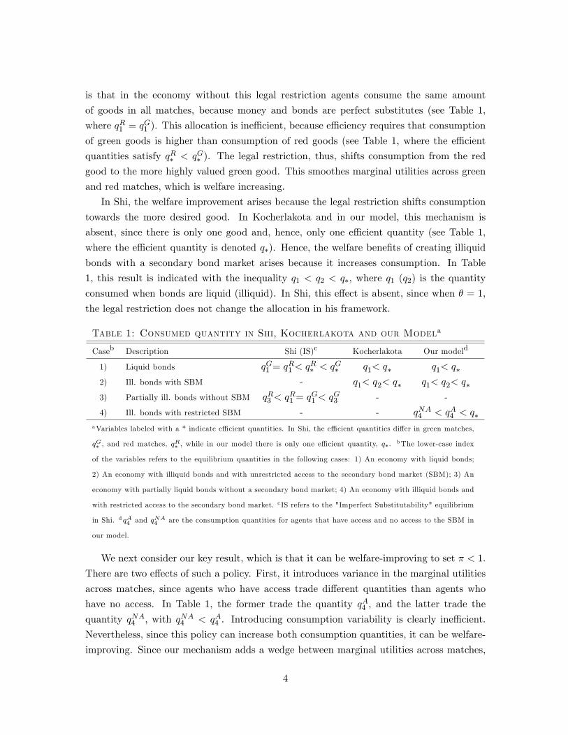
is that in the economy without this legal restriction agents consume the same amount

of goods in all matches, because money and bonds are perfect substitutes (see Table 1,

where qR1 = qG1 ). This allocation is ine¢ cient, because e¢ ciency requires that consumption

of green goods is higher than consumption of red goods (see Table 1, where the e¢ cient

quantities satisfy qR� < qG� ). The legal restriction, thus, shifts consumption from the red

good to the more highly valued green good. This smoothes marginal utilities across green

and red matches, which is welfare increasing.

In Shi, the welfare improvement arises because the legal restriction shifts consumption

towards the more desired good. In Kocherlakota and in our model, this mechanism is

absent, since there is only one good and, hence, only one e¢ cient quantity (see Table 1,

where the e¢ cient quantity is denoted q�). Hence, the welfare bene�ts of creating illiquid

bonds with a secondary bond market arises because it increases consumption. In Table

1, this result is indicated with the inequality q1 < q2 < q�, where q1 (q2) is the quantity

consumed when bonds are liquid (illiquid). In Shi, this e¤ect is absent, since when � = 1,

the legal restriction does not change the allocation in his framework.

Table 1: Consumed quantity in Shi, Kocherlakota and our Modela

Caseb Description Shi (IS)c Kocherlakota Our modeld

1) Liquid bonds qG1 = qR1 < q

R� < q

G� q1< q� q1< q�

2) Ill. bonds with SBM - q1< q2< q� q1< q2< q�3) Partially ill. bonds without SBM qR3 < q

R1 = q

G1 < q

G3 - -

4) Ill. bonds with restricted SBM - - qNA4 < qA4 < q�aVariables labeled with a * indicate e¢ cient quantities. In Shi, the e¢ cient quantities di¤er in green matches,

qG� , and red matches, qR� , while in our model there is only one e¢ cient quantity, q�.

bThe lower-case index

of the variables refers to the equilibrium quantities in the following cases: 1) An economy with liquid bonds;

2) An economy with illiquid bonds and with unrestricted access to the secondary bond market (SBM); 3) An

economy with partially liquid bonds without a secondary bond market; 4) An economy with illiquid bonds and

with restricted access to the secondary bond market. c IS refers to the "Imperfect Substitutability" equilibrium

in Shi. d qA4 and qNA4 are the consumption quantities for agents that have access and no access to the SBM in

our model.

We next consider our key result, which is that it can be welfare-improving to set � < 1.

There are two e¤ects of such a policy. First, it introduces variance in the marginal utilities

across matches, since agents who have access trade di¤erent quantities than agents who

have no access. In Table 1, the former trade the quantity qA4 , and the latter trade the

quantity qNA4 ; with qNA4 < qA4 . Introducing consumption variability is clearly ine¢ cient.

Nevertheless, since this policy can increase both consumption quantities, it can be welfare-

improving. Since our mechanism adds a wedge between marginal utilities across matches,

4

while Shi�s mechanism reduces such a wedge, it should be clear that our mechanism of

reducing access to the secondary bond market is very di¤erent from Shi�s legal restriction

model.

Our paper is also related to the macroeconomic literature that studies the implications

of pecuniary externalities for welfare (e.g., Caballero and Krishnamurthy, 2003; Lorenzoni,

2008; Bianchi and Mendoza, 2011; Jeanne and Korinek, 2012; Korinek, 2012). In this lit-

erature, the fundamental friction is limited commitment; i.e., agents have a limited ability

to commit to future repayments. Due to this friction, borrowing requires collateral, and

a pecuniary externality arises, because agents do not take into account how their borrow-

ing decisions a¤ect collateral prices, and through them the borrowing constraints of other

agents. As a consequence, the equilibrium is characterized by overborrowing, which is

de�ned as "the di¤erence between the amount of credit that an agent obtains acting atom-

istically in an environment with a given set of credit frictions, and the amount obtained by

a social planner who faces the same frictions but internalizes the general-equilibrium e¤ects

of its borrowing decisions" (see Bianchi and Mendoza, 2011, p.1).8

This pecuniary externality e¤ect has been used to study credit booms and busts. In a

model with competitive �nancial contracts and aggregate shocks, Lorenzoni (2008) identi-

�es excessive borrowing ex-ante and excessive volatility ex-post. In Bianchi and Mendoza

(2011), cyclical dynamics lead to a period of credit expansion up to the point where the

collateral constraint becomes binding, followed by sharp decreases in credit, asset prices and

macroeconomic aggregates (see also Mendoza and Smith, 2006; Mendoza, 2010). Jeanne

and Korinek (2012) study the optimal policy involved in credit booms and busts. They

�nd that it is optimal to impose cyclical taxes to prevent agents from excessive borrowing.

They emphasize that the level of the tax be adjusted for the vulnerability of each sector in

the economy.

In all of these papers, agents do not internalize the e¤ect of �re-sales on the value of

other agents�assets, and, therefore, they overborrow ex-ante. Our paper di¤ers from this

literature, because it is not a model of crisis: there are neither aggregate shocks nor multiple

steady-state equilibria. The pecuniary externality is present in "normal" times; i.e., in the

unique steady state equilibrium.9 Second, we propose a novel policy response to internalize

8Related to this literature are studies on �nancial accelerators (e.g., Bernanke and Gertler, 1989; Kiyotakiand Moore, 1997) or endogenous borrowing constraints (e.g, Kehoe and Levine, 1993; Berentsen, Camera,and Waller, 2007).

9Rojas-Breu (2013) also identi�es a pecuniary externality that is present in the steady state equilibrium.In her model, some agents use credit cards and some �at money to acquire consumption goods. She showsthat restricting the use of credit cards can be welfare improving. The intuition for this result is thatmarginally increasing the fraction of agents that use credit cards can have a general equilibrium e¤ect onthe price level, which makes the agents that have no credit card worse o¤. This e¤ect can be so strong thatoverall welfare decreases. In contrast to our model, in her model restricting the use of credit cards is a localoptimum only, since it would be optimal to endow all agents with credit cards.

5

the pecuniary externality by showing that reducing the frequency of trading can be optimal.

In contrast, Jeanne and Korinek (2012) propose a Pigouvian tax on borrowing and Bianchi

(2011) proposes a tax on debt to internalize the pecuniary externality.

3 The Model

Time is discrete, and in each period there are three markets which open sequentially.10

In the �rst market, agents trade money for nominal bonds. We refer to this market as

the secondary bond market. In the second market, agents produce or consume market-2

goods. We refer to this market as the goods market. In the third market, agents consume

and produce market-3 goods, receive money for maturing bonds, and acquire newly issued

bonds. We refer to this market as the primary bond market. All goods are nonstorable,

which means that they cannot be carried from one market to the next.

There is a [0; 1] continuum of in�nitely lived agents. At the beginning of each period,

agents receive two idiosyncratic i.i.d. shocks: a preference shock and an entry shock. The

preference shock determines whether an agent can produce or consume market-2 goods.

With probability 1 � n an agent can consume but not produce, and with probability nhe can produce but not consume. Consumers in the goods market are called buyers, and

producers are called sellers. The entry shock determines whether agents can participate

in the secondary bond market. With probability � they can, and with probability 1 � �they cannot. Agents who participate in the secondary bond market are called active, while

agents who do not are called passive. For active agents, trading in the secondary bond

market is frictionless.

In the goods market, agents meet at random in bilateral meetings. We represent trading

frictions by using a reduced-form matching function, �M (n; 1� n), where �M speci�es

the number of trade matches in a period and the parameter � is a scaling variable, which

determines the e¢ ciency of the matching process (see e.g., Rocheteau and Weill, 2011). We

assume that the matching function has constant returns to scale, and is continuous and

increasing with respect to each of its arguments. Let � (n) = �M (n; 1� n) (1 � n)�1 bethe probability that a buyer meets a seller. The probability that a seller meets a buyer

is denoted by �s (n) = � (n) (1� n)n�1. In what follows, to economize on notation, wesuppress the argument n, and refer to these probabilities as � and �s, respectively.

In the goods market, buyers get utility u (q) from consuming q units of market-2 goods,

where u0 (q) ;�u00 (q) > 0, u0 (0) =1, and u0 (1) = 0. Sellers incur the utility cost c(q) = q10Our basic framework is the divisible money model developed in Lagos and Wright (2005). This model

is useful, because it allows us to introduce heterogeneous preferences while still keeping the distribution ofasset holdings analytically tractable. The main departure from Lagos and Wright (2005) is that we add asecondary bond market.

6

from producing q units of market-2 goods.11

As in Lagos and Wright (2005), we impose assumptions that yield a degenerate distri-

bution of portfolios at the beginning of the secondary bond market. That is, we assume

that trading in the primary bond market is frictionless, that all agents can produce and

consume market-3 goods, and that the production technology is linear such that h units of

time produce h units of market-3 goods. The utility of consuming x units of goods is U(x),

where U 0 (x) ;�U 00 (x) > 0; U 0 (0) =1, and U 0 (1) = 0.Finally, agents discount between, but not within, periods. The discount factor between

two consecutive periods is � = 1=(1 + r); where r > 0 is the real interest rate.

3.1 First-best allocation

For a benchmark, it is useful to derive the planner allocation. The planner treats all agents

symmetrically. His optimization problem is

W = maxh;x;q

[� (1� n)u(q)� �snq] + U(x)� h; (1)

subject to the feasibility constraint h � x. The e¢ cient allocation satis�es U 0(x�) = 1,

u0(q�) = 1, and h� = x�. These are the quantities chosen by a social planner who dictates

consumption and production.12

3.2 Pricing mechanism

In what follows, we study the allocations that are attainable in a market economy. To

this end, we assume that the primary and secondary bond markets are characterized by

perfect competition. In contrast, we will investigate several pricing mechanism for the goods

market. The baseline case is random matching and generalized Nash bargaining. However,

we will also study random matching with Kalai bargaining, price-taking and competitive

search. We are in particular interested in how the di¤erent pricing mechanisms a¤ect the

portfolio choices of the agents in the primary and the secondary bond markets.

3.3 Money and bonds

The description of the environment in this subsection closely follows Berentsen and Waller

(2011).13 There are two perfectly divisible and storable �nancial assets: money and one-

11We assume a linear utility cost for ease of exposition. It is a simple generalization to allow for a moregeneral convex disutility cost.12Since our planner can dictate quantities, there is no need for either money or bonds to achieve the

�rst-best allocation.13However, the questions investigated in Berentsen and Waller (2011) are di¤erent to the questions studied

in this paper (see the literature review).

7

period, nominal discount bonds. Both are intrinsically useless, since they are neither ar-

guments of any utility function nor are they arguments of any production function. Both

assets are issued by the central bank in the last market. Bonds are payable to the bearer

and default free. One bond pays o¤ one unit of currency in the last market of the following

period.

At the beginning of a period, after the idiosyncratic shocks are revealed, agents can

trade bonds and money in the perfectly competitive secondary bond market. The central

bank acts as the intermediary for all bond trades by recording purchases and sales of bonds.

Bonds are book-keeping entries �no physical object exists. This implies that agents are not

anonymous to the central bank. Nevertheless, despite having a record-keeping technology

over bond trades, the central bank has no record-keeping technology over goods trades.

Since agents are anonymous and cannot commit, a buyer�s promise in the goods market to

deliver bonds to a seller in the primary bond market is not credible.

Since bonds are intangible objects, they cannot be used as a medium of exchange in

the goods market: hence they are illiquid. It has been shown in Kocherlakota (2003),

Andolfatto (2011), and Berentsen and Waller (2011) that in similar environments to the

one studied here, it is optimal that bonds are illiquid. All these papers assume unrestricted

access to bond markets. One of our contributions to this literature is to show that it is not

only optimal that bonds are illiquid, but that it can be optimal to reduce their liquidity

further by restricting access to bond markets.

To motivate a role for �at money, search models of money typically impose three as-

sumptions on the exchange process (Shi 2008):14 a double coincidence problem, anonymity,

and costly communication. First, our preference structure creates a single-coincidence prob-

lem in the goods market, since buyers do not have a good desired by sellers. Second, agents

in the goods market are anonymous, which rules out trade credit between individual buyers

and sellers. Third, there is no public communication of individual trading outcomes (public

memory), which, in turn, eliminates the use of social punishments in support of gift-giving

equilibria. The combination of these frictions implies that sellers require immediate com-

pensation from buyers. In short, there must be immediate settlement with some durable

asset, and money is the only such durable asset. These are the micro-founded frictions that

make money essential for trade in the goods market. In contrast, in the last market all

agents can produce for their own consumption or use money balances acquired earlier. In

this market, money is not essential for trade.15

DenoteMt as the per capita money stock and Bt as the per capita stock of newly issued

14See also Araujo (2004), Kocherlakota (1998), Wallace (2001), and Aliprantis, Camera and Puzzello(2007) for discussions of what makes money essential.15One can think of agents as being able to barter perfectly in this market. Obviously in such an environ-

ment, money is not needed.

8

bonds at the end of period t. Then Mt�1 (Bt�1) is the beginning-of-period money (bond)

stock in period t. Let �t denote the price of bonds in the primary bond market. Then, the

change in the money stock in period t is given by

Mt �Mt�1 = � tMt�1 +Bt�1 � �tBt: (2)

The change in the money supply at time t is given by three components: a lump-sum money

transfer (T = � tMt�1); the money created to redeem Bt�1 units of bonds; and the money

withdrawal from selling Bt units of bonds at the price �t. We assume there are positive

initial stocks of money M0 and bonds B0, with B0M0

> n1�n . For � t < 0, the government

must be able to extract money via lump-sum taxes from the economy.

4 Agent�s Decisions

For notational simplicity, the time subscript t is omitted when understood. Next-period

variables are indexed by +1, and previous-period variables are indexed by �1. In whatfollows, we look at a representative period t and work backwards, from the primary bond

market (the last market) to the secondary bond market (the �rst market).

4.1 Primary bond market

In the primary bond market, agents can consume and produce market-3 goods. Further-

more, they receive money for maturing bonds, buy newly issued bonds, adjust their money

balances by trading money for goods, and receive the lump-sum money transfer T . An

agent entering the primary bond market with m units of money and b units of bonds has

the indirect utility function V3(m; b). An agent�s decision problem in the primary bond

market is

V3(m; b) = maxx;h;m+1;b+1

[U(x)� h+ �V1(m+1; b+1)] ; (3)

subject to

x+ �m+1 + ��b+1 = h+ �m+ �b+ �T; (4)

where � is the price of money in terms of market-3 goods. The �rst-order conditions with

respect to m+1; b+1 and x are U 0(x) = 1, and

�@V1@m+1

= ��1�@V1@b+1

= �; (5)

where the term �@V1=@m+1 (�@V1=@b+1) is the marginal bene�t of taking one additional

unit of money (bonds) into the next period, and � (��) is the marginal cost of doing so.

9

Due to the quasi-linearity of preferences, the choices of b+1 and m+1 are independent of b

and m. It is straightforward to show that all agents exit the primary bond market with the

same portfolio of bonds and money. The envelope conditions are

@V3@m

=@V3@b

= �: (6)

According to (6), the marginal value of money and bonds at the beginning of the primary

bond market is equal to the price of money in terms of market-3 goods. Note that equations

(6) imply that the value function V3 is linear in m and b.

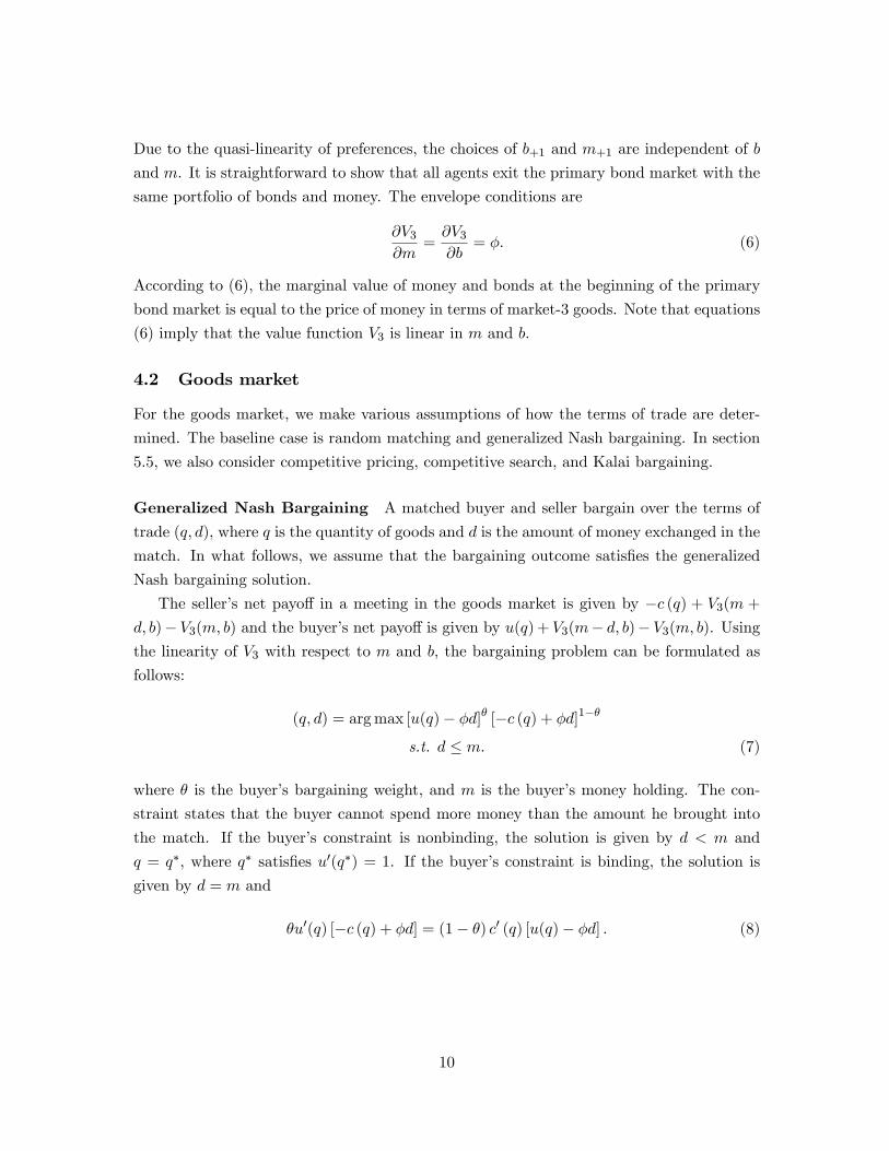
4.2 Goods market

For the goods market, we make various assumptions of how the terms of trade are deter-

mined. The baseline case is random matching and generalized Nash bargaining. In section

5.5, we also consider competitive pricing, competitive search, and Kalai bargaining.

Generalized Nash Bargaining A matched buyer and seller bargain over the terms of

trade (q; d), where q is the quantity of goods and d is the amount of money exchanged in the

match. In what follows, we assume that the bargaining outcome satis�es the generalized

Nash bargaining solution.

The seller�s net payo¤ in a meeting in the goods market is given by �c (q) + V3(m +

d; b)� V3(m; b) and the buyer�s net payo¤ is given by u(q) + V3(m� d; b)� V3(m; b). Usingthe linearity of V3 with respect to m and b, the bargaining problem can be formulated as

follows:

(q; d) = argmax [u(q)� �d]� [�c (q) + �d]1��

s.t. d � m: (7)

where � is the buyer�s bargaining weight, and m is the buyer�s money holding. The con-

straint states that the buyer cannot spend more money than the amount he brought into

the match. If the buyer�s constraint is nonbinding, the solution is given by d < m and

q = q�, where q� satis�es u0(q�) = 1. If the buyer�s constraint is binding, the solution is

given by d = m and

�u0(q) [�c (q) + �d] = (1� �) c0 (q) [u(q)� �d] : (8)

10

This latter condition can be written as follows:

�m = z (q) � �c (q)u0(q) + (1� �)u(q)c0 (q)�u0(q) + (1� �) c0 (q) : (9)

This is by now a routine derivation of the Nash bargaining solution in a Lagos and Wright-

type model. More details can be found in Lagos and Wright (2005) or Nosal and Rocheteau

(2011).

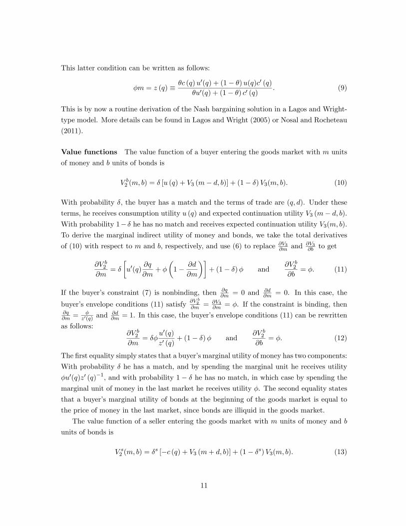
Value functions The value function of a buyer entering the goods market with m units

of money and b units of bonds is

V b2 (m; b) = � [u (q) + V3 (m� d; b)] + (1� �)V3(m; b): (10)

With probability �, the buyer has a match and the terms of trade are (q; d). Under these

terms, he receives consumption utility u (q) and expected continuation utility V3 (m� d; b).With probability 1� � he has no match and receives expected continuation utility V3(m; b):To derive the marginal indirect utility of money and bonds, we take the total derivatives

of (10) with respect to m and b, respectively, and use (6) to replace @V3@m and @V3

@b to get

@V b2@m

= �

�u0(q)

@q

@m+ �

�1� @d

@m

��+ (1� �)� and

@V b2@b

= �: (11)

If the buyer�s constraint (7) is nonbinding, then @q@m = 0 and @d

@m = 0. In this case, the

buyer�s envelope conditions (11) satisfy @V b2@m = @V3

@m = �. If the constraint is binding, then@q@m =

�z0(q) and

@d@m = 1. In this case, the buyer�s envelope conditions (11) can be rewritten

as follows:@V b2@m

= ��u0(q)

z0 (q)+ (1� �)� and

@V b2@b

= �: (12)

The �rst equality simply states that a buyer�s marginal utility of money has two components:

With probability � he has a match, and by spending the marginal unit he receives utility

�u0(q)z0 (q)�1, and with probability 1� � he has no match, in which case by spending themarginal unit of money in the last market he receives utility �. The second equality states

that a buyer�s marginal utility of bonds at the beginning of the goods market is equal to

the price of money in the last market, since bonds are illiquid in the goods market.

The value function of a seller entering the goods market with m units of money and b

units of bonds is

V s2 (m; b) = �s [�c (q) + V3 (m+ d; b)] + (1� �s)V3(m; b): (13)

11

The interpretation of (13) is similar to the interpretation of (10) and is omitted. Taking

the total derivative of (13) with respect to m and b, respectively, and using (6) to replace@V3@m and @V3

@b , yields the seller�s envelope conditions:

@V s2@m

=@V s2@b

= �: (14)

These conditions simply state that a seller�s marginal utility of money and bonds at the

beginning of the goods market are equal to the price of money in the last market. The

reason is that a seller has no use for these two assets in the goods market.

4.3 Secondary bond market

Let (m̂; b̂) denote the portfolio of an active agent after trading in the secondary bond market,

and let ' denote the price of bonds in terms of money in the secondary bond market. Then,

an active agent�s budget constraint satis�es

�m+ '�b � �m̂+ '�b̂: (15)

The left-hand side of (15) is the sum of the real values of money and bonds with which the

agent enters the secondary bond market, and the right-hand side is the real value of the

portfolio with which the agent leaves the secondary bond market.

Trading is further constrained by two short-selling constraints: Active agents cannot

sell more bonds, and they cannot spend more money, than the amount they carry from the

previous period: that is

m̂ � 0; b̂ � 0: (16)

Let V j1 (m; b) denote the value functions of an active buyer (j = b) or an active seller (j = s).

Then, an active agent�s decision problem is

V j1 (m; b) = maxm̂;b̂

V j2 (m̂; b̂) s.t. (15) and (16).

The secondary bond market�s �rst-order conditions for active agents are

@V j2@m̂

= ��j � �jm; and@V j2@b̂

= '��j � �jb; (17)

where, for j = b; s, �j are the Lagrange multipliers on (15), and �jm and �jb are the Lagrange

multipliers on (16).

Finally, let V1(m; b) denote the expected value for an agent who enters the secondary

bond market with m units of money and b units of bonds before the idiosyncratic shocks

12

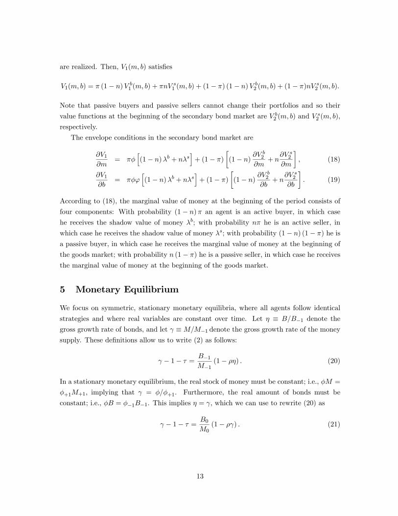
are realized. Then, V1(m; b) satis�es

V1(m; b) = � (1� n)V b1 (m; b) + �nV s1 (m; b) + (1� �) (1� n)V b2 (m; b) + (1� �)nV s2 (m; b):

Note that passive buyers and passive sellers cannot change their portfolios and so their

value functions at the beginning of the secondary bond market are V b2 (m; b) and Vs2 (m; b),

respectively.

The envelope conditions in the secondary bond market are

@V1@m

= ��h(1� n)�b + n�s

i+ (1� �)

�(1� n) @V

b2

@m+ n

@V s2@m

�; (18)

@V1@b

= ��'h(1� n)�b + n�s

i+ (1� �)

�(1� n) @V

b2

@b+ n

@V s2@b

�: (19)

According to (18), the marginal value of money at the beginning of the period consists of

four components: With probability (1� n)� an agent is an active buyer, in which casehe receives the shadow value of money �b; with probability n� he is an active seller, in

which case he receives the shadow value of money �s; with probability (1� n) (1� �) he isa passive buyer, in which case he receives the marginal value of money at the beginning of

the goods market; with probability n (1� �) he is a passive seller, in which case he receivesthe marginal value of money at the beginning of the goods market.

5 Monetary Equilibrium

We focus on symmetric, stationary monetary equilibria, where all agents follow identical

strategies and where real variables are constant over time. Let � � B=B�1 denote the

gross growth rate of bonds, and let �M=M�1 denote the gross growth rate of the money

supply. These de�nitions allow us to write (2) as follows:

� 1� � = B�1M�1

(1� ��) : (20)

In a stationary monetary equilibrium, the real stock of money must be constant; i.e., �M =

�+1M+1; implying that = �=�+1. Furthermore, the real amount of bonds must be

constant; i.e., �B = ��1B�1. This implies � = , which we can use to rewrite (20) as

� 1� � = B0M0

(1� � ) : (21)

13

The model has three types of stationary monetary equilibria. In what follows, we charac-

terize these types of equilibria. To simplify notation, let

(q) � � u0(q)

z0 (q)+ 1� �: (22)

Furthermore, in what follows we assume that (q) is decreasing in q. This assumption

guarantees that our stationary monetary equilibrium derived below is unique.16

5.1 Type I equilibrium

In a type I equilibrium, an active buyer�s bond constraint in the secondary bond market

does not bind, and a seller�s cash constraint in the secondary bond market does not bind. In

the Appendix, we show that a type I equilibrium can be characterized by the four equations

stated in Lemma 1.

Lemma 1 A type I equilibrium is a time-independent list fq; q̂; �; 'g satisfying

' = 1; (23)

�= � + (1� �) [(1� n) (q) + n] ; (24)

� =�

; (25)

u0 (q̂) = z0 (q̂) : (26)

In a type I equilibrium, the seller�s cash constraint in the secondary bond market does

not bind. This can only be the case if he is indi¤erent between holding money or bonds,

which requires ' = 1; i.e., that equation (23) holds. According to (25), the price of bonds

in the primary bond market is equal to its fundamental value �= . The reason for this

result is that bonds in the primary market attain no liquidity premium (see our discussion

below), since an active buyer�s constraint on bond holdings in the secondary bond market

does not bind.

According to (26), active buyers consume the quantity q̂ that satis�es u0 (q̂) = z0 (q̂).

If � < 1, then q̂ < q�; so they consume the ine¢ cient quantity even as � ! . If � = 1,

then q̂ = q�; and they consume the e¢ cient quantity. From (24), the consumed quantity

for passive buyers, q, is ine¢ cient for all �.

16Lagos and Wright (2005, p. 472) investigate under which conditions u0(q)z0(q) is decreasing in q. They argue

that u0(q)z0(q) "is monotone if � � 1, or if c (q) is linear and u0 (q) log-concave." For a comprehensive study of

existence and uniqueness of equilibrium in the Lagos and Wright framework see Wright (2010).

14

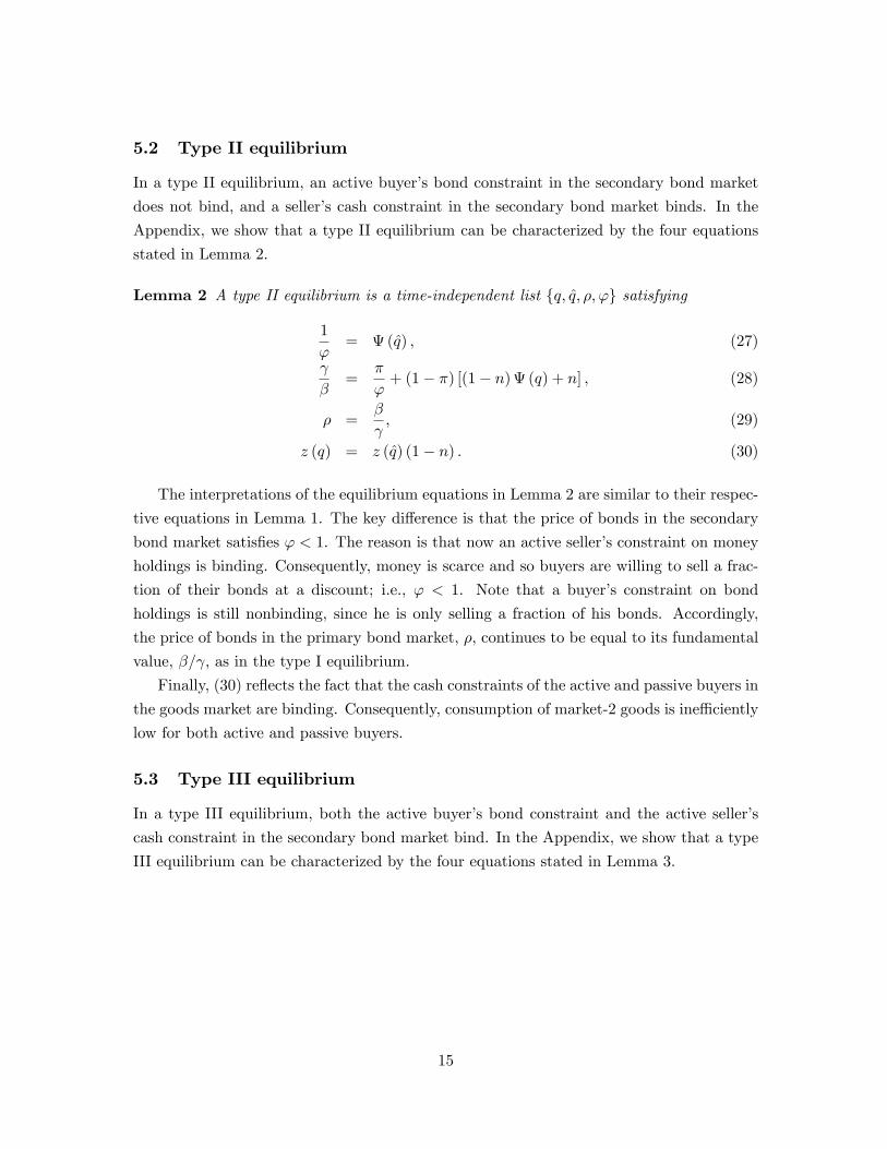
5.2 Type II equilibrium

In a type II equilibrium, an active buyer�s bond constraint in the secondary bond market

does not bind, and a seller�s cash constraint in the secondary bond market binds. In the

Appendix, we show that a type II equilibrium can be characterized by the four equations

stated in Lemma 2.

Lemma 2 A type II equilibrium is a time-independent list fq; q̂; �; 'g satisfying

1

'= (q̂) ; (27)

�=

�

'+ (1� �) [(1� n) (q) + n] ; (28)

� =�

; (29)

z (q) = z (q̂) (1� n) : (30)

The interpretations of the equilibrium equations in Lemma 2 are similar to their respec-

tive equations in Lemma 1. The key di¤erence is that the price of bonds in the secondary

bond market satis�es ' < 1. The reason is that now an active seller�s constraint on money

holdings is binding. Consequently, money is scarce and so buyers are willing to sell a frac-

tion of their bonds at a discount; i.e., ' < 1. Note that a buyer�s constraint on bond

holdings is still nonbinding, since he is only selling a fraction of his bonds. Accordingly,

the price of bonds in the primary bond market, �, continues to be equal to its fundamental

value, �= , as in the type I equilibrium.

Finally, (30) re�ects the fact that the cash constraints of the active and passive buyers in

the goods market are binding. Consequently, consumption of market-2 goods is ine¢ ciently

low for both active and passive buyers.

5.3 Type III equilibrium

In a type III equilibrium, both the active buyer�s bond constraint and the active seller�s

cash constraint in the secondary bond market bind. In the Appendix, we show that a type

III equilibrium can be characterized by the four equations stated in Lemma 3.

15

Lemma 3 A type III equilibrium is a time-independent list fq; q̂; �; 'g satisfying

1

'=B0M0

1� nn

; (31)

�= � [(1� n) (q̂) + n='] + (1� �) [(1� n) (q) + n] ; (32)

� =�

f1 + � (1� n) ['(q̂)� 1]g ; (33)

z (q) = z (q̂) (1� n): (34)

According to (33), the price of bonds in the primary bond market � includes two compo-

nents: the fundamental value of bonds, �= , and the liquidity premium, � � (1� n) ['(q̂)� 1].The liquidity premium is increasing in � and equal to zero at � = 0. In contrast, there is

no liquidity premium in the type I and type II equilibria, since an active buyer�s constraint

on bond holdings is not binding.

Furthermore, from (31), note that the price of bonds in the secondary bond market, ',

is constant (in contrast to the type II equilibrium). The reason is that in Lemma 3, ' is

obtained from the secondary bond market budget constraint, (15). In contrast, in Lemmas

1 and 2 it is obtained from the secondary bond market �rst-order conditions (17). Finally,

(34) has the same interpretation as (30).

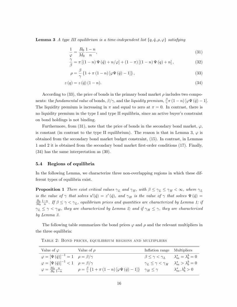
5.4 Regions of equilibria

In the following Lemma, we characterize three non-overlapping regions in which these dif-

ferent types of equilibria exist.

Proposition 1 There exist critical values L and H , with � � L � H < 1, where Lis the value of that solves u0(q̂) = z0 (q̂), and H is the value of that solves (q̂) =B0M0

1�nn . If � � < L, equilibrium prices and quantities are characterized by Lemma 1; if

L � < H , they are characterized by Lemma 2; and if H � , they are characterized

by Lemma 3.

The following table summarizes the bond prices ' and � and the relevant multipliers in

the three equilibria:

Table 2: Bond prices, equilibrium regions and multipliers

Value of ' Value of � In�ation range Multipliers

' = [ (q̂)]�1 = 1 � = �= � � < L �sm = �bb = 0

' = [ (q̂)]�1 < 1 � = �= L � < H �sm > �bb = 0

' = M0B0

n1�n � = �

f1 + � (1� n) ['(q̂)� 1]g H � �sm; �bb > 0

16

In the type I and II equilibria (� � < H), the constraint on bond holdings of activebuyers does not bind (�bb = 0) in the secondary bond market. This implies that the return

on bonds in the secondary bond market, 1=', has to be equal to the expected return on

money, (q̂). It also implies that the price of bonds in the primary bond market, �,

must equal the fundamental value of bonds, �= . The economics underlying this result are

straightforward. Since active buyers do not sell all their bonds for money in the secondary

bond market, bonds in the primary bond market have no liquidity premium, and so the

Fisher equation holds; i.e., 1=� = =�.17

In contrast, in the type III equilibrium, the constraint on bond holdings of active buyers

binds in the secondary bond market. Consequently, bonds attain a liquidity premium, and

the Fisher equation does not hold; i.e., 1=� < =�.18

π = 1

ρ = φ

1

β = γL

Type I Type II Type III

γH γ

φ

ρ

1

γγL γHβ

π < 1

Type I Type II Type III

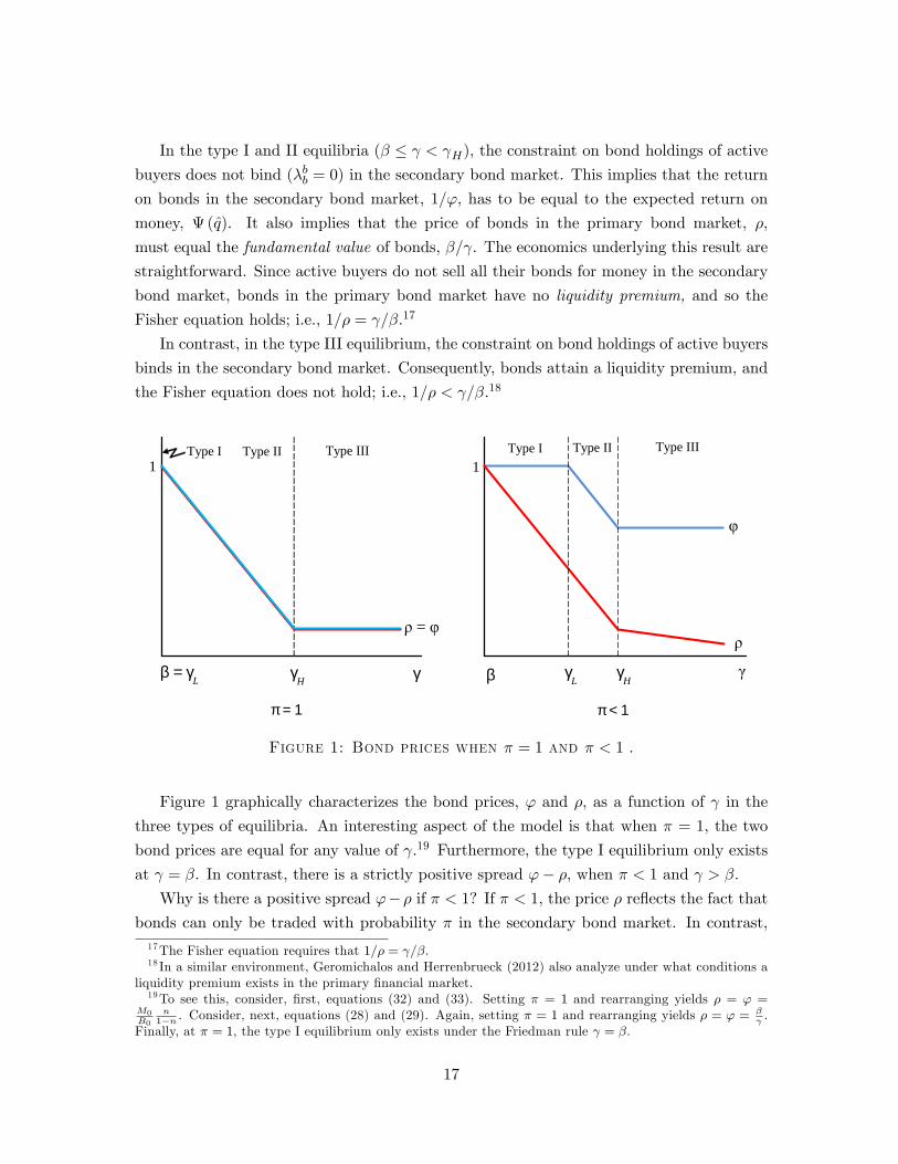
Figure 1: Bond prices when � = 1 and � < 1 .

Figure 1 graphically characterizes the bond prices, ' and �, as a function of in the

three types of equilibria. An interesting aspect of the model is that when � = 1, the two

bond prices are equal for any value of .19 Furthermore, the type I equilibrium only exists

at = �. In contrast, there is a strictly positive spread '� �, when � < 1 and > �.Why is there a positive spread '�� if � < 1? If � < 1, the price � re�ects the fact that

bonds can only be traded with probability � in the secondary bond market. In contrast,17The Fisher equation requires that 1=� = =�.18 In a similar environment, Geromichalos and Herrenbrueck (2012) also analyze under what conditions a

liquidity premium exists in the primary �nancial market.19To see this, consider, �rst, equations (32) and (33). Setting � = 1 and rearranging yields � = ' =

M0B0

n1�n . Consider, next, equations (28) and (29). Again, setting � = 1 and rearranging yields � = ' =

� .

Finally, at � = 1, the type I equilibrium only exists under the Friedman rule = �.

17

the price ' re�ects the fact that active agents can trade bonds with probability 1 in the

secondary bond market. Thus, the positive spread is because the bonds in the secondary

bond market have a higher liquidity premium than the bonds in the primary bond market.

As can be seen in Figure 1, when, � < 1, the price of bonds in the secondary bond

market, ', is constant and equal to 1 in the type I equilibrium; it is decreasing in the type

II equilibrium; and it is constant in the type III equilibrium. The price of bonds in the

primary bond market, �, follows a di¤erent pattern. In the type I and type II equilibrium,

it is equal to the fundamental value of bonds, �= , whereas in the type III equilibrium, it

contains a liquidity premium. The lower � in the type III equilibrium is, the larger is the

di¤erence between ' and �.

5.5 Other pricing mechanisms

Here we discuss how the key equations change when we assume one of the other pric-

ing mechanisms mentioned above. Using the Kalai bargaining solution is straightforward.

Competitive pricing and competitive search are a bit more involved, and we present the

derivations in the Appendix.

Kalai bargaining The Nash bargaining solution is non-monotonic (see Aruoba, Ro-

cheteau, and Waller; 2007). In contrast, the Kalai bargaining solution, also referred to

as proportional bargaining (Kalai; 1977), is monotonic and because of this property it is

increasingly used in monetary economics.20 It can be formalized as follows:

(q; d) = argmaxu(q)� �d

s.t. u(q)� �d = � [u(q)� c (q)] and d � m:

When the buyer�s cash constraint is binding, the solution is d = m and

�m = zK (q) � �c (q) + (1� �)u(q); (35)

where the superscript K refers to Kalai bargaining. When the buyer�s constraint (7) is

binding, the Kalai bargaining solution di¤ers from the Nash bargaining solution unless

� = 0 or � = 1. When the constraint is nonbinding, Nash bargaining and Kalai bargaining

yield the same solution.

20The Kalai bargaining solution is discussed in Aruoba, Rocheteau, and Waller (2007) and is used, forexample, in Rocheteau and Wright (2010), Lester, Postlewaite, and Wright (2012), He, Wright, and Zhu(2012), and Trejos and Wright (2012). For a textbook treatment of the Kalai bargaining solution see Nosaland Rocheteau (2011).

18

It is straightforward to study the model under Kalai bargaining. One only needs to

replace z (q) with zK (q) in Lemmas 1-3.

Competitive search Let � (n) be the seller�s contribution to the matching process; i.e.,

the elasticity of the matching function with respect to the measures of sellers. In the

Appendix, we show that under competitive search, the terms of trade satisfy

�m = zP (q) , where (36)

zP (q) � [1� � (n)] c (q)u0(q) + � (n)u(q)c0 (q)[1� � (n)]u0(q) + � (n) c0 (q) :

It is straightforward to study the model under competitive search. One only needs to

replace z (q) with zP (q) in Lemmas 1-3.

Competitive pricing Competitive pricing di¤ers from random matching and bargaining

along two dimensions. Obviously, there is no random matching, meaning that agents trade

with certainty, since in competitive equilibrium buyers and sellers trade against the market.

To make the results comparable, however, we assume that buyers and sellers can enter the

goods market only probabilistically with probability � and �s, respectively. The bene�t of

this assumption is that all di¤erences in results are due to the pricing mechanism since the

number of trades is equal under all pricing protocols.

The second di¤erence is that there is no bargaining; instead, the competitive price

adjusts to equate aggregate demand and aggregate supply. The market clearing condition

for the goods market is

�(1� n) [�q̂ + (1� �)q] = �snqs; (37)

where q̂ (q) is the quantity consumed by a buyer who has (no) access to the secondary bond

market.

In the Appendix, we show that competitive pricing yields the same allocation as random

matching and bargaining if the buyers have all the bargaining power; i.e., � = 1. In

particular, the terms of trade satisfy21

zC (q) � q: (38)

It is then straightforward to study the model under competitive pricing. One only needs to

replace z (q) with zC (q) in Lemmas 1-3.

21 In general, the condition is zC (qs; q) � c0 (qs) q, where qs is a seller�s production. With a linear costfunction, c (qs) = qs, the condition reduces to zC (q) � q.

19

6 Optimal Participation

In this section, we discuss the following. First, we show that if agents have a choice to

participate in the secondary bond market, they strictly prefer to do so. Second, we show

that such a participation choice involves a negative pecuniary externality. Third, we discuss

optimal secondary market participation.

6.1 Endogenous participation

So far, we have assumed that participation in the secondary bond market is determined by

the exogenous idiosyncratic participation shock �. Suppose instead that each agent has a

choice. Recall that V b1 (m; b) is the expected lifetime utility of a buyer at the beginning of

the secondary bond market, and V b2 (m; b) is the expected lifetime utility of a buyer at the

beginning of the goods market who had no access to the secondary bond market. Then, for

a buyer, it is optimal to participate if

V b1 (m; b) � V b2 (m; b):

Note that the exact experiment here is to keep all prices at their equilibrium values for a

given participation rate �, and, then, to ask the question, whether a single buyer would

prefer to enter the secondary bond market. The move of a single buyer from passive to

active does not change equilibrium prices.

Lemma 4 In any equilibrium, V b1 (m; b)� V b2 (m; b) � 0.

According to Lemma 4, a buyer is always better o¤when participating in the secondary

bond market. To develop an intuition for this result, note that, as shown in the proof of

Lemma 4,

V b1 (m; b)� V b2 (m; b) = u (q̂)� q̂ � [u (q)� q]� i (q̂ � q) ; (39)

where i = (1� ') =' is the nominal interest rate. A passive buyer�s period surplus is

u (q) � q, while an active buyer�s surplus is u (q̂) � q̂ � i (q̂ � q), where the term i (q̂ � q)measures the utility cost of selling bonds to �nance the di¤erence q̂� q � 0. The di¤erenceu (q̂)� q̂ � [u (q)� q] is strictly positive, while the term �i (q̂ � q) is negative. The reasonis that in any equilibrium q � q̂ � q�. Thus, the equilibrium interest rate cannot be too

large in order for (39) to be positive. In the proof of Lemma 4, we replace i in (39) for all

three types of equilibria and �nd that V b1 (m; b)� V b2 (m; b) > 0.We now turn to the sellers. For them, we also �nd that they are better o¤ when

participating in the secondary bond market.

20

Lemma 5 In any equilibrium, V s1 (m; b)� V s2 (m; b) � 0.

In the type I equilibrium, the nominal interest rate is i = 0. In this case, V s1 (m; b) =

V s2 (m; b). In the type II and type III equilibria, the nominal interest rate is i > 0: In this

case, the seller strictly prefers to enter, since V s1 (m; b) > Vs2 (m; b).

6.2 Optimal secondary bond market participation

Lemmas 4 and 5 show that if agents have a choice, they will participate in the secondary

bond market. In this section, we explain why restricting participation to the secondary

bond market can be welfare-improving. The reason is straightforward. The secondary

bond market provides insurance against the idiosyncratic liquidity shocks. At the end of a

period in the primary bond market, agents choose a portfolio of bonds and money. At this

point, they do not know yet whether they will be buyers or sellers in the following period.

At the beginning of the following period, this information is revealed, and they can use the

secondary bond market to readjust their portfolio of money and illiquid bonds.

From a welfare point of view, the bene�t of the secondary bond market is that it allocates

liquidity to the buyers and allows sellers to earn interest on their idle money holdings. The

drawback of this opportunity is that the secondary bond market reduces the incentive to

self-insure against the liquidity shocks. This lowers the demand for money in the primary

bond market, which depresses its value. This e¤ect can be so strong that it can be optimal

to restrict access to the secondary bond market. The basic mechanism can be seen from

the following welfare calculations.

The welfare function can be written as follows:

(1� �)W = (1� n) � f� [u(q̂)� q̂] + (1� �) [u(q)� q]g+ U(x�)� x�; (40)

where the term in the curly brackets is an agent�s expected period utility in the goods

market, and U(x�)� x� is the agent�s period utility in the primary bond market.Di¤erentiating (40) with respect to � yields

1� �(1� n) �

dWd�

= [u(q̂)� q̂]� [u(q)� q] (41)

+��u0(q̂)� 1

� dq̂d�+ (1� �)

�u0(q)� 1

� dqd�:

The contribution of the �rst two terms to the change in welfare is always positive, since in

any equilibrium q̂ � q (with strict inequality for > �). However, the derivatives dq̂d� and

dqd� can be negative, re�ecting the fact that increasing participation reduces the incentive

21

to self-insure against idiosyncratic liquidity risk.22 Reducing the incentive to self-insure

reduces the demand for money and hence its value, which then reduces the consumption

quantities q and q̂.

Whether restricting participation is welfare-improving depends on which of the two

e¤ects dominates. One can show that in the type I and in the type II equilibria it is always

optimal to set � = 1. In contrast, restricting participation in the type III equilibrium

can be welfare-improving. Whether it is depends on preferences and technology. In the

following, we calibrate the model to investigate whether restricting access to the secondary

bond market is optimal under reasonable parameter values.23

7 Quantitative Analysis

We choose a model period as one quarter. The functions u(q) and c(q) have the forms

u (q) = Aq1��=(1� �) and c(q) = q:

For the matching function, we follow Kiyotaki and Wright (1993) and choose

M(B;S) = BS=(B + S),

where B = 1 � n is the measure of buyers and S = n the measure of sellers in the goodsmarket. Therefore, the matching probability of a buyer in the goods market is simply given

by � = �M(B;S)=B = �n.

The parameters to be identi�ed are as follows: (i) preference parameters: (�;A; �);

(ii) technology parameters: (n; �); (iii) bargaining power: �; (iv) policy parameters: the

money growth rate and the bonds-to-money ratio B. Finally, we set � = 1 for all but onecalibration, where as a robustness check we choose � = 0:5.

To identify these parameters, we use US-data from the �rst quarter of 1960 to the

fourth quarter of 2010. All data sources are provided in the Appendix. Table 3 lists the

identi�cation restrictions and the identi�ed values of the parameters.

22A su¢ cient condition for these derivatives to be negative is that (q) = � u0(q)z0(q) + 1� � is decreasing in

q, which is an assumption throughout the paper.23 In an earlier version of the paper, we provided an analytical proof that if in�ation is su¢ ciently high, it

is optimal to restrict access to the secondary bond market for u(q) = ln (q) and perfect competition in thegoods market.

22

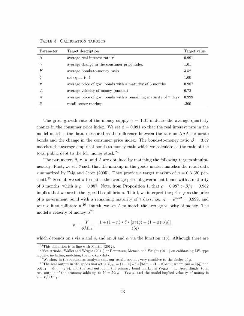
Table 3: Calibration targets

Parameter Target description Target value

� average real interest rate r 0.991

average change in the consumer price index 1.01

B average bonds-to-money ratio 3.52

� set equal to 1 1.00

� average price of gov. bonds with a maturity of 3 months 0.987

A average velocity of money (annual) 6.72

n average price of gov. bonds with a remaining maturity of 7 days 0.999

� retail sector markup .300

The gross growth rate of the money supply = 1:01 matches the average quarterly

change in the consumer price index. We set � = 0:991 so that the real interest rate in the

model matches the data, measured as the di¤erence between the rate on AAA corporate

bonds and the change in the consumer price index. The bonds-to-money ratio B = 3:52

matches the average empirical bonds-to-money ratio which we calculate as the ratio of the

total public debt to the M1 money stock.24

The parameters �, �, n, and A are obtained by matching the following targets simulta-

neously. First, we set � such that the markup in the goods market matches the retail data

summarized by Faig and Jerez (2005). They provide a target markup of � = 0:3 (30 per-

cent).25 Second, we set � to match the average price of government bonds with a maturity

of 3 months, which is � = 0:987. Note, from Proposition 1, that � = 0:987 > �= = 0:982

implies that we are in the type III equilibrium. Third, we interpret the price ' as the price

of a government bond with a remaining maturity of 7 days; i.e., ' = �4=52 = 0:999, and

we use it to calibrate n.26 Fourth, we set A to match the average velocity of money. The

model�s velocity of money is27

v =Y

�M�1=1 + (1� n) � � � [�z(q̂) + (1� �) z(q)]

z(q);

which depends on i via q and q̂, and on A and � via the function z(q). Although there are

24This de�nition is in line with Martin (2012).25See Aruoba, Waller and Wright (2011) or Berentsen, Menzio and Wright (2011) on calibrating LW-type

models, including matching the markup data.26We show in the robustness analysis that our results are not very sensitive to the choice of '.27The real output in the goods market is YGM = (1� n) � � � [��m̂+ (1� �)�m], where �m̂ = z(q̂) and

�M�1 = �m = z(q), and the real output in the primary bond market is YPBM = 1. Accordingly, totalreal output of the economy adds up to Y = YGM + YPBM ; and the model-implied velocity of money isv = Y=�M�1.

23

alternative ways to �t this relationship, we set A to match the average Y=�M�1, using M1

as our measure of money.

Our targets discussed above and summarized in Table 3 are su¢ cient to calibrate all but

one parameter, the elasticity of the utility function �. Berentsen, Menzio and Wright (2011)

estimate that � 2 (0:105; 0:211), depending on the calibration method. We, therefore, �rstpresent the calibration results for an average value of � = 0:15 and, then, show the e¤ects

of di¤erent values of � later on.28

7.1 Baseline results and robustness checks under Nash bargaining

Table 4 presents the results for the baseline calibration and four robustness checks under

generalized Nash bargaining. The robustness checks are de�ned as follows: In the calibra-

tion labeled "markup", we target a markup in the goods market of 40 percent instead of 30

percent; in the calibration labeled "high B", we target B = 4:5 instead of B = 3:5; in thecalibration labeled "high '", we target a remaining maturity of government bonds of 1 day

instead of 7 days; and in the calibration labeled "low �", we set � = 0:5 instead of � = 1.

28Most monetary models that calibrate variants of the Lagos and Wright (2005) framework, set � to matchthe elasticity of money demand with respect to the nominal interest rate. We cannot do this, because in ourframework the interest rate on � represents the yield on 3-month government bonds, while related studieswork with the AAA Moody�s corporate bond yield to calculate the elasticity of money demand. UsingUnited States data from 1960 to 2010, we obtain an empirical elasticity of money demand with respect tothe yield on 3-month government bonds of �gov = 0:05. The elasticity of money demand in our model isnegative by construction, which precludes the use of this target.

24

Table 4: Nash bargaininga

Description baseline markup high B high ' low �

A goods market utility weight 1.42 1.47 1.48 1.41 1.51

n number of sellers .778 .778 .818 .779 .778

� buyer�s bargaining share .387 .309 .416 .390 .495

� calibrated � .588 .550 .594 .574 .514

�� optimal �b .589 .548 .568 .555 .532

W� Wefare at calibrated � 18.551 19.381 18.934 18.192 9.258

W�� Wefare at � = �� 18.551 19.381 18.942 18.195 9.260

W1 Wefare at � = 1 17.150 17.496 16.929 16.571 8.321

sGM goods market size .315 .301 .310 .310 .144aTable 4 displays the calibrated values for the key parameters A, n and � for the value of � = 0:15.

It also displays the calibrated value of �, the optimal value of � (��) and the size of the goods

market (sGM ). Furthermore, the table also shows the numerical value of the welfare function

at the calibrated value of �, at the optimal value of � = ��, and at � = 1. b�� is calculated

numerically by searching for the welfare maximizing value of �, holding all other parameters at

their calibrated values.

Table 4 presents the key parameter values for the baseline calibration and the robustness

checks when � = 0:15. To address the question of whether there is too much trading in

the secondary bond market, we also calculate the optimal entry probability �� for each

case. It is calculated as follows. For each set of calibrated parameter values, we numerically

search for the value of � that maximizes ex-ante welfare, de�ned by (40). Furthermore, we

also provide the numerical value of the welfare function at the calibrated value of �, at the

optimal value of � = ��, and at � = 1.29

We �nd two key results. First, our calibrations always yield an entry probability �,

which is strictly below 1. Second, the optimal entry probability �� is below the calibrated

entry probability for a su¢ ciently high markup, a high bonds-to-money ratio, and a high

value of '. In contrast, under the baseline calibration and the calibration with a low

matching probability �, we �nd that the access to the secondary bond market should be

slightly increased in order to maximize ex-ante welfare.

In Table 4, we also provide the estimates of the model-implied goods market share on

total output, sGM = YGM=Y . Under Nash bargaining, the goods market share on total

29For the provided value of the welfare function we choose U(x) = x.

25

output is in the area of 31% for � = 1; and for a lower matching probability (� = 0:5) it

is in the area of 14%, which is in line with the estimates of Berentsen, Menzio and Wright

(2011) and related studies.

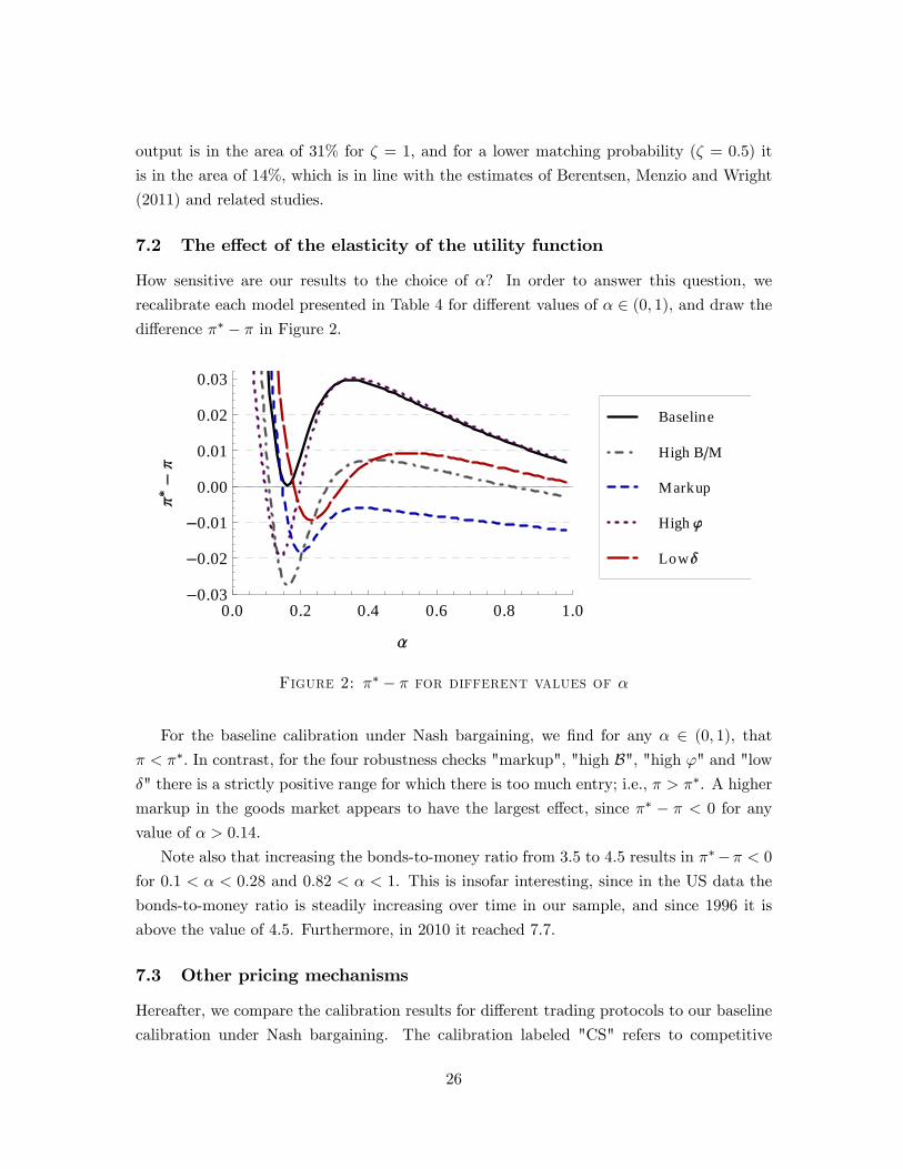
7.2 The e¤ect of the elasticity of the utility function

How sensitive are our results to the choice of �? In order to answer this question, we

recalibrate each model presented in Table 4 for di¤erent values of � 2 (0; 1), and draw thedi¤erence �� � � in Figure 2.

0.0 0.2 0.4 0.6 0.8 1.00.03

0.02

0.01

0.00

0.01

0.02

0.03

Low

High

Markup

High B M

Baseline

Figure 2: �� � � for different values of �

For the baseline calibration under Nash bargaining, we �nd for any � 2 (0; 1), that� < ��. In contrast, for the four robustness checks "markup", "high B", "high '" and "low�" there is a strictly positive range for which there is too much entry; i.e., � > ��. A higher

markup in the goods market appears to have the largest e¤ect, since �� � � < 0 for any

value of � > 0:14.

Note also that increasing the bonds-to-money ratio from 3:5 to 4:5 results in ���� < 0for 0:1 < � < 0:28 and 0:82 < � < 1. This is insofar interesting, since in the US data the

bonds-to-money ratio is steadily increasing over time in our sample, and since 1996 it is

above the value of 4:5. Furthermore, in 2010 it reached 7:7.

7.3 Other pricing mechanisms

Hereafter, we compare the calibration results for di¤erent trading protocols to our baseline

calibration under Nash bargaining. The calibration labeled "CS" refers to competitive

26

search, where we set � = 1� � (n) = 1� �0 (1� n)n��1 = n and where �0 is the derivativeof � with respect to the number of sellers. The calibration labeled "Kalai" refers to Kalai

bargaining, where we use zK (q) instead of z (q). Finally, the calibration labeled "CP" refers

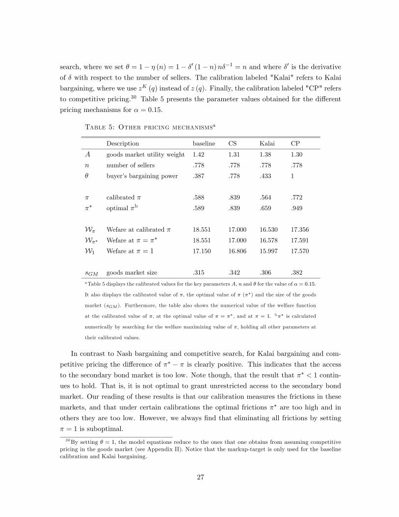
to competitive pricing.30 Table 5 presents the parameter values obtained for the di¤erent

pricing mechanisms for � = 0:15.

Table 5: Other pricing mechanismsa

Description baseline CS Kalai CP

A goods market utility weight 1.42 1.31 1.38 1.30

n number of sellers .778 .778 .778 .778

� buyer�s bargaining power .387 .778 .433 1

� calibrated � .588 .839 .564 .772

�� optimal �b .589 .839 .659 .949

W� Wefare at calibrated � 18.551 17.000 16.530 17.356

W�� Wefare at � = �� 18.551 17.000 16.578 17.591

W1 Wefare at � = 1 17.150 16.806 15.997 17.570

sGM goods market size .315 .342 .306 .382aTable 5 displays the calibrated values for the key parameters A, n and � for the value of � = 0:15.

It also displays the calibrated value of �, the optimal value of � (��) and the size of the goods

market (sGM ). Furthermore, the table also shows the numerical value of the welfare function

at the calibrated value of �, at the optimal value of � = ��, and at � = 1. b�� is calculated

numerically by searching for the welfare maximizing value of �, holding all other parameters at

their calibrated values.

In contrast to Nash bargaining and competitive search, for Kalai bargaining and com-

petitive pricing the di¤erence of �� � � is clearly positive. This indicates that the accessto the secondary bond market is too low. Note though, that the result that �� < 1 contin-

ues to hold. That is, it is not optimal to grant unrestricted access to the secondary bond

market. Our reading of these results is that our calibration measures the frictions in these

markets, and that under certain calibrations the optimal frictions �� are too high and in

others they are too low. However, we always �nd that eliminating all frictions by setting

� = 1 is suboptimal.

30By setting � = 1; the model equations reduce to the ones that one obtains from assuming competitivepricing in the goods market (see Appendix II). Notice that the markup-target is only used for the baselinecalibration and Kalai bargaining.

27

Compared to Nash bargaining, the pricing mechanims competitive search and com-

petitive pricing result on average in a higher goods market share on total output. For

competitive search, we obtain at the lower end sGM = 34%, while at the upper end we

obtain sGM = 38% under competitive pricing.

8 Conclusion

We construct a general equilibrium model with a liquid asset (�at money) and an illiquid

asset (a one-period government bond). Agents experience idiosyncratic liquidity shocks

after which they can trade these assets in a secondary bond market. We �nd that an agent�s

portfolio choice of liquid and illiquid assets involves a pecuniary externality. An agent does

not take into account that by holding more of the liquid asset he not only acquires additional

insurance against his own idiosyncratic liquidity risks, but he also marginally increases the

value of the liquid asset which improves insurance for other market participants. This

pecuniary externality can be corrected by restricting, but not eliminating, access to the

secondary bond market.

The key result is that it can be optimal to reduce the frequency of trading in �nancial

markets. This result is consistent with current attempts by the European Parliament to

introduce a �nancial-transactions tax, in order to generate revenue and to dampen excessive

trading.

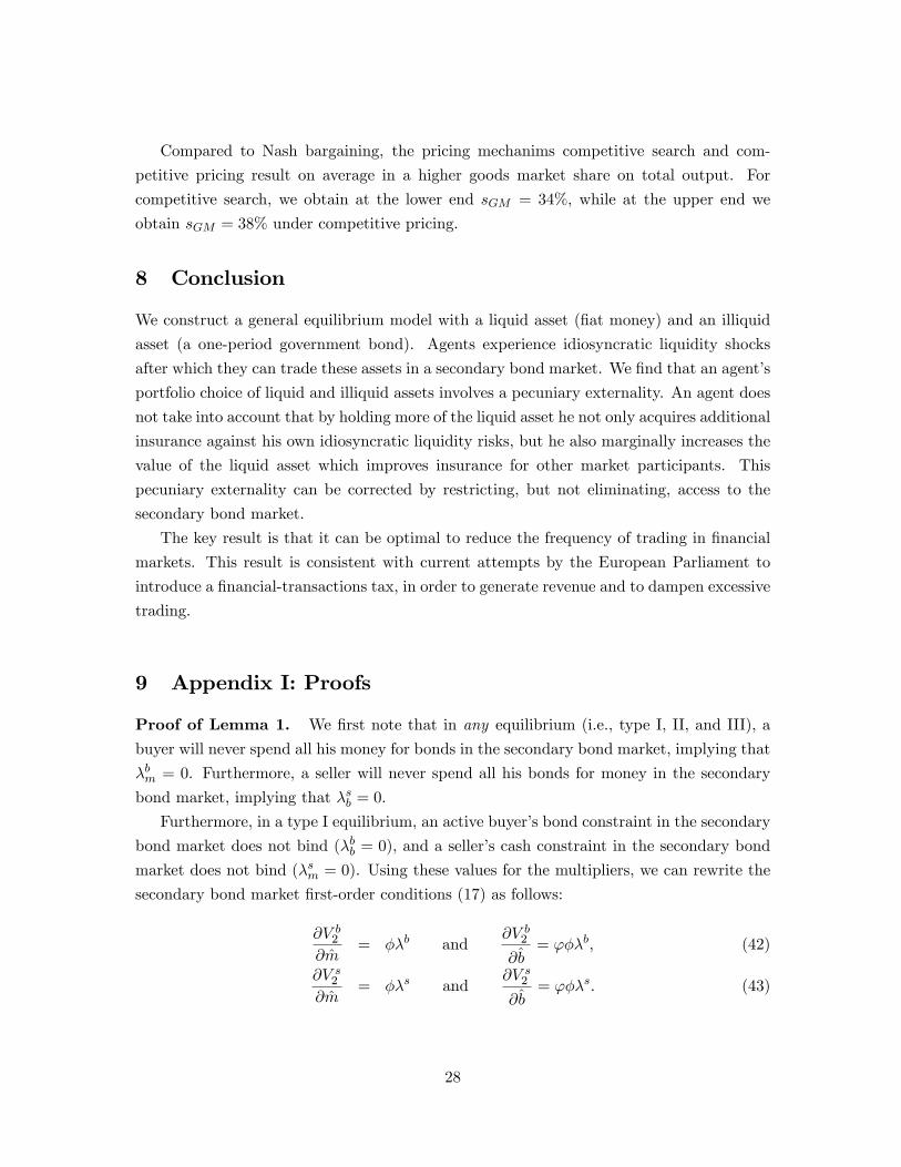
9 Appendix I: Proofs

Proof of Lemma 1. We �rst note that in any equilibrium (i.e., type I, II, and III), a

buyer will never spend all his money for bonds in the secondary bond market, implying that

�bm = 0. Furthermore, a seller will never spend all his bonds for money in the secondary

bond market, implying that �sb = 0.

Furthermore, in a type I equilibrium, an active buyer�s bond constraint in the secondary

bond market does not bind (�bb = 0), and a seller�s cash constraint in the secondary bond

market does not bind (�sm = 0). Using these values for the multipliers, we can rewrite the

secondary bond market �rst-order conditions (17) as follows:

@V b2@m̂

= ��b and@V b2

@b̂= '��b, (42)

@V s2@m̂

= ��s and@V s2

@b̂= '��s. (43)

28

Furthermore, combining the previous expressions with (12) and (14), we have

�b = �u0(q̂)

z0 (q̂)+ 1� � and '�b = 1, (44)

�s = 1 and '�s = 1. (45)

Then, (45) implies that ' = 1; i.e., that (23) holds.

Then, from (44), the fact that ' = 1 immediately implies that �b = 1, which then

implies that u0(q̂) = z0 (q̂); i.e., that (26) holds.

Use (12) and (14) to write (18) and (19) as follows:

@V1@m

= ��h(1� n)�b + n�s

i+ (1� �) [(1� n)�(q) + n�] ; (46)

@V1@b

= ��h(1� n)'�b + n'�s

i+ (1� �) [(1� n)�+ n�] : (47)

Use the primary bond market �rst order conditions (5) to write the previous equations as

follows

�= �

h(1� n)�b + n�s

i+ (1� �) [(1� n) (q) + n] ; (48)

�

�= �'

h(1� n)�b + n�s

i+ 1� �: (49)

We have already established that in the type I equilibrium �b = �s = ' = 1. This implies,

from (49), that � = �= ; i.e., that equation (25) holds. Finally, (24) immediately follows

from (48).

Note that if � < 1, active buyers consume the ine¢ cient quantity, since q̂ < q� even as

� ! . If � = 1, u0(q̂) = 1; so they consume the e¢ cient quantity q̂ = q�.

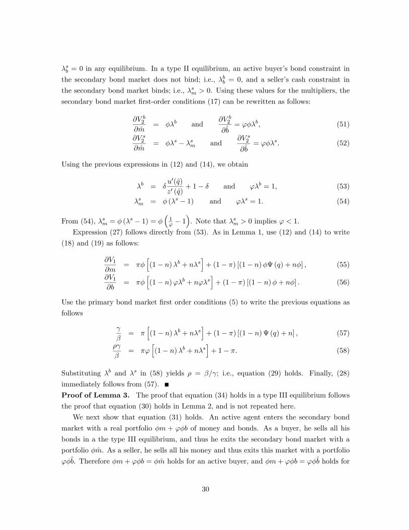
Proof of Lemma 2. We �rst show that equation (30) holds. In the type II equilibrium, all

buyers spend all their money in the goods market. Consequently, z(q) = m� and z(q̂) = m̂�

hold. The last two equations imply

z(q) = z(q̂)m=m̂: (50)

Each active buyer exits the secondary bond market with m̂ units of money, while an active

seller exits with zero units of money. A passive agent (a seller or a buyer) exits the secondary

bond market with m units of money, therefore M�1 = (1 � n)�m̂ + n� � 0 + (1� �)m.Replacing m = M�1, we get m̂ = M�1=(1 � n). Use m̂ = M�1=(1 � n) and m = M�1 to

replace m̂ and m in (50), respectively, to get z(q) = z(q̂)(1� n); i.e., equation (30) holds.We now show that (27)-(29) hold. As argued in the proof of Lemma 1, �bm = 0 and

29

�sb = 0 in any equilibrium. In a type II equilibrium, an active buyer�s bond constraint in

the secondary bond market does not bind; i.e., �bb = 0, and a seller�s cash constraint in

the secondary bond market binds; i.e., �sm > 0. Using these values for the multipliers, the

secondary bond market �rst-order conditions (17) can be rewritten as follows:

@V b2@m̂

= ��b and@V b2

@b̂= '��b, (51)

@V s2@m̂

= ��s � �sm and@V s2

@b̂= '��s. (52)

Using the previous expressions in (12) and (14), we obtain

�b = �u0(q̂)

z0 (q̂)+ 1� � and '�b = 1, (53)

�sm = � (�s � 1) and '�s = 1. (54)

From (54), �sm = � (�s � 1) = �

�1' � 1

�. Note that �sm > 0 implies ' < 1.

Expression (27) follows directly from (53). As in Lemma 1, use (12) and (14) to write

(18) and (19) as follows:

@V1@m

= ��h(1� n)�b + n�s

i+ (1� �) [(1� n)�(q) + n�] ; (55)

@V1@b

= ��h(1� n)'�b + n'�s

i+ (1� �) [(1� n)�+ n�] : (56)

Use the primary bond market �rst order conditions (5) to write the previous equations as

follows

�= �

h(1� n)�b + n�s

i+ (1� �) [(1� n) (q) + n] ; (57)

�

�= �'

h(1� n)�b + n�s

i+ 1� �: (58)

Substituting �b and �s in (58) yields � = �= ; i.e., equation (29) holds. Finally, (28)

immediately follows from (57).

Proof of Lemma 3. The proof that equation (34) holds in a type III equilibrium follows

the proof that equation (30) holds in Lemma 2, and is not repeated here.

We next show that equation (31) holds. An active agent enters the secondary bond

market with a real portfolio �m + '�b of money and bonds. As a buyer, he sells all his

bonds in a the type III equilibrium, and thus he exits the secondary bond market with a

portfolio �m̂. As a seller, he sells all his money and thus exits this market with a portfolio

'�b̂. Therefore �m+ '�b = �m̂ holds for an active buyer, and �m+ '�b = '�b̂ holds for

30

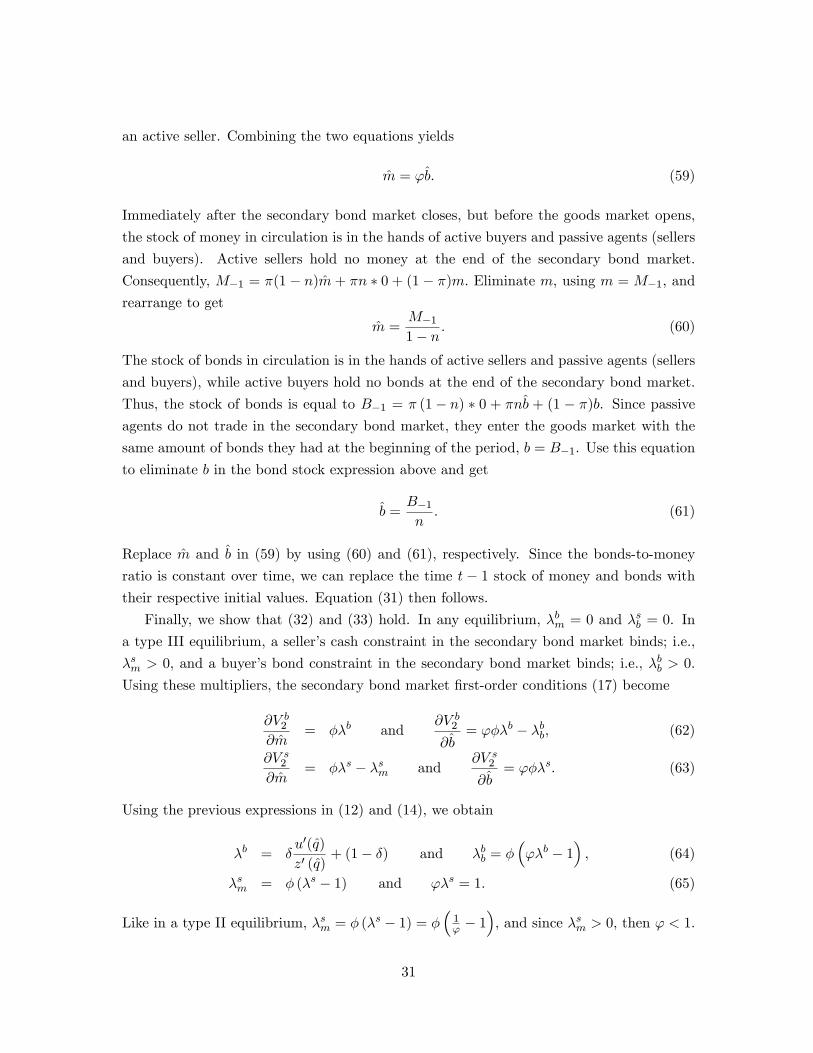
an active seller. Combining the two equations yields

m̂ = 'b̂: (59)

Immediately after the secondary bond market closes, but before the goods market opens,

the stock of money in circulation is in the hands of active buyers and passive agents (sellers

and buyers). Active sellers hold no money at the end of the secondary bond market.

Consequently, M�1 = �(1 � n)m̂ + �n � 0 + (1 � �)m: Eliminate m, using m = M�1, and

rearrange to get

m̂ =M�11� n: (60)

The stock of bonds in circulation is in the hands of active sellers and passive agents (sellers

and buyers), while active buyers hold no bonds at the end of the secondary bond market.

Thus, the stock of bonds is equal to B�1 = � (1� n) � 0 + �nb̂ + (1 � �)b. Since passiveagents do not trade in the secondary bond market, they enter the goods market with the

same amount of bonds they had at the beginning of the period, b = B�1. Use this equation

to eliminate b in the bond stock expression above and get

b̂ =B�1n: (61)

Replace m̂ and b̂ in (59) by using (60) and (61), respectively. Since the bonds-to-money

ratio is constant over time, we can replace the time t � 1 stock of money and bonds withtheir respective initial values. Equation (31) then follows.

Finally, we show that (32) and (33) hold. In any equilibrium, �bm = 0 and �sb = 0. In

a type III equilibrium, a seller�s cash constraint in the secondary bond market binds; i.e.,

�sm > 0, and a buyer�s bond constraint in the secondary bond market binds; i.e., �bb > 0.

Using these multipliers, the secondary bond market �rst-order conditions (17) become

@V b2@m̂

= ��b and@V b2

@b̂= '��b � �bb, (62)

@V s2@m̂

= ��s � �sm and@V s2

@b̂= '��s. (63)

Using the previous expressions in (12) and (14), we obtain

�b = �u0(q̂)

z0 (q̂)+ (1� �) and �bb = �

�'�b � 1

�, (64)

�sm = � (�s � 1) and '�s = 1. (65)

Like in a type II equilibrium, �sm = � (�s � 1) = �

�1' � 1

�, and since �sm > 0; then ' < 1.

31

Unlike in a type II equilibrium, from (62), we �nd �bb = ��'�b � 1

�= � ['(q̂)� 1]. Since

�bb > 0, (q̂) > 1='; and so (27) does not hold in a type III equilibrium.

Use (12) and (14) to write (18) and (19) as follows:

@V1@m

= ��h(1� n)�b + n�s

i+ (1� �) [(1� n)�(q) + n�] ; (66)

@V1@b

= ��h(1� n)'�b + n'�s

i+ (1� �) [(1� n)�+ n�] : (67)

Using the primary bond market �rst-order conditions (5), the previous equations can be

rewritten as follows:

�= �

h(1� n)�b + n�s

i+ (1� �) [(1� n) (q) + n] ; (68)

�

�= �'

h(1� n)�b + n�s

i+ 1� �: (69)

Substituting �b and �s in (68) and (69) yields (32) and (33), respectively.

Proof of Proposition 1. Derivation of L. The critical value L is the value of suchthat expressions (24) and (28) hold simultaneously; i.e., such that (q̂) = 1. Such a value

exists and is unique, since we assume that (q) is decreasing in q.

Derivation of H . The critical value H is the value of such that equations (28)

and (32) hold simultaneously; i.e., such that (q̂) = B0M0

1�nn > 1. Again, such a value exists

and is unique, since we assume that (q) is decreasing in q.

Proof of Lemma 4. From the buyer�s problem in the secondary bond market, V b1 (m; b) =

V b2 (m̂; b̂), where m̂ and b̂ are the quantities of money and bonds that maximize V b2 . In any

equilibrium, the buyer�s budget constraint (15) holds with equality. Thus, we can use (15)

to eliminate b̂ from V b2 (m̂; b̂) and get

V b1 (m; b) = Vb2

�m̂;�m+ '�b� �m̂

'�

�: (70)

Next, use (4), (10), and (3), to get

V b1 (m; b) = � fu [q (m̂)]� �d (m̂)g+ U(x�)� x� + �m̂+ �T � �m+1

+�m+ '�b� �m̂

'� ��b+1 + �V1(m+1; b+1): (71)

Note that the buyer�s cash constraint in the goods market binds; i.e., d (m̂) = m̂. From

(2), T = M �M�1 + �B � B�1, and the budget constraint in the goods market satis�esm̂� = z (q̂) and m� = z (q). Furthermore, all agents exit the period with the same amount

of money and bonds, hence m+1 =M and b+1 = B. Using these equalities we can rewrite

32

(71) as follows:

V b1 (m; b) = � [u (q̂)� z (q̂)] + U(x�)� x�

��1

'� 1�[z (q̂)� z (q)] + �V1(m+1; b+1);

where we have used b = B�1 and m =M�1: Another way to write this is

V b1 (m; b) = � [u (q̂)� z (q̂)] + U(x�)� x� � i [z (q̂)� z (q)] + �V1(m+1; b+1): (72)

The active buyer�s period surplus is � [u (q̂)� z (q̂)], but he has to pay interest i = 1' � 1

on the di¤erence z (q̂)� z (q) :Along the same lines, for a passive agent one can show that

V b2 (m; b) = � [u (q)� z (q)] + U(x�)� x� + �V1(m+1; b+1): (73)

The di¤erence between (72) and (73) is

V b1 (m; b)� V b2 (m; b) = � [u (q̂)� z (q̂)]� � [u (q)� z (q)]� i [z (q̂)� z (q)] : (74)

We now need to study (74) for the di¤erent types of equilibria. For the type I equilibrium,

' comes from (23), thus

V b1 (m; b)� V b2 (m; b) = 1 � � [u (q̂)� z (q̂)]� � [u (q)� z (q)] > 0;

which is clearly strictly positive, since q < q̂. For the type II equilibrium, ' comes from

(27), thus

2 � � [u (q̂)� z (q̂)]� � [u (q)� z (q)]� ��u0(q̂)

z0 (q̂)� 1�[z (q̂)� z (q)] : (75)

For the type III equilibrium, ' comes from (31), thus

3 � � [u (q̂)� z (q̂)]� � [u (q)� z (q)]��B0M0

1� nn

� 1�[z (q̂)� z (q)] :

Note that in the type III equilibrium we have � u0(q̂)z0(q̂) + 1 � � �

1' =

B0M0

1�nn . Accordingly,

3 � 2. Hence, it is su¢ cient to show that 2 > 0. To do so, rewrite (75) as follows:

u (q̂)� u (q)� z (q̂) + z (q) >�u0(q̂)

z0 (q̂)� 1�[z (q̂)� z (q)] :

33

Divide both sides of the above inequality by q̂ � q and rearrange it to get

u(q̂)�u(q)q̂�q

z(q̂)�z(q)q̂�q

>u0(q̂)

z0 (q̂).

The left-hand side is larger than the right-hand side, since we have assumed that u0(q)z0(q) is a

strictly decreasing function of q. Hence, 3 � 2 > 0.Proof of Lemma 5. From an active seller�s decision problem in the secondary bond

market, V s1 (m; b) = Vs2 (m̂; b̂). In any equilibrium, the seller�s budget constraint (15) holds

with equality. Thus, we can use (15) to eliminate b̂ from V s2 (m̂; b̂) and get

V s1 (m; b) = Vs2

��m̂;

�m+ '�b� �m̂'�

�: (76)

Using (13), the following holds

V s1 (m; b) = �s [�c (q) + �d] + V3

�m̂;�m+ '�b� �m̂

'�

�;

which can be rewritten as follows:

V s1 (m; b) = �s [�c (q) + �d] + U(x�)� x� + �m̂+ �m+ '�b� �m̂'

+�T � �m+1 � ��b+1 + �V1(m+1; b+1);

by virtue of (3) and (4).

For a passive seller, one can show that

V s2 (m; b) = �s [�c (q) + �d] + U(x�)� x� + �m+ �b

+�T � �m+1 � ��b+1 + �V1(m+1; b+1):

Hence the di¤erence V s1 (m; b)� V s2 (m; b) is equal to

V s1 (m; b)� V s2 (m; b) = �m̂� �m+�m� �m̂

'= i (�m� �m̂) :

Note that active sellers do not carry any money into the goods market, thus �m̂ = 0. Also

note that �m = z (q) > 0. It turns out that the above di¤erence is positive if i > 0.

34

10 Appendix II: Competitive Markets

Under competitive pricing, buyers and sellers take the price of goods as given in the goods

market. Under competitive pricing, it is natural to interpret � and �s as participation

probabilities in the goods market. In particular, let � (�s) be the probability that a buyer

(seller) participates in the goods market. Then the buyer�s value function in the goods

market is

V b2 (m; b) = �maxq

"u (q) + V3 (m� pq; b)

s.t. m � pq:

#+ (1� �)V3(m; b); (77)

where p is the price, and q the quantity of market-2 goods consumed by the buyer. The

�rst-order condition to this problem is

u0(q) = p (�+ �q) ; (78)

where �q is the Lagrange multiplier on m � pq.The seller�s value function in the goods market is

V s2 (m; b) = �smax

qs[�c (qs) + V3 (m+ pqs; b)] + (1� �s)V3(m; b): (79)

The �rst-order condition to this problem is

p� = c0 (qs) : (80)

If the buyer�s cash constraint is not binding, the buyer consumes the e¢ cient quantity q�,

where q� solves u0(q) = c0 (qs). If the cash constraint is binding, then he spends all his

money in goods purchases, and consumption is ine¢ ciently low. Note that, in equilibrium,

an active buyer will hold more money than a passive buyer. This means that �q > �̂q. It

then follows that q̂ > q.

The buyer�s envelope conditions are

@V b2@m

= ��u0 (q)

c0 (q)+ (1� �)� and

@V b2@b

= �; (81)

where we have used the envelope conditions in the primary bond market, and the �rst-

order conditions in the goods market. Notice the similarity between (81) and (12). The

two expressions are the same if � = 1. As a consequence of this, active buyers consume

the e¢ cient quantity in a type I equilibrium under competitive pricing, while they do not

under bilateral matching unless � = 1.

The seller�s envelope conditions are exactly the same as (14); i.e., @Vs2

@m =@V s2@b = �.

35

Finally, by using the budget constraint of the buyer at equality pq = m and (80) we get

�m = zC (q) � c0 (qs) q;

which is equal to (38) for a linear cost function.

11 Appendix III: Competitive Search

As an alternative trading mechanism we consider the competitive search framework pro-

posed by Moen (1997) and Mortensen and Wright (2002), and used in Rocheteau and

Wright (2005, 2009). Here, we follow the derivation of the competitive search equilibrium

presented in Rocheteau and Wright (2005). We refer to their paper for additional details.

There are agents called submarket makers, who set up submarkets in the goods market

and charge an entry fee to participants. This fee is zero in equilibrium, since submarkets

can be opened costlessly. Any given submarket is characterized by the terms of trade (q; d)

and the number of buyers and sellers (1� n; n). The timing of the events is as follows.At the beginning of each period, submarket makers announce the terms of trade for each

trading post. Given (q; d), agents decide where to go. In each submarket, the terms of

trade are predetermined, so agents do not bargain once in a match; however, they still have

to search for their partner and may end up without having a match.

Submarket makers design submarkets by maximizing the buyers�payo¤s subject to the

constraint that a positive number of sellers enter the markets. Note that active buyers and

passive buyers may want to consume di¤erent quantities, since the former can adjust their

balance after the production/consumption shock, while the latter cannot. It turns out that

market makers may �nd it pro�table to design di¤erent types of submarkets for di¤erent

types of buyers. In equilibrium, two types of submarkets are open: submarkets for active

buyers and submarkets for passive buyers. Nevertheless, in what follows, we can derive the

terms of trade in a submarket for agents with money holdings m.

The market maker problem for such a submarket is

maxn;q;d

� [u (q) + V3 (m� d; b)] + (1� �)V3 (m; b) s.t.

�s [�c (q) + �d] = J and d � m;

where J is the equilibrium expected utility of a seller in the goods market (for more details

see Rocheteau and Wright, 2005).

This submarket is designed for buyers with money holdings m. Once in this market,

they can consume with probability �, and they cannot with probability 1 � �. The �rst

36

constraint ensures that a positive number of sellers enter the submarket. Given q and d,

this constraint yields n. The second constraint follows from the fact that buyers cannot

spend more money than the amount they bring into the goods market.

We can use the linearity of the value function V3 to rewrite the market maker problem

as follows:

maxn;q;d

� [u (q)� �d] + V3 (m; b) s.t.

�s [�c (q) + �d] = J and d � m.

If the second constraint binds, i.e., d = m, the problem above reduces to

maxn;q

� [u (q)� �m] + V3 (m; b) s.t.

�s [�c (q) + �m] = J:

If we denote � the Lagrangian multiplier of the constraint, the �rst-order conditions are

�0 [u (q)� �m]� � [�c (q) + �m] �0 (1� n)n� �

n2= 0;

�u0 (q) + �c0 (q)� (1� n)

n= 0:

where �0 is the derivative of � with respect to the number of sellers. Substituting � from

the �rst into the second equations yields

�0 [u (q)� �m] + u0 (q) [�c (q) + �m](1� n) c0 (q)

�0 (1� n)n� �n

= 0:

Solving for �m yields �m = zP (q), where

zP (q) � [1� � (n)] c (q)u0(q) + � (n)u(q)c0 (q)[1� � (n)]u0(q) + � (n) c0 (q) ; (82)

which is the same as (36). Note that � (n) � �0(1�n)n� is the seller�s contribution to the

matching process; i.e., the elasticity of the matching function with respect to the measures of

sellers. Notice that (82) is the solution of the bargaining problem when � = 1�� (n). Hence,with competitive search, the Hosios condition is automatically satis�ed (for a discussion of

e¢ ciency in matching models see Hosios, 1990).

37

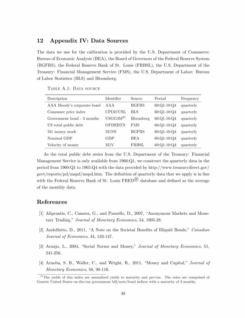
12 Appendix IV: Data Sources

The data we use for the calibration is provided by the U.S. Department of Commerce:

Bureau of Economic Analysis (BEA), the Board of Governors of the Federal Reserve System

(BGFRS), the Federal Reserve Bank of St. Louis (FRBSL), the U.S. Department of the

Treasury: Financial Management Service (FMS), the U.S. Department of Labor: Bureau

of Labor Statistics (BLS) and Bloomberg.

Table A.1: Data source

Description Identi�er Source Period Frequency

AAA Moody�s corporate bond AAA BGFRS 60:Q1-10:Q4 quarterly

Consumer price index CPIAUCSL BLS 60:Q1-10:Q4 quarterly

Government bond - 3 months USGG3M31 Bloomberg 60:Q1-10:Q4 quarterly

US total public debt GFDEBTN FMS 66:Q1-10:Q4 quarterly

M1 money stock M1NS BGFRS 60:Q1-10:Q4 quarterly

Nominal GDP GDP BEA 60:Q1-10:Q4 quarterly

Velocity of money M1V FRBSL 60:Q1-10:Q4 quarterly

As the total public debt series from the U.S. Department of the Treasury: Financial

Management Service is only available from 1966:Q1, we construct the quarterly data in the

period from 1960:Q1 to 1965:Q4 with the data provided by http://www.treasurydirect.gov/

govt/reports/pd/mspd/mspd.htm. The de�nition of quarterly data that we apply is in line

with the Federal Reserve Bank of St. Louis FRED R database and de�ned as the average

of the monthly data.

References

[1] Aliprantis, C., Camera, G., and Puzzello, D., 2007, �Anonymous Markets and Mone-

tary Trading,�Journal of Monetary Economics, 54, 1905-28.

[2] Andolfatto, D., 2011, �A Note on the Societal Bene�ts of Illiquid Bonds,�Canadian

Journal of Economics, 44, 133-147.

[3] Araujo, L., 2004, �Social Norms and Money,� Journal of Monetary Economics, 51,

241-256.

[4] Aruoba, S. B., Waller, C., and Wright, R., 2011, �Money and Capital,� Journal of

Monetary Economics, 58, 98-116.31The yields of this index are annualized yields to maturity and pre-tax. The rates are comprised of

Generic United States on-the-run government bill/note/bond indices with a maturity of 3 months.

38

[5] Aruoba, B., Rocheteau, G., and Waller, C., 2007, �Bargaining and the Value of

Money,�Journal of Monetary Economics, 54, 2636-2655.

[6] Berentsen, A., Camera, G., and Waller, C., 2007, �Money, Credit and Banking,�Jour-

nal of Economic Theory, 135, 171-195.

[7] Berentsen, A., and Waller, C., 2011, �Outside Versus Inside Bonds: A Modigliani-

Miller Type Result for Liquidity Constrained Economies,�Journal of Economic The-

ory, 146, 1852-1887.

[8] Berentsen, A., Menzio, G., and Wright, R., 2011, �In�ation and Unemployment in the

Long Run,�American Economic Review, 101, 371-98.

[9] Bernanke, B., and Gertler, M., 1989, �Agency Costs, Net Worth, and Business Fluc-

tuations,�American Economic Review, 79, 14-31.

[10] Bianchi, J., 2011, �Overborrowing and Systemic Externalities in the Business Cycle,�

American Economic Review, 101, 3400-3426.

[11] Bianchi, J., and Mendoza, E. G., 2011, �Overborrowing, Financial Crises and �Macro-

prudential�Policy,�International Monetary Found, working paper # 11/24.

[12] Boel, P., and Camera, G., 2006 �E¢ cient Monetary Allocations and the Illiquidity of

Bonds,�Journal of Monetary Economics, 53, 1693-715.

[13] Caballero, R. J., and Krishnamurthy, A., 2003, �Excessive Dollar Debt: Financial

Development and Underinsurance,�Journal of Finance, 58, 867-894.

[14] Faig, M., and Jerez, B., 2005, �A Theory of Commerce,�Journal of Economic Theory,

122, 60-99.

[15] Geromichalos, A., and Herrenbrueck, L., 2012, �Monetary Policy, Asset Prices, and

Liquidity in Over-the-Counter Markets,�UC Davis, working paper # 12-20.

[16] Geromichalos, A., Licari, J. M., and Lledo, J. S., 2007, �Monetary Policy and Asset

Prices,�Review of Economic Dynamics, 10, 761-779.

[17] He, C., Wright, R., and Zhu, Y., 2012, �Housing and Liquidity,�working paper, Uni-

versity of Wisconsin-Madison.

[18] Hosios, A., 1990, �On the E¢ cieny of Matching and Related Models of Search and

Unemployment,�Review of Economic Studies, 57, 279-298.

39

[19] Jeanne, O., and Korinek, A., 2012, �Managing Credit Booms and Busts: A Pigouvian

Taxation Approach�, working paper, University of Maryland.

[20] Kalai, E., 1977, �Proportional Solutions to Bargaining Situations: Interpersonal Utility

Comparisons,�Econometrica, 45, 1623-1630.

[21] Kehoe, T., and Levine, D., 1993, �Debt-constrained Asset Markets,�Review of Eco-

nomic Studies, 60, 865-888.

[22] Kiyotaki, N., and Moore, J., 1997, �Credit Cycles,�Journal of Political Economy, 105,

211-248.

[23] Kiyotaki, N., and Wright, R., 1993 �A Search-theoretic Approach to Monetary Eco-

nomics,�American Economic Review, 83, 63-77.

[24] Kocherlakota, N., 1998, �Money is Memory,�Journal of Economic Theory, 81, 232-251.

[25] Kocherlakota, N., 2003, �Social Bene�ts of Illiquid Bonds,�Journal of Economic The-

ory, 108, 179-193.

[26] Korinek, A., 2012, �Systemic Risk-Taking: Ampli�cation E¤ects, Externalities, and

Regulatory Responses,�working paper, University of Maryland.

[27] Lagos, R., and Rocheteau, G., 2007, �Search in Asset Markets: Market Structure,

Liquidity, and Welfare,�American Economic Review, 97, 198-202.

[28] Lagos, R., and Rocheteau, G., 2008, �Money and Capital as Competing Media of

Exchange,�Journal of Economic Theory, 142, 247-258.

[29] Lagos, R., and Rocheteau, G., 2009, �Liquidity in Asset Markets With Search Fric-

tions,�Econometrica, 77, 403-426.

[30] Lagos, R., and Wright, R., 2005, �A Uni�ed Framework for Monetary Theory and

Policy Evaluation,�Journal of Political Economy, 113, 463-484.

[31] Lester, B., Postelwaite, A., and Wright, R., 2012, �Information, Liquidity, Asset Prices

and Monetary Policy,�Review of Economic Studies, 79, 1209-1238.

[32] Lorenzoni, G., 2008. "Ine¢ cient Credit Booms," Review of Economic Studies, 75, 809-

833.

[33] Martin, F., 2012, �Debt, In�ation and Central Bank Independence,�working paper,

FRB of St. Louis.

40

[34] Mendoza, E. G., 2010, �Sudden Stops, Financial Crises, and Leverage,� American

Economic Review, 100, 1941-1966.

[35] Mendoza, E. G., and Smith, K., 2006, �Quantitative Implications of a Debt-de�ation

Theory of Sudden Stops and Asset Prices,� Journal of International Economics, 70,

82-114.

[36] Moen, E. R., 1997, �Competitive Search Equilibrium,�Journal of Political Economy,

105, 385-411.

[37] Mortensen, D., and Wright, R., 2002, �Competitive Pricing and E¢ ciency in Search

Equilibrium,�International Economic Review, 43, 1-20.

[38] Nosal, E., and Rocheteau, G., 2011, �Money, Payments, and Liquidity,� The MIT

Press.

[39] Rocheteau, G., and Weill, P. O., 2011, �Liquidity in Frictional Asset Markets,�Journal

of Money, Credit and Banking, 43, 261-282.

[40] Rocheteau, G., and Wright, R., 2005, �Money in Competitive Equilibrium, in Search

Equilibrium, and in Competitive Search Equilibrium,�Econometrica, 73, 175-202.

[41] Rocheteau, G., and Wright, R., 2009, �In�ation and Welfare in Models with Trading

Frictions,� in Monetary Policy in Low In�ation Economies, by Ed Nosal and Dave

Altig, Cambridge University Press.

[42] Rocheteau, G., and Wright, R., 2010, �Liquidity and Asset Market Dynamics,�working

paper, University of California, Irvine.

[43] Rojas-Breu, M., 2013, �The Welfare E¤ect of Access to Credit,�Economic Inquiry,

51, 235-247.

[44] Shi, S., 2008, �E¢ ciency Improvement from Restricting the Liquidity of Nominal

Bonds,�Journal of Monetary Economics, 55, 1025-1037.

[45] Trejos, A., andWright, R., 2012, �Shi-Trejos-Wright Meets Du¢ e-Garleanu-Pedersen,�

working paper, University of Wisconsin-Madison.

[46] Wallace, N., 2001, �Whither Monetary Economics?� International Economic Review,

42, 847-869.

[47] Wright, R., 2010, �A Uniqueness Proof for Monetary Steady State,�Journal of Eco-

nomic Theory, 145, 382-391.

41