Deformable Convolutional Networks - CVF Open Accessopenaccess.thecvf.com/.../Dai_Deformable_Convolutional_Networks... · Deformable Convolutional Networks Jifeng Dai∗ Haozhi Qi∗,†

Deformable Convolutional Networks

Jifeng Dai∗ Haozhi Qi∗,† Yuwen Xiong∗,† Yi Li∗,† Guodong Zhang∗,† Han Hu Yichen Wei

Microsoft Research Asia

{jifdai,v-haoq,v-yuxio,v-yii,v-guodzh,hanhu,yichenw}@microsoft.com

Abstract

Convolutional neural networks (CNNs) are inherently

limited to model geometric transformations due to the

fixed geometric structures in their building modules. In

this work, we introduce two new modules to enhance the

transformation modeling capability of CNNs, namely, de-

formable convolution and deformable RoI pooling. Both

are based on the idea of augmenting the spatial sampling

locations in the modules with additional offsets and learn-

ing the offsets from the target tasks, without additional

supervision. The new modules can readily replace their

plain counterparts in existing CNNs and can be easily

trained end-to-end by standard back-propagation, giving

rise to deformable convolutional networks. Extensive ex-

periments validate the performance of our approach. For

the first time, we show that learning dense spatial trans-

formation in deep CNNs is effective for sophisticated vi-

sion tasks such as object detection and semantic segmen-

tation. The code is released at https://github.com/

msracver/Deformable-ConvNets.

1. Introduction

A key challenge in visual recognition is how to accom-

modate geometric variations or model geometric transfor-

mations in object scale, pose, viewpoint, and part deforma-

tion. In general, there are two ways. The first is to build the

training datasets with sufficient desired variations. This is

usually realized by augmenting the existing data samples,

e.g., by affine transformation. Robust representations can

be learned from the data, but usually at the cost of expen-

sive training and complex model parameters. The second

is to use transformation-invariant features and algorithms.

This category subsumes many well known techniques, such

as SIFT (scale invariant feature transform) [38] and sliding

window based object detection paradigm.

There are two drawbacks in above ways. First, the geo-

∗Equal contribution. †This work is done when Haozhi Qi, Yuwen

Xiong, Yi Li and Guodong Zhang are interns at Microsoft Research Asia

metric transformations are assumed fixed and known. Such

prior knowledge is used to augment the data, and design the

features and algorithms. This assumption prevents general-

ization to new tasks possessing unknown geometric trans-

formations, which are not properly modeled. Second, hand-

crafted design of invariant features and algorithms could be

difficult or infeasible for overly complex transformations,

even when they are known.

Recently, convolutional neural networks (CNNs) [31]

have achieved significant success for visual recognition

tasks, such as image classification [27], semantic segmenta-

tion [37], and object detection [14]. Nevertheless, they still

share the above two drawbacks. Their capability of model-

ing geometric transformations mostly comes from the ex-

tensive data augmentation, the large model capacity, and

some simple hand-crafted modules (e.g., max-pooling [1]

for small translation-invariance).

In short, CNNs are inherently limited to model large,

unknown transformations. The limitation originates from

the fixed geometric structures of CNN modules: a con-

volution unit samples the input feature map at fixed loca-

tions; a pooling layer reduces the spatial resolution at a

fixed ratio; a RoI (region-of-interest) pooling layer sepa-

rates a RoI into fixed spatial bins, etc. There lacks internal

mechanisms to handle the geometric transformations. This

causes noticeable problems. For one example, the recep-

tive field sizes of all activation units in the same CNN layer

are the same. This is undesirable for high level CNN lay-

ers that encode the semantics over spatial locations. Be-

cause different locations may correspond to objects with

different scales or deformation, adaptive determination of

scales or receptive field sizes is desirable for visual recogni-

tion with fine localization, e.g., semantic segmentation us-

ing fully convolutional networks [37]. For another exam-

ple, while object detection has seen significant and rapid

progress [14, 47, 13, 42, 41, 36, 6] recently, all approaches

still rely on the primitive bounding box based feature extrac-

tion. This is sub-optimal, especially for non-rigid objects.

In this work, we introduce two new modules that greatly

enhance CNNs’ capability of modeling geometric transfor-

mations. The first is deformable convolution. It adds 2D

1764

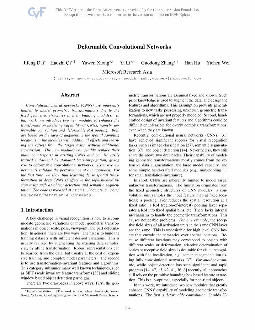
(a) (b) (c) (d)

Figure 1: Illustration of the sampling locations in 3 × 3standard and deformable convolutions. (a) regular sam-

pling grid (green points) of standard convolution. (b) de-

formed sampling locations (dark blue points) with aug-

mented offsets (light blue arrows) in deformable convolu-

tion. (c)(d) are special cases of (b), showing that the de-

formable convolution generalizes various transformations

for scale, (anisotropic) aspect ratio and rotation.

offsets to the regular grid sampling locations in the stan-

dard convolution. It enables free form deformation of the

sampling grid. It is illustrated in Figure 1. The offsets

are learned from the preceding feature maps, via additional

convolutional layers. Thus, the deformation is conditioned

on the input features in a local, dense, and adaptive manner.

The second is deformable RoI pooling. It adds an offset

to each bin position in the regular bin partition of the previ-

ous RoI pooling [13, 6]. Similarly, the offsets are learned

from the preceding feature maps and the RoIs, enabling

adaptive part localization for objects with different shapes.

Both modules are light weight. They add small amount

of parameters and computation for the offset learning. They

can readily replace their plain counterparts in deep CNNs

and can be easily trained end-to-end with standard back-

propagation. The resulting CNNs are called deformable

convolutional networks, or deformable ConvNets.

Our approach shares similar high level spirit with spatial

transform networks [23] and deformable part models [10].

They all have internal transformation parameters and learn

such parameters purely from data. A key difference in

deformable ConvNets is that they deal with dense spatial

transformations in a simple, efficient, deep and end-to-end

manner. In Section 3.1, we discuss in details the relation of

our work to previous works and analyze the superiority of

deformable ConvNets.

2. Deformable Convolutional Networks

The feature maps and convolution are 3D. Both de-

formable convolution and RoI pooling modules operate on

the 2D spatial domain. The operation remains the same

across the channel dimension. For simplicity, the modules

are described in 2D. Extension to 3D is straightforward.

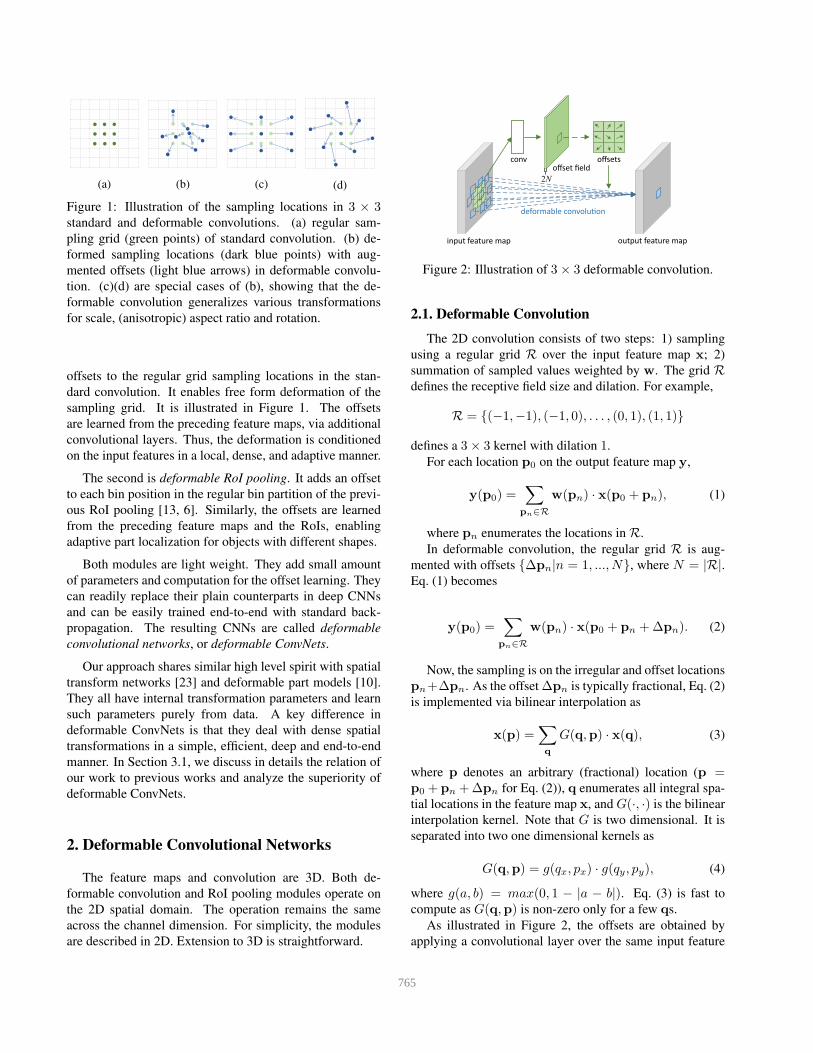
convoffset field

input feature map

2N

output feature map

deformable convolu�on

offsets

Figure 2: Illustration of 3× 3 deformable convolution.

2.1. Deformable Convolution

The 2D convolution consists of two steps: 1) sampling

using a regular grid R over the input feature map x; 2)

summation of sampled values weighted by w. The grid Rdefines the receptive field size and dilation. For example,

R = {(−1,−1), (−1, 0), . . . , (0, 1), (1, 1)}

defines a 3× 3 kernel with dilation 1.

For each location p0 on the output feature map y,

y(p0) =∑

pn∈R

w(pn) · x(p0 + pn), (1)

where pn enumerates the locations in R.

In deformable convolution, the regular grid R is aug-

mented with offsets {∆pn|n = 1, ..., N}, where N = |R|.Eq. (1) becomes

y(p0) =∑

pn∈R

w(pn) · x(p0 + pn +∆pn). (2)

Now, the sampling is on the irregular and offset locations

pn+∆pn. As the offset ∆pn is typically fractional, Eq. (2)

is implemented via bilinear interpolation as

x(p) =∑

q

G(q,p) · x(q), (3)

where p denotes an arbitrary (fractional) location (p =p0 + pn +∆pn for Eq. (2)), q enumerates all integral spa-

tial locations in the feature map x, and G(·, ·) is the bilinear

interpolation kernel. Note that G is two dimensional. It is

separated into two one dimensional kernels as

G(q,p) = g(qx, px) · g(qy, py), (4)

where g(a, b) = max(0, 1 − |a − b|). Eq. (3) is fast to

compute as G(q,p) is non-zero only for a few qs.

As illustrated in Figure 2, the offsets are obtained by

applying a convolutional layer over the same input feature

765

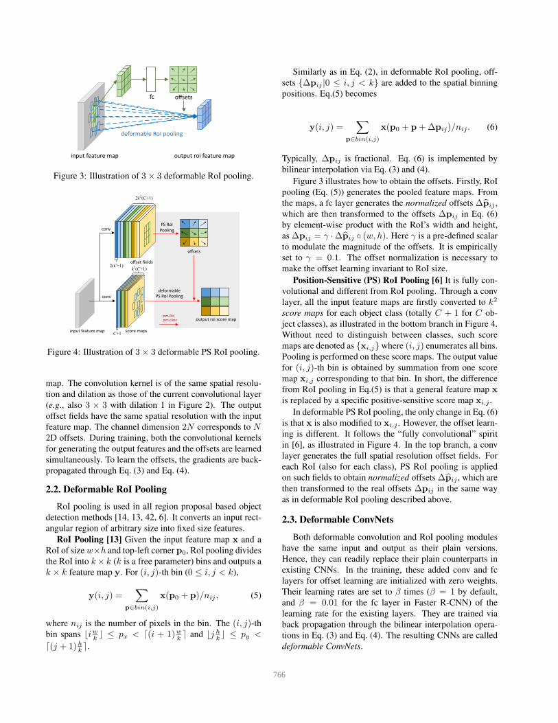
fc offsets

input feature map output roi feature map

deformable RoI pooling

Figure 3: Illustration of 3× 3 deformable RoI pooling.

PS RoI

Pooling

deformable

C+1

conv

conv

offset fields

score mapsinput feature map

per-RoIper-class

PS RoI Pooling

2k2(C+1)

2(C+1)k2(C+1)

output roi score map

offsets

Figure 4: Illustration of 3× 3 deformable PS RoI pooling.

map. The convolution kernel is of the same spatial resolu-

tion and dilation as those of the current convolutional layer

(e.g., also 3 × 3 with dilation 1 in Figure 2). The output

offset fields have the same spatial resolution with the input

feature map. The channel dimension 2N corresponds to N2D offsets. During training, both the convolutional kernels

for generating the output features and the offsets are learned

simultaneously. To learn the offsets, the gradients are back-

propagated through Eq. (3) and Eq. (4).

2.2. Deformable RoI Pooling

RoI pooling is used in all region proposal based object

detection methods [14, 13, 42, 6]. It converts an input rect-

angular region of arbitrary size into fixed size features.

RoI Pooling [13] Given the input feature map x and a

RoI of size w×h and top-left corner p0, RoI pooling divides

the RoI into k× k (k is a free parameter) bins and outputs a

k × k feature map y. For (i, j)-th bin (0 ≤ i, j < k),

y(i, j) =∑

p∈bin(i,j)

x(p0 + p)/nij , (5)

where nij is the number of pixels in the bin. The (i, j)-thbin spans ⌊iw

k⌋ ≤ px < ⌈(i + 1)w

k⌉ and ⌊j h

k⌋ ≤ py <

⌈(j + 1)hk⌉.

Similarly as in Eq. (2), in deformable RoI pooling, off-

sets {∆pij |0 ≤ i, j < k} are added to the spatial binning

positions. Eq.(5) becomes

y(i, j) =∑

p∈bin(i,j)

x(p0 + p+∆pij)/nij . (6)

Typically, ∆pij is fractional. Eq. (6) is implemented by

bilinear interpolation via Eq. (3) and (4).

Figure 3 illustrates how to obtain the offsets. Firstly, RoI

pooling (Eq. (5)) generates the pooled feature maps. From

the maps, a fc layer generates the normalized offsets ∆pij ,

which are then transformed to the offsets ∆pij in Eq. (6)

by element-wise product with the RoI’s width and height,

as ∆pij = γ ·∆pij ◦ (w, h). Here γ is a pre-defined scalar

to modulate the magnitude of the offsets. It is empirically

set to γ = 0.1. The offset normalization is necessary to

make the offset learning invariant to RoI size.

Position-Sensitive (PS) RoI Pooling [6] It is fully con-

volutional and different from RoI pooling. Through a conv

layer, all the input feature maps are firstly converted to k2

score maps for each object class (totally C + 1 for C ob-

ject classes), as illustrated in the bottom branch in Figure 4.

Without need to distinguish between classes, such score

maps are denoted as {xi,j} where (i, j) enumerates all bins.

Pooling is performed on these score maps. The output value

for (i, j)-th bin is obtained by summation from one score

map xi,j corresponding to that bin. In short, the difference

from RoI pooling in Eq.(5) is that a general feature map x

is replaced by a specific positive-sensitive score map xi,j .

In deformable PS RoI pooling, the only change in Eq. (6)

is that x is also modified to xi,j . However, the offset learn-

ing is different. It follows the “fully convolutional” spirit

in [6], as illustrated in Figure 4. In the top branch, a conv

layer generates the full spatial resolution offset fields. For

each RoI (also for each class), PS RoI pooling is applied

on such fields to obtain normalized offsets ∆pij , which are

then transformed to the real offsets ∆pij in the same way

as in deformable RoI pooling described above.

2.3. Deformable ConvNets

Both deformable convolution and RoI pooling modules

have the same input and output as their plain versions.

Hence, they can readily replace their plain counterparts in

existing CNNs. In the training, these added conv and fc

layers for offset learning are initialized with zero weights.

Their learning rates are set to β times (β = 1 by default,

and β = 0.01 for the fc layer in Faster R-CNN) of the

learning rate for the existing layers. They are trained via

back propagation through the bilinear interpolation opera-

tions in Eq. (3) and Eq. (4). The resulting CNNs are called

deformable ConvNets.

766

To integrate deformable ConvNets with the state-of-the-

art CNN architectures, we note that these architectures con-

sist of two stages. First, a deep fully convolutional network

generates feature maps over the whole input image. Sec-

ond, a shallow task specific network generates results from

the feature maps. We elaborate the two steps below.

Deformable Convolution for Feature Extraction We

adopt two state-of-the-art architectures for feature extrac-

tion: ResNet-101 [20] and a modifed version of Inception-

ResNet [46]. Both are pre-trained on ImageNet [7] dataset.

The original Inception-ResNet is designed for image

recognition. It has a feature misalignment issue and is prob-

lematic for dense prediction tasks. It is modified to fix the

alignment problem [18]. The modified version is dubbed as

“Aligned-Inception-ResNet”. Please find its details in the

online arxiv version of this paper.

Both models consist of several convolutional blocks, an

average pooling and a 1000-way fc layer for ImageNet clas-

sification. The average pooling and the fc layers are re-

moved. A randomly initialized 1 × 1 convolution is added

at last to reduce the channel dimension to 1024. As in com-

mon practice [3, 6], the effective stride in the last convo-

lutional block is reduced from 32 pixels to 16 pixels to in-

crease the feature map resolution. Specifically, at the begin-

ning of the last block, stride is changed from 2 to 1 (“conv5”

for both ResNet-101 and Aligned-Inception-ResNet). To

compensate, the dilation of all the convolution filters in this

block (with kernel size > 1) is changed from 1 to 2.

Optionally, deformable convolution is applied to the last

few convolutional layers (with kernel size > 1). We exper-

imented with different numbers of such layers and found 3as a good trade-off for different tasks, as reported in Table 1.

Segmentation and Detection Networks A task specific

network is built upon the output feature maps from the fea-

ture extraction network mentioned above.

In the below, C denotes the number of object classes.

DeepLab [4] is a state-of-the-art method for semantic

segmentation. It adds a 1 × 1 convolutional layer over the

feature maps to generates (C + 1) maps that represent the

per-pixel classification scores. A following softmax layer

then outputs the per-pixel probabilities.

Category-Aware RPN is almost the same as the region

proposal network in [42], except that the 2-class (object or

not) convolutional classifier is replaced by a (C + 1)-class

convolutional classifier.

Faster R-CNN [42] is the state-of-the-art detector. In our

implementation, the RPN branch is added on the top of the

conv4 block, following [42]. In the previous practice [20,

22], the RoI pooling layer is inserted between the conv4

and the conv5 blocks in ResNet-101, leaving 10 layers for

each RoI. This design achieves good accuracy but has high

per-RoI computation. Instead, we adopt a simplified design

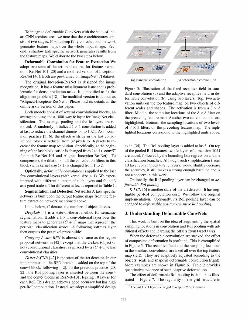
(a) standard convolution (b) deformable convolution

Figure 5: Illustration of the fixed receptive field in stan-

dard convolution (a) and the adaptive receptive field in de-

formable convolution (b), using two layers. Top: two acti-

vation units on the top feature map, on two objects of dif-

ferent scales and shapes. The activation is from a 3 × 3filter. Middle: the sampling locations of the 3 × 3 filter on

the preceding feature map. Another two activation units are

highlighted. Bottom: the sampling locations of two levels

of 3 × 3 filters on the preceding feature map. The high-

lighted locations correspond to the highlighted units above.

as in [34]. The RoI pooling layer is added at last1. On top

of the pooled RoI features, two fc layers of dimension 1024are added, followed by the bounding box regression and the

classification branches. Although such simplification (from

10 layer conv5 block to 2 fc layers) would slightly decrease

the accuracy, it still makes a strong enough baseline and is

not a concern in this work.

Optionally, the RoI pooling layer can be changed to de-

formable RoI pooling.

R-FCN [6] is another state-of-the-art detector. It has neg-

ligible per-RoI computation cost. We follow the original

implementation. Optionally, its RoI pooling layer can be

changed to deformable position-sensitive RoI pooling.

3. Understanding Deformable ConvNets

This work is built on the idea of augmenting the spatial

sampling locations in convolution and RoI pooling with ad-

ditional offsets and learning the offsets from target tasks.

When the deformable convolution are stacked, the effect

of composited deformation is profound. This is exemplified

in Figure 5. The receptive field and the sampling locations

in the standard convolution are fixed all over the top feature

map (left). They are adaptively adjusted according to the

objects’ scale and shape in deformable convolution (right).

More examples are shown in Figure 6. Table 2 provides

quantitative evidence of such adaptive deformation.

The effect of deformable RoI pooling is similar, as illus-

trated in Figure 7. The regularity of the grid structure in

1The last 1× 1 layer is changed to outputs 256-D features.

767

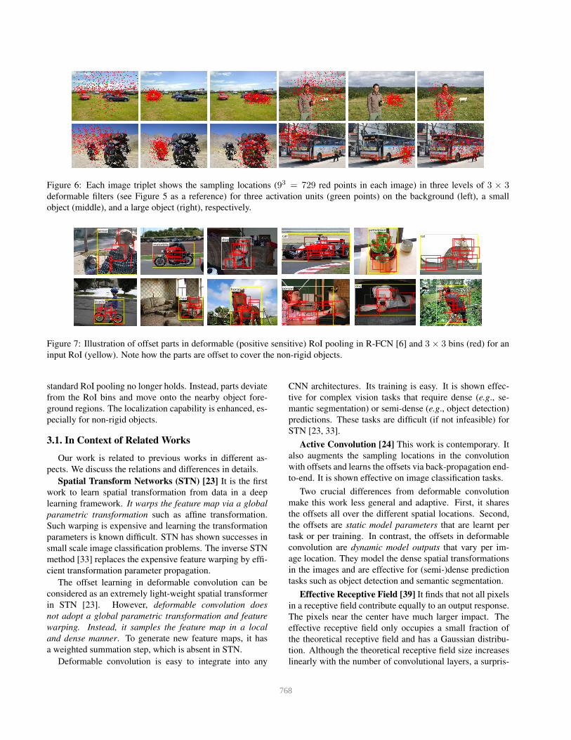
Figure 6: Each image triplet shows the sampling locations (93 = 729 red points in each image) in three levels of 3 × 3deformable filters (see Figure 5 as a reference) for three activation units (green points) on the background (left), a small

object (middle), and a large object (right), respectively.

cat

chair

car

pottedplant

person

motorbike

person

bicycle

horse

dog

dog bird

Figure 7: Illustration of offset parts in deformable (positive sensitive) RoI pooling in R-FCN [6] and 3 × 3 bins (red) for an

input RoI (yellow). Note how the parts are offset to cover the non-rigid objects.

standard RoI pooling no longer holds. Instead, parts deviate

from the RoI bins and move onto the nearby object fore-

ground regions. The localization capability is enhanced, es-

pecially for non-rigid objects.

3.1. In Context of Related Works

Our work is related to previous works in different as-

pects. We discuss the relations and differences in details.

Spatial Transform Networks (STN) [23] It is the first

work to learn spatial transformation from data in a deep

learning framework. It warps the feature map via a global

parametric transformation such as affine transformation.

Such warping is expensive and learning the transformation

parameters is known difficult. STN has shown successes in

small scale image classification problems. The inverse STN

method [33] replaces the expensive feature warping by effi-

cient transformation parameter propagation.

The offset learning in deformable convolution can be

considered as an extremely light-weight spatial transformer

in STN [23]. However, deformable convolution does

not adopt a global parametric transformation and feature

warping. Instead, it samples the feature map in a local

and dense manner. To generate new feature maps, it has

a weighted summation step, which is absent in STN.

Deformable convolution is easy to integrate into any

CNN architectures. Its training is easy. It is shown effec-

tive for complex vision tasks that require dense (e.g., se-

mantic segmentation) or semi-dense (e.g., object detection)

predictions. These tasks are difficult (if not infeasible) for

STN [23, 33].

Active Convolution [24] This work is contemporary. It

also augments the sampling locations in the convolution

with offsets and learns the offsets via back-propagation end-

to-end. It is shown effective on image classification tasks.

Two crucial differences from deformable convolution

make this work less general and adaptive. First, it shares

the offsets all over the different spatial locations. Second,

the offsets are static model parameters that are learnt per

task or per training. In contrast, the offsets in deformable

convolution are dynamic model outputs that vary per im-

age location. They model the dense spatial transformations

in the images and are effective for (semi-)dense prediction

tasks such as object detection and semantic segmentation.

Effective Receptive Field [39] It finds that not all pixels

in a receptive field contribute equally to an output response.

The pixels near the center have much larger impact. The

effective receptive field only occupies a small fraction of

the theoretical receptive field and has a Gaussian distribu-

tion. Although the theoretical receptive field size increases

linearly with the number of convolutional layers, a surpris-

768

ing result is that, the effective receptive field size increases

linearly with the square root of the number, therefore, at a

much slower rate than what we would expect.

This finding indicates that even the top layer’s unit in

deep CNNs may not have large enough receptive field. This

partially explains why atrous convolution [21] is widely

used in vision tasks (see below). It indicates the needs of

adaptive receptive field learning.

Deformable convolution is capable of learning receptive

fields adaptively, as shown in Figure 5, 6 and Table 2.

Atrous convolution [21] It increases a normal filter’s

stride to be larger than 1 and keeps the original weights at

sparsified sampling locations. This increases the receptive

field size and retains the same complexity in parameters and

computation. It has been widely used for semantic segmen-

tation [37, 4, 49] (also called dilated convolution in [49]),

object detection [6], and image classification [50].

Deformable convolution is a generalization of atrous

convolution, as easily seen in Figure 1 (c). Extensive com-

parison to atrous convolution is presented in Table 3.

Deformable Part Models (DPM) [10] Deformable RoI

pooling is similar to DPM because both methods learn the

spatial deformation of object parts to maximize the classi-

fication score. Deformable RoI pooling is simpler since no

spatial relations between the parts are considered.

DPM is a shallow model and has limited capability of

modeling deformation. While its inference algorithm can be

converted to CNNs [15] by treating the distance transform

as a special pooling operation, its training is not end-to-end

and involves heuristic choices such as selection of compo-

nents and part sizes. In contrast, deformable ConvNets are

deep and perform end-to-end training. When multiple de-

formable modules are stacked, the capability of modeling

deformation becomes stronger.

DeepID-Net [40] It introduces a deformation con-

strained pooling layer which also considers part deforma-

tion for object detection. It therefore shares a similar spirit

with deformable RoI pooling, but is much more complex.

This work is highly engineered and based on RCNN [14].

It is unclear how to adapt it to the recent state-of-the-art ob-

ject detection methods [42, 6] in an end-to-end manner.

Spatial manipulation in RoI pooling Spatial pyramid

pooling [30] uses hand crafted pooling regions over scales.

It is the predominant approach in computer vision and also

used in deep learning based object detection [19, 13].

Learning the spatial layout of pooling regions has re-

ceived little study. The work in [25] learns a sparse subset

of pooling regions from a large over-complete set. The large

set is hand engineered and the learning is not end-to-end.

Deformable RoI pooling is the first to learn pooling re-

gions end-to-end in CNNs. While the regions are of the

same size currently, extension to multiple sizes as in spatial

pyramid pooling [30] is straightforward.

Transformation invariant features and their learning

There have been tremendous efforts on designing transfor-

mation invariant features. Notable examples include scale

invariant feature transform (SIFT) [38] and ORB [44] (O

for orientation). There is a large body of such works in

the context of CNNs. The invariance and equivalence of

CNN representations to image transformations are stud-

ied in [32]. Some works learn invariant CNN representa-

tions with respect to different types of transformations such

as [45], scattering networks [2], convolutional jungles [28],

and TI-pooling [29]. Some works are devoted for specific

transformations such as symmetry [11, 8], scale [26], and

rotation [48]. As analyzed in Section 1, in these works the

transformations are known a priori. The knowledge (such

as parameterization) is used to hand craft the structure of

feature extraction algorithm, either fixed in such as SIFT,

or with learnable parameters such as those based on CNNs.

They cannot handle unknown transformations in the new

tasks. In contrast, our deformable modules generalize vari-

ous transformations (see Figure 1). The transformation in-

variance is learned from the target task.

4. Experiments

Semantic Segmentation We use PASCAL VOC [9] and

CityScapes [5]. For PASCAL VOC, there are 20 seman-

tic categories. Following the protocols in [17, 37, 3], we

use VOC 2012 dataset and the additional mask annotations

in [16]. The training set includes 10, 582 images. Evalu-

ation is performed on 1, 449 images in the validation set.

For CityScapes, following the protocols in [4], training and

evaluation are performed on 2, 975 images in the train set

and 500 images in the validation set, respectively. There are

19 semantic categories plus a background category.

For evaluation, we use the mean intersection-over-union

(mIoU) metric defined over image pixels, following the

standard protocols [9, 5]. We use mIoU@V and mIoU@C

for PASCAl VOC and Cityscapes, respectively.

In training and inference, the images are resized to have

a shorter side of 360 pixels for PASCAL VOC and 1, 024pixels for Cityscapes. In SGD training, one image is ran-

domly sampled in each mini-batch. A total of 30k and 45k

iterations are performed for PASCAL VOC and Cityscapes,

respectively, with 8 GPUs and one mini-batch on each. The

learning rates are 10−3 and 10−4 in the first 23 and the last

13 iterations, respectively.

Object Detection We use PASCAL VOC and COCO [35]

datasets. For PASCAL VOC, following the protocol in [13],

training is performed on the union of VOC 2007 trainval and

VOC 2012 trainval. Evaluation is on VOC 2007 test. For

COCO, following the standard protocol [35], training and

evaluation are performed on the 120k images in the trainval

and the 20k images in the test-dev, respectively.

For evaluation, we use the standard mean average pre-

769

usage of deformable

convolution (# layers)

DeepLab class-aware RPN Faster R-CNN R-FCN

mIoU@V (%) mIoU@C (%) [email protected] (%) [email protected] (%) [email protected] (%) [email protected] (%) [email protected] (%) [email protected] (%)

none (0, baseline) 69.7 70.4 68.0 44.9 78.1 62.1 80.0 61.8

res5c (1) 73.9 73.5 73.5 54.4 78.6 63.8 80.6 63.0

res5b,c (2) 74.8 74.4 74.3 56.3 78.5 63.3 81.0 63.8

res5a,b,c (3, default) 75.2 75.2 74.5 57.2 78.6 63.3 81.4 64.7

res5 & res4b22,b21,b20 (6) 74.8 75.1 74.6 57.7 78.7 64.0 81.5 65.4

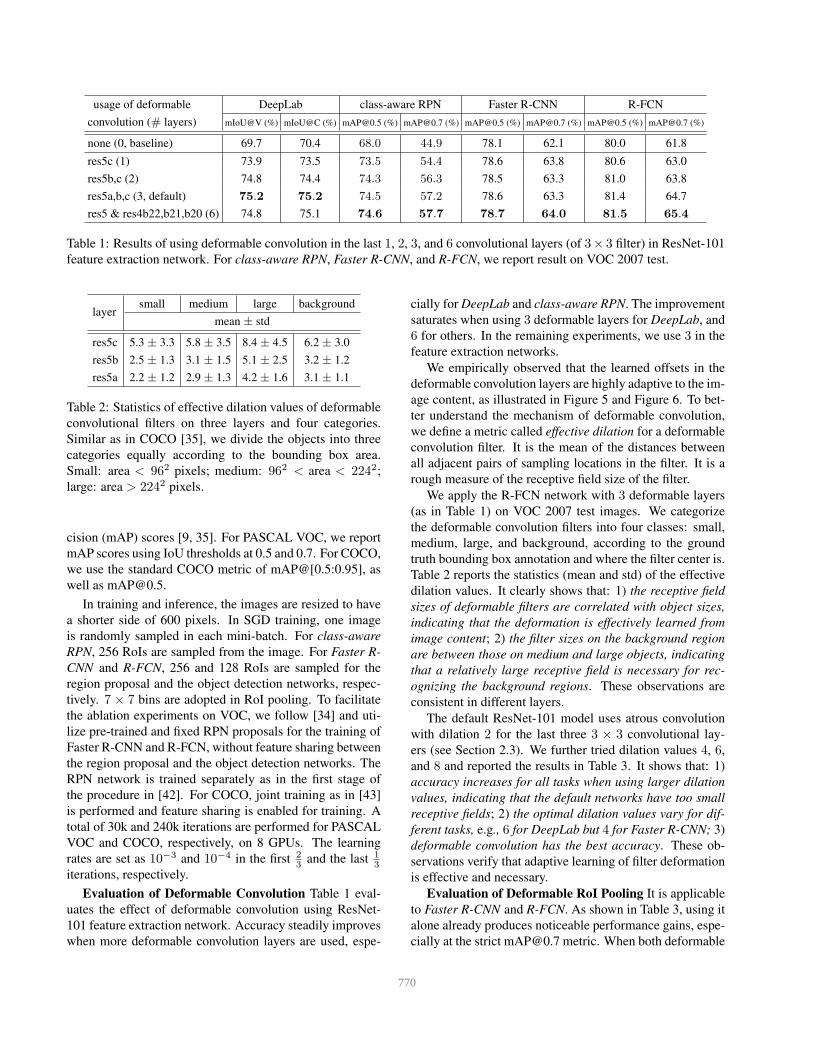
Table 1: Results of using deformable convolution in the last 1, 2, 3, and 6 convolutional layers (of 3× 3 filter) in ResNet-101

feature extraction network. For class-aware RPN, Faster R-CNN, and R-FCN, we report result on VOC 2007 test.

layersmall medium large background

mean ± std

res5c 5.3 ± 3.3 5.8 ± 3.5 8.4 ± 4.5 6.2 ± 3.0

res5b 2.5 ± 1.3 3.1 ± 1.5 5.1 ± 2.5 3.2 ± 1.2

res5a 2.2 ± 1.2 2.9 ± 1.3 4.2 ± 1.6 3.1 ± 1.1

Table 2: Statistics of effective dilation values of deformable

convolutional filters on three layers and four categories.

Similar as in COCO [35], we divide the objects into three

categories equally according to the bounding box area.

Small: area < 962 pixels; medium: 962 < area < 2242;

large: area > 2242 pixels.

cision (mAP) scores [9, 35]. For PASCAL VOC, we report

mAP scores using IoU thresholds at 0.5 and 0.7. For COCO,

we use the standard COCO metric of mAP@[0.5:0.95], as

well as [email protected].

In training and inference, the images are resized to have

a shorter side of 600 pixels. In SGD training, one image

is randomly sampled in each mini-batch. For class-aware

RPN, 256 RoIs are sampled from the image. For Faster R-

CNN and R-FCN, 256 and 128 RoIs are sampled for the

region proposal and the object detection networks, respec-

tively. 7 × 7 bins are adopted in RoI pooling. To facilitate

the ablation experiments on VOC, we follow [34] and uti-

lize pre-trained and fixed RPN proposals for the training of

Faster R-CNN and R-FCN, without feature sharing between

the region proposal and the object detection networks. The

RPN network is trained separately as in the first stage of

the procedure in [42]. For COCO, joint training as in [43]

is performed and feature sharing is enabled for training. A

total of 30k and 240k iterations are performed for PASCAL

VOC and COCO, respectively, on 8 GPUs. The learning

rates are set as 10−3 and 10−4 in the first 23 and the last 1

3iterations, respectively.

Evaluation of Deformable Convolution Table 1 eval-

uates the effect of deformable convolution using ResNet-

101 feature extraction network. Accuracy steadily improves

when more deformable convolution layers are used, espe-

cially for DeepLab and class-aware RPN. The improvement

saturates when using 3 deformable layers for DeepLab, and

6 for others. In the remaining experiments, we use 3 in the

feature extraction networks.

We empirically observed that the learned offsets in the

deformable convolution layers are highly adaptive to the im-

age content, as illustrated in Figure 5 and Figure 6. To bet-

ter understand the mechanism of deformable convolution,

we define a metric called effective dilation for a deformable

convolution filter. It is the mean of the distances between

all adjacent pairs of sampling locations in the filter. It is a

rough measure of the receptive field size of the filter.

We apply the R-FCN network with 3 deformable layers

(as in Table 1) on VOC 2007 test images. We categorize

the deformable convolution filters into four classes: small,

medium, large, and background, according to the ground

truth bounding box annotation and where the filter center is.

Table 2 reports the statistics (mean and std) of the effective

dilation values. It clearly shows that: 1) the receptive field

sizes of deformable filters are correlated with object sizes,

indicating that the deformation is effectively learned from

image content; 2) the filter sizes on the background region

are between those on medium and large objects, indicating

that a relatively large receptive field is necessary for rec-

ognizing the background regions. These observations are

consistent in different layers.

The default ResNet-101 model uses atrous convolution

with dilation 2 for the last three 3 × 3 convolutional lay-

ers (see Section 2.3). We further tried dilation values 4, 6,

and 8 and reported the results in Table 3. It shows that: 1)

accuracy increases for all tasks when using larger dilation

values, indicating that the default networks have too small

receptive fields; 2) the optimal dilation values vary for dif-

ferent tasks, e.g., 6 for DeepLab but 4 for Faster R-CNN; 3)

deformable convolution has the best accuracy. These ob-

servations verify that adaptive learning of filter deformation

is effective and necessary.

Evaluation of Deformable RoI Pooling It is applicable

to Faster R-CNN and R-FCN. As shown in Table 3, using it

alone already produces noticeable performance gains, espe-

cially at the strict [email protected] metric. When both deformable

770

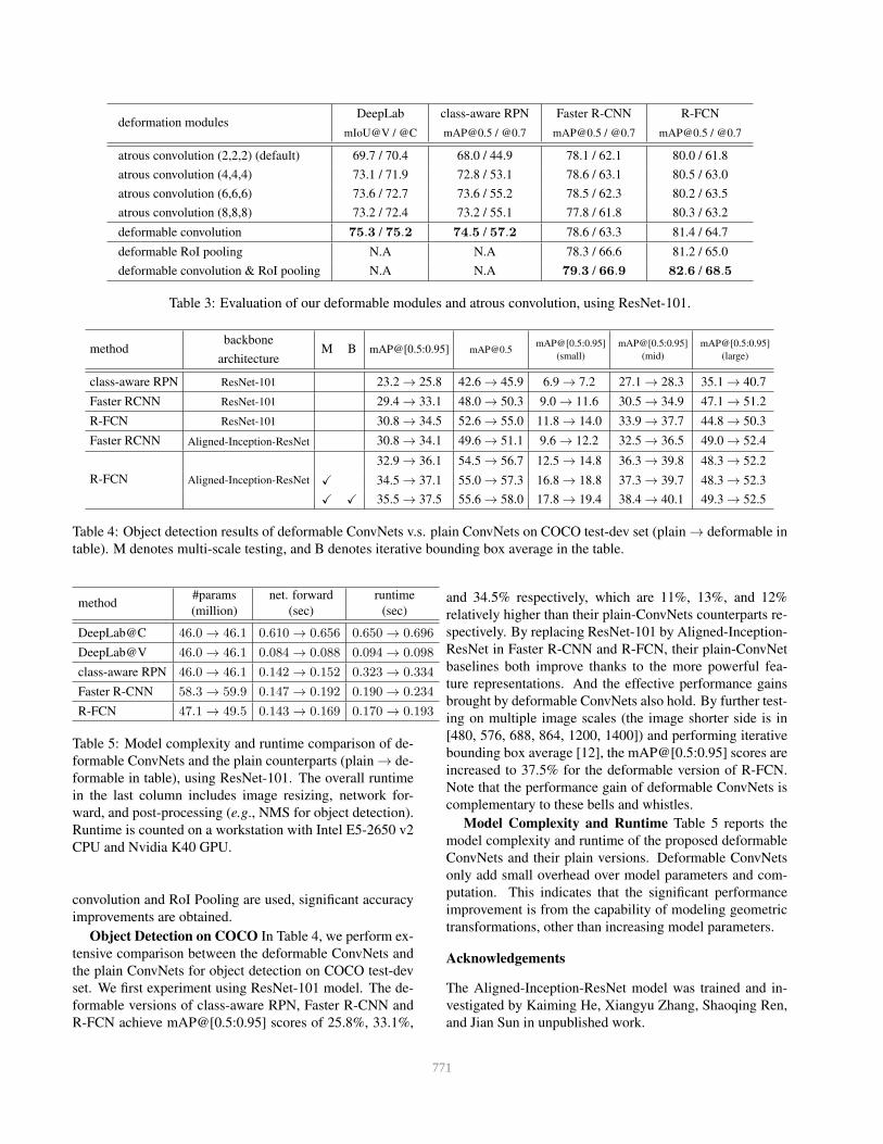
deformation modulesDeepLab

mIoU@V / @C

class-aware RPN

[email protected] / @0.7

Faster R-CNN

[email protected] / @0.7

R-FCN

[email protected] / @0.7

atrous convolution (2,2,2) (default) 69.7 / 70.4 68.0 / 44.9 78.1 / 62.1 80.0 / 61.8

atrous convolution (4,4,4) 73.1 / 71.9 72.8 / 53.1 78.6 / 63.1 80.5 / 63.0

atrous convolution (6,6,6) 73.6 / 72.7 73.6 / 55.2 78.5 / 62.3 80.2 / 63.5

atrous convolution (8,8,8) 73.2 / 72.4 73.2 / 55.1 77.8 / 61.8 80.3 / 63.2

deformable convolution 75.3 / 75.2 74.5 / 57.2 78.6 / 63.3 81.4 / 64.7

deformable RoI pooling N.A N.A 78.3 / 66.6 81.2 / 65.0

deformable convolution & RoI pooling N.A N.A 79.3 / 66.9 82.6 / 68.5

Table 3: Evaluation of our deformable modules and atrous convolution, using ResNet-101.

methodbackbone

architectureM B mAP@[0.5:0.95] [email protected]

mAP@[0.5:0.95]

(small)

mAP@[0.5:0.95]

(mid)

mAP@[0.5:0.95]

(large)

class-aware RPN ResNet-101 23.2 → 25.8 42.6 → 45.9 6.9 → 7.2 27.1 → 28.3 35.1 → 40.7

Faster RCNN ResNet-101 29.4 → 33.1 48.0 → 50.3 9.0 → 11.6 30.5 → 34.9 47.1 → 51.2

R-FCN ResNet-101 30.8 → 34.5 52.6 → 55.0 11.8 → 14.0 33.9 → 37.7 44.8 → 50.3

Faster RCNN Aligned-Inception-ResNet 30.8 → 34.1 49.6 → 51.1 9.6 → 12.2 32.5 → 36.5 49.0 → 52.4

R-FCN Aligned-Inception-ResNet

32.9 → 36.1 54.5 → 56.7 12.5 → 14.8 36.3 → 39.8 48.3 → 52.2

X 34.5 → 37.1 55.0 → 57.3 16.8 → 18.8 37.3 → 39.7 48.3 → 52.3

X X 35.5 → 37.5 55.6 → 58.0 17.8 → 19.4 38.4 → 40.1 49.3 → 52.5

Table 4: Object detection results of deformable ConvNets v.s. plain ConvNets on COCO test-dev set (plain → deformable in

table). M denotes multi-scale testing, and B denotes iterative bounding box average in the table.

method#params

(million)

net. forward

(sec)

runtime

(sec)

DeepLab@C 46.0 → 46.1 0.610 → 0.656 0.650 → 0.696

DeepLab@V 46.0 → 46.1 0.084 → 0.088 0.094 → 0.098

class-aware RPN 46.0 → 46.1 0.142 → 0.152 0.323 → 0.334

Faster R-CNN 58.3 → 59.9 0.147 → 0.192 0.190 → 0.234

R-FCN 47.1 → 49.5 0.143 → 0.169 0.170 → 0.193

Table 5: Model complexity and runtime comparison of de-

formable ConvNets and the plain counterparts (plain → de-

formable in table), using ResNet-101. The overall runtime

in the last column includes image resizing, network for-

ward, and post-processing (e.g., NMS for object detection).

Runtime is counted on a workstation with Intel E5-2650 v2

CPU and Nvidia K40 GPU.

convolution and RoI Pooling are used, significant accuracy

improvements are obtained.

Object Detection on COCO In Table 4, we perform ex-

tensive comparison between the deformable ConvNets and

the plain ConvNets for object detection on COCO test-dev

set. We first experiment using ResNet-101 model. The de-

formable versions of class-aware RPN, Faster R-CNN and

R-FCN achieve mAP@[0.5:0.95] scores of 25.8%, 33.1%,

and 34.5% respectively, which are 11%, 13%, and 12%

relatively higher than their plain-ConvNets counterparts re-

spectively. By replacing ResNet-101 by Aligned-Inception-

ResNet in Faster R-CNN and R-FCN, their plain-ConvNet

baselines both improve thanks to the more powerful fea-

ture representations. And the effective performance gains

brought by deformable ConvNets also hold. By further test-

ing on multiple image scales (the image shorter side is in

[480, 576, 688, 864, 1200, 1400]) and performing iterative

bounding box average [12], the mAP@[0.5:0.95] scores are

increased to 37.5% for the deformable version of R-FCN.

Note that the performance gain of deformable ConvNets is

complementary to these bells and whistles.

Model Complexity and Runtime Table 5 reports the

model complexity and runtime of the proposed deformable

ConvNets and their plain versions. Deformable ConvNets

only add small overhead over model parameters and com-

putation. This indicates that the significant performance

improvement is from the capability of modeling geometric

transformations, other than increasing model parameters.

Acknowledgements

The Aligned-Inception-ResNet model was trained and in-

vestigated by Kaiming He, Xiangyu Zhang, Shaoqing Ren,

and Jian Sun in unpublished work.

771

References

[1] Y.-L. Boureau, J. Ponce, and Y. LeCun. A theoretical analy-

sis of feature pooling in visual recognition. In ICML, 2010.

[2] J. Bruna and S. Mallat. Invariant scattering convolution net-

works. TPAMI, 2013.

[3] L.-C. Chen, G. Papandreou, I. Kokkinos, K. Murphy, and

A. L. Yuille. Semantic image segmentation with deep con-

volutional nets and fully connected crfs. In ICLR, 2015.

[4] L.-C. Chen, G. Papandreou, I. Kokkinos, K. Murphy, and

A. L. Yuille. Deeplab: Semantic image segmentation with

deep convolutional nets, atrous convolution, and fully con-

nected crfs. arXiv preprint arXiv:1606.00915, 2016.

[5] M. Cordts, M. Omran, S. Ramos, T. Rehfeld, M. Enzweiler,

R. Benenson, U. Franke, S. Roth, and B. Schiele. The

cityscapes dataset for semantic urban scene understanding.

In CVPR, 2016.

[6] J. Dai, Y. Li, K. He, and J. Sun. R-fcn: Object detection via

region-based fully convolutional networks. In NIPS, 2016.

[7] J. Deng, W. Dong, R. Socher, L.-J. Li, K. Li, and L. Fei-

Fei. Imagenet: A large-scale hierarchical image database. In

CVPR, 2009.

[8] S. Dieleman, J. D. Fauw, and K. Kavukcuoglu. Exploiting

cyclic symmetry in convolutional neural networks. arXiv

preprint arXiv:1602.02660, 2016.

[9] M. Everingham, L. Van Gool, C. K. Williams, J. Winn, and

A. Zisserman. The PASCAL Visual Object Classes (VOC)

Challenge. IJCV, 2010.

[10] P. F. Felzenszwalb, R. B. Girshick, D. McAllester, and D. Ra-

manan. Object detection with discriminatively trained part-

based models. TPAMI, 2010.

[11] R. Gens and P. M. Domingos. Deep symmetry networks. In

NIPS, 2014.

[12] S. Gidaris and N. Komodakis. Object detection via a multi-

region & semantic segmentation-aware cnn model. In ICCV,

2015.

[13] R. Girshick. Fast R-CNN. In ICCV, 2015.

[14] R. Girshick, J. Donahue, T. Darrell, and J. Malik. Rich fea-

ture hierarchies for accurate object detection and semantic

segmentation. In CVPR, 2014.

[15] R. Girshick, F. Iandola, T. Darrell, and J. Malik. De-

formable part models are convolutional neural networks.

arXiv preprint arXiv:1409.5403, 2014.

[16] B. Hariharan, P. Arbelaez, L. Bourdev, S. Maji, and J. Malik.

Semantic contours from inverse detectors. In ICCV, 2011.

[17] B. Hariharan, P. Arbelaez, R. Girshick, and J. Malik. Simul-

taneous detection and segmentation. In ECCV. 2014.

[18] K. He, X. Zhang, S. Ren, and J. Sun. Aligned-inception-

resnet model, unpublished work.

[19] K. He, X. Zhang, S. Ren, and J. Sun. Spatial pyramid pooling

in deep convolutional networks for visual recognition. In

ECCV, 2014.

[20] K. He, X. Zhang, S. Ren, and J. Sun. Deep residual learning

for image recognition. In CVPR, 2016.

[21] M. Holschneider, R. Kronland-Martinet, J. Morlet, and

P. Tchamitchian. A real-time algorithm for signal analysis

with the help of the wavelet transform. Wavelets: Time-

Frequency Methods and Phase Space, page 289297, 1989.

[22] J. Huang, V. Rathod, C. Sun, M. Zhu, A. Korattikara,

A. Fathi, I. Fischer, Z. Wojna, Y. Song, S. Guadarrama, and

K. Murphy. Speed/accuracy trade-offs for modern convo-

lutional object detectors. arXiv preprint arXiv:1611.10012,

2016.

[23] M. Jaderberg, K. Simonyan, A. Zisserman, and

K. Kavukcuoglu. Spatial transformer networks. In

NIPS, 2015.

[24] Y. Jeon and J. Kim. Active convolution: Learning the shape

of convolution for image classification. In CVPR, 2017.

[25] Y. Jia, C. Huang, and T. Darrell. Beyond spatial pyramids:

Receptive field learning for pooled image features. In CVPR,

2012.

[26] A. Kanazawa, A. Sharma, and D. Jacobs. Locally scale-

invariant convolutional neural networks. In NIPS, 2014.

[27] A. Krizhevsky, I. Sutskever, and G. E. Hinton. Imagenet

classification with deep convolutional neural networks. In

NIPS, 2012.

[28] D. Laptev and J. M.Buhmann. Transformation-invariant con-

volutional jungles. In CVPR, 2015.

[29] D. Laptev, N. Savinov, J. M. Buhmann, and M. Polle-

feys. Ti-pooling: transformation-invariant pooling for fea-

ture learning in convolutional neural networks. arXiv

preprint arXiv:1604.06318, 2016.

[30] S. Lazebnik, C. Schmid, and J. Ponce. Beyond bags of

features: Spatial pyramid matching for recognizing natural

scene categories. In CVPR, 2006.

[31] Y. LeCun and Y. Bengio. Convolutional networks for images,

speech, and time series. The handbook of brain theory and

neural networks, 1995.

[32] K. Lenc and A. Vedaldi. Understanding image representa-

tions by measuring their equivariance and equivalence. In

CVPR, 2015.

[33] C.-H. Lin and S. Lucey. Inverse compositional spatial trans-

former networks. arXiv preprint arXiv:1612.03897, 2016.

[34] T.-Y. Lin, P. Dollar, R. Girshick, K. He, B. Hariharan, and

S. Belongie. Feature pyramid networks for object detection.

In CVPR, 2017.

[35] T.-Y. Lin, M. Maire, S. Belongie, J. Hays, P. Perona, D. Ra-

manan, P. Dollar, and C. L. Zitnick. Microsoft COCO: Com-

mon objects in context. In ECCV. 2014.

[36] W. Liu, D. Anguelov, D. Erhan, C. Szegedy, and S. Reed.

Ssd: Single shot multibox detector. In ECCV, 2016.

[37] J. Long, E. Shelhamer, and T. Darrell. Fully convolutional

networks for semantic segmentation. In CVPR, 2015.

[38] D. G. Lowe. Object recognition from local scale-invariant

features. In ICCV, 1999.

[39] W. Luo, Y. Li, R. Urtasun, and R. Zemel. Understanding

the effective receptive field in deep convolutional neural net-

works. arXiv preprint arXiv:1701.04128, 2017.

[40] W. Ouyang, X. Wang, X. Zeng, S. Qiu, P. Luo, Y. Tian, H. Li,

S. Yang, Z. Wang, C.-C. Loy, and X. Tang. Deepid-net: De-

formable deep convolutional neural networks for object de-

tection. In CVPR, 2015.

[41] J. Redmon, S. Divvala, R. Girshick, and A. Farhadi. You

only look once: Unified, real-time object detection. In

CVPR, 2016.

772

[42] S. Ren, K. He, R. Girshick, and J. Sun. Faster R-CNN: To-

wards real-time object detection with region proposal net-

works. In NIPS, 2015.

[43] S. Ren, K. He, R. Girshick, and J. Sun. Faster R-CNN: To-

wards real-time object detection with region proposal net-

works. TPAMI, 2016.

[44] E. Rublee, V. Rabaud, K. Konolige, and G. Bradski. Orb: an

efficient alternative to sift or surf. In ICCV, 2011.

[45] K. Sohn and H. Lee. Learning invariant representations with

local transformations. In ICML, 2012.

[46] C. Szegedy, S. Ioffe, V. Vanhoucke, and A. Alemi. Inception-

v4, inception-resnet and the impact of residual connections

on learning. arXiv preprint arXiv:1602.07261, 2016.

[47] C. Szegedy, S. Reed, D. Erhan, and D. Anguelov. Scalable,

high-quality object detection. arXiv:1412.1441v2, 2014.

[48] D. E. Worrall, S. J. Garbin, D. Turmukhambetov, and G. J.

Brostow. Harmonic networks: Deep translation and rotation

equivariance. arXiv preprint arXiv:1612.04642, 2016.

[49] F. Yu and V. Koltun. Multi-scale context aggregation by di-

lated convolutions. In ICLR, 2016.

[50] F. Yu, V. Koltun, and T. Funkhouser. Dilated residual net-

works. In CVPR, 2017.

773