Deflation-based power iteration clustering - Department of Computer

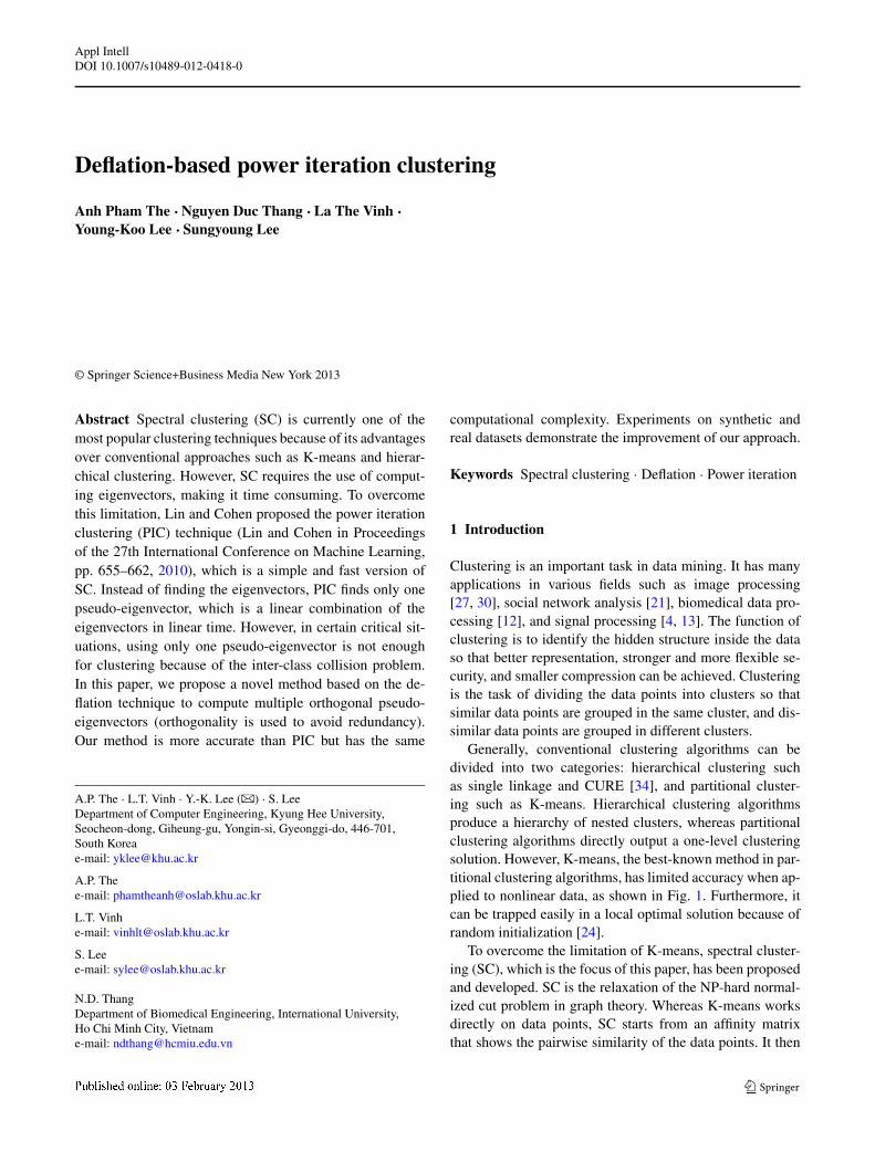
Appl IntellDOI 10.1007/s10489-012-0418-0

Deflation-based power iteration clustering

Anh Pham The · Nguyen Duc Thang · La The Vinh ·Young-Koo Lee · Sungyoung Lee

© Springer Science+Business Media New York 2013

Abstract Spectral clustering (SC) is currently one of themost popular clustering techniques because of its advantagesover conventional approaches such as K-means and hierar-chical clustering. However, SC requires the use of comput-ing eigenvectors, making it time consuming. To overcomethis limitation, Lin and Cohen proposed the power iterationclustering (PIC) technique (Lin and Cohen in Proceedingsof the 27th International Conference on Machine Learning,pp. 655–662, 2010), which is a simple and fast version ofSC. Instead of finding the eigenvectors, PIC finds only onepseudo-eigenvector, which is a linear combination of theeigenvectors in linear time. However, in certain critical sit-uations, using only one pseudo-eigenvector is not enoughfor clustering because of the inter-class collision problem.In this paper, we propose a novel method based on the de-flation technique to compute multiple orthogonal pseudo-eigenvectors (orthogonality is used to avoid redundancy).Our method is more accurate than PIC but has the same

A.P. The · L.T. Vinh · Y.-K. Lee (�) · S. LeeDepartment of Computer Engineering, Kyung Hee University,Seocheon-dong, Giheung-gu, Yongin-si, Gyeonggi-do, 446-701,South Koreae-mail: [email protected]

A.P. Thee-mail: [email protected]

L.T. Vinhe-mail: [email protected]

S. Leee-mail: [email protected]

N.D. ThangDepartment of Biomedical Engineering, International University,Ho Chi Minh City, Vietname-mail: [email protected]

computational complexity. Experiments on synthetic andreal datasets demonstrate the improvement of our approach.

Keywords Spectral clustering · Deflation · Power iteration

1 Introduction

Clustering is an important task in data mining. It has manyapplications in various fields such as image processing[27, 30], social network analysis [21], biomedical data pro-cessing [12], and signal processing [4, 13]. The function ofclustering is to identify the hidden structure inside the dataso that better representation, stronger and more flexible se-curity, and smaller compression can be achieved. Clusteringis the task of dividing the data points into clusters so thatsimilar data points are grouped in the same cluster, and dis-similar data points are grouped in different clusters.

Generally, conventional clustering algorithms can bedivided into two categories: hierarchical clustering suchas single linkage and CURE [34], and partitional cluster-ing such as K-means. Hierarchical clustering algorithmsproduce a hierarchy of nested clusters, whereas partitionalclustering algorithms directly output a one-level clusteringsolution. However, K-means, the best-known method in par-titional clustering algorithms, has limited accuracy when ap-plied to nonlinear data, as shown in Fig. 1. Furthermore, itcan be trapped easily in a local optimal solution because ofrandom initialization [24].

To overcome the limitation of K-means, spectral cluster-ing (SC), which is the focus of this paper, has been proposedand developed. SC is the relaxation of the NP-hard normal-ized cut problem in graph theory. Whereas K-means worksdirectly on data points, SC starts from an affinity matrixthat shows the pairwise similarity of the data points. It then

A.P. The et al.

Fig. 1 The K-means’ output onnonlinear data, and the PIC’limitation which is solved byour proposed additionalpseudo-eigenvector.(a) A 3-spiral dataset;(b) the output of K-means;(c) the pseudo-eigenvectorproduced by PIC. Thehorizontal axis represents theindexes of all data points. Thevertical axis shows therepresentative values of the datapoints in thepseudo-eigenvector. The datapoints are sorted in a sequencein which close data points are inthe same cluster. Therepresentative values of redsquare cluster and black starcluster are merged because ofthe blue triangle cluster; (d) theoutput of PIC using the PIC’pseudo-eigenvector; (e) theadditional pseudo-eigenvectorproduced by our method isorthogonal to the PIC’pseudo-eigenvector, hence thesquare cluster and the starcluster are totally separated;Using (c) and (e), the exactclustering solution (f) is found(Color figure online)

computes the Laplacian matrix from the affinity matrix andfinds the eigenvectors from this matrix. The effort requiredto compute the eigenvectors is relatively high, O(n3), wheren is the number of data points. Given the high computationalcost, several researchers have focused on developing fast SCtechniques (using the sampling method [3, 28, 32, 33, 36],the Nyström method [5, 8, 38, 39], or the power iterationmethod [16, 20]).

Among all fast SC techniques, power iteration cluster-ing (PIC) [16] is not only simple (it only requires a matrix-vector multiplication process), but is also scalable in termsof time complexity, O(n) [17]. Using the assumption [22,37] about the eigenvalues of the Laplacian matrix, instead

of finding all the k biggest eigenvectors, PIC can sim-ply and quickly compute their linear combination to con-struct a pseudo-eigenvector. Eigenvectors are mapping vec-tors that transform all data points from a linearly insep-arable domain into a linearly separable domain in whichdata points in different clusters are most weakly connected.A pseudo-eigenvector is not a member of the eigenvectorsbut is created linearly from them. Therefore, in the pseudo-eigenvector, if two data points lie in different clusters, theirvalues can still be separated. Different from the samplingmethod and the Nyström method, PIC does not modify theoriginal data distribution; thus, no information is lost. Nev-

Deflation-based power iteration clustering

ertheless, PIC has a limitation when dealing with multi-classdatasets, as shown in Fig. 1.

In this paper, we propose a novel algorithm that has bet-ter accuracy than PIC in multi-class datasets and is nearlyequal in accuracy to that of the original implementation ofSC. More importantly, the computational time of our algo-rithm is significantly smaller than that of the fast imple-mentation of SC (i.e., SCIRAM [14]). Our contributionsare twofold. First, by using the deflation method, insteadof finding only one pseudo-eigenvector similar to PIC, wefind additional pseudo-eigenvectors with interesting proper-ties. Similar to the PIC’ pseudo-eigenvector, each containsuseful information for clustering. Pseudo-eigenvectors canbe used together, and they are non-redundant because theyare mutually orthogonal. Moreover, the computational timefor finding each pseudo-eigenvector is as small as that forfinding the PIC’ pseudo-eigenvector. We also provide the-oretical proofs for these properties. Second, we justify ourmethod by conducting experiments on various handwrittendigit, human face, document, and synthetic datasets. Specif-ically, in clustering the sci topic of a 20-newsgroup dataset,we improve the accuracy of PIC from 58 % to 69 % whilekeeping the computational time 16 times smaller than thatof SCIRAM.

The rest of the paper is organized as follows. Section 2discusses the related works. Section 3 presents the back-ground of SC and PIC along with their limitations. Sec-tion 4 outlines our algorithm, and Sect. 5 examines its per-formance. Section 6 concludes the paper and summarizesfuture research directions.

2 Related works

Sampling-based SC A large number of studies have beenconducted to reduce the computational time of SC. Most ofthese studies used the sampling method to determine somerepresentative data points over the dataset [28, 32, 33, 36].In particular, finding eigenvectors from n data points takesO(n3). However, if we use sampling, the number of repre-sentative points is k � n, and this time complexity is onlyO(k3). One of the sampling-based SC techniques is pre-sented in [36] in which Yan et al. also provide an end-to-end error analysis for the method. In the first step, they useK-means to find k centroids as k representative points. Inthe second step, SC clusters these centroids together. In thepost-processing step, each data point is classified in the samecluster with its centroid. The drawback of sampling-basedmethods is that the sampling step may not properly detectsome representative data points for nonlinear datasets.

Nyström-based SC Another branch of fast SC research isthe Nyström method [5, 8, 38, 39] that uses the rank reduc-tion technique. This framework involves three steps. First,

a sampling technique is used to select some data points. Sec-ond, by using the affinity matrix between these data pointsand all data points, the eigenvectors are found through thelow-rank approximation technique. The last step is extrap-olating these eigenvectors to a full set of data points. Typi-cally, the works are different in the first step in which the is-sue is what sampling technique to use. The Nyström-basedmethods have two drawbacks: the memory requirement ishigh because a large number of high-dimension matriceshave to be stored, and the sampling method in the first stepmay ignore all data points in a small cluster; thus, this clustercannot be detected.

Power iteration-based SC Our approach lies in the thirdbranch of fast SC algorithms. This direction is taken fromthe assumption in data distribution [22, 37] that, if thedataset has k clusters, the (k + 1)th eigenvalue of theLaplacian matrix will be considerably larger than the kth.The wider the gap is, the faster the algorithm converges.Mavroeidis et al. [20] use this assumption to build a semi-supervised power iteration-based clustering algorithm. Us-ing supervised labels for several data points from the orig-inal Laplacian matrix, they created a new Laplacian matrixwith a wider gap between the two eigenvalues. Although theconvergence time of this algorithm is significantly reduced,the drawback is the high cost of obtaining supervised labels.

Dominant set clustering Similar to SC, dominant set clus-tering [23] is a well-known clustering technique that utilizesthe affinity matrix. Specifically, from the affinity matrix,without a normalization step like SC, dominant set cluster-ing iteratively updates a vector that can be used to sequen-tially filter out the most compact clusters. Generally, similarto the rare class analysis [10], the dominant set method iseffective in finding a strongly connected cluster even whenit overlaps with other clusters. PIC, without the normaliza-tion step, can also be used to sequentially detect rare classes.However, we do not focus on this modified version of PIC inthis paper. The limitation of the dominant set method is thatonly excessively compact data points can be obtained insidethe compact clusters [23].

3 Background

3.1 Spectral clustering

Assuming that we have a set of vectors X = {xi}ni=1 andeach xi is in Rd space, which represents a data point in adataset, we define a similarity function s(xi ,xj ) to show thesimilarity between xi and xj . A matrix A = {aij }ni,j=1, andeach aij = s(xi ,xj ), is called an affinity matrix. We definean affinity graph G as an undirected graph in which a vertex

A.P. The et al.

Fig. 2 PIC result for a datasetof 3 classes in Fig. 1. (a) is theinitialization vector. (b) is theiterative vector after 55iterations. (c) is the iterativevector after 108 iterations. (d) isthe constant vector after 5,000iterations. Around the 108thiteration is the localconvergence phase. Around the5,000th iteration is the globalconvergence phase. Thetransition from the initializationto the local convergence phaseis rapid (107 iterations), but thetransition from the localconvergence phase to the globalconvergence phase is very slow(4,892 iterations)

vi representing the data point xi . The weight of the edge be-tween vi and vj represents the similarity between xi and xj .The affinity matrix and the affinity graph can be sparse ifwe consider only the similarity between a data point xi andits t nearest neighbors while setting the similarity betweenxi and the others to zero. We define the diagonal matrix D,with Dii = ΣjAij , and the normalized affinity matrix W ,with W = D−1A. The Laplacian matrix is computed basedon L = I − W , where I is the unit matrix.

The goal of SC is to divide the data into groups in whichthe data points in each group have a similar property. SC hasseveral versions [22], but we focus only on the normalizedcut version in which SC is a relaxation of the normalized cutproblem in graph G. We find the k smallest eigenvectors ofL, which are also the k largest eigenvectors of W . Hereafter,when we say k eigenvectors, we refer to the k largest eigen-vectors of W . Based on these eigenvectors, we use K-meansto obtain the final SC result.

3.2 Power iteration clustering

Instead of computing k individual eigenvectors, PIC findsonly one pseudo eigenvector, which is a linear combina-tion of the eigenvectors. Power iteration, a method to com-pute the largest eigenvector of W , is the main technique inPIC. This section describes the process of finding the largesteigenvector of W and uses this process to find the pseudo-eigenvector.

Initially, an iterative vector is set as equal to the randominitialization vector v0. In each iteration, the iterative vectoris updated based on the multiplication of W with itself. Toprevent the vector from becoming too large in each iteration,we need a normalization step. Specifically,

vt = W ∗ vt−1, (1)

vt = vt /∥∥vt

∥∥, (2)

where vt is the iterative vector. If there is no change betweentwo continuous iterations, the iterative vector converges tothe largest eigenvector of W . However, because W is a nor-malized matrix, its largest eigenvector is a constant vectorthat is useless for clustering [16]. Fortunately, Lin et al. [16]found that the aforementioned iteration process to becomethe largest eigenvector of W has two phases, as illustrated inFig. 2.

• In the first phase, if two data points are in different clus-ters, their values in the iterative vector will be far apart.Therefore, this iterative vector is useful for clustering.This phase is called the local convergence phase, whichis reached at an extremely fast pace from the beginning.

• In the second phase, the iterative vector slowly becomesthe largest eigenvector, which is a constant vector. At thistime, the iterative vector is useless. This phase is calledthe global convergence phase, which is reached at an ex-tremely slow pace from the local convergence phase.

Deflation-based power iteration clustering

Algorithm 1 Power iterationInput: Normalized Affinity Matrix W .repeat

vt+1 = (Wvt )/‖Wvt‖1.σ t+1 = |vt+1 − vt |.acceleration = ‖σ t+1 − σ t‖.Increase t .

until acceleration < ε

Output: Pseudo-eigenvector vt .

To determine when the local convergence phase shouldstop, [16] computed acceleration. When the accelerationis smaller than the predefined threshold, the iteration pro-cess is stopped. The most interesting property of the iter-ative vector, if we stop the iteration process at the end ofthe local phase, is its being a linear combination of the k

largest eigenvectors of W [16]. Therefore, we call this vec-tor the pseudo-eigenvector. The details of the power iterationof PIC are presented in Algorithm 1.

However, if we use PIC in the multi-class dataset, we willhave an inter-class collision problem. As reported in Figs. 1and 2, if we use the iterative vector v at the 108th iteration,we will not find which data points are in the red square clus-ter and which data points are in the black star cluster. In thefollowing section, we show our solution to overcome thisproblem. Although there are emerging trends about paralleland distributed computing, we do not particularly design ouralgorithm for the parallel or distributed environment. How-ever, such special deployment is an interesting topic for fu-ture research.

4 The proposed deflation-based power iterationclustering algorithm

Given the inter-class collision problem, we cannot useonly one pseudo-eigenvector for clustering. We need morepseudo-eigenvectors, which are not only useful for cluster-ing (i.e., they can be a linear combination of the k largesteigenvectors) but also do not contain redundant informa-tion (i.e., they can be mutually orthogonal). Moreover, asPIC is fast and requires simple computation and low mem-ory, our algorithm must retain these advantages of PIC. Toachieve this goal, we use the deflation technique and PICtogether. We call our algorithm Deflation-based Power Iter-ation Clustering (DPIC). In the following subsections, wepresent the deflation technique and then describe the workflow and properties of our algorithm.

4.1 Deflation technique

Deflation is a technique that modifies a matrix by elimi-nating the effect of a given eigenvector. After deflation, all

eigenvectors of the modified matrix are the same as those ofthe old matrix with similar eigenvalues. However, the giveneigenvector, which is used for deflation, will have a new zeroeigenvalue. Deflation is commonly used in sparse PCA [19]when determining the eigenvectors of a covariance matrix.Sequentially, we find the first eigenvector of this covariancematrix and then eliminate its effect on the matrix throughdeflation. Therefore, in the next step, the second eigenvectorthat we obtain contains non-redundant information on thefirst eigenvector.

A number of deflation techniques are used in [19] such asHotelling deflation, projection deflation, and Schur comple-ment deflation. Schur complement deflation is used in thispaper because it is the only method that can ensure that theoutputs of our algorithm are mutually orthogonal pseudo-eigenvectors.

Assuming that we have a matrix At−1 and its eigenvectorvt , the Schur complement deflation creates a new matrix At ,which is computed by the following formula:

At = At−1 − At−1vtvTt At−1

vTt At−1vt

. (3)

The eigenvalue of vt on matrix At is zero because Atvt = 0,indicating the elimination of the effect of vt on At−1 [19].

4.2 Deflation-based PIC

In this paper, we use Schur deflation to improve PIC ac-curacy while ensuring that the time and memory complex-ity does not change significantly. We propose a sequentialmethod to find k mutually orthogonal pseudo-eigenvectors,where k is the number of clusters. First, from the originalaffinity matrix W0, we still use power iteration as PIC tofind the first pseudo-eigenvector v1. Then, we apply defla-tion to eliminate the effect of v1 on W0 to obtain the sec-ond affinity matrix W1. From W1, we apply power iterationagain to obtain the second pseudo-eigenvector v2. Then, weapply deflation again to eliminate the effect of v2 on W1.This process is repeated k times. The flow of our algorithmis presented in Algorithm 2. Our algorithm has the followingproperties:

1. Each pseudo-eigenvector produced by our algorithm(v1,v2, . . . ,vk) is a linear combination of the k largesteigenvectors of the original affinity matrix W0, indicat-ing that each pseudo-eigenvector is useful in clusteringthe data. Proposition 2 proves this property.

2. These pseudo-eigenvectors are mutually orthogonal,which means that they do not contain redundant infor-mation about each other. Given the time it takes to com-pute a new pseudo-eigenvector, we do not compute newones that contain redundant information about the oldpseudo-eigenvectors (e.g., the addition of old pseudo-eigenvectors). The same idea is applied in PCA in which

A.P. The et al.

Algorithm 2 Deflation-based Power Iteration Clustering(DPIC)

Input: Normalized Affinity Matrix W .W0 = W.

repeatvl = PowerIteration(Wl−1). //Power iteration: find vl

from Wl−1

Wl = Wl−1 − Wl−1vlvTl Wl−1

vTl Wl−1vl

. //Deflation: remove the ef-

fect of vl on Wl−1

Increase l.until l > k

Use K-Means on pseudo-eigenvectors v1,v2, . . . ,vk .Output: Clusters C1,C2, . . . ,Ck .

only orthogonal principle components are found to avoidredundancy between the principle components. Proposi-tion 3 proves this property.

3. The speed of computing every pseudo-eigenvector(v2,v3, . . . ,vk) is the same as that of computing the firstpseudo-eigenvector v1. Section 4.4 justifies this property.

Note that the original normalized affinity matrix W haseigenvectors x1,x2, . . . ,xn with the corresponding eigenval-ues of λ1, λ2, . . . , λn. These eigenvalues are sorted in de-scending order. References [22, 37] show that, if we havek clusters, the first k eigenvalues will almost be equal, andthe gap between the kth and (k + 1)th eigenvalue will beextremely large. Thus, to follow the proof more easily, weassume that the first k eigenvalues are equal to λb. All theremaining eigenvalues are equal to the (k + 1)th eigenvalue,λs , which is considerably smaller than λb . (In reality, theremaining eigenvalues are significantly smaller than λs , jus-tifying the following proof.)

Moreover, note also that different datasets have differ-ent eigenvectors and eigenvalues. Nevertheless, we have toprove that the abovementioned properties are true regardlessof the datasets. Thus, we consider x1,x2, . . . ,xn, λb, λs asvariables.

Let F be a group of vectors. Each vector is a linearcombination of (x1,x2, . . . ,xk). Specifically, F = {c1x1 +c2x2 + · · · + ckxk | ∀c1, c2, . . . , ck ∈ R}.

Let G be a group of vectors. Each vector is a multipli-cation of λb with a linear combination of (x1,x2, . . . ,xk).Specifically, G = {λb(c1x1 + c2x2 + · · · + ckxk) | ∀c1, c2,

. . . , ck ∈ R}.

Proposition 1 The following conditions are true for eachloop lth of DPIC:

1. Wl−1xi ∈ G, for i ≤ k,2. Wl−1xi = λsxi , for i > k,3. vl ∈ F .

Proof We will prove this proposition by induction on l.These conditions are true for the first loop: W0xi =

λbxi ∈ G for i ≤ k; W0xi = λsxi for i > k; v1 ∈ F [16].Assuming that these three conditions are true until the lth

loop, we will prove that they are true for the (l + 1)th loop.

1. For i ≤ k

We multiply both sides of the Schur equation with xi

Wlxi = Wl−1xi − Wl−1vl

(vTl Wl−1xi

vTl Wl−1vl

)

. (4)

According to the lth loop, vl ∈ F . As a result,

vl = c1x1 + c2x2 + · · · + ckxk. (5)

We multiply both sides with Wl−1

Wl−1vl = c1Wl−1x1 + c2Wl−1x2 + · · · + ckWl−1xk. (6)

Each factor on the right side of (6) is in G so the left side isin G. Therefore,

Wl−1vl = λb(e1x1 + e2x2 + · · · + ekxk), (7)

where eh ∈ R,∀h ≤ k.Note that x1,x2, . . . ,xk are in norm 2 and are mutually

orthogonal [22], and that Wl−1 is symmetric. Therefore,from (4), (5), and (7),

Wlxi = Wl−1xi − Wl−1vl

ei

c1e1 + c2e2 + · · · + ckek

. (8)

Both factors on the right side of (8) are in G. In sum,

Wlxi ∈ G, for i ≤ k. (9)

2. For i > k

Given that Wl−1xi = λsxi for i > k, from (4),

Wlxi = λsxi − Wl−1vl

(vTl λsxi

vTl Wl−1vl

)

. (10)

Note that xi and xj are orthogonal for j ≤ k. Therefore,from (5) and (10),

Wlxi = λsxi − Wl−1vl

(0

vTl Wl−1vl

)

= λsxi . (11)

From (11), we have

Wlxi = λsxi , for i > k. (12)

3. Computing vl+1

Deflation-based power iteration clustering

According to the (l + 1)th loop of Algorithms 1 and 2, tocompute the (l + 1)th pseudo-eigenvector, we start with arandom initialization vector:

v0 = d1x1 + d2x2 + · · · + dkxk + dk+1xk+1 + · · · + dnxn,

where dh ∈ R, ∀h ≤ n.After running the power iteration on v0, where t is a large

number of iterations

vl+1 = (Wl)t (d1x1 + d2x2 + · · · + dkxk)

+ (Wl)t (dk+1xk+1 + · · · + dnxn). (13)

Considering (9), (12), we can derive the following from(13):

vl+1 = λtb × f+λt

s × (dk+1xk+1 +· · ·+dnxn), with f ∈ F.

(14)

Note that λts � λt

b , with t being large. The coefficient λtb will

disappear after the normalizing step in Algorithm 1. There-fore, vl+1 ≈ f and vl+1 ∈ F . �

Proposition 2 Each pseudo-eigenvector produced by ouralgorithm is a linear combination of the k largest eigenvec-tors of the original affinity matrix.

Proof The proof is straightforward based on the third con-dition of Proposition 1. �

Proposition 3 The pseudo-eigenvectors produced by our al-gorithm are mutually orthogonal.

Proof From the Schur equation on the lth loop of Algo-rithm 2, we obtain

Wl = Wl−1 − Wl−1vlvTl Wl−1

vTl Wl−1vl

.

We multiply both sides with vl

Wlvl = Wl−1vl − Wl−1vlvTl Wl−1vl

vTl Wl−1vl

= 0. (15)

From the Schur equation on the (l + 1)th loop of Algo-rithm 2,

Wl+1 = Wl − Wlvl+1vTl+1Wl

vTl+1Wlvl+1

.

We multiply both sides with vl . From (15), Wlvl = 0

Wl+1vl = Wlvl − Wlvl+1vTl+1(Wlvl )

vTl+1Wlvl+1

= 0. (16)

We prove this in the same manner as that in (15), (16), with∀s ≥ l + 1. Therefore, we have

Ws−1vl = 0. (17)

From Algorithm 2, the pseudo-eigenvector of the sth loop is

vs = (Ws−1)tv0, (18)

where v0 is the initialization vector and t is the number ofiterations.

Given that the Schur deflation preserves the symmetryand using (17), we obtain

vTl vs = (

vTl WT

s−1

)

(Ws−1)t−1v0 = 0. (19)

In sum, the DPIC’ pseudo-eigenvectors are mutually orthog-onal:

vTl vs = 0. �

4.3 Computational time for each DPIC’pseudo-eigenvector

In this section, we show that the speed of computing eachDPIC’ pseudo-eigenvector is the same as that of computingthe first pseudo-eigenvector. From Algorithm 2, to find the(l + 1)th pseudo-eigenvector vl+1, we perform the poweriteration on affinity matrix Wl . Similarly, to find the firstpseudo-eigenvector v1, we perform the power iteration onaffinity matrix W0. The structure of Wl is different from thatof W0, however, we will show that it takes the same time torun the power iteration on them.

In general, the main computing cost of the power itera-tion comes from a number of matrix-vector multiplicationsteps between the affinity matrix and the current iterativevector. Therefore, first, we show that the computational timefor each step between Wl and the iterative vector is equal tothat between W0 and the iterative vector in Sect. 4.3.1. Sec-ond, we show that the number of steps for Wl is equal to thatfor W0 in Sect. 4.3.2.

4.3.1 Computational time for each step of power iterationfor each DPIC’ pseudo-eigenvector

This section shows that the time to perform a matrix-vectormultiplication step between Wl and an iterative vector isequal to that between W0 and the iterative vector. In Algo-rithm 2, although W0 is sparse, all the other matrices fromthe second loop are not. Consider the Schur complement for-mula again:

Wl = Wl−1 − Wl−1vlvTl Wl−1

vTl Wl−1vl

.

A.P. The et al.

Indeed, even if W0 is sparse, W1,W2, . . . ,Wl are not. Weneed O(n2) for a matrix-vector multiplication step if the ma-trix is dense. However, if the matrix is sparse, this step willonly take O(tn) with t as the number of non-zero items inone row of the matrix on average. W1 has two parts: thesparse matrix W0 and the multiplication of two vectors:

p = W0v1

vT1 W0v1

, qT = vT1 W0.

Even if W1 is not sparse, we can perform the matrix-vector multiplication on it quickly. Let us refer to the cur-rent iterative vector as vc. Specifically, instead of multiply-ing W1vc directly, we compute two factors W0vc and pqT vc

then perform subtraction:

W1vc = W0vc − W0v1vT1 W0

vT1 W0v1

vc = W0vc − pqT vc.

The computational time of pqT vc is O(n). The computa-tional time of W0vc is O(tn). In this manner, the computa-tional time for the W1vc multiplication is only O((t + 1)n)

≈ O(tn), which is almost equal to the computational timefor the W0vc multiplication. Based on this analysis, even ifthe new affinity matrix is not sparse, after deflation, we canguarantee that the speed of the matrix-vector multiplicationbetween the new affinity matrix and the iterative vector re-mains unchanged.

4.3.2 Number of iterations for computing each DPIC’pseudo-eigenvector

In this section, we point out that the number of matrix-vectormultiplication steps for computing each of our pseudo-eigenvectors is equal to that of the first pseudo-eigenvector.In other words, the number of iterations, t , for performingthe power iteration on the lth loop of Algorithm 2 is equalto that in the first loop, ∀l ≥ 2.

From (14), vl = λtb × f + λt

s × (dk+1xk+1 + · · · + dnxn),∀l ≥ 1. Therefore, on the one hand, in the first loop, l = 1,we can stop the iteration process with a sufficiently largevalue of t to remove the second factor, as λt

s � λtb. On

the other hand, in the lth loop, the value of t is equal tothat of the first loop because it is enough to make λt

s � λtb .

Specifically, this value of t is chosen when the accelerationis small, as in Algorithm 1. Therefore, we need the samenumber of matrix-vector multiplication steps to find everypseudo-eigenvector even though the matrices in each loopare mutually different.

4.4 Time and space complexity of DPIC

As proved in Sect. 4.3, the computational time for eachof our pseudo-eigenvectors is equal to PIC’, which is

O(n) [17]. Therefore, according to Algorithm 2, for adataset having k classes, our algorithm computes k pseudo-eigenvectors, with an overall time complexity of O(nk).Currently, alongside the original SC, which is cubic intime, is a fast implementation using the Implicitly RestartedArnoldi Method (SCIRAM), with a time complexity ofO(n2) [17]. Therefore, our algorithm is faster than SCI-RAM and SC in general because the number of classes k ismuch smaller than the number of data points n.

Our memory complexity is linear in space. To computepseudo-eigenvectors, first, we need to store one sparse ma-trix whose size is O(nt), where t is the number of neighborsfor each data point. The sparse matrix is updated to computeeach pseudo-eigenvector. Second, we need to store one it-erative vector that is O(n) in size. Third, two intermediatevectors p and q, which cost O(2n), should be stored for eachpseudo-eigenvector. Therefore, the total memory required tocompute k pseudo-eigenvectors is O(n(t + 2k + 1)), wheret and k are small with respect to n. In our experiments, onaverage, n, t , and k are 3123, 10.71, and 5.14, respectively.

5 Experiments

In this section, we conduct various experiments on realisticand synthetic datasets to empirically justify the advantagesin speed and accuracy of our algorithm over some conven-tional implementations of SC. Our computing system is In-tel Core i5 2.53 GHz, 2 GB of RAM, Matlab R2008a, andWindows 7. We compare DPIC with PIC and two versions ofSC. The first version is the original implementation SC [22]which finds all eigenvectors and then selects k eigenvectorswith the largest eigenvalues. The second version is the fastimplementation SC called SCIRAM [14]. SCIRAM directlyapproximates k eigenvectors without finding all eigenvec-tors. Hence, the computational time of the second version issignificantly smaller than that of the first version. The fol-lowing sections will briefly introduce these datasets.

5.1 Datasets

We use document, human face, and handwritten digitdatasets in our experiments to test our algorithm over a widerange of domains. These datasets are as follows:

• The first dataset is the USPS handwritten digit [31] thatcontains 9,298 images, each of which has a handwrittendigit from 0 to 9. Every image in this dataset measures16 × 16 pixels. Therefore, each image is modeled by a256-attribute vector. We use three datasets from USPS.The first is USPS49 that contains 4 and 9 digit images;the second is USPS3568 that contains 3, 5, 6, and 8 digitimages; the third is USPS0127 that contains 0, 1, 2, and 7digit images.

Deflation-based power iteration clustering

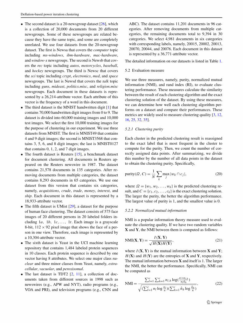
• The second dataset is a 20-newsgroup dataset [26], whichis a collection of 20,000 documents from 20 differentnewsgroups. Some of these newsgroups are related be-cause they have the same topic, and some are completelyunrelated. We use four datasets from the 20-newsgroupdataset. The first is Newsa that covers the computer topicincluding ms-windows, ibm-hardware, mac-hardware,and window-x newsgroups. The second is Newsb that cov-ers the rec topic including autos, motorcycles, baseball,and hockey newsgroups. The third is Newsc that coversthe sci topic including crypt, electronics, med, and spacenewsgroups. The last is Newsd that covers the talk topicincluding guns, mideast, politics.misc, and religion.miscnewsgroups. Each document in these datasets is repre-sented by a 26,214-attribute vector. Each attribute of thisvector is the frequency of a word in this document.

• The third dataset is the MNIST handwritten digit [1] thatcontains 70,000 handwritten digit images from 0 to 9. Thedataset is divided into 60,000 training images and 10,000test images. We select the first 10,000 training images forthe purpose of clustering in our experiment. We use threedatasets from MNIST. The first is MNIST49 that contains4 and 9 digit images; the second is MNIST3568 that con-tains 3, 5, 6, and 8 digit images; the last is MNIST0127that contains 0, 1, 2, and 7 digit images.

• The fourth dataset is Reuters [15], a benchmark datasetfor document clustering. All documents in Reuters ap-peared on the Reuters newswire in 1987. The datasetcontains 21,578 documents in 135 categories. After re-moving documents from multiple categories, the datasetcontains 8,293 documents in 65 categories. We use onedataset from this version that contains six categories,namely, acquisitions, crude, trade, money, interest, andship. Each document in this dataset is represented by a18,933-attribute vector.

• The fifth dataset is UMist [29], a dataset for the purposeof human face clustering. The dataset consists of 575 faceimages of 20 different persons in 20 labeled folders in-cluding 1a, 1b, 1c, . . . , 1t . Each image is a grayscale8-bit, 112 × 92 pixel image that shows the face of a per-son in one view. Therefore, each image is represented bya 10,304-attribute vector.

• The sixth dataset is Yeast in the UCI machine learningrepository that contains 1,484 labeled protein sequencesin 10 classes. Each protein sequence is described by onevector having 8 attributes. We select one major class nu-clear and three minor classes from Yeast, namely, extra-cellular, vacuolar, and peroxisomal.

• The last dataset is TDT2 [2, 11], a collection of doc-uments taken from different sources in 1998 such asnewswires (e.g., APW and NYT), radio programs (e.g.,VOA and PRI), and television programs (e.g., CNN and

ABC). The dataset contains 11,201 documents in 96 cat-egories. After removing documents from multiple cat-egories, the remaining documents total to 9,394 in 30categories. We select 4,981 documents in six categorieswith corresponding labels, namely, 20015, 20002, 20013,20070, 20044, and 20076. Each document in this datasetis represented by a 36,771-attribute vector.

The detailed information on our datasets is listed in Table 1.

5.2 Evaluation measure

We use three measures, namely, purity, normalized mutualinformation (NMI), and rand index (RI), to evaluate clus-tering performance. These measures calculate the similaritybetween the result of each clustering algorithm and the exactclustering solution of the dataset. By using these measures,we can determine how well each clustering algorithm per-forms on a dataset and compare their performances. Thesemetrics are widely used to measure clustering quality [3, 12,16, 25, 32, 35].

5.2.1 Clustering purity

Each cluster in the predicted clustering result is reassignedto the exact label that is most frequent in the cluster tocompute for the purity. Then, we count the number of cor-rectly assigned data points. After summarizing, we dividethis number by the number of all data points in the datasetto obtain the clustering purity. Specifically,

purity(Ω,C) = 1

N

∑

k

maxj

|wk ∩ cj |, (20)

where Ω = {w1,w2, . . . ,wk} is the predicted clustering re-sult, and C = {c1, c2, . . . , ck} is the exact clustering solution.The larger the purity, the better the algorithm performance.The largest value of purity is 1, and the smallest value is 0.

5.2.2 Normalized mutual information

NMI is a popular information theory measure used to eval-uate the clustering quality. If we have two random variablesX and Y, the NMI between them is computed as follows:

NMI(X,Y) = I (X,Y)√H(X)H(Y)

, (21)

where I (X,Y) is the mutual information between X and Y;H(X) and H(Y) are the entropies of X and Y, respectively.The mutual information between X and itself is 1. The largerthe NMI, the better the performance. Specifically, NMI canbe computed as

NMI =∑c

l=1∑c

h=1 nl,h log(n×nl,h

nl nh)

√

(∑c

l=1 nl log nl

n)(

∑ch=1 nh log nh

n)

, (22)

A.P. The et al.

Table 1 Detailed information on our datasets. For each dataset, the number of data points n, the data dimensionality d , the number of classes c,the class distribution, and the class label are provided

Dataset n d c Class distribution Class label

USPS0127 4,543 256 4 1,553/1,269/929/792 0/1/2/7

USPS3568 3,082 256 4 824/716/834/708 3/5/6/8

USPS49 1,673 256 2 852/821 4/9

MNIST0127 4,189 784 4 1,001/1,127/991/1,070 0/1/2/7

MNIST3568 3,853 784 4 1,032/863/1,014/944 3/5/6/8

MNIST49 1,958 784 2 980/978 4/9

Newsa 3,918 26,214 4 985/982/963/988 ms-windows/ibm-hardware/mac-hardware/window-x

Newsb 3,979 26,214 4 990/996/994/999 autos/motorcycles/baseball/hockey

Newsc 3,952 26,214 4 991/984/990/987 crypt/electronics/med/space

Newsd 3,253 26,214 4 910/940/775/628 guns/mideast/politics.misc/religion.misc

Reuters 3,258 18,933 6 2,055/321/298/245/197/142

acquisitions/crude/trade/money/interest/ship

TDT2 4,981 36,771 6 1,828/1,222/811/441/407/272

20015/20002/20013/20070/20044/20076

Yeast 514 8 4 429/35/30/20 nuclear/extracellular/vacuolar/peroxisomal

UMist 575 10,304 20 38/35/26/24/26/23/19/22/20/32/34/34/26/30/19/26/26/33/48/34

1a/1b/1c/1d/1e/1f/1g/1h/1i/1j/1k/1l/1m/1n/1o/1p/1q/1r/1s/1t

where nl is the number of data points in cluster ωl of thepredicted clustering result, nh is the number of data pointsin cluster ch of the exact clustering solution, and nl,h is thenumber of data points in the intersection between cluster ωl

and cluster ch.

5.2.3 Rand index

RI is a measure used to compute clustering quality based oncounting the pair of data points that both the predicted clus-tering result and the exact clustering solution agree and dis-agree that the two data points are in the same cluster. Specif-ically, we assume that the exact clustering solution of thedataset is C and that the predicted clustering result of thedataset is Ω . If the size of the dataset is N , then the numberof data pairs is N(N − 1)/2. Assume that N00 is the num-ber of pairs that are in different clusters in both C and Ω andthat N11 is the number of pairs that are in the same clusterin both C and Ω . RI can be computed as follows:

RI = 2 × (N00 + N11)

N(N − 1). (23)

The larger the RI, the better the clustering result.

5.3 Parameter setting and experiment process

We need to address two parameters to use SC as mentionedin Sect. 2. The first parameter is k, the number of classes,which is required for all algorithms including PIC, DPIC,SC, SCIRAM, and K-means. We manually set this parame-ter to the true number of classes for each dataset.

The second parameter is t , the number of neighbors foreach data point. If t is too small, the connectivity inside eachcluster may be lost. Otherwise, if t is too large, separate clus-ters may be merged. Therefore, we describe how to chooset as follows. For each dataset, we perform a pre-experimentby running SC with t selected from {5, 15, 25, 35, 45, 55,65, 75}. Then, we select the value of t which maximizes thepurity result of SC. Finally, with selected t , we report thecomputational time, purity, NMI, and RI for remaining al-gorithms. The details of the experiments when t is varied forSC are shown in Fig. 3. The performances of all algorithmswith the optimal t are reported in Tables 2, 3, 4, and 5.

In all the experiments, we use the cosine measure thatcalculates the similarity between two data points xi and xj

as follows:

s(xi ,xj ) = xTi .xj

‖xi‖‖xj‖ . (24)

Deflation-based power iteration clustering

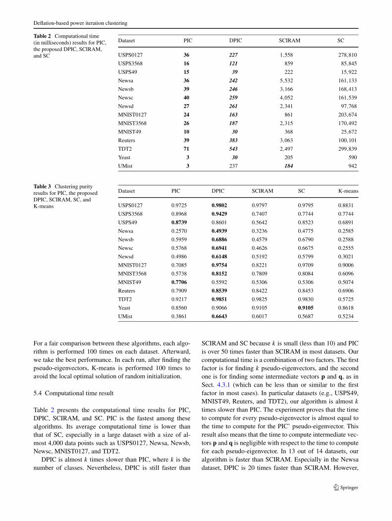
Table 2 Computational time(in milliseconds) results for PIC,the proposed DPIC, SCIRAM,and SC

Dataset PIC DPIC SCIRAM SC

USPS0127 36 227 1,558 278,810

USPS3568 16 121 859 85,845

USPS49 15 39 222 15,922

Newsa 36 242 5,532 161,133

Newsb 39 246 3,166 168,413

Newsc 40 259 4,052 161,539

Newsd 27 261 2,341 97,768

MNIST0127 24 163 861 203,674

MNIST3568 26 187 2,315 170,492

MNIST49 10 30 368 25,672

Reuters 39 383 3,063 100,101

TDT2 71 543 2,497 299,839

Yeast 3 30 205 590

UMist 3 237 184 942

Table 3 Clustering purityresults for PIC, the proposedDPIC, SCIRAM, SC, andK-means

Dataset PIC DPIC SCIRAM SC K-means

USPS0127 0.9725 0.9802 0.9797 0.9795 0.8831

USPS3568 0.8968 0.9429 0.7407 0.7744 0.7744

USPS49 0.8739 0.8601 0.5642 0.8523 0.6891

Newsa 0.2570 0.4939 0.3236 0.4775 0.2585

Newsb 0.5959 0.6886 0.4579 0.6790 0.2588

Newsc 0.5768 0.6941 0.4626 0.6675 0.2555

Newsd 0.4986 0.6148 0.5192 0.5799 0.3021

MNIST0127 0.7085 0.9754 0.8221 0.9709 0.9006

MNIST3568 0.5738 0.8152 0.7809 0.8084 0.6096

MNIST49 0.7706 0.5592 0.5306 0.5306 0.5074

Reuters 0.7909 0.8539 0.8422 0.8453 0.6906

TDT2 0.9217 0.9851 0.9825 0.9830 0.5725

Yeast 0.8560 0.9066 0.9105 0.9105 0.8618

UMist 0.3861 0.6643 0.6017 0.5687 0.5234

For a fair comparison between these algorithms, each algo-rithm is performed 100 times on each dataset. Afterward,we take the best performance. In each run, after finding thepseudo-eigenvectors, K-means is performed 100 times toavoid the local optimal solution of random initialization.

5.4 Computational time result

Table 2 presents the computational time results for PIC,DPIC, SCIRAM, and SC. PIC is the fastest among thesealgorithms. Its average computational time is lower thanthat of SC, especially in a large dataset with a size of al-most 4,000 data points such as USPS0127, Newsa, Newsb,Newsc, MNIST0127, and TDT2.

DPIC is almost k times slower than PIC, where k is thenumber of classes. Nevertheless, DPIC is still faster than

SCIRAM and SC because k is small (less than 10) and PICis over 50 times faster than SCIRAM in most datasets. Ourcomputational time is a combination of two factors. The firstfactor is for finding k pseudo-eigenvectors, and the secondone is for finding some intermediate vectors p and q, as inSect. 4.3.1 (which can be less than or similar to the firstfactor in most cases). In particular datasets (e.g., USPS49,MNIST49, Reuters, and TDT2), our algorithm is almost k

times slower than PIC. The experiment proves that the timeto compute for every pseudo-eigenvector is almost equal tothe time to compute for the PIC’ pseudo-eigenvector. Thisresult also means that the time to compute intermediate vec-tors p and q is negligible with respect to the time to computefor each pseudo-eigenvector. In 13 out of 14 datasets, ouralgorithm is faster than SCIRAM. Especially in the Newsadataset, DPIC is 20 times faster than SCIRAM. However,

A.P. The et al.

Table 4 NMI results for PIC,the proposed DPIC, SCIRAM,SC, and K-means

Dataset PIC DPIC SCIRAM SC K-means

USPS0127 0.9037 0.9264 0.9249 0.9244 0.7784

USPS3568 0.7536 0.8207 0.6794 0.6781 0.5188

USPS49 0.4533 0.4176 0.0121 0.4028 0.1118

Newsa 0.0205 0.2667 0.0270 0.2725 0.0324

Newsb 0.4315 0.5567 0.3103 0.5563 0.0336

Newsc 0.3872 0.5818 0.2192 0.5554 0.0312

Newsd 0.2876 0.4284 0.3035 0.4248 0.0503

MNIST0127 0.6420 0.9060 0.7466 0.8988 0.7386

MNIST3568 0.4710 0.6667 0.6002 0.6600 0.3866

MNIST49 0.2793 0.0101 0.0027 0.0027 0.0018

Reuters 0.4931 0.6704 0.6051 0.6134 0.2497

TDT2 0.8460 0.9415 0.9348 0.9368 0.3602

Yeast 0.2434 0.3752 0.3917 0.3917 0.1839

UMist 0.4760 0.7436 0.7248 0.6865 0.6554

Table 5 RI results for PIC, theproposed DPIC, SCIRAM, SC,and K-means

Dataset PIC DPIC SCIRAM SC K-means

USPS0127 0.9738 0.9803 0.9798 0.9796 0.8978

USPS3568 0.9114 0.9457 0.8110 0.8108 0.8206

USPS49 0.7795 0.7594 0.5082 0.7491 0.5716

Newsa 0.2589 0.6473 0.5702 0.6321 0.2594

Newsb 0.7409 0.8004 0.7045 0.7918 0.2606

Newsc 0.6827 0.7760 0.6620 0.7408 0.2558

Newsd 0.6264 0.7085 0.6220 0.5825 0.2781

MNIST0127 0.8160 0.9759 0.8709 0.9720 0.9073

MNIST3568 0.6433 0.8481 0.8171 0.8431 0.7114

MNIST49 0.6465 0.5070 0.5018 0.5018 0.5005

Reuters 0.7254 0.9077 0.8505 0.8508 0.6129

TDT2 0.9446 0.9863 0.9840 0.9844 0.5105

Yeast 0.5931 0.6920 0.6973 0.6973 0.4731

UMist 0.9150 0.9425 0.9312 0.9262 0.9322

in the UMist dataset, our computational time is longer thanthat of SCIRAM because the cost of computing intermediatevectors is high.

SCIRAM is faster than SC in all experiments; these al-gorithms are in the third and fourth places, respectively. Thespeed of SC depends on the number of data points, as it com-putes all eigenvectors. However, because SCIRAM quicklyapproximates k eigenvectors using some characters of thedataset, its speed also depends on the dataset structure. Forexample, even though the MNIST0127 dataset is larger thanthe MNIST3568 dataset, the computational time of SCI-RAM on MNIST0127 is lower.

5.5 Accuracy result

The accuracy of PIC is the worst among these algorithms,except K-means, in 9 out of 12 multi-class datasets (es-pecially in UMist, Reuters, MNIST0127, and Newsa) be-cause of the inter-class collision problems. The results areshown in Tables 3, 4, and 5. However, without the problem,PIC achieves better accuracy than do other algorithms intwo-class datasets (i.e., USPS49 and MNIST49). The bet-ter accuracy of PIC compared to SC is explained in [16].SC selects the k largest eigenvectors in which there may bea “bad” eigenvector. PIC computes the pseudo-eigenvector

Deflation-based power iteration clustering

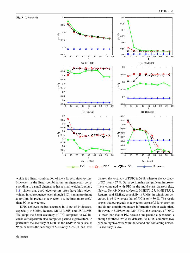
Fig. 3 Clustering purity resultsfor PIC, DPIC, SC, andK-means on realistic datasetswith different values of t

A.P. The et al.

Fig. 3 (Continued)

which is a linear combination of the k largest eigenvectors.However, in the linear combination, an eigenvector corre-sponding to a small eigenvalue has a small weight. Luxburg[18] shows that good eigenvectors often have high eigen-values. In consequence, even though PIC is an approximatealgorithm, its pseudo-eigenvector is sometimes more usefulthan SC’ eigenvectors.

DPIC achieves the best accuracy in 11 out of 14 datasets,especially in UMist, Reuters, MNIST3568, and USPS3568.We adopt the better accuracy of PIC compared to SC be-cause our algorithm also computes pseudo-eigenvectors. Inparticular, the accuracy of DPIC in the USPS3568 dataset is95 %, whereas the accuracy of SC is only 73 %. In the UMist

dataset, the accuracy of DPIC is 66 %, whereas the accuracyof SC is only 57 %. Our algorithm has a significant improve-ment compared with PIC in the multi-class datasets (i.e.,Newsa, Newsb, Newsc, Newsd, MNIST0127, MNIST3568,Reuters, and UMist), especially in UMist in which our ac-curacy is 66 % whereas that of PIC is only 39 %. The resultproves that our pseudo-eigenvectors are useful for clusteringand do not contain redundant information about each other.However, in USPS49 and MNIST49, the accuracy of DPICis lower than that of PIC because one pseudo-eigenvector isenough for these two-class datasets. As DPIC computes twopseudo-eigenvectors, with the second one containing noises,its accuracy is low.

Deflation-based power iteration clustering

Fig. 4 Clustering purity resultswith feature selection for PIC,DPIC, SC, and K-means. Notethat in the TDT2 documentsdataset, we do not report the lowresult of PIC (86 %) andK-means (63 %) in order to seethe evolution in accuracy of SCand DPIC

We also report the purity results of these algorithms onYeast, a dataset with rare classes. Generally, a rare class is aminor but compact class [10]. Our focus is to identify minorclasses, but better accuracy may come from classifying twomajor classes. Therefore, we only input one major class ofYeast. The purity result of PIC is low at 85.6 % becauseof three minor classes. Conversely, SC and DPIC achievea better solution at 90.66 % by computing multiple vectorsto solve the inter-class collision problem between the threeminor classes.

Although SCIRAM is not the best algorithm in terms ofaccuracy, it is a good approximation of SC because it isfaster while maintaining the same clustering quality. How-ever, running SCIRAM on some datasets, such as Newsa,Newsb, Newsc, and MNIST0127, is unsafe because the ac-curacy is significantly reduced.

Lastly, we report the performance of every algorithm un-der different numbers of neighbors t for each data point inFig. 3. The accuracy of our proposed DPIC is better than thatof PIC and almost similar to that of SC in almost all datasets.The accuracy of SCIRAM is the same as or lower than thatof SC in most datasets for every t so it is not reported here.Each dataset has an optimal value of t with which SC, DPIC,and PIC work best. For example, in Newsa, Newsb, and

Newsc, these algorithms achieve good results when t is 15,which is not too small or too large.

5.6 DPIC with feature selection

This section conducts experiments to determine whether theaccuracy of DPIC can be improved when incorporating fea-ture selection as a pre-processing step. Our algorithm is anunsupervised method that departs from an affinity matrixwith the similarity between data points and their local near-est neighbors. Therefore, we use the Laplacian score method[9] for the feature selection step because of its unsupervisedmanner and local neighborhood preserving advantage. Weperform experiments on three datasets USPS0127, TDT2,and especially UMist because of its huge number of features(10,304) and low number of data points (575).

In the experiments, we use a value of t with which SCworks best without the feature selection for each dataset. Atthe beginning, we use the Laplacian score to rank all featuresand then select some top-ranked features. Finally, we reportthe clustering accuracy by varying the number of selectedtop-ranked features from 20 % to 100 % of the number ofall features in the dataset, as shown in Fig. 4.

Figure 4 shows that the accuracies of SC and DPIC withthe Laplacian feature selection can be at least equal to those

A.P. The et al.

Table 6 Computational time (in milliseconds), maximum purity (MaxPurity), and average purity (AvgPurity) for the proposed DPIC and SCIRAMon synthetic graphs

Numberof nodes

SCIRAM DPIC

Time MaxPurity AvgPurity Time MaxPurity AvgPurity

10,000 Out of memory 0.000 0.000 747 1.000 1.000

9,000 Out of memory 0.000 0.000 624 1.000 1.000

8,000 Out of memory 0.000 0.000 475 1.000 1.000

7,000 Out of memory 0.000 0.000 368 1.000 1.000

6,000 Out of memory 0.000 0.000 254 1.000 1.000

5,000 17,721 0.9936 0.7700 170 1.000 1.000

4,000 9,433 0.9978 0.8608 104 1.000 1.000

3,000 5,188 1.000 0.9721 79 1.000 1.000

2,000 1,645 0.9975 0.7569 40 1.000 1.000

1,000 1,131 0.8980 0.6580 18 1.000 1.000

without feature selection. Feature selection shows its essen-tial role particularly in the UMist dataset because, if we usejust enough features (40 % to 60 %), we will achieve bet-ter accuracy than using a full set of features. Although wecannot obtain good results for the USPS0127 and TDT2datasets compared with the UMist dataset, at least we cancompress the number of features to low levels (40 % and0.8 %, respectively) while retaining equivalent accuracy.

5.7 Experiments on synthetic datasets

First, this section describes the experiments performed onsynthetic graphs to show the memory usage advantage ofour algorithm over SCIRAM. Second, we show that DPICcan achieve better accuracy than a straightforward algorithmusing k random initializations of PIC. To generate a large,sparse, and multi-class graph, we use a modified versionof Erdos, Rényi [7] random network model. The model iswidely applied to generate a synthetic network [6, 16].

5.7.1 Comparison of memory usage between DPIC andSCIRAM

We create 10 synthetic graphs, each having four clusters,with the number of nodes n ranging from 1,000 to 10,000 tocompare the memory usage of our algorithm and that of SCI-RAM. In each synthetic graph, every node connects with t

neighbor nodes when t is 2 % of n. Each cluster is a stronglyconnected cluster, as 80 % of the edges connect two nodesin the same cluster, and only 20 % of the edges connect twonodes from different clusters. In each graph, we run eachalgorithm 10 times and take the highest purity score andthe average purity score. The performances of SCIRAM andDPIC on these synthetic graphs are shown in Table 6.

SCIRAM consumes a huge amount of memory. Whenthe number of nodes is greater than 6,000, it cannot pro-duce the clustering result because of the out of memory

problem. By contrast, DPIC can perform well in all syn-thetic graphs because it stores only one sparse matrix and(2k + 1) intermediate vectors. Therefore, DPIC is linear inspace, O(n(t + 2k + 1)), where t is smaller than 200 and k

is equal to four in all graphs. Although a strong connectiv-ity exists inside every cluster, SCIRAM cannot achieve thehighest purity score. Conversely, DPIC can achieve 100 %purity in all synthetic graphs.

5.7.2 Comparison of accuracy between DPIC and k

random PIC

A straightforward solution to overcome the inter-class col-lision problem is to run PIC k times, with each time havingdifferent initialization vector v0. We call this solution thek-random PIC. The limitation of this solution is that it com-putes redundant pseudo-eigenvectors that are not mutuallyorthogonal. We create 10 synthetic graphs, with the num-ber of nodes n ranging from 1,000 to 10,000, to show thatour algorithm, which produces multiple orthogonal pseudo-eigenvectors, is more accurate than this straightforward so-lution.

We generate two groups of synthetic graphs. In the firstgroup, we set t , the number of neighbors for each node, to0.01n for all graphs. In the second group, we flexibly set t tobe equal to 0.01n for graphs having less than 3,000 nodes,0.005n for graphs having 4,000 to 6,000 nodes, and 0.002n

for graphs having more than 7,000 nodes.The purity results of DPIC and k-random PIC in the first

group are shown in Fig. 5. As we set t to be directly propor-tional to n, the number of edges increases quadratically withthe number of nodes. In consequence, the gap between thenumber of edges connecting two nodes in the same clusterand the number of edges connecting two nodes from dif-ferent clusters also increases quadratically with the numberof nodes. Therefore, finding the clustering solution for large

Deflation-based power iteration clustering

Fig. 5 Clustering purity results for DPIC and k random initializationsPIC (k-random PIC) on the first group

Fig. 6 Clustering purity results for DPIC and k random initializationsPIC (k-random PIC) on the second group

graphs that have more than 4,000 nodes seems easy. In thesegraphs, both DPIC and k-random PIC achieve best results.

The purity results of DPIC and k-random PIC in the sec-ond group are shown in Fig. 6. As we slightly decrease t

for large graphs, the number of edges does not increase toofast with respect to the number of nodes. Indeed, k-randomPIC achieves lower purity than DPIC in these cases. The re-sults experimentally show that, in difficult situations, DPICproduces a better solution than k-random PIC.

6 Conclusion

In this paper, we propose a solution to overcome theinter-class collision problem in PIC. Our method uses

the deflation technique to find more pseudo-eigenvectors.Therefore, our DPIC algorithm has better accuracy thanPIC and smaller complexity than the state-of-the-art SCI-RAM. Our method only finds mutually orthogonal pseudo-eigenvectors; therefore, the method avoids finding redun-dant pseudo-eigenvectors. Our experiments on classicaland realistic document, human face, and handwritten digitdatasets justify our idea in theory. DPIC is suitable forlarge, sparse, and multi-class datasets. However, the pseudo-eigenvectors still contain noise along with the classifica-tion information because of the method used to computepseudo-eigenvectors. After using deflation on these pseudo-eigenvectors, the inner structure of the dataset can be de-graded. In the future, we will examine how to reduce thisnoise so that the deflation has a stronger effect on PIC.

Acknowledgements This work was supported by the National Re-search Foundation of Korea (NRF) grant funded by the Korea govern-ment (MEST) (No. 2010-0013689).

References

1. Cai D Mnist dataset. URL http://www.cad.zju.edu.cn/home/dengcai/Data/MNIST/10kTrain.mat

2. Cai D Tdt2 dataset. URL http://www.cad.zju.edu.cn/home/dengcai/Data/TDT2/TDT2.mat

3. Chen X, Cai D (2011) Large scale spectral clustering withlandmark-based representation. In: Proceedings of the twenty-fifthAAAI conference on artificial intelligence, San Francisco, Califor-nia, pp 313–318

4. Chen L, Mao X, Wei P, Xue Y, Ishizuka M (2012) Mandarin emo-tion recognition combining acoustic and emotional point informa-tion. Appl Intell 37(4):602–612

5. Drineas P, Mahoney MW (2005) On the Nyström method for ap-proximating a gram matrix for improved kernel-based learning.J Mach Learn Res 6:2153–2175

6. Durrett R (2010) Some features of the spread of epidemics and in-formation on a random graph. Proc Natl Acad Sci 107(10):4491–4498

7. Erdos P, Rényi A (1960) On the evolution of random graphs. MagyTud Akad Mat Kut Intéz Közl 5:17–61

8. Fowlkes C, Belongie S, Chung F, Malik J (2004) Spectral group-ing using the Nyström method. IEEE Trans Pattern Anal MachIntell 26(2):214–225

9. He X, Cai D, Niyogi P (2005) Laplacian score for feature selec-tion. Adv Neural Inf Process Syst 18:507–514

10. He J, Tong H, Carbonell J (2010) Rare category characterization.In: Proceedings of the 10th IEEE international conference on datamining, Sydney, Australia, pp 226–235

11. Hu X, Zhang X, Lu C, Park EK, Zhou X (2009) ExploitingWikipedia as external knowledge for document clustering. In: Pro-ceedings of the 15th ACM SIGKDD international conference onknowledge discovery and data mining, Paris, France, pp 389–396

12. Jain AK (2010) Data clustering: 50 years beyond k-means. PatternRecognit Lett 31(8):651–666

13. Keshet J, Bengio S (2009) Automatic speech and speaker recog-nition: large margin and kernel methods. Wiley Online Library

14. Lehoucq RB, Sorensen DC (1996) Deflation techniques for animplicitly restarted Arnoldi iteration. SIAM J Matrix Anal Appl17(4):789–821

A.P. The et al.

15. Lewis DD Reuters-21578 dataset. URL http://www.daviddlewis.com/resources/testcollections/reuters21578/

16. Lin F, Cohen WW (2010) Power iteration clustering. In: Proceed-ings of the 27th international conference on machine learning,Haifa, Israel, pp 655–662

17. Lin F, Cohen WW (2010) A very fast method for clustering bigtext datasets. In: Proceedings of the 19th European conference onartificial intelligence, Lisbon, Portugal, pp 303–308

18. Luxburg UV (2007) A tutorial on spectral clustering. Stat Comput17(4):395–416

19. Mackey L (2008) Deflation methods for sparse pca. Adv NeuralInf Process Syst 21:1017–1024

20. Mavroeidis D (2010) Accelerating spectral clustering with partialsupervision. Data Min Knowl Discov 21(2):241–258

21. Mishra N, Schreiber R, Stanton I, Tarjan RE (2007) Clustering so-cial networks. In: Proceedings of the 5th international conferenceon algorithms and models for the web-graph, San Diego, CA, pp56–67

22. Ng AY, Jordan MI, Weiss Y (2001) On spectral clustering: analysisand an algorithm. Adv Neural Inf Process Syst 14:849–856

23. Pavan M, Pelillo M (2007) Dominant sets and pairwise clustering.IEEE Trans Pattern Anal Mach Intell 29(1):167–172

24. Peña JM, Lozano JA, Larrañaga P (1999) An empirical compari-son of four initialization methods for the k-means algorithm. Pat-tern Recognit Lett 20(10):1027–1040

25. Peng W, Li T (2011) On the equivalence between nonnegative ten-sor factorization and tensorial probabilistic latent semantic analy-sis. Appl Intell 35(2):285–295

26. Rennie J 20 newsgroups. URL http://qwone.com/~jason/20Newsgroups/

27. Saha S, Bandyopadhyay S (2011) Automatic MR brain image seg-mentation using a multiseed based multiobjective clustering ap-proach. Appl Intell 35(3):411–427

28. Shang F, Jiao LC, Shi J, Wang F, Gong M (2012) Fast affinitypropagation clustering: a multilevel approach. Pattern Recognit45(1):474–486

29. Sheffield Face database. URL http://www.sheffield.ac.uk/eee/research/iel/research/face

30. Shi J, Malik J (2000) Normalized cuts and image segmentation.IEEE Trans Pattern Anal Mach Intell 22(8):888–905

31. Smola A, Schölkopf B Datasets for benchmarks and applications.URL http://www.kernel-machines.org/data/

32. Tasdemir K (2012) Vector quantization based approximate spec-tral clustering of large datasets. Pattern Recognit 45(8):3034–3044

33. Tung F, Wong A, Clausi DA (2010) Enabling scalable spectralclustering for image segmentation. Pattern Recognit 43(12):4069–4076

34. Wu S, Chow TWS (2004) Clustering of the self-organizing mapusing a clustering validity index based on inter-cluster and intra-cluster density. Pattern Recognit 37(2):175–188

35. Wu M, Schölkopf B (2006) A local learning approach for cluster-ing. Adv Neural Inf Process Syst 19:1529–1536

36. Yan D, Huang L, Jordan MI (2009) Fast approximate spectralclustering. In: Proceedings of the 15th ACM SIGKDD interna-tional conference on knowledge discovery and data mining, Paris,France, pp 907–916

37. Zelnik-Manor L, Perona P (2004) Self-tuning spectral clustering.Adv Neural Inf Process Syst 17:1601–1608

38. Zhang K, Kwok JT (2009) Density-weighted Nyström method forcomputing large kernel eigensystems. Neural Comput 21(1):121–146

39. Zhang K, Tsang IW, Kwok JT (2008) Improved Nyström low-rankapproximation and error analysis. In: Proceedings of the 25th in-ternational conference on machine learning, Helsinki, Finland, pp1232–1239

Anh Pham The received his B.S. inComputer Science from Hanoi Uni-versity of Technology, Vietnam, in2010. He got his M.S. in ComputerEngineering from Kyung Hee Uni-versity, Korea, in 2012. His researchinterests include data mining, pat-tern recognition, and machine learn-ing.

Nguyen Duc Thang received hisB.E. degree in Computer Engineer-ing from Posts and Telecommunica-tions Institute of Technology, Viet-nam. He got his M.S. and Ph.D. de-grees in the Department of Com-puter Engineering at Kyung HeeUniversity, South Korea. His re-search interests include artificial in-telligence, computer vision, and ma-chine learning.

La The Vinh received his B.S. andM.S. from Hanoi University of Sci-ence and Technology, Vietnam, in2004 and 2007, respectively. He hascompleted his Ph.D. degree at theDepartment of Computer Engineer-ing at Kyung Hee University, Ko-rea, 2012. Currently, he is workingas a lecturer at the School of Infor-mation and Communication Tech-nology, Hanoi University of Scienceand Technology. His research inter-ests include digital signal process-ing, pattern recognition and artifi-cial intelligence.

Young-Koo Lee got his B.S., M.S.and Ph.D. in Computer Sciencefrom Korea advanced Institute ofScience and Technology, Korea.He is a professor in the Depart-ment of Computer Engineering atKyung Hee University, Korea. Hisresearch interests include ubiqui-tous data management, data mining,and databases. He is a member ofthe IEEE, the IEEE Computer Soci-ety, and the ACM.

Deflation-based power iteration clustering

Sungyoung Lee received his B.S.from Korea University, Seoul, Ko-rea. He got his M.S. and Ph.D. de-grees in Computer Science fromIllinois Institute of Technology (IIT),Chicago, Illinois, USA in 1987and 1991 respectively. He has beena professor in the Department ofComputer Engineering, Kyung HeeUniversity, Korea since 1993. Heis a founding director of the Ubiq-uitous Computing Laboratory, andhas been affiliated with a director ofNeo Medical ubiquitous-Life CareInformation Technology Research

Center, Kyung Hee University since 2006. He is a member of ACMand IEEE.