Defining Relations of Minimal Degree of the Trace Algebra of $3 \\times 3$ Matrices

$Page 1: Defining Relations of Minimal Degree of the Trace Algebra of $3 \\times 3$ Matrices$
arX

iv:m

ath/

0701

609v

1 [

mat

h.R

A]

22

Jan

2007

DEFINING RELATIONS OF MINIMAL DEGREE OF THE

TRACE ALGEBRA OF 3 × 3 MATRICES

FRANCESCA BENANTI AND VESSELIN DRENSKY

Abstract. The trace algebra Cnd over a field of characteristic 0 is generatedby all traces of products of d generic n × n matrices, n, d ≥ 2. Minimal setsof generators of Cnd are known for n = 2 and n = 3 for any d as well as forn = 4 and n = 5 and d = 2. The defining relations between the generatorsare found for n = 2 and any d and for n = 3, d = 2 only. Starting withthe generating set of C3d given by Abeasis and Pittaluga in 1989, we haveshown that the minimal degree of the set of defining relations of C3d is equalto 7 for any d ≥ 3. We have determined all relations of minimal degree. Ford = 3 we have also found the defining relations of degree 8. The proofs arebased on methods of representation theory of the general linear group and easycomputer calculations with standard functions of Maple.

Introduction

Let K be any field of characteristic 0. All vector spaces, tensor products, algebras

considered in this paper are over K. Let Xi =(

x(i)pq

)

, p, q = 1, . . . , n, i = 1, . . . , d,

be d generic n × n matrices. We consider the pure (or commutative) trace algebraCnd generated by all traces of products tr(Xi1 · · ·Xik

). The algebra Cnd coincideswith the algebra of invariants of the general linear group GLn = GLn(K) acting bysimultaneous conjugation on d matrices of size n × n. General results of invarianttheory of classical groups imply that the algebra Cnd is finitely generated. Theoryof PI-algebras provides upper bounds for the generating sets of the algebras Cnd.The Nagata-Higman theorem states that the polynomial identity xn = 0 impliesthe identity x1 · · ·xN = 0 for some N = N(n). If N is minimal with this property,then Cnd is generated by traces of products tr(Xi1 · · ·Xik

) of degree k ≤ N . Thisestimate is sharp if d is sufficiently large. A description of the defining relationsof Cnd is given by the Razmyslov-Procesi theory [17, 16] in the language of idealsof the group algebras of symmetric groups. For a background on the algebras ofmatrix invariants see, e.g. [12, 10] and for computation aspects of the theory see[9].

Explicit minimal sets of generators of Cnd and the defining relations betweenthem are found in few cases only. It is well known that, in the Nagata-Higmantheorem, N(2) = 3, N(3) = 6, and N(4) = 10, which gives bounds for the degreesof the generators of the algebras C2d, C3d, and C4d, respectively. Nevertheless, thedefining relations of Cnd are explicitly given for n = 2 and any d, see e.g. [10] for

2000 Mathematics Subject Classification. Primary: 16R30; Secondary: 16S15, 13A50, 15A72.Key words and phrases. generic matrices, matrix invariants, trace algebras, defining relations.The research of the first author was partially supported by MIUR, Italy.The research of the second author was partially supported by Grant MI-1503/2005 of the

Bulgarian National Science Fund.

1

http://arXiv.org/abs/math/0701609v1

2 FRANCESCA BENANTI AND VESSELIN DRENSKY

details, and for n = 3, d = 2, see the comments below. For n = 3, d ≥ 3 and n ≥ 4and d ≥ 2, nothing is known about the concrete form of the defining relations withrespect to fixed minimal systems of generators.

Teranishi [18] found a system of 11 generators of C32. It follows from his descrip-tion that, with respect to these generators, C32 can be defined by a single relationof degree 12. The explicit (but very complicated) form of the relation was foundby Nakamoto [15], over Z, with respect to a slightly different system of generators.Abeasis and Pittaluga [1] found a system of generators of C3d, for any d ≥ 2, interms of representation theory of the symmetric and general linear groups, in thespirit of its usage in theory of PI-algebras. Aslaksen, Drensky and Sadikova [3] gavethe defining relation of C32 with respect to the set found in [1]. Their relation ismuch simpler than that in [15]. For C42, a set of generators was found by Teranishi[18, 19] and a minimal set by Drensky and Sadikova [11], in terms of the approachin [1]. Djokovic [7] gave another minimal set of 32 generators of C42 consisting oftraces of products only. He found also a minimal set of 173 generators of C52.

As usually in invariant theory, the determination of generators and definingrelations is simpler, if one has some additional information about the algebras ofinvariants. In particular, it is very useful to know the Hilbert (or Poincare) series ofthe algebra. Again, the picture is completely clear for n = 2. The only other cases,when the Hilbert series are explicitly given, are n = 3, d = 2 (Teranishi [18]) andd = 3 (Berele and Stembridge [5]), n = 4, d = 2 (Teranishi [19] (with some typos)and corrected by Berele and Stembridge [5]). Recently Djokovic [7] has calculatedalso the Hilbert series of C52 and C62.

The minimal generating set of C3d given in [1] consists of

g = g(d) =1

240d(5d5 + 19d4 − 5d3 + 65d2 + 636)

homogeneous trace polynomials u1, . . . , ug of degree ≤ 6. In more detail, the num-ber of polynomials ui of degree k is gk, and

g1 = d, g2 =1

2(d + 1)d, g3 =

1

3d(d2 + 2), g4 =

1

24(d + 1)d(d − 1)(5d − 6),

g5 =1

30d(d − 1)(d − 2)(3d2 + 4d + 6), g6 =

1

48(d + 2)(d + 1)d(d − 1)(d2 − 3d + 4).

Hence C3d is isomorphic to the factor algebra K[y1, . . . , yg]/I. Defining deg(yi) =deg(ui), the ideal I is homogeneous. For d = 3, surprisingly, the comparison ofthe Hilbert series of C33

∼= K[y1, . . . , yg]/I given in [5], with the Hilbert series ofK[y1, . . . , yg], gives that any homogeneous minimal system of generators of the idealI contains no elements of degree ≤ 6, three elements of degree 7 and 30 elementsof degree 8. The purpose of the present paper is to find the defining relations ofminimal degree for C3d and any d ≥ 3, with respect to the generating set in [1]. Ithas turned out that the minimal degree of the relations is equal to 7 for all d ≥ 3,and there are a lot of relations of degree 7. (Compare with the single relation ofdegree 12 in the case d = 2.) The dimension of the vector space of relations ofdegree 7 is equal to

r7 = r7(d) =2

7!(d + 1)d(d − 1)(d − 2)(41d3 − 86d2 + 114d− 360).

For d = 3 we have computed also the homogeneous relations of degree 8. Thedefining relations are given in the language of representation theory of GLd. There

DEFINING RELATIONS OF 3 × 3 TRACE ALGEBRA 3

is a simple algorithm which gives the explicit form of all relations of degree 7, andof degree 8 for d = 3. The proofs involve basic representation theory of GLd anddevelop further ideas of [3, 11] and our recent paper [4] combined with computercalculations with Maple. In the case d = 3 we have used essentially the Hilbertseries of C33 from [5] which has allowed to reduce the number of computations.Our methods are quite general and we believe that they can be successfully usedfor further investigation of generic trace algebras and other algebras close to them.

1. Preliminaries

In what follows, we fix n = 3 and d ≥ 3 and denote by X1, . . . , Xd the d generic3 × 3 matrices. Often, when the value of d is clear from the context, we shalldenote C3d by C. It is a standard trick to replace the generic matrices with generictraceless matrices. We express Xi in the form

Xi =1

3tr(Xi)e + xi, i = 1, . . . , d,

where e is the identity 3 × 3 matrix and xi is a generic traceless matrix. Then

(1) C3d∼= K[tr(X1), . . . , tr(Xd)] ⊗ C0,

where the algebra C0 is generated by the traces of products tr(xi1 · · ·xik), k ≤ 6.

Hence the problem for the defining relations of C can be replaced by a similarproblem for C0.

As in the case of “ordinary” generic matrices, without loss of generality we may

replace x1 by a generic traceless diagonal matrix. Changing the variables x(i)pp , we

may assume that

(2) x1 =

x(1)11 0 0

0 x(1)22 0

0 0 −(x(1)11 + x

(1)22 )

,

(3) xi =

x(i)11 x

(i)12 x

(i)13

x(i)21 x

(i)22 x

(i)23

x(i)31 x

(i)32 −(x

(i)11 + x

(i)22 )

, i = 2, . . . , d.

Till the end of the paper we fix these d generic traceless matrices. Let C+0 = ω(C0)

be the augmentation ideal of C0. It consists of all trace polynomials f(x1, . . . , xd) ∈C0 without constant terms, i.e., satisfying the condition f(0, . . . , 0) = 0. Any min-imal system of generators of C0 lying in C+

0 forms a basis of the vector spaceC+

0 modulo (C+0 )2. Conversely, if a system of polynomials f1, . . . , fg forms a ba-

sis of C+0 modulo (C+

0 )2, and each fi is a linear combination of traces of prod-ucts tr(xi1 · · ·xik

) then it is a minimal generating system of C0. The algebraC = C3d is Z-graded assuming that the trace tr(Xi1 · · ·Xik

) is of degree k, andthis grading is inherited by C0. Similarly, C (and also C0) has a more precise Z

d-multigrading induced by the condition that X1, . . . , Xd are, respectively, of multi-degree (1, 0, . . . , 0, 0), . . . , (0, 0, . . . , 0, 1). The considerations below, stated for theZ-grading hold also for the Z

d-multigrading. The numbers g1, g2, . . . , g6 of elementsof degree 1, 2, . . . , 6, respectively, in any homogeneous minimal system of generators


is an invariant of C. Any homogeneous minimal system {f1, . . . , fh} of generatorsof C0 consists of g2, . . . , g6 elements of degree 2, . . . , 6, and h = g2 + · · ·+ g6. Hence

C0∼= K[z1, . . . , zh]/J,

with isomorphism defined by zj + J → fj, j = 1, . . . , h. If uj(z1, . . . , zh), j =1, . . . , r, is a system of generators of the ideal J , then uj(f1, . . . , fh) = 0, j =1, . . . , r, is a system of defining relations of C0 with respect to the system of gen-erators {f1, . . . , fh}. Any homogeneous system of polynomials in J (where, bydefinition deg(zj) = deg(fj)) which forms a basis of the vector space J modulo thesubspace JK[z1, . . . , zh]+, is a minimal system of generators of the ideal J . Wedenote by rk the number of elements of degree k in such a system. Clearly, rk

is the dimension of the homogeneous component of degree k of the vector spaceJ/JK[z1, . . . , zh]+.

Now we summarize the necessary background on representation theory of GLd.We refer e.g. to [14] for general facts and to [8] for applications in the spiritof the problems considered here. All GLd-modules which appear in this paperare completely reducible and are direct sums of irreducible polynomial modules.The irreducible polynomial representations of GLd are indexed by partitions λ =(λ1, . . . , λd), λ1 ≥ · · · ≥ λd ≥ 0. We denote by W (λ) = Wd(λ) the correspondingirreducible GLd-module, assuming that Wd(λ) = 0 if λd+1 6= 0. The group GLd

acts in the natural way on the d-dimensional vector space K · x1 + · · ·+ K · xd andthis action is extended diagonally on the free associative algebra K〈x1, . . . , xd〉.

The module W (λ) ⊂ K〈x1, . . . , xd〉 is generated by a unique, up to a multiplica-tive constant, homogeneous element wλ of degree λj with respect to xj , called thehighest weight vector of W (λ). It is characterized by the following property.

Lemma 1.1. Let 1 ≤ i < j ≤ d and let ∆ij be the derivation of K〈x1, . . . , xd〉defined by ∆ij(xj) = xi, ∆ij(xk) = 0, k 6= j. If w(x1, . . . , xd) ∈ K〈x1, . . . , xd〉is multihomogeneous of degree λ = (λ1, . . . , λd), then w(x1, . . . , xd) is a highest

weight vector for some W (λ) if and only if ∆ij(w(x1, . . . , xd)) = 0 for all i < j.Equivalently, w(x1, . . . , xd) is a highest weight vector for W (λ) if and only if

gij(w(x1, . . . , xd)) = w(x1, . . . , xd), 1 ≤ i < j ≤ d,

where gij is the linear operator of the d-dimensional vector space which sends xj to

xi + xj and fixes the other xk.

Proof. The lemma is a partial case of a result by De Concini, Eisenbud, and Procesi[6], see also Almkvist, Dicks, and Formanek [2]. In the version which we need, thefirst part of the lemma was established by Koshlukov [13]. The equivalence followsfrom the fact that the kernel of any locally nilpotent derivation ∆ coincides withthe fixed points of the related exponential automorphism exp(∆) = 1 + ∆/1! +∆2/2! + · · · , and gij = exp(∆ij). �

If Wi, i = 1, . . . , m, are m isomorphic copies of the GLd-module W (λ) andwi ∈ Wi are highest weight vectors, then the highest weight vector of any submoduleW (λ) of the direct sum W1 ⊕ · · · ⊕ Wm has the form ξ1w1 + · · · + ξmwm for someξi ∈ K. Any m linearly independent highest weight vectors can serve as a set ofgenerators of the GLd-module W1 ⊕ · · · ⊕ Wm.


It is convenient to work with an explicit copy of W (λ) in K〈x1, . . . , xd〉 obtainedin the following way. Let

sk(x1, . . . , xk) =∑

σ∈Sk

sign(σ)xσ(1) · · ·xσ(k)

be the standard polynomial of degree k. (Clearly,

s2(x1, x2) = x1x2 − x2x1 = [x1, x2]

is the commutator of x1 and x2.) If the lengths of the columns of the diagram of λare, respectively, k1, . . . , kp, p = λ1, then

(4) wλ = wλ(x1, . . . , xk1) = sk1

(x1, . . . , xk1) · · · skp

(x1, . . . , xkp)

is the highest weight vector of a submodule W (λ) ⊂ K〈x1, . . . , xd〉. Sometimes weshall write wλ = wλ(x1, . . . , xd), even when k1 < d.

Recall that the λ-tableau

T = (aij), aij ∈ {1, . . . , d}, i = 1, . . . , d, j = 1, . . . , λi,

is semistandard if its entries do not decrease from left to right in rows and increasefrom top to bottom in columns. The following lemma gives a basis of the vectorsubspace W (λ) ⊂ K〈x1, . . . , xd〉. It also provides an algorithm to construct thisbasis.

Lemma 1.2. Let T = (aij) be a semistandard λ-tableau such that its i-th row

contains bi,i times i, bi,i+1 times i + 1, . . ., bi,d times d. Let w(x1, . . . , xd) be the

highest weight vector of W (λ) ⊂ K〈x1, . . . , xd〉 and let

uT (x11, x12, . . . , x1d, x22, . . . , x2d, . . . , xdd)

be the multihomogeneous component of degree biq in xiq, q = i, i + 1, . . . , d, of the

polynomial

w(x11 + x12 + · · · + x1d, x22 + · · · + x2d, . . . , xdd).

When T runs on the set of semistandard λ-tableaux, the polynomials

vT = vT (x1, . . . , xd) = uT (x1, x2, . . . , xd, x2, . . . , xd, . . . , xd)

form a basis of the vector space W (λ).

Proof. By standard Vandermonde arguments, the polynomial uT (x11, x12, . . . , xdd)is a linear combination of some w(

∑α1jx1j , . . . ,

∑αdjxdj), αij ∈ K. Hence

vT (x1, . . . , xd) is a linear combination of w(∑

α1jxj , . . . ,∑

αdjxj) and belongs tothe GLd-module W (λ) generated by w(x1, . . . , xd). Without loss of generality, itis sufficient to consider the case when W (λ) is generated by the element (4). Thepolynomial w(x11+x12+· · ·+x1d, x22+· · ·+x2d, . . . , xdd) is a product of evaluations

skj(x11 + x12 + · · · + x1d, x22 + · · · + x2d, . . . , xkj ,kj

+ · · · + xkj ,d)

of standard polynomials. Hence uT (x11, x12, . . . , xdd) is a linear combination ofmonomials starting with xσ(1),q1

· · ·xσ(k1),qk1. We order the variables by x1 >

· · · > xd and consider the lexicographic order of K〈x1, . . . , xd〉. The first columnof the semistandard tableau T contains a11 < · · · < ak1 and in each row ai1 ≤ aij

for all j = 2, . . . , λi. This easily implies that the leading monomial of vT startswith xa11

xa21· · ·xak11

. Hence the first k1 variables in the leading monomial areindexed by the entries of the first column of the tableau. Continuing in the sameway, we obtain that the next k2 variables in the leading monomial are indexed with


the entries of the second row, etc. Hence, for fixed λ, the leading monomial of vT

determines completely the tableau T , and the polynomials vT are linearly indepen-dent. Since W (λ) has a basis which is in 1-1 correspondence with the semistandardλ-tableaux, and the number of vT is equal to the number of semistandard tableaux,we obtain that the polynomials vT form a basis of W (λ). �

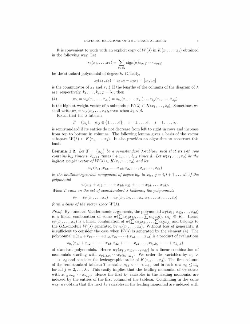
If W is a GLd-submodule or a factor module of K〈x1, . . . , xd〉, then W inheritsthe Z

d-grading of K〈x1, . . . , xd〉. Recall that the Hilbert series of W with respectto its Z

d-multigrading is defined as the formal power series

H(W, t1, . . . , td) =∑

ki≥0

dim(W (k1,...,kd))tk1

1 · · · tkd

d ,

with coefficients equal to the dimensions of the homogeneous components W (k1,...,kd)

of degree (k1, . . . , kd). It plays the role of the GLd-character of W : If

W ∼=∑

λ

m(λ)W (λ),

thenH(W, t1, . . . , td) =

∑

λ

m(λ)Sλ(t1, . . . , td),

where Sλ = Sλ(t1, . . . , td) is the Schur function associated with λ, and the mul-tiplicities m(λ) are determined by H(W, t1, . . . , td). One of the possible ways tointroduce Schur functions is via Vandermonde-like determinants. For a partitionµ = (µ1, . . . , µd), define the determinant

V (µ1, . . . , µd) =

∣∣∣∣∣∣∣∣∣

tµ1

1 tµ1

2 · · · tµ1

d

tµ2

1 tµ2

2 · · · tµ2

d...

.... . .

...tµd

1 tµd

2 · · · tµd

d

∣∣∣∣∣∣∣∣∣

.

Then the Schur function is

Sλ(t1, . . . , td) =V (λ1 + d − 1, λ2 + d − 2, . . . , λd−1 + 1, λd)

V (d − 1, d − 2, . . . , 1, 0).

The dimension of W (λ) is given by the formula

(5) dim(Wd(λ)) =∏

1≤i<j≤d

λi − λj + j − i

j − i.

The decomposition of the tensor product Wd(λ) ⊗ Wd(µ) of two irreducible GLd-modules Wd(λ) and Wd(µ) is given by the Littlewood-Richardson rule. We shallneed it in one case only:

(6) W3(22) ⊗ W3(2

2) ∼= W3(42) ⊕ W3(4, 3, 1)⊕ W3(4, 22).

But even in this case we can check the equality (6) verifying directly the equalityof symmetric functions

H(W3(22) ⊗ W3(2

2), t1, t2, t3) = S2(22)(t1, t2, t3)

= S(42)(t1, t2, t3) + S(4,3,1)(t1, t2, t3) + S(4,22)(t1, t2, t3).

In all other cases it will be sufficient to use the Young rule which is a partial caseof the Littlewood-Richardson one:

(7) Wd(λ1, . . . , λd) ⊗ Wd(p) ∼=∑

Wd(λ1 + p1, . . . , λd + pd),


where the sum runs on all nonnegative integers p1, . . . , pd such that p1+ · · ·+pd = pand λi ≥ λi+1 + pi+1, i = 1, . . . , d − 1, and its dual version

(8) Wd(λ1, . . . , λd) ⊗ Wd(1p) ∼=

∑

Wd(λ1 + ε1, . . . , λd + εd),

where the sum is on all partitions (λ1 + ε1, . . . , λd + εd) such that εi = 0, 1, ε1 +· · · + εd = p.

In the q-th symmetric tensor power

W⊗sq = W ⊗s · · · ⊗s W︸︷︷︸

q times

of the GLd-module W , we identify the tensors wσ(1)⊗· · ·⊗wσ(q) and w1⊗· · ·⊗wq,σ ∈ Sq. If W = W1 ⊕ · · · ⊕ Wk, then

(9) W⊗sq =⊕

W⊗sq1

1 ⊗ · · · ⊗ W⊗sqk

k , q1 + · · · + qk = q.

There is no general combinatorial rule for the decomposition of the symmetrictensor powers of Wd(λ). We shall need the following partial results due to Thrall[20], see also [14]:

(10) K[Wd(2)] =∑

q≥0

Wd(2)⊗sq =∑

Wd(2λ1, 2λ2, . . . , 2λd),

where the sum is over all partitions λ,

(11) Wd(p) ⊗s Wd(p) =∑

0≤k≤p/2

Wd(p + 2k, p− 2k),

(12) Wd(1p) ⊗s Wd(1p) =

∑

0≤k≤p/2

Wd(2p−2k, 14k).

Besides, we shall need the decomposition

(13) W3(22) ⊗s W (22) = W3(4

2) ⊕ W3(4, 22).

The easiest way to check (13) is to use (6), hence

W3(22) ⊗s W (22) ⊂ W3(4

2) ⊕ W3(4, 3, 1)⊕ W3(4, 22).

Therefore

W3(22) ⊗s W (22) = ε1W3(4

2) ⊕ ε2W3(4, 3, 1)⊕ ε3W3(4, 22),

εi = 0, 1. The Hilbert series of W3(22) ⊗s W3(2

2) contains the summand t41t42 and

S(42) is the only Schur function among S(42), S(4,3,1), S(4,22) which contains t41t42.

This implies that W3(42) participates in the decomposition of W3(2

2) ⊗s W3(22)

and ε1 = 1. Finally, we apply dimension arguments:

dim(W3(22) ⊗s W (22)) = dim(W3(4

2)) + ε2dim(W3(4, 3, 1)) + ε3dim(W3(4, 22)).

Since

dim(W3(22)) = 6, dim(W3(2

2) ⊗s W (22)) =

(6 + 1

2

)

= 21,

dim(W3(42)) = dim(W3(4, 3, 1)) = 15, dim(W3(4, 22)) = 6,

we obtain the only possibility ε2 = 0, ε3 = 1.The action of GLd on K〈x1, . . . , xd〉 is inherited by the algebras C3d and C0.

Now we discuss the approach of Abeasis and Pittaluga [1] for the special casen = 3. (Pay attention that the partitions in [1] are given in “Francophone” way,


i.e., transposed to ours.) The algebra C3d has a system of generators of degree ≤ 6.Without loss of generality we may assume that this system consists of traces ofproducts tr(Xi1 · · ·Xik

). Let Uk be the subalgebra of C3d generated by all tracestr(Xi1 · · ·Xil

) of degree l ≤ k. Clearly, Uk is also a GLd-submodule of C3d. Let

C(k+1)3d be the homogeneous component of degree k+1 of C3d. Then the intersection

Uk ∩ C(k+1)3d is a GLd-module and has a complement Gk+1 in C

(k+1)3d , which is the

GLd-module of the “new” generators of degree k + 1. We may assume that Gk+1

is a submodule of the GLd-module spanned by traces of products tr(Xi1 · · ·Xik+1)

of degree k + 1. The GLd-module of the generators of C3d is

G = G1 ⊕ G2 ⊕ · · · ⊕ G6.

Proposition 1.3. (Abeasis and Pittaluga [1]) The GLd-module G of the generators

of C3d decomposes as

G = W (1) ⊕ W (2) ⊕ W (3) ⊕ W (13) ⊕ W (22) ⊕ W (2, 12)

⊕W (3, 12) ⊕ W (22, 1) ⊕ W (15) ⊕ W (32) ⊕ W (3, 13).

Each module W (λ) ⊂ G is generated by the “canonical” highest weight vector

tr(wλ(X1, . . . , Xd)), where wλ is given in (4).

Corollary 1.4. The numbers gk of generators of degree k ≤ 6 in any homogeneous

minimal system of generators of C3d are

g1 = d, g2 =1

2(d + 1)d, g3 =

1

3d(d2 + 2), g4 =

1

24(d + 1)d(d − 1)(5d − 6),

g5 =1

30d(d − 1)(d − 2)(3d2 + 4d + 6), g6 =

1

48(d + 2)(d + 1)d(d − 1)(d2 − 3d + 4).

The total number of generators is

g = g(d) =1

240d(5d5 + 19d4 − 5d3 + 65d2 + 636)

Proof. The number gk is equal to the dimension of the GLd-submodule Gk of theGLd-module G of generators of C3d. Applying the formula (5) we obtain that thedimensions of the GLd-modules

W (1), W (2), W (3), W (13), W (22), W (2, 12),

W (3, 12), W (22, 1), W (15), W (32), W (3, 13).

are, respectively,

d,

(d + 1

2

)

,

(d + 2

3

)

,

(d

3

)

,d

2

(d + 1

3

)

, 3

(d + 1

4

)

,

6

(d + 2

5

)

, d

(d + 1

4

)

,

(d

5

)

, 3

(d + 2

4

)(d + 1

2

)

, 10

(d + 2

6

)

.

This easily implies the results, because

dim(G3) = dim(W (3)) + dim(W (13)), dim(G4) = dim(W (22)) + dim(W (2, 12)),

dim(G5) = dim(W (3, 12)) + dim(W (22, 1)) + dim(W (15)),

dim(G6) = dim(W (32)) + dim(W (3, 13)),

and g = g1 + g2 + · · · + g6. �


In the sequel we shall need the Hilbert series of C33 calculated by Berele andStembridge [5]:

H(C33, t1, t2, t3) =p(t1, t2, t3)

q(t1, t2, t3),

where

p = 1 − e2 + e3 + e1e3 + e22 + e2

1e3 − e2e3 − 2e1e2e3 + e23 + e2

2e3

−e21e2e3 + 2e2

1e23 + e3

1e23 + e2

2e23 − e2

1e2e23 − e1e

33 − 2e1e

22e

23

+2e2e2e33 − e3

2e23 + e3

1e33 + 2e2

1e2e33 − 2e1e

43 − e2

1e43 + e1e

22e

33

+e2e43 − e3

2e33 − 2e2

2e53 + e1e

22e

43 + 2e1e2e

53 − e6

3 − e22e

53

+e1e63 − e2e

63 − e2

1e63 − e7

3 + e1e73 − e8

3,

q =

(3∏

i=1

(1 − ti)(1 − t2i )(1 − t3i )

)

∏

1≤i<j≤3

(1 − titj)2(1 − t2i tj)(1 − tit

2j)

(1−t1t2t3),

ande1 = t1 + t2 + t3, e2 = t1t2 + t1t3 + t2t3, e3 = t1t2t3

are the elementary symmetric polynomials in three variables. Since the Hilbertseries of the tensor product is equal to the product of the Hilbert series of thefactors, and

H(K[tr(X1), . . . , tr(Xd)], t1, . . . , td) =1

(1 − t1) · · · (1 − td),

(1) implies that

H(C33, t1, t2) =H(C0, t1, t2, t3)

(1 − t1)(1 − t2)(1 − t3).

In this way, for d = 3,

(14) H(C0, t1, t2, t3) = (1 − t1)(1 − t2)(1 − t3)H(C33, t1, t2).

2. The symmetric algebra of the generators

We consider the symmetric algebra

S = K[G2 ⊕ · · · ⊕ G6]

of the GLd-module of the generators of the algebra C0. Clearly, the grading andthe GLd-module structure of G2 ⊕ · · ·⊕G6 induce a grading and the structure of aGLd-module also on S. The defining relations of the algebra C0 are in the square ofthe augmentation ideal ω(S) of S. Since we are interested in the defining relationsof degree 7 for C0 for any d ≥ 3 and of degree 8 for d = 3, we shall decomposethe homogeneous components of degree 7, respectively, 8 of the ideal ω2(S) intoa sum of irreducible GLd-, respectively, GL3-modules. Then we shall find explicitgenerators of those irreducible components which may give rise to relations.

Lemma 2.1. The following GLd-module isomorphisms hold:

(15) W (2) ⊗s W (2) ∼= W (4) ⊕ W (22),

(16) W (3) ⊗ W (2) ∼= W (5) ⊕ W (4, 1) ⊕ W (3, 2),

(17) W (13) ⊗ W (2) ∼= W (3, 12) ⊕ W (2, 13),

(18) W (22) ⊗ W (2) ∼= W (4, 2) ⊕ W (3, 2, 1) ⊕ W (23),


(19) W (2, 12) ⊗ W (2) ∼= W (4, 12) ⊕ W (3, 2, 1)⊕ W (3, 13) ⊕ W (22, 12),

(20) W (3) ⊗s W (3) ∼= W (6) ⊕ W (4, 2),

(21) W (3) ⊗ W (13) ∼= W (4, 12) ⊕ W (3, 13),

(22) W (13) ⊗s W (13) ∼= W (23) ⊕ W (2, 14),

(23) W (2) ⊗s W (2) ⊗s W (2) ∼= W (6) ⊕ W (4, 2) ⊕ W (23),

(24) W (3, 12)⊗W (2) ∼= W (5, 12)⊕W (4, 2, 1)⊕W (4, 13)⊕W (32, 1)⊕W (3, 2, 12),

(25) W (22, 1) ⊗ W (2) ∼= W (4, 2, 1)⊕ W (3, 22) ⊕ W (3, 2, 12) ⊕ W (23, 1),

(26) W (15) ⊗ W (2) ∼= W (3, 14) ⊕ W (2, 15),

(27) W (22) ⊗ W (3) ∼= W (5, 2) ⊕ W (4, 2, 1)⊕ W (3, 22),

(28) W (22) ⊗ W (13) ∼= W (32, 1) ⊕ W (3, 2, 12) ⊕ W (22, 13),

(29) W (2, 12) ⊗ W (3) ∼= W (5, 12) ⊕ W (4, 2, 1)⊕ W (4, 13) ⊕ W (3, 2, 12),

(30) W (2, 12) ⊗ W (13) ∼= W (3, 22) ⊕ W (3, 2, 12)

⊕ W (3, 14) ⊕ W (23, 1) ⊕ W (22, 13) ⊕ W (2, 15),

(31) W (3) ⊗ (W (2) ⊗s W (2)) ∼= W (7) ⊕ W (6, 1)

⊕ 2W (5, 2)⊕ W (4, 3) ⊕ W (4, 2, 1)⊕ W (3, 22),

(32) W (13) ⊗ (W (2) ⊗s W (2)) ∼= W (5, 12) ⊕ W (4, 13) ⊕ W (32, 1) ⊕ W (22, 13).

Proof. Equations (20), (22) are partial cases of (10), (11), respectively; (15) and(23) follow from (12). Equations (16), (17), (18), (19), (21), (24), (25), (26), (27),and (29) are obtained from (7); (28) and (30) follow from (8). Finally, (31) and(32) are calculated applying, respectively, (7) and (8) to (15). �

Proposition 2.2. The homogeneous components (ω2(S))(k) of degree k ≤ 7 of the

square ω2(S) of the augmentation ideal of the symmetric algebra of G2 ⊕ · · · ⊕ G6

decomposes as

(ω2(S))(4) = W (4) ⊕ W (22),

(ω2(S))(5) = W (5) ⊕ W (4, 1) ⊕ W (3, 2) ⊕ W (3, 12) ⊕ W (2, 13),

(ω2(S))(6) = 2W (6) ⊕ 3W (4, 2) ⊕ 2W (4, 12)

⊕2W (3, 2, 1)⊕ 2W (3, 13) ⊕ 3W (23) ⊕ W (22, 12) ⊕ W (2, 14),

(ω2(S))(7) = W (7) ⊕ W (6, 1) ⊕ 3W (5, 2)⊕ 3W (5, 12)

⊕W (4, 3)⊕ 5W (4, 2, 1)⊕ 3W (4, 13) ⊕ 3W (32, 1) ⊕ 4W (3, 22)

⊕6W (3, 2, 12) ⊕ 2W (3, 14) ⊕ 2W (23, 1) ⊕ 3W (22, 13) ⊕ 2W (2, 15).


Proof. By (9), the homogeneous component of degree k of ω2(S) has the form

(ω2(S))(k) =⊕

G⊗sq2

2 ⊗ · · · ⊗ G⊗sq6

6 , 2q2 + · · · + 6q6 = k, q2 + · · · + q6 ≥ 2.

The decomposition of G2, . . . , G6 is given in Proposition 1.3. Again, the equality(9) implies that (ω2(S))(k) = 0 for k < 4. For k = 4 we use (15) and obtain

(ω2(S))(4) = G2 ⊗s G2 = W (2) ⊗s W (2) = W (4) ⊕ W (22).

For k = 5, we derive

(ω2(S))(5) = G3 ⊗ G2 = (W (3) ⊕ W (13)) ⊗ W (2)

and the decomposition follows from (16) and (17). For k = 6 we have

(ω2(S))(6) = G4 ⊗ G2 ⊕ G3 ⊗s G3 ⊕ G2 ⊗s G2 ⊗s G2

and we use the decompositions given in (18) – (23). The decomposition of (ω2(S))(7)

is obtained in a similar way and makes use of (24) – (32). �

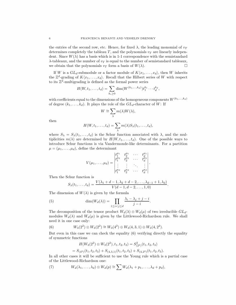
Proposition 2.3. The following elements of S = K[G2 ⊕ · · · ⊕ G6] are highest

weight vectors:

For λ = (2, 13):

w =∑

σ∈S4

sign(σ)tr(s3(xσ(1), xσ(2), xσ(3)))tr(xσ(4)x1);

For λ = (3, 13):

w1 =∑

σ∈S4

sign(σ)tr(s3(xσ(1), xσ(2), xσ(3))x1 + s3(x1, xσ(1), xσ(2))xσ(3))tr(xσ(4)x1),

w2 =∑

σ∈S4

sign(σ)tr(x21xσ(1))tr(s3(xσ(2), xσ(3), xσ(4))),

For λ = (22, 12):

w =∑

σ∈S4,τ∈S2

sign(στ)tr(s3(xσ(1), xσ(2), xσ(3))xτ(1)

+s3(xτ(1), xσ(1), xσ(2))xσ(3))tr(xσ(4)xτ(2)),

For λ = (2, 14):

w =∑

σ∈S5

sign(σ)tr(s3(xσ(1), xσ(2), xσ(3)))tr(s3(xσ(4), xσ(5), x1)).

For λ = (2, 13), (22, 12), (2, 14), every highest weight vector w ∈ W (λ) ⊂ ω2(S) is

equal, up to a multiplicative constant, to the corresponding w. For λ = (3, 13) the

highest weight vectors are linear combinations of w1 and w2.

Proof. By Proposition 1.3, the submodules W (2), W (3), W (13), W (2, 12) of G2 ⊕· · · ⊕ G6 are generated, respectively, by

v1 = tr(x21), v2 = tr(x3

1), v3 = tr(s3(x1, x2, x3)), v4 = tr(s3(x1, x2, x3)x1).

The trace polynomials tr(x1x2) and tr(s3(x1, x2, x3)x4 + s3(x2, x3, x4)x1) are lin-earizations of v1 and v4, respectively. Hence the trace polynomials w, w1, w2 de-fined in the proposition belong to the ideal ω2(S). They have the necessary skew-symmetries, as the “canonical” highest weight vectors wλ from (4). Hence all wand w1, w2 are highest weight vectors. Clearly, they are nonzero in S and theirnumber coincides with the multiplicities of W (λ) in the decomposition of ω2(S).


Hence, every highest weight vector w ∈ W (λ) ⊂ ω2(S) can be expressed as theirlinear combination. �

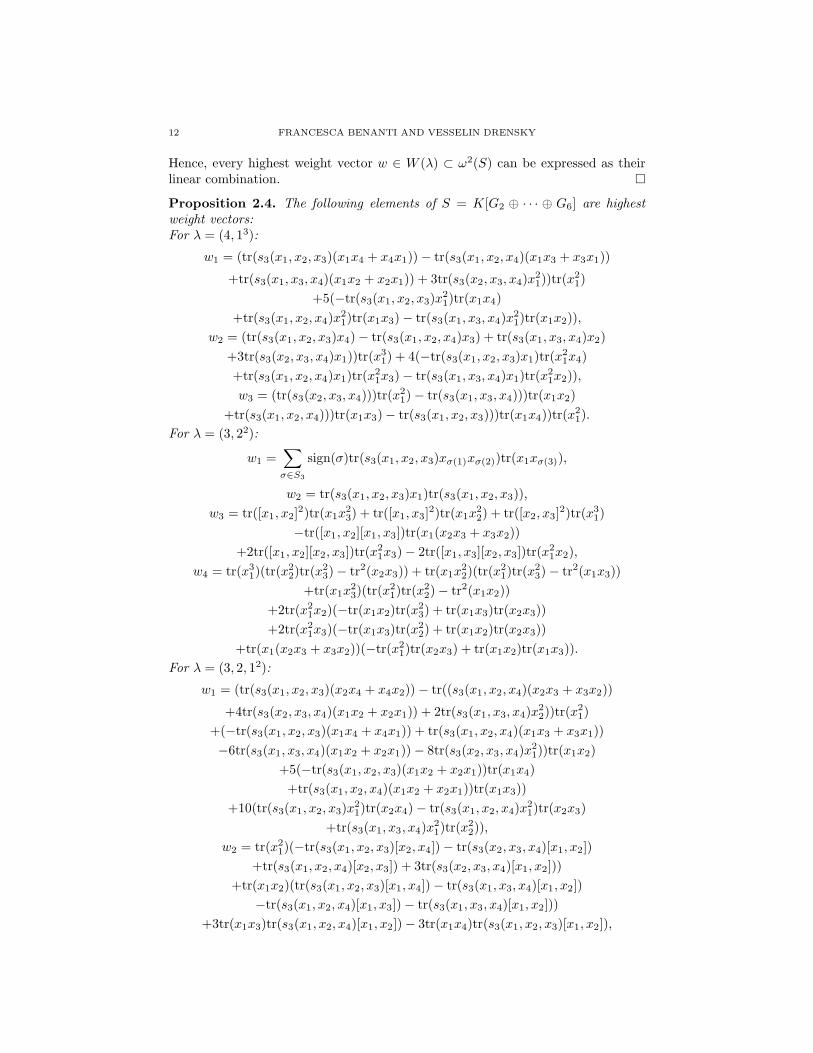
Proposition 2.4. The following elements of S = K[G2 ⊕ · · · ⊕ G6] are highest

weight vectors:

For λ = (4, 13):

w1 = (tr(s3(x1, x2, x3)(x1x4 + x4x1)) − tr(s3(x1, x2, x4)(x1x3 + x3x1))

+tr(s3(x1, x3, x4)(x1x2 + x2x1)) + 3tr(s3(x2, x3, x4)x21))tr(x

21)

+5(−tr(s3(x1, x2, x3)x21)tr(x1x4)

+tr(s3(x1, x2, x4)x21)tr(x1x3) − tr(s3(x1, x3, x4)x

21)tr(x1x2)),

w2 = (tr(s3(x1, x2, x3)x4) − tr(s3(x1, x2, x4)x3) + tr(s3(x1, x3, x4)x2)

+3tr(s3(x2, x3, x4)x1))tr(x31) + 4(−tr(s3(x1, x2, x3)x1)tr(x

21x4)

+tr(s3(x1, x2, x4)x1)tr(x21x3) − tr(s3(x1, x3, x4)x1)tr(x

21x2)),

w3 = (tr(s3(x2, x3, x4)))tr(x21) − tr(s3(x1, x3, x4)))tr(x1x2)

+tr(s3(x1, x2, x4)))tr(x1x3) − tr(s3(x1, x2, x3)))tr(x1x4))tr(x21).

For λ = (3, 22):

w1 =∑

σ∈S3

sign(σ)tr(s3(x1, x2, x3)xσ(1)xσ(2))tr(x1xσ(3)),

w2 = tr(s3(x1, x2, x3)x1)tr(s3(x1, x2, x3)),

w3 = tr([x1, x2]2)tr(x1x

23) + tr([x1, x3]

2)tr(x1x22) + tr([x2, x3]

2)tr(x31)

−tr([x1, x2][x1, x3])tr(x1(x2x3 + x3x2))

+2tr([x1, x2][x2, x3])tr(x21x3) − 2tr([x1, x3][x2, x3])tr(x

21x2),

w4 = tr(x31)(tr(x

22)tr(x

23) − tr2(x2x3)) + tr(x1x

22)(tr(x

21)tr(x

23) − tr2(x1x3))

+tr(x1x23)(tr(x

21)tr(x

22) − tr2(x1x2))

+2tr(x21x2)(−tr(x1x2)tr(x

23) + tr(x1x3)tr(x2x3))

+2tr(x21x3)(−tr(x1x3)tr(x

22) + tr(x1x2)tr(x2x3))

+tr(x1(x2x3 + x3x2))(−tr(x21)tr(x2x3) + tr(x1x2)tr(x1x3)).

For λ = (3, 2, 12):

w1 = (tr(s3(x1, x2, x3)(x2x4 + x4x2)) − tr((s3(x1, x2, x4)(x2x3 + x3x2))

+4tr(s3(x2, x3, x4)(x1x2 + x2x1)) + 2tr(s3(x1, x3, x4)x22))tr(x

21)

+(−tr(s3(x1, x2, x3)(x1x4 + x4x1)) + tr(s3(x1, x2, x4)(x1x3 + x3x1))

−6tr(s3(x1, x3, x4)(x1x2 + x2x1)) − 8tr(s3(x2, x3, x4)x21))tr(x1x2)

+5(−tr(s3(x1, x2, x3)(x1x2 + x2x1))tr(x1x4)

+tr(s3(x1, x2, x4)(x1x2 + x2x1))tr(x1x3))

+10(tr(s3(x1, x2, x3)x21)tr(x2x4) − tr(s3(x1, x2, x4)x

21)tr(x2x3)

+tr(s3(x1, x3, x4)x21)tr(x

22)),

w2 = tr(x21)(−tr(s3(x1, x2, x3)[x2, x4]) − tr(s3(x2, x3, x4)[x1, x2])

+tr(s3(x1, x2, x4)[x2, x3]) + 3tr(s3(x2, x3, x4)[x1, x2]))

+tr(x1x2)(tr(s3(x1, x2, x3)[x1, x4]) − tr(s3(x1, x3, x4)[x1, x2])

−tr(s3(x1, x2, x4)[x1, x3]) − tr(s3(x1, x3, x4)[x1, x2]))

+3tr(x1x3)tr(s3(x1, x2, x4)[x1, x2]) − 3tr(x1x4)tr(s3(x1, x2, x3)[x1, x2]),


w3 = tr([x1, x2]2)tr(s3(x1, x3, x4)) − tr([x1, x2][x1, x3])tr(s3(x1, x2, x4))

+tr([x1, x2][x1, x4])tr(s3(x1, x2, x3)),

w4 = −2tr(s3(x2, x3, x4)x2)tr(x31) + 2(tr(s3(x1, x3, x4)x2)

+tr(s3(x2, x3, x4)x1))tr(x21x2) − 2tr(s3(x1, x2, x4)x2)tr(x

21x3)

+2tr(s3(x1, x2, x3)x2)tr(x21x4) − 2tr(s3(x1, x3, x4)x1)tr(x1x

22)

+tr(s3(x1, x2, x4)x1)tr(x1(x2x3 + x3x2)) − tr(s3(x1, x2, x3)x1)tr(x1(x2x4 + x4x2)),

w5 = tr(s3(x1, x2, x3)x1)tr(s3(x1, x2, x4)) − tr(s3(x1, x2, x4)x1)tr(s3(x1, x2, x3)),

w6 = (tr(x21)tr(x

22) − tr(x1x2)

2)tr(s3(x1, x3, x4))

+(−tr(x21)tr(x2x3) + tr(x1x2)tr(x1x3))tr(s3(x1, x2, x4))

+(tr(x21)tr(x2x4) − tr(x1x2)tr(x1x4))tr(s3(x1, x2, x3)).

For λ = (3, 14):w1 = tr(s5(x1, x2, x3, x4, x5))tr(x

21),

w2 =∑

σ∈S5

sign(σ)tr(s3(x1, xσ(2), xσ(3))x1)tr(s3(x1, xσ(4), xσ(5))), σ(1) = 1.

For λ = (23, 1):w1 = tr(s3(x2, x3, x4)[x2, x3])tr(x

21)

−(tr(s3(x1, x3, x4)[x2, x3]) + tr(s3(x2, x3, x4)[x1, x3]))tr(x1x2)

+(tr(s3(x1, x2, x4)[x2, x3]) + tr(s3(x2, x3, x4)[x1, x2]))tr(x1x3)

−tr(s3(x1, x2, x3)[x2, x3])tr(x1x4) + tr(s3(x1, x3, x4)[x1, x3])tr(x22)

−(tr(s3(x1, x2, x4)[x1, x3]) + tr(s3(x1, x3, x4)[x1, x2]))tr(x2x3)

+tr(s3(x1, x2, x3)[x1, x3])tr(x2x4) + tr(s3(x1, x2, x4)[x1, x2])tr(x23)

−tr(s3(x1, x2, x3)[x1, x2])tr(x3x4),

w2 = (−3(tr(s3(x1, x2, x3)x4) + tr(s3(x2, x3, x4)x1)) + tr(s3(x1, x3, x4)x2)

+tr(s3(x2, x3, x4)x1)) − tr(s3(x1, x2, x4)x3)

+tr(s3(x2, x3, x4)x1)))tr(s3(x1, x2, x3))

+4tr(s3(x1, x2, x3)x3)tr(s3(x1, x2, x4))

−4tr(s3(x1, x2, x3)x2)tr(s3(x1, x3, x4))

+4tr(s3(x1, x2, x3)x1)tr(s3(x2, x3, x4)).

For λ = (22, 13):

w1 = (tr([x1, x4][x2, x5]) + tr([x1, x5][x2, x4])

+2tr([x1, x2][x4, x5]) − 2tr([x1, x5][x2, x4]))tr(s3(x1, x2, x3))

+(−tr([x1, x3][x2, x5]) − tr([x1, x5][x2, x3]) − 2tr([x1, x2][x3, x5])

+2tr([x1, x5][x2, x3]))tr(s3(x1, x2, x4)) + (tr([x1, x3][x2, x4])+

tr([x1, x4][x2, x3]) + 2tr([x1, x2][x3, x4])−

2tr([x1, x4][x2, x3]))tr(s3(x1, x2, x5))

+3tr([x1, x2][x2, x5])tr(s3(x1, x3, x4)) − 3tr([x1, x2][x2, x4])tr(s3(x1, x3, x5))



+3tr([x1, x2]2)tr(s3(x3, x4, x5)),

w2 =∑

σ∈S5

∑

τ∈S2

sign(στ)tr(s3(xτ(1), xσ(1), xσ(2)))(tr(s3(xσ(3), xσ(4), xσ(5))xτ(2))


+∑

σ∈S5

∑

τ∈S2

sign(στ)tr(s3(xτ(1), xσ(1), xσ(2)))(tr(s3(xτ(2), xσ(3), xσ(4))xσ(5)),

w3 = tr(s3(x1, x2, x3))(tr(x1x4)tr(x2x5) − tr(x1x5)tr(x2x4))

+tr(s3(x1, x2, x4))(−tr(x1x3)tr(x2x5) + tr(x1x5)tr(x2x3))

+tr(s3(x1, x2, x5))(tr(x1x3)tr(x2x4) − tr(x1x4)tr(x2x3))

+tr(s3(x1, x3, x4))(tr(x1x2)tr(x2x5) − tr(x1x5)tr(x22))

+tr(s3(x1, x3, x5))(−tr(x1x2)tr(x2x4) + tr(x1x4)tr(x22))



+tr(s3(x2, x3, x5))(−tr(x1x2)tr(x1x4) + tr(x2x4)tr(x21))


+tr(s3(x3, x4, x5))(tr(x21)tr(x

22) − tr(x1x2)

2).

For λ = (2, 15):

w1 =∑

σ∈S6

sign(σ)tr(s5(xσ(1), xσ(2), xσ(3), xσ(4), xσ(5)))tr(x1xσ(6)),

w2 =∑

σ∈S6

sign(σ)tr(s3(xσ(1), xσ(2), xσ(3))x1))tr(s3(xσ(4), xσ(5), xσ(6)))

+∑

σ∈S6

sign(σ)tr(s3(x1, xσ(1), xσ(2))xσ(3)))tr(s3(xσ(4), xσ(5), xσ(6))).

For λ = (4, 13), (3, 22), (3, 2, 12), (3, 14), (23, 1), (22, 13), (2, 15), every highest weight

vector w ∈ W (λ) ⊂ ω2(S) is equal to a linear combination of wi.

Proof. The computations are similar to those in the proof of Proposition 2.3. Fora fixed λ ⊢ 7, the number of wi can be calculated from the equations (24) – (32)and Proposition 2.2. The concrete form of wi is found using Lemmas 1.1 and 1.2.We shall demonstrate the process in one case only.

Let λ = (3, 22). Consider the tensor product W (3) ⊗ (W (2) ⊗s W (2)) ⊂ ω2(S).The equation (31) gives that the module W (3, 22) participates with multiplicity 1.More precisely, applying (7) to (15), we see that W (3, 22) appears as a submoduleof the component W (3)⊗W (22) of W (3)⊗ (W (2)⊗s W (2)). Since W (3) ⊂ G3 andW (2) = G2 are generated by tr(x3

1) and tr(x21), respectively, Lemma 1.2 gives that

they have bases

{tr(x3i ), tr(x

2i xj), i 6= j, tr(xi(xjxk + xkxj)), i < j < k},

{tr(x2i ), tr(xixj), i 6= j}.

The submodule W (22) of W (2) ⊗s W (2) is generated by

u(x1, x2) = tr(x21)tr(x

22) − tr2(x1x2).

(Direct verification shows that u(x1, x2+x1) = u(x1, x2) and we apply Lemma 1.1.)Its partial linearization in x2 is

v(x1, x2, x3) = tr(x21)tr(x2x3) − tr(x1x2)tr(x1x3).


We are looking for an element w = w(x1, x2, x3) in W (3) ⊗ W (22) ⊂ W (3) ⊗(W (2)⊗s W (2)) which is homogeneous of multidegree (3, 22) and satisfies the con-ditions ∆21(w) = ∆31(w) = ∆32(w) = 0, where ∆ij is the derivation from Lemma1.1. All such elements are of the form

w = ζ1tr(x31)u(x2, x3) + ζ2tr(x

21x2)v(x3, x1, x2) + ζ3tr(x

21x3)v(x2, x1, x3)

+ζ4tr(x1x22)u(x1, x3) + ζ5tr(x1(x2x3 + x3x2))v(x1, x2, x3) + ζ6tr(x1x

23)u(x1, x2).

Direct verifications show that

∆21(w) = (2ζ1 + ζ2)tr(x31)v(x3, x1, x2)

+(ζ2 + 2ζ4)tr(x21x2)u(x1, x3) + (−ζ3 + 2ζ5)tr(x

21x3)v(x1, x2, x3),

∆31(w) = (2ζ1 + ζ3)tr(x31)v(x2, x1, x3)

+(−ζ2 + 2ζ5)tr(x21x2)v(x1, x2, x3) + (ζ3 + 2ζ6)tr(x

21x3)u(x1, x2),

∆32(w) = (−ζ2 + ζ3)tr(x21x2)v(x2, x1, x3)

+2(ζ4 + ζ5)tr(x1x22)v(x1, x2, x3) + (ζ5 + ζ6)tr(x1(x2x3 + x3x2))u(x1, x2).

Hence we obtain the homogeneous linear system

2ζ1 + ζ2 = ζ2 + 2ζ4 = −ζ3 + 2ζ5 = 0,

2ζ1 + ζ3 = −ζ2 + 2ζ5 = ζ3 + 2ζ6 = 0,

−ζ2 + ζ3 = +2(ζ4 + ζ5) = ζ5 + ζ6 = 0.

Up to a multiplicative constant, the only solution of the system is

ζ1 = ζ4 = ζ6 = 1, ζ2 = ζ3 = −2, ζ5 = −1,

which is equal to w4. In practice, in most of the cases we have used a slightly differ-ent algorithm to determine wi. We have considered wi with unknown coefficients.Then we have evaluated it in the trace algebra C3d instead of in the symmetricalgebra S, in order to use the programs which we already had. Requiring that

gklw(x1, . . . , xd) = w(x1, . . . , xd), 1 ≤ k < l ≤ d,

we have obtained the possible candidates for wi. Since the number of candidateshas coincided with the number predicted in Proposition 2.2, we have concludedthat the wi’s really are the needed highest weight vectors. �

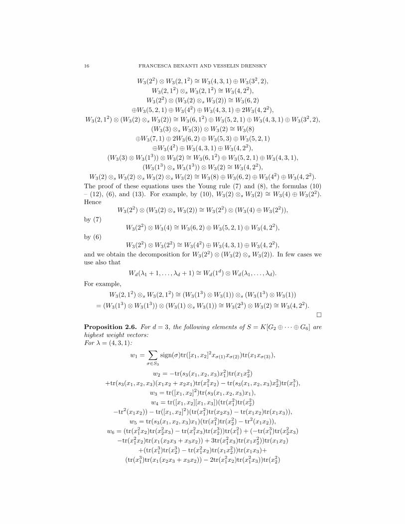
Proposition 2.5. For d = 3, the homogeneous component (ω2(S))(8) of degree 8 of

the square ω2(S) of the augmentation ideal of the symmetric algebra of G2⊕· · ·⊕G6

decomposes as

(ω2(S))(8) = 2W3(8) ⊕ W3(7, 1) ⊕ 4W3(6, 2) ⊕ 3W3(6, 12)

⊕2W3(5, 3) ⊕ 6W3(5, 2, 1) ⊕ 4W3(42) ⊕ 7W3(4, 3, 1)⊕ 9W3(4, 22) ⊕ 4W3(3

2, 2).

Proof. The considerations are similar to those in the proof of Proposition 2.2 andinvolves the equtions

W3(32) ⊗ W3(2) ∼= W3(5, 3) ⊕ W3(4, 3, 1)⊕ W3(3

2, 2),

W3(3, 12) ⊗ W3(3) ∼= W3(6, 12) ⊕ W3(5, 2, 1)⊕ W3(4, 3, 1),

W3(3, 12) ⊗ W3(13) ∼= W3(4, 22),

W3(22, 1) ⊗ W3(3) ∼= W3(5, 2, 1)⊕ W3(4, 22),

W3(22, 1) ⊗ W3(1

3) ∼= W3(32, 2),

W3(22) ⊗s W3(2

2) ∼= W3(42) ⊕ W3(4, 22),


W3(22) ⊗ W3(2, 12) ∼= W3(4, 3, 1)⊕ W3(3

2, 2),

W3(2, 12) ⊗s W3(2, 12) ∼= W3(4, 22),

W3(22) ⊗ (W3(2) ⊗s W3(2)) ∼= W3(6, 2)

⊕W3(5, 2, 1)⊕ W3(42) ⊕ W3(4, 3, 1) ⊕ 2W3(4, 22),

W3(2, 12) ⊗ (W3(2) ⊗s W3(2)) ∼= W3(6, 12) ⊕ W3(5, 2, 1)⊕ W3(4, 3, 1)⊕ W3(32, 2),

(W3(3) ⊗s W3(3)) ⊗ W3(2) ∼= W3(8)

⊕W3(7, 1) ⊕ 2W3(6, 2) ⊕ W3(5, 3) ⊕ W3(5, 2, 1)

⊕W3(42) ⊕ W3(4, 3, 1)⊕ W3(4, 22),

(W3(3) ⊗ W3(13)) ⊗ W3(2) ∼= W3(6, 12) ⊕ W3(5, 2, 1)⊕ W3(4, 3, 1),

(W3(13) ⊗s W3(1

3)) ⊗ W3(2) ∼= W3(4, 22),

W3(2) ⊗s W3(2) ⊗s W3(2) ⊗s W3(2) ∼= W3(8) ⊕ W3(6, 2) ⊕ W3(42) ⊕ W3(4, 22).

The proof of these equations uses the Young rule (7) and (8), the formulas (10)– (12), (6), and (13). For example, by (10), W3(2) ⊗s W3(2) ∼= W3(4) ⊕ W3(2

2).Hence

W3(22) ⊗ (W3(2) ⊗s W3(2)) ∼= W3(2

2) ⊗ (W3(4) ⊕ W3(22)),

by (7)W3(2

2) ⊗ W3(4) ∼= W3(6, 2) ⊕ W3(5, 2, 1)⊕ W3(4, 22),

by (6)W3(2

2) ⊗ W3(22) ∼= W3(4

2) ⊕ W3(4, 3, 1)⊕ W3(4, 22),

and we obtain the decomposition for W3(22) ⊗ (W3(2) ⊗s W3(2)). In few cases we

use also that

Wd(λ1 + 1, . . . , λd + 1) ∼= Wd(1d) ⊗ Wd(λ1, . . . , λd).

For example,

W3(2, 12) ⊗s W3(2, 12) ∼= (W3(13) ⊗ W3(1)) ⊗s (W3(1

3) ⊗ W3(1))

= (W3(13) ⊗ W3(1

3)) ⊗ (W3(1) ⊗s W3(1)) ∼= W3(23) ⊗ W3(2) ∼= W3(4, 22).

�

Proposition 2.6. For d = 3, the following elements of S = K[G2 ⊕ · · · ⊕ G6] are

highest weight vectors:

For λ = (4, 3, 1):

w1 =∑

σ∈S3

sign(σ)tr([x1, x2]2xσ(1)xσ(2))tr(x1xσ(3)),

w2 = −tr(s3(x1, x2, x3)x21)tr(x1x

22)

+tr(s3(x1, x2, x3)(x1x2 + x2x1)tr(x21x2) − tr(s3(x1, x2, x3)x

22)tr(x

31),

w3 = tr([x1, x2]2)tr(s3(x1, x2, x3)x1),

w4 = tr([x1, x2][x1, x3])(tr(x21)tr(x

22)

−tr2(x1x2)) − tr([x1, x2]2)(tr(x2

1)tr(x2x3) − tr(x1x2)tr(x1x3)),

w5 = tr(s3(x1, x2, x3)x1)(tr(x21)tr(x

22) − tr2(x1x2)),

w6 = (tr(x21x2)tr(x

22x3) − tr(x2

1x3)tr(x32))tr(x

21) + (−tr(x3

1)tr(x22x3)

−tr(x21x2)tr(x1(x2x3 + x3x2)) + 3tr(x2

1x3)tr(x1x22))tr(x1x2)

+(tr(x31)tr(x

32) − tr(x2

1x2)tr(x1x22))tr(x1x3)+

(tr(x31)tr(x1(x2x3 + x3x2)) − 2tr(x2

1x2)tr(x21x3))tr(x

22)


+(−2tr(x31)tr(x1x

22) + 2tr2(x2

1x2))tr(x2x3),

w7 = tr(s3(x1, x2, x3))(tr(x31)tr(x

22) − 2tr(x2

1x2)tr(x1x2) + tr(x1x22)tr(x

21)).

For λ = (4, 22):

w1 = tr(s3(x1, x2, x3)x21)tr(s3(x1, x2, x3)),

w2 =∑

σ∈S3

sign(σ)tr(s3(x1, x2, x3)xσ(1)xσ(1))tr(x21xσ(3)),

w3 = tr([x1, x2]2)tr([x1, x3]

2) − tr2([x1, x2][x1, x3]),

w4 = tr2(s3(x1, x2, x3)x1),

w5 = tr([x2, x3]2)tr2(x2

1) − 2tr([x1, x3][x2, x3])tr(x21)tr(x1x2)

+2tr([x1, x2][x2, x3])tr(x21)tr(x1x3) + tr([x1, x3]

2)tr2(x1x2)

−2tr([x1, x2][x1, x3])tr(x1x2)tr(x1x3) + tr([x1, x2]2)tr2(x1x3),

w6 = tr([x1, x3]2)(tr(x2

1)tr(x22) − tr2(x1x2))

−2tr([x1, x2][x1, x3]) ∗ (tr(x21)tr(x2x3) − tr(x1x2)tr(x1x3))

+tr([x1, x2]2)(tr(x2

1)tr(x23) − tr2(x1x3)),

w7 = (−4tr(x1x22)tr(x1x

23) + tr2(x1(x2x3 + x3x2)))tr(x

21)

+4(2tr(x21x2)tr(x1x

23) − tr(x2

1x3)tr(x1(x2x3 + x3x2)))tr(x1x2)

+4(2tr(x21x3)tr(x1x

22) − tr(x2

1x2)tr(x1(x2x3 + x3x2)))tr(x1x3)

+4(−tr(x31)tr(x1x

23) + tr2(x2

1x3))tr(x22)

+4(tr(x31)tr(x1(x2x3 + x3x2)) − 2tr(x2

1x2)tr(x21x3))tr(x2x3)

+4(tr(x31)tr(x1x

22) + tr2(x2

1x2))tr(x23),

w8 = tr2(s3(x1, x2, x3))tr(x21),

w9 = (tr(x21)(tr(x

22)tr(x

23) − tr2(x2x3))

−tr2(x1x2)tr(x23) + 2tr(x1x2)tr(x1x3)tr(x2x3) − tr2(x1x3)tr(x

22))tr(x

21).

For λ = (32, 2):

w1 = −tr([x2, x3]2[x1, x2])tr(x

21)

+tr([x1, x2]([x1, x3][x2, x3] + [x2, x3][x1, x3]))tr(x1x2)

−2tr([x1, x2]2[x2, x3])tr(x1x3) − tr([x1, x3]

2[x1, x2])tr(x22)

+2tr([x1, x2]2[x1, x3])tr(x2x3) − tr([x1, x2]

3)tr(x23),

w2 = tr(s3(x1, x2, x3)[x1, x2])tr(s3(x1, x2, x3)),

w3 = tr(s3(x1, x2, x3)x1)tr([x1, x2][x2, x3]) − tr(s3(x1, x2, x3)x2)tr([x1, x2][x1, x3])

+tr(s3(x1, x2, x3)x3)tr([x1, x2]2),

w4 = tr(s3(x1, x2, x3)x1)(tr(x1x2)tr(x2x3) − tr(x1x3)tr(x22))

+tr(s3(x1, x2, x3)x2)(−tr(x21)tr(x2x3) + tr(x1x2)tr(x1x3))

+tr(s3(x1, x2, x3)x3)(tr(x21)tr(x

22) − tr2(x1x2)).

In each of the cases, every highest weight vector w ∈ W3(λ) ⊂ ω2(S) is equal to a

linear combination of wi.


Proof. The considerations use the decomposition of (ω2(S))(8) given in Proposition2.5. The highest weight vectors have been found as those in Propositions 2.3 and2.4. Of course, if we already know the explicit form of the (candidates for) highestweight vectors wi, we can check that they are linearly independent in ω2(S) andsatisfy the requirements of Lemma 1.1. Since for each λ the number of the highestweight vectors wi coincides with the multiplicity of W3(λ) ⊂ ω2(S) from Proposition2.5, we conclude that every highest weight vector w ∈ W3(λ) ⊂ ω2(S) is equal to alinear combination of wi. �

Finally, we shall calculate the Hilbert series of the kernel of the natural homo-morphism S → C0 for d = 3.

Lemma 2.7. Let d = 3 and let J be the kernel of the natural homomorphism

S → C0. Let the Hilbert series of J be

H(J, t1, t2, t3) =∑

k≥0

hk(t1, t2, t3),

where hk is the homogeneous component of degree k of H(J, t1, t2, t3). Then hk = 0for k ≤ 6,

h7 = S(3,22)(t1, t2, t3),

h8 = S(4,3,1)(t1, t2, t3) + 2S(4,22)(t1, t2, t3) + S(32,2)(t1, t2, t3).

Proof. Clearly, the Hilbert series of the kernel J is equal to the difference of theHilbert series of S and C0. For d = 3 we have that

G2 ⊕ · · · ⊕ G6 = W (2) ⊕ W (3) ⊕ W (13)

⊕W (22) ⊕ W (2, 12) ⊕ W (3, 12) ⊕ W (22, 1) ⊕ W (32)

and its Hilbert series is

H(G2 ⊕ · · · ⊕ G6, t1, t2, t3) =∑

ak1k2k3tk1

1 tk2

2 tk3

3

= S(2) + S(3) + S(13) + S(22) + S(2,12) + S(3,12) + S(22,1) + S(32).

The Hilbert series of the symmetric algebra is

H(S, t1, t2, t3) =∏ 1

(1 − tk1

1 tk2

2 tk3

3 )ak1k2k3

.

Now the result follows by evaluation of the coefficients ak1k2k3and expanding the

first several homogeneous components of the difference of the Hilbert series of Sand of the Hilbert series of C0, which is given in (14). �

Corollary 2.8. For d = 3, the algebra C0 has a minimal system of defining re-

lations with the property that the relations of degree 7 and 8 form GL3-modules

isomorphic, respectively, to W3(3, 22) and W3(4, 3, 1) + 2W3(4, 22) + W3(32, 2).

Proof. If J is the kernel of the natural homomorphism S → C0, then a minimalhomogeneous system of generators of J is obtained as a factor space of J moduloJω(S). Since ω(S) contains no homogeneous elements of degree 1, we obtain thatthe multihomogeneous components of total degree 7 and 8 of J and J/Jω(S) areof the same dimension. Hence J (7) and J (8) are isomorphic as GL3-modules to(J/Jω(S))(7) and (J/Jω(S))(8), respectively, and the conclusion follows from theexpressions of h7 and h8 given in Lemma 2.7. �


3. Main results

Now we present the explicit defining relations of degree 7 of the algebra C3d

for any d ≥ 3 and of degree 8 for the algebra C33, with respect to the generatorsof Abeasis and Pittaluga [1]. As we already mentioned, by (1) it is sufficient togive the defining relations of the algebra C0 generated by traces tr(xi1 · · ·xik

) ofproducts of the traceless matrices xi. As in the previous sections, we denote by Sthe symmetric algebra of the GLd-module G2 ⊕ · · · ⊕ G6 of generators of C0 andcall defining relations of C0 the expressions f = 0, where f is an element of thekernel J of the natural homomorphisms S → C0.

Theorem 3.1. Let d ≥ 3. The algebra C0 does not have any defining relations

of degree ≤ 6. The GLd-module structure of the homogeneous defining relations of

degree 7 of C0, i.e., of the component J (7) in S is

J (7) = Wd(4, 13) ⊕ Wd(3, 22) ⊕ Wd(3, 2, 12) ⊕ Wd(23, 1) ⊕ Wd(2

2, 13) ⊕ Wd(2, 15).

In the notation of Proposition 2.4, the defining relations of C0 which are highest

weight vectors are:

For λ = (4, 13):

(33) 12w1 − 15w2 − 20w3 = 0;

For λ = (3, 22):2w1 − w2 + 2w3 = 0.

For λ = (3, 2, 12):−6w1 + 10w3 − 15w4 + 40w6 = 0.

For λ = (23, 1):12w1 + w2 = 0.

For λ = (22, 13):w2 = 0.

For λ = (2, 15):2w1 − 5w2 = 0.

Proof. In all cases the idea is the same. We already know that there are no relationsof degree ≤ 11 for d = 2 and the only GL3-module of relations is isomorphic toW3(3, 22). Hence, we have to consider the cases in Proposition 2.4 only.

We shall consider in detail the case λ = (4, 13). The possible relations w = 0 arelinear combinations of w1, w2, w3. We assume that

(34) w = ξ1w1 + ξ2w2 + ξ3w3 = 0

and evaluate w on the traceless matrices (2) and (3). The coefficients of the mono-

mials (x(1)11 )4x

(2)12 x

(3)22 x

(4)21 and (x

(1)11 )4x

(2)13 x

(3)32 x

(4)21 are, respectively, 20ξ1 − 8ξ2 + 18ξ3

and 20ξ1 + 12ξ3. Hence the equation (34) implies that

20ξ1 − 8ξ2 + 18ξ3 = 20ξ1 + 12ξ3 = 0.

Up to a multiplicative constant, the only solution of this system is

ξ1 = 12, ξ2 = −15, ξ3 = −20.

Hence, there is only one possible candidate for a defining relation which is a highestweight vector of some Wd(4, 13). We evaluate once again (34) on (2) and (3) forthese values of ξ1, ξ2, ξ3 and obtain that w(x1, x2, x3, x4) = 0. Hence the multiplicityof Wd(4, 13) in J is equal to 1 and the corresponding relation is (33). We want to


mention that the case λ = (3, 14) does not participate in the statement of thetheorem, because the multiplicity of Wd(3, 14) in J is 0. �

Corollary 3.2. The dimension of the defining relations of degree 7 of the algebra

C3d is equal to

r7 = r7(d) =2

7!(d + 1)d(d − 1)(d − 2)(41d3 − 86d2 + 114d− 360).

Proof. Since C3d does not satisfy relations of degree ≤ 6, and the constants are theonly elements of degree 0 in K[tr(X1), . . . , tr(Xd)], the dimension of the relationsof degree 7 of C3d coincides with this dimension in C0. Now the proof is completeusing Theorem 3.1 and the dimension formula (5) for Wd(λ). �

Theorem 3.3. Let d = 3. The GLd-module structure of the homogeneous compo-

nent J (8) of degree 8 in S is

J (8) = W3(4, 3, 1)⊕ 2W3(4, 22) ⊕ W3(3, 22, 2).

In the notation of Proposition 2.6, the defining relations which are highest weight

vectors are:

For λ = (4, 3, 1):

(35) − 6w1 − 18w2 + 3w3 + 3w5 − 8w7 = 0;

For λ = (4, 22): All nontrivial linear combinations of

w1 − 15w2 + 3w3 +21

4w4 −

5

2w5 +

5

2w6 − 3w7 + 2w9 = 0,

−36w2 + 6w3 +27

2w4 − 6w5 + 6w6 − 9w7 + w8 + 6w9 = 0.

For λ = (32, 2):

6w1 + 2w2 − 3w3 − 3w4 = 0.

The number r8 of the defining relations of degree 8 of any homogeneous minimal

system of defining relations of the algebra C33 is equal to 30.

Proof. The decomposition of J (8) is given in Corollary 2.8. The explicit form ofthe highest weight vectors is obtained as in the proof of Theorem 3.1. The numberof defining relations of degree 8 in any homogeneous minimal system of definingrelations for C33 is equal to the dimension of the relations J (8) of C0. For the proofthat r8 = 30 it is sufficient to use the dimension formula (5) for Wd(λ). �

Remark 3.4. Using Lemma 1.2 we can find an explicit basis of the set of definingrelations of degree 7 for C0, d ≥ 3, and of degree 8 for C0, d = 3.

Acknowledgements

This project was started when the second author visited the University of Pa-lermo. He is very grateful for the hospitality and the creative atmosphere duringhis stay there.


References

[1] S. Abeasis, M. Pittaluga, On a minimal set of generators for the invariants of 3×3 matrices,Commun. Algebra 17 (1989), 487-499.

[2] G. Almkvist, W. Dicks, E. Formanek, Hilbert series of fixed free algebras and noncommutative

classical invariant theory, J. Algebra 93 (1985), 189-214.[3] H. Aslaksen, V. Drensky, L. Sadikova, Defining relations of invariants of two 3× 3 matrices,

J. Algebra 298 (2006), 41-57.[4] F. Benanti, V. Drensky, Defining relations of noncommutative trace algebra of two 3 × 3

matrices, Adv. Appl. Math. 37 (2006), No. 2, 162-182.[5] A. Berele, J.R. Stembridge, Denominators for the Poincare series of invariants of small

matrices, Israel J. Math. 114 (1999), 157-175.[6] C. De Concini, D. Eisenbud, C. Procesi, Young diagrams and determinantal varieties, Invent.

Math. 56 (1980), 129-165.[7] D.Z. Djokovic, Poincare series of some pure and mixed trace algebras of two generic matrices,

J. Algebra 309 (2007), No. 1, 654-671.[8] V. Drensky, Free Algebras and PI-Algebras, Springer-Verlag, Singapore, 1999.[9] V. Drensky, Computing with matrix invariants, Math. Balk., New Ser. 21 (2007) (to appear).

[10] V. Drensky, E. Formanek, Polynomial Identity Rings, Advanced Courses in Mathematics,CRM Barcelona, Birkhauser, Basel-Boston, 2004.

[11] V. Drensky, L. Sadikova, Generators of invariants of two 4 × 4 matrices, C.R. Acad. Bulg.Sci. 59 (2006), No. 5, 477-484.

[12] E. Formanek, The Polynomial Identities and Invariants of n × n Matrices, CBMS RegionalConf. Series in Math. 78, Published for the Confer. Board of the Math. Sci. Washington DC,AMS, Providence RI, 1991.

[13] P. Koshlukov, Polynomial identities for a family of simple Jordan algebras, Commun. Algebra16 (1988), 1325-1371.

[14] I.G. Macdonald, Symmetric Functions and Hall Polynomials, Oxford Univ. Press (Claren-

don), Oxford, 1979. Second Edition, 1995.[15] K. Nakamoto, The structure of the invariant ring of two matrices of degree 3, J. Pure Appl.

Algebra 166 (2002), No. 1-2, 125-148.[16] C. Procesi, The invariant theory of n × n matrices, Adv. Math. 19 (1976), 306-381.[17] Yu.P. Razmyslov, Trace identities of full matrix algebras over a field of characteristic zero

(Russian), Izv. Akad. Nauk SSSR, Ser. Mat. 38 (1974), 723-756. Translation: Math. USSR,Izv. 8 (1974), 727-760.

[18] Y. Teranishi, The ring of invariants of matrices, Nagoya Math. J. 104 (1986), 149-161.[19] Y. Teranishi, Linear diophantine equations and invariant theory of matrices, “Commut.

Algebra and Combinatorics (Kyoto, 1985)”, Adv. Stud. Pure Math. 11, North-Holland,Amsterdam-New York, 1987, 259-275.

[20] R.M. Thrall, On symmetrized Kronecker powers and the structure of the free Lie ring, Trans.Amer. Math. Soc. 64 (1942), 371-388.

Dipartimento di Matematica ed Applicazioni, Universita di Palermo, Via Archirafi

34, 90123 Palermo, Italy

E-mail address: [email protected]

Institute of Mathematics and Informatics, Bulgarian Academy of Sciences, 1113

Sofia, Bulgaria

E-mail address: [email protected]

Defining Relations of Minimal Degree of the Trace Algebra of $3 \\times 3$ Matrices

Documents