Brigham Young University Brigham Young University BYU ScholarsArchive BYU ScholarsArchive Theses and Dissertations 2006-11-30 Defining a Model for Tool Consumption Rate on Asphalt Defining a Model for Tool Consumption Rate on Asphalt Reclamation Machines Reclamation Machines Matthew H. Taylor Brigham Young University - Provo Follow this and additional works at: https://scholarsarchive.byu.edu/etd Part of the Mechanical Engineering Commons BYU ScholarsArchive Citation BYU ScholarsArchive Citation Taylor, Matthew H., "Defining a Model for Tool Consumption Rate on Asphalt Reclamation Machines" (2006). Theses and Dissertations. 1293. https://scholarsarchive.byu.edu/etd/1293 This Thesis is brought to you for free and open access by BYU ScholarsArchive. It has been accepted for inclusion in Theses and Dissertations by an authorized administrator of BYU ScholarsArchive. For more information, please contact [email protected], [email protected].

Welcome message from author
This document is posted to help you gain knowledge. Please leave a comment to let me know what you think about it! Share it to your friends and learn new things together.
Transcript

Brigham Young University Brigham Young University
BYU ScholarsArchive BYU ScholarsArchive
Theses and Dissertations
2006-11-30
Defining a Model for Tool Consumption Rate on Asphalt Defining a Model for Tool Consumption Rate on Asphalt
Reclamation Machines Reclamation Machines
Matthew H. Taylor Brigham Young University - Provo
Follow this and additional works at: https://scholarsarchive.byu.edu/etd
Part of the Mechanical Engineering Commons
BYU ScholarsArchive Citation BYU ScholarsArchive Citation Taylor, Matthew H., "Defining a Model for Tool Consumption Rate on Asphalt Reclamation Machines" (2006). Theses and Dissertations. 1293. https://scholarsarchive.byu.edu/etd/1293
This Thesis is brought to you for free and open access by BYU ScholarsArchive. It has been accepted for inclusion in Theses and Dissertations by an authorized administrator of BYU ScholarsArchive. For more information, please contact [email protected], [email protected].

DEVELOPING A MODEL FOR TOOL CONSUMPTION RATE ON
ASPHALT RECLAMATION MACHINES
by
Matthew H. Taylor
A thesis submitted to the faculty of
Brigham Young University
in partial fulfillment of the requirements for the degree of
Master of Science
Department of Mechanical Engineering
Brigham Young University
December 2006

Copyright c© 2006 Matthew H. Taylor
All Rights Reserved

BRIGHAM YOUNG UNIVERSITY
GRADUATE COMMITTEE APPROVAL
of a thesis submitted by
Matthew H. Taylor
This thesis has been read by each member of the following graduate committee andby majority vote has been found to be satisfactory.
Date Kenneth W. Chase, Chair
Date Craig C. Smith
Date Carl D. Sorensen

BRIGHAM YOUNG UNIVERSITY
As chair of the candidate’s graduate committee, I have read the thesis of MatthewH. Taylor in its final form and have found that (1) its format, citations, and bibli-ographical style are consistent and acceptable and fulfill university and departmentstyle requirements; (2) its illustrative materials including figures, tables, and chartsare in place; and (3) the final manuscript is satisfactory to the graduate committeeand is ready for submission to the university library.
Date Kenneth W. ChaseChair, Graduate Committee
Accepted for the Department
Matthew R. JonesGraduate Coordinator
Accepted for the College
Alan R. ParkinsonDean, Ira A. Fulton College ofEngineering and Technology
ABSTRACT
DEVELOPING A MODEL FOR TOOL CONSUMPTION RATE ON
ASPHALT RECLAMATION MACHINES
Matthew H. Taylor
Department of Mechanical Engineering
Master of Science
Asphalt and concrete reclamation machines are used to cut roadways when
a repair is required. The performance of these machines can affect the quality of
road repairs, and cost/profitability for both contractors and governments. We believe
that several performance characteristics in reclamation machines are governed by
the placement and pattern of cutting picks on the cutter head. Previous studies,
focused on mining and excavation applications, have shown strong correlation between
placement and wear.
The following study employs a screening experiment (observational study)
to find significant contributors to tool wear, in applications of asphalt milling or
reclamation. We have found that picks fail by two primary modes: tip breakage,
and body abrasive wear. Results indicate that the circumferential spacing of a bit,
relative to neighboring bits, has the strongest effect on tip breakage. We have also
shown that bit skew angle has a large positive effect on body abrasive wear.

ACKNOWLEDGMENTS
This research was mainly supported by Asphalt Zipper, Inc. Asphalt Zipper
has made significant contributions of both equipment and labor to make the study
possible, and they are gratefully acknowledged for their help.
I would like to acknowledge the long patience of Dr. Ken Chase. He has given
many hours of help, and been a great source of advice and ideas. His impact on me
extends beyond the engineering classroom.
I would also like to acknowledge the help of the Mechanical Engineering Faculty
and staff. They have been an immense help to me and have always been there.
Special thanks to Dr. Carl Sorensen for help and support on many difficult problems
encountered in this work. And, to Dr. Craig Smith for his thoughtful input.
Most of all, I would like to thank my wonderful wife. She is truly a pillar
of strength in my life. I am thankful for her patience with long, odd hours, for her
genuine interest in my research, her playful teasing, and her efforts to motivate me
through to the end.

Contents
Abstract v
Acknowledgments vi
List of Tables xii
List of Figures xv
List of Listings xvii
1 Introduction 1
1.1 Problem Statement and Motivation . . . . . . . . . . . . . . . . . . 1
1.2 Background . . . . . . . . . . . . . . . . . . . . . . . . . . . . . . . 4
1.2.1 Features of Small Reclamation Machines . . . . . . . . . . . 4
1.2.2 Applications . . . . . . . . . . . . . . . . . . . . . . . . . . . 7
1.3 Literature Review . . . . . . . . . . . . . . . . . . . . . . . . . . . . 8
1.3.1 Volume Models . . . . . . . . . . . . . . . . . . . . . . . . . 9
1.3.2 Pick Position and Orientation . . . . . . . . . . . . . . . . . 10
1.3.3 Design Optimization . . . . . . . . . . . . . . . . . . . . . . 13
1.4 Document Overview . . . . . . . . . . . . . . . . . . . . . . . . . . 13
2 Pick Position and Performance 15
2.1 Chevron vs. Scattered Patterns . . . . . . . . . . . . . . . . . . . . 15
2.2 Observations on Vibration . . . . . . . . . . . . . . . . . . . . . . . 17
2.3 Observations on Wear . . . . . . . . . . . . . . . . . . . . . . . . . 18
2.3.1 Pick Failure Mechanisms . . . . . . . . . . . . . . . . . . . . 18
vii

2.3.2 Pick Orientation Effects . . . . . . . . . . . . . . . . . . . . 20
2.3.3 Pick Position Effects . . . . . . . . . . . . . . . . . . . . . . 23
2.4 Effects of Assembly Tolerance . . . . . . . . . . . . . . . . . . . . . 26
3 Modeling Per-Pick Volume Removal 27
3.1 Pick Groove Shape and Material Removal Zone . . . . . . . . . . . 28
3.2 Relative Depth and Cut Cross-Section . . . . . . . . . . . . . . . . 29
3.3 Cross-Sectional Area and Volume . . . . . . . . . . . . . . . . . . . 35
3.4 Verification of Model Results . . . . . . . . . . . . . . . . . . . . . . 35
3.5 Summary of Chapter Variables . . . . . . . . . . . . . . . . . . . . 38
4 Developing an Experiment 39
4.1 Designed Experiment vs. Observational Study . . . . . . . . . . . . 39
4.1.1 Independent Variables and Manufacturing Variation . . . . . 40
4.2 Characterization of Experiment Variables . . . . . . . . . . . . . . . 42
4.2.1 Expanded and Condensed Factor Models . . . . . . . . . . . 45
4.3 Overall Average Pick Consumption Rates . . . . . . . . . . . . . . . 48
4.4 Independent Sampling and Bias . . . . . . . . . . . . . . . . . . . . 48
4.4.1 Cut Overlap Bias . . . . . . . . . . . . . . . . . . . . . . . . 49
5 Conducting the Experiment 51
5.1 Measuring Actual Pick Position and Orientation . . . . . . . . . . . 51
5.2 Data Collection Methods . . . . . . . . . . . . . . . . . . . . . . . . 52
5.3 Controlling Machine Operating Parameters . . . . . . . . . . . . . . 54
6 Analysis of Results 57
6.1 Note on Regression Model Closeness . . . . . . . . . . . . . . . . . 57
6.2 Pick Tip Failure Model . . . . . . . . . . . . . . . . . . . . . . . . . 58
6.2.1 Condensed Factors . . . . . . . . . . . . . . . . . . . . . . . 58
6.2.2 Expanded Factors . . . . . . . . . . . . . . . . . . . . . . . . 59
6.3 Pick Body Failure Model . . . . . . . . . . . . . . . . . . . . . . . . 63
viii

6.3.1 Condensed Factors . . . . . . . . . . . . . . . . . . . . . . . 63
6.3.2 Expanded Factors . . . . . . . . . . . . . . . . . . . . . . . . 66
6.4 Contributors to Tip Radius Variation . . . . . . . . . . . . . . . . . 67
7 Conclusions and Recommendations 71
7.1 Contributions . . . . . . . . . . . . . . . . . . . . . . . . . . . . . . 71
7.2 Conclusions . . . . . . . . . . . . . . . . . . . . . . . . . . . . . . . 72
7.2.1 Multiple Failure Modes . . . . . . . . . . . . . . . . . . . . . 72
7.2.2 Skew Angle Effect . . . . . . . . . . . . . . . . . . . . . . . . 73
7.2.3 Pick Failures, a Poisson Process . . . . . . . . . . . . . . . . 73
7.2.4 Manufacturing Variation . . . . . . . . . . . . . . . . . . . . 73
7.2.5 Observational Studies . . . . . . . . . . . . . . . . . . . . . . 74
7.3 Recommendations . . . . . . . . . . . . . . . . . . . . . . . . . . . . 75
8 Future Work 77
8.1 Dataset Size and Randomization . . . . . . . . . . . . . . . . . . . 77
8.2 Material Flow Between Picks . . . . . . . . . . . . . . . . . . . . . 77
8.3 Predictive Models for Pick Consumption Rate . . . . . . . . . . . . 79
8.4 Design Optimization . . . . . . . . . . . . . . . . . . . . . . . . . . 79
8.5 Variations on Volume Calculation . . . . . . . . . . . . . . . . . . . 81
A Cutter Head Pattern Definitions 83
A.1 Specifications for 30 inch Cutter Head . . . . . . . . . . . . . . . . 83
A.2 Specifications for 48 inch Cutter Head . . . . . . . . . . . . . . . . 85
B Analysis Code Listings 93
B.1 MATLAB/Octave Per-Pick Volume Calculation . . . . . . . . . . . 93
B.2 SolidWorks/VBA Per-Pick Volume Calculation . . . . . . . . . . . . 105
B.3 Poisson Regression and Plotting Code . . . . . . . . . . . . . . . . . 110
B.4 Linear Regression and Plotting Code . . . . . . . . . . . . . . . . . 115
C Regression Procedure 137
ix

C.1 Regression Model Trimming . . . . . . . . . . . . . . . . . . . . . . 138
C.2 Factor Scaling and Similarity . . . . . . . . . . . . . . . . . . . . . 138
C.3 Regression Results . . . . . . . . . . . . . . . . . . . . . . . . . . . 140
C.3.1 Pick Tip Failures (Condensed Factors) . . . . . . . . . . . . 140
C.3.2 Pick Tip Failures (Expanded Factors) . . . . . . . . . . . . . 140
C.3.3 Pick Body Failures (Condensed Factors) . . . . . . . . . . . 142
C.3.4 Pick Body Failures (Expanded Factors) . . . . . . . . . . . . 144
C.4 Model Assumptions, Closeness, and Goodness of Fit . . . . . . . . . 145
C.4.1 Tip Failures, Expanded Factors . . . . . . . . . . . . . . . . 147
C.4.2 Body Failures, Expanded Factors . . . . . . . . . . . . . . . 149
C.4.3 Body Failures, Condensed Factors . . . . . . . . . . . . . . . 151
C.5 Example Backward-Stepwise Regression . . . . . . . . . . . . . . . 153
C.6 Regression Model Variable Values . . . . . . . . . . . . . . . . . . . 155
D Cutter Head Measurement 159
D.1 Variables Summary . . . . . . . . . . . . . . . . . . . . . . . . . . . 167
D.2 Sample Part-Program Report . . . . . . . . . . . . . . . . . . . . . 168
Bibliography 172
x

List of Tables
3.1 Description of labels for cross-section boundary points from Figure 3.4 31
3.2 Coordinates for pick tip locations shown in Figure 3.4 . . . . . . . . 32
3.3 Coordinates for intersection points shown in Figures 3.4 and 3.5 . . 32
4.1 Dependent response – directly observed output variables . . . . . . 42
4.2 Primary independent variables . . . . . . . . . . . . . . . . . . . . . 43
4.3 Global variables, applying to all picks collectively . . . . . . . . . . 43
4.4 Randomly varying experiment variables, adding noise to the results 44
4.5 Key definitions relating to proximate distance . . . . . . . . . . . . 45
4.6 Additional experiment variables potentially correlated to bit failures 47
5.1 Descriptive statistics for bit placement measurements (no edge bits) 51
5.2 Descriptions of Testing Applications . . . . . . . . . . . . . . . . . . 52
5.3 Number of failures by failure mode and application . . . . . . . . . 53
5.4 Descriptive statistics for bit failures on bits considered in the analysis 54
6.1 Tip failure regression results, expanded factors and first order interac-tions . . . . . . . . . . . . . . . . . . . . . . . . . . . . . . . . . . . 59
6.2 Body failure regression results for condensed factors . . . . . . . . . 64
6.3 Body failure regression results for expanded factors . . . . . . . . . 66
A.1 Cutter head lacing pattern specification, 30 inch cutter head . . . . 84
A.2 Cutter head lacing pattern specification, 48 inch . . . . . . . . . . . 85
A.3 Actual lacing pattern measurements, 48 inch . . . . . . . . . . . . . 89
B.1 Function call structure for volume calculation . . . . . . . . . . . . 93
B.2 Function call structure for backward stepwise regression . . . . . . . 115
C.1 Descriptive statistics for un-scaled regression variables . . . . . . . . 139
C.2 Descriptive statistics for scaled regression variables . . . . . . . . . 140
C.3 Regression results for tip failures for expanded factor model . . . . 141
xi

C.4 Regression results for body failures for expanded factor model . . . 142
C.5 Regression results for body failures for expanded factor model . . . 144
C.6 Comparison of coefficients for pick body outlier regression model . . 151
C.7 Unscaled regression model variable values . . . . . . . . . . . . . . . 155
xii

List of Figures
1.1 Asphalt Zipper model AZ-480S mounted on a wheeled loader . . . . 5
1.2 Cutter head used on asphalt reclamation machines . . . . . . . . . . 6
1.3 Flattened pick lacing pattern from the cutter head of an asphalt recla-mation machine . . . . . . . . . . . . . . . . . . . . . . . . . . . . . 6
1.4 Diagram of asphalt reclamation process . . . . . . . . . . . . . . . . 7
1.5 Cutter head used on a continuous mining machine . . . . . . . . . . 9
1.6 The effect of pick spacing on specific energy . . . . . . . . . . . . . 11
1.7 Theory of rock tool interaction effects . . . . . . . . . . . . . . . . . 11
1.8 Conical bit, viewed from cutting direction, showing negative and pos-itive skew angles . . . . . . . . . . . . . . . . . . . . . . . . . . . . 12
2.1 Chevron cutter head pick pattern . . . . . . . . . . . . . . . . . . . 16
2.2 The profile of processed material for an inverted chevron pattern (A)and a scattered chevron pattern (B) . . . . . . . . . . . . . . . . . . 17
2.3 Components of a carbide-tipped attack pick . . . . . . . . . . . . . 18
2.4 Failure paths associated with rock excavation using attack picks[1] . 20
2.5 Definitions of pick orientation angles . . . . . . . . . . . . . . . . . 21
2.6 Flattened pick lacing pattern in a 30 inch wide scattered chevron pat-tern . . . . . . . . . . . . . . . . . . . . . . . . . . . . . . . . . . . 24
2.7 Map of impact locations for each attack pick in a 30 inch wide scatteredchevron pattern . . . . . . . . . . . . . . . . . . . . . . . . . . . . . 25
2.8 Illustration of pattern lacing effect on cutting cross-section for picks 23and 50 of Figure 2.7 . . . . . . . . . . . . . . . . . . . . . . . . . . 25
3.1 Pick body has been found to leave a smooth track along the inside faceof the pick groove . . . . . . . . . . . . . . . . . . . . . . . . . . . . 28
3.2 A simplified pick cutting profile angle of 75 degrees was used to calcu-late per-pick material volume . . . . . . . . . . . . . . . . . . . . . 29
3.3 Section view of pick cut paths in an asphalt slab . . . . . . . . . . . 30
xiii
3.4 A representation of material cross-section for a single pick’s cuttingpath, from Detail B of Figure 3.3 . . . . . . . . . . . . . . . . . . . 31
3.5 Dimensioned sketch (in inches) of a pick’s material cross-section . . 32
3.6 Geometry for effective pick radius Re within a sectioning plane at angleθ and advance distance A . . . . . . . . . . . . . . . . . . . . . . . 34
3.7 Comparison between CAD and MATLAB models of per-pick volumeremoval rate . . . . . . . . . . . . . . . . . . . . . . . . . . . . . . . 36
3.8 Complete CAD model describing cut simulation used in model valida-tion . . . . . . . . . . . . . . . . . . . . . . . . . . . . . . . . . . . 37
4.1 Expected variation in per-pick volume removal, based on cutter headassembly tolerance . . . . . . . . . . . . . . . . . . . . . . . . . . . 41
4.2 Diagram showing definitions and sample values of tip and body sideproximate distance for a selected pick and its axially adjacent neighbors 46
5.1 Image of asphalt in ‘alligatored’ condition . . . . . . . . . . . . . . 53
6.1 Plot of main effects in pick tip failure regression model . . . . . . . 60
6.2 Predicted pick tip failures for extreme combinations of the rT ipPD×aBodyPD interaction effect . . . . . . . . . . . . . . . . . . . . . . 62
6.3 Predicted pick tip failures for extreme combinations of the rT ipPD×aT ipPD interaction effect . . . . . . . . . . . . . . . . . . . . . . . 63
6.4 Plot of main effects on pick body failure (condensed-factor model) . 65
6.5 Predicted pick body failures for extreme combinations of the attack-angle × per-pick-volume interaction effect . . . . . . . . . . . . . . 66
6.6 Plot of main effects on pick body failure (expanded-factor model) . 67
6.7 Plot of bit tip height and bit axial location, versus angular position 68
6.8 Drawing illustrating the definition of the row slope variable . . . . . 69
A.1 Flattened plot of designed bit positions, 30 inch cutter head . . . . 83
A.2 Flattened plot of designed bit positions, 48 inch cutter head . . . . 85
C.1 Plot of main effects on pick tip failure for expanded factor model . . 141
C.2 Plot of interaction effects on pick tip failure for expanded-factor model 142
C.3 Plot of main effects on pick body failure for condensed factor model 143
C.4 Plot of interaction effects on pick body failure, condensed factor model 143
C.5 Plot of main effects on pick body failure for expanded factor model 144
xiv

C.6 Normal probability of residuals for expanded-factor regression on picktip failures . . . . . . . . . . . . . . . . . . . . . . . . . . . . . . . . 147
C.7 Influential observations among pick tip failures . . . . . . . . . . . . 148
C.8 Normal probability of residuals for expanded-factor regression on pickbody failures . . . . . . . . . . . . . . . . . . . . . . . . . . . . . . 149
C.9 Influential observations among pick body failures (expanded factors,including outlier) . . . . . . . . . . . . . . . . . . . . . . . . . . . . 150
C.10 Influential observations among pick body failures (expanded factors) 150
C.11 Normal probability of residuals for condensed-factor regression on pickbody failures . . . . . . . . . . . . . . . . . . . . . . . . . . . . . . 152
C.12 Influential observations among pick body failures (condensed factors) 152
D.1 CMM measurement apparatus and setup . . . . . . . . . . . . . . . 160
D.2 Coordinate system created in the CMM part program . . . . . . . . 161
D.3 Angular construction used to find individual pick tip radius R . . . 163
D.4 Angular construction used to find each pick’s attack angle φa, and clockangle adjustment caa . . . . . . . . . . . . . . . . . . . . . . . . . . 164
D.5 Illustration of variables for transforming measured side angle (sa) intoskew angle φs . . . . . . . . . . . . . . . . . . . . . . . . . . . . . . 165
xv

xvi

Listings
B.1 CutterApp.m . . . . . . . . . . . . . . . . . . . . . . . . . . . . . . 94
B.2 MainVolume.m . . . . . . . . . . . . . . . . . . . . . . . . . . . . . 95
B.3 BitVolume.m . . . . . . . . . . . . . . . . . . . . . . . . . . . . . . 98
B.4 BitArea.m . . . . . . . . . . . . . . . . . . . . . . . . . . . . . . . . 99
B.5 Dominance.m . . . . . . . . . . . . . . . . . . . . . . . . . . . . . . 103
B.6 SectPt.m . . . . . . . . . . . . . . . . . . . . . . . . . . . . . . . . . 104
B.7 sw automation.bas . . . . . . . . . . . . . . . . . . . . . . . . . . . 105
B.8 poisson regress body short sample.R . . . . . . . . . . . . . . . . . 110
B.9 WearAnalysis.m . . . . . . . . . . . . . . . . . . . . . . . . . . . . . 116
B.10 FactGen.m . . . . . . . . . . . . . . . . . . . . . . . . . . . . . . . . 119
B.11 EdgeTrim.m . . . . . . . . . . . . . . . . . . . . . . . . . . . . . . . 126
B.12 BackStepRegres.m . . . . . . . . . . . . . . . . . . . . . . . . . . . 127
B.13 LatexTabMed.m . . . . . . . . . . . . . . . . . . . . . . . . . . . . . 130
B.14 PlotData.m . . . . . . . . . . . . . . . . . . . . . . . . . . . . . . . 132
B.15 PlotInteract.m . . . . . . . . . . . . . . . . . . . . . . . . . . . . . . 134
xvii

xviii

Chapter 1
Introduction
1.1 Problem Statement and Motivation
Asphalt and concrete reclamation machines are used to cut roadways when
a repair is required. The performance of these machines can affect the quality of
road repairs, and cost/profitability for both contractors and governments. We believe
that several performance characteristics in reclamation machines are governed by the
placement and pattern of cutting picks on the cutter head. Following is a list of
important performance measures for reclamation machines.
• Amplitude and frequency of vibration
• Magnitude of dynamic loading on pick, drivetrain, and frame components
• Pick consumption rate
• Torque loading on drivetrain components
• Production rate (power consumption)
• Aggregate size of processed material
• Surface roughness of asphalt after milling
• Profile of reclaimed material after trenching or milling (where material is left in
the trench)
Our specific interest for this study is the pick consumption rate. The cost of
replacement picks, relative to other operating costs, can be quite high. We are aware
1
of a case in which a contractor’s cost for replacement picks turned out higher than his
bid price on the entire road repair project. The rate of pick consumption is difficult
to predict in practice. In normal use, the operator of a small asphalt reclamation
machine is required to stop frequently and inspect each pick.
Studies attempting to define comprehensive models for pick consumption rate
have been conducted, for mining and trenching applications, with limited success.
Other studies in these areas, focusing on the relative pick consumption rate among
picks in a given machine, have been more successful. Although there has been signif-
icant related work in the areas of mining, drilling, and trenching, there is still a lack
of knowledge specific to applications in asphalt.
Based on field observations, we have found that particular pick locations have
higher pick consumption rates than other locations on a given cutter head. This
research focuses on defining a model that will allow us to predict relative pick con-
sumption rate. The objective is to identify and characterize design and operational
parameters of asphalt reclamation machines that can be modified to make the pick
consumption rate more uniform between locations on a cutter head. Any changes
made to machine parameters, in an effort to improve pick consumption rate, are con-
strained by the other performance characteristics listed above. Following is a complete
list of factors believed to affect pick wear.
• Operational parameters
– Cutter head rotational speed
– Machine advance rate (or feed rate)
– Machine cutting depth
• Material flow
– Volume of reworked material
– Clearance for material flow between picks
– Pick tip height above cutter head skin (or cutter drum)
2

• Asphalt properties
– Aggregate size
– Matrix adhesive strength
– Asphalt temperature
– Asphalt and base material moisture content
• Pick position and orientation
– Skew angle
– Attack angle
– Pick tip radius from cutter axis of rotation
– Pattern of placement, relative to adjacent picks (or lacing pattern)
• Pick manufacturing characteristics
– Material strength
– Pick component bond strength
– Dimensional variation
• Pick design characteristics
– Tip diameter
– Cone angle
– Carbide profile
Pick positioning, or lacing pattern design, has been a strong area of focus for
improving cutter head performance. However, previous efforts have taken a casual
approach to controlling uniformity of wear. Ultimately, we would like to develop a set
of design tools capable of optimizing cutter head performance along the performance
measures listed above. The present study aims to lay the ground work for methods
of explicitly controlling pick wear. Particularly, we have developed a method for
3

measuring the volume removed by each pick, and have attempted to relate pick volume
to wear performance.
Dimensional tolerances in manufacturing are another obvious source of non-
uniform wear. Without the benefit of a model relating tolerances to pick wear, ap-
propriate tolerances are difficult to obtain. Since manufacturing methods and costs
are closely tied to manufacturing tolerances, identifying appropriate tolerances can
have a large effect on profitability.
The specific purpose of this study was to identify the primary contributing
factors to uneven bit wear, and rank them by size of effect. This information will
allow manufactures to make a focused improvement effort on production processes
and design of asphalt reclamation cutter heads.
By making the pick consumption rate more uniform, the overall average pick
consumption rate will decrease moderately. Additionally, with a uniform consumption
rate, the machine operator will be required to make fewer inspections, which will
significantly improve productivity.
1.2 Background
1.2.1 Features of Small Reclamation Machines
The small reclamation machines, on which this study will focus, have several
noteworthy features. The following list describes some of these distinguishing features.
• Cutter head powered by a dedicated diesel engine
• Cutter head belt driven, with a gear reduction
• Designed to work as an attachment on the bucket of a loader
• Cutter head rotates in a direction such that asphalt is cut in an upward motion
• Forward motion provided by the host vehicle
• Trench dimensions up to 48 inches wide and 12 inches deep
4

Figure 1.1: Asphalt Zipper model AZ-480S mounted on a wheeled loader
The major components of a small reclamation machine include the cutter head,
engine, frame, and drive system. Figure 1.1 shows an Asphalt Zipper model AZ-480S
mounted on a wheeled loader, with the cutter head displayed prominently. The engine
can be seen on top of the frame. A simplified view of the cutter head used on the
AZ-480S is illustrated in Figure 1.2. Figure 1.3 shows a flattened pattern of pick
locations on this same cutter head.
5

Figure 1.2: Cutter head used on asphalt reclamation machines
Figure 1.3: Flattened pick lacing pattern from the cutter head of an asphalt recla-mation machine
6
1.2.2 Applications
There are several applications in which small asphalt reclamation machines
are appropriate. However, the most common uses are in trenching, patching, and full
depth reclamation. Small asphalt reclamation machines are suited to most small to
medium sized road repair jobs. The class of machines that are the focus of this study
are capable of making cuts up to 48 inches wide. These narrow cuts work well for
most utility trenches and patches. Small reclamation machines weigh between 4,000
and 10,000 pounds, and can be towed by a full sized pickup truck. Transportation
of a large milling machine requires special equipment and permits, and can be very
costly.
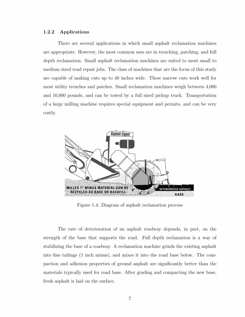
Figure 1.4: Diagram of asphalt reclamation process
The rate of deterioration of an asphalt roadway depends, in part, on the
strength of the base that supports the road. Full depth reclamation is a way of
stabilizing the base of a roadway. A reclamation machine grinds the existing asphalt
into fine tailings (1 inch minus), and mixes it into the road base below. The com-
paction and adhesion properties of ground asphalt are significantly better than the
materials typically used for road base. After grading and compacting the new base,
fresh asphalt is laid on the surface.
7

For roadways that have a sufficiently strong base, repairs of surface deteriora-
tion are performed by milling only a thin layer from the top of the roadway surface.
Small reclamation machines are not well suited to this type of repair work. Rather,
large milling machines are used because of their stability, and ability to make fine
adjustments in depth and angle of cut.
The class of small reclamation machines in this study do not have material
load-out capability, meaning that the material is left in the trench (see Figure 1.4).
Although this can be a problem in a few situations, it is beneficial in most. By leaving
the material in the trench, the cost of adding road base to a road is eliminated. An-
other benefit is the ability of passenger vehicles to drive over the trench immediately
after being cut. This allows a road crew to work on a road, while not disrupting local
traffic.
1.3 Literature Review
Over the last 20 years there has been an increasing amount of effort devoted
to finding optimal parameters for mining equipment. Oil and gas drilling tools have
also received intense study over this period. The published literature includes research
from business, government, and academic sources. Much of this research is focused on
working in hard rock. Published research in the area of asphalt reclamation has been
sparse. However, the equipment and analysis methods used in mining applications
have significant similarities to working in asphalt.
Some of the similarities between mining equipment and asphalt reclamation
equipment are illustrated in Figures 1.2 and 1.5. Figure 1.2 is a drawing of the cutter
head from the reclamation machine shown in Figure 1.1. Figure 1.5 is an image of the
cutter head from a coal shearer. Both pieces of equipment use conical attack picks of
similar size. Also note that the picks are arranged and oriented in a similar pattern.
8

Figure 1.5: Cutter head used on a continuous mining machine
1.3.1 Volume Models
A study of the geometry of oil well drilling heads using diamond-faced cutters
was conducted by Ken Chase [2] in 1978. In conjunction with this study, a computer
program (named Stratapax) was developed, that attempts to optimize dynamic loads
and tool wear characteristics by altering the radial and angular spacing of cutters.
The objective of the optimization was to equalize wear for all of the cutters. Stratapax
calculates for each cutter: the volume of material removed, the cross-sectional area
and radius of gyration of the cut, the torque load, the contact arc, and the wear
surface. The optimal solution criteria of the Stratapax program were chosen based
on expert knowledge rather than analysis of physical data. Dr. Chase believes that
an effort to conduct in situ verification of the results was begun in 1978, but we have
been unable to find any documentation of this effort.
There are noteworthy differences between Chase’s study of drilling heads, and
asphalt reclamation machines. The characteristics of the material being cut are some-
what different. Drilling heads are typically designed to work in hard rock which may
have some similarities to concrete, but which we would expect to behave quite differ-
ently from asphalt. Also, the drilling head studied by Chase makes continuous cuts,
while the asphalt reclamation machine makes interrupted cuts. The effect of this
9

difference is that picks in the asphalt machine experience widely interrupted impact
loads.
An article published in the International Journal of Approximate Reasoning[3]
describes a practical approach for predicting performance of trenching machines.
There appear to be some similarities between trenching in soil and trenching in as-
phalt. However, the failure mechanisms for picks applied in a soil-rock mixture are
much more complex than those of trenching in a homogeneous material, like asphalt.
Parameters of the study included machine advance rate, excavation rate, wear of the
picks, and breakage of the picks, while trench dimensions and total excavated material
volume were fixed. The authors of this study chose to use an approximate reason-
ing method because “Not enough data were available to perform reliable statistical
correlation studies. Therefore, use was made of a Fuzzy Expert System to construct
models that predict production and tool consumption.” The authors report that the
results of their effort were encouraging, but fell short of the stated objective.
1.3.2 Pick Position and Orientation
Research conducted by Sandvik Rock Tools, Inc. relates to the proposed
problem. In a research document titled “Rock Tool Interaction”, Sandvik shows that
the spacing of cutting picks can have a nonlinear effect on the effort required to
remove material. Figure 1.6 shows a plot of specific energy for varying pick spacing.
These results relate to the present study in that changes in specific energy suggest
correlated changes in pick loads, based on pick spacing.
Gary Fuller, the engineer who supervised the Sandvik research, believes that
the effort required to cut asphalt (as opposed to hard rock) is probably linearly related
to pick spacing. The theory used to describe tool interaction in hard rock is illustrated
in Figure 1.7. Mr. Fuller feels that cutting picks will not interact through fracturing
when used in asphalt. He says that Sandvik’s experience has shown a spacing of 5/8
inch to be most effective, but they have not collected supporting data for asphalt.
10

Figure 1.6: The effect of pick spacing on specific energy
Figure 1.7: Theory of rock tool interaction effects
11
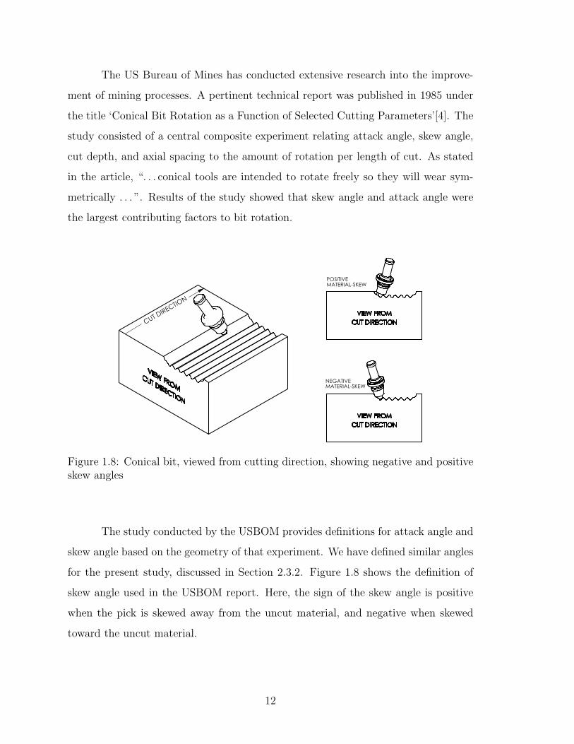
The US Bureau of Mines has conducted extensive research into the improve-
ment of mining processes. A pertinent technical report was published in 1985 under
the title ‘Conical Bit Rotation as a Function of Selected Cutting Parameters’[4]. The
study consisted of a central composite experiment relating attack angle, skew angle,
cut depth, and axial spacing to the amount of rotation per length of cut. As stated
in the article, “. . . conical tools are intended to rotate freely so they will wear sym-
metrically . . . ”. Results of the study showed that skew angle and attack angle were
the largest contributing factors to bit rotation.
�����������
����� ��
�������������
����� ��
�������������
Figure 1.8: Conical bit, viewed from cutting direction, showing negative and positiveskew angles
The study conducted by the USBOM provides definitions for attack angle and
skew angle based on the geometry of that experiment. We have defined similar angles
for the present study, discussed in Section 2.3.2. Figure 1.8 shows the definition of
skew angle used in the USBOM report. Here, the sign of the skew angle is positive
when the pick is skewed away from the uncut material, and negative when skewed
toward the uncut material.
12

1.3.3 Design Optimization
The study of oil well drilling heads, conducted by Chase, applied an optimiza-
tion method used in minimum error linkage design. A detailed description of this
method can be found in another paper by Chase titled ‘Computer-Aided Design of
Precision Control Linkages in the Classroom’[5]. This optimization approach is based
on sensitivity analysis .
Optimization is accomplished for the drilling head, by defining parametric
intervals for bit positions. The magnitude of bit volume error (deviation from the
mean volume for all bits) is used to alter bit positions until volume magnitude is equal
for all bits. Applying sensitivity analysis to this problem proved very computationally
efficient, compared to other optimization techniques.
A study performed by Stephen Rogers and Brian Roberts[1] provides impor-
tant insights into the wear mechanics of cutting picks. They summarize pick wear
mechanics as “complex and almost certainly a composite mechanism”. An important
outcome of this research was a structured view of the possible wear paths for carbide
insert cutting picks. Rogers and Roberts conclude that “the cutting process is an op-
eration where productivity (namely cutting speed and depth), tool wear and product
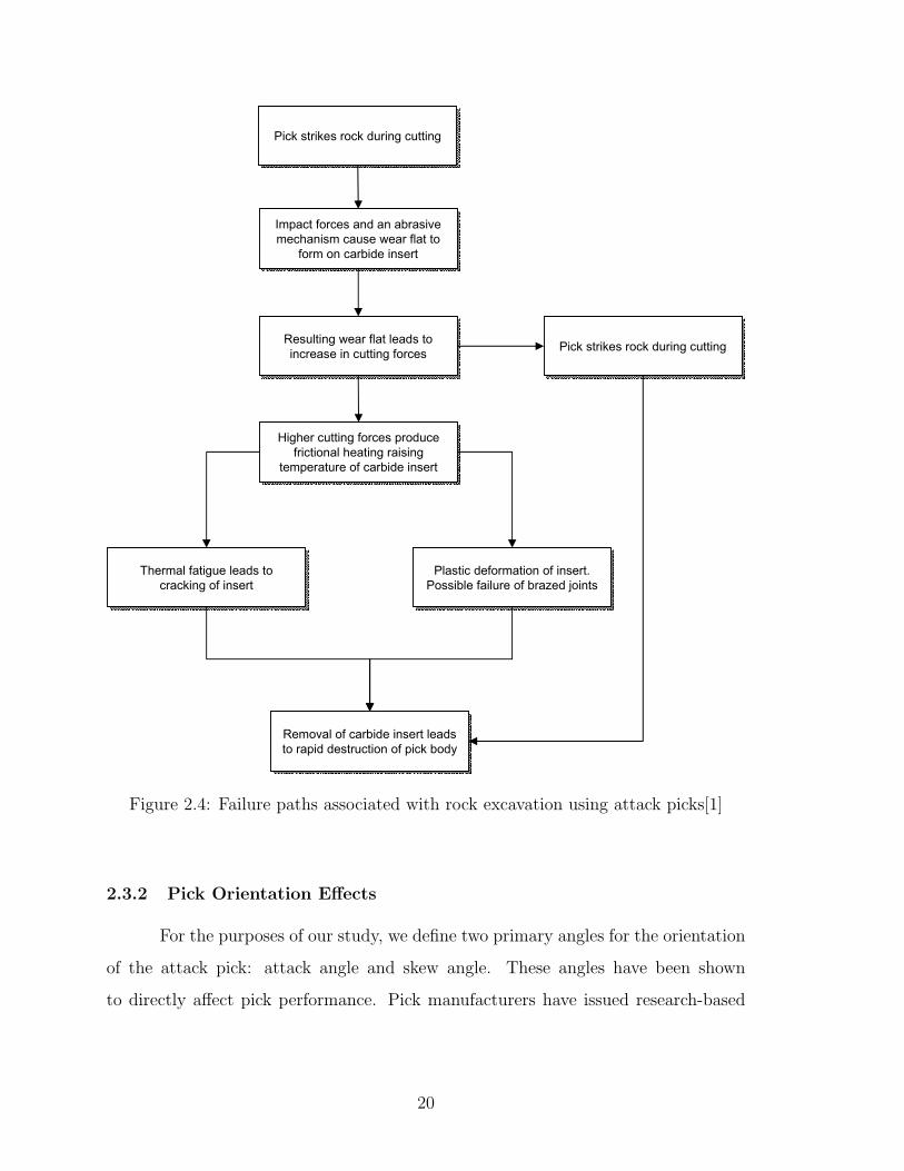
size all need to be optimized”. Figure 2.4 shows some of the results of this study.
1.4 Document Overview
In the following chapters, we develop theories to explain asphalt reclamation
machine performance, and present research to support the theories.
Chapter 2 provides an introduction to pick failure mechanisms, and the sur-
rounding theory. This chapter also covers some of the constraints on cutter head
design.
Chapter 3 details methods for characterizing cutter head design and manu-
facturing in terms of volume removed by each pass of each individual pick. This
characterization helps to simplify our analysis of experimental data.
We provide a detailed description of our experimental design in Chapter 4.
And, Chapter 5 provides details on how the experiment was conducted.
13

Analysis of experimental results is contained in Chapter 6. The bulk of this
chapter is focused on statistical calculations of effects and their significance.
Chapter 8 outlines some possibilities for useful applications of the knowledge
gained in the present study. Also contained in Chapter 8 are some needed extensions
to the present study, and related projects.
The conclusions and recommendations, resulting from this body of work, are
detailed in Chapter 7.
14
Chapter 2
Pick Position and Performance
Most cutter heads do not wear evenly; i.e. certain locations on the cutter head
require more pick replacements than others. In some cases, casual observation will
reveal patterns in individual pick wear, that seem to be related to geometric condi-
tions. We discuss here some of the performance characteristics relating to geometric
parameters of cutter heads. The topics on geometric characteristics of a cutter head
can be categorized as either variational or designed.
2.1 Chevron vs. Scattered Patterns
A common method of laying out a pick pattern is to use a multiple start
chevron pattern. A typical chevron pattern is shown in Figure 2.1. For large milling
machines, this type of pattern has some significant advantages. The main advantage
is that the chevron pattern has the tendency to move material to the center of the
machine. This allows a load-out system to more efficiently move material out of the
cut. Another advantage, is the uniform volume removal rate of the picks. We will
deal with this characteristic of chevron patterns in later sections.
Chevron patterns tend to excite a frequency close to the rate of revolution of
the cutter head. Each time the end of the ‘V’ makes a cutting cycle, most of the
material that has been processed by other picks is reprocessed all at once by a few
picks in the center of the ‘V’. This phenomenon causes a cyclical imbalance in cutter
head loading, which excites a very low resonant frequency mode in the reclamation
machine and host vehicle.
15

�����������
Figure 2.1: Chevron cutter head pick pattern
A significant wear effect can be observed in chevron patterns. Large asphalt
milling machines typically use a load-out system, which requires that processed ma-
terial be pushed toward the center of the cut. Because the material is moved to
the center of the machine, picks located at the center of the cutter head experience
excessive abrasive wear on the body of the picks.
Material processing characteristics of chevron patterns can also be problematic
in some applications. When the end of the ‘V’ engages the material, a few of the
center-most picks have the tendency to act as one large pick, and break out large pieces
of asphalt. In situations where the processed material is to be reused as roadbase,
this is not acceptable. Also, these large pieces of material can cause damage to other
picks, and other machine components.
One solution to these problems is to use an inverted chevron pattern. This
reduces the problems of center pick wear, but has other unwanted effects. Pushing
material to the outer edge of a cut causes the processed material to pile up on the outer
edges. The uneven profile of the processed material is problematic on city streets,
where residents may need to drive over the processed material. Figure 2.2 shows a
sketch of the resulting material profile when using an inverted chevron pattern.
16

�
�
Figure 2.2: The profile of processed material for an inverted chevron pattern (A) anda scattered chevron pattern (B)
Because small reclamation machines generally do not require the load-out ca-
pability provided by a chevron pick lacing pattern, the designs of these machines have
shifted away from chevron patterns. An alternative to chevron patterns is the scat-
tered chevron pattern. Figure 2.6 shows a scattered chevron pattern. This pattern is
based on the chevron, but the chevron lines have been broken into several lines, with
much more distance between picks. This allows processed material to flow between
the picks, rather than being pushed along in front of a row of adjacent picks.
2.2 Observations on Vibration
Small asphalt reclamation machines are plagued by extreme vibration prob-
lems. They have low weight and rigidity relative to the magnitude of impact forces
originating at the cutter head. Typical cutter head patterns have the picks placed
in regular spacing around the circumference of the drum. This arrangement causes
the primary vibration mode to have a very narrow frequency band. In the particular
machine that is the focus of this study, the pick impact frequency has a mean of
approximately 33 cycles per second, with a range of 3 cycles per second.
Our effort to improve pick life is constrained by vibration in the entire system.
In altering the lacing pattern on the cutter head, we must not affect any significant
17
increase in vibration amplitude. Amplitude of vibration may be worsened by moving
to non-uniform circumferential pick spacing. This is because the resonant frequencies
of the reclamation machine and host vehicle will be similar, but not exactly the
same as the pick impact frequency. By randomizing the pick impact frequency, the
bandwidth of the impact frequency will be widened. This widened frequency band has
the effect of moving a portion of the input frequency closer to the resonant frequencies
of the system. Cutter heads are typically designed so that most picks have uniform
axial spacing, thereby condensing vibration excitation into less disruptive regions of
the system’s frequency response spectrum.
2.3 Observations on Wear
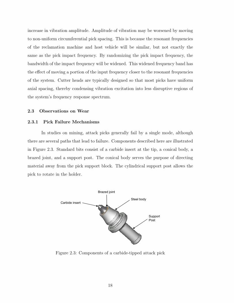
2.3.1 Pick Failure Mechanisms
In studies on mining, attack picks generally fail by a single mode, although
there are several paths that lead to failure. Components described here are illustrated
in Figure 2.3. Standard bits consist of a carbide insert at the tip, a conical body, a
brazed joint, and a support post. The conical body serves the purpose of directing
material away from the pick support block. The cylindrical support post allows the
pick to rotate in the holder.
������������
��� �������
����������
�������
���
Figure 2.3: Components of a carbide-tipped attack pick
18
As each pick passes through the material (asphalt in this case), impact forces
and abrasive mechanisms cause a wear flat to form on the carbide insert. Once this
wear flat forms, the forces required to process material are increased. The increase in
force will, in some cases, immediately remove the carbide insert. When the carbide
insert is removed, the body of the pick is rapidly destroyed.
If the carbide insert is not immediately removed by an increase in cutting
forces, the excess heat generated on the pick introduces two main mechanisms: heat-
ing of the insert leads to thermal fatigue and cracking, and heating of the insert may
cause the brazed joint to fail.
Picks used in asphalt milling machines experience failure paths that are similar
to those of rock excavation picks. However, we have found in our study of asphalt
applications that an additional failure mode is present. Under conditions of high body
wear, a pick will require replacement before the carbide insert is destroyed. In these
cases, although the pick is essentially intact, it must be replaced to prevent abrasive
damage to the pick holder. The exact mechanism by which this happens is at present
unknown, but the result is easily observable.
Figure 2.4, from a study conducted by Stephen Rogers in 1991 [1], shows
typical paths to failure for picks employed in rock excavation.
19
�������������������� ������� ��������������������� ������� �
������������� ��� ���������
���� ��������������������
���� ��������� ���
������������� ��� ���������
���� ��������������������
���� ��������� ���
������ ������������������
� ������ ������ ������
������ ������������������
� ������ ������ ������ �������������������� ������� ��������������������� ������� �
����������� �������������
������ ������� ������� ��
������������������� ���
����������� �������������
������ ������� ������� ��
������������������� ���
���������������������
������ ����� ���
���������������������
������ ����� ������������������ ���� ������
������������������������ ��
��������������� ���� ������
������������������������ ��
���������������� ���������
���������������� �����������
���������������� ���������
���������������� �����������
Figure 2.4: Failure paths associated with rock excavation using attack picks[1]
2.3.2 Pick Orientation Effects
For the purposes of our study, we define two primary angles for the orientation
of the attack pick: attack angle and skew angle. These angles have been shown
to directly affect pick performance. Pick manufacturers have issued research-based
20

recommended values for these angles, to be used in designing cutter heads. These
values vary by application.
Figure 2.5: Definitions of pick orientation angles
Attack angle is defined as the angle from a line tangent to the path of the tip
of a pick, to the axis of the pick body, measured in the plane defined by the circular
path traveled by the pick tip. Skew angle is the angle from the plane defined by the
circular path traveled by the pick tip, to the axis of the pick body, measured in a
plane tangent to the circular path traveled by the pick tip. The sketch of Figure 2.5
illustrates the angle definitions. These angles are described in greater detail in the
referenced literature, and in Appendix D.
So far, we have discussed two different forms of the pick skew angle: that
defined in the USBOM study[4], and the definition of Figure 2.5. In future sections,
we will also make use of the absolute value of the skew angle. It should be noted
21

that while we are using multiple forms of skew angle, all three have identical magni-
tude. For the USBOM study, the sign of the skew angle depends on the surrounding
material. As defined here, the sign of the skew angle is relative to the cutter head.
Other forms of the skew angle used here are the absolute skew angle, and the
standard skew angle. Absolute skew angle is simply the absolute value of the angle.
Standard skew angle is the angle found in cutter head measurements (Appendix D).
For asphalt reclamation machines, the attack angle, as shown in Figure 2.5, is
approximately constrained by the shape of the pick holder (hereafter called a block).
The standard block has constraining features that control its placement on a cutter
head. These features are designed to constrain the attack angle, and are fairly effec-
tive. Pick manufacturers have recommended a skew angle of between 4 and 6 degrees
for the present application. But, skew angle is not constrained by the shape of the
block, and is known to vary significantly in manufacturing.
In general, we have observed that pick orientation has a large effect on wear,
and the skew angle seems to have a larger effect than attack angle. Studies have shown
that, by introducing a small material-negative skew angle, forces are generated that
cause the pick to rotate in its holder. This rotation ensures uniform wear around the
pick. When this rotation is not present, a flat spot is generated on the pick, which
causes rapid failure. The US Bureau of Mines study[4], referenced above, showed that
a skew angle of between 5 and 15 degrees was most effective in inducing rotation in
carbide attack picks. For angles approaching 15 degrees, pick manufacturers find that
significant bending stress is introduced into the pick body. But, no recommendation
is given on the tolerance for skew angle variation.
22

2.3.3 Pick Position Effects
Simple experiments in altering relative pick position suggest that pick posi-
tioning has a large impact on pick wear. We have found that, when inserting a new
pick into a cutter head with worn picks, the new pick will wear rapidly to match the
worn state of the neighboring picks. We hypothesize that this phenomenon can be
quantified in terms of volume removed by the new pick.
When a new pick is inserted between worn picks, its relative height may be
as much as 1/8 of an inch greater than the neighboring picks. This additional height
causes the new pick to remove a greater volume of material in each cutting cycle.
When the new pick has worn to match the neighboring picks, the volumes equalize,
and the wear rate between picks equalizes.
To illustrate the effects of pick position on pick volume removal, we make a
rough estimate of the cross-sectional area of the material removed by each pick. The
volume removed by each pick will be approximately proportional to the estimated
cross-sectional area. This illustration focuses on pick numbers 23 and 50, numbered
in order of impact. While these particular picks represent an extreme case, they serve
well to illustrate the potential effect of pattern layout on volume removal.
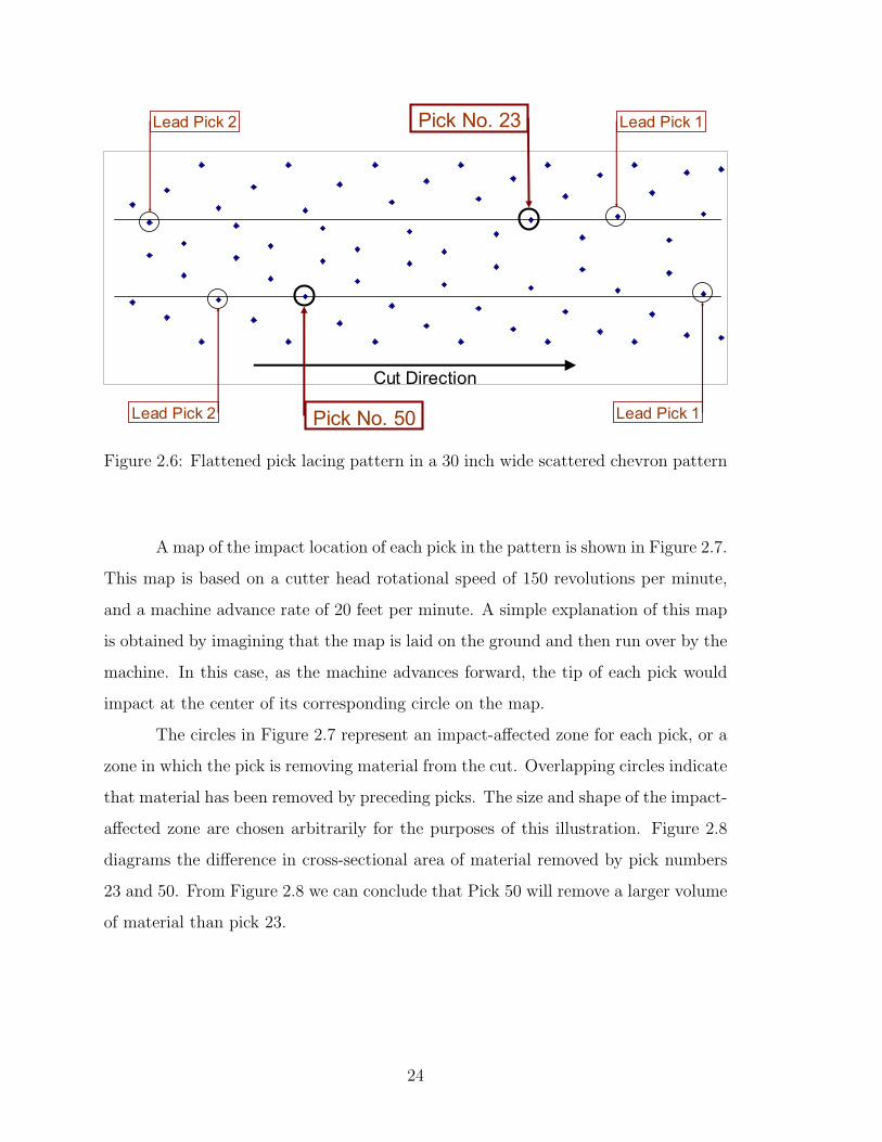
The cutter head pattern used for this illustration is shown in Figure 2.6, with
each dot representing the tip of an attack pick. This pattern is a 30 inch wide scattered
chevron pattern, and is typical of most cutter head patterns. The location of pick
numbers 23 and 50 are also noted in figure 2.6. Horizontal lines have been drawn
through picks 23 and 50 so that the relative locations of neighboring picks can be
easily identified.
Dimensions defining the location of picks in a particular pattern are defined
in terms of axial position referenced from the edge of the cutter head drum, and in
terms of circumferential spacing around the drum based on an arbitrary starting line
(sometimes a seam in the tubing from which the drum is constructed).
23
�����������
�� ��������� ������� ���������
����������� ������� �� �������
Figure 2.6: Flattened pick lacing pattern in a 30 inch wide scattered chevron pattern
A map of the impact location of each pick in the pattern is shown in Figure 2.7.
This map is based on a cutter head rotational speed of 150 revolutions per minute,
and a machine advance rate of 20 feet per minute. A simple explanation of this map
is obtained by imagining that the map is laid on the ground and then run over by the
machine. In this case, as the machine advances forward, the tip of each pick would
impact at the center of its corresponding circle on the map.
The circles in Figure 2.7 represent an impact-affected zone for each pick, or a
zone in which the pick is removing material from the cut. Overlapping circles indicate
that material has been removed by preceding picks. The size and shape of the impact-
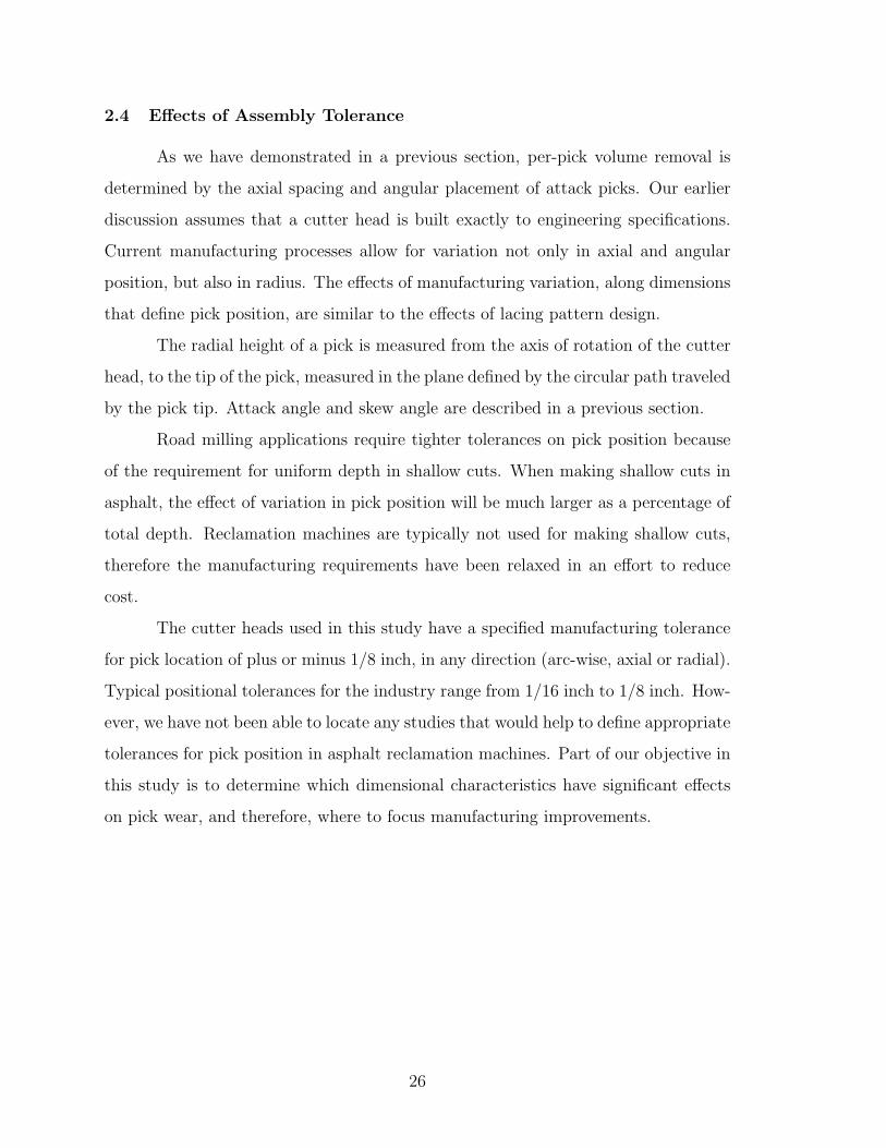
affected zone are chosen arbitrarily for the purposes of this illustration. Figure 2.8
diagrams the difference in cross-sectional area of material removed by pick numbers
23 and 50. From Figure 2.8 we can conclude that Pick 50 will remove a larger volume
of material than pick 23.
24
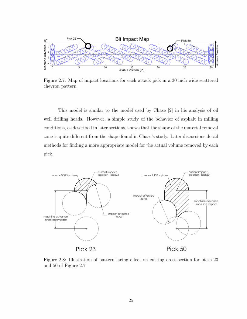
Figure 2.7: Map of impact locations for each attack pick in a 30 inch wide scatteredchevron pattern
This model is similar to the model used by Chase [2] in his analysis of oil
well drilling heads. However, a simple study of the behavior of asphalt in milling
conditions, as described in later sections, shows that the shape of the material removal
zone is quite different from the shape found in Chase’s study. Later discussions detail
methods for finding a more appropriate model for the actual volume removed by each
pick.
����
���������� �������� ����
�������������
�������� ����
�������������
����������
����
������������������
�������������������������
������
������������������
������
�������������������������
Figure 2.8: Illustration of pattern lacing effect on cutting cross-section for picks 23and 50 of Figure 2.7
25
2.4 Effects of Assembly Tolerance
As we have demonstrated in a previous section, per-pick volume removal is
determined by the axial spacing and angular placement of attack picks. Our earlier
discussion assumes that a cutter head is built exactly to engineering specifications.
Current manufacturing processes allow for variation not only in axial and angular
position, but also in radius. The effects of manufacturing variation, along dimensions
that define pick position, are similar to the effects of lacing pattern design.
The radial height of a pick is measured from the axis of rotation of the cutter
head, to the tip of the pick, measured in the plane defined by the circular path traveled
by the pick tip. Attack angle and skew angle are described in a previous section.
Road milling applications require tighter tolerances on pick position because
of the requirement for uniform depth in shallow cuts. When making shallow cuts in
asphalt, the effect of variation in pick position will be much larger as a percentage of
total depth. Reclamation machines are typically not used for making shallow cuts,
therefore the manufacturing requirements have been relaxed in an effort to reduce
cost.
The cutter heads used in this study have a specified manufacturing tolerance
for pick location of plus or minus 1/8 inch, in any direction (arc-wise, axial or radial).
Typical positional tolerances for the industry range from 1/16 inch to 1/8 inch. How-
ever, we have not been able to locate any studies that would help to define appropriate
tolerances for pick position in asphalt reclamation machines. Part of our objective in
this study is to determine which dimensional characteristics have significant effects
on pick wear, and therefore, where to focus manufacturing improvements.
26
Chapter 3
Modeling Per-Pick Volume Removal
In order to investigate the relationship between per-pick-volume and pick wear,
we first needed to define a model relating per-pick-volume to measurable parameters
of a cutter head. In this section, we show that a close approximation of per-pick
volume can be calculated from geometric, and operational parameters. In simple
terms, we calculate the cross-sectional area of a pick’s cut, at several angles through
the cutting cycle, and then integrate those areas to find volume. A summary of this
process follows.
1. Select a primary pick for which to calculate cut-volume, based on impact order
2. Select a subset of picks that interact with the primary pick
3. Divide the primary pick’s cutting path into angularly incremented sectioning
planes
4. For each sectioning plane:
(a) Calculate an effective radius for each interacting pick, lying in the current
sectioning plane
(b) Find intersection points between cutting profiles for the primary pick, its
own previous cutting cycle, and all interacting picks
(c) Calculate the area enclosed by the intersection points
5. Numerically integrate each of the pick’s cutting section area along its cutting
path
27

3.1 Pick Groove Shape and Material Removal Zone
By studying the shape of the grooves formed by picks as they pass through
asphalt, we have developed a model for cut profile. Figure 3.1 shows an area where
a reclamation machine began a cut in asphalt. The feature noted in this image is
a smooth track caused by the body of a pick contacting unprocessed material. The
hardened steel body of the pick continues to make occasional contact with the solid
portions of asphalt throughout the picks effective life. The observation of pick body
contact suggests that asphalt, not in the direct path of the pick (material between
picks), remains intact after a pick has made a near-by pass.
Figure 3.1: Pick body has been found to leave a smooth track along the inside faceof the pick groove
Based on the above observations, we have chosen to use a “V” shaped cutting
profile, at an angle of 75 degrees. In order to verify the geometry of the material
removal zone, we collected a sample of asphalt that had been cut by a single pick.
28

Figure 3.2 shows a cut-away view of the asphalt sample. A true scale sketch of a pick
has been superimposed on the image. A 75 degree “V” has been added to the sketch
to represent the approximated cutting profile.
Figure 3.2: A simplified pick cutting profile angle of 75 degrees was used to calculateper-pick material volume
3.2 Relative Depth and Cut Cross-Section
Most of the effort required to find volume is centered in finding the cross-
sectional area along a pick’s cutting path. In Section 2.3.3, we demonstrate the
relationship between pick position geometry, machine forward speed, cutter head
rotational speed, and pick cutting cross-section. For a more complete model, we also
consider the overall cutting depth of the machine.
Cross-sectional area for an individual pick is defined in a series of sectioning
planes, like the plane illustrated in Figures 3.3. Sectioning planes are defined by
the cutter head axis of rotation and the tip of the current pick. We describe a
material cross-section using a set of points lying in the sectioning plane. These points
are coordinates of the intersections between the “V” shaped cutting profile for all
neighboring picks. Coordinates for these intersections are based on the axis of rotation
of the cutter head, and the edge of the cutter head skin, in the directions shown in
29

Figure 3.4. The dimensioned sketch in Figure 3.5 shows a set of intersection points,
relative to the tip of the current pick.
Boundary points for the included figures are described in Table 3.1. As dis-
played in Figure 3.4, Lines BF and FD represent material remaining immediately
prior to the current picks cutting cycle. Lines EA and AG represent the new ma-
terial boundary, after the current pick completes its cutting cycle. The shaded area
represents the cross-section of material removed in this cutting cycle.
Figure 3.3: Section view of pick cut paths in an asphalt slab
30

Figure 3.4: A representation of material cross-section for a single pick’s cutting path,from Detail B of Figure 3.3
Table 3.1: Description of labels for cross-section boundary points from Figure 3.4
Label DescriptionA Tip location for current pickB Tip location for a previous pass of an adjacent pickC Tip location for previous pass of current pickD Tip location for a previous pass of an adjacent pickE Intersection point between cut profile of picks A and BF Intersection point between cut profile of picks B and DG Intersection point between cut profile of picks A and D
31
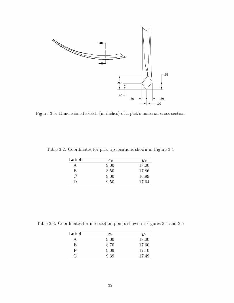
Figure 3.5: Dimensioned sketch (in inches) of a pick’s material cross-section
Table 3.2: Coordinates for pick tip locations shown in Figure 3.4
Label xp yp
A 9.00 18.00B 8.50 17.86C 9.00 16.99D 9.50 17.64
Table 3.3: Coordinates for intersection points shown in Figures 3.4 and 3.5
Label xs ys
A 9.00 18.00E 8.70 17.60F 9.09 17.10G 9.39 17.49
32

The coordinates for the intersection point between any two pick profiles, in
the sectioning plane, are given by Equation 3.1. This equation requires x and y
coordinates for the tip location (xp, yp) of two picks in the sectioning plane. With
the equation in this form, Pick 2 must have x coordinate greater than that of pick 1
(xp2 > xp1). Example pick tip and intersection point coordinates are shown in Tables
3.2 and 3.3 respectively.
xs =(yp2 + m · xp2)− (yp1 −m · xp1)
2m
ys = m · xs + (yp1 −m · xp1); (3.1)
Where:
m = Slope of the line defined by a single side of a pick cutting
profile, lying in the sectioning plane – In this case, m =
tan(90◦ − 75◦
2)
xp = Axial coordinate of a pick tip location, relative to refer-
ence point on edge of cutter head skin: a specific instance
of Da
yp = Radial coordinate of a pick tip location: a specific in-
stance of the variable Re
xs = Axial coordinate of a pick cut profile intersection point,
relative to tip location of current pick
ys = Radial coordinate of a pick cut profile intersection point,
relative to tip location of current pick
Pick tip effective depth within a particular sectioning plane (yp in Table 3.2),
can be found using Equation 3.2. This equation finds an effective radius Re for the
previous pass of a given pick, or the effective depth of its neighboring picks. Variable
definitions for the effective radius equation are listed below, and are illustrated in the
sketch of Figure 3.6.
33

Re = R
sin[π − arcsin
(AR
sin (θ))− θ
]sin (θ)
(3.2)
Where:
Re = Effective pick tip radius for a particular sectioning plane
R = Individual pick tip radius, from rotational axis of cutter
head
A = Machine advance distance between pick impact events
θ = Cutter head rotation angle, measured from negative of
machine advance direction to an individual pick tip
Figure 3.6: Geometry for effective pick radius Re within a sectioning plane at angleθ and advance distance A
34
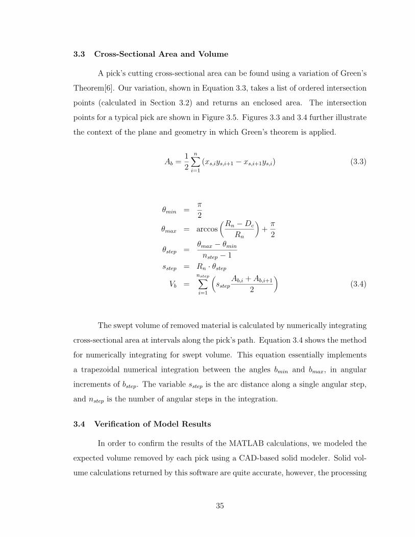
3.3 Cross-Sectional Area and Volume
A pick’s cutting cross-sectional area can be found using a variation of Green’s
Theorem[6]. Our variation, shown in Equation 3.3, takes a list of ordered intersection
points (calculated in Section 3.2) and returns an enclosed area. The intersection
points for a typical pick are shown in Figure 3.5. Figures 3.3 and 3.4 further illustrate
the context of the plane and geometry in which Green’s theorem is applied.
Ab =1
2
n∑i=1
(xs,iys,i+1 − xs,i+1ys,i) (3.3)
θmin =π
2
θmax = arccos(
Rn −Dc
Rn
)+
π
2
θstep =θmax − θmin
nstep − 1
sstep = Rn · θstep
Vb =nstep∑i=1
(sstep
Ab,i + Ab,i+1
2
)(3.4)
The swept volume of removed material is calculated by numerically integrating
cross-sectional area at intervals along the pick’s path. Equation 3.4 shows the method
for numerically integrating for swept volume. This equation essentially implements
a trapezoidal numerical integration between the angles bmin and bmax, in angular
increments of bstep. The variable sstep is the arc distance along a single angular step,
and nstep is the number of angular steps in the integration.
3.4 Verification of Model Results
In order to confirm the results of the MATLAB calculations, we modeled the
expected volume removed by each pick using a CAD-based solid modeler. Solid vol-
ume calculations returned by this software are quite accurate, however, the processing
35

time for these calculations is excessive. Code used to implement volume calculations,
using an Application Program Interface (API) to the CAD package, is included in
Appendix B. The simplified CAD model, used for volume calculations, is also shown
in Appendix B. Figure 3.8 shows a rendering of the complete CAD model.
Per-Pick Volume Model Comparison
0
1
2
3
4
5
6
7
0 5 10 15 20 25 30
Axial Position (in)
Pick Volume (in3)
CAD Model
MATLAB Model
Figure 3.7: Comparison between CAD and MATLAB models of per-pick volumeremoval rate
The comparison illustrated in Figure 3.7 is a plot of the per-pick volume for
each pick, ordered by axial position on the cutter head. Values found from the
MATLAB model lie almost directly over the CAD values, causing the plot to appear
as one line. These results are based on a MATLAB volume calculation using 30
integration steps (nstep = 30). Because processing time with 30 steps is relatively slow,
we used nstep = 10 for tasks requiring iterative model calls (Monte Carlo Simulations).
The processing time is dramatically reduced, with very little loss of accuracy. Overall,
the MATLAB model performs very well.
36
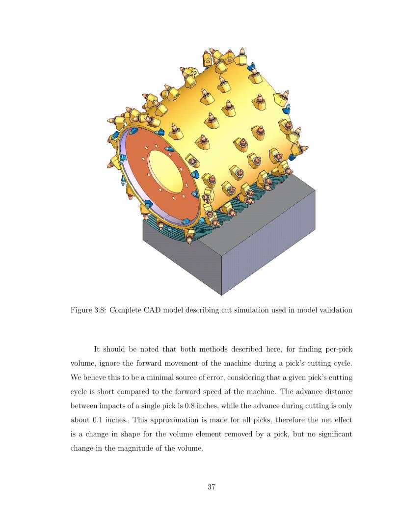
Figure 3.8: Complete CAD model describing cut simulation used in model validation
It should be noted that both methods described here, for finding per-pick
volume, ignore the forward movement of the machine during a pick’s cutting cycle.
We believe this to be a minimal source of error, considering that a given pick’s cutting
cycle is short compared to the forward speed of the machine. The advance distance
between impacts of a single pick is 0.8 inches, while the advance during cutting is only
about 0.1 inches. This approximation is made for all picks, therefore the net effect
is a change in shape for the volume element removed by a pick, but no significant
change in the magnitude of the volume.
37
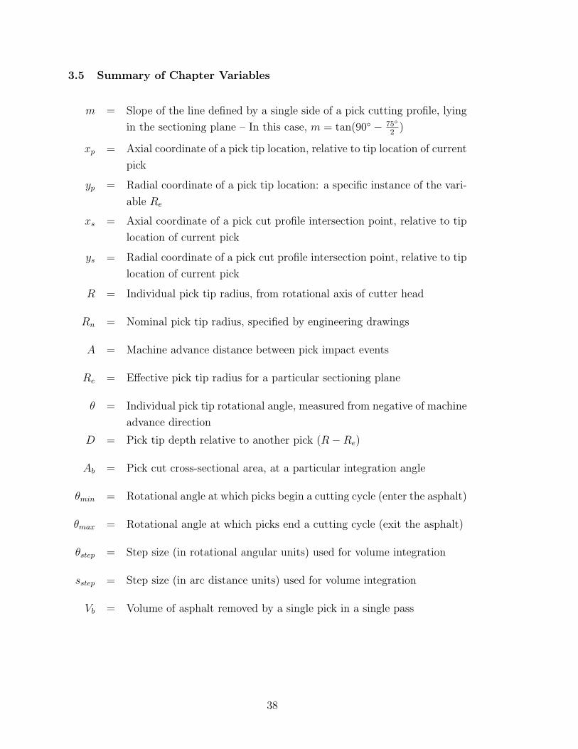
3.5 Summary of Chapter Variables
m = Slope of the line defined by a single side of a pick cutting profile, lying
in the sectioning plane – In this case, m = tan(90◦ − 75◦
2)
xp = Axial coordinate of a pick tip location, relative to tip location of current
pick
yp = Radial coordinate of a pick tip location: a specific instance of the vari-
able Re
xs = Axial coordinate of a pick cut profile intersection point, relative to tip
location of current pick
ys = Radial coordinate of a pick cut profile intersection point, relative to tip
location of current pick
R = Individual pick tip radius, from rotational axis of cutter head
Rn = Nominal pick tip radius, specified by engineering drawings
A = Machine advance distance between pick impact events
Re = Effective pick tip radius for a particular sectioning plane
θ = Individual pick tip rotational angle, measured from negative of machine
advance direction
D = Pick tip depth relative to another pick (R−Re)
Ab = Pick cut cross-sectional area, at a particular integration angle
θmin = Rotational angle at which picks begin a cutting cycle (enter the asphalt)
θmax = Rotational angle at which picks end a cutting cycle (exit the asphalt)
θstep = Step size (in rotational angular units) used for volume integration
sstep = Step size (in arc distance units) used for volume integration
Vb = Volume of asphalt removed by a single pick in a single pass
38

Chapter 4
Developing an Experiment
The primary focus of this experiment is to determine the strength of the rela-
tionship between pick position/orientation, and pick failure rate. In previous sections,
we have defined three main variables that will be our primary experiment factors: ab-
solute skew angle, attack angle, and per-pick volume removal. The response variable
for our experimentation is the pick failure rate.
4.1 Designed Experiment vs. Observational Study
Using a designed experiment requires precise control over the factors of inter-
est, in our case pick position and orientation. This study is motivated by the fact
that these factors are difficult to control. Because of this difficulty, we have chosen
to obtain data under an observational study framework.
There are certain trade-offs when choosing between an observational study and
a designed experiment. Typically, a designed experiment would have to be conducted
in a laboratory in order to explicitly control all of the variables. And, some operating
conditions would be impossible to simulate in the lab.
On the other hand, observational studies have certain difficulties. Measure-
ments in the field are expected to be more difficult, and less accurate. In the present
study, we simply collect observations of performance under conditions of natural vari-
ation in all experiment variables. Under these conditions, it is impossible to detect
the presence of lurking variables from statistical analysis of the results. This means
there is a strong potential for confounded results, or results that cannot be verified
by statistical methods. In order to validate our results, we have shown by expert
39

knowledge of the systems involved, that all potential variables have been sufficiently
accounted for.
Designed experiments are setup in such a way that data are collected at the
boundaries of the model space. Since in an observational study we are unable to
choose factor values, the boundaries are not fully explored. This can lead to mislead-
ing results, as some regions of the predictive model actually use extrapolations of the
data.
The specific objective of the experiment was to relate the pick failure rate to
the volume removal and to the orientation of each pick location. Table 4.2 describes
the three primary explanatory variables that make up our experiment. Section 2.3.2
describes in detail how skew and attack angles affect individual pick wear.
4.1.1 Independent Variables and Manufacturing Variation
The attractiveness of an observational study for this research is derived from
the large manufacturing variation observed in the construction of cutter heads. There
are 96 picks in the main pattern of a 48 inch wide cutter head. We assume that each
pick is defined by a set of independent random variables. This situation provides us
with a large amount of data from a single cutter head.
Using the methods described in Chapter 3, we have calculated expected vari-
ation in the volume of material removed by each pick. These calculations are based
on the dimensional tolerance from engineering assembly drawings. Figure 4.1 shows
nominal volume for each pick location on a particular cutter head. Also shown, are
expected variation found from two different methods of calculation. The Monte Carlo
method is simple to implement, but very resource intensive. The Direct Linearization
Method (DLM) returns accurate results, with very few calculations. A comparison
of the two methods can be found in a study by Gao, Chase, and Magleby[7].
40

Volume Tolerance Analysis
0
1
2
3
4
5
6
7
8
9
0 5 10 15 20 25 30
Axial Position (in)
Volume (in3)
MonteCarlo Tolerance
DLM Tolerance
Nominal Volume
Figure 4.1: Expected variation in per-pick volume removal, based on cutter headassembly tolerance
Both the DLM, and the Monte Carlo method produce a root-sum-squares
(RSS) assembly tolerance for per-pick material volume. The error bars on the nominal
volume represent a plus-or-minus three sigma (3σ) variation in per-pick volume. A
separate plot of the one-sided 3σ variation for each of the analysis methods is also
included in Figure 4.1.
It can be seen from the DLM and Monte Carlo tolerance plots, of Figure
4.1, that there is very close agreement between the two methods. There are three
main issues effecting the accuracy of these methods. First, Monte Carlo accuracy
depends on making a large number of model calls, which can be very time intensive
(we performed only 15,000 iterations). Second, DLM performs a linearization on the
input model, which can introduce errors where tolerances are large relative to nominal
dimensions. Third, the DLM assumes a Normal distribution for both manufacturing
tolerances and volume variation, but non-linearity in manufacturing tolerances can
cause the actual distribution of volume variation to be skewed. The DLM method
has been shown to have accuracy equivalent to a Monte Carlo analysis with 30,000
model calls[7].
41

4.2 Characterization of Experiment Variables
The response variable for our experimentation is the locational pick failure
rate. This rate is defined as the number of picks replaced in a particular location on
an existing cutter head, throughout all testing. Note that we have not defined this
rate in terms of time, but rather in terms of count-per-experiment (see Table 4.1).
Table 4.1: Dependent response – directly observed output variables
Variable Name Factor Description
tipFails Individual pick tip failure count, bycutter head location, for the presentexperiment
bodyFails Individual pick body failure count, bycutter head location, for the presentexperiment
Two main characteristics of the experimental design allow us to ignore time
between failures. First, defining per-pick volume makes each pick location on a cutter
head an independent statistical sample. Second, each pick location will experience
the same amount of run time. Under this scenario, the knowledge gained from the
experiment will only allow us to identify significant factors for predicting failures; we
will not be able to predict time-to-failure for a particular pick location.
The main predictive variables that are the focus of this study are pick absolute
skew angle, attack angle, and per-pick volume removal. These three factors can either
be measured directly, or calculated from direct measurements of a cutter head. The
measurement of the factors of interest is fairly simple, with appropriate equipment
(refer to Section 5.1).
42
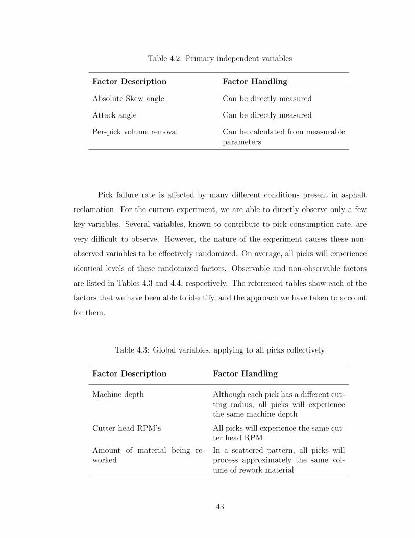
Table 4.2: Primary independent variables
Factor Description Factor Handling
Absolute Skew angle Can be directly measured
Attack angle Can be directly measured
Per-pick volume removal Can be calculated from measurableparameters
Pick failure rate is affected by many different conditions present in asphalt
reclamation. For the current experiment, we are able to directly observe only a few
key variables. Several variables, known to contribute to pick consumption rate, are
very difficult to observe. However, the nature of the experiment causes these non-
observed variables to be effectively randomized. On average, all picks will experience
identical levels of these randomized factors. Observable and non-observable factors
are listed in Tables 4.3 and 4.4, respectively. The referenced tables show each of the
factors that we have been able to identify, and the approach we have taken to account
for them.
Table 4.3: Global variables, applying to all picks collectively
Factor Description Factor Handling
Machine depth Although each pick has a different cut-ting radius, all picks will experiencethe same machine depth
Cutter head RPM’s All picks will experience the same cut-ter head RPM
Amount of material being re-worked
In a scattered pattern, all picks willprocess approximately the same vol-ume of rework material
43
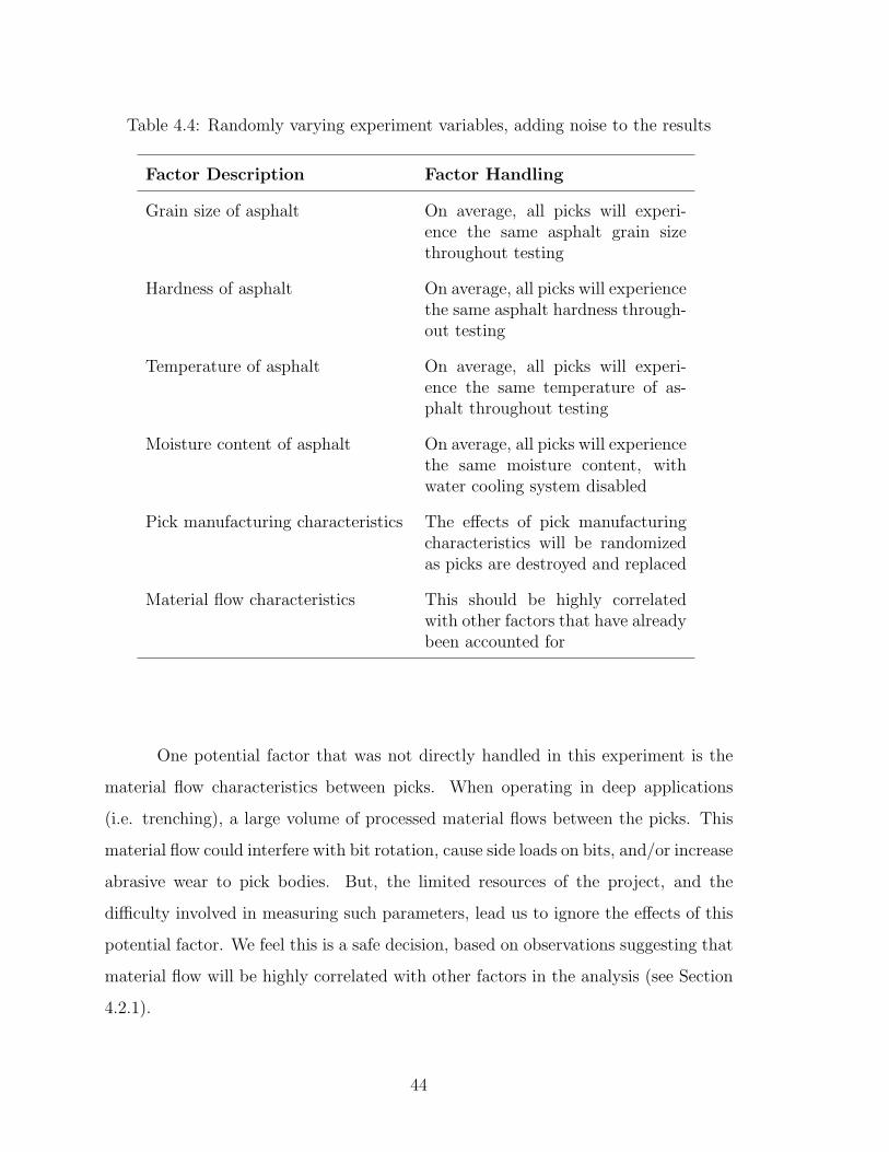
Table 4.4: Randomly varying experiment variables, adding noise to the results
Factor Description Factor Handling
Grain size of asphalt On average, all picks will experi-ence the same asphalt grain sizethroughout testing
Hardness of asphalt On average, all picks will experiencethe same asphalt hardness through-out testing
Temperature of asphalt On average, all picks will experi-ence the same temperature of as-phalt throughout testing
Moisture content of asphalt On average, all picks will experiencethe same moisture content, withwater cooling system disabled
Pick manufacturing characteristics The effects of pick manufacturingcharacteristics will be randomizedas picks are destroyed and replaced
Material flow characteristics This should be highly correlatedwith other factors that have alreadybeen accounted for
One potential factor that was not directly handled in this experiment is the
material flow characteristics between picks. When operating in deep applications
(i.e. trenching), a large volume of processed material flows between the picks. This
material flow could interfere with bit rotation, cause side loads on bits, and/or increase
abrasive wear to pick bodies. But, the limited resources of the project, and the
difficulty involved in measuring such parameters, lead us to ignore the effects of this
potential factor. We feel this is a safe decision, based on observations suggesting that
material flow will be highly correlated with other factors in the analysis (see Section
4.2.1).
44
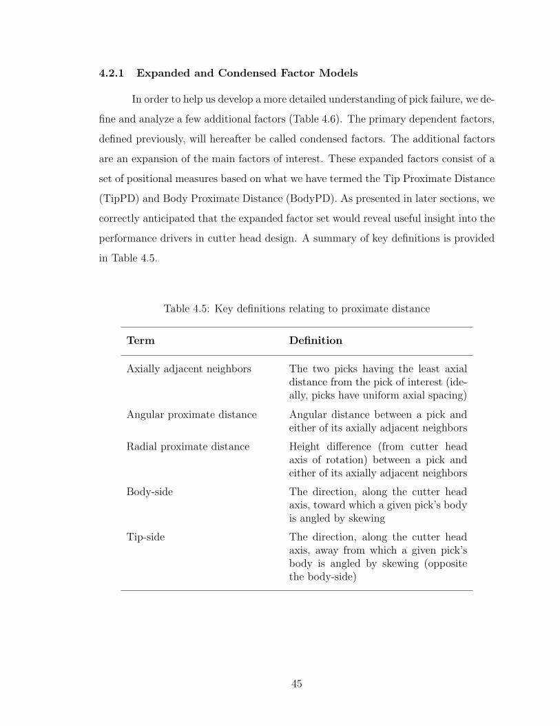
4.2.1 Expanded and Condensed Factor Models
In order to help us develop a more detailed understanding of pick failure, we de-
fine and analyze a few additional factors (Table 4.6). The primary dependent factors,
defined previously, will hereafter be called condensed factors. The additional factors
are an expansion of the main factors of interest. These expanded factors consist of a
set of positional measures based on what we have termed the Tip Proximate Distance
(TipPD) and Body Proximate Distance (BodyPD). As presented in later sections, we
correctly anticipated that the expanded factor set would reveal useful insight into the
performance drivers in cutter head design. A summary of key definitions is provided
in Table 4.5.
Table 4.5: Key definitions relating to proximate distance
Term Definition
Axially adjacent neighbors The two picks having the least axialdistance from the pick of interest (ide-ally, picks have uniform axial spacing)
Angular proximate distance Angular distance between a pick andeither of its axially adjacent neighbors
Radial proximate distance Height difference (from cutter headaxis of rotation) between a pick andeither of its axially adjacent neighbors
Body-side The direction, along the cutter headaxis, toward which a given pick’s bodyis angled by skewing
Tip-side The direction, along the cutter headaxis, away from which a given pick’sbody is angled by skewing (oppositethe body-side)
45

Figure 4.2: Diagram showing definitions and sample values of tip and body sideproximate distance for a selected pick and its axially adjacent neighbors
Tip-side and body-side, for a given pick, are defined by the skew angle for the
pick as shown in Figure 4.2. As labeled in the figure, the body-side of a pick is the
46

direction along the axis of the drum toward which the body of the pick is angled,
by skewing. The Tip PD is the distance from a given pick to the axially adjacent
neighbor on the tip side, along a specified dimension. Tip Radial PD is the radial
distance between a pick and its axially adjacent neighboring picks. Axial PD is the
axial distance between a pick and its axially adjacent neighboring picks.
Angular PD is the angular distance between a pick and either of its axially
adjacent neighboring picks, measured in the forward direction; i.e. angular PD is
measured in the pick’s direction of travel. This is illustrated in Figure 4.2 for the
body-side PD, where angular distance (dimension broken at ‘aBodyPD’) is measured
the long way around the drum.
Using expanded factors allows us to more effectively test the interaction be-
tween per-pick volume and skew angle. The condensed factor set, described in the
preceding section, does not account for the fact that a given pick may cut more as-
phalt on its body side than it does on its tip side. Similarly, a given cutting volume
may have a different effect on the body side than it does on the tip side.
Table 4.6: Additional experiment variables potentially correlated to bit failures
Variable Name Factor Description
xBodyPD Axial body-side proximate distance
xTipPD Axial tip-side proximate distance
rBodyPD Radial body-side proximate distance
rTipPD Radial tip-side proximate distance
aBodyPD Angular body-side proximate distance
aTipPD Angular tip-side proximate distance
47

4.3 Overall Average Pick Consumption Rates
In an effort to approximate the amount of data that would be needed for
significant results, we collected some preliminary data on overall pick consumption
rate per machine. We collected data from information on pick sales and machine
hours. The data were collected from 3 different customers, using information on pick
sales and machine hours. Due in part to a wide variety of applications, the data we
collected had a very large range. The first customer averaged a consumption rate of
30 picks per hour, the second averaged a consumption rate of 1 pick per hour, and
the third averaged 5 picks per hour. By considering the applications in which these
data were collected, we anticipated a pick consumption rate for our experiment of 20
picks per hour. We will show in a later section that this approximation was much
higher than the actual.
4.4 Independent Sampling and Bias
The assumption that each pick location represents an independent observation
is only approximately true. For example, if a particular pick fails, and the machine
continues to operate, the neighboring picks will experience an increased load until
the failed pick is replaced. This situation will cause pick failures in neighboring pick
positions. By stopping the reclamation machine for inspection and data recording at
frequent intervals, the dependency between wear rate of neighboring picks is reduced.
The solution to this dependency problem is to closely monitor the state of each
pick, and replace it as soon as it fails. However, characteristics of asphalt reclamation
make it very difficult to continuously monitor the state of individual picks. As a
result, we are required to collect data at certain intervals in time (i.e. readout data).
Because the precision of our analysis depends on the time resolution of the data
collected, choosing the length of the time interval requires careful consideration.
The ideal interval would approximately match the life of the shortest lived
pick. However, since we have very little predictive capability, we are unable to di-
rectly determine the actual life of any pick. Our approximation of average overall
48

pick consumption rate is useful in determining an initial target for the readout in-
terval, however, the optimum interval is expected to vary by circumstance. In actual
application, we start with an initial target for readout interval, and then adjust that
interval based on observations in that application.
An alternative approach to reducing inter-pick failure dependency is to replace
picks before they completely fail. This could be accomplished by creating a ‘not-go’
gage to be used in determining a uniform level of wear at which a pick is to be
replaced. While this method has attractive statistical attributes, it is difficult to
apply in practice, considering that multiple failure modes have been identified.
4.4.1 Cut Overlap Bias
It was expected that on some jobs, a machine operator would make multiple
adjacent cuts with the reclamation machine. In this case, the machine’s path may
overlap the trench left by a previous path. The result of this situation is that not all
of the picks on the cutter head will be engaging material, which would be a serious
disruption to our experiment. In order to avoid the resulting bias in our data, we
required the machine operator to make several long passes, without significant overlap.
We then discarded data from picks located within a certain distance of the edge of
the cutter head.
49

50

Chapter 5
Conducting the Experiment
5.1 Measuring Actual Pick Position and Orientation
The first task in our experimentation was to make accurate location and orien-
tation measurements for each bit on a particular cutter head. We used a Romer/Cim-
core brand articulated arm CMM (model ‘10 foot Infinite Arm’) to take the measure-
ments. These measurements were performed on empty pick mounting blocks, and
then transformed, based on the shape of the style of pick to be used in our study.
This approach is possible because of the relatively low dimensional variation between
picks. Appendix D details the setup, methods, and results of these measurements.
Based on measurement repetition, we estimate that all measurements are accurate
within ±.015 inches.
Table 5.1: Descriptive statistics for bit placement measurements (no edge bits)
Mean Max Min StDevAxial Spacing 0.5” 0.67” 0.32” 0.08”Tip Radius 17.92” 18.01” 17.84” 0.04”Left Skew -11.5◦ -7.3◦ -18.2◦ 2.3◦
Right Skew 6.0◦ 11.6◦ 1.9◦ 2.1◦
Attack Angle 51.9◦ 53.6◦ 50.2◦ 0.7◦
With precise information on pick location and orientation, we were able to
use the previously discussed computer model to calculate the volume per cutter head
51

revolution removed by each pick, for specified operating parameters. The other factors
of interest, listed in Table 4.2 were also readily available from the transformed CMM
measurements. Descriptive statistics for the bits that were used in the analysis are
shown in Table 5.1.
5.2 Data Collection Methods
Data were collected on various job sites, in various applications. Approximate
times and descriptions of the applications in which we conducted tests are shown in
Table 5.2, comprising a total of 50 hours of operation.
Because of the way asphalt milling attachments are operated, different appli-
cations can affect large changes in some of our factors of interest. Most notable is
the effect of machine forward speed on per-bit-volume. In thin, or soft, material the
machine’s forward speed averaged about 25 feet per minute, whereas in hard or thick
material the machine’s forward speed was between 8 and 10 feet per minute. The
actual average forward speed for the three different material types in our testing were
recorded by the operator, and are shown in Table 5.2.
Table 5.2: Descriptions of Testing Applications
TestingTime
ApplicationDescription
Bit Re-placements
ForwardSpeed
12 hours thin, ‘alligatored’ 27 25 ft/min
35 hours deep, hard 55 10 ft/min
3 hours deep, soft 30 20 ft/min
The first application listed in Table 5.2 is described as ‘alligatored.’ This term
refers to a state of asphalt paving where the material is broken into uniform pieces,
but the material is still in place. An example image of alligatored asphalt is included
in Figure 5.1
52

Figure 5.1: Image of asphalt in ‘alligatored’ condition
Data collected during testing were recorded by the machine operator. The
machine operator reported that in softer materials, some of the bits experienced
a significant amount of body wear. In some cases, the operator was required to
replace these bits before they had completely failed, to avoid damaging the block.
These body-wear-failures represent a separate failure mode of which we were not
previously aware. The number of body and tip failures are compared in Table 5.3.
Total descriptive statistics for the bits considered in our analysis, based on cut overlap,
are presented in Table 5.4.
Table 5.3: Number of failures by failure mode and application
Failure ModeApplications Pick Tip Pick BodyMaterial Type 1 7 20Material Type 2 54 1Material Type 3 0 30
53

Table 5.4: Descriptive statistics for bit failures on bits considered in the analysis
tipFails bodyFailsObservations 90 90Total Failures 55 33Zero Counts 43 64Max Failure Count 2 3Mean Failures 0.61 0.37
5.3 Controlling Machine Operating Parameters
During operation, the operator of the host vehicle (a wheeled loader in this
case) attempts to operate the milling machine forward at a constant cutting torque.
Engine rotational speed is the most convenient indicator of cutting torque. The
operator attempts to hold the milling machine’s engine at a constant rotational speed
(measured in RPM). In our experimentation, the engine speed averaged 2300 RPM.
With a 18:1 gear reduction, this results in a cutter head rotational speed of about
130 RPM.
The host vehicle operator is not able to directly control machine advance rate.
If he pushes too hard with the loader, the milling machine’s engine will stall. By fixing
the depth of cut, and by operating with the milling machine’s engine at a speed for
optimal torque, the machine advance rate can only be observed. Forward speeds for
each testing application are shown in Table 5.2.
Although we intended to operate the machine dry (without the use of water
spray), this was not possible because of restrictions from local health departments.
Operating with a light spray of water prevents the formation of hazardous dust. Our
general observations of the machine’s operation indicated that the light water spray
had no significant effect on performance, or on our data.
In our testing, we found that in full depth reclamation, the cutter head en-
counters a significant amount of moisture in the road base. This makes the proportion
of moisture content coming from the spray system small relative to the total amount
54

of moisture experienced by the bits. We were also careful to check the spray system
at regular intervals to make sure that the spray pattern remained uniform. By taking
these precautions, we have limited the potential for bias in the results of the testing.
55

56
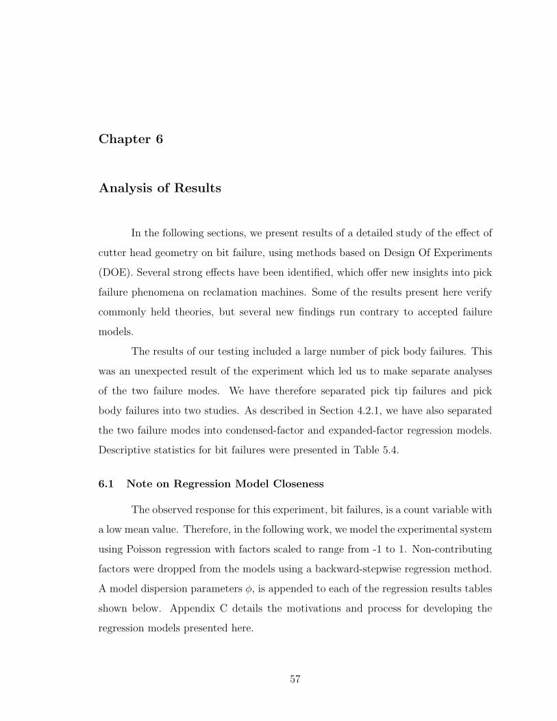
Chapter 6
Analysis of Results
In the following sections, we present results of a detailed study of the effect of
cutter head geometry on bit failure, using methods based on Design Of Experiments
(DOE). Several strong effects have been identified, which offer new insights into pick
failure phenomena on reclamation machines. Some of the results present here verify
commonly held theories, but several new findings run contrary to accepted failure
models.
The results of our testing included a large number of pick body failures. This
was an unexpected result of the experiment which led us to make separate analyses
of the two failure modes. We have therefore separated pick tip failures and pick
body failures into two studies. As described in Section 4.2.1, we have also separated
the two failure modes into condensed-factor and expanded-factor regression models.
Descriptive statistics for bit failures were presented in Table 5.4.
6.1 Note on Regression Model Closeness
The observed response for this experiment, bit failures, is a count variable with
a low mean value. Therefore, in the following work, we model the experimental system
using Poisson regression with factors scaled to range from -1 to 1. Non-contributing
factors were dropped from the models using a backward-stepwise regression method.
A model dispersion parameters φ, is appended to each of the regression results tables
shown below. Appendix C details the motivations and process for developing the
regression models presented here.
57

For the present study (an observational study), the factors being studied have
only natural variation whereas, in a designed experiment, special variation would be
intentionally introduced to the model. For each factor, variation about the mean is
smaller than would be introduced in a designed experiment, resulting in a model with
low predictive power.
Note that certain regions of the models predict very high failure rate. For
example, at high values of aT ipPD, and low values of rT ipPD, the model predicts a
mean rate of 84 pick tip failures (Figure 6.3). This unlikely prediction stems from a
known limitation of observational studies. Specifically, the boundaries of a statistical
model are often not fully explored, when based on an observational study. In Section
4.1, we described the problem as data extrapolation.
We expect that the models developed here account for only a small range of
possible operating conditions, and are therefore unable to make accurate predictions
about actual cutter head performance. However, the statistical significance of individ-
ual factors allows us to make inferences on the strength and direction of relationships
between design parameters and wear rate. We are therefore able to make relative
predictions on performance from controllable parameters.
The p-value is used frequently in the following analysis. P-value is defined
as the probability of finding a stronger effect than the one observed, assuming that
there is no real correlation between the regression factors and the system response.
A p-value of 0.05, for example, indicates that we would have only a 5% chance of
drawing the sample being tested if the null hypothesis (no correlation) was actually
true. In essence, the p-value is a measure of evidence against the null hypothesis.
6.2 Pick Tip Failure Model
6.2.1 Condensed Factors
The condensed factor model for pick tip failures showed no significant corre-
lation. The last factor considered by the backward stepwise routine was the absolute
skew angle, with a P-Value of 0.37. Based on this finding, we proceed to consider the
58
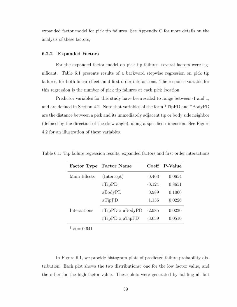
expanded factor model for pick tip failures. See Appendix C for more details on the
analysis of these factors,
6.2.2 Expanded Factors
For the expanded factor model on pick tip failures, several factors were sig-
nificant. Table 6.1 presents results of a backward stepwise regression on pick tip
failures, for both linear effects and first order interactions. The response variable for
this regression is the number of pick tip failures at each pick location.
Predictor variables for this study have been scaled to range between -1 and 1,
and are defined in Section 4.2. Note that variables of the form *TipPD and *BodyPD
are the distance between a pick and its immediately adjacent tip or body side neighbor
(defined by the direction of the skew angle), along a specified dimension. See Figure
4.2 for an illustration of these variables.
Table 6.1: Tip failure regression results, expanded factors and first order interactions
Factor Type Factor Name Coeff P-Value
Main Effects (Intercept) -0.463 0.0654
rTipPD -0.124 0.8651
aBodyPD 0.989 0.1060
aTipPD 1.136 0.0226
Interactions rTipPD x aBodyPD -2.985 0.0230
rTipPD x aTipPD -3.639 0.0510
1 φ = 0.641
In Figure 6.1, we provide histogram plots of predicted failure probability dis-
tribution. Each plot shows the two distributions: one for the low factor value, and
the other for the high factor value. These plots were generated by holding all but
59

one of the linear factors at their mean value, while allowing a single variable to range
between its high and low. The plots show a simple trend of increasing mean failure
probability with increasing factor values.
rTipPD Effects
0
0.2
0.4
0.6
0.8
1
0 1 2 3 4 5
Tip Failure Count
Pro
bab
ilit
y
Low rTipPD
High rTipPD
aBodyPD Effects
0
0.2
0.4
0.6
0.8
1
0 1 2 3 4 5
Tip Failure Count
Pro
bab
ilit
y
Low aBodyPD
High aBodyPD
aTipPD Effects
0
0.2
0.4
0.6
0.8
1
0 1 2 3 4 5 6 7 8 9 10 11 12 13 14 15
Tip Failure Count
Pro
bab
ilit
y
Low aTipPD
High aTipPD
Figure 6.1: Plot of main effects in pick tip failure regression model
Physical Interpretation – The results of the regression show a significant
connection between both tip-side and body-side angular spacing. This observation
appears to agree with theories relating frontal exposure to tip failure. Specifically,
with greater relative angular spacing, a pick is more likely to be impacted by large
pieces of broken asphalt, as they pass through the reclamation machine. As shown in
Section 2.3.3, having larger relative angular spacing also causes a pick to pass through
a larger cross-section of asphalt as it makes its cutting cycle. We expect that this
condition causes higher loads on the tip of a pick, and contributes to early failure.
An interesting result from this experiment is the discovery of interaction be-
tween relative tip height and angular spacing. Figures 6.2 and 6.3 illustrate the nature
60

of these interaction effects. For these figures, predicted mean failure rates were gen-
erated at the extreme observed values of the two interacting factors. While holding
all other factors at their mean values, we generate four response predictions from
the four possible combinations of the interacting factors. The bubbles are sized to
indicate larger or smaller response.
The particular interaction effects found to be significant, are an indication
that two modes are present in pick tip failures: sudden breakage, and abrasive wear.
Appendix C.4.1 provides additional evidence of multiple failure modes. In deep, hard
applications, pick tips appear to fail predominantly by abrasive mechanisms. An
abrasive, or wear-out failure, is evidenced by a carbide insert that is present, but has
been worn thin and flat.
Previous studies have shown that the rotation of a pick in its holder plays a
major role in prolonging pick life[4]. The USBOM study, referenced in Section 1.3.2,
found that “negative skew” was the primary contributor to pick rotation. For our
experiment, body-side angular spacing is a variant of the negative skew defined in
the USBOM study. Results from the present experiment agree with these previous
findings.
Fundamental principles of mechanical failure suggest that picks with greater
relative tip height would have shorter wear life. However, the rT ipPD × aBodyPD
interaction effect, illustrated in Figure 6.2, shows the opposite relationship. For bits
with high body-side angular spacing, relative tip height has little or no effect on tip
failure (1.28 mean failure rate vs. 0.45 mean failure rate).
Physical Interpretation – We expect that increased frontal exposure, on
the pick’s body side, would correlate well with increased rotational moment. It can
be seen from the plot of rT ipPD× aBodyPD that increased angular spacing on the
body side of the pick, combined with increased relative tip height, reduces tip failure
rate.
61
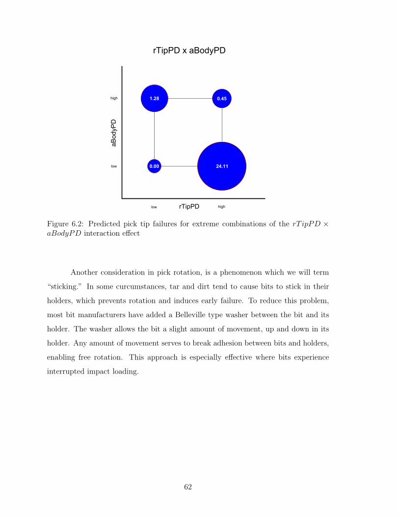
Figure 6.2: Predicted pick tip failures for extreme combinations of the rT ipPD ×aBodyPD interaction effect
Another consideration in pick rotation, is a phenomenon which we will term
“sticking.” In some curcumstances, tar and dirt tend to cause bits to stick in their
holders, which prevents rotation and induces early failure. To reduce this problem,
most bit manufacturers have added a Belleville type washer between the bit and its
holder. The washer allows the bit a slight amount of movement, up and down in its
holder. Any amount of movement serves to break adhesion between bits and holders,
enabling free rotation. This approach is especially effective where bits experience
interrupted impact loading.
62

Figure 6.3: Predicted pick tip failures for extreme combinations of the rT ipPD ×aT ipPD interaction effect
Physical Interpretation – The plot of rT ipPD× aT ipPD, in Figure 6.3, is
illustrative of bit sticking. We expect that in cases of greater tip-side angular spacing,
bits will experience a larger impact load with each revolution of the cutter head. As
explained above, this impact loading drives an increase in bit rotation. Pick wear
rate is reduced by greater relative tip height, when higher tip-side angular spacing
acts to induces pick rotation (84.42 mean failure rate vs. 0.05 mean failure rate).
6.3 Pick Body Failure Model
6.3.1 Condensed Factors
A stepwise regression for a condensed factor model on pick body failures re-
turned several significant factors. Table 6.2 presents coefficients and significance for
main and interaction effects.
63

Table 6.2: Body failure regression results for condensed factors
Factor Type Factor Name Coeff P-Value
Main Effects (Intercept) -1.148 0.0000
attack 0.816 0.1052
absSkew 1.007 0.0422
volume 1.748 0.0017
Interactions attack x volume -2.441 0.0129
1 φ = 0.898
The coefficients for this experiment indicate that pick body failures are higher
for picks with greater volume removal. Figure 6.4 shows a significant increase in
the predicted probability of failure for the observed range of per-pick volume. Picks
with high per-pick volume typically lead their neighboring picks through the cut,
which means greater exposure to both processed and intact asphalt. We also observe
that, for pick body failures, absolute skew angle (variable absSkew) has a positive
relationship to failure rate. This finding contradicts the findings of other studies[4].
However, there are two major observations that help explain this result.
Physical Interpretation – First, when operating in shallow material, picks
are engaged with the asphalt for a shorter distance on each cutting cycle. This
condition would limit the amount of rotation (in the pick holder) that each pick
experiences. By reducing the amount of rotation on each cutting cycle, the benefits
of skew angle are also reduced. Note that most pick body failures occurred in shallow
applications.
64

attack Effects
0
0.1
0.2
0.3
0.4
0.5
0.6
0.7
0.8
0.9
0 1 2 3 4 5
Body Failure Count
Pro
bab
ilit
yLow attack
High attack
absSkew Effects
0
0.2
0.4
0.6
0.8
1
0 1 2 3 4 5
Body Failure Count
Pro
bab
ilit
y
Low absSkew
High absSkew
volume Effects
0
0.2
0.4
0.6
0.8
1
1.2
0 1 2 3 4 5
Body Failure Count
Pro
bab
ilit
y
Low volume
high volume
Figure 6.4: Plot of main effects on pick body failure (condensed-factor model)
The second observation relates to pick body exposure. When a particular
bit has a larger skew angle, the body is more exposed to abrasive wear, increasing
the rate of body failures for that position. The main effects plot, Figure 6.4, for
attack angle suggests that increased attack angle is associated with increased body
exposure. However, the interaction between attack angle and per-pick volume shows
a more complex relationship.
Physical Interpretation – Figure 6.5 reveals that for bits with low volume,
attack angle does indeed increase bit failure rate. But, for bits with high per-pick
volume, greater attack angle actually decreases pick failures. This observation can
be explained by examination of Figure 2.5. Larger attack angles move the bit body
farther from the cutting interface. This change in geometry reduces body exposure to
intact asphalt, and we expect this to also reduce body exposure to processed material
flowing between pick bodies.
65
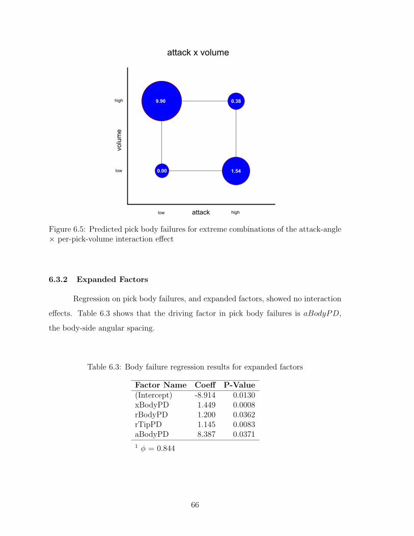
Figure 6.5: Predicted pick body failures for extreme combinations of the attack-angle× per-pick-volume interaction effect
6.3.2 Expanded Factors
Regression on pick body failures, and expanded factors, showed no interaction
effects. Table 6.3 shows that the driving factor in pick body failures is aBodyPD,
the body-side angular spacing.
Table 6.3: Body failure regression results for expanded factors
Factor Name Coeff P-Value(Intercept) -8.914 0.0130xBodyPD 1.449 0.0008rBodyPD 1.200 0.0362rTipPD 1.145 0.0083aBodyPD 8.387 0.0371
1 φ = 0.844
66

The variable, aBodyPD, is essentially a combination of skew angle and per-
pick volume. The body-side component of the variable references the skew angle.
Angular spacing is a primary contributor to per-pick volume. This finding reinforces
the conclusions of the preceding section. Additionally, body-side and tip-side variables
allow us to test the assumption that per-pick volume may have a larger effect on one
side of a pick than on the other (see Section 4.2.1). And, the results presented here
show strong evidence that this assumption is correct.
xBodyPD Effects
0
0.2
0.4
0.6
0.8
1
1.2
0 1 2
Tip Failure Count
Pro
bab
ilit
y
Low xBodypPD
High xBodyPD
rBodyPD Effects
0
0.2
0.4
0.6
0.8
1
1.2
0 1 2
Tip Failure Count
Pro
bab
ilit
y
Low rBodyPD
High rBodyPD
rTipPD Effects
0
0.2
0.4
0.6
0.8
1
1.2
0 1 2
Tip Failure Count
Pro
bab
ilit
y
Low rTipPD
High rTipPD
aBodyPD Effects
0
0.2
0.4
0.6
0.8
1
1.2
0 1 2 3 4 5
Tip Failure Count
Pro
bab
ilit
y
Low aBodyPD
High aBodyPD
Figure 6.6: Plot of main effects on pick body failure (expanded-factor model)
6.4 Contributors to Tip Radius Variation
With tip height being a strong factor in predicting bit failure, we felt it impor-
tant to analyze the sources of variation in tip height. Although direct measurement
of certain cutter head characteristics would be a more conclusive method of analyzing
tip height, we can make some definite conclusions about leading contributors.
We have identified three main sources of variation in tip height: 1) out of
round cutter head skin, 2) mis-alignment of cutter head drive plate, and 3) random
67

variation in placement of pick holders. The random height variation, resulting from
pick holder placement is apparent in Figure 6.7.
Sources of variation in pick tip height:
1. Out-of-round cutter head skin (welded pipe)
2. Mis-alignment of cutter head drive plate
3. Random variation in placement of pick holders
Figure 6.7: Plot of bit tip height and bit axial location, versus angular position
Out-of-round cutter head skin can easily be detected from direct measurements
made previously on the cutter head. Figure 6.7 shows tip height plotted against the
68

angular position of each pick around the cutter head. This plot can be interpreted
quite simply by considering the manufacturing process for large diameter pipe. This
type of pipe is rolled from sheet steel and welded. From the shape of the plot, we
can safely assume that the two ends of the pipe did not align after rolling. The
sudden change in tip height is exactly aligned with the seam in the pipe, indicating
an eccentricity problem.
Row Slope
Positive
Row Slope
Positive
CUTTER HEAD AXIS
Figure 6.8: Drawing illustrating the definition of the row slope variable
Detecting runout, resulting from a mis-aligned drive plate, proved to be more
difficult. Our analysis uses the fact that all picks are placed by pairs in rows along the
axis of the drum, with uniform angular spacing (approximately six degrees between
each row). This geometric construction is illustrated in Figure 6.8. First, we defined
a row slope variable, which is the angle between the axis of the drum and a line
69

between pick tips in a given row. Next, we compare the row slope of a given row, and
its opposing row (the row 180 degrees around the drum from the given row). If the
drive plate were mis-aligned, we would expect the row slopes to have opposite sign
for each set of opposing rows. A paired T-Test was used to determine whether the
row slopes for each set of opposing rows comes from a different population. For the
cutter head used in the present study, we failed to reject the null hypothesis, meaning
that there was no statistically detectable mis-alignment of the drive plate.
70

Chapter 7
Conclusions and Recommendations
7.1 Contributions
This research project has made significant contributions to the body of knowl-
edge surrounding tool consumption rates for construction equipment. Applications
may even be found in such fields as mining and excavating. The successful appli-
cation of observational analysis techniques to the field of engineering is particularly
noteable. The following list describes some of the major accomplishments.
• The work presented here details an effective approach to adapting statistical
methods, often applied in the fields of medicine and econometrics, to engineer-
ing problems. In particular, we have conducted a modest observational study,
but have been able to extract an amazing amount of information and insight.
We have also identified some of the limitations and potential pit-falls of using
observational experiments in engineering applications.
• As part of our study, we have developed a fast algorithm for calculating per-pick
volume removal in typical cutter head patterns. This may allow volume based
optimization of pick patterns that can be run on individual workstations, in
reasonable amounts of time. Per-pick volume also provides the designer with
a simple proxy for the complex geometrical considerations in analyzing cutter
head performance.
• Per-pick volume was the largest contributor to pick body failure. Although
per-pick volume, as presently formulated, did not appear to be a significant
71
contributor to pick tip wear, we have identified other important contributors.
The most important of these being the angular spacing between neighboring
picks. We have identified some primary sources of manufacturing variation,
and shown that they have statistically significant effect on pick wear. Recom-
mendations have been made for reducing the effect of these factors, including,
manufacturing process, lacing pattern, and pick orientation changes.
• Originally, we planned to focus our study only on pick tip failures. But, early
experimental results revealed that pick body failures accounted for a large por-
tion of overall failures. The quantifiable correlations between design parameters
and this alternate failure mode will allow cutter head designers to better tailor
their designs to specific applications.
7.2 Conclusions
Several important conclusions may be drawn from the results and analysis of
the present study. We have also made some important conclusions about observational
studies. In the following sections, we detail a few of the most significant findings:
• Three main pick failure modes are apparent in the experimental data
• Skew angle may have either a negative or positive effect on failures, depending
on application
• Pick failures follow a Poisson process
• Manufacturing variation proved to be a significant contributor to pick failure
• Observational studies can be performed with minimal resources, but should be
used with caution
7.2.1 Multiple Failure Modes
The data collected in experimentation revealed pick body failures as a signifi-
cant corollary to the pick tip failure mode. Accordingly, we developed separate models
72

for pick tip failures and pick body failures. We also presented, in Sections 6.2.2 and
C.4.1, significant evidence of multiple modes within pick tip failures: abrasive wear,
and tip breakage. These pick tip failure modes were proposed in a previous study[1],
but our analysis revealed that these modes may have different models relating them
to cutter head geometry.
7.2.2 Skew Angle Effect
Previous studies into the effects of skew angle led us to believe that greater
skew would reduce tool consumption rate. In actuality, the present study showed that
for applications in asphalt milling, skew angle can have either a negative or positive
relationship to wear. The direction of the relationship has been shown to depend on
the type of material being processed, and the relative spacing between a pick and its
axially adjacent neighbors.
Findings on skew angle touch on both design and manufacturing considera-
tions. Future cutter head designs could adjust skew angle and skew direction to im-
prove performance in a particular application. The current experiment, and resulting
models, are somewhat limited in their ability to make actual predictions. However,
with an improved model, we could revise manufacturing tolerances to reduce pick
wear resulting from variations in skew angle.
7.2.3 Pick Failures, a Poisson Process
Count data are typically modeled most effectively as a Poisson process. Al-
though the data of this experiment are somewhat underdispersed, Section C.4 presents
strong justification for the use of a Poisson model. Our analysis, using Poisson re-
gression, showed convincing statistical evidence that pick failures are indeed a pure
Poisson process.
7.2.4 Manufacturing Variation
Of the factors resulting from manufacturing variation, we found skew angle
to have very large error. As shown in Section 6.2.2, our model formulations appear
73

to have canceled the effect of this variable. However, skew angle is implicit in the
expanded factor set. The presence of proximate distance factors, in the significant
model, implies that skew angle is a contributing factor to pick tip failure. Section
6.3.1 showed that absolute skew angle was a significant contributor to pick body
failures. Accordingly, better control over the manufacturing process that orients pick
holders is likely to improve wear performance.
The findings presented in Chapter 6 showed relative tip height (rT ipPD) to
be a significant contributor to pick failure. Both failure modes that we have analyzed
show a strong correlation with pick tip radius, relative to neighboring picks. The
analysis of Section 6.4 shows that variation in cutting radius between a pick and its
neighbors results largely from runout at the pick tips. Cutter head runout is the
result of three main conditions:
1. Out of round cutter head skin
2. Mis-alignment of cutter head drive plate
3. Random variation in placement of pick holders
For the cutter head we used in this study, skin cylindricity was the largest
contributor to pick tip runout. Random variation in the placement of pick holder,
during manufacturing, was also clearly present. We were not able to detect any
statistically significant mis-alignment in the cutter head’s drive plate. From these
observations, we conclude that out-of-round cutter head skins contribute to early
pick failure.
7.2.5 Observational Studies
The use of an observational study has provided significant time and cost sav-
ings over the course of this project. We avoided having to build a special test cutter
head by taking advantage of large manufacturing variation. A designed experiment
would have required the test cutter head to be manufactured to an accuracy higher
than can be produced with current processes. In general, the deliberate perturbations
in cutter head geometry would require gage-level tolerances.
74

Observational studies represent real operating conditions. Specifically, many
different factor levels are considered when working with natural variation. This can
improve our ability to detect curvature in the response, within observed factor ranges.
Factors considered in an observational study have a smaller range of values
than would be introduced in a designed experiment. This condition acts to lowered
the significance of effects. Of course, the resulting model is also only valid for the
reduced range of observation.
When working with naturally varying data, important or influential factor
levels may not be observed. In this case, possible but unlikely states of the system are
not explored. For example, particular combinations of factor values may have never
been observed. Predictions from this type of model should be used with caution, as
predictions, even within factor ranges, may be extrapolations from the data.
The size of the sampled data set has a large influence on accuracy and validity
of results. This study had a relatively small sample size, which can lead to factor
confounding. As an example of potential confounding, a few of the picks installed in
our testing machine never failed during the experiment. In this case, we are unable
to determine whether these picks lasted longer because of variations in the picks
themselves, or because of variations in primary experiment factors. However, we can
show that pick manufacturing variation is quite small relative to the primary factors
of our experiment.
Another problem associated with small sample sizes is the increased risk of
predicting in unexplored model space. While observed data covers more of the range
for each factor, there can be unexpected gaps in the data. This may lead to inaccurate
predictions for unlikely states of the observed system.
7.3 Recommendations
The initial motivation for this study was to find the relationship between
pick tip failures and per-pick volume removal. Pick body failures were significantly
effected by volume, but we found no significant correlation with tip failures. However,
the results and analysis of Section 6.3.2 suggest that a slight variation on per-pick
75
volume would produce better results. We recommend that any further studies use
both “tip-side volume” and “body-side volume”, rather than the single variable “per-
pick volume”. This recommendation aligns with the discussion of section 4.2.1.
Based on experimental results, we recommend two separate approaches to
improving bit life: cutter head design changes, and better manufacturing controls.
Initial manufacturing improvement efforts should focus primarily on reducing
cutter head runout. This would best be accomplished by using design and production
methods that reduce the sensitivity of the assembly to variation in cutter head drum
shape. One example of this would be to turn the cutter head skin before welding the
pick mounting blocks in place. This production method would practically eliminate
pick tip runout resulting from skin runout. Random variation in the placement of
blocks could be reduced by using a gentler welding process (i.e. preheat, use short
welds, and anneal).
Design improvements to the cutter head lacing pattern are constrained by com-
peting demands. Reduction of pick tip failure rate requires greater angular spacing
on the body side, as illustrated in Figure 6.2. As described in Section 6.3.2, reduction
of pick body failure rate requires smaller angular spacing on the body side. The main
objective would therefore be to find a minimum balance between pick tip and pick
body failure rates.
In Appendix C.4, we show that pick tip failures occur in two distinct modes.
Any future experiments could easily differentiate between the two failure modes by
observing tip breakage and tip wear-out as separate events. This improvement would
provide important insights into the pick failure phenomenon.
Our final recommendation relates to future studies. One weakness in the
present study was our limited ability to account for material flow between picks. A
more complete model of material flow will be required to fully characterize the effects
of lacing pattern on pick wear. The nature of the application will probably require
some simulation, and greater efforts at direct observation.
76

Chapter 8
Future Work
This study has essentially been a screening experiment. The main purpose
of this work has been to identify factors for future study. In order to make overall
performance predictions, an in-depth designed experiment would be required. A cen-
tral composite design, similar to that performed by the USBOM[4], would require
some modification of analysis methods to be effective for count data. The significant
contributing factors, identified in this study, should be the primary focus of further
studies relating design parameters, manufacturing variation, and specific cutting ap-
plications to general tool wear rates.
8.1 Dataset Size and Randomization
Every experiment could benefit from a larger data set, and this experiment
is no exception. Specifically, we feel that the size of our dataset (number of pick
failures) is small relative to some of the random factors of Table 4.4. This weakness
could lead to a certain amount of confounding among factors. An example of potential
confounding was presented in Section 7.2. This study could help guide future studies
in the amount of testing required to achieve a certain number of pick failures.
8.2 Material Flow Between Picks
The high number of pick body failures, found in this study, suggests some ad-
ditional analysis is needed. Pick body wear failures are generally a result of processed
material flowing between picks. The factors affecting this phenomenon are not well
understood. Future efforts to understand this failure mechanism should probably
77

include both cutter head design characteristics, and asphalt material characteristics.
A list of factors, possibly affecting body failures follows.
• Material flow
– Volume of reworked material
– Clearance for material flow between picks
– Pick tip height above cutter head skin (or cutter drum)
• Pick position and orientation
– Skew angle
– Attack angle
– Pick tip radius from cutter axis of rotation
– Pattern of placement, relative to adjacent picks (or lacing pattern)
• Asphalt properties
– Aggregate size
– Matrix adhesive strength
– Asphalt temperature
– Asphalt and base material moisture content
In our experimentation, we have noticed a trend relating material flow be-
tween picks. When a patch of alligatored material is encountered (see Figure 5.1),
a number of larger pieces of asphalt are pulled through the machine, accompanied
by a significant amount of additional noise. On the read-out interval immediately
following these encounters, there appears to be an additional number of pick failures.
As discussed in Appendix C.4, two modes are apparent in pick tip failures.
We believe exploring this would be a useful extension to the current study. An
hypothetical explanation for this observation relates to lacing pattern. In most lacing
patterns, there are locations on the cutter head where the lacing pattern leaves open
78

regions or gaps. Picks that trail the gap are likely to experience larger loads when
impacted by these large pieces of processed material. We expect this to result in
premature tip failure.
8.3 Predictive Models for Pick Consumption Rate
This research lays the ground work for the development of tools that could
help road maintenance companies better manage milling machines. In particular, it
may be possible to develop an empirical model that would accurately predict ma-
chine performance and operating costs for a particular job. Inaccurate performance
predictions can be very costly, especially for contractors who have legal obligations
to meet the terms of an initial bid.
As discussed in previous sections, picks must be inspected at regular intervals.
A possible application for a general model would be to find the optimum inspection
interval, to minimize downtime.
For the present study, we have allowed the factors in Table 4.4 to vary ran-
domly, and simply observed the factors in Table 4.3. The development of a general
performance model would require explicit controls on these factors, which would add
a significant amount of effort and complexity to data collection methods.
8.4 Design Optimization
The simplified model, developed in the present study, could be adapted for
use in optimizing pick lacing patterns. Constraints on pick location, described in
Section 2.2, make this a combinatorial optimization problem. Picks are required to
be evenly spaced in both axial position and circumferential position. Only two picks
can be aligned in any allowed circumferential position. A cutter head with 94 picks
in the main pattern can be setup as an integer program consisting of 94 numbers in
varying sequence. The objective of the optimization would be to minimize variation
in wear rate between all picks. Some of the constraints on machine performance were
discussed in Section 1.1. The primary restrictions on design changes are 1) clearance
between pick holders, and 2) vibration characteristics.
79

Insufficient clearance between pick holders can make assembly difficult or im-
possible, and can prevent material flow through the pattern. These problems are
avoided by constraining the pattern to have some minimum clearance between picks,
measured in any direction. However, it may be possible to compensate for spacing
requirements by adjusting other controllable parameters. For example, irregularities
in angular spacing could be counteracted by deliberately varying tip height.
Vibration issues arise from two well-understood design problems: load imbal-
ance in the cutter head’s axial direction, and load imbalance tangent to the cutter
head. In Section 2.2, we describe a vibration problem, arising from the grouping of
picks on chevron pattern cutter heads. This grouping causes a tangential loading
imbalance, which induces an undesirable vibration mode where the milling machine
tends to bounce the entire host vehicle.
In a previous experiment, Asphalt Zipper found that designing picks to im-
pact in an alternating fashion, from left to right, induces another undesirable vibration
mode. We describe this problem as an axial loading imbalance, which causes the ma-
chine to “wag” from side-to-side. We have summarized the optimization requirements
in the following list.
Optimization definition...
• objective:
– Minimize inter-pick wear variation
• subject to:
– Lateral loading imbalance factor < Predetermined maximum value
– Tangential loading imbalance Factor < Predetermined maximum value
– Minimum pick spacing distance > Predetermined minimum value
Some combinatorial problems can be effectively solved using a branch-and-
bound method. However, this class of optimization methods require that the ob-
jective function be continuous. As currently defined, the objective function is not
80

continuous. Discontinuities in the present model arise from the the use of several
conditional evaluations on the direction of spacing. Although some statistical opti-
mization methods (i.e. genetic algorithms, or simulated annealing) would be effective,
it may be possible to simplify the model and set limits that would allow the use of
the more efficient gradient-based methods.
8.5 Variations on Volume Calculation
As shown in Section 6.2.2, per-pick volume is a weak predictor of pick tip fail-
ure, while some of the expanded factors were quite strong. This observation indicates
that the volume variable is not well formed. One alternative approach to volume
calculation would be to redefine the per-pick volume by tip-side and body-side, as
defined in Section 4.2.1. It appears, from the results of the present study, that this
approach may improve the fit of per-pick volume and greatly simplify the regression
model.
A simplified model for characterizing wear performance would allow us to im-
plement more practical optimization methods for cutter head design. The model we
have developed is much faster than using a solid modeler. But, a combinatorial opti-
mization problem with 94 parameters could still be very computationally expensive.
A central composite experimental design, on an improved per-pick volume variable,
would probably allow us to use a gradient-based optimization method.
81

82

Appendix A
Cutter Head Pattern Definitions
This appendix includes tables and plots of cutter head design and manufac-
turing information. Specifically, we have appended tables of pick position and orien-
tation, plots of pick lacing patterns, and plots of volume removal levels for 2 sizes of
cutter head. Angular measures are in radians; linear measurements are in inches.
A.1 Specifications for 30 inch Cutter Head
The following plot shows a flattened pattern for the location of bits listed in
Table A.1.
�����������
Figure A.1: Flattened plot of designed bit positions, 30 inch cutter head
The following table contains a lacing pattern specification. This specification
would be used in manufacturing 30 inch wide standard cutter heads.
83
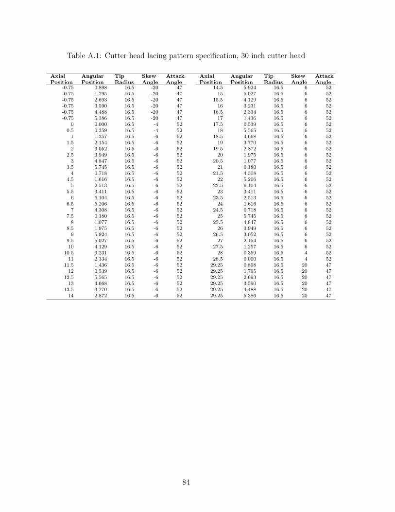
Table A.1: Cutter head lacing pattern specification, 30 inch cutter head
AxialPosition
AngularPosition
TipRadius
SkewAngle
AttackAngle
AxialPosition
AngularPosition
TipRadius
SkewAngle
AttackAngle
-0.75 0.898 16.5 -20 47 14.5 5.924 16.5 6 52-0.75 1.795 16.5 -20 47 15 5.027 16.5 6 52-0.75 2.693 16.5 -20 47 15.5 4.129 16.5 6 52-0.75 3.590 16.5 -20 47 16 3.231 16.5 6 52-0.75 4.488 16.5 -20 47 16.5 2.334 16.5 6 52-0.75 5.386 16.5 -20 47 17 1.436 16.5 6 52
0 0.000 16.5 -4 52 17.5 0.539 16.5 6 520.5 0.359 16.5 -4 52 18 5.565 16.5 6 52
1 1.257 16.5 -6 52 18.5 4.668 16.5 6 521.5 2.154 16.5 -6 52 19 3.770 16.5 6 52
2 3.052 16.5 -6 52 19.5 2.872 16.5 6 522.5 3.949 16.5 -6 52 20 1.975 16.5 6 52
3 4.847 16.5 -6 52 20.5 1.077 16.5 6 523.5 5.745 16.5 -6 52 21 0.180 16.5 6 52
4 0.718 16.5 -6 52 21.5 4.308 16.5 6 524.5 1.616 16.5 -6 52 22 5.206 16.5 6 52
5 2.513 16.5 -6 52 22.5 6.104 16.5 6 525.5 3.411 16.5 -6 52 23 3.411 16.5 6 52
6 6.104 16.5 -6 52 23.5 2.513 16.5 6 526.5 5.206 16.5 -6 52 24 1.616 16.5 6 52
7 4.308 16.5 -6 52 24.5 0.718 16.5 6 527.5 0.180 16.5 -6 52 25 5.745 16.5 6 52
8 1.077 16.5 -6 52 25.5 4.847 16.5 6 528.5 1.975 16.5 -6 52 26 3.949 16.5 6 52
9 5.924 16.5 -6 52 26.5 3.052 16.5 6 529.5 5.027 16.5 -6 52 27 2.154 16.5 6 5210 4.129 16.5 -6 52 27.5 1.257 16.5 6 52
10.5 3.231 16.5 -6 52 28 0.359 16.5 4 5211 2.334 16.5 -6 52 28.5 0.000 16.5 4 52
11.5 1.436 16.5 -6 52 29.25 0.898 16.5 20 4712 0.539 16.5 -6 52 29.25 1.795 16.5 20 47
12.5 5.565 16.5 -6 52 29.25 2.693 16.5 20 4713 4.668 16.5 -6 52 29.25 3.590 16.5 20 47
13.5 3.770 16.5 -6 52 29.25 4.488 16.5 20 4714 2.872 16.5 -6 52 29.25 5.386 16.5 20 47
84

A.2 Specifications for 48 inch Cutter Head
The following plot shows a flattened pattern for the number and location of
bits listed in Table A.2.
Figure A.2: Flattened plot of designed bit positions, 48 inch cutter head
The following table contains a lacing pattern specification. This specification
would be used in manufacturing 48 inch wide standard cutter heads.
Table A.2: Cutter head lacing pattern specification, 48 inch
Bit Axial Angular Tip Skew AttackNumber Position Position Radius Angle Angle
31 -0.75 0.0 18 23.5 4718 -0.75 120.0 18 23.5 4744 -0.75 211.8 18 23.5 471 -0.75 303.5 18 23.5 479 0 56.5 18 14.5 52
14 0.5 91.8 18 11.5 5222 1 148.2 18 6 52
85
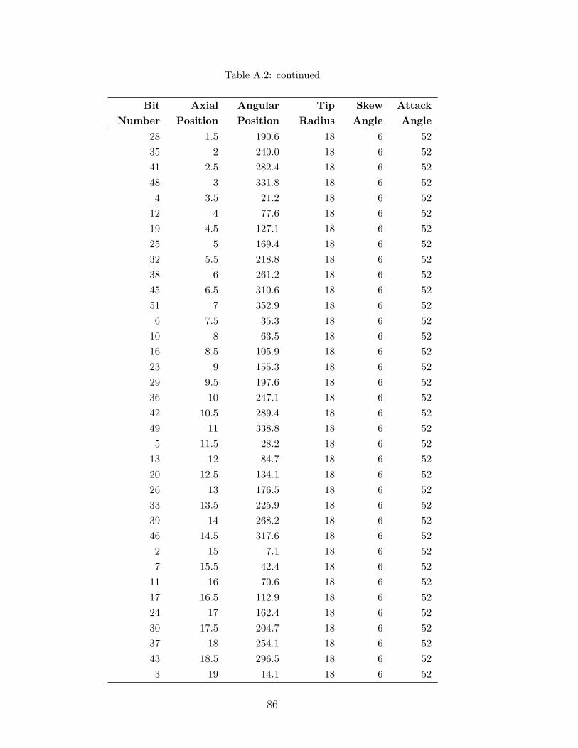
Table A.2: continued
Bit Axial Angular Tip Skew AttackNumber Position Position Radius Angle Angle
28 1.5 190.6 18 6 5235 2 240.0 18 6 5241 2.5 282.4 18 6 5248 3 331.8 18 6 524 3.5 21.2 18 6 52
12 4 77.6 18 6 5219 4.5 127.1 18 6 5225 5 169.4 18 6 5232 5.5 218.8 18 6 5238 6 261.2 18 6 5245 6.5 310.6 18 6 5251 7 352.9 18 6 526 7.5 35.3 18 6 52
10 8 63.5 18 6 5216 8.5 105.9 18 6 5223 9 155.3 18 6 5229 9.5 197.6 18 6 5236 10 247.1 18 6 5242 10.5 289.4 18 6 5249 11 338.8 18 6 525 11.5 28.2 18 6 52
13 12 84.7 18 6 5220 12.5 134.1 18 6 5226 13 176.5 18 6 5233 13.5 225.9 18 6 5239 14 268.2 18 6 5246 14.5 317.6 18 6 522 15 7.1 18 6 527 15.5 42.4 18 6 52
11 16 70.6 18 6 5217 16.5 112.9 18 6 5224 17 162.4 18 6 5230 17.5 204.7 18 6 5237 18 254.1 18 6 5243 18.5 296.5 18 6 523 19 14.1 18 6 52
86

Table A.2: continued
Bit Axial Angular Tip Skew AttackNumber Position Position Radius Angle Angle
47 19.5 324.7 18 6 5240 20 275.3 18 6 5234 20.5 232.9 18 6 5227 21 183.5 18 6 5221 21.5 141.2 18 6 5215 22 98.8 18 6 528 22.5 49.4 18 6 52
50 23 345.9 18 6 5254 23.5 14.1 18 -6 5298 24 324.7 18 -6 5291 24.5 275.3 18 -6 5285 25 232.9 18 -6 5278 25.5 183.5 18 -6 5272 26 141.2 18 -6 5266 26.5 98.8 18 -6 5259 27 49.4 18 -6 52
101 27.5 345.9 18 -6 5294 28 296.5 18 -6 5288 28.5 254.1 18 -6 5281 29 204.7 18 -6 5275 29.5 162.4 18 -6 5268 30 112.9 18 -6 5262 30.5 70.6 18 -6 5258 31 42.4 18 -6 5253 31.5 7.1 18 -6 5297 32 317.6 18 -6 5290 32.5 268.2 18 -6 5284 33 225.9 18 -6 5277 33.5 176.5 18 -6 5271 34 134.1 18 -6 5264 34.5 84.7 18 -6 5256 35 28.2 18 -6 52
100 35.5 338.8 18 -6 5293 36 289.4 18 -6 5287 36.5 247.1 18 -6 5280 37 197.6 18 -6 52
87
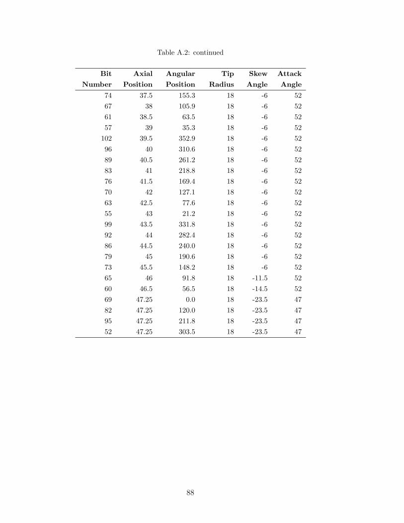
Table A.2: continued
Bit Axial Angular Tip Skew AttackNumber Position Position Radius Angle Angle
74 37.5 155.3 18 -6 5267 38 105.9 18 -6 5261 38.5 63.5 18 -6 5257 39 35.3 18 -6 52
102 39.5 352.9 18 -6 5296 40 310.6 18 -6 5289 40.5 261.2 18 -6 5283 41 218.8 18 -6 5276 41.5 169.4 18 -6 5270 42 127.1 18 -6 5263 42.5 77.6 18 -6 5255 43 21.2 18 -6 5299 43.5 331.8 18 -6 5292 44 282.4 18 -6 5286 44.5 240.0 18 -6 5279 45 190.6 18 -6 5273 45.5 148.2 18 -6 5265 46 91.8 18 -11.5 5260 46.5 56.5 18 -14.5 5269 47.25 0.0 18 -23.5 4782 47.25 120.0 18 -23.5 4795 47.25 211.8 18 -23.5 4752 47.25 303.5 18 -23.5 47
88
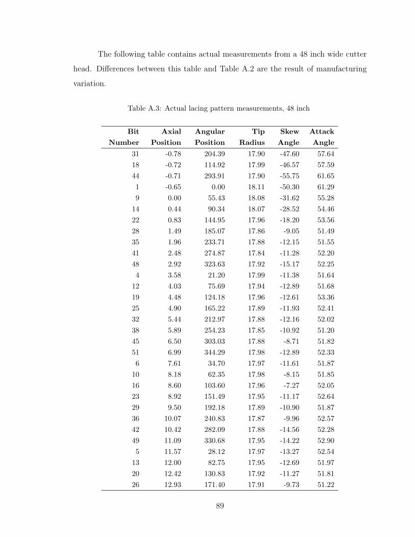
The following table contains actual measurements from a 48 inch wide cutter
head. Differences between this table and Table A.2 are the result of manufacturing
variation.
Table A.3: Actual lacing pattern measurements, 48 inch
Bit Axial Angular Tip Skew AttackNumber Position Position Radius Angle Angle
31 -0.78 204.39 17.90 -47.60 57.6418 -0.72 114.92 17.99 -46.57 57.5944 -0.71 293.91 17.90 -55.75 61.651 -0.65 0.00 18.11 -50.30 61.299 0.00 55.43 18.08 -31.62 55.28
14 0.44 90.34 18.07 -28.52 54.4622 0.83 144.95 17.96 -18.20 53.5628 1.49 185.07 17.86 -9.05 51.4935 1.96 233.71 17.88 -12.15 51.5541 2.48 274.87 17.84 -11.28 52.2048 2.92 323.63 17.92 -15.17 52.254 3.58 21.20 17.99 -11.38 51.64
12 4.03 75.69 17.94 -12.89 51.6819 4.48 124.18 17.96 -12.61 53.3625 4.90 165.22 17.89 -11.93 52.4132 5.44 212.97 17.88 -12.16 52.0238 5.89 254.23 17.85 -10.92 51.2045 6.50 303.03 17.88 -8.71 51.8251 6.99 344.29 17.98 -12.89 52.336 7.61 34.70 17.97 -11.61 51.87
10 8.18 62.35 17.98 -8.15 51.8516 8.60 103.60 17.96 -7.27 52.0523 8.92 151.49 17.95 -11.17 52.6429 9.50 192.18 17.89 -10.90 51.8736 10.07 240.83 17.87 -9.96 52.5742 10.42 282.09 17.88 -14.56 52.2849 11.09 330.68 17.95 -14.22 52.905 11.57 28.12 17.97 -13.27 52.54
13 12.00 82.75 17.95 -12.69 51.9720 12.42 130.83 17.92 -11.27 51.8126 12.93 171.40 17.91 -9.73 51.22
89

Table A.3: continued
Bit Axial Angular Tip Skew AttackNumber Position Position Radius Angle Angle
33 13.42 220.06 17.90 -11.66 53.0739 14.05 261.06 17.86 -9.75 51.0546 14.52 309.47 17.86 -8.69 51.242 15.04 7.42 18.00 -10.68 52.217 15.44 42.16 17.96 -15.49 53.07
11 15.92 69.61 17.97 -14.51 53.1917 16.49 109.75 17.95 -8.93 51.6524 16.92 158.23 17.93 -9.39 51.9830 17.36 198.89 17.91 -11.03 51.8737 17.92 247.51 17.88 -11.59 52.5543 18.42 288.37 17.90 -14.42 51.413 18.90 14.21 17.99 -10.32 51.63
47 19.47 315.95 17.90 -11.85 51.0240 19.97 268.56 17.89 -10.71 53.3934 20.49 226.77 17.89 -13.49 52.7327 20.99 178.30 17.89 -7.96 50.9521 21.50 137.42 17.89 -7.96 51.1515 22.07 96.40 17.93 -9.47 51.948 22.45 48.76 17.93 -13.48 51.95
50 22.94 337.44 17.95 -13.21 53.5354 23.43 14.31 17.95 4.85 51.0898 23.93 316.08 17.87 6.21 50.8291 24.51 268.12 17.86 9.18 52.2085 24.91 226.78 17.89 4.87 51.3778 25.38 178.10 17.88 4.94 50.7772 25.93 137.03 17.90 5.71 50.5066 26.39 96.76 17.91 3.89 51.5859 27.05 48.16 17.93 8.53 51.57
101 27.39 337.08 17.96 1.92 52.1794 27.91 288.45 17.87 6.16 50.2488 28.40 247.36 17.86 8.22 51.3181 28.83 198.64 17.90 3.73 50.9875 29.33 158.36 17.95 4.42 52.4068 29.93 109.64 17.92 6.51 51.3862 30.38 69.44 17.94 2.96 52.5958 30.87 41.83 17.94 6.20 51.75
90

Table A.3: continued
Bit Axial Angular Tip Skew AttackNumber Position Position Radius Angle Angle
53 31.30 7.58 18.01 4.75 51.1697 31.83 308.72 17.88 3.17 50.9790 32.46 261.20 17.89 8.95 52.2984 32.83 219.33 17.91 3.74 51.1277 33.41 171.58 17.91 7.07 51.1571 33.86 130.63 17.92 6.98 51.4964 34.37 82.54 17.92 5.11 51.1056 34.87 28.61 17.96 5.82 52.25
100 35.41 330.81 17.96 2.36 53.2093 35.79 281.18 17.86 3.18 50.4687 36.38 240.39 17.89 7.14 52.0680 36.88 192.26 17.92 7.48 51.8074 37.33 150.85 17.95 6.16 51.0567 37.89 103.56 17.93 7.06 52.3761 38.45 63.01 17.95 9.15 53.0757 38.87 35.24 17.95 5.40 52.49
102 39.35 343.71 17.99 3.58 52.3396 39.87 301.94 17.90 4.11 51.3889 40.47 253.64 17.87 11.59 51.1783 40.89 212.66 17.92 5.35 51.8176 41.38 164.90 17.92 6.64 51.7470 41.85 123.62 17.94 5.71 51.6963 42.34 75.97 17.89 5.55 51.5355 42.93 21.56 17.96 8.10 51.8499 43.55 322.33 17.92 7.22 50.7392 43.96 274.51 17.86 9.04 51.9186 44.33 233.34 17.89 5.87 51.2479 44.82 185.16 17.90 6.74 51.7373 45.48 144.79 17.97 8.51 52.9865 46.12 89.72 18.02 30.62 54.6160 46.51 55.03 18.02 29.31 53.9169 47.15 114.78 17.98 52.31 60.8882 47.16 204.06 17.97 44.40 56.5695 47.21 294.29 17.99 46.83 58.9452 47.22 0.34 18.08 55.20 63.46
91

92

Appendix B
Analysis Code Listings
B.1 MATLAB/Octave Per-Pick Volume Calculation
Following are the MATLAB functions and routines used to calculate the vol-
ume removed by each bit on a cutter head. The indented list, shown in Table B.1,
presents the call structure for functions used in calculating per-pick volume removal.
Code and related information for each of the functions are included in the subsequent
listings.
Table B.1: Function call structure for volume calculation
CutterApp.m
↪→ MainVolume.m
↪→ BitVolume.m
↪→ BitArea.m
↪→ Dominance.m
↪→ SectPt.m
93

Listing B.1: Main volume function - cutter head specific1 % CutterApp .m
%% SYNOPSIS% This s c r i p t c a l c u l a t e s per−pick−volume removal f o r each p ick o f a g iven% cu t t e r head . The s p e c i f i c a t i o n s f o r the cu t t e r head are pu l l e d from a
6 % comma de l im i t ed f i l e . Operat iona l parameters are d i r e c t l y ass i gned to% va r i a b l e s wi th in t h i s f i l e . Resu l t s are wr i t t en to a% constant−column−width t e x t f i l e .%% ARGUMENTS
11 % none%% INPUT% cu t t e r head s p e c i f i c a t i o n f i l e (comma de l im i t ed )% − column 1 = ax i a l p o s i t i on
16 % − column 2 = angular po s i t i on% − column 3 = arc d i s t ance po s i t i on% − column 4 = b i t t i p rad ius% − column 5 = skew ang le% − column 6 = at tack ang le
21 % − column 7 = b i t number ( from eng ineer ing drawings )% − column 8 = b i t type%% OUTPUT% column−a l i gned t e x t f i l e
26 % − column 1 = ax i a l index% − column 2 = per−pick−volume% − column 3 = ax i a l p o s i t i on% − column 4 = angular po s i t i on%
31 % OTHER VARIABLES% anaVar : de s c r i b ed in f o l l ow i n g comments% desVar : [ a x i a l p o s i t i o n , angle around drum , t i p r a d i u s ]% ppVol : [ b i t i n d e x , b i t vo lume , a x i a l p o s i t i o n , drum angle ]%
36
clear a l l ;close a l l ;
41 % ana l y s i s v a r i a b l e sVf = 8 ; % 1 forward v e l o c i t y ( f t /min) ranges from 10 to 40Wr = 150 ; % 2 angular v e l o c i t y o f c u t t i n g drum ( rev /min)Za = 75 ∗ pi /180 ; % 3 ang le o f impact a f f e c t e d zone ( rad )Ro = 0 . 0 8 ; % 4 t i p rad ius o f f s e t ( in )
46 Dc = 8 . 0 ; % 5 depth o f cut ( in )Rn = 18 ; % 6 nominal b i t rad ius ( in )Tr = 0 ; % 7 rad i a l p o s i t i o n a l t o l e rance ( in )Ta = 0 ; % 8 ax i a l p o s i t i o n a l t o l e rance ( in )Tc = 0 ; % 9 c i r cumf e r en t i a l p o s i t i o n a l t o l e rance ( in )
51 Gn = 0 . 5 ; % 10 mean gap between b i t s − pro j e c t ed onto drum ax i ss tep = 10 ; % 11 number o f vo lumetr i c i n t e g r a t i on s t ep snEB = 4 ; % 12 number o f edge b i t s per s i d e
anaVar = [ Vf ;Wr; Za ;Ro ;Dc ;Rn ; Tr ;Ta ; Tc ;Gn; s tep ;nEB ] ;56
% des ign v a r i a b l e s [ a x i a l p o s i t i o n , angle around drum , t i p r a d i u s ]inData = dlmread( ’ 48 Locator 2005 −08−31. csv ’ ) ;inData = sort rows ( inData , 1 ) ;
desVar = [ inData ( : , 1 ) , inData ( : , 2 ) , inData ( : , 4 ) ] ;61 nBits = s ize ( desVar , 1) ;
% ppVol = [ b i t i n d e x , b i t vo lume , a x i a l p o s i t i o n , drum angle ]ppVol = MainVolume ( desVar , anaVar ) ;ppVol = sor t rows ( ppVol , [ 3 , 4 ] ) ;
66
save −a s c i i 48 l o ca to r−ppvol 2005 −08−31. txt ppVol
disp ( ’ b i t i nd ex bit vo lume a x i a l p o s i t i o n drum angle ’ ) ;disp ( ppVol ) ;
94

Listing B.2: Main Volume Calculation Routine% MainVolume .m%% SYNOPSIS% This func t i on c a l c u l a t e s volume of mater ia l removed by each cu t t e r ,
5 % neg l e c t i n g forward movement o f machine wh i l e b i t i s engaged%% ARGUMENTS% desVar : an array o f b i t po s i t i on s , SORTED BY AXIAL POSITION, con s i s t i n g o f% − column 1 = ax i a l p o s i t i on o f b i t , measured from edge o f sk in
10 % − column 2 = angular po s i t i on o f b i t measured from drum ’ s weld seam% − column 3 = rad ius o f b i t t i p from drum ax i s% anaVar : a vec tor o f machine parameters (more d e t a i l s below )%% OUTPUT
15 % volArray : An array o f b i t s , by index , wi th volume , a x i a l pos i t i on , and drum% ang le . Inc ludes a l l b i t s , but has NaN va lue s f o r b i t s t ha t% exper ience edge e f f e c t s ( edge b i t s , and b i t s t ha t dominate edge% b i t s ) .% − column 1 = index based on increa s ing a x i a l p o s i t i on
20 % − column 2 = per−pick−volume fo r each b i t% − column 3 = ax i a l p o s i t i on o f b i t , measured from edge o f sk in% − column 4 = angular po s i t i on o f b i t measured from drum ’ s weld seam%% OTHER VARIABLES
25 % bi tPa t t e rn : [ a x i a l p o s i t i o n , angle around drum , t i p r ad i u s , machine advance ]% ordBi ts : [ a x i a l p o s i t i o n i n d e x , angle around drum ]%% REVISION HISTORY% changed 2005−01−28:
30 % removed automatic d e t e c t i on o f number o f edge b i t s% added a var i ab l e , s e t by the user , f o r the number o f edge b i t s%% changed 2005−12−13:% changed volArray from
35 % [ ax i a l i nde x , b i t vo lume , a x i a l p o s i t i o n , machine advance ]% to% [ ax i a l i nde x , b i t vo lume , a x i a l p o s i t i o n , drum angle ]%% changed 2006−01−26:
40 % changed return va lue to inc lude a l l b i t s , wi th NaN for the volume% of non−c a l c u l a t e d edge b i t s%
function volArray = MainVolume ( desVar , anaVar )45
% name the ana l y s i s v a r i a b l e sVf = anaVar (1 ) ; % 1 forward v e l o c i t y ( f t /min) ranges from 10 to 40Wr = anaVar (2 ) ; % 2 angular v e l o c i t y o f c u t t i n g drum ( rev /min)Za = anaVar (3 ) ; % 3 ang le o f impact a f f e c t e d zone ( rad )
50 Ro = anaVar (4 ) ; % 4 t i p rad ius o f f s e t ( in )Dc = anaVar (5 ) ; % 5 depth o f cut ( in )Rn = anaVar (6 ) ; % 6 nominal b i t rad ius ( in )Tr = anaVar (7 ) ; % 7 rad i a l p o s i t i o n a l t o l e rance ( in )Ta = anaVar (8 ) ; % 8 ax i a l p o s i t i o n a l t o l e rance ( in )
55 Tc = anaVar (9 ) ; % 9 c i r cumf r en t i a l p o s i t i o n a l t o l e rance ( in )Gn = anaVar (10) ; % 10 average gap between b i t s ( p ro j e c t ed onto drum ax i s )s tep = anaVar (11) ; % 11 number o f vo lumetr i c i n t e g r a t i on s t ep snEB = anaVar (12) ; % 12 number o f edge b i t s
60 nBits = s ize ( desVar , 1 ) ;
% ana l y s i s f unc t i on s65
% forward v e l o c i t y ( in /min)anaParam . Vi = Vf ∗ 12 ;
% rad/min70 anaParam .Wa = Wr∗2∗pi ;
95

% depth o f cutanaParam .Dc = Dc ;
75 % advance per r e vo l u t i on ( in )anaParam . Ar = anaParam . Vi/Wr;
% ang le from the nega t i v e o f the advance d i r e c t i on to the cut e x i t ang leanaParam .bMax = acos ( (Rn−Dc) /Rn) + pi /2 ;
80
% maximum domination index d i f f e r e n c eDdMax = (Rn + Tr) − (Rn−Tr) ∗( sin ( pi − . . .
asin ( anaParam . Ar/(Rn−Tr) ∗ sin ( anaParam .bMax) ) − . . .anaParam .bMax) / sin ( anaParam .bMax) ) ;
85 maxDomDist = DdMax/tan ( pi/2 − Za/2) ;anaParam . maxDomIndex = ce i l (maxDomDist/(Gn − 2∗Ta) ) ;
% ang le o f s i d e o f cut p r o f i l e in the f l a t p laneanaParam . domAngle = pi/2 − Za /2 ;
90
% s lope o f s i d e o f cut p r o f i l e in the f l a t p laneanaParam . domSlope = tan ( anaParam . domAngle ) ;
% l i s t o f r o t a t i on ang l e s at which to eva lua t e b i t cross−s e c t i on s95 s ta r tAng l e = pi /2 ;
stepAng = (anaParam .bMax − s ta r tAng l e ) /( s tep − 1) ;eva lAngles = star tAng l e : stepAng : anaParam .bMax ;
anaParam . eva lAng les = evalAngles ’ ; % ( transposed )
100 % arc d i s t ance between b i t cross−s e c t i on sanaParam . stepArc = Rn ∗ stepAng ;
% l i s t o f r a d i i to a spha l t sur face , a long each eva lAng les d i r e c t i onanaParam . surfRad = ( (Rn + Ro) − Dc) . / cos ( anaParam . eva lAng les − pi /2) ;
105
% edges o f cut ( l e f tmo s t and r igh tmos t b i t s )anaParam . edge = [min( desVar ( : , 1 ) ) ,max( desVar ( : , 1 ) ) ] ;
110
% add machine advance d i s t ance at each b i t ’ s impact% [ a x i a l d i s t , drum angle , t i p r ad i u s , machine advance ]
b i tPat te rn = [ desVar , ( anaParam . Vi ∗ desVar ( : , 2 ) / anaParam .Wa) ] ;
115 % add t i p rad ius o f f s e t to b i t r a d i i ( accounts f o r rounded t i p on b i t )b i tPat te rn ( : , 3 ) = b i tPat te rn ( : , 3 ) + Ro ;
% add a x i a l i n d e x and so r t b i t s by order o f impact% ordBi ts = [ ax i a l i nde x , drum angle ]
120 ordBit s = [ ( 1 : nBits ) ’ , b i tPat t e rn ( : , 2 ) ] ;o rdBit s = sor t rows ( ordBits , 2 ) ;
125 % step through b i t s in order o f impactbitVolArray = [ ] ;lastAdvance = 0 ;for j = 1 : nBits
130 % get next impact b i t and make current (move b i t forward to 2nd drum rev )currBi t Index = ordBit s ( j , 1 ) ; % next b i t a x i a l i n d e xcurrBitData = bi tPat t e rn ( currBitIndex , : ) ; % next b i t data rowcurrBitData (4 ) = currBitData (4 ) + anaParam . Ar ; % move next b i t forward
135 % i f not an edge b i t , c a l l volume func t ion and add to b i t volume arrayi f ( currBi t Index > nEB + 1) && ( currBi t Index < nBits−nEB)
bi tVo l = BitVolume ( b i tPattern , currBit Index , currBitData , anaParam) ;bitVolArray = [ bitVolArray ;
currBit Index , bitVol , currBitData (1 ) , currBitData (2 ) ] ;140 else
bitVolArray = [ bitVolArray ;currBit Index , NaN, currBitData (1 ) , currBitData (2 ) ] ;
end
96

145 % update b i t pa t t e rn to new po s i t i on o f current b i tb i tPat te rn ( currBit Index , : ) = currBitData ;
end
150 volArray = bitVolArray ;
97

Listing B.3: Single Pick Volume Routine% BitVolume .m%% SYNOPSIS
4 % Receives data f o r a s i n g l e b i t l o ca t i on , and re turns i t s cut volume .%% ARGUMENTS% b i tPa t t e rn : an array o f b i t po s i t i on s , sor t ed by a x i a l p o s i t i on :% − column 1 = ax i a l p o s i t i on o f b i t , measured from edge o f sk in
9 % − column 2 = angular po s i t i on o f b i t measured from drum ’ s weld seam% − column 3 = rad ius o f b i t t i p from drum ax i s ( ye t to come)% − column 4 = machine advance d i s t ance s ince s t a r t o f t h i s r e vo l u t i on% currBi t Index : index po s i t i on o f current b i t in b i tPa t t e rn ( prev rev )% currBitData : l i s t o f data f o r current b i t in advanced po s i t i on ( curr rev )
14 % anaParam : l i s t o f ana l y s i s paramaters and func t i on s f o r the machine%% OUTPUT% bi tVo l : volume of mater ia l removed by the b i t at currentBi t Index%
19 % OTHER VARIABLES% se c tB i t s : A sub s e t o f the main b i tPa t t e rn data , conta in ing b i t s w i th in% dominance range o f the current b i t . This avo ids having to search% a l l b i t s f o r dominance .%
24
function bi tVo l = BitVolume ( b i tPattern , currBit Index , currBitData , anaParam)
l im i tL = currBi t Index − 2 ∗ anaParam . maxDomIndex ;29 i f l im i tL < 1
l im i tL = 1 ;endl imitR = currBi t Index + 2 ∗ anaParam . maxDomIndex ;i f l imitR > s ize ( b i tPattern , 1 )
34 l imitR = s ize ( b i tPattern , 1 ) ;ends e c tB i t s = b i tPat te rn ( l im i tL : l imitR , : ) ;
% open f i l e f o r debugging39 %f i d = fopen ( ’ area debug1 . t x t ’ , ’ a+t ’ ) ;
%f p r i n t f ( f i d , ’%10.6 f \ t ’ , b i tPa t t e rn ( currBitIndex , 1 ) ) ;
% c a l c u l a t e current b i t ’ s volumebi tVo l = 0 ;
44 currBitArea = 0 ;for i = 1 : ( s ize ( anaParam . evalAngles , 1 ) )
% get next b i t ’ s volumenextBitArea = BitArea ( s e c tB i t s , currBitData , anaParam , . . .
49 anaParam . eva lAng les ( i ) , anaParam . surfRad ( i ) ) ;
% cen t r a l d i f f e r e n c e i n t e g r a t e f o r t h i s segment o f volumebi tVo l = bitVol + anaParam . stepArc ∗ ( nextBitArea + currBitArea ) /2 ;
54 % s h i f t next area to current areacurrBitArea = nextBitArea ;
% pr in t debug in f o%f p r i n t f ( f i d , ’%10.6 f \ t ’ , currBitArea ) ;
59
end
% c l o s e debugging f i l e%f p r i n t f ( f i d , ’\n ’ ) ;
64 %f c l o s e ( f i d ) ;
98

Listing B.4: Calculate Single Pick Cut Cross-Section1 % BitArea .m
%% SYNOPSIS% This func t i on r e c e i v e s a b i t array and current b i t index , and re turns the% cross−s e c t i o n a l area o f the mater ia l removal zone f o r the s p e c i f i e d b i t at
6 % the s p e c i f i e d ang le .%% Green ’ s Theorem%% 1 n / \
11 % area = − SUM ( x [ i ] y [ i +1] − x [ i +1] y [ i ] )% 2 i=1 \ /%% re f e rence page 9 o f l a b notebook fo r more d e t a i l s%
16 % ARGUMENTS% se c tB i t s : an array o f b i t po s i t i on s , so r t ed by a x i a l p o s i t i on :% − column 1 = ax i a l p o s i t i on o f b i t , measured from edge o f sk in% − column 2 = angular po s i t i on o f b i t measured from drum ’ s weld seam% − column 3 = rad ius o f b i t t i p from drum ax i s ( ye t to come)
21 % − column 4 = machine advance d i s t ance s ince s t a r t o f t h i s r e vo l u t i on% currBitData : l i s t o f data f o r current b i t in advanced po s i t i on ( curr rev )% anaParam : l i s t o f ana l y s i s paramaters and func t i ons f o r the machine% currAngle : ang le o f r o t a t i on fo r current b i t% surfRad : rad ius to a spha l t sur face , a long currAngle
26 %% OUTPUT% bitArea : cross−s e c t i o n a l area o f the current b i t ’ s cut , at the current% cu t t e r head ang le o f r o t a t i on%
31 % OTHER VARIABLES% b i t S e c t 3 : sub s e t o f s e c tB i t s , conta in ing b i t s not dominated by any other b i t% in sec tB i t s , or by current b i t% sec tP t s : s e t o f x , y coord ina te s f o r i n t e r s e c t i o n po in t s between cut% p r o f i l e s o f a l l b i t s ( f o r green ’ s theorem )
36 %
function bitArea = BitArea ( s e c tB i t s , currBitData , anaParam , currAngle , surfRad )
41
% i n i t i a l i z e v a r i a b l e snSect1 = s ize ( s e c tB i t s , 1 ) ;s e c tPt s = [ currBitData (1 ) , currBitData (3 ) ] % coords o f 1 s t v e r t e x [ x , y ]bitArea = 0 ;
46
% f ind r e l a t i v e depths (Dr) f o r the sub s e t o f b i t sR = se c tB i t s ( : , 3 ) ; % co l vec to r o f r a d i iA = currBitData (4 ) − s e c tB i t s ( : , 4 ) ; % co l vec to r o f advance d i s t ance sb = currAngle ;
51 Dr = R .∗ ( sin ( pi − asin (A . / R .∗ sin (b) ) − b) / sin (b) ) ;b i tS e c t 1 = [ s e c tB i t s , Dr ] ;b i tS e c t 3 = [ ] ;
56
% Generate a sub s e t o f non dominated b i t sfor i = 1 : nSect1
domChk = 0 ;61 % f ind domination l im i t s
lowLim = i − anaParam . maxDomIndex ;hiLim = i + anaParam . maxDomIndex ;i f i <= anaParam . maxDomIndex
lowLim = 1 ;66 e l s e i f i >= ( nSect1 − anaParam . maxDomIndex)
hiLim = nSect1 ;end
% f ind dominated b i t s71 for j = lowLim : hiLim
99

i f ( i ˜= j )i f Dominance ( b i tS e c t 1 ( i , [ 1 , 5 ] ) , b i tS e c t 1 ( j , [ 1 , 5 ] ) , . . .
anaParam . domAngle ) == 1domChk = 1 ;
76 break ;end
endend
81 % wri t e non−dominated b i t s to an arrayi f domChk == 0
i f b i tS e c t 1 ( i , 5 ) > surfRadb i tS e c t 3 = [ b i tS e c t 3 ; b i tS e c t 1 ( i , : ) ] ;
else86 % inc lude the b i t anyway fo r the qu ick and d i r t y method ( to
% be changed l a t e r )b i tS e c t 3 = [ b i tS e c t 3 ; b i tS e c t 1 ( i , : ) ] ;
endend
91
end
96 nSect2 = s ize ( b i tSect3 , 1 ) ;lastDomChk = 0 ;
for i = 1 : nSect2
101 % righ t−most b i t ( t h i s b i t to the r i g h t o f the current b i t , and not% dominated by the current b i t )
i f b i tS e c t 3 ( i , 1 ) > currBitData (1 )i f Dominance ( b i tS e c t 3 ( i , [ 1 , 5 ] ) , currBitData ( [ 1 , 3 ] ) , . . .
anaParam . domAngle ) == 0106 % in t e r s e c t i o n − t h i s b i t and new b i t
newSectPt = SectPt ( currBitData ( [ 1 , 3 ] ) , b i tS e c t 3 ( i , [ 1 , 5 ] ) , . . .anaParam . domSlope ) ;
%i f newSectPt (2) < surfRad% change the i n t e r s e c t i o n po in t to be with the sur face
111 % of the aspha l t , ra ther than with the ne ighbor ing b i t%endbitArea = bitArea . . .
+ ( s e c tPt s ( s ize ( sectPts , 1) , 1) ∗newSectPt (2 ) . . .− newSectPt (1 ) ∗ s e c tPt s ( s ize ( sectPts , 1) , 2) ) ;
116 s e c tPt s = [ s e c tPt s ; newSectPt ] ;break ;
endend
121 % non−dominated b i t si f Dominance ( b i tS e c t 3 ( i , [ 1 , 5 ] ) , currBitData ( [ 1 , 3 ] ) , . . .
anaParam . domAngle ) == 0
% l e f t −most b i t ( t h i s b i t not dominated , next b i t dominated , or126 % a f t e r the current b i t )
i f (Dominance ( b i tS e c t 3 ( i +1 , [ 1 , 5 ] ) , currBitData ( [ 1 , 3 ] ) , . . .anaParam . domAngle ) == 1) | | ( b i tS e c t 3 ( i +1 ,1) > currBitData (1 ) ) ;
% in t e r s e c t i o n − t h i s b i t and new b i t131 newSectPt = SectPt ( b i tS e c t 3 ( i , [ 1 , 5 ] ) , currBitData ( [ 1 , 3 ] ) , . . .
anaParam .domSlope) ;
b itArea = bitArea + . . .( s e c tPt s ( s ize ( sectPts , 1) , 1) ∗newSectPt (2 ) − . . .newSectPt (1 ) ∗ s e c tPt s ( s ize ( sectPts , 1) , 2) ) ;
136 s e c tPt s = [ s e c tPt s ; newSectPt ] ;
% in t e r s e c t i o n − t h i s b i t and next b i tnewSectPt = SectPt ( b i tS e c t 3 ( i , [ 1 , 5 ] ) , b i tS e c t 3 ( i +1 , [ 1 , 5 ] ) , . . .
anaParam . domSlope ) ;141 bitArea = bitArea + . . .
( s e c tPt s ( s ize ( sectPts , 1) , 1) ∗newSectPt (2 ) − . . .
100
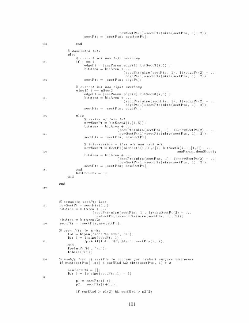
newSectPt (1 ) ∗ s e c tPt s ( s ize ( sectPts , 1) , 2) ) ;s e c tPt s = [ s e c tPt s ; newSectPt ] ;
146 end
% dominated b i t selse
% current b i t has l e f t overhang151 i f i == 1
edgePt = [ anaParam . edge (1 ) , b i tS e c t 3 ( i , 5 ) ] ;b i tArea = bitArea + . . .
( s e c tPt s ( s ize ( sectPts , 1) , 1) ∗ edgePt (2 ) − . . .edgePt (1 ) ∗ s e c tPt s ( s ize ( sectPts , 1) , 2) ) ;
156 s e c tPt s = [ s e c tPt s ; edgePt ] ;
% current b i t has r i g h t overhange l s e i f i == nSect2
edgePt = [ anaParam . edge (2 ) , b i tS e c t 3 ( i , 5 ) ] ;161 bitArea = bitArea + . . .
( s e c tPt s ( s ize ( sectPts , 1) , 1) ∗ edgePt (2 ) − . . .edgePt (1 ) ∗ s e c tPt s ( s ize ( sectPts , 1) , 2) ) ;
s e c tPt s = [ s e c tPt s ; edgePt ] ;
166 else% ver t e x o f t h i s b i tnewSectPt = b i tSe c t 3 ( i , [ 1 , 5 ] ) ;b itArea = bitArea + . . .
( s e c tPt s ( s ize ( sectPts , 1) , 1) ∗newSectPt (2 ) − . . .171 newSectPt (1 ) ∗ s e c tPt s ( s ize ( sectPts , 1) , 2) ) ;
s e c tPt s = [ s e c tPt s ; newSectPt ] ;
% in t e r s e c t i o n − t h i s b i t and next b i tnewSectPt = SectPt ( b i tS e c t 3 ( i , [ 1 , 5 ] ) , b i tS e c t 3 ( i +1 , [ 1 , 5 ] ) , . . .
176 anaParam . domSlope ) ;b itArea = bitArea + . . .
( s e c tPt s ( s ize ( sectPts , 1) , 1) ∗newSectPt (2 ) − . . .newSectPt (1 ) ∗ s e c tPt s ( s ize ( sectPts , 1) , 2) ) ;
s e c tPt s = [ s e c tPt s ; newSectPt ] ;181 end
lastDomChk = 1 ;end
end186
% complete s ec tP t s loop191 newSectPt = sec tPt s ( 1 , : ) ;
b i tArea = bitArea + . . .( s e c tPt s ( s ize ( sectPts , 1) , 1) ∗newSectPt (2 ) − . . .newSectPt (1 ) ∗ s e c tPt s ( s ize ( sectPts , 1) , 2) ) ;
b itArea = bitArea /2 ;196 s e c tPt s = [ s e c tPt s ; newSectPt ] ;
% open f i l e to wr i t ef i d = fopen ( ’ s e c tPt s . txt ’ , ’ a ’ ) ;for i = 1 : s ize ( sectPts , 1 )
201 fpr intf ( f i d , ’%f \ t%f \n ’ , s e c tPt s ( i , : ) ) ;endfprintf ( f i d , ’ \n ’ ) ;fc lose ( f i d ) ;
206 % modify l i s t o f s e c tP t s to account f o r a spha l t sur face emergencei f min( s e c tPt s ( : , 2 ) ) < surfRad && s ize ( sectPts , 1) > 2
newSectPts = [ ] ;for i = 1 : ( s ize ( sectPts , 1 ) − 1)
211
p1 = sec tPt s ( i , : ) ;p2 = sec tPt s ( i +1 , : ) ;
i f surfRad > p1 (2) && surfRad > p2 (2)
101

216 %do nothinge l s e i f surfRad < p1 (2) && surfRad < p2 (2)
%add poin t p1 to the new arraynewSectPts = [ newSectPts ; p1 ] ;
e l s e i f p1 (2) > surfRad && surfRad > p2 (2)221 %f ind the i n t e r s e c t i o n between surfRad and vec tor [ p1 , p2 ]
newSectX = p1 (1) + . . .( surfRad − p1 (2) ) ∗( p2 (1 ) − p1 (1) ) /( p2 (2 ) − p1 (2) ) ;
%add p1 and i n t e r s e c t i o n to the new array in ordernewSectPts = [ newSectPts ; p1 ; [ newSectX , surfRad ] ] ;
226 e l s e i f p2 (2) > surfRad && surfRad > p1 (2)%f ind the i n t e r s e c t i o n between surfRad and vec tor [ p1 , p2 ]newSectX = p1 (1) + . . .
( surfRad − p1 (2) ) ∗( p2 (1 ) − p1 (1) ) /( p2 (2 ) − p1 (2) ) ;%add i n t e r s e c t i o n to the new array
231 newSectPts = [ newSectPts ; [ newSectX , surfRad ] ] ;else
% errorend
236 end
% implement green ’ s theorem , i f any non−dominated area e x i s t si f s ize ( newSectPts , 1 ) == 0
bitArea = 0 ;241 else
newSectPts = [ newSectPts ; newSectPts ( 1 , : ) ] ;newBitArea = 0 ;for i = 1 : ( s ize ( newSectPts , 1) − 1)
% port ion o f formula i n s i d e the sum : x [ i ] y [ i +1] − x [ i +1] y [ i ]246 newBitArea = newBitArea + . . .
( newSectPts ( i , 1) ∗newSectPts ( i +1 ,2) − . . .newSectPts ( i +1 ,1)∗newSectPts ( i , 2 ) ) ;
endbitArea = newBitArea / 2 ;
251
end
end
102

Listing B.5: Determine Pick Domination1 % Dominance .m
%% SYNOPSIS% This func t i on take s the po s i t i on o f two b i t t i p s , and determines whether% one i s dominated by the other . The f i r s t b i t i s dominated i f the second b i t
6 % has removed i t ’ s mater ia l on an e a r l i e r pass .%% ARGUMENTS% pos1 : Coordinate s e t f o r b i t 1 t i p l o c a t i on% − element 1 = ax i a l ( x ) t i p po s i t i on o f b i t 1
11 % − element 2 = rad i a l ( y ) t i p po s i t i on o f b i t 1% pos2 : Coordinate s e t f o r b i t 1 t i p l o c a t i on% − element 1 = ax i a l ( x ) t i p po s i t i on o f b i t 2% − element 2 = rad i a l ( y ) t i p po s i t i on o f b i t 2% domAngle : S lope o f the cut p r o f i l e ( r i s e /run in the p lane o f the current
16 % b i t s rad ius vec to r )%% OUTPUT% dominated : i n t e g e r va lue% 0 = b i t 1 i s NOT dominated by b i t 2
21 % 1 = b i t 1 i s dominated by b i t 2%
function dominated = Dominance ( pos1 , pos2 , domAngle )
26 compAngle = atan2 ( ( pos2 (2 ) − pos1 (2 ) ) , ( pos2 (1 ) − pos1 (1 ) ) ) ;
i f ( compAngle > domAngle ) && ( compAngle < ( pi − domAngle ) )dominated = 1 ;
else31 dominated = 0 ;
end
103

Listing B.6: Pick Path Intersection Coordinates% SectPt .m%
3 % SYNOPSIS% This func t i on take s the po s i t i on o f two b i t t i p s , and f i n d s the coord ina te s% the coord ina te s at which the cut p r o f i l e s o f each b i t i n t e r s e c t .% NOTE: Bit arguments ( b i t p o s i t i on vec tor o b j e c t s ) must be supp l i e d in l e f t% to r i g h t order ( i . e . the b i t wi th the sma l l e r x must be passed as
8 % the f i r s t argument )%% ARGUMENTS% ( r i s e /run in the p lane o f the current b i t s rad ius vec tor )% pos1 : Coordinate s e t f o r b i t 1 t i p l o c a t i on
13 % − element 1 = ax i a l ( x ) t i p po s i t i on o f b i t 1% − element 2 = rad i a l ( y ) t i p po s i t i on o f b i t 1% pos2 : Coordinate s e t f o r b i t 1 t i p l o c a t i on% − element 1 = ax i a l ( x ) t i p po s i t i on o f b i t 2% − element 2 = rad i a l ( y ) t i p po s i t i on o f b i t 2
18 % domAngle : S lope o f the cut p r o f i l e ( r i s e /run in the p lane o f the current% b i t s rad ius vec to r )%% OUTPUT% sectArray : x−y coord inate po s i t i on o f the i n t e r s e c t i o n between the two
23 % b i t s ’ cut p r o f i l e%
function sectArray = SectPt ( pos1 , pos2 , cutS lope )28
% swi tch the s i gn o f the cutS lope , s ince the l e f t b i t i s always f i r s tcutS lope = −cutS lope ;
% f ind the x coord inate33 x = ( ( pos2 (2 ) + cutS lope ∗pos2 (1 ) ) − ( pos1 (2 ) − . . .
cutS lope ∗pos1 (1 ) ) ) /(2∗ cutS lope ) ;
% the y coord inate i s found from the x coord inatey = cutS lope ∗x + ( pos1 (2 ) − cutS lope ∗pos1 (1 ) ) ;
38
% return the coord inate arraysectArray = [ x , y ] ;
104
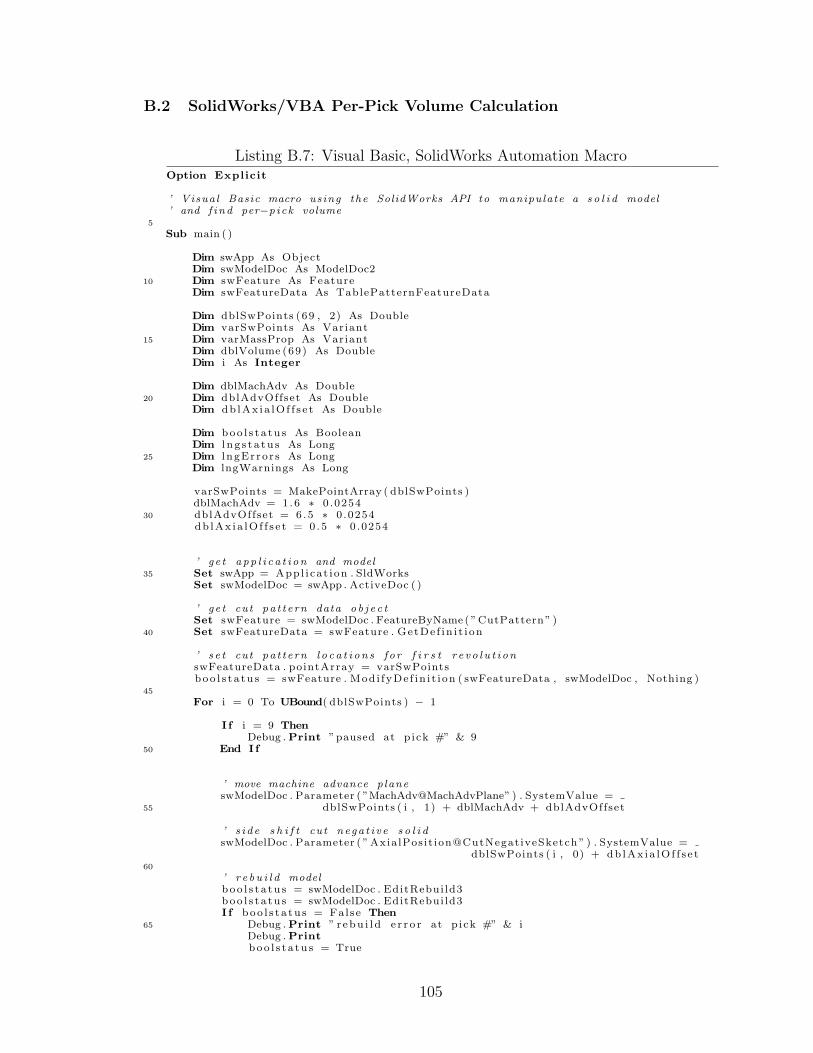
B.2 SolidWorks/VBA Per-Pick Volume Calculation
Listing B.7: Visual Basic, SolidWorks Automation MacroOption Explicit
’ Visua l Basic macro us ing the SolidWorks API to manipulate a s o l i d model’ and f i nd per−p ick volume
5
Sub main ( )
Dim swApp As ObjectDim swModelDoc As ModelDoc2
10 Dim swFeature As FeatureDim swFeatureData As TablePatternFeatureData
Dim dblSwPoints (69 , 2) As DoubleDim varSwPoints As Variant
15 Dim varMassProp As VariantDim dblVolume (69) As DoubleDim i As Integer
Dim dblMachAdv As Double20 Dim dblAdvOffset As Double
Dim db lAx ia lO f f s e t As Double
Dim boo l s t a tu s As BooleanDim l n g s t a tu s As Long
25 Dim l ngEr ro r s As LongDim lngWarnings As Long
varSwPoints = MakePointArray ( dblSwPoints )dblMachAdv = 1 .6 ∗ 0 .0254
30 dblAdvOffset = 6 .5 ∗ 0 .0254db lAx i a lO f f s e t = 0 .5 ∗ 0 .0254
’ g e t a pp l i c a t i on and model35 Set swApp = Appl i ca t ion . SldWorks
Set swModelDoc = swApp . ActiveDoc ( )
’ g e t cut pa t t e rn data o b j e c tSet swFeature = swModelDoc . FeatureByName ( ”CutPattern” )
40 Set swFeatureData = swFeature . GetDe f in i t i on
’ s e t cut pa t t e rn l o c a t i on s f o r f i r s t r e v o l u t i onswFeatureData . pointArray = varSwPointsboo l s t a tu s = swFeature . Mod i fyDe f in i t i on ( swFeatureData , swModelDoc , Nothing )
45
For i = 0 To UBound( dblSwPoints ) − 1
I f i = 9 ThenDebug . Print ”paused at p ick #” & 9
50 End I f
’ move machine advance planeswModelDoc . Parameter ( ”MachAdv@MachAdvPlane” ) . SystemValue =
55 dblSwPoints ( i , 1) + dblMachAdv + dblAdvOffset
’ s i d e s h i f t cut nega t i v e s o l i dswModelDoc . Parameter ( ”AxialPos it ion@CutNegat iveSketch ” ) . SystemValue =
dblSwPoints ( i , 0) + db lAx i a lO f f s e t60
’ r e b u i l d modelboo l s t a tu s = swModelDoc . EditRebui ld3boo l s t a tu s = swModelDoc . EditRebui ld3I f boo l s t a tu s = False Then
65 Debug . Print ” r ebu i l d e r r o r at p ick #” & iDebug . Printboo l s t a tu s = True
105

End I f
70 ’ g e t volumevarMassProp = swModelDoc . Extension . GetMassPropert ies (1 , l n g s t a tu s )dblVolume ( i ) = varMassProp (3 )
’ pause execu t ion fo r s p e c i a l b i t s75 I f i = 22 Or i = 49 Then
Debug . Print ”paused f o r model check ing at p ick #” & iDebug . Print
End I f
80 ’ ad ju s t pa t t e rn array f o r new cut po s i t i onvarSwPoints ( i ∗ 3 + 1) = varSwPoints ( i ∗ 3 + 1) + dblMachAdvswFeatureData . pointArray = varSwPoints
’ r e s e t cut pa t t e rn l o c a t i on s85 boo l s t a tu s = swFeature . Mod i fyDe f in i t i on ( swFeatureData ,
swModelDoc , Nothing )I f boo l s t a tu s = False Then
Debug . Print ” pattern update e r r o r at p ick #” & iDebug . Print
90 boo l s t a tu s = TrueEnd I f
Next i
95 Debug . Print ” ax ia l , machadv , volume”For i = 0 To UBound( dblVolume ) − 1
Debug . Print dblSwPoints ( i , 0) & ” , ” & dblSwPoints ( i , 1) &” , ” & dblVolume ( i )
Next i100
End Sub
105 Function MakePointArray ( dblArray ( ) As Double ) As Variant’ db lArray i s an empty , s i z e d array’ array va lue s i n s e r t e d here as a quick−and−d i r t y method’ f o r g r ea t e r f l e x i b i l i t y , the va lue s shou ld be loaded from a f i l e
110 Dim dblPointArray ( ) As DoubleDim intRows As DoubleDim i n tCo l s As DoubleDim i As IntegerDim j As Integer
115
’ the passed array i s measured to r e s i z e a matching output arrayintRows = UBound( dblArray , 1) + 1in tCo l s = UBound( dblArray , 2) + 1ReDim dblPointArray ( intRows ∗ i n tCo l s − 1)
120
’ machine advance po s i t i o n s f o r each pick ’ s impact event ( meters )dblArray (0 , 0) = 0.01905dblArray (1 , 0) = 0.74295dblArray (2 , 0) = 0.20955
125 dblArray (3 , 0) = 0.55245dblArray (4 , 0) = 0.03175dblArray (5 , 0) = 0.73025dblArray (6 , 0) = 0.32385dblArray (7 , 0) = 0.46355
130 dblArray (8 , 0) = 0.12065dblArray (9 , 0) = 0.64135dblArray (10 , 0) = 0#dblArray (11 , 0) = 0.762dblArray (12 , 0) = 0.22225
135 dblArray (13 , 0) = 0.53975dblArray (14 , 0) = 0.04445dblArray (15 , 0) = 0.71755dblArray (16 , 0) = 0.31115dblArray (17 , 0) = 0.45085
140 dblArray (18 , 0) = 0.13335
106

dblArray (19 , 0) = 0.62865dblArray (20 , 0) = 0#dblArray (21 , 0) = 0.762dblArray (22 , 0) = 0.23495
145 dblArray (23 , 0) = 0.52705dblArray (24 , 0) = 0.05715dblArray (25 , 0) = 0.70485dblArray (26 , 0) = 0.29845dblArray (27 , 0) = 0.43815
150 dblArray (28 , 0) = 0.14605dblArray (29 , 0) = 0.61595dblArray (30 , 0) = 0#dblArray (31 , 0) = 0.762dblArray (32 , 0) = 0.37465
155 dblArray (33 , 0) = 0.51435dblArray (34 , 0) = 0.06985dblArray (35 , 0) = 0.69215dblArray (36 , 0) = 0.28575dblArray (37 , 0) = 0.42545
160 dblArray (38 , 0) = 0.15875dblArray (39 , 0) = 0.60325dblArray (40 , 0) = 0#dblArray (41 , 0) = 0.762dblArray (42 , 0) = 0.36195
165 dblArray (43 , 0) = 0.50165dblArray (44 , 0) = 0.08255dblArray (45 , 0) = 0.67945dblArray (46 , 0) = 0.27305dblArray (47 , 0) = 0.41275
170 dblArray (48 , 0) = 0.19685dblArray (49 , 0) = 0.56515dblArray (50 , 0) = 0#dblArray (51 , 0) = 0.762dblArray (52 , 0) = 0.34925
175 dblArray (53 , 0) = 0.48895dblArray (54 , 0) = 0.09525dblArray (55 , 0) = 0.66675dblArray (56 , 0) = 0.26035dblArray (57 , 0) = 0.40005
180 dblArray (58 , 0) = 0.18415dblArray (59 , 0) = 0.57785dblArray (60 , 0) = 0#dblArray (61 , 0) = 0.762dblArray (62 , 0) = 0.33655
185 dblArray (63 , 0) = 0.47625dblArray (64 , 0) = 0.10795dblArray (65 , 0) = 0.65405dblArray (66 , 0) = 0.24765dblArray (67 , 0) = 0.38735
190 dblArray (68 , 0) = 0.17145dblArray (69 , 0) = 0.59055
’ a x i a l p o s i t i on o f each p ick ( meters )dblArray (0 , 1) = 0#
195 dblArray (1 , 1) = 0#dblArray (2 , 1) = 0.0011611dblArray (3 , 1) = 0.0011611dblArray (4 , 1) = 0.0023223dblArray (5 , 1) = 0.0023223
200 dblArray (6 , 1) = 0.0034834dblArray (7 , 1) = 0.0034834dblArray (8 , 1) = 0.0046446dblArray (9 , 1) = 0.0046446dblArray (10 , 1) = 0.0058057
205 dblArray (11 , 1) = 0.0058057dblArray (12 , 1) = 0.0069669dblArray (13 , 1) = 0.0069669dblArray (14 , 1) = 0.008128dblArray (15 , 1) = 0.008128
210 dblArray (16 , 1) = 0.0092891dblArray (17 , 1) = 0.0092891dblArray (18 , 1) = 0.0104503dblArray (19 , 1) = 0.0104503
107
dblArray (20 , 1) = 0.0116114215 dblArray (21 , 1) = 0.0116114
dblArray (22 , 1) = 0.0127726dblArray (23 , 1) = 0.0127726dblArray (24 , 1) = 0.0139337dblArray (25 , 1) = 0.0139337
220 dblArray (26 , 1) = 0.0150949dblArray (27 , 1) = 0.0150949dblArray (28 , 1) = 0.016256dblArray (29 , 1) = 0.016256dblArray (30 , 1) = 0.0174171
225 dblArray (31 , 1) = 0.0174171dblArray (32 , 1) = 0.0185783dblArray (33 , 1) = 0.0185783dblArray (34 , 1) = 0.0197394dblArray (35 , 1) = 0.0197394
230 dblArray (36 , 1) = 0.0209006dblArray (37 , 1) = 0.0209006dblArray (38 , 1) = 0.0220617dblArray (39 , 1) = 0.0220617dblArray (40 , 1) = 0.0232229
235 dblArray (41 , 1) = 0.0232229dblArray (42 , 1) = 0.024384dblArray (43 , 1) = 0.024384dblArray (44 , 1) = 0.0255451dblArray (45 , 1) = 0.0255451
240 dblArray (46 , 1) = 0.0267063dblArray (47 , 1) = 0.0267063dblArray (48 , 1) = 0.0278674dblArray (49 , 1) = 0.0278674dblArray (50 , 1) = 0.0290286
245 dblArray (51 , 1) = 0.0290286dblArray (52 , 1) = 0.0301897dblArray (53 , 1) = 0.0301897dblArray (54 , 1) = 0.0313509dblArray (55 , 1) = 0.0313509
250 dblArray (56 , 1) = 0.032512dblArray (57 , 1) = 0.032512dblArray (58 , 1) = 0.0336731dblArray (59 , 1) = 0.0336731dblArray (60 , 1) = 0.0348343
255 dblArray (61 , 1) = 0.0348343dblArray (62 , 1) = 0.0359954dblArray (63 , 1) = 0.0359954dblArray (64 , 1) = 0.0371566dblArray (65 , 1) = 0.0371566
260 dblArray (66 , 1) = 0.0383177dblArray (67 , 1) = 0.0383177dblArray (68 , 1) = 0.0394789dblArray (69 , 1) = 0.0394789
265 ’ z coord inate requ i red f o r SolidWorks APIdblArray (0 , 2) = 0#dblArray (1 , 2) = 0#dblArray (2 , 2) = 0#dblArray (3 , 2) = 0#
270 dblArray (4 , 2) = 0#dblArray (5 , 2) = 0#dblArray (6 , 2) = 0#dblArray (7 , 2) = 0#dblArray (8 , 2) = 0#
275 dblArray (9 , 2) = 0#dblArray (10 , 2) = 0#dblArray (11 , 2) = 0#dblArray (12 , 2) = 0#dblArray (13 , 2) = 0#
280 dblArray (14 , 2) = 0#dblArray (15 , 2) = 0#dblArray (16 , 2) = 0#dblArray (17 , 2) = 0#dblArray (18 , 2) = 0#
285 dblArray (19 , 2) = 0#dblArray (20 , 2) = 0#
108
dblArray (21 , 2) = 0#dblArray (22 , 2) = 0#dblArray (23 , 2) = 0#
290 dblArray (24 , 2) = 0#dblArray (25 , 2) = 0#dblArray (26 , 2) = 0#dblArray (27 , 2) = 0#dblArray (28 , 2) = 0#
295 dblArray (29 , 2) = 0#dblArray (30 , 2) = 0#dblArray (31 , 2) = 0#dblArray (32 , 2) = 0#dblArray (33 , 2) = 0#
300 dblArray (34 , 2) = 0#dblArray (35 , 2) = 0#dblArray (36 , 2) = 0#dblArray (37 , 2) = 0#dblArray (38 , 2) = 0#
305 dblArray (39 , 2) = 0#dblArray (40 , 2) = 0#dblArray (41 , 2) = 0#dblArray (42 , 2) = 0#dblArray (43 , 2) = 0#
310 dblArray (44 , 2) = 0#dblArray (45 , 2) = 0#dblArray (46 , 2) = 0#dblArray (47 , 2) = 0#dblArray (48 , 2) = 0#
315 dblArray (49 , 2) = 0#dblArray (50 , 2) = 0#dblArray (51 , 2) = 0#dblArray (52 , 2) = 0#dblArray (53 , 2) = 0#
320 dblArray (54 , 2) = 0#dblArray (55 , 2) = 0#dblArray (56 , 2) = 0#dblArray (57 , 2) = 0#dblArray (58 , 2) = 0#
325 dblArray (59 , 2) = 0#dblArray (60 , 2) = 0#dblArray (61 , 2) = 0#dblArray (62 , 2) = 0#dblArray (63 , 2) = 0#
330 dblArray (64 , 2) = 0#dblArray (65 , 2) = 0#dblArray (66 , 2) = 0#dblArray (67 , 2) = 0#dblArray (68 , 2) = 0#
335 dblArray (69 , 2) = 0#
’ arrange the po s i t i on array in to a s i n g l e vec tor’ ( r equ i red by SolidWorks API)For i = 0 To intRows − 1
340 For j = 0 To in tCo l s − 1dblPointArray ( i ∗ i n tCo l s + j ) = dblArray ( i , j )
Next jNext i
345 ’ re turn vec tor as var ian t typeMakePointArray = dblPointArray
End Function
109

B.3 Poisson Regression and Plotting Code
Regression analysis of Poisson distributed data required some special statistical
tools. We used Octave to prepare data, and to present results, but the main statistical
work was performed using The R Project for Statistical Computing. We decided it
would be easier to write out each step of the backward stepwise regression, than to
write a custom regression function for R. Following is a short sample from over 4,000
lines of actual code.
Listing B.8: Sample Poisson Regression Analysis############################################################
2 ## combined and expanded f a c t o r models on p ick body #### f a i l u r e s ( o u t l i e r removed ) ##############################################################
# load l i b r a r i e s7 l ibrary ( ’ Z e l i g ’ ) ;
l ibrary ( ’ car ’ ) ;l ibrary ( ’ z i c ount s ’ ) ;
#load data12 var body <− read . table ( ’ var body shor t . txt ’ , header = TRUE) ;
17 ################################################ expanded f a c t o r model , wi th i n t e r a c t i o n s ##
# step 0zp body expd . out <− z e l i g (
22 formula =bodyFai l s ˜attack +xBodyPD +xTipPD +
27 rBodyPD +rTipPD +aBodyPD +aTipPD +attack∗xBodyPD +
32 attack∗xTipPD +attack∗rBodyPD +attack∗rTipPD +attack∗aBodyPD +attack∗aTipPD +
37 xBodyPD∗xTipPD +xBodyPD∗rBodyPD +xBodyPD∗rTipPD +xBodyPD∗aBodyPD +xBodyPD∗aTipPD +
42 xTipPD∗rBodyPD +xTipPD∗rTipPD +xTipPD∗aBodyPD +xTipPD∗aTipPD +rBodyPD∗rTipPD +
47 rBodyPD∗aBodyPD +rBodyPD∗aTipPD +rTipPD∗aBodyPD +rTipPD∗aTipPD +aBodyPD∗aTipPD ,
52 model = ” po i s son ” ,data = var body) ;
110

# step 20 alpha = 0.1zp body expd . out <− z e l i g (
57 formula =bodyFai l s ˜xBodyPD +xTipPD +rBodyPD +
62 rTipPD +aBodyPD +aTipPD +xTipPD∗rBodyPD +xTipPD∗aTipPD ,
67 model = ” po i s son ” ,data = var body) ;
# step 24 alpha = 0.05zp body expd . out <− z e l i g (
72 formula =bodyFai l s ˜xBodyPD +rBodyPD +rTipPD +
77 aBodyPD ,model = ” po i s son ” ,data = var body) ;
82 # model d i a gno s t i czp body expd . diag <− glm . diag ( zp body expd . out ) ;glm . diag . p l o t s ( zp body expd . out , zp body expd . diag ) ;
# ou t l i e r t e s t87 o u t l i e r . t e s t ( zp body expd . out ) ;
# wri t e data to f i l e swrite . table (
92 summary( zp body expd . out )$coeff ic ients ,quote=FALSE,sep=” , ” ,f i l e=”beta body expd shor t . txt ” ) ;
write . table (97 summary( zp body expd . out )$deviance . resid ,
quote=FALSE,sep=” , ” ,f i l e=”deviance r e s i d u a l s body expd shor t . txt ” ) ;
write . table (102 zp body expd . out$residuals ,
quote=FALSE,sep=” , ” ,f i l e=” r e s i d u a l s body expd shor t . txt ” ) ;
write . table (107 zp body expd . diag$h ,
quote=FALSE,sep=” , ” ,f i l e=”hat body expd shor t . txt ” ) ;
write . table (112 zp body expd . diag$cook ,
quote=FALSE,sep=” , ” ,f i l e=”cook body expd shor t . txt ” ) ;
117
# p l o t and summarize r e s u l t sx . out <− s e tx ( zp body expd . out ) ;s . out <− sim ( zp body expd . out , x = x . out ) ;plot ( s . out ) ;
122 summary( zp body expd . out ) ;summary( zp body expd . out )$coef f ic ients ;z . out$residuals ;
111

127
#################################################################### expanded−f a c t o r quas ipo i s son d i s p e r s i on parameter es t imat ion ##
132 # step 24 alpha = 0.05zqp body expd . out <− glm(
formula =bodyFai l s ˜xBodyPD +
137 rBodyPD +rTipPD +aBodyPD ,
family = quas ipo i s son ,data = var body) ;
142
############################################################147 ## zero−i n f l a t e d expanded f a c t o r model , wi th i n t e r a c t i o n s ##
z z ip body cond . out <− z i c oun t s (re sp = bodyFai l s ˜ . ,x = ˜ xBodyPD + rBodyPD + rTipPD + aBodyPD ,
152 z = ˜ xBodyPD + rBodyPD + rTipPD + aBodyPD ,data=var body ,d i s t r = ”ZIP” ) ;
157
################################################# condensed f a c t o r model , wi th i n t e r a c t i o n s ##
162 # step 0zp body cond . out <− z e l i g (
formula =bodyFai l s ˜attack +
167 absSkew +volume +attack∗absSkew +attack∗volume +absSkew∗volume ,
172 model = ” po i s son ” ,data = var body) ;
# step 1zp body cond . out <− z e l i g (
177 formula =bodyFai l s ˜attack +absSkew +volume +
182 attack∗absSkew +attack∗volume ,
model = ” po i s son ” ,data = var body) ;
187 # step 2zp body cond . out <− z e l i g (
formula =bodyFai l s ˜attack +
192 absSkew +volume +attack∗volume ,
model = ” po i s son ” ,data = var body) ;
197
# model d i a gno s t i c s
112

zp body cond . diag <− glm . diag ( zp body cond . out )glm . diag . p l o t s ( zp body cond . out , zp body cond . diag )
202
# ou t l i e r t e s to u t l i e r . t e s t ( zp body cond . out )
207 # e f f e c t s p lo t , a t t a c k ang lex . low <− s e tx ( zp body cond . out , at tack = −1)x . high <− s e tx ( zp body cond . out , at tack = 1)s . out <− sim ( zp body cond . out , x = x . low , x1 = x . high )summary( s . out )
212 plot ( s . out )
# e f f e c t s p lo t , a t t a c k ang lex . low <− s e tx ( zp body cond . out , absSkew = −1)x . high <− s e tx ( zp body cond . out , absSkew = 1)
217 s . out <− sim ( zp body cond . out , x = x . low , x1 = x . high )summary( s . out )plot ( s . out )
# e f f e c t s p lo t , a t t a c k ang le222 x . low <− s e tx ( zp body cond . out , volume = −1)
x . high <− s e tx ( zp body cond . out , volume = 1)s . out <− sim ( zp body cond . out , x = x . low , x1 = x . high )summary( s . out )plot ( s . out )
227
# ind i v i d u a l l e v e l p l o t ss . low <− sim ( zp body cond . out , x = x . low )s . high <− sim ( zp body cond . out , x = x . high )plot ( s . low )
232 plot ( s . high )
# wri t e r e s u l t s to f i l ewrite . table (
237 summary( zp body cond . out )$coeff ic ients ,quote=FALSE,sep=” , ” ,f i l e=”beta body cond shor t . txt ” ) ;
write . table (242 zp body cond . out$residuals ,
quote=FALSE,sep=” , ” ,f i l e=” r e s i d u a l s body cond shor t . txt ” ) ;
write . table (247 summary( zp body cond . out )$deviance . resid ,
quote=FALSE,sep=” , ” ,f i l e=”deviance r e s i d u a l s body cond shor t . txt ” ) ;
write . table (252 zp body cond . diag$h ,
quote=FALSE,sep=” , ” ,f i l e=”hat body cond shor t . txt ” ) ;
write . table (257 zp body cond . diag$cook ,
quote=FALSE,sep=” , ” ,f i l e=”cook body cond shor t . txt ” ) ;
262
#################################################################### condensed−f a c t o r quas ipo i s son d i s p e r s i on parameter es t imat ion ##
267
# step 3zqp body expd . out <− glm(
formula =bodyFai l s ˜
272 attack +
113

absSkew +volume +attack∗volume ,
family = quas ipo i s son ,277 data = var body) ;
282 ############################################################### zero−i n f l a t e d condensed f a c t o r model , wi th i n t e r a c t i on s ##
# step 3z z ip body cond . out <− z i c oun t s (
287 re sp = bodyFai l s˜ . ,x= ˜ attack + absSkew + volume + attack∗volume ,z= ˜ attack + absSkew + volume + attack∗volume ,data = var body ,d i s t r = ”ZIP” ) ;
114

B.4 Linear Regression and Plotting Code
Our analysis methods for the present study were fairly different from typical
statistical applications. In particular, we required the regression routine to distinguish
between main factors and interaction factors. Because of these differences, we chose
to develop custom regression and plotting routines. The following code is written for
the Octave scripting language (mostly MATLAB compatible).
Table B.2: Function call structure for backward stepwise regression
WearAnalysis.m
↪→ FactGen.m
↪→ MatVol1.m
↪→ MatVol2.m
↪→ MatVol3.m
↪→ EdgeTrim.m
↪→ BackStepRegres.m
↪→ LatexTabMed.m
↪→ PlotData.m
PlotInteract.m
115
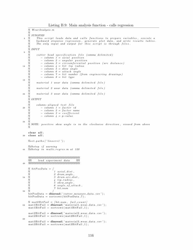
Listing B.9: Main analysis function - calls regression% WearAnalysis .m%% SYNOPSIS
4 % This s c r i p t l oads data and c a l l s f unc t i on s to prepare va r i a b l e s , execute a% backward s t epw i s e regres s ion , generate p l o t data , and wr i t e r e s u l t s t a b l e s .% The only input and output f o r t h i s s c r i p t i s through f i l e s .%% INPUT
9 %% cu t t e r head s p e c i f i c a t i o n f i l e (comma de l im i t ed )% − column 1 = ax i a l p o s i t i on% − column 2 = angular po s i t i on% − column 3 = c i r cumf e r en t i a l p o s i t i on ( arc d i s t ance )
14 % − column 4 = b i t t i p rad ius% − column 5 = skew ang le% − column 6 = at tack ang le% − column 7 = b i t number ( from eng ineer ing drawings )% − column 8 = b i t type
19 %% mater ia l 1 wear data (comma de l im i t ed f i l e )%% mater ia l 2 wear data (comma de l im i t ed f i l e )%
24 % mater ia l 3 wear data (comma de l im i t ed f i l e )%% OUTPUT%% column−a l i gned t e x t f i l e
29 % − column 1 = fa c t o r id% − column 2 = fa c t o r name% − column 3 = c o e f f i c i e n t% − column 4 = p−va lue%
34 %% NOTE: p o s i t i v e skew ang le i s in the c l o ckw i s e d i r e c t i on , viewed from above%
clear a l l ;39 close a l l ;
%se t p a t h s ( ’ l i n s e r v1 ’ ) ;
%dbstop i f warning44 %dbstop in mu l t i r e g r e s .m at 120
%%%%%%%%%%%%%%%%%%%%%%%%%%%%%%%%%% load experiment data %%
49 %%%%%%%%%%%%%%%%%%%%%%%%%%%%%%%%
% bitPosData = [% 1 a x i a l d i s t ,% 2 drum angle ,
54 % 3 drum arc dis t ,% 4 t i p r ad i u s ,% 5 skew angle ,% 6 ang l e o f a t t a c k ,% 7 bit num
59 % ]bitPosData = dlmread( ’ cut te r measure data . csv ’ ) ;bitPosData = sort rows ( bitPosData , 7 ) ;
% mat0BitFai l = [ bit num , f a i l c o u n t ]64 mat1BitFai l = dlmread( ’ mate r i a l 1 wear data . csv ’ ) ;
mat1BitFai l = sor t rows ( mat1BitFail , 1 ) ;
mat2BitFai l = dlmread( ’ mate r i a l 2 wear data . csv ’ ) ;mat2BitFai l = sor t rows ( mat2BitFail , 1 ) ;
69
mat3BitFai l = dlmread( ’ mate r i a l 3 wear data . csv ’ ) ;mat3BitFai l = sor t rows ( mat3BitFail , 1 ) ;
116
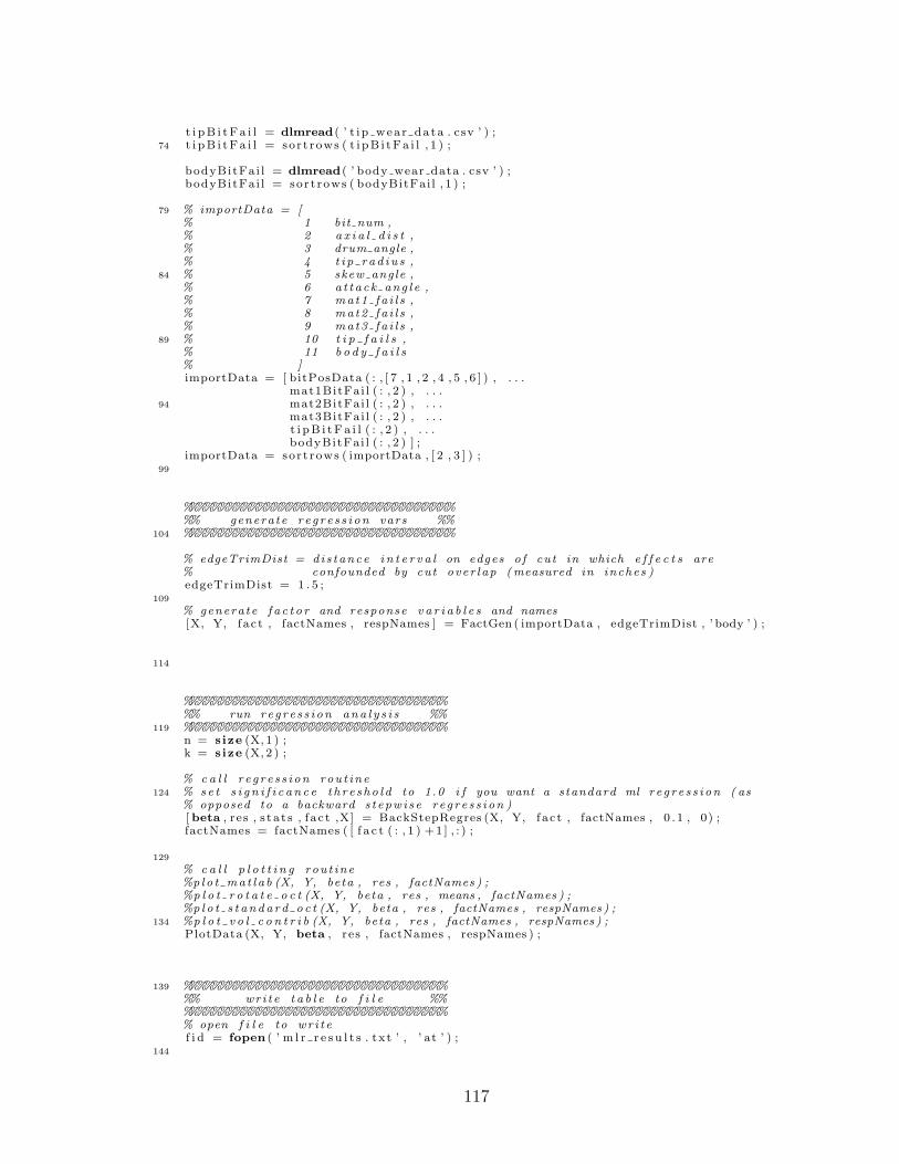
t i pB i tFa i l = dlmread( ’ t i p wear data . csv ’ ) ;74 t i pB i tFa i l = sor t rows ( t i pB i tFa i l , 1 ) ;
bodyBitFai l = dlmread( ’ body wear data . csv ’ ) ;bodyBitFai l = sor t rows ( bodyBitFai l , 1 ) ;
79 % importData = [% 1 bit num ,% 2 a x i a l d i s t ,% 3 drum angle ,% 4 t i p r ad i u s ,
84 % 5 skew angle ,% 6 a t t ack ang l e ,% 7 mat1 fa i l s ,% 8 mat2 fa i l s ,% 9 mat3 fa i l s ,
89 % 10 t i p f a i l s ,% 11 b o d y f a i l s% ]importData = [ bitPosData ( : , [ 7 , 1 , 2 , 4 , 5 , 6 ] ) , . . .
mat1BitFai l ( : , 2 ) , . . .94 mat2BitFai l ( : , 2 ) , . . .
mat3BitFai l ( : , 2 ) , . . .t i pB i tF a i l ( : , 2 ) , . . .bodyBitFai l ( : , 2 ) ] ;
importData = sort rows ( importData , [ 2 , 3 ] ) ;99
%%%%%%%%%%%%%%%%%%%%%%%%%%%%%%%%%%%%%% generate r e g r e s s i on vars %%
104 %%%%%%%%%%%%%%%%%%%%%%%%%%%%%%%%%%%%
% edgeTrimDist = d i s tance i n t e r v a l on edges o f cut in which e f f e c t s are% confounded by cut over lap (measured in inches )edgeTrimDist = 1 . 5 ;
109
% generate f a c t o r and response v a r i a b l e s and names[X, Y, fac t , factNames , respNames ] = FactGen ( importData , edgeTrimDist , ’ body ’ ) ;
114
%%%%%%%%%%%%%%%%%%%%%%%%%%%%%%%%%%%%% run reg r e s s i on ana l y s i s %%
119 %%%%%%%%%%%%%%%%%%%%%%%%%%%%%%%%%%%n = s ize (X, 1 ) ;k = s ize (X, 2 ) ;
% c a l l r e g r e s s i on rou t ine124 % se t s i g n i f i c a n c e t h r e s ho l d to 1.0 i f you want a standard ml r e g r e s s i on ( as
% opposed to a backward s t epw i s e r e g r e s s i on )[ beta , res , s t a t s , f ac t ,X] = BackStepRegres (X, Y, fac t , factNames , 0 . 1 , 0) ;factNames = factNames ( [ f a c t ( : , 1 ) +1 ] , : ) ;
129
% c a l l p l o t t i n g rou t ine%p lo t ma t l a b (X, Y, beta , res , factNames ) ;%p l o t r o t a t e o c t (X, Y, beta , res , means , factNames ) ;%p l o t s t anda r d o c t (X, Y, beta , res , factNames , respNames ) ;
134 %p l o t v o l c o n t r i b (X, Y, beta , res , factNames , respNames ) ;PlotData (X, Y, beta , res , factNames , respNames ) ;
139 %%%%%%%%%%%%%%%%%%%%%%%%%%%%%%%%%%%%% wri t e t a b l e to f i l e %%%%%%%%%%%%%%%%%%%%%%%%%%%%%%%%%%%%%% open f i l e to wr i t ef i d = fopen ( ’ m l r r e s u l t s . txt ’ , ’ at ’ ) ;
144
117

% pr in t r e g r e s s i on repor t headerheadFormat = ’%−6s \ t%−26s \ t%8s \ t%7s \n ’ ;bodyFormat = ’%−6s \ t%−26s \ t%8.4 f \ t%6.4 f \n ’ ;
149 p r i n t f ( ’ \n%s \n ’ , respNames {1 ,3} ) ;fpr intf ( f i d , ’ \n%s \n ’ , respNames {1 ,3} ) ;p r i n t f ( headFormat , ’ f a c t o r ’ , ’ d e s c r i p t i o n ’ , ’ c o e f f ’ , ’p−value ’ ) ;fpr intf ( f i d , headFormat , ’ f a c t o r ’ , ’ d e s c r i p t i o n ’ , ’ c o e f f ’ , ’p−value ’ ) ;
154 % pr in t f a c t o r datafor i = 1 : s ize (X, 2 )
p r i n t f ( bodyFormat , factNames{ i , 2} , factNames{ i , 3} , beta ( i , 1 ) , beta ( i , 3 ) ) ;fpr intf ( f i d , bodyFormat , factNames{ i , 2} , factNames{ i , 3} , beta ( i , 1 ) ,beta ( i , 3 ) ) ;
end159
p r i n t f ( ’ \n ’ ) ;fpr intf ( f i d , ’ \n ’ ) ;p r i n t f ( ’%s \n ’ , [ ’R−Square = ’ , num2str( s t a t s (1 ) ) ] ) ;fpr intf ( f i d , ’%s \n ’ , [ ’R−Square = ’ , num2str( s t a t s (1 ) ) ] ) ;
164 p r i n t f ( ’%s \n ’ , [ ’ Adjusted R−Square = ’ , num2str( s t a t s (2 ) ) ] ) ;fpr intf ( f i d , ’%s \n ’ , [ ’ Adjusted R−Square = ’ , num2str( s t a t s (2 ) ) ] ) ;p r i n t f ( ’ \n ’ ) ;
fc lose ( f i d ) ;
118

Listing B.10: Generate regression variables and related information% FactGen .m
2 %% SYNOPSIS% This func t i on accep t s fundamental data from a s p e c i f i c c u t t i n g app l i ca t i on ,% and re turns r e g r e s s i on v a r i a b l e s and r e l a t e d information , f o r the s p e c i f i e d% f a i l u r e mode .
7 %% INPUT%% funData : fundamental data from a s p e c i f i c c u t t i n g app l i c a t i on% column 1 = bit num ,
12 % column 2 = a x i a l d i s t ,% column 3 = drum angle ,% column 4 = t i p r ad i u s ,% column 5 = skew angle ,% column 6 = at tack ang l e ,
17 % column 7 = mat1 fa i l s ,% column 8 = mat2 fa i l s ,% column 9 = mat3 fa i l s ,% column 10 = t i p f a i l s ,% column 11 = b o d y f a i l s
22 %% edgeTrimDist : d i s t ance i n t e r v a l on edges o f cut in which e f f e c t s are% confounded by cut over lap (measured in inches ) . These b i t s% are removed from the ana l y s i s%
27 % mode : f a i l u r e mode s t r ing , c on i s t i n g o f one o f the f o l l ow i n g :% ’ body ’ = body f a i l u r e mode% ’ t ip ’ = t i p f a i l u r e mode%% OUTPUT
32 %% Y: vec tor conta in ing va lue s f o r the dependent or response v a r i a b l e%% X: matrix o f independent v a r i a b l e va lue s ( rows=samples , columns=f a c t o r s )%
37 % fa c t : indexed l i s t o f f a c t o r i n t e r a c t i o n s (number o f rows shou ld equa l% number o f columns in X)% column 1 = fa c t o r number% column 2 = in t e r a c t i on f a c t o r 1 (0 fo r l i n e a r terms )% column 3 = in t e r a c t i on f a c t o r 2 (0 fo r l i n e a r terms )
42 %% factNames : names o f f a c t o r s f o r r epor t ing purposes ( c e l l array )% column 1 = va r i a b l e index% column 2 = va r i a b l e id% column 3 = va r i a b l e name
47 %% example c e l l array : f a c t o r names% −−−−−−−−−−−−−−−−−−−−−−−−−−−−−−−−−−−−−−−−−−−−−−−−% index | v a r i a b l e i d | var iab le name% −−−−−−−+−−−−−−−−−−−−−−−+−−−−−−−−−−−−−−−−−−−−−−−−
52 % 1 | X01 | drum angle% 2 | X02 | t i p r a d i u s% 3 | X03 | skew ang le% 4 | X01X02 | drum angle X t i p r a d i u s% 5 | X01X03 | drum angle X skew ang le
57 % 6 | X02X03 | t i p r a d i u s X skew ang le% −−−−−−−−−−−−−−−−−−−−−−−−−−−−−−−−−−−−−−−−−−−−−−−−% factNames (1 ,1 :3 ) = [{1} ,{ ’X01 ’} ,{ ’ drum angle ’ } ] ;%% respNames : name of response v a r i a b l e
62 % column 1 = va r i a b l e index% column 2 = va r i a b l e id% column 3 = va r i a b l e name%
67 function [X,Y, fac t , factNames , respNames ] = FactGen ( funData , edgeTrimDist , mode) ;
119
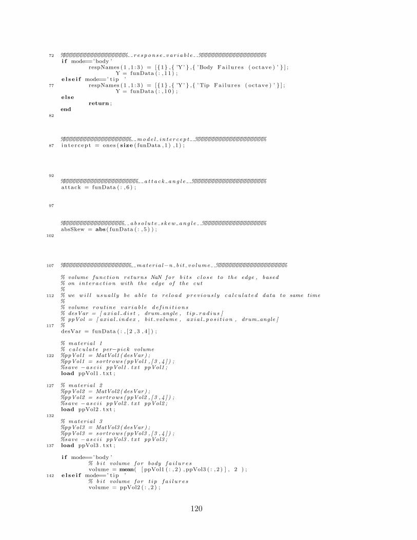
72 %%%%%%%%%%%%%%%%%%% re s p on s e v a r i a b l e %%%%%%%%%%%%%%%%%%%i f mode==’ body ’
respNames ( 1 , 1 : 3 ) = [{1} ,{ ’Y ’ } ,{ ’Body Fa i l u r e s ( octave ) ’ } ] ;Y = funData ( : , 1 1 ) ;
e l s e i f mode==’ t i p ’77 respNames ( 1 , 1 : 3 ) = [{1} ,{ ’Y ’ } ,{ ’ Tip Fa i l u r e s ( octave ) ’ } ] ;
Y = funData ( : , 1 0 ) ;else
return ;end
82
%%%%%%%%%%%%%%%%%%%% mode l i n t e r c e p t %%%%%%%%%%%%%%%%%%%%87 i n t e r c e p t = ones ( s ize ( funData , 1 ) ,1 ) ;
92
%%%%%%%%%%%%%%%%%%%%%% a t t a c k a n g l e %%%%%%%%%%%%%%%%%%%%%attack = funData ( : , 6 ) ;
97
%%%%%%%%%%%%%%%%%% ab s o l u t e s k ew an g l e %%%%%%%%%%%%%%%%%%absSkew = abs ( funData ( : , 5 ) ) ;
102
107 %%%%%%%%%%%%%%%%%%%% mater ia l−n b i t v o l ume %%%%%%%%%%%%%%%%%%%%
% volume func t ion re turns NaN for b i t s c l o s e to the edge , based% on in t e r a c t i on with the edge o f the cut%
112 % we w i l l u s ua l l y be ab l e to re load p r e v i ou s l y c a l c u l a t e d data to same time%% volume rou t ine v a r i a b l e d e f i n i t i o n s% desVar = [ a x i a l d i s t , drum angle , t i p r a d i u s ]% ppVol = [ ax i a l i nde x , b i t vo lume , a x i a l p o s i t i o n , drum angle ]
117 %desVar = funData ( : , [ 2 , 3 , 4 ] ) ;
% mater ia l 1% ca l c u l a t e per−p ick volume
122 %ppVol1 = MatVol1 ( desVar ) ;%ppVol1 = sortrows ( ppVol1 , [ 3 , 4 ] ) ;%save −a s c i i ppVol1 . t x t ppVol1 ;load ppVol1 . txt ;
127 % mater ia l 2%ppVol2 = MatVol2 ( desVar ) ;%ppVol2 = sortrows ( ppVol2 , [ 3 , 4 ] ) ;%save −a s c i i ppVol2 . t x t ppVol2 ;load ppVol2 . txt ;
132
% mater ia l 3%ppVol3 = MatVol3 ( desVar ) ;%ppVol3 = sortrows ( ppVol3 , [ 3 , 4 ] ) ;%save −a s c i i ppVol3 . t x t ppVol3 ;
137 load ppVol3 . txt ;
i f mode==’ body ’% b i t volume fo r body f a i l u r e svolume = mean( [ ppVol1 ( : , 2 ) , ppVol3 ( : , 2 ) ] , 2 ) ;
142 e l s e i f mode==’ t i p ’% b i t volume fo r t i p f a i l u r e svolume = ppVol2 ( : , 2 ) ;
120
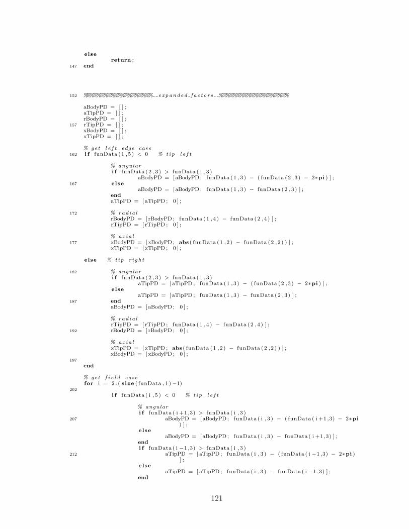
elsereturn ;
147 end
152 %%%%%%%%%%%%%%%%%%%% expanded f a c t o r s %%%%%%%%%%%%%%%%%%%%
aBodyPD = [ ] ;aTipPD = [ ] ;rBodyPD = [ ] ;
157 rTipPD = [ ] ;xBodyPD = [ ] ;xTipPD = [ ] ;
% get l e f t edge case162 i f funData (1 , 5 ) < 0 % t i p l e f t
% angulari f funData (2 , 3 ) > funData (1 , 3 )
aBodyPD = [ aBodyPD ; funData (1 , 3 ) − ( funData (2 , 3 ) − 2∗pi ) ] ;167 else
aBodyPD = [ aBodyPD ; funData (1 , 3 ) − funData (2 , 3 ) ] ;endaTipPD = [ aTipPD ; 0 ] ;
172 % rad i a lrBodyPD = [ rBodyPD ; funData (1 , 4 ) − funData (2 , 4 ) ] ;rTipPD = [ rTipPD ; 0 ] ;
% ax i a l177 xBodyPD = [xBodyPD ; abs ( funData (1 , 2 ) − funData (2 , 2 ) ) ] ;
xTipPD = [ xTipPD ; 0 ] ;
else % t i p r i g h t
182 % angulari f funData (2 , 3 ) > funData (1 , 3 )
aTipPD = [ aTipPD ; funData (1 , 3 ) − ( funData (2 , 3 ) − 2∗pi ) ] ;else
aTipPD = [ aTipPD ; funData (1 , 3 ) − funData (2 , 3 ) ] ;187 end
aBodyPD = [ aBodyPD ; 0 ] ;
% rad i a lrTipPD = [ rTipPD ; funData (1 , 4 ) − funData (2 , 4 ) ] ;
192 rBodyPD = [ rBodyPD ; 0 ] ;
% ax i a lxTipPD = [ xTipPD ; abs ( funData (1 , 2 ) − funData (2 , 2 ) ) ] ;xBodyPD = [xBodyPD ; 0 ] ;
197
end
% get f i e l d casefor i = 2 : ( s ize ( funData , 1 ) −1)
202
i f funData ( i , 5 ) < 0 % t i p l e f t
% angulari f funData ( i +1 ,3) > funData ( i , 3 )
207 aBodyPD = [ aBodyPD ; funData ( i , 3 ) − ( funData ( i +1 ,3) − 2∗pi) ] ;
elseaBodyPD = [ aBodyPD ; funData ( i , 3 ) − funData ( i +1 ,3) ] ;
endi f funData ( i −1 ,3) > funData ( i , 3 )
212 aTipPD = [ aTipPD ; funData ( i , 3 ) − ( funData ( i −1 ,3) − 2∗pi )] ;
elseaTipPD = [ aTipPD ; funData ( i , 3 ) − funData ( i −1 ,3) ] ;
end
121

217 % rad i a lrBodyPD = [ rBodyPD ; funData ( i , 4 ) − funData ( i +1 ,4) ] ;rTipPD = [ rTipPD ; funData ( i , 4 ) − funData ( i −1 ,4) ] ;
% ax i a l222 xBodyPD = [xBodyPD ; abs ( funData ( i , 2 ) − funData ( i +1 ,2) ) ] ;
xTipPD = [ xTipPD ; abs ( funData ( i , 2 ) − funData ( i −1 ,2) ) ] ;
else % t i p r i g h t
227 % angulari f funData ( i +1 ,3) > funData ( i , 3 )
aTipPD = [ aTipPD ; funData ( i , 3 ) − ( funData ( i +1 ,3) − 2∗pi )] ;
elseaTipPD = [ aTipPD ; funData ( i , 3 ) − funData ( i +1 ,3) ] ;
232 endi f funData ( i −1 ,3) > funData ( i , 3 )
aBodyPD = [ aBodyPD ; funData ( i , 3 ) − ( funData ( i −1 ,3) − 2∗pi) ] ;
elseaBodyPD = [ aBodyPD ; funData ( i , 3 ) − funData ( i −1 ,3) ] ;
237 end
% rad i a lrTipPD = [ rTipPD ; funData ( i , 4 ) − funData ( i +1 ,4) ] ;rBodyPD = [ rBodyPD ; funData ( i , 4 ) − funData ( i −1 ,4) ] ;
242
% ax i a lxTipPD = [ xTipPD ; abs ( funData ( i , 2 ) − funData ( i +1 ,2) ) ] ;xBodyPD = [xBodyPD ; abs ( funData ( i , 2 ) − funData ( i −1 ,2) ) ] ;
247 end
end
% get r i g h t edge case252 i f funData (1 , 5 ) > 0 % t i p r i g h t
% angulari f funData (end−1 ,3) > funData (end , 3 )
aBodyPD = [ aBodyPD ; funData (end , 3 ) − ( funData (end−1 ,3) − 2∗pi ) ] ;257 else
aBodyPD = [ aBodyPD ; funData (end , 3 ) − funData (end−1 ,3) ] ;endaTipPD = [ aTipPD ; 0 ] ;
262 % rad i a lrBodyPD = [ rBodyPD ; funData (end , 4 ) − funData (end−1 ,4) ] ;rTipPD = [ rTipPD ; 0 ] ;
% ax i a l267 xBodyPD = [xBodyPD ; abs ( funData (end , 2 ) − funData (end−1 ,2) ) ] ;
xTipPD = [ xTipPD ; 0 ] ;
else % t i p l e f t
272 % angulari f funData (end−1 ,3) > funData (end , 3 )
aTipPD = [ aTipPD ; funData (end , 3 ) − ( funData (end−1 ,3) − 2∗pi ) ] ;else
aTipPD = [ aTipPD ; funData (end , 3 ) − funData (end−1 ,3) ] ;277 end
aBodyPD = [ aBodyPD ; 0 ] ;
% rad i a lrTipPD = [ rTipPD ; funData (end , 4 ) − funData (end−1 ,4) ] ;
282 rBodyPD = [ rBodyPD ; 0 ] ;
% ax i a lxTipPD = [ xTipPD ; abs ( funData (end , 2 ) − funData (end−1 ,2) ) ] ;xBodyPD = [xBodyPD ; 0 ] ;
122

287
end
292
%%%%%%%%%%%%%%%%%%%% as s i g n o u t p u t %%%%%%%%%%%%%%%%%%%%X = [ ] ;f a c t = [ ] ;
297
% main f a c t o r sfactNames ( 1 , 1 : 3 ) = [{0} ,{ ’X00 ’ } ,{ ’ i n t e r c e p t ’ } ] ;
X = [X, i n t e r c e p t ] ;f a c t = [ f a c t ; [ 0 , 0 , 0 ] ] ;
302 factNames ( 2 , 1 : 3 ) = [{1} ,{ ’X01 ’ } ,{ ’ a t tack ’ } ] ;X = [X, attack ] ;f a c t = [ f a c t ; [ 1 , 0 , 0 ] ] ;
factNames ( 3 , 1 : 3 ) = [{2} ,{ ’X02 ’ } ,{ ’ absSkew ’ } ] ;X = [X, absSkew ] ;
307 f a c t = [ f a c t ; [ 2 , 0 , 0 ] ] ;factNames ( 4 , 1 : 3 ) = [{3} ,{ ’X03 ’ } ,{ ’ volume ’ } ] ;
X = [X, volume ] ;f a c t = [ f a c t ; [ 3 , 0 , 0 ] ] ;
factNames ( 5 , 1 : 3 ) = [{4} ,{ ’X04 ’ } ,{ ’xBodyPD ’ } ] ;312 X = [X, xBodyPD ] ;
f a c t = [ f a c t ; [ 4 , 0 , 0 ] ] ;factNames ( 6 , 1 : 3 ) = [{5} ,{ ’X05 ’ } ,{ ’xTipPD ’ } ] ;
X = [X, xTipPD ] ;f a c t = [ f a c t ; [ 5 , 0 , 0 ] ] ;
317 factNames ( 7 , 1 : 3 ) = [{6} ,{ ’X06 ’ } ,{ ’ rBodyPD ’ } ] ;X = [X, rBodyPD ] ;f a c t = [ f a c t ; [ 6 , 0 , 0 ] ] ;
factNames ( 8 , 1 : 3 ) = [{7} ,{ ’X07 ’ } ,{ ’ rTipPD ’ } ] ;X = [X, rTipPD ] ;
322 f a c t = [ f a c t ; [ 7 , 0 , 0 ] ] ;factNames ( 9 , 1 : 3 ) = [{8} ,{ ’X08 ’ } ,{ ’aBodyPD ’ } ] ;
X = [X, aBodyPD ] ;f a c t = [ f a c t ; [ 8 , 0 , 0 ] ] ;
factNames ( 1 0 , 1 : 3 ) = [{9} ,{ ’X09 ’ } ,{ ’ aTipPD ’ } ] ;327 X = [X, aTipPD ] ;
f a c t = [ f a c t ; [ 9 , 0 , 0 ] ] ;
% tr im and sca l e da ta[X, Y] = EdgeTrim (X, Y, funData , edgeTrimDist ) ;
332 %for i = 2: s i z e (X,2 )% X( : , i ) = (X( : , i )−((max(X( : , i ) )+min(X( : , i ) ) ) /2) ) /((max(X( : , i ) )−min(X( : , i ) ) ) /2) ;%end
% in t e r a c t i on f a c t o r s337 factNames ( 1 1 , 1 : 3 ) = [{10} ,{ ’X10 ’ } ,{ ’ a t tack x absSkew ’ } ] ;
X = [X, X( : , 2 ) .∗ X( : , 3 ) ] ;f a c t = [ f a c t ; [ 1 0 , 1 , 2 ] ] ;
factNames ( 1 2 , 1 : 3 ) = [{11} ,{ ’X11 ’ } ,{ ’ a t tack x volume ’ } ] ;X = [X, X( : , 2 ) .∗ X( : , 4 ) ] ;
342 f a c t = [ f a c t ; [ 1 1 , 1 , 3 ] ] ;factNames ( 1 3 , 1 : 3 ) = [{12} ,{ ’X12 ’ } ,{ ’ a t tack x xBodyPD ’ } ] ;
X = [X, X( : , 2 ) .∗ X( : , 5 ) ] ;f a c t = [ f a c t ; [ 1 2 , 1 , 4 ] ] ;
factNames ( 1 4 , 1 : 3 ) = [{13} ,{ ’X13 ’ } ,{ ’ a t tack x xTipPD ’ } ] ;347 X = [X, X( : , 2 ) .∗ X( : , 6 ) ] ;
f a c t = [ f a c t ; [ 1 3 , 1 , 5 ] ] ;factNames ( 1 5 , 1 : 3 ) = [{14} ,{ ’X14 ’ } ,{ ’ a t tack x rBodyPD ’ } ] ;
X = [X, X( : , 2 ) .∗ X( : , 7 ) ] ;f a c t = [ f a c t ; [ 1 4 , 1 , 6 ] ] ;
352 factNames ( 1 6 , 1 : 3 ) = [{15} ,{ ’X15 ’ } ,{ ’ a t tack x rTipPD ’ } ] ;X = [X, X( : , 2 ) .∗ X( : , 8 ) ] ;f a c t = [ f a c t ; [ 1 5 , 1 , 7 ] ] ;
factNames ( 1 7 , 1 : 3 ) = [{16} ,{ ’X16 ’ } ,{ ’ a t tack x aBodyPD ’ } ] ;X = [X, X( : , 2 ) .∗ X( : , 9 ) ] ;
357 f a c t = [ f a c t ; [ 1 6 , 1 , 8 ] ] ;factNames ( 1 8 , 1 : 3 ) = [{17} ,{ ’X17 ’ } ,{ ’ a t tack x aTipPD ’ } ] ;
X = [X, X( : , 2 ) .∗ X( : , 1 0 ) ] ;
123

f a c t = [ f a c t ; [ 1 7 , 1 , 9 ] ] ;factNames ( 1 9 , 1 : 3 ) = [{18} ,{ ’X18 ’ } ,{ ’ absSkew x volume ’ } ] ;
362 X = [X, X( : , 3 ) .∗ X( : , 4 ) ] ;f a c t = [ f a c t ; [ 1 8 , 2 , 3 ] ] ;
factNames ( 2 0 , 1 : 3 ) = [{19} ,{ ’X19 ’ } ,{ ’ absSkew x xBodyPD ’ } ] ;X = [X, X( : , 3 ) .∗ X( : , 5 ) ] ;f a c t = [ f a c t ; [ 1 9 , 2 , 4 ] ] ;
367 factNames ( 2 1 , 1 : 3 ) = [{20} ,{ ’X20 ’ } ,{ ’ absSkew x xTipPD ’ } ] ;X = [X, X( : , 3 ) .∗ X( : , 6 ) ] ;f a c t = [ f a c t ; [ 2 0 , 2 , 5 ] ] ;
factNames ( 2 2 , 1 : 3 ) = [{21} ,{ ’X21 ’ } ,{ ’ absSkew x rBodyPD ’ } ] ;X = [X, X( : , 3 ) .∗ X( : , 7 ) ] ;
372 f a c t = [ f a c t ; [ 2 1 , 2 , 6 ] ] ;factNames ( 2 3 , 1 : 3 ) = [{22} ,{ ’X22 ’ } ,{ ’ absSkew x rTipPD ’ } ] ;
X = [X, X( : , 3 ) .∗ X( : , 8 ) ] ;f a c t = [ f a c t ; [ 2 2 , 2 , 7 ] ] ;
factNames ( 2 4 , 1 : 3 ) = [{23} ,{ ’X23 ’ } ,{ ’ absSkew x aBodyPD ’ } ] ;377 X = [X, X( : , 3 ) .∗ X( : , 9 ) ] ;
f a c t = [ f a c t ; [ 2 3 , 2 , 8 ] ] ;factNames ( 2 5 , 1 : 3 ) = [{24} ,{ ’X24 ’ } ,{ ’ absSkew x aTipPD ’ } ] ;
X = [X, X( : , 3 ) .∗ X( : , 1 0 ) ] ;f a c t = [ f a c t ; [ 2 4 , 2 , 9 ] ] ;
382 factNames ( 2 6 , 1 : 3 ) = [{25} ,{ ’X25 ’ } ,{ ’ volume x xBodyPD ’ } ] ;X = [X, X( : , 4 ) .∗ X( : , 5 ) ] ;f a c t = [ f a c t ; [ 2 5 , 3 , 4 ] ] ;
factNames ( 2 7 , 1 : 3 ) = [{26} ,{ ’X26 ’ } ,{ ’ volume x xTipPD ’ } ] ;X = [X, X( : , 4 ) .∗ X( : , 6 ) ] ;
387 f a c t = [ f a c t ; [ 2 6 , 3 , 5 ] ] ;factNames ( 2 8 , 1 : 3 ) = [{27} ,{ ’X27 ’ } ,{ ’ volume x rBodyPD ’ } ] ;
X = [X, X( : , 4 ) .∗ X( : , 7 ) ] ;f a c t = [ f a c t ; [ 2 7 , 3 , 6 ] ] ;
factNames ( 2 9 , 1 : 3 ) = [{28} ,{ ’X28 ’ } ,{ ’ volume x rTipPD ’ } ] ;392 X = [X, X( : , 4 ) .∗ X( : , 8 ) ] ;
f a c t = [ f a c t ; [ 2 8 , 3 , 7 ] ] ;factNames ( 3 0 , 1 : 3 ) = [{29} ,{ ’X29 ’ } ,{ ’ volume x aBodyPD ’ } ] ;
X = [X, X( : , 4 ) .∗ X( : , 9 ) ] ;f a c t = [ f a c t ; [ 2 9 , 3 , 8 ] ] ;
397 factNames ( 3 1 , 1 : 3 ) = [{30} ,{ ’X30 ’ } ,{ ’ volume x aTipPD ’ } ] ;X = [X, X( : , 4 ) .∗ X( : , 1 0 ) ] ;f a c t = [ f a c t ; [ 3 0 , 3 , 9 ] ] ;
factNames ( 3 2 , 1 : 3 ) = [{31} ,{ ’X31 ’ } ,{ ’xBodyPD x xTipPD ’ } ] ;X = [X, X( : , 5 ) .∗ X( : , 6 ) ] ;
402 f a c t = [ f a c t ; [ 3 1 , 4 , 5 ] ] ;factNames ( 3 3 , 1 : 3 ) = [{32} ,{ ’X32 ’ } ,{ ’xBodyPD x rBodyPD ’ } ] ;
X = [X, X( : , 5 ) .∗ X( : , 7 ) ] ;f a c t = [ f a c t ; [ 3 2 , 4 , 6 ] ] ;
factNames ( 3 4 , 1 : 3 ) = [{33} ,{ ’X33 ’ } ,{ ’xBodyPD x rTipPD ’ } ] ;407 X = [X, X( : , 5 ) .∗ X( : , 8 ) ] ;
f a c t = [ f a c t ; [ 3 3 , 4 , 7 ] ] ;factNames ( 3 5 , 1 : 3 ) = [{34} ,{ ’X34 ’ } ,{ ’xBodyPD x aBodyPD ’ } ] ;
X = [X, X( : , 5 ) .∗ X( : , 9 ) ] ;f a c t = [ f a c t ; [ 3 4 , 4 , 8 ] ] ;
412 factNames ( 3 6 , 1 : 3 ) = [{35} ,{ ’X35 ’ } ,{ ’xBodyPD x aTipPD ’ } ] ;X = [X, X( : , 5 ) .∗ X( : , 1 0 ) ] ;f a c t = [ f a c t ; [ 3 5 , 4 , 9 ] ] ;
factNames ( 3 7 , 1 : 3 ) = [{36} ,{ ’X36 ’ } ,{ ’xTipPD x rBodyPD ’ } ] ;X = [X, X( : , 6 ) .∗ X( : , 7 ) ] ;
417 f a c t = [ f a c t ; [ 3 6 , 5 , 6 ] ] ;factNames ( 3 8 , 1 : 3 ) = [{37} ,{ ’X37 ’ } ,{ ’xTipPD x rTipPD ’ } ] ;
X = [X, X( : , 6 ) .∗ X( : , 8 ) ] ;f a c t = [ f a c t ; [ 3 7 , 5 , 7 ] ] ;
factNames ( 3 9 , 1 : 3 ) = [{38} ,{ ’X38 ’ } ,{ ’xTipPD x aBodyPD ’ } ] ;422 X = [X, X( : , 6 ) .∗ X( : , 9 ) ] ;
f a c t = [ f a c t ; [ 3 8 , 5 , 8 ] ] ;factNames ( 4 0 , 1 : 3 ) = [{39} ,{ ’X39 ’ } ,{ ’xTipPD x aTipPD ’ } ] ;
X = [X, X( : , 6 ) .∗ X( : , 1 0 ) ] ;f a c t = [ f a c t ; [ 3 9 , 5 , 9 ] ] ;
427 factNames ( 4 1 , 1 : 3 ) = [{40} ,{ ’X40 ’ } ,{ ’ rBodyPD x rTipPD ’ } ] ;X = [X, X( : , 7 ) .∗ X( : , 8 ) ] ;f a c t = [ f a c t ; [ 4 0 , 6 , 7 ] ] ;
factNames ( 4 2 , 1 : 3 ) = [{41} ,{ ’X41 ’ } ,{ ’ rBodyPD x aBodyPD ’ } ] ;X = [X, X( : , 7 ) .∗ X( : , 9 ) ] ;
432 f a c t = [ f a c t ; [ 4 1 , 6 , 8 ] ] ;
124

factNames ( 4 3 , 1 : 3 ) = [{42} ,{ ’X42 ’ } ,{ ’ rBodyPD x aTipPD ’ } ] ;X = [X, X( : , 7 ) .∗ X( : , 1 0 ) ] ;f a c t = [ f a c t ; [ 4 2 , 6 , 9 ] ] ;
factNames ( 4 4 , 1 : 3 ) = [{43} ,{ ’X43 ’ } ,{ ’ rTipPD x aBodyPD ’ } ] ;437 X = [X, X( : , 8 ) .∗ X( : , 9 ) ] ;
f a c t = [ f a c t ; [ 4 3 , 7 , 8 ] ] ;factNames ( 4 5 , 1 : 3 ) = [{44} ,{ ’X44 ’ } ,{ ’ rTipPD x aTipPD ’ } ] ;
X = [X, X( : , 8 ) .∗ X( : , 1 0 ) ] ;f a c t = [ f a c t ; [ 4 4 , 7 , 9 ] ] ;
442 factNames ( 4 6 , 1 : 3 ) = [{45} ,{ ’X45 ’ } ,{ ’aBodyPD x aTipPD ’ } ] ;X = [X, X( : , 9 ) .∗ X( : , 1 0 ) ] ;f a c t = [ f a c t ; [ 4 5 , 8 , 9 ] ] ;
447
return ;
125

Listing B.11: Trim bit data, removing confounding edge effects% EdgeTrim .m
2 %% SYNOPSIS% This func t i on modi f i e s the X and Y matr ices by removing data r e l a t i n g to% b i t s l o ca t ed wi th in a ce r t a in d i s t ance o f the edge o f the cut . Candidate% b i t s are i d e n t i f i e d us ing fundamental measured data .
7 %% INPUT%% X: matrix o f independent v a r i a b l e va lue s ( rows=samples , columns=f a c t o r s )%
12 % Y: vec tor conta in ing va lue s f o r the dependent or response v a r i a b l e%% funData : fundamental data from a s p e c i f i c c u t t i n g app l i c a t i on% column 1 = bit num ,% column 2 = a x i a l d i s t ,
17 % column 3 = drum angle ,% column 4 = t i p r ad i u s ,% column 5 = skew angle ,% column 6 = at tack ang l e ,% column 7 = mat1 fa i l s ,
22 % column 8 = mat2 fa i l s ,% column 9 = mat3 fa i l s ,% column 10 = t i p f a i l s ,% column 11 = b o d y f a i l s%
27 % edgeTrimDist : d i s t ance i n t e r v a l on edges o f cut in which e f f e c t s are% confounded by cut over lap (measured in inches ) . These b i t s% are removed from the ana l y s i s%% OUTPUT
32 %% X trim : trimmed vers ion o f the X matrix%% Y trim : trimmed vers ion o f the Y matrix%
37
function [ X trim , Y trim ] = EdgeTrim(X, Y, funData , edgeTrimDist )
%%%%%%%%%%%%%%%%%%%%%%%%%%%%%%%%%%%%%%%%%%%%% remove edge over lap confounding %%
42 %%%%%%%%%%%%%%%%%%%%%%%%%%%%%%%%%%%%%%%%%%%X trim = X;Y trim = Y;
l e f tEdge = min( funData ( : , 2 ) ) ;47 r ightEdge = max( funData ( : , 2 ) ) ;
% trim l e f t confounded b i t swhile ( funData (1 , 2 ) < l e f tEdge + edgeTrimDist )
funData ( 1 , : ) = [ ] ;52 X trim ( 1 , : ) = [ ] ;
Y trim ( 1 , : ) = [ ] ;end
% trim r i g h t confounded b i t s57 while ( funData (end , 2 ) > r ightEdge − edgeTrimDist )
funData (end , : ) = [ ] ;X trim (end , : ) = [ ] ;Y trim (end , : ) = [ ] ;
end62
return ;
126

Listing B.12: Perform backward stepwise regression1 % BackStepRegres .m
%% SYNOPSIS% This func t i on performs a backward s t epw i s e r e g r e s s i on . I t i s cu r r en t l y% implemented to wr i t e a f i l e conta in ing a l a t e x t a b l e f o r each s t ep o f the
6 % regre s s i on .%%% INPUT%
11 % Y : vec tor conta in ing va lue s f o r the dependent or response v a r i a b l e%% X : matrix o f independent v a r i a b l e va lue s ( rows=samples , columns=f a c t o r s )%% fa c t : indexed l i s t o f f a c t o r i n t e r a c t i o n s (number o f rows shou ld equa l
16 % : number o f columns in X)% : column 1 −> f a c t o r number% : column 2 −> i n t e r a c t i on f a c t o r 1 (0 f o r l i n e a r terms )% : column 3 −> i n t e r a c t i on f a c t o r 2 (0 f o r l i n e a r terms )%
21 % factNames : names o f f a c t o r s f o r r epor t ing purposes ( c e l l array )% column 1 = va r i a b l e index% column 2 = va r i a b l e id% column 3 = va r i a b l e name%
26 % a : s i g n i f i c a n c e l e v e l ( t y p i c a l l y 0 .05)%% z : ( op t i ona l )% : z=0 −> f o r c e zero i n t e r c e p t ( or non−zero i n t e r c e p t inc luded in X)% : z=1 −> f i t non−zero i n t e r c e p t ( d e f a u l t )
31 %%% OUTPUT%% beta
36 % B hat : l e a s t squares c o e f f i c i e n t% T : t−s tuden t p r o b a b i l i t y f o r each c o e f f i c i e n t% P : p−va lue s f o r each c o e f f i c i e n t%% res
41 % Y hat : p r ed i c t ed response% E : r e s i d u a l s% Z : z−score o f r e s i d u a l s ( f o r normal p r o b a b i l i t y p l o t )% var Y hat : error in p red i c t ed response%
46 % s t a t s% R2 : propor t ion o f exp la ined va r i a t i on ( r−squared )% R2 adj : ad jus td r−squared% t s i g : 0.05 s i g n i f i c a n c e l e v e l f o r c o e f f i c i e n t s%
51 % means ( inc l ud ing i n t e r c e p t )% X mean : f a c t o r mean at each d i s c r e t e response l e v e l% Y mean : s e t o f d i s c r e t e response l e v e l s% Y hat mean : p r ed i c t i on at l e v e l mean% Y hat error : var iance in pred i c t ed response f o r means
56 %% trend% X trend : s e t o f appropr ia te x va lue s f o r each f a c t o r% Y trend : trend o f p r ed i c t ed response at X trend% Y error : standard dev in pred i c t ed response ( Y trend )
61 %%% IMPORTANT NOTE: To f i t an MLR model , the number o f% samples must be g r ea t e r than the number o f independent% va r i a b l e s . As the number o f v a r i a b l e s g e t s c l o s e r to
66 % the number o f samples , the X’X inve r s e matrix may become% uns tab l e and may not e x i s t ( i . e . , s i n gu l a r X’X matrix ) .%
71 function [ beta , res , s t a t s , f ac t ,X] = BackStepRegres (X,Y, fac t , factNames , a , z ) ;
127

% load octave func t i on wrappers f o r c ompa t i b i l i t y with matlab%path ( path , ’ / home/mht/ octave /wrappers ’ ) ;
76
% se t v a r i a b l e sf a c t i n = f a c t ;X in = X;
81 % check order o f i n t e r a c t i on f a c t o r sintOrder = s ize ( fac t , 2 ) −1;
% check fo r zero−i n t e r c ep t−f l a g86 i f nargin < 3
z=1;endi f z == 1
X = [ ones ( [ length (Y) , 1 ] ) , X ] ;91 f a c t = [ [ 0 , 0 , 0 ] ; f a c t ] ;
end
n = length (Y) ; % number o f samplesk = s ize (X, 2 ) ; % number o f f a c t o r s
96
% check to see t ha t n >= k ( samples >= independent vars )i f k>n
error ( ’More v a r i a b l e s than samples , ’ , . . .’ use l e s s v a r i a b l e s and/ or omit i n t e r c e p t ’ )
101 end
% maximum number o f i t e r a t i o n s equa l to number o f v a r i a b l e sstep num = 0 ;
106 while 1
k = s ize (X, 2 ) ; % number o f f a c t o r s
% c o e f f i c i e n t s and p r ed i c t i on s111 X ha l f i nv = inv (X’ ∗ X) ;
X inv = X ha l f i nv ∗ X’ ;B hat = X inv ∗ Y;Y hat = X ∗ B hat ;
116
% model c l o s ene s s (R−Squared , Adjusted R−Squared )SSE = (Y − X ∗ B hat ) ’ ∗ (Y − X ∗ B hat ) ;SST = sum( [ (Y − mean(Y) ) . ˆ 2 ] ) ;R2 = 1−SSE/SST ;
121 i f (0 )R2 adj = 1 − (1 − R2) ∗ ( ( n − 1) /(n − k − 1) ) ;
elseR2 adj = 1 − (1 − R2) ∗ ( ( n − 1) /(n − k ) ) ;
end126
% s t a t i s t i c a l s i g n i f i c a n c e o f c o e f f i c i e n t s (T−Value , P−Value )S2 = SSE/(n−k ) ;var B hat = diag ( X ha l f i nv ) ∗ S2 ;
131 s td B hat = var B hat . ˆ (1/2) ;T = B hat .∗ (1 . / std B hat ) ;t s i g = abs ( t inv ( 0 . 0 5/2 , ( n−k ) ) ) ;P = tcd f (−abs (T) , ( n−k ) ) ∗2 ;
136
% prec i s i on o f p r e d i c t i on svar Y hat = X ∗ X ha l f i nv ∗ X’ ∗ S2 ;
141 % check model assumptions ( r e s i dua l s , normal p r o b a b i l i t y )E = Y − Y hat ; % re s i d u a l sE ord = [E, [ 1 : n ] ’ ] ;E ord = [ [ 1 : n ] ’ , so r t rows ( E ord , 1 ) ] ; % re s i d u a l s ordered by s i z e
128

Z ord = norminv ( ( E ord ( : , 1 ) −0.5) / max( E ord ( : , 1 ) ) , 0 , 1 ) ;146 Z ord = [ E ord ( : , 3 ) , Z ord ] ; % Z−Score f o r E ord
Z = sort rows ( Z ord , 1 ) ;Z = Z ( : , 2 ) ; % Z−Score o f r e s i d u a l s in o r i g i n a l order
% arrange r e g r e s s i on r e s u l t s151 beta = [ B hat , T, P, var B hat ] ;
r e s = [ Y hat , E, Z ] ;s t a t s = [R2 , R2 adj , t s i g ] ;
% wri t e r e g r e s s i on r e s u l t s from t h i s s t ep to l a t e x t a bu l a r f i l e156 LatexTabMed( step num , fac t , factNames , s t a t s (1 ) , s t a t s (2 ) ,beta ( : , 3 ) ,beta ( : , 1 )
) ;
% f ind drop candidatefFact = [ fac t ,P, zeros ( s ize ( fac t , 1 ) , 1 ) ] ;
161 for j = 1 : s ize ( fac t , 1 )[ int , b ] = find ( fFact ( : , 2 : 3 )==fFact ( j , 1 ) ) ;i f length ( i n t )==0
fFact ( j , 5 ) = 1 ;end
166 end[ p , dFact ] = max( [ fFact ( : , 4 ) .∗ fFact ( : , 5 ) ] ) ;
% drop current f a c t o r from fa c t o r l i s t , f a c t o r names , and from X matrixi f fFact ( dFact , 4 ) > a
171 f a c t ( dFact , : ) = [ ] ;X( : , dFact ) = [ ] ;factNames ( dFact , : ) = [ ] ;
elsebreak
176 endstep num = step num + 1 ;
end
181 % wri t e f i n a l r e g r e s s i on r e s u l t s to l a t e x t a bu l a r f i l eLatexTabMed( step num , fac t , factNames , s t a t s (1 ) , s t a t s (2 ) ,beta ( : , 3 ) ,beta ( : , 1 ) ) ;
129

Listing B.13: Produce medium verbosity latex table for each regression step% LatexTabMed .m%
3 % SYNOPSIS% Produce a medium ve r b o s i t y l a t e x t ab l e , conta in ing r e g r e s s i on r e s u l t s f o r% each s t ep in the backward s t epw i s e r e g r e s s i on .%%
8 % INPUT%% stepNum : s t ep number in the s t epw i se r e g r e s s i on%% fa c t : indexed l i s t o f f a c t o r i n t e r a c t i o n s (number o f rows shou ld equa l
13 % number o f columns in X)% column 1 = fa c t o r number% column 2 = in t e r a c t i on f a c t o r 1 (0 fo r l i n e a r terms )% column 3 = in t e r a c t i on f a c t o r 2 (0 fo r l i n e a r terms )%
18 % factNames : names o f f a c t o r s f o r r epor t ing purposes ( c e l l array )% column 1 = va r i a b l e index% column 2 = va r i a b l e id% column 3 = va r i a b l e name%
23 % rSq : r−square va lue f o r current r e g r e s s i on s t ep%% rSq : r−square va lue f o r current r e g r e s s i on s t ep%% pVal : p−va lue f o r each f a c t o r at the current r e g r e s s i on s t ep
28 %% bHat : c o e f f i c i e n t s f o r each f a c t o r at the current r e g r e s s i on s t ep%% OUTPUT%
33 % mlr s t ep x . t e x : t e x t f i l e conta in ing a s p l i t column l a t e x t a b l e o f r e s u l t s%
function funcStat = LatexTabMed( stepNum , fac t , factNames , rSq , aRSq , pVal , bHat ) ;
38
% open f i l ef i d = fopen ( [ ’ m l r s t ep ’ ,num2str( stepNum) , ’ . tex ’ ] , ’wt ’ ) ;
43 % s t a r t t a b l e environmentfpr intf ( f i d , ’ \\ f o o t n o t e s i z e \n ’ ) ;fpr intf ( f i d , ’ \\ t ab l i n e s ep =4.0 pt\n ’ ) ;fpr intf ( f i d , ’ \\ begin { tabu la r }{ l l r c l l r }\n ’ ) ;
48 % wri t e t a b l e headerfpr intf ( f i d , ’ \ t \ t \\multicolumn {7}{ c }{\\ bf Step Number %i }\\\\\n ’ , stepNum) ;fpr intf ( f i d , ’ \ t \\ h l i n e \n ’ ) ;
% wri t e column headers53 headRow = [ ] ;
headRow = [ headRow , ’ {\ bf ID} ’ ] ;headRow = [ headRow , sprintf ( ’ \ t&\t ’ ) ] ;headRow = [ headRow , ’ {\ bf Factor Name} ’ ] ;headRow = [ headRow , sprintf ( ’ \ t&\t ’ ) ] ;
58 headRow = [ headRow , ’ {\ bf P−Value} ’ ] ;fpr intf ( f i d , ’ \ t \ t%s \ t&\t { }\ t&\t%s \\\\\n ’ ,headRow , headRow) ;fpr intf ( f i d , ’ \ t \\ c l i n e {1−3} \\ c l i n e {5−7}\n ’ ) ;
% get t ab l e ’ s row s p l i t po in t63 nRows = s ize ( fac t , 1 ) ;
spl itRow = ce i l (nRows/2) ;
% wri t e t a b l e bodyfor i = 1 : spl itRow
68
% get t ab l e ’ s l e f t columnbodyRowL = [ ] ;bodyRowL = [ bodyRowL , sprintf ( ’{%s } ’ , factNames{ i , 2} ) ] ;
130

bodyRowL = [ bodyRowL , sprintf ( ’ \ t&\t ’ ) ] ;73 bodyRowL = [ bodyRowL , sprintf ( ’{%s } ’ , factNames{ i , 3} ) ] ;
bodyRowL = [ bodyRowL , sprintf ( ’ \ t&\t ’ ) ] ;bodyRowL = [ bodyRowL , sprintf ( ’ {%5.4 f } ’ , pVal ( i ) ) ] ;
% get t ab l e ’ s r i g h t column ( hand l ing odd number o f rows )78 i f ( i+spl itRow ) > nRows
bodyRowR = [ ] ;bodyRowR = [bodyRowR , sprintf ( ’{%s } ’ , ’ ’ ) ] ;bodyRowR = [bodyRowR , sprintf ( ’ \ t&\t ’ ) ] ;bodyRowR = [bodyRowR , sprintf ( ’{%s } ’ , ’ ’ ) ] ;
83 bodyRowR = [bodyRowR , sprintf ( ’ \ t&\t ’ ) ] ;bodyRowR = [bodyRowR , sprintf ( ’{%s } ’ , ’ ’ ) ] ;
elsebodyRowR = [ ] ;bodyRowR = [bodyRowR , sprintf ( ’{%s } ’ , factNames{ i+splitRow , 2} ) ] ;
88 bodyRowR = [bodyRowR , sprintf ( ’ \ t&\t ’ ) ] ;bodyRowR = [bodyRowR , sprintf ( ’{%s } ’ , factNames{ i+splitRow , 3} ) ] ;bodyRowR = [bodyRowR , sprintf ( ’ \ t&\t ’ ) ] ;bodyRowR = [bodyRowR , sprintf ( ’ {%5.4 f } ’ , pVal ( i+spl itRow ) ) ] ;
end93
fpr intf ( f i d , ’ \ t \ t%s \ t&\t { }\ t&\t%s \\\\\n ’ ,bodyRowL , bodyRowR) ;
end
98 % wri t e t a b l e f o o t e rfpr intf ( f i d , ’ \ t \\ h l i n e \n ’ ) ;footRow = [ ] ;footRow = [ footRow , ’ \multicolumn {7}{ l } ’ ] ;footRow = [ footRow , sprintf ( ’ {$Rˆ2$ = %4.3 f , \\ hskip 20pt Adjusted $Rˆ2$ = %4.3 f }
’ , rSq , aRSq) ] ;103 fpr intf ( f i d , ’ \ t \ t%s \\\\\n ’ , footRow ) ;
% end t a b l e environmentfpr intf ( f i d , ’ \\end{ tabu la r }\n ’ ) ;fpr intf ( f i d , ’ \\ normalfont \n ’ ) ;
108
% c l o s e f i l efc lose ( f i d ) ;
131

Listing B.14: Export data for generating plots of regression results% PlotData .m%% SYNOPSIS% Export data f o r genera t ing p l o t s o f r e g r e s s i on r e s u l t s . Requires f unc t i ons
5 % from ’< t h e s i s >/ana l y s i s / octave /m’%% INPUT%% X: matrix o f independent v a r i a b l e va lue s ( rows=samples , columns=f a c t o r s )
10 % Y: vec tor conta in ing va lue s f o r the dependent or response v a r i a b l e%% beta% B hat : l e a s t squares c o e f f i c i e n t% T : t−s tuden t p r o b a b i l i t y f o r each c o e f f i c i e n t
15 % P : p−va lue s f o r each c o e f f i c i e n t% var B hat : var iance o f c o e f f i c i e n t s%% res% Y hat : p r ed i c t ed response
20 % E : r e s i d u a l s% Z : z−score o f r e s i d u a l s ( f o r normal p r o b a b i l i t y p l o t )%% factNames : names o f f a c t o r s f o r r epor t ing purposes ( c e l l array )% column 1 = va r i a b l e index
25 % column 2 = va r i a b l e id% column 3 = va r i a b l e name%% OUTPUT%
30 % mlr data . t x t : column−a l i gned t e x t f i l e% − column 1 . . . nFact = reg r e s s i on f a c t o r s% − column nFact+1 = r e s i d u a l s% − column nFact+2 = z−score o f r e s i d u a l s% − column nFact+3 = response
35 %% respNames : name of response v a r i a b l e% column 1 = va r i a b l e index% column 2 = va r i a b l e id% column 3 = va r i a b l e name
40
function p l o t d a t a f i l e (X, Y, beta , res , factNames , respNames ) ;
45 % open f i l e f o r wr i t i n gf i d = fopen ( ’ mlr data . txt ’ , ’wt ’ ) ;
% generate format and header s t r i n g s50 factHead = factNames {1 ,3} ;
factBody = ’%f ’ ;for i = 2 : ( s ize (X, 2 ) )
factHead = [ factHead , ’ \ t ’ , factNames{ i , 3 } ] ;factBody = [ factBody , ’ \ t%f ’ ] ;
55 end
% add p r ed i c t i on s and r e s i d u a l spresHead = ’ Y hat\tE\ tZ ’ ;presBody = ’%f \ t%f \ t%f ’ ;
60
% add responserespHead = respNames {1 ,3} ;respBody = ’%f ’ ;
65 % wri t e main t a b l emainHead = [ factHead , ’ \ t ’ , presHead , ’ \ t ’ , respHead , ’ \n ’ ] ;mainBody = [ factBody , ’ \ t ’ , presBody , ’ \ t ’ , respBody , ’ \n ’ ] ;fpr intf ( f i d , mainHead ) ;for i = 1 : s ize (X, 1 )
70 fpr intf ( f i d , mainBody , [X( i , : ) , r e s ( i , : ) , Y( i ) ] ) ;end
132

% fac t o r mean at each d i s c r e t e response l e v e l75 fpr intf ( f i d , ’ \n ’ ) ;
fpr intf ( f i d , [ factHead , ’ \ t ’ , respHead , ’ \n ’ ] ) ;factMean = [ ] ;for i = 0 :max(Y)
l o c = find (Y == i ) ;80 i f s ize ( loc , 1 ) ˜= 0
levelMean = mean( [X( loc , : ) ,Y( loc , 1 ) ] , 1 ) ;fpr intf ( f i d , [ factBody , ’ \ t ’ , respBody , ’ \n ’ ] , levelMean ) ;
endend
85
% c l o s e f i l efc lose ( f i d ) ;
133

Listing B.15: Generate interaction plots in SVG format% Plo t In t e r a c t .m
2 %% SYNOPSIS% Export data f o r genera t ing p l o t s o f r e g r e s s i on i n t e r a c t i on r e s u l t s .% Octave only .%
7 % INPUT% beta% column 1 = B hat , l e a s t squares c o e f f i c i e n t% column 2 = T, t−s tuden t p r o b a b i l i t y f o r each c o e f f i c i e n t% column 3 = P, p−va lue s f o r each c o e f f i c i e n t
12 % var B hat : var iance o f c o e f f i c i e n t s% factNames : names o f f a c t o r s f o r r epor t ing purposes ( c e l l array )% column 1 = va r i a b l e index% column 2 = va r i a b l e id% column 3 = va r i a b l e name
17 % fa c t : indexed l i s t o f f a c t o r i n t e r a c t i o n s (number o f rows shou ld equa l% number o f columns in X)% column 1 = fa c t o r number% column 2 = in t e r a c t i on f a c t o r 1 (0 fo r l i n e a r terms )% column 3 = in t e r a c t i on f a c t o r 2 (0 fo r l i n e a r terms )
22 % in t e r : i n d i c a t e whether the model i n c l ude s a non−zero i n t e r c e p t%% OUTPUT% in t e r a c t i o n p l o t . svg : s c a l a b l e vec to r graph ic s f i l e conta in ing i n t e r a c t i on% p l o t s f o r a l l i n t e ra c t i on s , on a s i n g l e page
27 %
function P lo t I n t e r a c t (beta , factNames , f ac t , i n t e r ) ;
close a l l ;32
c = beta ( : , 1 ) ;v = find ( f a c t ( : , 2 ) ˜=0) ;
intCount=s ize (v , 1 ) ;37 pCols = round( sqrt ( intCount ) ) ;
pRows = round( intCount /pCols ) ;i f pCols∗pRows < intCount
pRows = pRows+1;end
42
automat i c r ep l o t =0;gnup l o t r aw ” reset\n ” ;
47
xS ize = pCols ∗240 ;yS ize = pRows∗180 ;strTerm = ’ g n u p l o t s e t te rmina l svg s i z e %i %i fname ” Ar i a l ” f s i z e 14 ’ ;cmd = sprintf ( strTerm , xSize , yS i ze ) ;
52 eval (cmd) ;
g n u p l o t s e t output ’ t i p i n t e r a t i o n p l o t s . svg ’ ;
57 for i =1: length ( v )j = v ( i ) ;
% get vec to r p o s i t i o n s from fa c t o r i nd i c e sixFact1 = find ( f a c t ( : , 1 )==f a c t ( j , 2 ) ) ; % fac t o r 1 array index
62 ixFact2 = find ( f a c t ( : , 1 )==f a c t ( j , 3 ) ) ; % fac t o r 2 array index
% put the l a r g e r f a c t o r f i r s ti f abs ( c ( ixFact2 ) ) > abs ( c ( ixFact1 ) )
ixFact2 = find ( f a c t ( : , 1 )==f a c t ( j , 2 ) ) ; % fac t o r 2 array index67 ixFact1 = find ( f a c t ( : , 1 )==f a c t ( j , 3 ) ) ; % fac t o r 1 array index
end
% generate fac tor−low pr ed i c t i on equat ion c o e f f i c i e n t s
134

72 v l = zeros (2 , length ( c ) ) ;v l ( : , 1 ) = i n t e r ; %in t e r c e p tv l (1 , ixFact1 ) = −1;v l (2 , ixFact1 ) = 1 ;v l ( : , ixFact2 ) = −1;
77 v l ( : , j ) = v l ( : , ixFact1 ) .∗ v l ( : , ixFact2 ) ;
% generate fac tor−high p r ed i c t i on equat ion c o e f f i c i e n t sv h = zeros (2 , length ( c ) ) ;v h ( : , 1 ) = i n t e r ; %in t e r c e p t
82 v h (1 , ixFact1 ) = −1;v h (2 , ixFact1 ) = 1 ;v h ( : , ixFact2 ) = 1 ;v h ( : , j ) = v h ( : , ixFact1 ) .∗ v h ( : , ixFact2 ) ;
87 % generate p r ed i c t i on equat ion s o l u t i o n sp l = v l ∗ c ;p h = v h ∗ c ;
92 % pr in t p l o t va lue s%p r i n t f ( ’ rows=%i , c o l s=%i , index=%i \n ’ , pRows , pCols , i ) ;plotVect = [ v l ( : , ixFact1 ) , p l , p h ] ;p r i n t f ( ’# %s \n ’ , factNames{ j , 3} ) ;p r i n t f ( ’# %s \ t%s \ t%s \n ’ , ’ x ’ , ’ p l ’ , ’ ph ’ ) ;
97 p r i n t f ( ’%f \ t%f \ t%f \n ’ , p lotVect ( 1 , : ) ) ;p r i n t f ( ’%f \ t%f \ t%f \n ’ , p lotVect ( 2 , : ) ) ;p r i n t f ( ’ \n ’ ) ;
% p l o t format and t i t l e102 subplot (pRows , pCols , i ) ;
c l e a r p l o t ( ) ;s t r T i t l e = ’ g n u p l o t s e t t i t l e ”%s ” font ”Aria l , 14” ’ ;cmd = sprintf ( s t rT i t l e , [ factNames{ ixFact1 , 3} , ’ x ’ , factNames{ ixFact2
, 3 } ] ) ;eval (cmd) ;
107 g n u p l o t s e t nokey%ax i s ( ’ square ’ ) ;% g n u p l o t s e t s i z e r a t i o 0.5
% x ax i s format t ing112 g n u p l o t s e t x t i c s border nomirror (”−1” −1, ”0” 0 , ”1” 1) font ”Aria l
, 8”g n u p l o t s e t xrange [ −1 : 1 ] no reve r s e nowriteback
cmd = sprintf ( ’ g n u p l o t s e t x l ab e l ”%s ” 0 , 0 . 7 ’ , factNames{ ixFact1 , 3} ) ;eval (cmd) ;
g n u p l o t s e t xlabel f on t ”Aria l , 10”117
% y ax i s format t ingg n u p l o t s e t ylabel ” Fa i l u r e s ” 0 . 9 , 0g n u p l o t s e t ylabel f on t ”Aria l , 10”
ymin = f loor (min(min ( [ p l , p h ] ) ) ) ;122 ymin = 1.1∗ ymin ;
ymax = ce i l (max(max( [ p l , p h ] ) ) ) ;ymax = 1.1∗ymax ;strYTics = ’ g n u p l o t s e t y t i c s border nomirror ’ ;s t rYTics = s t r c a t ( strYTics , ’ (”%d” %d ,”0” 0,”%d” %d) font ”Aria l , 8” ’ ) ;
127 cmd = sprintf ( strYTics , ymin , ymin , ymax , ymax) ;eval (cmd) ;strYRange = ’ g n u p l o t s e t yrange [ %d : %d ] noreve r s e nowriteback ’ ;cmd = sprintf ( strYRange , ymin , ymax) ;eval (cmd) ;
132 g n u p l o t s e t ylabel f on t ”Aria l , 11”
% p l o t to the f i g u r eplot ( v l ( : , ixFact1 ) , p l , ’ −3;Lo ; ’ , v h ( : , ixFact1 ) , p h , ’ −1;Hi ; ’ ) ;
137 end
automat i c r ep l o t =1;onep lot ( ) ;
135

136

Appendix C
Regression Procedure
Count data, especially at low mean values, follow the Poisson distribution. Our
dependent variable, pick failures, is a count of failures events, over the experiment as
described in the previous section. Therefore, we have made extensive use of Poisson
regression analysis in the following work. In particular, we have applied a backward
stepwise regression method for building a meaningful model.
In an observational study, the factors being studied have only natural variation
whereas, in a designed experiment, special variation would be intentionally introduced
to the model. For each factor, variation about the mean is smaller than would be
introduced in a designed experiment. This condition has the effect of reducing factor
significance in general, and especially that of higher order interaction terms. In view
of this, we have limited our analysis to linear terms and their first order interactions.
Our initial approach to modeling the experimental data used a linear regres-
sion method. Some of the tools and methods are included, for reference, in another
appendix. The results of the linear regression were similar to those found with Poisson
regression, but the underlying assumptions of linearity were clearly inappropriate.
Regression analysis of non-saturated models requires that the number of sam-
ples must be greater than the number of fitted independent variables. As the number
of variables gets closer to the number of samples, the solution may become unsta-
ble and may not exist (i.e., singular X ′X matrix). Because we have many variables
that are similar to each other, the regression is especially sensitive to the number of
independent variables. By limiting the factor set to first order interactions, we have
avoided problems with matrix singularity.
137

C.1 Regression Model Trimming
P-Value is defined as the probability that the statistical null hypothesis is true
. . . in other words, the probability that there is no correlation between a factor and
the response variable (bit failures). Assuming a 95% confidence interval, any factor
with P-Value greater than 0.05 is considered to be non-significant. In Section 4.2, we
defined two factor sets, of three and nine variables, to be analyzed in relation to pick
failure. Including first order interactions, the two models consist of, respectively, five
and eighteen total variables for study.
In accordance with the law of parsimony, most statisticians hold that a trimmed
regression model is more appropriate than a full model. Trimming a model is accom-
plished through a process of iteratively running the regression analysis with the least
significant factor removed (also termed Backward Stepwise Regression). The process
is stopped when only significant factors remain in the model. Most statisticians rec-
ommend that if factor interactions are included in the model, then their contributing
factors should also be included, whether or not they are significant.
In an effort to gain additional insight into pick failure phenomenon we have
included an expanded-factor variable set. This variable set is comprised of several
variables, contributing to per-pick volume, and relative to skew angle. In order to
reduce multi-collinearity, we have dropped skew angle and volume from the expanded
models. We expected that these additional regression variables would have strong
interactions. In some cases we have encountered interactions between these vari-
ables that are significant, where the underlying linear terms are not. For the results
presented and discussed here we have included these non-significant linear terms.
All models were defined using a p-value threshold of α = 0.05. An example
regression run is provided in Section C.5.
C.2 Factor Scaling and Similarity
Data for this experiment were collected in 3 different applications, as explained
in Section 5.2. Rather than developing a complete predictive model, our purpose here
has been to develop a general overview of the significant contributing factors to pick
138
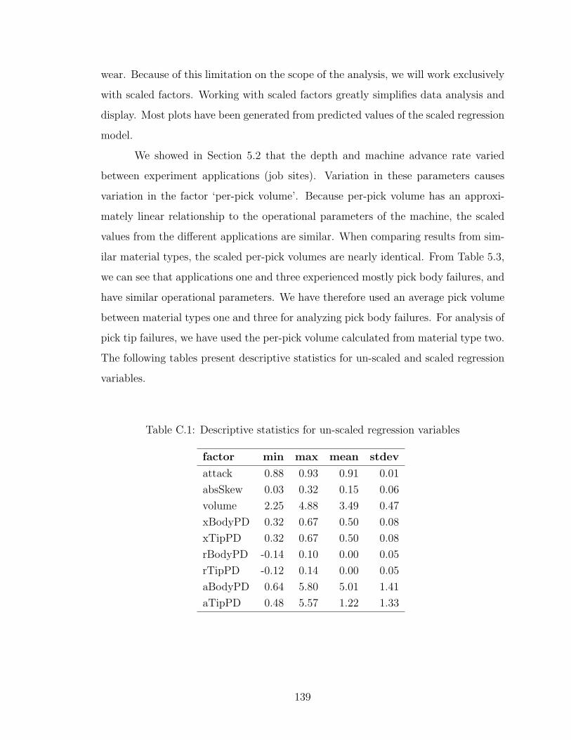
wear. Because of this limitation on the scope of the analysis, we will work exclusively
with scaled factors. Working with scaled factors greatly simplifies data analysis and
display. Most plots have been generated from predicted values of the scaled regression
model.
We showed in Section 5.2 that the depth and machine advance rate varied
between experiment applications (job sites). Variation in these parameters causes
variation in the factor ‘per-pick volume’. Because per-pick volume has an approxi-
mately linear relationship to the operational parameters of the machine, the scaled
values from the different applications are similar. When comparing results from sim-
ilar material types, the scaled per-pick volumes are nearly identical. From Table 5.3,
we can see that applications one and three experienced mostly pick body failures, and
have similar operational parameters. We have therefore used an average pick volume
between material types one and three for analyzing pick body failures. For analysis of
pick tip failures, we have used the per-pick volume calculated from material type two.
The following tables present descriptive statistics for un-scaled and scaled regression
variables.
Table C.1: Descriptive statistics for un-scaled regression variables
factor min max mean stdev
attack 0.88 0.93 0.91 0.01
absSkew 0.03 0.32 0.15 0.06
volume 2.25 4.88 3.49 0.47
xBodyPD 0.32 0.67 0.50 0.08
xTipPD 0.32 0.67 0.50 0.08
rBodyPD -0.14 0.10 0.00 0.05
rTipPD -0.12 0.14 0.00 0.05
aBodyPD 0.64 5.80 5.01 1.41
aTipPD 0.48 5.57 1.22 1.33
139
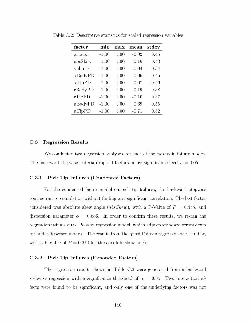
Table C.2: Descriptive statistics for scaled regression variables
factor min max mean stdev
attack -1.00 1.00 -0.02 0.45
absSkew -1.00 1.00 -0.16 0.43
volume -1.00 1.00 -0.04 0.34
xBodyPD -1.00 1.00 0.06 0.45
xTipPD -1.00 1.00 0.07 0.46
rBodyPD -1.00 1.00 0.19 0.38
rTipPD -1.00 1.00 -0.10 0.37
aBodyPD -1.00 1.00 0.69 0.55
aTipPD -1.00 1.00 -0.71 0.52
C.3 Regression Results
We conducted two regression analyses, for each of the two main failure modes.
The backward stepwise criteria dropped factors below significance level α = 0.05.
C.3.1 Pick Tip Failures (Condensed Factors)
For the condensed factor model on pick tip failures, the backward stepwise
routine ran to completion without finding any significant correlation. The last factor
considered was absolute skew angle (absSkew), with a P-Value of P = 0.455, and
dispersion parameter φ = 0.686. In order to confirm these results, we re-ran the
regression using a quasi Poisson regression model, which adjusts standard errors down
for underdispersed models. The results from the quasi Poisson regression were similar,
with a P-Value of P = 0.370 for the absolute skew angle.
C.3.2 Pick Tip Failures (Expanded Factors)
The regression results shown in Table C.3 were generated from a backward
stepwise regression with a significance threshold of α = 0.05. Two interaction ef-
fects were found to be significant, and only one of the underlying factors was not
140

individually significant. Figure C.1 shows the change in predicted failure probability
distribution for each main effect. Figure C.2 shows the change in predicted mean
failure rate for each interaction effect.
Table C.3: Regression results for tip failures for expanded factor model
Factor Name Coeff P-Value(Intercept) -0.463 0.0654rTipPD -0.124 0.8651aBodyPD 0.989 0.1060aTipPD 1.136 0.0226rTipPD x aBodyPD -2.985 0.0230rTipPD x aTipPD -3.639 0.05101 φ = 0.641
rTipPD Effects
0
0.2
0.4
0.6
0.8
1
0 1 2 3 4 5
Tip Failure Count
Pro
bab
ilit
y
Low rTipPD
High rTipPD
aBodyPD Effects
0
0.2
0.4
0.6
0.8
1
0 1 2 3 4 5
Tip Failure Count
Pro
bab
ilit
y
Low aBodyPD
High aBodyPD
aTipPD Effects
0
0.2
0.4
0.6
0.8
1
0 1 2 3 4 5 6 7 8 9 10 11 12 13 14 15
Tip Failure Count
Pro
bab
ilit
y
Low aTipPD
High aTipPD
Figure C.1: Plot of main effects on pick tip failure for expanded factor model
141

Figure C.2: Plot of interaction effects on pick tip failure for expanded-factor model
C.3.3 Pick Body Failures (Condensed Factors)
Regression on pick body failures, using condensed factors, returned two sig-
nificant predictors, and one significant interaction. Table C.4 lists coefficients and
significance. The dispersion parameter for this model is phi = 0.898.
Figure C.3 shows the change in predicted failure probability distribution for
each main effect. Figure C.4 shows the change in predicted mean failure rate for
the interaction effect. Note that this regression model was formed on the shortened
dataset (minus an outlier) described in a later section.
Table C.4: Regression results for body failures for expanded factor model
Factor Name Coeff P-Value(Intercept) -1.148 0.0000attack 0.816 0.1052absSkew 1.007 0.0422volume 1.748 0.0017attack x volume -2.441 0.01291 φ = 0.898
142

attack Effects
0
0.1
0.2
0.3
0.4
0.5
0.6
0.7
0.8
0.9
0 1 2 3 4 5
Body Failure Count
Pro
bab
ilit
yLow attack
High attack
absSkew Effects
0
0.2
0.4
0.6
0.8
1
0 1 2 3 4 5
Body Failure Count
Pro
bab
ilit
y
Low absSkew
High absSkew
volume Effects
0
0.2
0.4
0.6
0.8
1
1.2
0 1 2 3 4 5
Body Failure Count
Pro
bab
ilit
y
Low volume
high volume
Figure C.3: Plot of main effects on pick body failure for condensed factor model
Figure C.4: Plot of interaction effects on pick body failure, condensed factor model
143
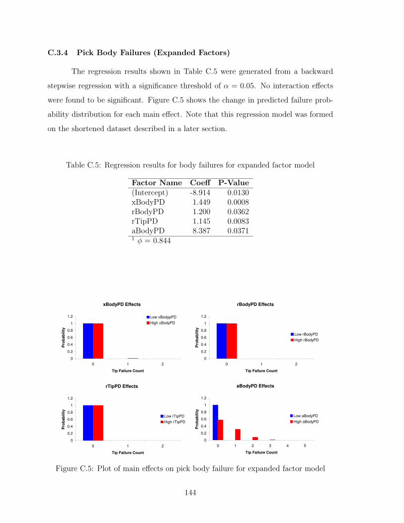
C.3.4 Pick Body Failures (Expanded Factors)
The regression results shown in Table C.5 were generated from a backward
stepwise regression with a significance threshold of α = 0.05. No interaction effects
were found to be significant. Figure C.5 shows the change in predicted failure prob-
ability distribution for each main effect. Note that this regression model was formed
on the shortened dataset described in a later section.
Table C.5: Regression results for body failures for expanded factor model
Factor Name Coeff P-Value(Intercept) -8.914 0.0130xBodyPD 1.449 0.0008rBodyPD 1.200 0.0362rTipPD 1.145 0.0083aBodyPD 8.387 0.03711 φ = 0.844
xBodyPD Effects
0
0.2
0.4
0.6
0.8
1
1.2
0 1 2
Tip Failure Count
Pro
bab
ilit
y
Low xBodypPD
High xBodyPD
rBodyPD Effects
0
0.2
0.4
0.6
0.8
1
1.2
0 1 2
Tip Failure Count
Pro
bab
ilit
y
Low rBodyPD
High rBodyPD
rTipPD Effects
0
0.2
0.4
0.6
0.8
1
1.2
0 1 2
Tip Failure Count
Pro
bab
ilit
y
Low rTipPD
High rTipPD
aBodyPD Effects
0
0.2
0.4
0.6
0.8
1
1.2
0 1 2 3 4 5
Tip Failure Count
Pro
bab
ilit
y
Low aBodyPD
High aBodyPD
Figure C.5: Plot of main effects on pick body failure for expanded factor model
144

C.4 Model Assumptions, Closeness, and Goodness of Fit
In an observational study, the factors being studied have only ordinary vari-
ation whereas, in a designed experiment, special variation would be intentionally
introduced to the model. For each factor, variation about the mean is smaller than
would be introduced in a designed experiment. For linear regressions, the R2 value
describes the proportion of the variance in bit wear attributable to the variance in
the factors of interest. When the factors of interest have smaller variance, they will
be smaller in proportion to any environmental noise. This has the effect of lowering
the R2 values of the regression. We expect this trend to also apply to the Poisson
regression, although there is no R2 value defined for non-linear models.
For Poisson regression models, the goodness of fit is typically described in
terms of overdispersion or underdispersion. Ideally, conditional variance of the re-
gression model is equal to the conditional mean (conditional mean and variance are
parameters of the regression model, not of the raw sample data). However, this
assumption rarely holds for real data. When the conditional variance is less than
(greater than) the conditional mean, the model is underdispersed (overdispersed).
The dispersion parameter for Poisson models, φ, is defined by V = φµ. A common
method for calculating dispersion parameter is to perform a quasi Poisson regression,
which fits the dispersion parameter using a maximum-likelihood method, rather than
fixing it at unity.
Well formed linear regression models exhibit normally distributed residuals,
and can be checked using a normal probability plot. Poisson regression residuals
are not normally distributed. There are however several versions of residuals that
can be used to assess Poisson model adequacy. In the text, “Regression Analysis of
Count Data,” Zorn[8] observes: “For count data there is no one residual that has zero
mean, constant variance, and symmetric distribution. ”This leads to several different
residuals according to which of these properties is felt to be most desirable.” For the
purposes of this study, we have primarily used the Anscombe residual. The Anscombe
residual is expected to be closest to normality for many Poisson regression models,
and can therefore be examined in a normal probability plot.
145

All of the models we have evaluated in this experiment exhibit underdispersion.
Underdispersion causes regression standard errors to be overestimated, therefore, our
models are conservative. However, a synopsis covering common sources of under- or
overdispersion in data provides certain insights into the phenomenon of bit failure.
A number of conditions can cause dispersion shifts in otherwise Poisson data, includ-
ing unobserved heterogeneity, zero-inflated/zero-truncated processes, and contagion
across events.
Overdispersion is often the result of “unobserved heterogeneity.” This cir-
cumstance occurs when observations with identical predictor values have different
observed values. Unobserved heterogeneity will be found where a relevant predictor
variable is missing from the model.
Poisson models with low mean predict a certain number of zero-value obser-
vations however, in many cases, the nature of the data generating process results in
greater or fewer zeros than expected. Zero inflated observations generally result from
special circumstances called dual regime data generating processes. Count data, with
zero-truncation, will result in underdispersed models. Overdispersion is correlated
with zero inflated data.
When positive contagion is present, high values of a particular observation
lead to correspondingly high values in other observations. Negative contagion is the
opposite: high values of one observation affects low values in other observations. As
explained by Zorn[8], “positive contagion leads to count data which are overdispersed;
negative contagion corresponds to underdispersed counts.”
Of the possible sources of underdispersion, negative contagion seems most
relevant. Assuming that contagion were present, we would expect high bit failures
in a particular position to result in lower bit failures in surrounding positions. Such
a phenomenon could be explained by differences in size between new and worn bits.
Bits with higher exposure to wear and breakage will be replaced more often than
their neighbors. When these bits are restored to new, they are taller than, and will
give a certain measure of protection to their already worn neighbors. This assessment
assumes that bits are changed immediately upon failure. If failed bits are not changed
146
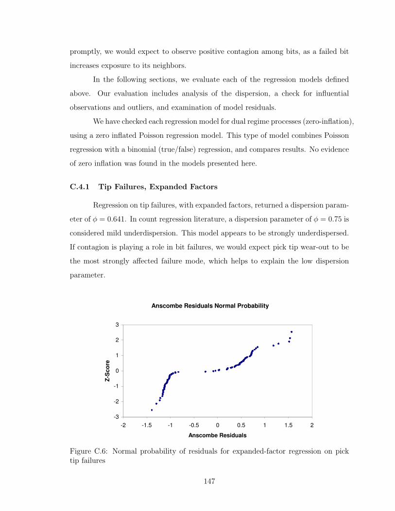
promptly, we would expect to observe positive contagion among bits, as a failed bit
increases exposure to its neighbors.
In the following sections, we evaluate each of the regression models defined
above. Our evaluation includes analysis of the dispersion, a check for influential
observations and outliers, and examination of model residuals.
We have checked each regression model for dual regime processes (zero-inflation),
using a zero inflated Poisson regression model. This type of model combines Poisson
regression with a binomial (true/false) regression, and compares results. No evidence
of zero inflation was found in the models presented here.
C.4.1 Tip Failures, Expanded Factors
Regression on tip failures, with expanded factors, returned a dispersion param-
eter of φ = 0.641. In count regression literature, a dispersion parameter of φ = 0.75 is
considered mild underdispersion. This model appears to be strongly underdispersed.
If contagion is playing a role in bit failures, we would expect pick tip wear-out to be
the most strongly affected failure mode, which helps to explain the low dispersion
parameter.
Anscombe Residuals Normal Probability
-3
-2
-1
0
1
2
3
-2 -1.5 -1 -0.5 0 0.5 1 1.5 2
Anscombe Residuals
Z-S
co
re
Figure C.6: Normal probability of residuals for expanded-factor regression on picktip failures
147

Another problem with this regression model becomes apparent upon examining
the residuals (Figure C.6). The residuals are obviously not normally distributed, and
in fact, indicate the presence of a bimodal distribution. In a previous section, we
described the pick tip failure mode as a simple wear-out phenomenon. Rather, there
seem to be two different failure modes in this data set. From our observation of
milling machine operation, especially in “alligatored” material, the second failure
mode is most likely sudden tip breakage, resulting from encounters with large rocks.
The problem we are observing here is not unobserved heterogeneity, and can-
not be fixed by adding additional predictor variables. This bimodal distribution is
a variant on the dual regime data generating process, and would ordinarily cause
overdispersion. However, the low dispersion value suggests that the bimodal nature
of the data is weak compared to the size of the response.
Influential observations are displayed in Figure C.7. This plot is based on
Cook’s distance, and can be helpful in identifying potential outliers. To statistically
analyze these influential observations, we performed a Bonferroni Outlier Test. We
found that observation number 47 (bit number 98) was the most extreme, but failed
to meet outlier criteria (i.e. PBonferroni < 0.1).
Influential Observations (Cook's Distance)
0
0.02
0.04
0.06
0.08
0.1
0.12
0.14
0.16
0.18
0 20 40 60 80 100 120
Bit Number
Co
ok S
tati
sti
c
Figure C.7: Influential observations among pick tip failures
148

C.4.2 Body Failures, Expanded Factors
An initial regression run on pick body failures, with both condensed and ex-
panded factors, showed a probable outlier at bit number 32 (observation number 10).
We have therefore dropped this observation from the dataset for all pick body regres-
sion models. Based on Cook’s distance, the adjusted dataset appears to produce a
more reasonably formed model (compare Figures C.9 and C.10). Additionally, the
resulting coefficients appear to be a better match with the theory. The comparison
of Table C.6 indicates that for the shortened dataset, body failures are more closely
correlated with body side geometry.
This regression model resulted in a dispersion parameter of φ = 0.844. While
the Anscombe residuals exhibit a slightly skewed distribution, the results generally
indicate a good fit to the Poisson distribution.
Deviance Residuals Normal Probability
-3
-2
-1
0
1
2
3
-2 -1.5 -1 -0.5 0 0.5 1 1.5 2 2.5
Deviance Residuals
Z-S
co
re
Figure C.8: Normal probability of residuals for expanded-factor regression on pickbody failures
149

Influential Observations (Cook's Distance)
0
0.2
0.4
0.6
0.8
1
1.2
1.4
1.6
1.8
0 20 40 60 80 100 120
Bit Number
Co
ok S
tati
sti
c
Figure C.9: Influential observations among pick body failures (expanded factors,including outlier)
Influential Observations (Cook's Distance)
0
0.02
0.04
0.06
0.08
0.1
0.12
0.14
0.16
0.18
0.2
0 20 40 60 80 100 120
Bit Number
Co
ok S
tati
sti
c
Figure C.10: Influential observations among pick body failures (expanded factors)
150

Table C.6: Comparison of coefficients for pick body outlier regression model
Outlier Model Short ModelFactor Name Coeff Factor Name Coeff(Intercept) -16.365 (Intercept) -8.914xBodyPD 1.609 xBodyPD 1.449xTipPD 15.964 rBodyPD 1.200rTipPD -8.588 rTipPD 1.145aBodyPD 17.176 aBodyPD 8.387aTipPD -0.066xTipPD x aBodyPD -17.848rTipPD x aTipPD -11.985
C.4.3 Body Failures, Condensed Factors
A backward stepwise regression on body failures, using condensed factors,
produced a model with dispersion parameter φ = 0.898. This value, being close
to unity, indicates a good fit with the Poisson distribution. Figure C.11 shows a
normal probability plot for the Anscombe residual. Although the Anscombe residual
is not always useful for non-linear regression, the “S” shape of the plot indicates lower
variance in the residuals than expected for a normal distribution.
Figure C.12 presents a plot of Cook’s distance for influential observations.
Comparison with Figure C.10 indicates that the two models on pick body failure are
quite similar. Note that both models use the shortened dataset, as described in the
preceding section.
151
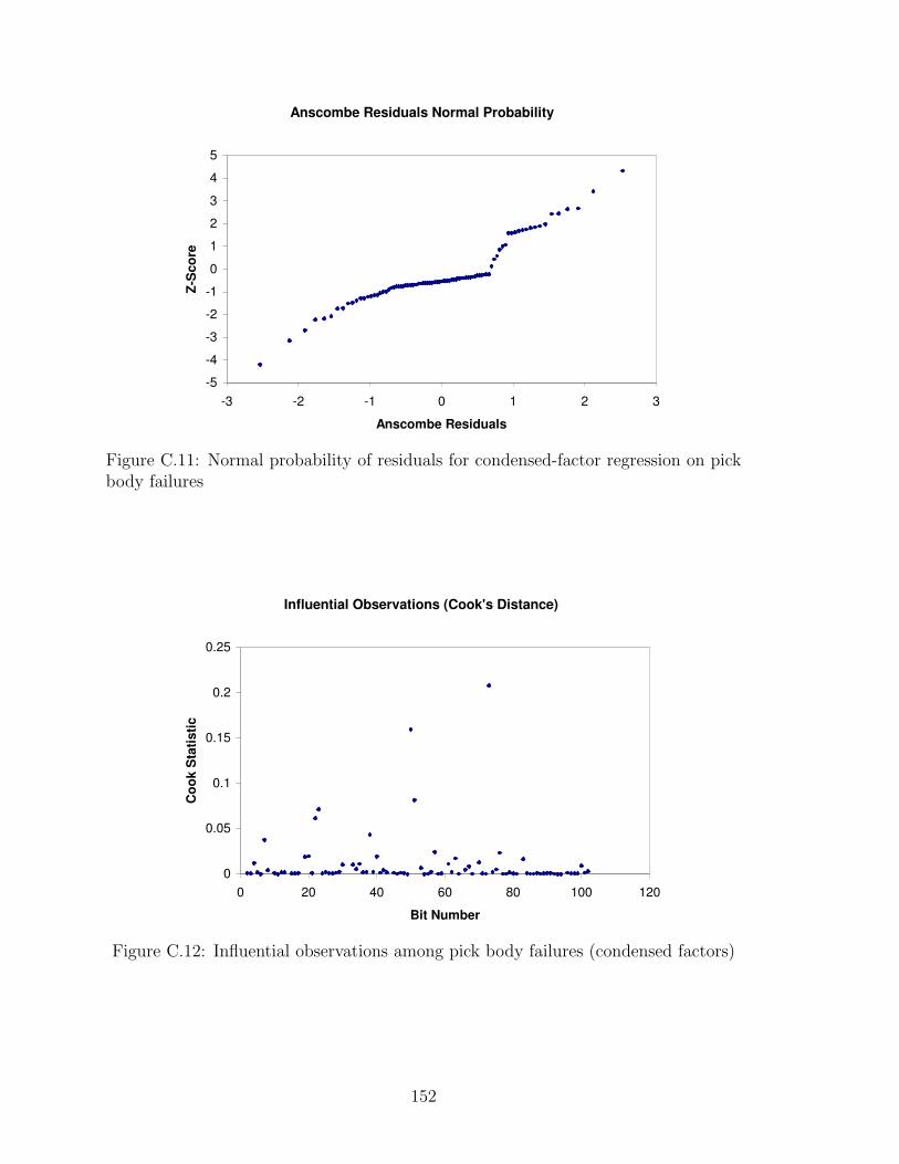
Anscombe Residuals Normal Probability
-5
-4
-3
-2
-1
0
1
2
3
4
5
-3 -2 -1 0 1 2 3
Anscombe Residuals
Z-S
co
re
Figure C.11: Normal probability of residuals for condensed-factor regression on pickbody failures
Influential Observations (Cook's Distance)
0
0.05
0.1
0.15
0.2
0.25
0 20 40 60 80 100 120
Bit Number
Co
ok S
tati
sti
c
Figure C.12: Influential observations among pick body failures (condensed factors)
152

C.5 Example Backward-Stepwise Regression
The following set of tables contain the steps taken in a backward stepwise
regression. This model regresses condensed factors against pick body failures, with a
significance threshold of α = 0.05. A total of 2 steps were required to arrive at the
final model. Note that the AIC value aids in Poisson model selection, much like R2
aids in linear model selection.
Step Number 0Factor Name Coeff P-Value(Intercept) -1.099 0.0000attack 0.893 0.0754absSkew 1.361 0.0231volume 1.801 0.0012attack x absSkew -1.001 0.3217attack x volume -2.506 0.0453absSkew x volume -0.710 0.61821 AIC = 123.61 φ = 0.871
Step Number 1Factor Name Coeff P-Value(Intercept) -1.092 0.0000attack 0.901 0.0713absSkew 1.277 0.0259volume 1.794 0.0013attack x absSkew -0.794 0.3794attack x volume -2.785 0.01291 AIC = 121.91 φ = 0.850
153

Step Number 2Factor Name Coeff P-Value(Intercept) -1.148 0.0000attack 0.816 0.1052absSkew 1.007 0.0422volume 1.748 0.0017attack x volume -2.441 0.01291 AIC = 120.71 φ = 0.842
154
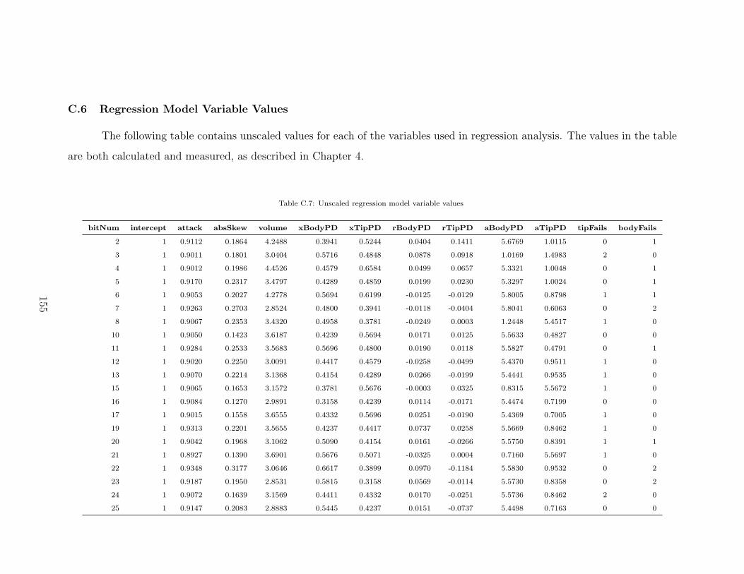
C.6 Regression Model Variable Values
The following table contains unscaled values for each of the variables used in regression analysis. The values in the table
are both calculated and measured, as described in Chapter 4.
Table C.7: Unscaled regression model variable values
bitNum intercept attack absSkew volume xBodyPD xTipPD rBodyPD rTipPD aBodyPD aTipPD tipFails bodyFails
2 1 0.9112 0.1864 4.2488 0.3941 0.5244 0.0404 0.1411 5.6769 1.0115 0 1
3 1 0.9011 0.1801 3.0404 0.5716 0.4848 0.0878 0.0918 1.0169 1.4983 2 0
4 1 0.9012 0.1986 4.4526 0.4579 0.6584 0.0499 0.0657 5.3321 1.0048 0 1
5 1 0.9170 0.2317 3.4797 0.4289 0.4859 0.0199 0.0230 5.3297 1.0024 0 1
6 1 0.9053 0.2027 4.2778 0.5694 0.6199 -0.0125 -0.0129 5.8005 0.8798 1 1
7 1 0.9263 0.2703 2.8524 0.4800 0.3941 -0.0118 -0.0404 5.8041 0.6063 0 2
8 1 0.9067 0.2353 3.4320 0.4958 0.3781 -0.0249 0.0003 1.2448 5.4517 1 0
10 1 0.9050 0.1423 3.6187 0.4239 0.5694 0.0171 0.0125 5.5633 0.4827 0 0
11 1 0.9284 0.2533 3.5683 0.5696 0.4800 0.0190 0.0118 5.5827 0.4791 0 1
12 1 0.9020 0.2250 3.0091 0.4417 0.4579 -0.0258 -0.0499 5.4370 0.9511 1 0
13 1 0.9070 0.2214 3.1368 0.4154 0.4289 0.0266 -0.0199 5.4441 0.9535 1 0
15 1 0.9065 0.1653 3.1572 0.3781 0.5676 -0.0003 0.0325 0.8315 5.5672 1 0
16 1 0.9084 0.1270 2.9891 0.3158 0.4239 0.0114 -0.0171 5.4474 0.7199 0 0
17 1 0.9015 0.1558 3.6555 0.4332 0.5696 0.0251 -0.0190 5.4369 0.7005 1 0
19 1 0.9313 0.2201 3.5655 0.4237 0.4417 0.0737 0.0258 5.5669 0.8462 1 0
20 1 0.9042 0.1968 3.1062 0.5090 0.4154 0.0161 -0.0266 5.5750 0.8391 1 1
21 1 0.8927 0.1390 3.6901 0.5676 0.5071 -0.0325 0.0004 0.7160 5.5697 1 0
22 1 0.9348 0.3177 3.0646 0.6617 0.3899 0.0970 -0.1184 5.5830 0.9532 0 2
23 1 0.9187 0.1950 2.8531 0.5815 0.3158 0.0569 -0.0114 5.5730 0.8358 0 2
24 1 0.9072 0.1639 3.1569 0.4411 0.4332 0.0170 -0.0251 5.5736 0.8462 2 0
25 1 0.9147 0.2083 2.8883 0.5445 0.4237 0.0151 -0.0737 5.4498 0.7163 0 0
155

Table C.7: continued
bitNum intercept attack absSkew volume xBodyPD xTipPD rBodyPD rTipPD aBodyPD aTipPD tipFails bodyFails
26 1 0.8939 0.1699 3.4831 0.4949 0.5090 0.0079 -0.0161 5.4339 0.7081 0 0
27 1 0.8893 0.1390 3.5038 0.5071 0.5064 -0.0004 0.0073 0.7135 5.4373 1 0
28 1 0.8986 0.1580 3.6827 0.4738 0.6617 -0.0170 -0.0970 5.4343 0.7002 0 0
29 1 0.9054 0.1903 3.7880 0.5721 0.5815 0.0202 -0.0569 5.4341 0.7102 1 0
30 1 0.9053 0.1926 3.3064 0.5603 0.4411 0.0365 -0.0170 5.4345 0.7095 0 1
32 1 0.9080 0.2122 3.6785 0.4442 0.5445 0.0241 -0.0151 5.5630 0.8334 0 2
33 1 0.9263 0.2035 3.8634 0.6251 0.4949 0.0412 -0.0079 5.5676 0.8493 0 0
34 1 0.9204 0.2354 3.5652 0.5064 0.5230 -0.0073 -0.0012 0.8459 5.5539 0 0
35 1 0.8997 0.2120 3.5715 0.5173 0.4738 0.0406 0.0170 5.5648 0.8488 0 1
36 1 0.9175 0.1739 3.5746 0.3513 0.5721 -0.0059 -0.0202 5.5631 0.8491 1 0
37 1 0.9172 0.2023 3.5522 0.4965 0.5603 -0.0196 -0.0365 5.5701 0.8487 0 0
38 1 0.8936 0.1905 3.2070 0.6147 0.4442 -0.0298 -0.0241 5.4315 0.7202 1 1
39 1 0.8910 0.1701 3.6941 0.4714 0.6251 -0.0042 -0.0412 5.4384 0.7156 1 0
40 1 0.9318 0.1870 3.4880 0.5230 0.4923 0.0012 -0.0125 0.7293 5.4560 1 0
41 1 0.9111 0.1968 2.9774 0.4398 0.5173 -0.0877 -0.0406 5.4322 0.7184 0 0
42 1 0.9124 0.2542 2.8863 0.6653 0.3513 -0.0657 0.0059 5.4350 0.7201 0 0
43 1 0.8972 0.2516 2.9704 0.4848 0.4965 -0.0918 0.0196 4.7849 0.7131 1 0
45 1 0.9045 0.1521 3.7792 0.4840 0.6147 -0.0980 0.0298 5.5630 0.8516 0 0
46 1 0.8943 0.1517 2.9671 0.5244 0.4714 -0.1411 0.0042 5.2717 0.8448 0 0
47 1 0.8904 0.2068 3.3047 0.4923 0.5716 0.0125 -0.0878 0.8272 5.2663 1 0
48 1 0.9120 0.2647 3.7069 0.6584 0.4398 -0.0657 0.0877 5.2784 0.8510 0 1
49 1 0.9233 0.2482 4.2030 0.4859 0.6653 -0.0230 0.0657 5.2808 0.8481 1 1
50 1 0.9342 0.2305 4.8831 0.4836 0.4958 0.0036 0.0249 5.6396 5.0384 2 0
51 1 0.9133 0.2250 4.0767 0.6199 0.4840 0.0129 0.0980 5.4034 0.7202 1 3
53 1 0.8929 0.0829 4.4607 0.4259 0.5340 0.0703 0.1325 5.6854 1.0272 0 1
54 1 0.8915 0.0846 2.2511 0.4836 0.5004 -0.0036 0.0796 0.6435 1.0162 2 0
55 1 0.9047 0.1414 4.5331 0.5862 0.6168 0.0638 0.0313 5.3335 1.0337 1 1
156
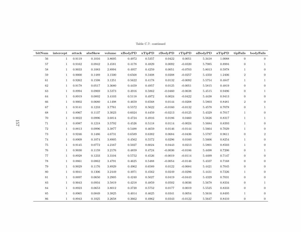
Table C.7: continued
bitNum intercept attack absSkew volume xBodyPD xTipPD rBodyPD rTipPD aBodyPD aTipPD tipFails bodyFails
56 1 0.9119 0.1016 3.8695 0.4972 0.5357 0.0422 0.0051 5.3418 1.0088 0 0
57 1 0.9162 0.0942 3.4581 0.4178 0.4829 0.0092 -0.0320 5.7985 0.8994 0 1
58 1 0.9033 0.1083 2.8994 0.4957 0.4259 0.0051 -0.0703 5.8013 0.5978 1 0
59 1 0.9000 0.1489 3.1500 0.6568 0.3408 0.0208 -0.0257 5.4350 1.2406 2 0
61 1 0.9262 0.1598 3.1251 0.5622 0.4178 0.0132 -0.0092 5.5754 0.4847 1 1
62 1 0.9178 0.0517 3.3680 0.4459 0.4957 0.0125 -0.0051 5.5815 0.4819 0 0
63 1 0.8994 0.0969 3.5373 0.4916 0.5862 -0.0460 -0.0638 5.4515 0.9496 0 1
64 1 0.8919 0.0892 3.4103 0.5118 0.4972 0.0024 -0.0422 5.4438 0.9413 0 0
66 1 0.9002 0.0680 4.1498 0.4659 0.6568 0.0144 -0.0208 5.5803 0.8481 2 0
67 1 0.9141 0.1233 3.7761 0.5572 0.5622 -0.0160 -0.0132 5.4578 0.7078 0 1
68 1 0.8967 0.1137 3.3023 0.6024 0.4459 -0.0213 -0.0125 5.4329 0.7017 1 0
70 1 0.9022 0.0996 3.6814 0.4724 0.4916 0.0186 0.0460 5.5626 0.8317 1 1
71 1 0.8987 0.1218 3.5792 0.4526 0.5118 0.0114 -0.0024 5.5684 0.8393 1 0
72 1 0.8813 0.0996 3.3877 0.5488 0.4659 0.0146 -0.0144 5.5664 0.7029 1 0
73 1 0.9246 0.1486 4.6731 0.6589 0.6382 0.0684 -0.0436 5.5787 0.9611 0 2
74 1 0.8909 0.1074 3.8905 0.4562 0.5572 0.0296 0.0160 5.5606 0.8254 1 0
75 1 0.9145 0.0772 4.2167 0.5027 0.6024 0.0443 0.0213 5.5801 0.8503 1 0
76 1 0.9030 0.1159 3.2176 0.4859 0.4724 -0.0036 -0.0186 5.4498 0.7206 0 1
77 1 0.8928 0.1233 3.3104 0.5752 0.4526 -0.0019 -0.0114 5.4499 0.7147 0 0
78 1 0.8861 0.0862 3.4791 0.4625 0.5488 -0.0054 -0.0146 5.4337 0.7168 0 0
79 1 0.9029 0.1176 3.8929 0.4962 0.6589 0.0122 -0.0684 5.4421 0.7045 0 0
80 1 0.9041 0.1306 3.2449 0.4971 0.4562 0.0249 -0.0296 5.4431 0.7226 1 0
81 1 0.8897 0.0650 3.2905 0.4240 0.5027 0.0419 -0.0443 5.4329 0.7031 0 0
83 1 0.9043 0.0934 3.5819 0.4218 0.4859 0.0502 0.0036 5.5678 0.8334 0 1
84 1 0.8923 0.0653 3.8012 0.3720 0.5752 0.0177 0.0019 5.5525 0.8333 0 0
85 1 0.8965 0.0849 3.3825 0.4014 0.4625 0.0341 0.0054 5.5616 0.8495 1 0
86 1 0.8943 0.1025 3.2658 0.3662 0.4962 0.0343 -0.0122 5.5647 0.8410 0 0
157

Table C.7: continued
bitNum intercept attack absSkew volume xBodyPD xTipPD rBodyPD rTipPD aBodyPD aTipPD tipFails bodyFails
87 1 0.9087 0.1245 3.6642 0.5897 0.4971 0.0290 -0.0249 5.5713 0.8401 1 0
88 1 0.8955 0.1435 2.9388 0.4948 0.4240 -0.0120 -0.0419 5.5660 0.8502 1 0
89 1 0.8931 0.2022 2.9639 0.6005 0.4218 -0.0310 -0.0502 5.4402 0.7154 1 0
90 1 0.9126 0.1562 2.9883 0.6284 0.3720 0.0099 -0.0177 5.4536 0.7307 0 0
91 1 0.9110 0.1602 2.9193 0.5860 0.4014 -0.0126 -0.0341 5.4461 0.7216 1 0
92 1 0.9061 0.1578 2.3621 0.4156 0.3662 -0.0663 -0.0343 5.4485 0.7184 0 0
93 1 0.8807 0.0556 3.1750 0.3827 0.5897 -0.0921 -0.0290 5.4170 0.7119 0 0
94 1 0.8768 0.1076 3.2082 0.5186 0.4948 -0.0873 0.0120 5.4344 0.7172 1 0
96 1 0.8968 0.0717 3.8501 0.5192 0.6005 -0.0831 0.0310 5.5542 0.8430 1 0
97 1 0.8897 0.0554 3.6090 0.5340 0.6284 -0.1325 -0.0099 5.2560 0.8295 0 0
98 1 0.8870 0.1085 3.5845 0.5004 0.5860 -0.0796 0.0126 5.2669 0.8371 2 0
99 1 0.8854 0.1261 3.4717 0.6168 0.4156 -0.0313 0.0663 5.2495 0.8347 1 0
100 1 0.9285 0.0412 3.3251 0.5357 0.3827 -0.0051 0.0921 5.2744 0.8662 2 0
101 1 0.9105 0.0335 3.6488 0.3408 0.5186 0.0257 0.0873 5.0426 0.8488 1 0
102 1 0.9133 0.0625 3.9062 0.4829 0.5192 0.0320 0.0831 5.3838 0.7290 1 0
158

Appendix D
Cutter Head Measurement
We used a Romer/Cimcore 10 foot Infinite Arm model CMM to measure the
location and orientation of each pick on a selected cutter head. These measurements
were taken on empty holders, and then transformed based on the shape of the pick
to be used in our study. This approach is possible because of the relatively low
dimensional variation between picks. Figure D.1 shows the setup and apparatus used
in collecting measurements.
In order to more accurately represent cutting conditions, we measured the
completely assembled cutter head (with its drive system). We used the drive system
mounting surfaces as measurement reference surfaces. Because the CMM arm could
not reach completely around the cutter head, we were required to reposition the CMM
three times while taking measurements. To accomplish the repositioning, we fastened
four large rigid plates to the cutter head skin at each quadrant. One of the plates
can be seen in Figure D.1.
159
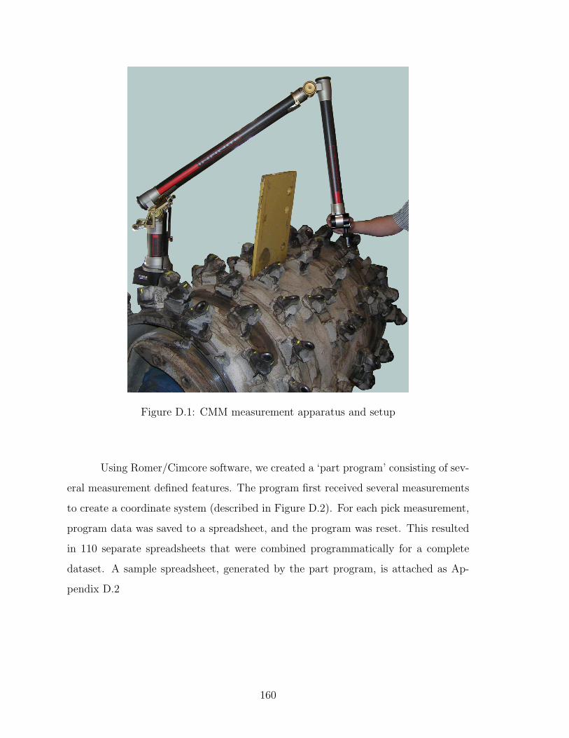
Figure D.1: CMM measurement apparatus and setup
Using Romer/Cimcore software, we created a ‘part program’ consisting of sev-
eral measurement defined features. The program first received several measurements
to create a coordinate system (described in Figure D.2). For each pick measurement,
program data was saved to a spreadsheet, and the program was reset. This resulted
in 110 separate spreadsheets that were combined programmatically for a complete
dataset. A sample spreadsheet, generated by the part program, is attached as Ap-
pendix D.2
160

Support Shaft End Face
Z-Axis
Support Shaft OD
Input Shaft OD
Pick Holder 52
X-Axis
Y-Axis
Figure D.2: Coordinate system created in the CMM part program
The data returned by the part program required post-processing to convert
from the CMM reference frame to measures more commonly used in pick lacing
specifications. Data returned by the part program consisted of clock angle, forward
angle, side angle, block radius, and axial distance. Using several simple trigonometric
operations, we transformed the foregoing variables into Drum Angle, Attack Angle,
Skew Angle, Tip Radius, and Axial Position. Each of these variables are further
defined here, and in Section 2.3.2. A listing of chapter variables, relative to the
geometry presented in Figure D.2, is provided in Section D.1.
Equation D.1 shows the transform for converting clock angle to the angular
position required for a lacing specification. The contributing variables are illustrated
in Figures D.3, D.4, and D.5. This equation depends primarily on the length and
orientation of the pick.
161

lp = la cos (sa)
caa = arctan
[lp sin (fa)
rb + lp cos (fa)
]
φd =
−(ca + caa) + ca1 if ca + caa < 3
−(ca + caa) + ca1 + 2π if ca + caa ≥ 3(D.1)
Where:
la = Actual bit length
lp = Projected bit length
sa = Block side angle
fa = Forward angle
rb = Radial distance to block reference point
ca = Clock angle
caa = Clock angle adjustment
ca1 = Adjusted clock angle for bit 1
φd = Drum angle
Equation D.2 shows the calculation for transforming block radius, rb, into
pick tip radius, R. The geometry for this calculation is quite simple. Contributing
variables are illustrated in Figure D.3.
162
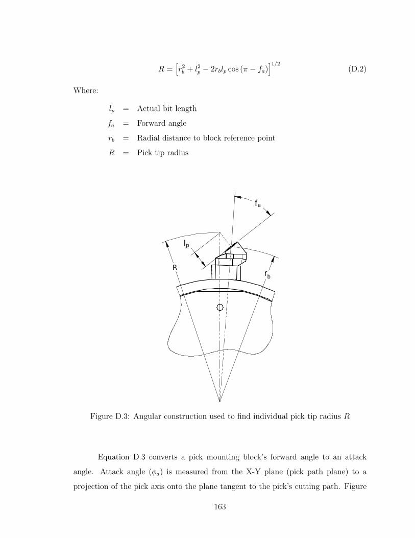
R =[r2b + l2p − 2rblp cos (π − fa)
]1/2(D.2)
Where:
lp = Actual bit length
fa = Forward angle
rb = Radial distance to block reference point
R = Pick tip radius
Figure D.3: Angular construction used to find individual pick tip radius R
Equation D.3 converts a pick mounting block’s forward angle to an attack
angle. Attack angle (φa) is measured from the X-Y plane (pick path plane) to a
projection of the pick axis onto the plane tangent to the pick’s cutting path. Figure
163
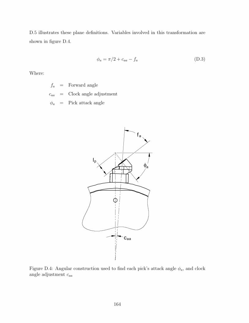
D.5 illustrates these plane definitions. Variables involved in this transformation are
shown in figure D.4.
φa = π/2 + caa − fa (D.3)
Where:
fa = Forward angle
caa = Clock angle adjustment
φa = Pick attack angle
Figure D.4: Angular construction used to find each pick’s attack angle φa, and clockangle adjustment caa
164

φs = arctan
[sin (sa)
cos (φa) cos (sa)
](D.4)
Where:
sa = Block side angle
φa = Pick attack angle
φs = Pick skew angle
Block Reference Point
φ
pl
a
s a
AxisBlock Bore
s
l
Block BoreAxis Projection
Figure D.5: Illustration of variables for transforming measured side angle (sa) intoskew angle φs
Some of the features used to calculate each pick’s Skew Angle are shown in
Figure D.5. As described in Equation D.4, skew angle can be determined solely from
a block’s side angle and attack angle. Side angle was directly measured with the
CMM, and attack angle was calculated in Equation D.3.
165

The CMM setup measured mounting block axial position based on the end
surface of the cutter head support shaft. In theory, standard lacing specifications
measure the pick tip axial position from the edge of the cutter head skin (as shown
in engineering drawings). However, in practice, axial position is more appropriately
measured from the zero-bit. The zero-bit is the first pick where the tip is axially
aligned with the left side of the cutter head skin (viewed from the front of the ma-
chine). Equation D.5 converts axial position as measured by the CMM to that of the
lacing specification.
Pick skew angle (φs) is defined in terms of a plane tangent to the path of the
pick tip. This allows us to find axial offset from skew angle and pick length, without
transformation. The pick skew angle was calculated using Equation D.4.
Da = ad0 − [ad − la sin (φs)] (D.5)
Where:
ad0 = Axial distance from CMM origin to zero-bit
ad = Axial distance from CMM origin to block reference point
la = Actual bit length
φs = Pick skew angle
Da = Axial coordinate of pick tip
166

D.1 Variables Summary
Block measurements, based on CMM coordinate system:
ca = Clock angle, measured from X-Z plane (based on bit number 52) to
origin of individual block, around cutter head axis of rotation
caa = Clock angle adjustment, converting from block clock angle to pick tip
clock angle
ca1 = Adjusted clock angle, measured from origin X-Z plane to reference point
of block number 1
fa = Forward angle, measured from radius vector for the block reference
point to the axis of the block’s bore, projected onto the X-Y plane
sa = Block side angle, the smallest angle from the block bore axis to the pick
path plane
rb = Radial distance to block origin, measured from CMM coordinate system
z-axis
ad = Axial distance from cutter head CMM coordinate system origin to block
reference point
ad0 = Axial distance from CMM coordinate system origin to tip of lacing
pattern zero-bit (bit number 9)
Bit parameters, measured in lacing specification coordinate system:
φd = Drum angle (or angular position), measured from cutter head skin
origin-line to individual pick tip
φa = Pick attack angle, measured from pick path plane to pick axis, projected
onto cut tangent plane
φs = Pick skew angle, measured from the X-Y plane to the projection of the
pick axis onto the cut-tangent plane
R = Individual pick tip radius, from rotational axis of cutter head
Da = Axial coordinate of a pick tip location, relative to reference point on
edge of cutter head skin
Pick related parameters:
la = Actual bit length (new), measured from shoulder to tip
lp = Projected bit length (new), actual bit length projected onto pick path
plane (X-Y plane in CMM coordinate system)
167

D.2 Sample Part-Program Report
����� ����� ����� � ���� � � ��� � �����
� ����� ����� ����� ����� 0.000������ � ����� ����� ����� ����� 0.000
� ����� ����� ����� ����� 0.000������� ������ ����� ����� ����� 3.137 3.037
����� ����� ����� � ���� � � ��� � �����
� ����� ����� ����� ����� 0.000������ � ����� ����� ����� ����� 0.000
� ����� ����� ����� ������ 57.379������� ������ ����� ����� ���� 1.701 1.601
���� ���� ������������ ������ ����� ����� ������ 57.379 57.279
����� ����� ����� � ���� � � ��� � �����
� ����� ����� ����� ����� 0.000����� � ����� ����� ����� ����� 0.000
� ����� ����� ����� ����� 0.000
����� ����� ����� � ���� � � ��� � �����
� ����� ����� ����� ��!�!"� -16.647������ � ����� ����� ����� ����� 0.000
� ����� ����� ����� ��! � 1.625������� ������ ����� ����� ����! -0.014
����� ����� ����� � ���� � � ��� � �����
� ����� ����� ����� ��!�!"� -16.647����� � ����� ����� ����� ����� 0.000
� ����� ����� ����� ����� 0.000
�������� ������ ����� ����� �!�!"� 16.647 16.547
INSPECTION REPORT 7/1/2005 13:58
� ��� ������
� ��� ������
������
����� ��� ������
����� ��� ���� �����
����� ��� ���� ����
�������� �����
����� ����� ����� � ���� � � ��� � �����
������
� ����� ����� ����� "!���� 46.791
�������� ������ ����� ����� �!�!�� 16.615 16.515
����� ����� ����� ����� ������� -91.187
����� ����� ����� ����� ����� � -17.528
����� ����� ����� ����� ��� " 39.224
���� �����
������� �����
���
����� ��������
���� !�����
���� �����
168
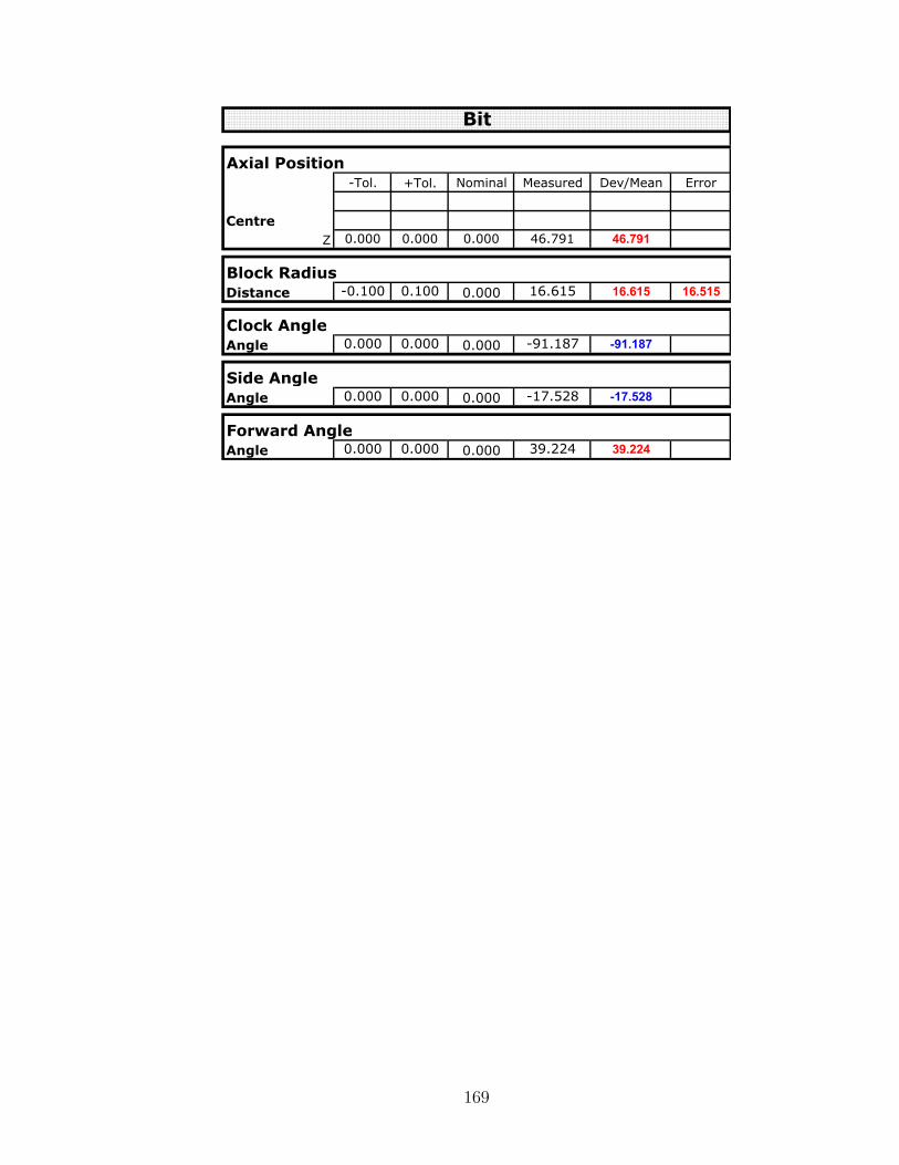
����� ����� ����� � ���� � � ��� � �����
������
� ����� ����� ����� ������ ������
������ ������ ����� ����� ������ ������ ������
��� � ����� ����� ����� ������� ������
��� � ����� ����� ����� ������� �����
��� � ����� ����� ����� ����� ����
� ������ �
��� ���������
� ��������
�������� �
���������� �
���
169

170
Bibliography
[1] S. Rogers and B. Roberts, “Wear mechanisms associated with rock excavation
using attack picks,” Mining Science and Technology, vol. 12, pp. 317–323, 1991.
[2] K. W. Chase and D. L. Mahlum, “StratapaxTMcomputer program,” tech. rep.,
Special Products Division, Sandia Laboratories, 1978.
[3] M. H. D. Hartog, R. Babuska, H. J. R. Deketh, M. A. Grima, P. N. W. Verhoef,
and H. B. Verbruggen, “Forecasting of rock trencher performance using a fuzzy
logic approach,” International journal of Approximate Reasoning, vol. 16, pp. 43–
56, 1997.
[4] C. F. Wingquist, B. D. Hanson, W. W. Roepke, and T. A. Myren, “Conical bit
rotation as a function of selected cutting parameters,” Tech. Rep. 8983, United
States Bureau of Mines, 1985.
[5] B. Tiryaki, “Computer-aided design of precision control linkages in the class-
room,” tech. rep., Dynamic Systems & Control Division of The American Society
of Mechanical Engineers, July 2004. Published separately under reference number
“80-WA/DSC-39”.
[6] MathPages, “Net area and green’s theorem.” http://www.mathpages.com/home/
kmath201.htm, July 2005.
[7] J. Gao, K. W. Chase, and S. P. Magleby, “Comparison of assembly tolerance
analysis by the direct linearization and modified monte carlo simulation methods,”
in Proceedings of the ASME Design Engineering Technical Conferences, vol. 1,
(Boston, MA), pp. 353–360, September 1995.
171

[8] A. C. Cameron and P. K. Trivedi, Regression Analysis of Count Data. No. 30 in
Econometric Society Monographs, Cambridge University Press, 1998.
172
Related Documents