Default Probabilities of Privately Held Firms Jin-Chuan Duan * , Baeho Kim † ,, Woojin Kim ‡ and Donghwa Shin § (This version: July 12, 2017) ¶ ABSTRACT We estimate term structures of default probabilities for private firms using data consisting of 1,759 default events from 29,894 firms between 1999 and 2014. Each firm’s default likelihood is characterized by a forward intensity model employing macro risk factors and firm-specific attributes. As private firms do not have traded stock prices, we devise a methodology to obtain a public-firm equivalent distance- to-default by projection which references the distance-to-defaults of public firms with comparable attributes. The fitted model provides accurate multi-period fore- casts of defaults, leading to both economically and statistically significant benefits over benchmark models. The reported interest rates charged to private firms are reflective of the estimated default term structure. Keywords: Default probability; Term structure; Privately held firm; Interest charge JEL Classification: E43, E47, G33 * Risk Management Institute and Department of Finance, National University of Singapore. E-mail: [email protected]. † Corresponding Author. Korea University Business School, Anam-dong, Sungbuk-gu, Seoul 136-701, South Korea, Phone +82 2 3290 2626, Fax +82 2 922 7220, E-mail: [email protected]. ‡ Seoul National University Business School. E-mail: [email protected]. § Department of Economics, Princeton University. E-mail: [email protected]. ¶ We are grateful for helpful discussions and insightful comments to Wan-Chien Chiu, John Finnerty, Marco Geidosch, Suk-Joong Kim, Yongjae Kwon, Dragon Yongjun Tang and participants of the 6th Annual Risk Management Conference, the 8th Conference of Asia-Pacific Association of Derivatives, the 2nd Conference on Credit Analysis and Risk Management, 2013 Annual Meeting of the Financial Man- agement Association International, the 8th International Conference on Asia-Pacific Financial Markets, and 2015 FMA Asian Meeting. We thank the Risk Management Institute (RMI) at the National Uni- versity of Singapore for the support provided to this research, and Qianqian Wan, Hanbaek Lee and Yeong Joon Cho for excellent data assistance. Baeho Kim is grateful for support from the SK-SUPEX Fellowship of Korea University Business School, and Woojin Kim appreciates support from the Institute of Management Research at Seoul National University.

Welcome message from author
This document is posted to help you gain knowledge. Please leave a comment to let me know what you think about it! Share it to your friends and learn new things together.
Transcript
Default Probabilities of Privately Held Firms
Jin-Chuan Duan∗, Baeho Kim†,, Woojin Kim‡ and Donghwa Shin§
(This version: July 12, 2017)¶
ABSTRACT
We estimate term structures of default probabilities for private firms using data
consisting of 1,759 default events from 29,894 firms between 1999 and 2014. Each
firm’s default likelihood is characterized by a forward intensity model employing
macro risk factors and firm-specific attributes. As private firms do not have traded
stock prices, we devise a methodology to obtain a public-firm equivalent distance-
to-default by projection which references the distance-to-defaults of public firms
with comparable attributes. The fitted model provides accurate multi-period fore-
casts of defaults, leading to both economically and statistically significant benefits
over benchmark models. The reported interest rates charged to private firms are
reflective of the estimated default term structure.
Keywords: Default probability; Term structure; Privately held firm; Interest charge
JEL Classification: E43, E47, G33
∗Risk Management Institute and Department of Finance, National University of Singapore. E-mail:[email protected].†Corresponding Author. Korea University Business School, Anam-dong, Sungbuk-gu, Seoul 136-701,
South Korea, Phone +82 2 3290 2626, Fax +82 2 922 7220, E-mail: [email protected].‡Seoul National University Business School. E-mail: [email protected].§Department of Economics, Princeton University. E-mail: [email protected].¶We are grateful for helpful discussions and insightful comments to Wan-Chien Chiu, John Finnerty,
Marco Geidosch, Suk-Joong Kim, Yongjae Kwon, Dragon Yongjun Tang and participants of the 6thAnnual Risk Management Conference, the 8th Conference of Asia-Pacific Association of Derivatives, the2nd Conference on Credit Analysis and Risk Management, 2013 Annual Meeting of the Financial Man-agement Association International, the 8th International Conference on Asia-Pacific Financial Markets,and 2015 FMA Asian Meeting. We thank the Risk Management Institute (RMI) at the National Uni-versity of Singapore for the support provided to this research, and Qianqian Wan, Hanbaek Lee andYeong Joon Cho for excellent data assistance. Baeho Kim is grateful for support from the SK-SUPEXFellowship of Korea University Business School, and Woojin Kim appreciates support from the Instituteof Management Research at Seoul National University.

1. Introduction
The appropriate assessment of credit risk is not only of interest to academics, but even
more important for commercial lenders who must decide both whether to lend and how
much of a credit spread to charge for a given loan application. Although the academic
literature has been rife with studies of credit risk assessment ever since the early works of
Altman (1968), most of the related works, whether structural or non-structural in nature,
focus on publicly-traded firms (see Beaver (1966), Bharath & Shumway (2008), Campbell,
Hilscher & Szilagyi (2008), Chava & Jarrow (2004), Hillegeist, Keating & Cram (2004),
Ohlson (1980), Duffie, Saita & Wang (2007), Duan, Sun & Wang (2012), and many
others).
In contrast, defaults of privately held firms mainly remain in the realm of commercial
interest, and the research findings are kept proprietary. Academic research on the subject
of private firm defaults is skimpy. Other than Altman (2013)’s work, there are only
a few studies, mostly from the practitioners’ perspective, that examine credit risk of
private firms. For instance, Cangemi, Servigny & Friedman (2003) of Standard and
Poor’s examined the default risk of French private firms based on maximum expected
utility (MEU) approach. Falkenstein, Boral & Carty (2000) of Moody’s proposed a non-
structural approach to assess credit risk of private firms in the U.S. market. This relative
paucity of academic attention is partly due to the lack of publicly available data on
privately held firms. Even if financial statement data on privately held firms were widely
available, there is no market data, such as stock prices, to offer an important dimension of
timely information on these firms. As recent advancements in credit risk model typically
requires some form of market information, the absence of market data thus poses an
additional obstacle to studying defaults of private firms.
In this study, we devise a way to utilize timely market information. Specifically, we
estimate a powerful market information measure, known as distance-to-default (DTD),
for private firms by referring to the universe of public firms for similar characteristics. Our
approach can thus help assess whether using a modified version of the credit risk model
that requires market data to predict defaults of private firms actually adds any value.
In addition, we adopt the newly developed doubly stochastic Poisson forward-intensity
default modelling technique of Duan et al. (2012) to estimate the term structure of default
probabilities for privately held firms. By directly modelling forward intensities, one can
directly relate future defaults in any particular time period to the current information
set characterized by some market-wide common risk factors and firm-specific attributes.
1

Using forward as opposed to spot intensities, one in effect bypasses the challenging task
of modelling very high dimensional time series of covariates arising from firm-specific
attributes due to the sheer number of firms in the data sample.
We investigate both financial and non-financial private firms. Needless to say, finan-
cial firms are of great importance. Despite their relevance, the literature on corporate
default/bankruptcy typically ignore financial firms, in part because financial firms are
highly leveraged making them somewhat distinct from non-financial firms. Technically
speaking, reliable DTDs for financial firms is more difficult to obtain. Duan et al. (2012),
however, demonstrated that using properly estimated DTDs in corporate default predic-
tions can yield a universal model (i.e., financial and non-financial firms share the same
default prediction model) that performs equally well for the subsamples of financial and
non-financial firms in terms of the accuracy ratio.1
In this paper, we evaluate the credit risk of Korean private firms, both financial and
non-financial, based on aforementioned approach. There are three broad reasons why
we focus on Korea. First, Korean regulations on default disclosures allow us to assem-
ble a comprehensive dataset on all default events by all corporations, both public and
private, and all individuals who have checking accounts.2 Whenever there is a bounced
check issued by any entity within the Korean banking system, Korea Financial Telecom-
munications and Clearing Institute (KFTC), the official check clearing house in Korea,
discloses the detailed identity of the check issuers, including the names, addresses, the
date of default, and the first 7 digits of identification codes. This unique feature of Korean
market allows us to assemble a dataset that is not only large but also comprehensive by
containing the population of all defaults triggered by bounced checks for all businesses
so that it can be free from potential selection bias. This is a significant advantage over
existing commercial databases in the U.S. in terms of the quality and range of default
information.
Second, firm-specific attributes for our sample of private firms are more reliable,
as all the firms are externally audited. Specifically, Korean auditing regulations require
all corporations whose total assets exceed KRW 10 billion (roughly USD 10 million) to
hire an external auditor to audit their financial statements. We are unaware of similar
regulations in other markets which require mandatory external auditing even for private
firms. For example, there is little known about financial information of large commodity
1For further details on estimating DTDs for financial firms, please refer to Duan & Wang (2012).2Unlike in U.S. where anyone with a valid address can open up a checking account and issue personal
checks, such payment mechanism is rarely used by common households in Korea. Rather, checkingaccounts are mostly used by businesses, both corporations and sole proprietorships.
2

trading companies, as most of them are private, except for Glencore, even though they
account for the majority of commodity trading around the world. In fact, one of Moody’s
reports on private firm defaults (Moody’s RiskCalc 3.1 Korea Report) documents that
accuracy ratio for audited firms in Korea is higher than the corresponding number for
U.S. private firms. The higher ratio may be attributed to higher quality of information
provided by the auditing process. This feature should clearly enhance the accuracy of the
default prediction model.
Finally, not only is financial information of Korean private firms externally audited,
but also it contains detailed information on the amount and interest rates charged for
short-term and long-term loans, as well as repayment schedule and collateral information
by each loan facility providing institution. We are also unaware of availability of such
detailed information for private firms in other markets, including U.S. The availability of
forward-looking information on interest charges conditional on maturity allows us to test
whether default probabilities are appropriately reflected in the term structure of private
borrowers.
Our data consists of 1,759 default events from a sample of 29,894 Korean private
firms between 1999 and 2014. Due to the unique features of our sample, our tests are
likely to be reliable and provide meaningful guidance with regards to lending decision to
commercial lenders whose customers are in most cases private firms and individuals.
From lenders’ perspective, an appropriate assessment of both financial and non-
financial private firms’ credit risks remains a fundamental task. This practical demand
for the appropriate assessment of private firms’ credit risk partly explains the degree of
interest that commercial credit rating agencies have had in this issue relative to academia.
Related to our study are Kocagil & Reyngold (2003) and Hood & Zhang (2007) of Moody’s
who employ binary probit models to estimate firm-level default probabilities for privately
held Korean non-financial companies using information conveyed by financial statements.
In contrast to the existing literature focusing only on non-financial firms, our study addi-
tionally investigates financial firms, and employs a more advanced econometric model to
produce term structure of default probabilities.3 In addition, we have incorporated an in-
novative implementation feature that factors in public-firm equivalent DTDs for privately
held firms.
3Integrating financial and non-financial firms in a unified sample does not reduce predictive powerof our analysis. In fact, independent estimation for financial firms and non-financial firms, respectively,does not improve accuracy ratios for either of them across various forecasting horizons in our sample.Our unified approach allows us to take advantage of a broader set of default events which yields moreaccurate inferences for both financials and non-financials.
3

The risk premia that a private firm is required to pay on its debts of different matu-
rities are obviously an important matter. With the default term structure in place, one
can begin to answer this related question of interest. There is a large literature on pricing
credit risk, and Duffie & Singleton (1999), Driessen (2005), Pan & Singleton (2008), Jar-
row, Lando & Yu (2005) and Azizpour, Giesecke & Kim (2011) are some examples. In the
context of our paper, a pricing model will be normative in nature, simply because there
are hardly any traded credit instruments for checking the performance of a pricing model.
However, we can study whether the interest rates charged to private firms are reflective of
their default likelihoods to ascertain the usefulness of the default term structure model.
Based on the reported interest rates in a fiscal year, we are able to come up with an
interest rate of a private firm and a maturity proxy for that firm-year, and show that
interest rates are indeed positively related to their corresponding default probabilities.
Moreover, we show that the conclusion is robust to factoring in various control variables.
We further investigate the economic magnitude of default predictability implied by
our proposed methodology over various benchmark approaches. Referring to Stein &
Jordao (2003) and Stein (2005), we find that the adopting the forward intensity model
leads to substantial industry-wide economic benefit ranging from $94.15 million to $902.22
million per year over alternative models under a reasonable set of assumptions on banks’
lending practices to Korean SMEs. The amount of increased profitability confirms the
contribution of our approach to robust credit risk management for both private firms and
their creditors.
The remainder of the paper is organized as follows. Section 2 explains how we develop
our model of credit risk and term structure estimation for private firms. Section 3 provides
a detailed description of the data sources, sample construction process, and definitions of
key variables. Section 4 outlines our empirical results. Section 5 makes our concluding
remarks.
2. Modeling framework
In this section, we specify the modeling framework for the estimation of the term structure
of physical default probabilities for privately held firms in Korea. Our goal is two-fold.
First, we estimate the term structure of physical default probabilities for privately held
firms. Second, we use them to test whether the observed interest rates charged to the
4

Korean private firms properly reflect their credit risks.4
Our default term structure model follows that of Duan et al. (2012) by adopting
forward intensities, which extend spot intensities of Duffie et al. (2007) as follows. The i-
th private firm’s default is assumed to be signaled by a jump in a doubly-stochastic Poisson
process, N it , which is governed by a non-negative spot default intensity, λit. Let τ iD be the
i-th firm’s default time, which is the first time that N it reaches 1. Thus, N i
t −∫ t
0λisds is
a martingale relative to F and P , and we are only interested in this process up to the
stopping time τ iD. The default intensity process λit is also the conditional default rate in
the sense that P (τ iD ≤ t+ ∆| Ft) ≈ λit∆ for sufficiently small ∆ > 0, prior to its default.
In addition to default events, we factor in exits for reasons other than defaults/bankruptcies
to avoid censoring bias. An example of other form of exits is merger/acquisition. We also
assume that the other exit for the i-th firm in a group is governed by a separate doubly-
stochastic Poisson process M it . We assume that there is a non-negative spot other exit
intensity process φit so that M it −
∫ t0φisds is also a martingale relative to F and P .5 If we
denote the i-th firm’s combined exit time by τ iC , then by design the condition τ iD ≥ τ iCholds, and the instantaneous combined exit intensity is λit + φit at time t. It subsequently
follows that the time-t conditional survival probability over the period [t, t + τ ] can be
expressed as
sit(τ) = Et
[exp
(−∫ t+τ
t
(λis + φis
)ds
)], (1)
and the default probability over [t, t+ τ ] is given by
pit(τ) = Et
[∫ t+τ
t
exp
(−∫ s
t
(λiu + φiu
)du
)λisds
]. (2)
The Duan et al. (2012) approach that we adopt begins to deviate from spot intensity
model by introducing a forward intensity version of the above model as a new tool for
default prediction over a range of horizons. We first denote by f it (τ) the forward default
4The uncertainty is modeled by a complete probability space (Ω,F , P ), where P is the physical(statistical) probability measure. The information flow is represented by a right-continuous and completefiltration F = (Ft)t≥0 satisfying the usual conditions stated in Protter (2004). Expectation conditionalon Ft is denoted by Et(·).
5Note that λit and φit need not be two independent processes, but they must be adapted to the filtrationF. In fact, they are likely to be dependent when both are defined as functions of some common stochasticcovariates. Although intensity processes can be dependent, N i
t and M it are assumed to be independent
once being conditioned on λit and φit.
5

intensity specific to the i-th firm, having not defaulted until time t, as
f it (τ) = sit(τ) · lim∆↓0
P (t+ τ < τ iD ≤ t+ τ + ∆|Ft)∆
, (3)
where the survival probability sit(τ) is given by (1) above. Similarly, we define the forward
combined exit intensity as
git(τ) = sit(τ) · lim∆↓0
P (t+ τ < τ iC ≤ t+ τ + ∆|Ft)∆
. (4)
Notice that spot intensity is a special example of forward intensity in that f it (0) = λit and
git(0) = λit + φit. Equivalently, we can also express (1) and (2) as
sit(τ) = exp
(−∫ τ
0git(s)ds
), (5)
pit(τ) =
∫ τ
0exp
(−∫ s
0git(u)du
)f it (s)ds. (6)
Although spot intensity has served as the main tool for modeling defaults in the
literature, Duan et al. (2012) have shown the superiority of forward-intensity approach
in application. To put it simply, the forward-intensity approach allows users to bypass
the task of modelling the very high-dimensional stochastic covariates, for which a suitable
model is hard to come by and its estimation inevitably challenging. As the name suggests,
the forward-intensity model explicitly absorbs into a set of forward intensity functions
the effects arising from the evolution of future spot intensities. The forward intensities
corresponding to different forward starting times are functions of variables (i.e., stochastic
covariates) observable at the time of making predictions. In short, predictions for various
future horizons can be made without having to know the dynamics of the stochastic
covariates.
In this paper, we further follow Duan et al. (2012) by specifying the following family
of forward intensity functions:
f it (τ) = exp
α0(τ) +
k∑j=1
αj(τ)xit(j)
(7)
git(τ) = f it (τ) + exp
β0(τ) +
k∑j=1
βj(τ)xit(j)
, (8)
where X it = (xit(1), xit(2), · · · , xit(k)) is the set of the stochastic covariates (common risk
6

factors and firm specific attributes) that affect the forward intensities for the i-th firm.
Please note that the forward-intensity functions are specific to the forward starting time
through τ -specific coefficients. To implement the model empirically, we use a discrete-
time version of the model by setting the basic time interval to one month. Thus, we in
effect have a discrete-time model on a monthly basis. In the empirical section, we will
describe the stochastic covariates being used.
3. Data and sample
This section describes the default and accounting data, the explanatory covariate data,
their sources, and the sample construction of our dataset. In addition, we explain how
the public-firm equivalent DTDs are estimated, how the interest rate proxies are derived
from reported interest charges, and how the approximate maturities are determined
3.1. Default and accounting data sources
Our initial default dataset is created from the Korea Financial Telecommunications and
Clearings Institute (KFTC) website. The KFTC keeps track of all suspensions of checking
accounts triggered by bounced checks for all accounts in the Korean banking system, and
it publicly discloses this information electronically. The dataset is updated every day
and covers all default events by all corporations, both public and private, as well as
all individuals.6 As our default dataset is literally comprehensive, it is free from any
potential selection issues and thus may be considered superior to the existing commercial
databases available in the U.S. that offer limited coverage based on information provided
by the participating banks.7
The data items available from this list are the first six or seven digits of the issuer
identification codes, similar to Tax Identification Number (TIN) or Social Security Num-
ber (SSN) in the US, the name and address of the account holder, and the exact date of
the suspension. This unique dataset provides us with a precise measure of default that
does not rely on any proxies of financial distress: the eschewal of such proxies is one of the
key advantages of this paper. One drawback is that the KFTC website publicly discloses
6Personal checks issued by individual households that we typically observe in the US are virtuallynon-existent in Korea. Entities that issue checks are typically corporations or individual entrepreneurs,allowing the KFTC to track and disclose all suspended accounts within the Korean banking system.
7One such example is Moody’s Credit Research Database (CRD). The description in Falkenstein et al.(2000) provides a detailed account of this dataset.
7

default events only for the most recent two years in an effort to protect privacy.
To extend the dataset beyond the limited time frame mentioned above, we resort to
two major business daily newspapers in Korea, Maeil Business Newspaper and the Korea
Economic Daily, which have been (and still are) reporting the same default information
provided by the KFTC since even before the KFTC started distributing this information
on its website. To ensure consistency between information provided by the two business
dailies and KFTC-released default data, we randomly selected 30 days during the most
recent two years, and verified that for the selected days, the data provided by both sources
essentially contain the same set of default information. We also examined the consistency
between the two business dailies beyond the most recent two years by randomly selecting
one day from every month, and we found that they are almost perfectly consistent after
2000.
Our accounting data are drawn from TS2000, compiled by the Korea Listed Compa-
nies Association (KLCA): TS2000 is comparable to the Compustat provided by Standard
and Poor’s. One advantage of TS2000 over Compustat is that TS2000 provides extensive
coverage of private firms whose total assets exceed a certain threshold.8 Since the finan-
cial statements are audited by external auditors, we can be reasonably comfortable that
the data are accurate and credible even for private firms, making this dataset superior to
those provided in typical commercial databases in terms of quality.9 The data for private
firms have been made available on an annual basis since 1999 and covers roughly 100 data
items for some 30,000 unique private (closely-held) firms.
3.2. Sample construction
After we assemble our initial default dataset and extract accounting information for pri-
vate firms, we merge these two datasets. Our matching is mainly performed through
identification codes and addresses whenever identification codes are available. When iden-
tification codes are unavailable, we compare company names, CEO names, and addresses,
and designate a match when at least two of the three variables match.
As our default dataset is mostly reliable after 2000 and accounting information for
private firms is mostly available from December 1999, we naturally start our sample period
from then. More precisely, our final default sample starts in 2000 and ends in June 2014,
8Korean auditing regulations require that all corporations whose total assets are greater than KRW10 billion (roughly USD 10 million) hire an external auditor (accounting firm) to audit their financialstatements every fiscal year. This information is compiled by the Korea Listed Companies Association.
9For example, only 28% of the financial statements used in Falkenstein et al. (2000) are audited.
8

Figure 1: Annual default numbers of privately held firms
This figure shows the annual number of default events in our final sample of private firms in Korea.
Private firms are those whose assets are in excess of KRW 10 billion (roughly USD 10 million). We
observe 1,759 default events from 29,894 unique private firms in our dataset.
11
74
100
135
165 163
107
140
199
132
142
120
129
100
42
0
20
40
60
80
100
120
140
160
180
200
2000 2001 2002 2003 2004 2005 2006 2007 2008 2009 2010 2011 2012 2013 2014
while our accounting data ranges from December 1999 to June 2011.10 Figure 1 shows
annual default numbers of private firms for each year during our sample period. There are
a total of 1759 default events by the corresponding number of unique private firms during
these 14.5 years. The numbers reported in Figure 1 are comparable to those reported in
Falkenstein et al. (2000) who use Moody’s Credit Research Database (CRD).11
3.3. Covariates
To characterize the forward intensity functions specified in Section 2, we employ both (1)
macro risk factors and (2) firm-specific attributes based on the financial statements. We
selected the covariates from a high-dimensional set of variables based on literature review
so that they best fit our data set. The selected covariates are used to infer the likelihood
of observing defaults for private firms.
(1) Common variables: The following two macro risk factors are motivated by Duffie et al.
(2007) and Duan et al. (2012).
10That is, we stop to estimate the model in June 2011 and exploit the default sample between July 2011and June 2014 for out-of-sample analysis. In our subsequent main analysis, we use the previous year’saccounting information to map with the current year’s default event. Because private firms’ accountinginformation has been available since 1999, we do not include private firm defaults that occurred during1999 in our final sample.
11In Falkenstein et al. (2000)’s sample, there are a total of 24,718 unique firms with 1,621 default eventsover the 11-year period from 1989 to 1999.
9

• CP: The yield on 91-day commercial paper.
• KOSPI: The trailing one-year return on the Korea Composite Stock Price Index.
(2) Firm-specific variables: We have explored a set of candidate variables that are known
to represent firm characteristics by the prior literature and research findings, such as Duan
et al. (2012), Kocagil & Reyngold (2003), and Hood & Zhang (2007), among others. The
last variable (maturity mismatch) is motivated by Adrian & Brunnermeier (2016).
• GP/CA: The ratio of gross profit over current asset as a measure of profitability.
• Debt/EBITDA: The firm’s interest bearing debt over earnings before interest, taxes,
depreciation and amortization as a measure of debt coverage. The amount of interest
bearing debt is calculated as the sum of short term borrowing, long term borrowing,
current portion of the long term debt and bond.
• DTD: The estimated firm-level distance-to-default as a measure of volatility-adjusted
leverage. See Section 3.4 for details of its computation.
• CASH/CA: The ratio of cash and short term investments over current asset as a
measure of liquidity.12
• Size: The amount of total assets as a measure of size.13
• MM: Current liability minus cash then divided by total liabilities as a measure of
maturity mismatch.
For the common macro variables, we collect historical month end data whereas for the
firm-specific attributes, we employ audited financial statements. These macro variables
are obtained from the Risk Management Institute (RMI) at the National University of
Singapore. The firm-specific variables start from the period end of the statement but
are lagged by three month to ensure that default predictions are made on the available
information at the time of prediction. Table 1 reports the monthly summary statistics
of the selected variables (Panel A), and the correlation coefficients among the selected
firm-specific attributes (Panel B) to check for excessive multicollinearity and potential
over-fitting.
12Although it is standard to divide CASH by total asset (TA), we take this liquidity measure as itprovides a better fit to the data.
13Although it is common to take the natural logarithm of total assets as a proxy for firm size, we findthat the range of this log-transformed variable is too restrictive to allow for sufficient variation in theuniverse of private firms.
10

Table 1: Descriptive Statistics of Covariates
This table reports the summary statistics of the variables at monthly frequency for the period between
November 1999 and June 2011. CP is the yields on 91-day commercial paper (in percent), KOSPI is the
trailing one-year return on the Korea Composite Stock Price Index, DTD is distance-to-default, GP/CA
is gross profit over current asset, Debt/EBITDA is interest bearing debt over earnings before interest,
taxes, depreciation and amortization, CASH/CA is the cash over current asset, Size is the amount of total
assets, and MM is the maturity mismatch measure defined as current liability minus cash then divided
by total liabilities.Panel A: Summary Statistics
Obs. Mean Stdev Min Median MaxCP 140 4.7082 1.3458 2.6200 4.6250 7.8500
KOSPI 140 0.1362 0.3024 -0.5092 0.1744 1.2056GP/CA 1807764 0.6783 1.2873 -0.5438 0.3642 9.3395
Debt/EBITDA 1807764 0.0653 38.8428 -251.03 1.6989 173.33DTD 1822381 1.4996 1.4227 -1.8748 1.4581 5.6005
CASH/CA 1807771 0.1407 0.1900 0.0000 0.0660 0.9300Size 1807773 0.4977 1.2248 0.0178 0.1700 9.9759MM 1807771 0.5141 0.6025 -3.4428 0.6639 0.9995
Panel B: Correlation MatrixGP/CA Debt/EBITDA DTD CASH/CA Size MM
GP/CA 1.0000 0.0709 0.0031 0.2242 -0.0192 0.0028Debt/EBITDA 0.0709 1.0000 0.0515 0.0048 -0.0081 0.0035
DTD 0.0031 0.0515 1.0000 0.1822 -0.0393 -0.3720CASH/CA 0.2242 0.0048 0.1822 1.0000 0.0190 -0.4980
Size -0.0192 -0.0081 -0.0393 0.0190 1.0000 -0.0525MM 0.0028 0.0035 -0.3720 -0.4980 -0.0525 1.0000
Our approach differs in several ways from that of Duan et al. (2012). First, we
exclude several variables that are available to listed firms, such as the ratio of a firm’s
market equity value to the average market equity value of the market index portfolio
(SIZE) and the market-to-book asset ratio (M/B). Also, we add or modify certain input
variables that are used in Duan et al. (2012) so that the variable selection is better suited
for the private firms in our dataset. Furthermore, we consider only the value of each
variable, rather than its trend, because of the annual frequency of the financial statement
data for private firms.14
3.4. Public-firm equivalent distance-to-default
One of the key variables that we use in the subsequent analysis is firm-level DTDs esti-
mated at different points of time. Firms that exhibit large DTD estimates are expected to
be more resilient and less likely to default. This measure, originally developed by Merton
(1974), needs firm’s asset value and volatility. Modern techniques exist for the estimation
of these unknown quantities, but these techniques require knowing firm’s equity market
capitalization. Obviously, privately held firms by definition do not have traded stocks for
14Duan et al. (2012) consider the trend, which is computed as the current value of the variable less theone-year average of the measure, to address a momentum effect.
11

one to assess their equity market capitalizations. For this, we devise a way to estimate
DTDs for private firms indirectly by projecting onto the universe of public firms.
We first obtain monthly DTD estimates for public firms in Korea.15 Then, we regress
these monthly DTD estimates on monthly macro variables and on firm characteristics that
have been identified in the previous literature as determinants of default probabilities.
We assign a 3 month-lag after the previous fiscal year-end to allow time for information
dissemination. Specifically, for December fiscal-year-end firms, the accounting information
for that fiscal year is matched with calendar months starting from March of the next year
up to February of the following year. As shown in Table 2, we run 12 separate regressions
and obtain 12 different sets of coefficients based on the number of months since the most
recent fiscal year-end to reflect the age of the information in the reported annual financial
statements. For example, DTD in March 2002 is run against financial data ending at
December 2001, denoted as Model 0 in Table 2. DTD for the same firm in February 2003
is run against financial data ending at December 2001, and is denoted as Model 11 in
Table 2.16
Once we obtain these coefficient estimates from the 12 models, we then locate finan-
cial information for private firms. Similar to public firms, we also allow a 3 month-lag
for possible information dissemination. That is, for December fiscal year-end firms, fi-
nancial information is applied to March of the next year until February of the following
year. For example, March DTD of a December fiscal-year-end private firm is obtained by
multiplying coefficients estimates from model 0 to financial numbers from previous De-
cember. Similarly, May DTD of the same firm is obtained by multiplying corresponding
coefficients from model 2 to the same financial information. In essence, we try to incor-
porate staleness of information at both stages of the estimation procedure. We run these
regressions separately for financial firms and non-financial firms.17 Then, we generate
the public-firm equivalent DTD estimate for private firms based on the fitted regression
model as an input covariate of the forward intensity model.
Our approach based on the public-firm equivalent DTD has several merits: (i) We can
avoid the over-fitting problem by adopting the proposed two-step estimation approach to
penalize overly complex models. In this context, we directly show in Section 4.3 (see Figure
15Monthly DTD estimates for all public firms in Korea and many other economies are calculated andprovided on a regular basis by the Risk Management Institute of the National University of Singapore.The DTD data are freely retrievable at its web site.
16If the public firms’ fiscal year-end is June, then DTD in September (until next August) is matchedwith the fiscal information ending in previous June. In this case, September DTD would be a part ofmodel 0 and March DTD would be a part of model 6.
17The DTD estimates for public firms are winsorized at the first and 99th percentiles.
12

4) that the alternative one-step approach with too many covariates in the forward intensity
model results in the excessive degree of freedom, leading to poor predictive performance
in general. (ii) Our proposed DTD-based approach provides a universal way to analyze
both financial and non-financial firms, as the public-firm’s DTD estimation methodology
proposed by Duan & Wang (2012) can deal with financial firms in a comparable manner
with non-financial firms despite their uniqueness in capital structure.18 Note that we
can freely choose the determinants of both financial and non-financial DTDs to optimize
the predictive performance. (iii) We can successfully accommodate a so-called age-of-
information issue, which comes from the annual updates of the financial statements for
the private firms in our dataset, by adopting the proposed DTD-based estimation on a
monthly basis. For example, a financial statement variable updated eleven months ago
cannot carry the same quality of information as one updated one month ago, even if their
values remain the same. Our regression specification to estimate the public-firm equivalent
DTD certainly mitigates this problem, as we update the information from the obsolete
firm-specific attributes based on the DTD information that is updated more frequently.
(iv) Most importantly, we can utilize the timely stock market information by introducing
the public-firm equivalent DTD in that we make a projection to the universe of public
firms through this intermediate variable.
3.5. Interest rate, maturity and collateral-to-debt ratio
In our subsequent analysis, we employ three other firm-level variables: the interest rate,
the proxy maturity of debt, and the collateral-to-debt ratio for private firms. As the
information on these variables is generally unavailable in electronic format, we resort to
the footnotes in audited financial statements in text format from DART (Data Analysis,
Retrieval and Transfer system) of the Financial Supervisory Service based on an adaptive
keyword search method.
The interest rate is defined as the weighted average of interest rates on outstanding
interest bearing bank loans for each firm-year.19 One of the footnotes contains detailed
18It is noteworthy that the related literature has devoted little attention to financial firms, as traditionalMoody’s KMV method tends to neglect a substantial part of a financial firm’s debts, producing unreliableDTD estimates for financial firms.
19Alternatively, one may consider implied interest rate defined as the realized interest expense for agiven fiscal period scaled by the outstanding interest bearing debt as of the previous fiscal year end(i.e., short-term borrowing, current portion of long-term debt, bonds, and long-term borrowing). Similarapproach is commonly used in the accounting literature to back out the overall cost of debt capital evenfor publicly traded firm (e.g., Pittman & Foretin (2004)). We also resort to this measure in inferringprivate firm’s DTD from those of public firms (Table 2). But this measure is obviously backward lookingand as such a crude (and usually overestimating) proxy for the true interest rate that the firm is facing
13

Tab
le2:
Coeffi
cien
tE
stim
ates
for
Public
Fir
ms’
Dis
tance
toD
efau
lt(D
TD
)
Th
ese
tab
les
pre
sent
the
OL
Sco
effici
ent
esti
mate
sw
her
eth
ed
epen
den
tva
riab
leis
month
lyd
ista
nce
tod
efau
ltes
tim
ate
sb
etw
een
Janu
ary
1993
to
Ju
ne
2011
for
pu
bli
cly
trad
edn
on-fi
nan
cial
firm
s(P
an
elA
)an
dfi
nan
cial
firm
s(P
an
elB
)in
Kore
ab
ase
don
the
Mer
ton
(1974)
mod
el,
resp
ecti
vel
y.
Fir
mch
arac
teri
stic
sar
eas
ofth
em
ost
rece
nt
fisc
al
year
end
.W
ees
tim
ate
12
sep
ara
tere
gre
ssio
ns
base
don
the
nu
mb
erof
month
ssi
nce
the
most
rece
nt
fisc
alye
aren
d.
Th
et-
stat
isti
csar
esh
own
inp
are
nth
eses
.(*
**
sign
ifica
nt
at
1%
leve
l,**
sign
ifica
nt
at
5%
leve
l,*
sign
ifica
nt
at
10%
leve
l)P
anel
A:
Non-fi
nancia
lF
irm
sN
um
ber
of
Month
sSin
ce
the
Most
Recent
Fis
cal
Year
End
01
23
45
67
89
10
11
Const
ant
8.4
676***
7.7
772***
7.4
379***
7.7
605***
7.7
879***
8.1
532***
8.3
263***
8.5
390***
8.0
548***
9.0
883***
8.9
534***
8.5
968***
(82.6
054)
(80.2
545)
(86.6
063)
(77.5
243)
(73.9
752)
(74.2
349)
(75.3
441)
(71.1
906)
(69.0
867)
(79.5
610)
(75.6
902)
(81.3
681)
Net
Incom
e/
Tota
lA
ssets
-0.2
791***
-0.1
886**
-0.1
891**
-0.1
690*
-0.2
227***
-0.4
238***
-0.5
030***
-0.6
445***
-0.6
753***
-0.5
255***
-0.6
174***
-0.6
208***
(-3.0
917)
(-2.2
101)
(-2.2
198)
(-1.9
289)
(-2.5
802)
(-4.7
176)
(-5.3
429)
(-6.4
743)
(-7.0
598)
(-5.4
486)
(-6.0
826)
(-6.2
229)
Book
Equit
y/
Tota
lL
iabil
itie
s0.0
730***
0.0
853***
0.0
847***
0.0
544***
0.0
546**
0.0
570***
0.0
765***
0.0
847***
0.0
878***
0.0
930***
0.0
934***
0.0
917***
(16.2
675)
(20.1
161)
(20.0
254)
(12.6
315)
(12.8
695)
(13.2
622)
(17.4
002)
(17.8
558)
(19.2
924)
(20.2
604)
(19.4
527)
(19.4
669)
Tota
lL
iabil
itie
s/
Tota
lA
ssets
-2.2
152***
-2.2
032***
-2.1
834***
-2.3
516***
-2.4
162***
-2.4
400***
-2.3
738***
-2.2
434***
-2.2
435***
-2.1
950***
-2.1
905***
-2.2
456***
(-32.2
017)
(-34.0
087)
(-33.7
322)
(-35.3
957)
(-36.8
763)
(-35.9
316)
(-33.9
100)
(-30.5
209)
(-31.7
385)
(-30.8
482)
(-29.4
213)
(-30.7
151)
Sale
s/
Tota
lA
ssets
-0.0
981***
-0.0
455*
-0.0
493**
0.0
823***
0.1
484***
0.1
445***
0.0
634***
0.0
798***
0.0
800***
0.0
594**
0.0
713***
0.0
773***
(-3.9
532)
(-1.9
368)
(-2.1
060)
(3.4
261)
(6.2
765)
(6.0
459)
(2.6
198)
(3.1
023)
(3.2
406)
(2.3
967)
(2.7
544)
(3.0
427)
Inte
rest
Exp
ense
/O
pera
ting
Incom
e-1
.7822***
-1.5
533***
-1.6
010***
-1.4
539***
-1.3
713***
-1.3
591***
-1.3
293***
-1.3
179***
-1.2
846***
-1.3
288***
-1.3
565***
-1.3
496***
(-37.5
598)
(-34.6
389)
(-35.7
619)
(-31.6
677)
(-30.3
403)
(-29.4
802)
(-27.9
930)
(-26.0
919)
(-26.4
882)
(-27.1
842)
(-26.5
096)
(-26.8
678)
FX
rate
(KR
W/U
SD
)-0
.0039***
-0.0
035***
-0.0
031***
-0.0
036***
-0.0
038***
-0.0
041***
-0.0
042***
-0.0
045***
-0.0
040***
-0.0
049***
-0.0
048***
-0.0
044***
(-47.7
691)
(-45.4
542)
(-48.0
562)
(-44.9
827)
(-43.8
308)
(-45.6
228)
(-46.6
369)
(-45.6
838)
(-42.9
650)
(-53.6
405)
(-51.0
819)
(-54.4
868)
Obs.
16433
16477
16480
16647
16636
16536
17472
16155
16161
16360
16320
16309
$R
2$
0.3
958
0.3
969
0.4
078
0.3
642
0.3
624
0.3
532
0.3
342
0.3
196
0.3
246
0.3
573
0.3
349
0.3
509
Panel
B:
Fin
ancia
lF
irm
sN
um
ber
of
Month
sSin
ce
the
Most
Recent
Fis
cal
Year
End
01
23
45
67
89
10
11
Const
ant
6.1
005***
6.3
672***
6.7
796***
6.2
762***
5.7
483***
5.6
288***
6.3
279***
6.1
042***
6.2
145***
6.6
867***
5.8
653***
5.8
280***
(15.7
211)
(15.8
924)
(17.8
773)
(14.7
542)
(12.7
348)
(13.0
175)
(15.1
598)
(14.5
267)
(15.6
846)
(17.3
411)
(15.0
980)
(16.6
014)
Book
Equit
y/
Tota
lL
iabil
itie
s0.0
985***
0.1
069***
0.1
101***
0.1
139***
0.0
817***
0.0
880***
0.1
002***
0.0
878***
0.0
860***
0.0
877***
0.0
892***
0.0
909***
(8.1
625)
(8.9
196)
(9.3
687)
(9.1
609)
(6.5
096)
(7.1
188)
(8.0
507)
(6.7
847)
(6.6
862)
(6.6
671)
(7.1
930)
(7.3
815)
Tota
lL
iabil
itie
s/
Tota
lA
ssets
-2.2
672***
-2.3
613***
-2.2
594***
-1.6
756***
-1.9
475***
-1.9
346***
-2.5
028***
-2.2
270***
-2.2
145***
-2.1
669***
-2.3
846***
-2.4
110***
(-9.1
694)
(-9.6
095)
(-9.3
875)
(-6.5
908)
(-7.5
698)
(-7.7
847)
(-9.8
513)
(-8.7
661)
(-8.7
588)
(-8.3
814)
(-9.5
521)
(-9.7
286)
Sale
s/
Tota
lA
ssets
0.8
654***
0.8
512***
0.8
564***
1.0
154***
0.9
291***
0.8
908***
1.0
326***
0.8
593***
0.9
780***
1.0
629***
1.0
512***
0.9
631***
(5.2
346)
(5.1
694)
(5.2
965)
(5.9
091)
(5.3
360)
(5.3
251)
(6.1
742)
(5.2
526)
(6.0
086)
(6.4
095)
(6.5
369)
(6.0
377)
FX
rate
(KR
W/U
SD
)-0
.0032***
-0.0
034***
-0.0
038***
-0.0
039***
-0.0
034***
-0.0
032***
-0.0
035***
-0.0
034***
-0.0
035***
-0.0
039***
-0.0
030***
-0.0
029***
(-10.4
066)
(-10.6
793)
(-12.8
748)
(-11.4
873)
(-9.0
228)
(-9.0
640)
(-10.2
485)
(-9.9
899)
(-11.0
399)
(-12.7
723)
(-9.7
451)
(-10.7
250)
Obs.
974
974
975
985
953
951
1015
979
979
981
982
982
R2
0.3
413
0.3
620
0.3
877
0.3
253
0.2
715
0.2
876
0.3
466
0.3
002
0.3
135
0.3
295
0.3
219
0.3
347
14

information on the amount and the interest rate of short-term and long-term loans pro-
vided by each loan facility providing institution. We calculate the weighted average of
interest rates with the outstanding balances as weights. If an interest rate is expressed as
a floating rate such as LIBOR (London Interbank Offered Rate), certificate of deposit, or
the spread of them, we refer to the rates in the corresponding period from Bloomberg and
Economics Statistics System (ECOS) of the Bank of Korea. After calculating the interest
rates of short-term and long-term loans respectively, we finally obtain the interest rate
for each firm-year as the weighted average of them with the amounts of long-term and
short-term borrowings in the accounting data drawn from TS2000 as weights.
We extract maturity information from the repayment schedule section in the footnotes
of audited statements. For long-term loans, amount of loans to be retired for each year,
up to 4 years, and for all remaining years aggregated from year 5 is available. We employ
this information to construct a value-weighted maturity variable assuming that short-term
loans’ maturity is 6 months, and long-term loans to be retired after 5 years has a maturity
of 6 years, which is determined by exponentially decreasing the weights for each year by
half.20
Finally, we obtain the collateral information from the collateral section of the foot-
notes in the audited statements, where the maximum credit amount is available for each
collateral asset. Although most of the collaterals are on loans, it is sometimes hard to
tell if the collateral is on loans or other types of debts such as corporate bonds. For this
reason, we define the collateral-to-debt ratio as the sum of maximum credit amounts of
the collaterals scaled by the sum of long-term borrowing, short-term borrowing, current
portion of long-term debt and corporate bonds.
4. Empirical analysis
This section presents an empirical analysis of the model calibration, the parameter es-
timates, the forecasting accuracy of the fitted model, and how the interest charges are
related to the estimated default term structures.
going forward.20Specifically, note that
∑∞n=0(5 + n)
(12
)(n+1)= 6. We have also considered different assumptions on
the weighting schemes, but the results were not very sensitive.
15

4.1. Calibrating the forward intensity model
Calibration of the forward intensity model can be performed by maximizing a so-called
overlapped pseudo-likelihood function. Statistical inference can utilize the model’s large
sample properties, even though the objective function does not satisfy the standard as-
sumptions on likelihood functions. We fit the model to our dataset of monthly frequency.
The model’s implementation is based on the assumption that firms’ default activi-
ties are conditionally independent given the common factors and firm-specific attributes,
which are not affected by any firm’s default or other exit. Suppose that there are N firms
in our dataset, and our sample period is [0, T ], which is discretized into T/∆t periods.
Under this assumption, we can decompose the pseudo-likelihood function into horizon-
specific pseudo-likelihood functions as in Duan et al. (2012). Naturally, the forecasting
horizon τ must be smaller than T to the extent that there are enough observations to
determine the forward-intensity function of horizon τ .
These horizon-specific pseudo-likelihood functions can be separately maximized us-
ing numerical optimization methods, because the original pseudo-likelihood function to
be maximized is conveniently the product of the horizon-specific pseudo-likelihood func-
tions. This decomposability allows the entire calibration procedure to be separated into
completely unrelated sub-modules. Owing to the large sample size of our dataset, this
property certainly increases the computational efficiency.21
4.2. Parameter estimates
We next discuss the statistical implication of the selected covariates in the forward-
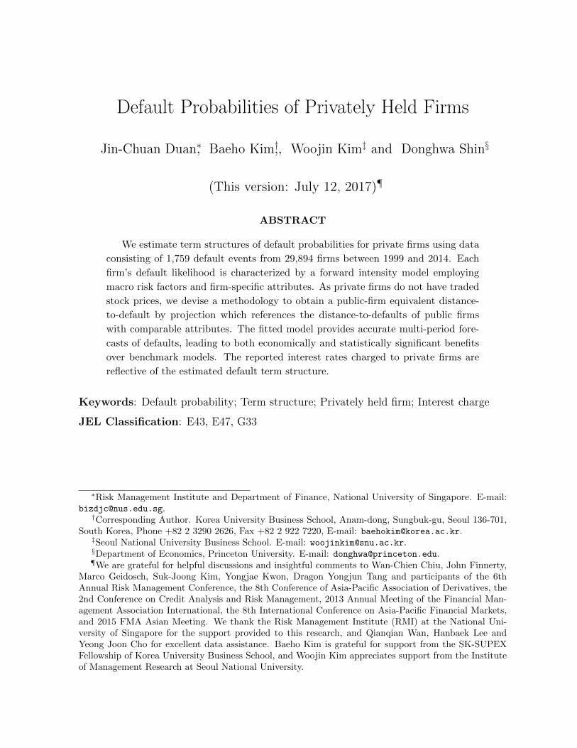
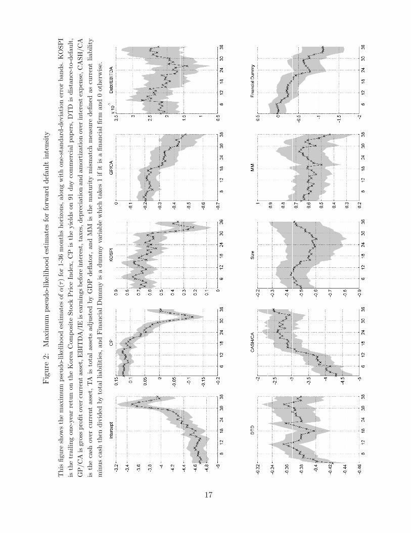
intensity model. Figure 2 reports the maximum pseudo-likelihood estimates for α(τ)
in equation (7) with different prediction horizons ranging from 1 month to 36 months.22
The fitted forward default intensities tend to increase with the yields on 91-day commer-
cial paper for prediction horizons shorter than 2.5 years, whereas the coefficients become
negative and lose their significance for longer horizons. This observation is consistent
with the fact that higher interest rates force firms to carry heavier burden to cover in-
terest expenses; however, such an effect seems to fade in the long run. Admittedly, this
21Refer to A for details of the maximum pseudo-likelihood estimation. The numerical experimentsin our analysis were performed based on code written in MATLAB. We are grateful to Tao Wang forproviding the sample codes to implement the pseudo-likelihood estimation of the forward intensity model.Details are available upon request.
22The forward other-exit intensity model should be estimated as well, but we do not report the resulthere. The maximum pseudo-likelihood estimates for β(τ) in (8) are available upon request.
16
Fig
ure
2:M
axim
um
pse
udo-
likel
ihood
esti
mat
esfo
rfo
rwar
dd
efau
ltin
ten
sity
Th
isfi
gure
show
sth
em
axim
um
pse
ud
o-li
keli
hood
esti
mate
sofα
(τ)
for
1-3
6m
onth
sh
ori
zon
s,alo
ng
wit
hon
e-st
an
dard
-dev
iati
on
erro
rb
an
ds.
KO
SP
I
isth
etr
aili
ng
one-
yea
rre
tun
onth
eK
orea
Com
posi
teS
tock
Pri
ceIn
dex
,C
Pis
the
yie
lds
on
91
day
com
mer
cial
pap
ers,
DT
Dis
dis
tan
ce-t
o-d
efau
lt,
GP
/CA
isgr
oss
pro
fit
over
curr
ent
asse
t,E
BIT
DA
/IE
isea
rnin
gs
bef
ore
inte
rest
,ta
xes
,d
epre
ciati
on
an
dam
ort
izati
on
over
inte
rest
exp
ense
,C
AS
H/C
A
isth
eca
shov
ercu
rren
tas
set,
TA
isto
tal
asse
tsad
just
edby
GD
Pd
eflato
r,an
dM
Mis
the
matu
rity
mis
matc
hm
easu
red
efin
edas
curr
ent
liab
ilit
y
min
us
cash
then
div
ided
by
tota
lli
abil
itie
s,an
dF
inan
cial
Du
mm
yis
ad
um
my
vari
ab
lew
hic
hta
kes
1if
itis
afi
nan
cial
firm
an
d0
oth
erw
ise.
17

phenomenon runs counter to the results obtained by Duffie et al. (2007) in that lower
short-term interest rates were used as a policy instrument to boost the economy during
recessions. For Korean private firms, we find that the former effect outweighs the latter,
offsetting each other for longer prediction horizons, along with business cycles.23
Controlling for other covariates, the forward default intensities are estimated to in-
crease in the trailing one-year return of the KOSPI for all prediction horizons considered.
While this observation is certainly counterintuitive the perspective of univariate reason-
ing, Duffie et al. (2007) and Duan et al. (2012) also report the same result for the effect of
the one-year S&P500 index return on the default intensities of the US public firms. This
relationship could be explained by the fact that the KOSPI return is a lagging business
indicator because of its trailing nature in relation to business cycles.
It turns out that a private firm’s profitability signaled by the GP/CA ratio plays a
significant role in the prediction of defaults. This measure was originally proposed by
Hood & Zhang (2007) for predicting private company defaults in Korea. Holding other
covariates fixed, the estimated forward default intensities in our analysis are decreasing
with the ratio of the gross profit over the current asset for almost all prediction horizons.
Similarly, a firm’s debt coverage measured by the Debt/EBITDA ratio is estimated
to significantly increase the forward default intensities across different prediction horizons.
The inclusion of this covariate is also motivated by Hood & Zhang (2007). The positive
sign of the coefficients is consistent with a simple univariate reasoning.
We also confirm that the DTD measure, which can be interpreted as a volatility-
adjusted measure of leverage, is one of the most crucial attributes in distinguishing dis-
tressed firms from others. Although we use a proxy for private firms’ DTDs because we
are unable to observe their stock prices, the result shows that a smaller value of a firm’s
DTD foreshadows a higher default likelihood with a strong statistical significance. To
the best of our knowledge, this is the first study that proposes a way to use public-firm
equivalent DTDs to gauge the default probabilities of privately held firms. Our finding of
its statistical significance in default prediction is consistent with those public-firm studies
as reported in Bharath & Shumway (2008), Duffie et al. (2007), Duan et al. (2012), and
many others.
We find a significantly negative relationship between the fitted forward default in-
tensities and the CASH/CA ratio after controlling for other covariates. This result is
23In the analysis performed by Duan et al. (2012) on the U.S. public firms, the forward default intensitiesare estimated again to decrease with the three-month Treasury bill rate when the prediction horizon isshorter than one year but to increase for longer horizons.
18

consistent with a univariate reasoning, because this attribute is assumed to represent the
degree of a firm’s liquidity to meet its financial obligations in the near term. Note that
Duan et al. (2012) reports a similar estimation result with the CASH/TA ratio, which is
found to be less indicative in our dataset.
The estimated forward default intensity is, ceteris paribus, significantly decreasing
with the firm’s size measured by its inflation-adjusted value of total assets (normalized
by the Korean GDP deflator) for all horizons. Similar results have been reported in the
prior research such as Kocagil & Reyngold (2003), Hood & Zhang (2007), Duffie et al.
(2007), and Duan et al. (2012), among others.
A firm’s maturity mismatch profile is measured by the current liability minus the cash
then divided by the total liabilities. It reflects the tendency of a business to mismatch
its balance sheet in the sense that liabilities exceed assets in the short run and that
medium- and long-term assets dominate the corresponding obligations. Our estimation
results report that the estimated coefficients for this attribute are significantly positive in
the forward default intensity model for all prediction horizons. In particular, the maturity
mismatch profile makes a strong contribution to the characterization of short-term default
likelihood.
Our forward default intensity model contains a financial dummy variable that takes a
value of 1 if the firm is a financial private firm, and 0 otherwise. The estimated coefficients
are found to be negative but statistically significant in the long run, implying that a
financial firm is exposed to a smaller default risk than an otherwise identical non-financial
firm.
4.3. Forecasting accuracy analysis
This section presents our testing results after performing a prediction accuracy analysis
based on the cumulative accuracy profile of the fitted model. The cumulative accuracy
profile, along with the accuracy ratio as its summary statistic, is in practice the most
popular validation technique to evaluate the prediction power of any default risk ranking
system.
For completeness, we briefly review the concept of the cumulative accuracy profile.24
First, we compute the cumulative default probabilities implied by our fitted forward in-
tensity model at a conditioning time point and rank each of the private firms in our
dataset from the riskiest to safest according to the estimated cumulative default proba-
24A detailed explanation of the cumulative accuracy profile can be found in Vassalou & Xing (2004).
19

Figure 3: Out-of-sample Cumulative Accuracy Profiles
This figure shows the out-of-sample cumulative accuracy profiles based on all private firms in our dataset
from Dec 1999 to Jun 2011 for different modeling approaches for one-year (left panel) and three-year
(right panel) prediction ahead. The fitted logit and probit models share the same risk factors with the
forward intensity model.
0 0.2 0.4 0.6 0.8 10
0.1
0.2
0.3
0.4
0.5
0.6
0.7
0.8
0.9
1
Forward IntensityLogit ModelProbit ModelAltman’s Z−score
0 0.2 0.4 0.6 0.8 10
0.1
0.2
0.3
0.4
0.5
0.6
0.7
0.8
0.9
1
Forward IntensityLogit ModelProbit ModelAltman’s Z−score
bilities. Then, for a given fraction x of the total number of private firms ordered by their
respective risk scores (i.e., default probabilities), we generate a curve by calculating the
percentage of the defaulters whose risk score is equal to or smaller than the maximum
score of each fraction x, ranging from 0 to 1. At the same time, we construct the same
type of curve with a hypothetically perfect rating model, which generates a curve that
increases linearly and then holds constant at one if the fraction x is equal to or larger than
the proportion of firms that default over the risk horizon. Finally, we consider a random
model without any prediction power, which generates a linear curve from 0 to 1 with a
slope of 45. The accuracy ratio is defined as the ratio of the area between the curve of
the model being tested and that of the random model over the area between the curve of
the perfect model and that of the random model. The better the prediction power of a
tested model, the larger the value of its accuracy ratio with the ideal value being one.
We conduct an out-of-sample analysis in the time dimension using a moving-window
approach. Specifically, we re-estimate the model at each month-end from January 2004
with all the data available up to that time and compute the out-of-sample accuracy ratio
over different future periods. That is, the left-hand side of window moves from January
2004 to June 2011 and we use the default data from July 2011 and thereafter for the
out-of-sample validation. By doing so, we fully utilize the historical default data up to
June 2014 for out-of-sample analysis with three years of prediction horizon.
Figure 3 plots the out-of-sample cumulative accuracy profiles of the fitted forward
20

Table 3: Out-of-sample Accuracy Ratios
This table reports the out-sample accuracy ratios based on all private firms in our dataset from December
1999 to June 2014 for different modeling approaches for the prediction horizons of 1 year, 2 years and
3 years, respectively. The fitted logit and probit models share the same risk factors with the forward
intensity model. The 95 percent confidence intervals are calculated based on DeLong, DeLong & Clarke-
Pearson (1988). The Z-statistics are calculated by dividing the difference between two correlated accuracy
ratios of forward intensity model and each of benchmark models (ARforward intensity−ARbenchmark) by the
standard error of the difference following the method of DeLong et al. (1988), where p-values represent
the probability that the two accuracy ratios are equal given the same sample data.Forward Intensity Logit Model Probit Model Altman’s Z-score
1 year
Accuracy Ratio 0.5569 0.5435 0.5396 0.3051(95% C.I.) (0.5501, 0.5638) (0.5364, 0.5506) (0.5326, 0.5466) (0.2970, 0.3132)Z-statistics − 19.677 24.487 57.147(p-value) (<0.0001) (<0.0001) (<0.0001)
2 years
Accuracy Ratio 0.5465 0.5139 0.5128 0.2877(95% C.I.) (0.5409, 0.5520) (0.5083, 0.5195) (0.5072, 0.5184) (0.2814, 0.2939)Z-statistics − 22.782 23.256 75.774(p-value) (<0.0001) (<0.0001) (<0.0001)
3 years
Accuracy Ratio 0.5359 0.4698 0.4665 0.2638(95% C.I.) (0.5310, 0.5407) (0.4649, 0.4748) (0.4616, 0.4713) (0.2563, 0.2693)Z-statistics − 41.502 43.399 89.700(p-value) (<0.0001) (<0.0001) (<0.0001)
intensity model and other alternative models for one-year (left panel) and three-year
(right panel) prediction horizons for the full sample, where the fitted logit and probit
models share the same risk factors with the forward intensity model.25 Note that the
forward-intensity model differs from Altman (2013)’s Z-score model both in the statistical
method and the set of explanatory variables. In comparison to the binary response models,
the forward-intensity model only differ in the econometric method not the explanatory
variables.
For the one-year ahead prediction, we can see that the fitted forward intensity model
with an accuracy ratio of 0.5569 outperforms the alternatives models: the re-estimated
Altman (2013)’s Z-score model for private firms has an accuracy ratio of 0.3051, and the
two binary response models (logit and probit regressions) with the same set of explana-
tory variables as in the forward-intensity model exhibit accuracy ratios of 0.5435 and
0.5396, respectively. Applying the formal testing methodology proposed by DeLong et al.
(1988), we find that the differences in the accuracy ratios implied by the fitted forward
intensity model and each of benchmark models are statistically significant at the standard
confidence level.26
25When we estimate the binary response models, we deal with other exits as non-default cases.26When the two accuracy ratios are estimated based on tests performed on the same data, statistical
analysis on their differences should take into account the positively correlated nature of the samples. In
21

Furthermore, the fitted forward intensity model still maintains its superiority over
the alternative models for longer horizons. For three-year ahead prediction, the fitted
forward intensity model achieves an accuracy ratio of 0.5359, while the prediction accu-
racy ratios for the binary response models (logit model: 0.4698, probit model: 0.4665)
significantly deteriorate with the same explanatory variables. Table 3 summarizes the
out-of-sample accuracy ratios of the fitted forward intensity model and the alternative
models for different prediction horizons. The result shows that the prediction power of
the fitted forward intensity model does not deteriorate for longer horizons relative to other
modeling approaches.
We evaluate the effectiveness of using the DTD-based approach by comparing the
out-of-sample accuracy ratios between the fitted forward intensity model using the DTD-
based approach (With DTD) and the alternative forward intensity model (Without DTD)
by incorporating all variables that we use in the first and second stages.27
Figure 4 shows the one-standard-deviation error bands (boxes) and the 95 percent
confidence intervals (whiskers) of the out-of-sample accuracy ratios based on the two fitted
forward intensity models for one-year (left panel) and three-year (right panel) prediction
ahead. As shown, the public-firm equivalent DTD variables are significantly helpful to
predict private firms’ default for short-term forecasting horizon. In other words, the
alternative one-step estimation cannot outperform our proposed two-step approach, even
if the deviation becomes less pronounced as we increase the forecasting horizon.28 Figure 5
shows the time-series behavior of the estimated median default probabilities in our sample
with risk horizons ranging from 1 month to 36 months. We can observe the economic
vulnerability caused by the global financial crisis of 2008-2009.
Figure 6 illustrates the contribution of each firm-specific attribute to the out-of-
sample prediction power for the fitted forward intensity model. Specifically, we compare
two out-of-sample accuracy ratios of the original forward intensity model (full model) and
Table 3, the Z-statistics are calculated by dividing the difference between two correlated accuracy ratiosby the standard error of the difference following the method of DeLong et al. (1988), where p-valuesrepresent the probability that the two accuracy ratios are equal given the same sample data after takingpossible correlation into account.
27Note that there exists a discrepancy in the determinants of DTD between financial and non-financialfirms. We incorporate a union set of these determinants in the one-step estimation approach, where the‘Interest Expense / Operating Income’ variable, which is available for non-financial firms only, is replacedby the ‘Non-operating Expense / Operating Income’ for financial firms. In this sense, the comparisontest takes a conservative perspective by penalizing the two-step approach, as the alternative one-stepapproach utilizes a larger firm-specific information set.
28According to DeLong et al. (1988), the standardized Z-statistics of the difference in the accuracyratios are 11.6370 (p-value < 0.0001) for 1-year horizon and 1.5771 (p-value = 0.1148) for 3-year predictionahead, respectively.
22

Figure 4: The effectiveness of using the DTD-based approach
This figure compares the out-of-sample accuracy ratios between the fitted forward intensity model using
the DTD-based approach (With DTD) and the alternative forward intensity model (Without DTD)
by incorporating all variables that we use in the first and second stages. The box plots indicate the
one-standard-deviation error bands (boxes) and the 95 percent confidence intervals (whiskers) of the
out-of-sample accuracy ratios based on the fitted forward intensity models for one-year (left panel) and
three-year (right panel) prediction ahead.
With DTD Without DTD0.53
0.535
0.54
0.545
0.55
0.555
0.56
0.5651−year Horizon
With DTD Without DTD0.529
0.531
0.533
0.535
0.537
0.539
0.5413−year Horizon
a benchmark model, both evaluated at their respective maximum likelihood estimators,
where the alternative specification does not include each of the selected firm-specific at-
tribute. Then, we obtain the contribution ratio by dividing the difference between the
two accuracy ratios by the accuracy ratio of the full model. It is remarkable that none of
other firm-specific attributes contribute to the out-of-sample forecasting power of the for-
ward intensity model above and beyond the public-firm equivalent DTD across different
prediction horizons.
Overall, considering the lack of available data for private firms, the prediction power
of the forward intensity model is impressive, not to mention its ability to perform dynamic
estimation over multiple future periods.
4.4. Relationship between interest charge and default risk
Having estimated the term structure of default probabilities for our sample of private firms
based on the forward intensity model, we investigate whether the reported interest rates
of our sample firms actually reflect the credit risk captured by the estimated default term
structure. Specifically, we regress the risk premium, defined as the differencial between
the interest rate on outstanding debts for each firm-year and the risk-free rate, on the
fitted default probability, controlling for other potential factors.
23

Figure 5: Fitted term structures of median default probabilities
This figure shows the time-series behavior of the estimated median default probabilities in our sample
with risk horizons ranging from 1 month to 36 months for conditioning times varying monthly between
January 2004 and June 2011.
2004 2005 2006 2007 2008 2009 2010 2011
06
1218
2430
360
0.005
0.01
0.015
0.02
0.025
0.03
0.035
Year
Horizon (Months)
Def
ault
Pro
babi
lity
For this analysis, interest rate is defined as the weighted average of interest rates.
The risk-free interest rate is estimated for each maturity τ using the standard cubic spline
interpolation from the yields of 91-day certificate of deposit and Korean Governments
Bonds for multiple maturities of 1, 3 and 5 years, obtained from the Economics Statistics
System (ECOS) of the Bank of Korea. Term spread is defined as the yield differential
between the 5-year Korean Government Bonds and the 91-day certificate of deposit. We
define credit spread as the difference between the three-year yield on the corporate bond
issued by AA- rated Korean firms from ECOS and the government bond yield of the same
maturity. Default probability is calculated from the fitted forward intensities by applying
equation (6) for a particular maturity τ . We consider its annualized value, 1τpit(τ), making
it directly compatible with the annualized interest rate. To consider other factors that
may be relevant to the value-weighted interest rate across firms and over time, we include
collateral-to-debt ratio, term spread, credit spread, industry dummies, and several firm
characteristics that significantly affect interest rates.29 In the following analysis we exclude
29As the selected set of firm-specific control variables, we employ the ratio of cash over total assets, theratio of net income over total assets, the ratio of retained earnings over total assets, current assets lesscurrent liabilities then divided by total assets, the ratio of sales over total assets, earnings before interest,taxes, depreciation and amortization divided by total assets, the ratio of gross profit over current assets,total asset sizes, and the maturity mismatch ratio defined as current liability minus cash then divided bytotal liabilities. We exclude the estimated firm-level DTD from this analysis because of multicollinearity
24

Figure 6: Contribution of Firm-specific Attributes to Out-of-sample Accuracy Ratios
This figure shows the contribution ratio of each firm-specific attribute to the out-of-sample prediction
power of the fitted forward intensity model. Contribution ratio is measured as the ratio of the difference
between two accuracy ratios of the original forward intensity model (full model) and an alternative
specification that does not include the selected firm-specific attribute, both evaluated at their respective
maximum likelihood estimators, over the accuracy ratio of the full model.
0 1 2 3 4 5 6 7 8 9 10
GP/CA
DEBT/EBITDA
DTD
CASH/CA
TA
MM
Contribution to Out−of−sample Accuracy Ratio (%)
1 Year2 Years3 Years
all firm-years where the value-weighted interest rate is smaller than the risk-free interest
rate of the same maturity.30 Furthermore, all variables (except for dummy variables)
are winsorized at the first and 99th percentiles to ensure that the results are not unduly
influenced by outliers.
Table 4 provides summary statistics for all the variables after the winsorization (Panel
A) and the results of regressing risk premium on the explanatory variables (Panel B).
The numbers in Panel A of Table 4 indicate that our sample private firms pay roughly
2.37% per annum on their debt instruments over the risk-free rate. Annualized default
probabilities are somewhere around 1.07% on average. The average collateral-to-debt
ratio is roughly 1.12, while the average estimated maturity is 1.78 years. Average term
spread is approximately 0.97% point, while the credit spread is around 1.1% point on
with the fitted default probability and other selected firm-specific attributes. We have also consideredother variables, including the regional dummies and the year dummies, but regional dummies do not showany impact on interest rates while year dummies have confounding effects with the macro level interestrates.
30These are likely to reflect government subsidized loans to small and medium size firms. The fundsare originally provided by government budget, while intermediaries bear all credit risk. Interest rates forthese loans are pre-determined by government policy.
25

average. The negative minimum term spread suggests that there is sometimes a reversal
in yield curve in the Korean debt market. Panel B of Table 4 summarizes the regression
results where the risk premium, which is the difference between the value-weighted interest
rate and the risk-free rate, is the dependent variable and the independent variables are
the fitted default probability, collateral-to-debt ratio, estimated time to maturity, term
spread, credit spread, industry dummy variables, and the selected firm-specific attributes.
To check robustness, we also run similar regressions with firm fixed effects (after excluding
industry dummies and firm-specific attributes) to eliminate time-invariant unobserved
heterogeneity across private firms.
The results clearly indicate that the fitted default probability is a strong predictor of
the risk premium to be charged across different regression specifications. The estimates
are not only statistically significant, but also economically substantial. For example,
the fitted full models (both 4 and 5) suggest that a one standard deviation increase in
default probability leads to 0.24 to 0.31% point increase in risk premium for our sample
private firms after controlling for other variables. These numbers suggest that our forward
intensity model is a useful tool in determining appropriate interest rates charged to private
firms in Korea, and that creditors indeed factor in default probabilities in setting interest
charges.
The shape of interest-rate term structure inferred from the relationship between the
interest rate and the maturity variable seems non-standard. In a standard context, both
default-free interest rates and the yields of high-rated corporate bonds tend to go up as
the time to maturity increases, a pattern commonly known as the normal yield curve. In
contrast, our results based on the universe of Korean private firms show a highly nonlinear
shape of term structure. The estimated term structure shows a significantly downward
sloping term structure for shorter maturities, but the slope becomes positive for longer
than 3.58 to 5.18 years of remaining time to maturity. Our seemingly abnormal finding
suggests that there exists significant roll-over risk premium in the commercial lending
market for private firms, as a firm is exposed by short-term debt to roll-over risk of not
being able to settle its maturing debt. If a firm is subject to a substantial roll-over risk
for its shorter value-weighted maturity, the lender may charge a higher interest rate at
the time of additional loan origination.31 However, such an effect tends to disappear as
31This observation is consistent with the finding of Gopalan, Song & Yerramilli (2014) in that bondmarket investors require premia for taking roll-over risk arising from a firm’s debt maturity structure,and the effects are even stronger among firms with a speculative grade rating. Moreover, poorly-ratedfirms are usually eligible only for short-term high-yield loans, whereas their highly-rated counterparts aremore likely to be granted longer-term borrowings and allowed to pay lower interest charges.
26

the firm’s quality becomes sufficiently high for long-term borrowings.32
As shown, the collateral-to-debt ratio is negatively associated with the risk premium
across different model specifications. The rationale behind this relationship is that com-
mercial lenders tend to lower interest charges when the debt is secured by collaterals
to guarantee a higher recovery rate at default, though the estimated coefficient loses its
significance when firm fixed effects are included in the specification. Ceteris paribus, we
find a significantly positive relationship between risk premium and term spread. This
result is consistent with univariate reasoning, as the term spread measures excess pre-
mium that investors require to commit to holding a long-term bond instead of a series of
otherwise identical shorter-term bonds. As expected, risk premium significantly increases
with market-wide credit risk premium. An increase in credit spread implies that private
firms with higher default probabilities are willing to borrow with a higher interest rate,
reflecting a higher market-wide credit risk premium. Overall, the results suggest that de-
fault probabilities obtained through the forward intensity model is a significant statistic
that explains the observed risk premium charged to private firms in excess of the risk-free
rate.
4.5. Economic benefit of the increased accuracy
We further investigate the economic benefit of adopting our proposed forward intensityapproach over the selected benchmarks.33 Motivated by Stein & Jordao (2003) and Stein(2005), we suppose that banks set a level of lending cut-off (= x) in order to minimizethe cost function (CS) given by
CS(x) = p(D) [c(FN)[1− CAP (x)]− b(TP )CAP (x)] + [1− p(D)] [c(FP )x− b(TN)(1− x)] , (9)
where p(D) is unconditional probability distribution of defaulters in the population of our
sample, b(·) is the benefit of a correct prediction (True Positive or True Negative), c(·) is
the cost of a specific type of error (False Positive or False Negative), and CAP (x) is the
value of cumulative accuracy profile associated with the respective risk score of x ∈ (0, 1).
The first order condition by differentiating CS(x) with respect to x gives the slope of a
line with marginal cost equal to zero, or equivalently, the iso-performance line with slope
S given by
S =1− p(D)
p(D)· c(FP ) + b(TN)
c(FN) + b(TP )(10)
32Similarly, Diamond (1991) also reports a non-linear relationship between debt maturity structure forborrowers and their future credit ratings. Specifically, borrowers with high and low credit ratings aremore likely to issue short-term debt as compared to firms in the middle of the credit quality spectrum.
33We thank an anonymous referee for raising the issue and pointing out the direction of the analysis.
27

Table 4: Regression of the interest rates charged to private firms on default probabilities
Panel A reports summary statistics for the sample used in the regressions and Panel B reports the results of interest rateregressions. The risk premium is the difference between the interest rate and the risk-free rate. The interest rate is theweighted average of interest rates on outstanding debts for each firm-year. Risk-free rate is estimated for each maturityusing the cubic spline interpolation from the yields of 91-day certificate of deposit and Korean Governments Bonds formultiple maturities of 1, 3 and 5 years. Default probability is the annualized value of equation (6) obtained from thefitted forward intensities. Maturity is the value-weighted average of the associated maturities for each debt class, wherethe weights are the relative proportions of each debt class of the estimated maturity for that firm year. Maturity2 is thequadratic term of the Maturity. Collateral-to-debt ratio is the sum of maximum credit amounts of the collaterals scaledby the sum of long-term borrowing, short-term borrowing, current portion of long-term debt and corporate bonds. Termspread is the yield differential between the 5-year Korean Government Bonds and the 91-day certificate of deposit. Creditspread is the difference between the three-year yield on the corporate bond issued by AA- rated Korean firms and thegovernment bond yield of the same maturity. Firm characteristics are the ratio of cash over total assets, the ratio of netincome over total assets, the ratio of retained earnings over total assets, current assets less current liabilities then dividedby total assets, the ratio of sales over total assets, earnings before interest, taxes, depreciation and amortization divided bytotal assets, the ratio of gross profit over current assets, total assets adjusted by GDP inflator, and current liability minuscash then divided by total liabilities. Firm fixed effects denote whether firm fixed effects are included in the specification.A constant is included in each specification but not reported in the table. The t-statistics are presented in parentheses andare computed using heteroscedasticity-robust standard errors, clustered by both firm and year. (*** significant at 1% level,** significant at 5% level, * significant at 10% level)
Panel A: Summary Statistics
Mean Std. Dev Min Median Max
Risk premium 0.0237 0.0161 0.0006 0.0206 0.0743Default probability 0.0107 0.0088 0.0001 0.0087 0.0459Maturity 1.7835 1.2253 0.5063 1.4324 5.7000Collateral-to-debt ratio 1.1197 0.9480 0.0153 0.9577 6.7928Term spread 0.0097 0.0077 -0.0012 0.0078 0.0204Credit spread 0.0109 0.0073 0.0037 0.0098 0.0245
Panel B: Regressions
Dependent variable: Risk premiumModel 1 Model 2 Model 3 Model 4 Model 5
Default probability0.9722*** 0.9548*** 0.3530*** 0.2725***(6.6763) (6.6104) (9.2051) (5.4258)
Maturity-0.0063*** -0.0057*** -0.0064*** -0.0051***(-6.3904) (-5.2321) (-5.9007) (-6.6772)
Maturity2 0.0008*** 0.0008*** 0.0008*** 0.0005***(6.0820) (4.2467) (8.0002) (6.8202)
Collateral-to-debt ratio-0.0007*** -0.0004*** -0.0006*** -0.0001(-3.4804) (-2.7330) (-3.2849) (-0.9051)
Term spread0.4732*** 0.5633***(5.1991) (4.0258)
Credit spread0.4958*** 0.5345**(4.2237) (3.3313)
Firm characteristics Yes Yes Yes Yes NoIndustry dummy Yes Yes Yes Yes NoFirm fixed effects No No No No Yes
Number of obs. 28,717 28,717 28,717 28,717 28,717
Adjusted R2 0.3127 0.1999 0.3261 0.4511 0.7282
28

Table 5: Assumptions for baseline underwriting costs and profits
This table provides the assumed costs and profits for underwriting to a typical client of a bank as a
baseline case scenario. The first row shows the assumed baseline probability of default in the population.
The second and third rows indicate the fees and revenue the bank will generate by making a loan,
respectively. The fourth and fifth rows represent the costs associated with a default. The sixth row is
the median value of the yields of 1-year Korean Governments Bond in the sample period. The last row
shows the average loan amount to small and medium business companies per bank as of December 2015.
All costs and profits are quoted as percentages of a dollar loaned.Variable Value Source
p(D) 5.88% (# of default observation)/(# of firms in the sample)Interest spread (per annum) 2.06% Median of (interest rate − risk-free rate) in the sampleUnderwriting fees (up front) 0.50% Refer to Table 1 of Stein (2005)
Workout fees (on default) 2.00% Refer to Table 1 of Stein (2005)Loss given default 35.0% A report by Korea Institute of Finance (2007)
Risk-free rate (per annum) 4.15% Median of the yields of 1-year Korean Governments Bond
b(TN) 2.56% Interest spread + Underwriting feesc(FN) 35.03% (Workout fees + Loss given default) / (1 + Risk-free rate)
b(TP) = c(FP) 0.00% Refer to Appendix A of Stein (2005)
Annual new loan origination to SMEs $200.0B Estimated by the Financial Services Commission (2013-14)
forms a tangent to the CAP curve at the optimal lending cut-off x∗.
Guided by the baseline case scenario in Appendix A of Stein (2005), we assume
the baseline underwriting costs and profits as reported in Table 5 to calculate the slope
of iso-performance line (10). We further assume for tractability that the lending banks
grant loans that mature in one year, making one payment at the maturity date and that
defaulting firms default at maturity without paying accrued interest.
Figure 7 shows the estimated economic benefit of using the forward intensity model
over alternative models. As shown, the economic benefit of adopting the forward intensity
model with the public-firm equivalent DTD approach is significant, as it would generate
additional profits on the order of about $902.22 million per year over the Altman’s Z-
score model, an easy-to-calculate assessment of a private firm’s financial distress as a
benchmark. Notice that the economic benefit is about 67.95% of the total expected
annual profit of lending based on the Altman’s Z-score model. The economic benefit
of adopting the proposed approach over the Logit model amounts to $94.15 million per
year (which is about 4.41% of the Logit-based expected annual profit), $114.67 million per
year over the Probit model (about 5.42% of the Probit-based expected annual profit). The
economic benefit of adopting the forward intensity model with the public-firm equivalent
DTD approach amounts to $185.47 million per year over the alternative forward intensity
model without DTD by incorporating all variables that we use in the first and second
stages; this extra benefit is approximately 9.07% of the total expected annual profit from
adopting the forward intensity model without the projected DTD variable. This empirical
29

Figure 7: Economic benefit of adopting forward intensity model over alternatives
This figure illustrates the estimated annual economic benefit of adopting the forward intensity model
over alternative models based on the assumptions in Table 5. The numbers are quoted in million US
dollars.
902.22
94.15114.67
185.47
1.00
10.00
100.00
1000.00
Altman's Z-score Model Logit Model Probit Model Forward Intensity Model w/o DTD
finding implies that utilizing forward intensity to model credit behaviors can meaningfully
contribute to credit risk management for privately held firms in Korea as well as for their
creditors.
5. Conclusion
This paper proposes a methodology for estimating default term structure for private firms.
To the best of our knowledge, this is the first study to investigate the dynamic behavior
of default risk for private firms over different future horizons. Our analysis is feasible
due to the unique Korean regulatory environment which requires even private firms to
file their audited financial statements once they exceed a certain size threshold. From
the commercial lenders’ perspective, the proposed framework can be readily applied in
practice to help make credit decisions related to privately held firms.
We adopt a forward-intensity model to characterize multiperiod default likelihoods
using two macro risk factors, six firm-specific attributes, and one dummy variable to dis-
tinguish financial from non-financial firms. The forward-intensity model is calibrated via
maximizing an overlapped pseudo-likelihood. Our out-of-sample test results indicate that
the prediction power of the fitted forward-intensity model is superior to other alternative
models considered, especially for longer prediction horizons.
30

This study provides a better understanding of the lending practice in granting private
firm loans, which constitutes a vital segment of the economy. With the default term
structure in place, we are able to examine whether the interest rates charged to private
firms are positively related to their default risks. The results are consistent with the
notion that default risk is priced in credit contracts and gets manifested in higher interest
rates. We confirm that the economic benefit of adopting our proposed approach over the
use of alternatives is substantial. Our findings suggest that mandating public disclosure
of certain financial information, even for private firms, may facilitate better information
flow between lenders and creditors which could ultimately lead to a more efficient pricing
of credit instruments. An interesting direction for future research would be to explicitly
incorporate possible frailty – unobservable explanatory variables that may be correlated
across firms – and how this may affect the computation and accuracy of private firm
default estimation.
References
Adrian, Tobias & Markus K. Brunnermeier (2016), ‘CoVaR’, American Economic Review
106(7), 1705–1741.
Altman, Edward I. (1968), ‘Financial ratios, discriminant analysis and the prediction of
corporate bankruptcy’, Journal of Finance 23(4), 589–609.
Altman, Edward I. (2013), Predicting financial distress of companies: revisiting the Z-
score and Zeta models, Chapter 17 in Handbook of Research Methods and Applica-
tions in Empirical Finance, UK.
Azizpour, S., K. Giesecke & B Kim (2011), ‘Premia for correlated default risk’, Journal
of Economic Dynamics and Control 35(8), 1340–1357.
Beaver, William H. (1966), ‘Financial ratios as predictors of failure’, Journal of Accounting
Research 4, 71–111.
Bharath, Sreedhar T. & Tyler Shumway (2008), ‘Forecasting default with the merton
distance to default model’, Review of Financial Studies 21(3), 1339–1369.
Campbell, J., J. Hilscher & J. Szilagyi (2008), ‘In search of distress risk’, Journal of
Finance 63(6), 2899–2939.
31

Cangemi, B., De A. Servigny & C. Friedman (2003), Standard and Poor’s credit risk
tracker for private firms technical document. Working Paper, Standard and Poors.
Chava, S. & R. Jarrow (2004), ‘Bankruptcy prediction with industry effects’, Review of
Finance 8(4), 537–569.
DeLong, Elisabeth R., David M. DeLong & Daniel L. Clarke-Pearson (1988), ‘Comparing
the areas under two or more correlated receiver operating characteristic curves: a
nonparametric approach’, Biometrics 44, 837–845.
Diamond, Douglas W. (1991), ‘Debt maturity structure and liquidity risk’, Quarterly
Journal of Economics 106(3), 709–737.
Driessen, J. (2005), ‘Is default event risk priced in corporate bonds?’, Review of Financial
Studies 18(1), 165–195.
Duan, J.-C., J. Sun & T. Wang (2012), ‘Multiperiod corporate default prediction – a
forward intensity approach’, Journal of Econometrics 170(1), 191–209.
Duan, J.-C. & T. Wang (2012), ‘Measuring distance-to-default for financial and non-
financial firms’, Global Credit Review 2(1), 95–108.
Duffie, Darrell & Kenneth J. Singleton (1999), ‘Modeling term structures of defaultable
bonds’, Review of Financial Studies 12(4), 687–720.
Duffie, Darrell, Leandro Saita & Ke Wang (2007), ‘Multi-period corporate default predic-
tion with stochastic covariates’, Journal of Financial Economics 83(3), 635–665.
Falkenstein, E., A. Boral & L.V. Carty (2000), RiskCalcTM for private companies:
Moody’s default model. Working Paper, Moody’s Rating Methodology.
Gopalan, Radhakrishnan, Fenghua Song & Vijay Yerramilli (2014), ‘Debt maturity struc-
ture and credit quality’, Journal of Financial and Quantitative Analysis 49(4), 817–
842.
Hillegeist, S.A., E.K. Keating & D.P. Cram (2004), ‘Assessing the probability of
bankruptcy’, Review of Accounting Studies 9(1), 5–34.
Hood, Frederick & Xiongfei Zhang (2007), ‘Moody’s KMV RiskCalcTM v3.1 Korea’,
Moody’s KMV Company .
Jarrow, R.A., D. Lando & F. Yu (2005), ‘Default risk and diversification: theory and
applications’, Mathematical Finance 15(1), 1–26.
32

Kocagil, Ahment E. & Alexander Reyngold (2003), ‘Moody’s RiskCalcTM for private
companies: Korea’, Moody’s Rating Methodology .
Merton, R.C. (1974), ‘On the pricing of corporate debt: The risk structure of interest
rates’, Journal of Finance 29(2), 449–470.
Ohlson, J.A. (1980), ‘Financial ratios and the probabilistic prediction of bankruptcy’,
Journal of Accounting Research 18(1), 109–131.
Pan, J. & K. Singleton (2008), ‘Default and recovery implicit in the term structure of
sovereign CDS spreads’, Journal of Finance 63(5), 23452384.
Pittman, Jeffery A. & Steve Foretin (2004), ‘Auditor choice and the cost of debt capital
for newly public firms’, Journal of Accounting and Economics 37(1), 113–136.
Protter, Philip (2004), Stochastic Integration and Differential Equations, Springer-Verlag,
New York.
Stein, Roger M. (2005), ‘The relationship between default prediction and lending prof-
its: Integrating ROC analysis and loan pricing’, Journal of Banking and Finance
29, 1213–1236.
Stein, Roger M. & Felipe Jordao (2003), What is a more powerful model worth? Moody’s
KMV Technical Report #030124.
Vassalou, M. & Y. H. Xing (2004), ‘Default risk in equity returns’, Journal of Finance
59(2), 831–868.
A. Overlapped pseudo-likelihood function
This appendix provides an outline of our model calibration scheme based on forward
intensities. Sample period is from 0 to T over monthly time grid. Using the notations in
Section 2, the pseudo-likelihood function for prediction horizon τ measured in months with
each equal to ∆t (= 1 month) can be expressed under the doubly stochastic assumption
(also known as conditional independence assumption) as
Lτ (α, β; τC , τD, X) =N∏i=1
dT/∆te−1∏k=0
Liτ,k∆t(α, β; τ iC , τiD, X
i), (11)
33

where α = α(0), . . . , α(τ − 1), β = β(0), . . . , β(τ − 1), τC =τ 1C , . . . , τ
NC
, τD =
τ 1D, . . . , τ
ND
, X =
X1, . . . , XN
, and
Liτ,t(α, β; τ iC , τiD, X
i) = 1ti0≤t, τ iC>t+τLt(τ iC ; τ iC > t+ τ
)+ 1ti0≤t<τ iC≤t+τ, τ iD=τ iCLt
(τ iC ; τ iC ≤ t+ τ, τ iD = τ iC
)+ 1ti0≤t<τ iC≤t+τ, τ iD 6=τ iCLt
(τ iC ; τ iC ≤ t+ τ, τ iD 6= τ iC
)+ 1ti0>t + 1τ iC≤t, (12)
where ti0 is the first month that it appeared in the data set, and the parameters α and β
characterize the forward default intensity f it (τ) and forward other exit intensity git(τ) −f it (τ), respectively. The first term on the right-hand side of (12) refers to the likelihood
of surviving both forms of exit. The second term represents the likelihood that the i-th
firm defaults at a particular time point. The third term is the likelihood that the firm
exits due to other reasons. If the firm does not appear in the sample in month t as shown
in the last two terms, we set the pseudo-likelihood to 1, which is transformed to 0 in the
logarithm.
The pseudo-likelihood function in (11) can be expressed as the product of separate
terms involving α and β. Thus, we can maximize its two components separately to obtain
the maximum pseudo-likelihood estimates.34 In addition, the pseudo-likelihood function
for α or β can be further decomposed into separate terms involving α(τ) or β(τ) across
different τ ’s. Hence, we can obtain their maximum pseudo-likelihood estimates without
having to perform estimation sequentially from shorter to longer prediction horizons. The
horizon-specific pseudo-likelihood functions are given by
Lαs (α; τC , τD, X) =N∏i=1
d(T−s)/∆te−1∏k=0
Lα,is,k∆t(α(s); τ iC , τiD, X
i) (13)
Lβs (β; τC , τD, X) =N∏i=1
d(T−s)/∆te−1∏k=0
Lβ,is,k∆t(β(s); τ iC , τiD, X
i) (14)
for s = 0,∆t, 2∆t, · · · , τ −∆t as intended prediction horizons measured in months. This
leads to the following expressions in the form of
34Refer to Proposition 2 of Duffie et al. (2007) for similar arguments.
34

Lα,is,t (α(s); τ iC , τiD, X
i) = 1ti0≤t, τ iC>t+∆t+s exp[−f it (s)∆t
]+ 1ti0≤t, τ iD=τ iC=t+∆t+s
(1− exp
[−f it (s)∆t
])+ 1ti0≤t, τ iD 6=τ iC=t+∆t+s exp
[−f it (s)∆t
]+ 1ti0>t + 1τ iC<t+∆t+s, (15)
Lβ,is,t (β(s); τ iC , τiD, X
i) = 1ti0≤t, τ iC>t+∆t+s exp[−hik∆t(s)∆t
]+ 1ti0≤t, τ iD=τ iC=t+∆t+s
+ 1ti0≤t, τ iD 6=τ iC=t+∆t+s(1− exp
[−hik∆t(s)∆t
])+ 1ti0>t + 1τ iC<t+∆t+s, (16)
where hit(τ) = git(τ)− f it (τ) and s = 0,∆t, 2∆t, · · · , τ −∆t.
Note that the pseudo-likelihood function is constructed with observations from over-
lapped periods when the prediction horizon τ is longer than ∆t. Because of the overlapping
nature of the pseudo-likelihood function, the associated inference violates the standard
assumption. In this regard, Duan et al. (2012) characterize and derive the large sample
properties of the estimator based on maximizing the pseudo-likelihood function; see Ap-
pendix A therein. Under mild regularity conditions, they prove its asymptotic consistency
by showing that the difference between the maximum pseudo-likelihood estimator and the
true data-generating parameter converges weakly to a vector whos distribution is joint
normal with mean zero.35
35A more detailed proof of consistency is available upon request.
35
Related Documents