Deeper Understanding, Faster Calc: SOA MFE and CAS Exam 3F Yufeng Guo July 5, 2011

Welcome message from author
This document is posted to help you gain knowledge. Please leave a comment to let me know what you think about it! Share it to your friends and learn new things together.
Transcript

Deeper Understanding, Faster Calc: SOA MFE
and CAS Exam 3F
Yufeng Guo
July 5, 2011

Contents
Introduction ix
9 Parity and other option relationships 1
9.1 Put-call parity . . . . . . . . . . . . . . . . . . . . . . . . . . . . 1
9.1.1 Option on stocks . . . . . . . . . . . . . . . . . . . . . . . 1
9.1.2 Options on currencies . . . . . . . . . . . . . . . . . . . . 11
9.1.3 Options on bonds . . . . . . . . . . . . . . . . . . . . . . . 13
9.1.4 Generalized parity and exchange options . . . . . . . . . . 13
9.1.5 Comparing options with respect to style, maturity, and
strike . . . . . . . . . . . . . . . . . . . . . . . . . . . . . 19
10 Binomial option pricing: I 35
10.1 One-period binomial model: simple examples . . . . . . . . . . . 35
10.2 General one-period binomial model . . . . . . . . . . . . . . . . . 36
10.2.1 Two or more binomial trees . . . . . . . . . . . . . . . . . 49
10.2.2 Options on stock index . . . . . . . . . . . . . . . . . . . 64
10.2.3 Options on currency . . . . . . . . . . . . . . . . . . . . . 67
10.2.4 Options on futures contracts . . . . . . . . . . . . . . . . 71
11 Binomial option pricing: II 79
11.1 Understanding early exercise . . . . . . . . . . . . . . . . . . . . 79
11.2 Understanding risk-neutral probability . . . . . . . . . . . . . . . 80
11.2.1 Pricing an option using real probabilities . . . . . . . . . 81
11.2.2 Binomial tree and lognormality . . . . . . . . . . . . . . . 88
11.2.3 Estimate stock volatility . . . . . . . . . . . . . . . . . . . 91
11.3 Stocks paying discrete dividends . . . . . . . . . . . . . . . . . . 95
11.3.1 Problems with discrete dividend tree . . . . . . . . . . . . 97
11.3.2 Binomial tree using prepaid forward . . . . . . . . . . . . 98
12 Black-Scholes 105
12.1 Introduction to the Black-Scholes formula . . . . . . . . . . . . . 105
12.1.1 Call and put option price . . . . . . . . . . . . . . . . . . 105
12.1.2 When is the Black-Scholes formula valid? . . . . . . . . . 107
12.2 Derive the Black-Scholes formula . . . . . . . . . . . . . . . . . . 107
iii
iv CONTENTS
12.3 Applying the formula to other assets . . . . . . . . . . . . . . . . 121
12.3.1 Black-Scholes formula in terms of prepaid forward price . 121
12.3.2 Options on stocks with discrete dividends . . . . . . . . . 121
12.3.3 Options on currencies . . . . . . . . . . . . . . . . . . . . 122
12.3.4 Options on futures . . . . . . . . . . . . . . . . . . . . . . 123
12.4 Option the Greeks . . . . . . . . . . . . . . . . . . . . . . . . . . 124
12.4.1 Delta . . . . . . . . . . . . . . . . . . . . . . . . . . . . . 124
12.4.2 Gamma . . . . . . . . . . . . . . . . . . . . . . . . . . . . 125
12.4.3 Vega . . . . . . . . . . . . . . . . . . . . . . . . . . . . . . 125
12.4.4 Theta . . . . . . . . . . . . . . . . . . . . . . . . . . . . . 126
12.4.5 Rho . . . . . . . . . . . . . . . . . . . . . . . . . . . . . . 126
12.4.6 Psi . . . . . . . . . . . . . . . . . . . . . . . . . . . . . . . 126
12.4.7 Greek measures for a portfolio . . . . . . . . . . . . . . . 126
12.4.8 Option elasticity and volatility . . . . . . . . . . . . . . . 127
12.4.9 Option risk premium and Sharpe ratio . . . . . . . . . . . 128
12.4.10Elasticity and risk premium of a portfolio . . . . . . . . . 129
12.5 Profit diagrams before maturity . . . . . . . . . . . . . . . . . . . 129
12.5.1 Holding period profit . . . . . . . . . . . . . . . . . . . . . 129
12.5.2 Calendar spread . . . . . . . . . . . . . . . . . . . . . . . 132
12.6 Implied volatility . . . . . . . . . . . . . . . . . . . . . . . . . . . 133
12.6.1 Calculate the implied volatility . . . . . . . . . . . . . . . 133
12.6.2 Volatility skew . . . . . . . . . . . . . . . . . . . . . . . . 134
12.6.3 Using implied volatility . . . . . . . . . . . . . . . . . . . 135
12.7 Perpetual American options . . . . . . . . . . . . . . . . . . . . . 135
12.7.1 Perpetual calls and puts . . . . . . . . . . . . . . . . . . . 135
12.7.2 Barrier present values . . . . . . . . . . . . . . . . . . . . 140
13 Market-making and delta-hedging 143
13.1 Delta hedging . . . . . . . . . . . . . . . . . . . . . . . . . . . . . 143
13.2 Examples of Delta hedging . . . . . . . . . . . . . . . . . . . . . 143
13.3 Textbook Table 13.2 . . . . . . . . . . . . . . . . . . . . . . . . . 152
13.4 Textbook Table 13.3 . . . . . . . . . . . . . . . . . . . . . . . . . 154
13.5 Mathematics of Delta hedging . . . . . . . . . . . . . . . . . . . . 155
13.5.1 Delta-Gamma-Theta approximation . . . . . . . . . . . . 155
13.5.2 Understanding the market maker’s profit . . . . . . . . . 156
14 Exotic options: I 159
14.1 Asian option (i.e. average options) . . . . . . . . . . . . . . . . . 159
14.1.1 Characteristics . . . . . . . . . . . . . . . . . . . . . . . . 159
14.1.2 Examples . . . . . . . . . . . . . . . . . . . . . . . . . . . 160
14.1.3 Geometric average . . . . . . . . . . . . . . . . . . . . . . 160
14.1.4 Payoff at maturity . . . . . . . . . . . . . . . . . . . . . 160
14.2 Barrier option . . . . . . . . . . . . . . . . . . . . . . . . . . . . . 161
14.2.1 Knock-in option . . . . . . . . . . . . . . . . . . . . . . . 161
14.2.2 Knock-out option . . . . . . . . . . . . . . . . . . . . . . . 161
CONTENTS v
14.2.3 Rebate option . . . . . . . . . . . . . . . . . . . . . . . . . 161
14.2.4 Barrier parity . . . . . . . . . . . . . . . . . . . . . . . . . 162
14.2.5 Examples . . . . . . . . . . . . . . . . . . . . . . . . . . . 162
14.3 Compound option . . . . . . . . . . . . . . . . . . . . . . . . . . 163
14.4 Gap option . . . . . . . . . . . . . . . . . . . . . . . . . . . . . . 165
14.4.1 Definition . . . . . . . . . . . . . . . . . . . . . . . . . . . 165
14.4.2 Pricing formula . . . . . . . . . . . . . . . . . . . . . . . . 165
14.4.3 How to memorize the pricing formula . . . . . . . . . . . 165
14.5 Exchange option . . . . . . . . . . . . . . . . . . . . . . . . . . . 166
18 Lognormal distribution 169
18.1 Normal distribution . . . . . . . . . . . . . . . . . . . . . . . . . 169
18.2 Lognormal distribution . . . . . . . . . . . . . . . . . . . . . . . . 170
18.3 Lognormal model of stock prices . . . . . . . . . . . . . . . . . . 170
18.4 Lognormal probability calculation . . . . . . . . . . . . . . . . . . 171
18.4.1 Lognormal confidence interval . . . . . . . . . . . . . . . . 172
18.4.2 Conditional expected prices . . . . . . . . . . . . . . . . . 176
18.4.3 Black-Scholes formula . . . . . . . . . . . . . . . . . . . . 177
18.5 Estimating the parameters of a lognormal distribution . . . . . . 177
18.6 How are asset prices distributed . . . . . . . . . . . . . . . . . . . 179
18.6.1 Histogram . . . . . . . . . . . . . . . . . . . . . . . . . . . 179
18.6.2 Normal probability plots . . . . . . . . . . . . . . . . . . . 180
18.7 Sample problems . . . . . . . . . . . . . . . . . . . . . . . . . . . 182
19 Monte Carlo valuation 187
19.1 Example 1 Estimate () . . . . . . . . . . . . . . . . . . . . . 187
19.2 Example 2 Estimate . . . . . . . . . . . . . . . . . . . . . . . . 191
19.3 Example 3 Estimate the price of European call or put options . . 194
19.4 Example 4 Arithmetic and geometric options . . . . . . . . . . . 198
19.5 Efficient Monte Carlo valuation . . . . . . . . . . . . . . . . . . . 207
19.5.1 Control variance method . . . . . . . . . . . . . . . . . . . 207
19.6 Antithetic variate method . . . . . . . . . . . . . . . . . . . . . . 211
19.7 Stratified sampling . . . . . . . . . . . . . . . . . . . . . . . . . . 213
19.7.1 Importance sampling . . . . . . . . . . . . . . . . . . . . . 213
19.8 Sample problems . . . . . . . . . . . . . . . . . . . . . . . . . . . 213
20 Brownian motion and Ito’s Lemma 219
20.1 Introduction . . . . . . . . . . . . . . . . . . . . . . . . . . . . . . 219
20.1.1 Big picture . . . . . . . . . . . . . . . . . . . . . . . . . . 220
20.2 Brownian motion . . . . . . . . . . . . . . . . . . . . . . . . . . . 221
20.2.1 Deterministic process vs. stochastic process . . . . . . . . 221
20.2.2 Definition of Brownian motion . . . . . . . . . . . . . . . 222
20.2.3 Martingale . . . . . . . . . . . . . . . . . . . . . . . . . . 224
20.2.4 Properties of Brownian motion . . . . . . . . . . . . . . . 231
vi CONTENTS
20.2.5 Arithmetic Brownian motion and Geometric Brownian
motion . . . . . . . . . . . . . . . . . . . . . . . . . . . . . 236
20.2.6 Ornstein-Uhlenbeck process . . . . . . . . . . . . . . . . . 237
20.3 Definition of the stochastic calculus . . . . . . . . . . . . . . . . . 238
20.3.1 Why stochastic calculus . . . . . . . . . . . . . . . . . . . 238
20.4 Properties of the stochastic calculus . . . . . . . . . . . . . . . . 248
20.5 Ito’s lemma . . . . . . . . . . . . . . . . . . . . . . . . . . . . . . 251
20.5.1 Multiplication rules . . . . . . . . . . . . . . . . . . . . . 251
20.5.2 Ito’s lemma . . . . . . . . . . . . . . . . . . . . . . . . . . 252
20.6 Geometric Brownian motion revisited . . . . . . . . . . . . . . . 253
20.6.1 Relative importance of drift and noise term . . . . . . . . 254
20.6.2 Correlated Ito processes . . . . . . . . . . . . . . . . . . . 254
20.7 Three worlds: , , and . . . . . . . . . . . . . . . . . . . . . 261
20.8 Sharpe ratio . . . . . . . . . . . . . . . . . . . . . . . . . . . . . . 305
20.9 Girsanov’s theorem . . . . . . . . . . . . . . . . . . . . . . . . . . 308
20.10Risk neutral process . . . . . . . . . . . . . . . . . . . . . . . . . 317
20.11Valuing a claim on . . . . . . . . . . . . . . . . . . . . . . . . 330
20.11.1Process followed by . . . . . . . . . . . . . . . . . . . . 330
20.11.2Formula for () and E£ ()
¤. . . . . . . . . . . . . . 330
20.11.3Expected return of a claim on () . . . . . . . . . . . . 331
20.11.4Specific examples . . . . . . . . . . . . . . . . . . . . . . . 332
21 Black-Scholes equation 341
21.1 Differential equations and valuation under certainty . . . . . . . 341
21.1.1 Valuation equation . . . . . . . . . . . . . . . . . . . . . . 341
21.1.2 Bonds . . . . . . . . . . . . . . . . . . . . . . . . . . . . . 342
21.1.3 Dividend paying stock . . . . . . . . . . . . . . . . . . . . 342
21.2 Black-Scholes equation . . . . . . . . . . . . . . . . . . . . . . . . 342
21.2.1 How to derive Black-Scholes equation . . . . . . . . . . . 342
21.2.2 Verifying the formula for a derivative . . . . . . . . . . . . 343
21.2.3 Black-Scholes equation and equilibrium returns . . . . . . 346
21.3 Risk-neutral pricing . . . . . . . . . . . . . . . . . . . . . . . . . 348
22 Exotic options: II 349
22.1 All-or-nothing options . . . . . . . . . . . . . . . . . . . . . . . . 349
23 Volatility 351
24 Interest rate models 353
24.1 Market-making and bond pricing . . . . . . . . . . . . . . . . . . 353
24.1.1 Review of duration and convexity . . . . . . . . . . . . . . 353
24.1.2 Interest rate is not so simple . . . . . . . . . . . . . . . . 360
24.1.3 Impossible bond pricing model . . . . . . . . . . . . . . . 361
24.1.4 Equilibrium equation for bonds . . . . . . . . . . . . . . . 365
24.1.5 Delta-Gamma approximation for bonds . . . . . . . . . . 370
24.2 Equilibrium short-rate bond price models . . . . . . . . . . . . . 371
CONTENTS vii
24.2.1 Arithmetic Brownian motion (i.e. Merton model) . . . . . 371
24.2.2 Rendleman-Bartter model . . . . . . . . . . . . . . . . . . 372
24.2.3 Vasicek model . . . . . . . . . . . . . . . . . . . . . . . . 373
24.2.4 CIR model . . . . . . . . . . . . . . . . . . . . . . . . . . 395
24.3 Bond options, caps, and the Black model . . . . . . . . . . . . . 400
24.3.1 Black formula . . . . . . . . . . . . . . . . . . . . . . . . . 400
24.3.2 Interest rate caplet . . . . . . . . . . . . . . . . . . . . . . 403
24.4 Binomial interest rate model . . . . . . . . . . . . . . . . . . . . 404
24.5 Black-Derman-Toy model . . . . . . . . . . . . . . . . . . . . . . 408
Introduction
This study guide is for SOA MFE and CAS Exam 3F. Before you start, make
sure you have the following items:
1. Derivatives Markets, the 2nd edition.
2. Errata of Derivatives Markets. You can download the errata at http://
www.kellogg.northwestern.edu/faculty/mcdonald/htm/typos2e_01.
html. Don’t miss the errata about the textbook pages 780 through 788.
3. Download the syllabus from the SOA or CAS website.
4. Download the sample MFE problems and solutions from the SOA website.
5. Download the recent SOA MFE and CAS Exam 3 problems.
Please report any errors to [email protected].
ix
Chapter 12
Black-Scholes
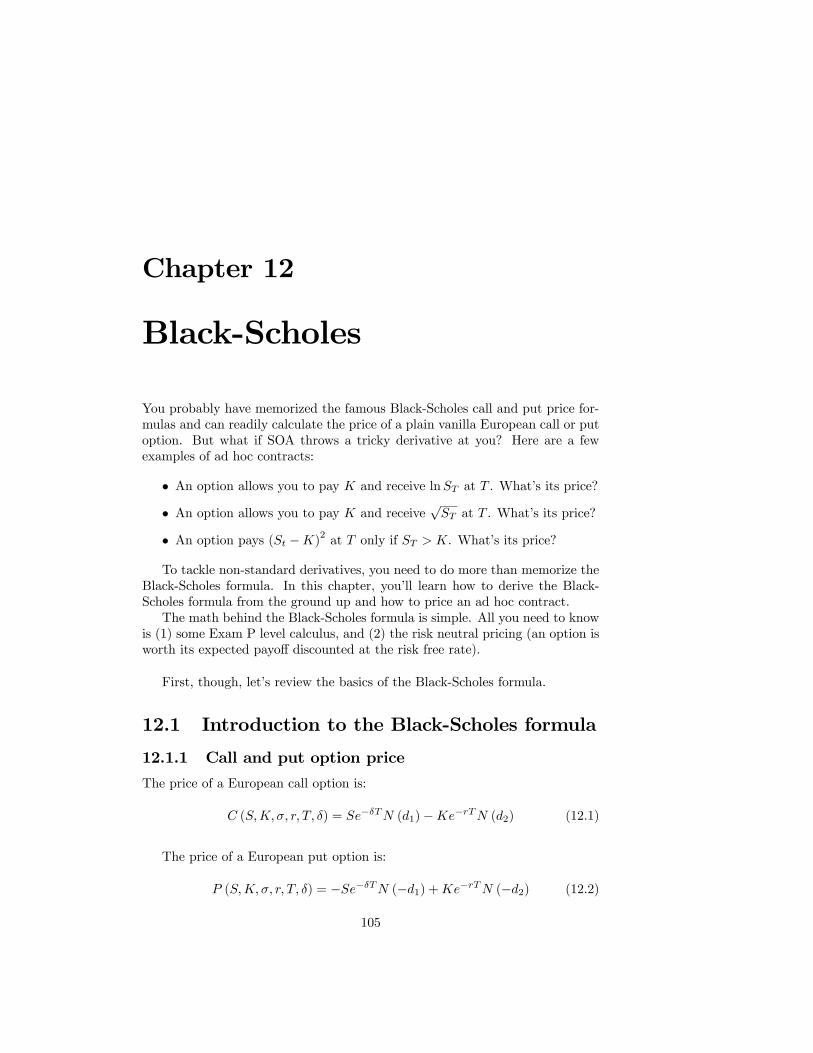
You probably have memorized the famous Black-Scholes call and put price for-
mulas and can readily calculate the price of a plain vanilla European call or put
option. But what if SOA throws a tricky derivative at you? Here are a few
examples of ad hoc contracts:
• An option allows you to pay and receive ln at . What’s its price?
• An option allows you to pay and receive√ at . What’s its price?
• An option pays ( −)2at only if . What’s its price?
To tackle non-standard derivatives, you need to do more than memorize the
Black-Scholes formula. In this chapter, you’ll learn how to derive the Black-
Scholes formula from the ground up and how to price an ad hoc contract.
The math behind the Black-Scholes formula is simple. All you need to know
is (1) some Exam P level calculus, and (2) the risk neutral pricing (an option is
worth its expected payoff discounted at the risk free rate).
First, though, let’s review the basics of the Black-Scholes formula.
12.1 Introduction to the Black-Scholes formula
12.1.1 Call and put option price
The price of a European call option is:
( ) = − (1)−− (2) (12.1)
The price of a European put option is:
( ) = −− (−1) +− (−2) (12.2)
105
106 CHAPTER 12. BLACK-SCHOLES
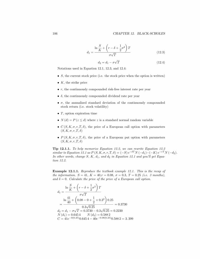
1 =
ln
+
µ − +
1
22
√
(12.3)
2 = 1 − √ (12.4)
Notations used in Equation 12.1, 12.3, and 12.4:
• , the current stock price (i.e. the stock price when the option is written)
• , the strike price
• , the continuously compounded risk-free interest rate per year
• , the continuously compounded dividend rate per year
• , the annualized standard deviation of the continuously compounded
stock return (i.e. stock volatility)
• , option expiration time
• () = ( ≤ ) where is a standard normal random variable
• ( ), the price of a European call option with parameters
( )
• ( ), the price of a European put option with parameters
( )
Tip 12.1.1. To help memorize Equation 12.2, we can rewrite Equation 12.2
similar to Equation 12.1 as ( ) = (−) − (−1)−(−) − (−2).In other words, change , , 1, and 2 in Equation 12.1 and you’ll get Equa-
tion 12.2.
Example 12.1.1. Reproduce the textbook example 12.1. This is the recap of
the information. = 41, = 40, = 008, = 03, = 025 (i.e. 3 months),
and = 0. Calculate the price of the price of a European call option.
1 =
ln
+
µ − +
1
22
√
=
ln41
40+
µ008− 0 + 1
2× 032
¶025
03√025
= 03730
2 = 1 − √ = 03730− 03√025 = 02230
(1) = 0645 4 (2) = 0588 2
= 41−0(025)0645 4− 40−008(025)0588 2 = 3 399

12.2. DERIVE THE BLACK-SCHOLES FORMULA 107
Example 12.1.2. Reproduce the textbook example 12.2. This is the recap of
the information. = 41, = 40, = 008, = 03, = 025 (i.e. 3 months),
and = 0. Calculate the price of the price of a European put option.
(−1) = 1− (1) = 1− 0645 4 = 0354 6 (−2) = 1− (2) = 1− 0588 2 = 0411 8 = −41−0(025)0354 6 + 40−008(025)0411 8 = 1 607
12.1.2 When is the Black-Scholes formula valid?
Assumptions under the Black-Scholes formula:
Assumptions about the distribution of stock price:
1. Continuously compounded returns on the stock are normally distributed
(i.e. stock price is lognormally distributed) and independent over time
2. The volatility of the continuously compounded returns is known and con-
stant
3. Future dividends are known, either as a dollar amount (i.e. and are
known in advance) or as a fixed dividend yield (i.e. is a known constant)
Assumptions about the economic environment
1. The risk-free rate is known and fixed (i.e. is a known constant)
2. There are no transaction costs or taxes
3. It’s possible to short-sell costlessly and to borrow at the risk-free rate
12.2 Derive the Black-Scholes formula
By learning how to derive the Black-Scholes formula, we’ll be able to remove
the black-box behind the formula and recreate the formula instantly. First, some
basics.
What’s the density function of a standard normal random variable?
If ∼ (0 1), then () =1√2
−052
, Φ () = ( ≤ ) =R −∞ ()
How can we convert a normal variable to a standard normal variable?
If ∼ ¡ 2
¢, then set =
−
; = +
What’s the stock price under the Black-Scholes assumption in the real world?
DM 20.13: = 0 exp£¡− − 052¢ +
√¤, ∼ (0 1)
What’s under the Black-Scholes assumption in the risk neutral world ?
Set = . Then = 0 exp
£¡ − − 052¢ +
√¤, ∼ (0 1)
108 CHAPTER 12. BLACK-SCHOLES
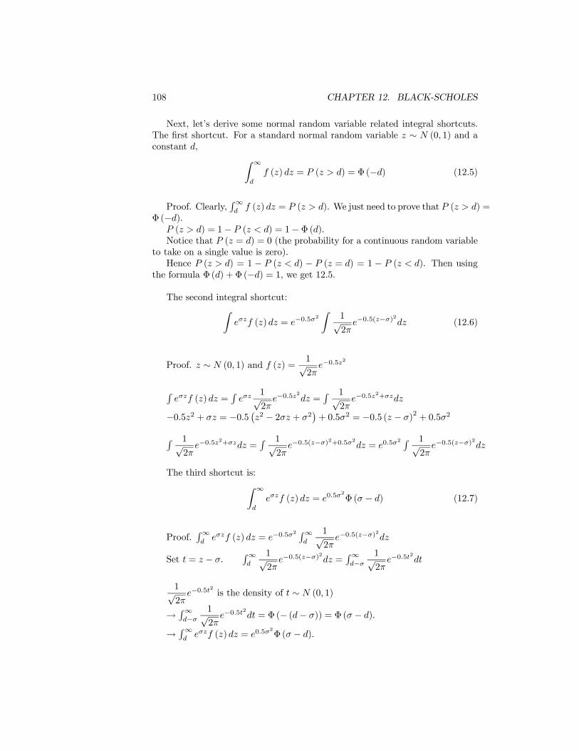
Next, let’s derive some normal random variable related integral shortcuts.
The first shortcut. For a standard normal random variable ∼ (0 1) and a
constant , Z ∞
() = ( ) = Φ (−) (12.5)
Proof. Clearly,R∞
() = ( ). We just need to prove that ( ) =
Φ (−). ( ) = 1− ( ) = 1−Φ ().Notice that ( = ) = 0 (the probability for a continuous random variable
to take on a single value is zero).
Hence ( ) = 1 − ( ) − ( = ) = 1 − ( ). Then using
the formula Φ () +Φ (−) = 1, we get 12.5.
The second integral shortcut:Z () = −05
2
Z1√2
−05(−)2
(12.6)
Proof. ∼ (0 1) and () =1√2
−052
R () =
R
1√2
−052
=R 1√
2−05
2+
−052 + = −05 ¡2 − 2 + 2¢+ 052 = −05 ( − )
2+ 052
R 1√2
−052+ =
R 1√2
−05(−)2+052 = 05
2 R 1√2
−05(−)2
The third shortcut is:Z ∞
() = 052
Φ ( − ) (12.7)
Proof.R∞
() = −052 R∞
1√2
−05(−)2
Set = − .R∞
1√2
−05(−)2
=R∞−
1√2
−052
1√2
−052
is the density of ∼ (0 1)
→ R∞−
1√2
−052
= Φ (− (− )) = Φ ( − ).
→ R∞
() = 052
Φ ( − ).
12.2. DERIVE THE BLACK-SCHOLES FORMULA 109
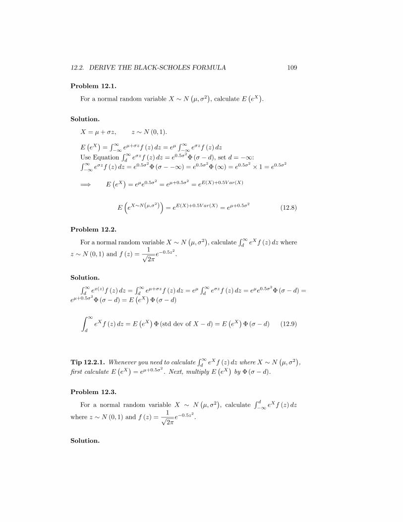
Problem 12.1.
For a normal random variable ∼ ¡ 2
¢, calculate
¡¢.
Solution.
= + , ∼ (0 1).
¡¢=R∞−∞ + () =
R∞−∞ ()
Use EquationR∞
() = 052
Φ ( − ), set = −∞:R∞−∞ () = 05
2
Φ ( −−∞) = 052
Φ (∞) = 052 × 1 = 05
2
=⇒ ¡¢= 05
2
= +052
= ()+05 ()
³∼(
2)´= ()+05 () = +05
2
(12.8)
Problem 12.2.
For a normal random variable ∼ ¡ 2
¢, calculate
R∞
() where
∼ (0 1) and () =1√2
−052
.
Solution.R∞
() () =R∞
+ () = R∞
() = 052
Φ ( − ) =
+052
Φ ( − ) = ¡¢Φ ( − )
Z ∞
() = ¡¢Φ (std dev of − ) =
¡¢Φ ( − ) (12.9)
Tip 12.2.1. Whenever you need to calculateR∞
() where ∼ ¡ 2
¢,
first calculate ¡¢= +05
2
. Next, multiply ¡¢by Φ ( − ).
Problem 12.3.
For a normal random variable ∼ ¡ 2
¢, calculate
R −∞ ()
where ∼ (0 1) and () =1√2
−052
.
Solution.
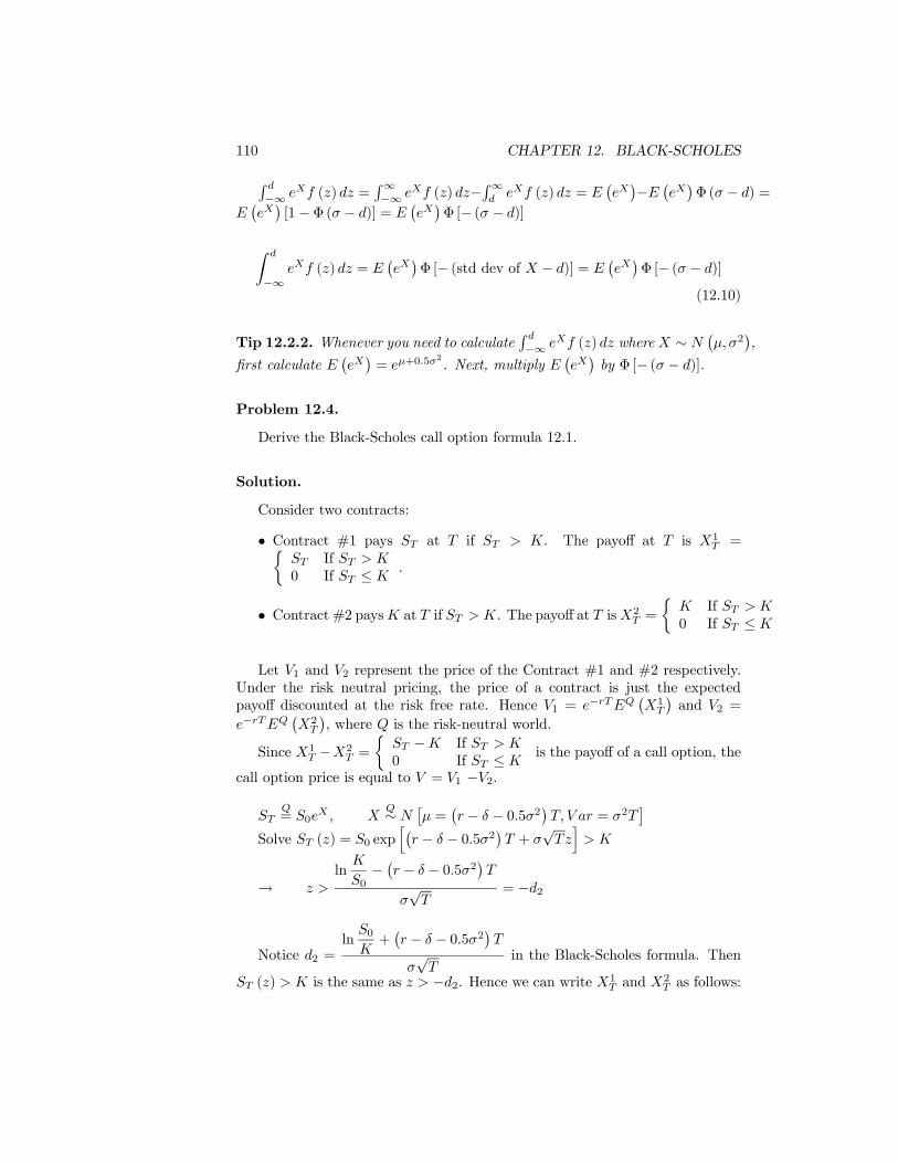
110 CHAPTER 12. BLACK-SCHOLES
R −∞ () =
R∞−∞ () −R∞
() =
¡¢− ¡¢Φ ( − ) =
¡¢[1−Φ ( − )] =
¡¢Φ [− ( − )]
Z
−∞ () =
¡¢Φ [− (std dev of − )] =
¡¢Φ [− ( − )]
(12.10)
Tip 12.2.2. Whenever you need to calculateR −∞ () where ∼
¡ 2
¢,
first calculate ¡¢= +05
2
. Next, multiply ¡¢by Φ [− ( − )].
Problem 12.4.
Derive the Black-Scholes call option formula 12.1.
Solution.
Consider two contracts:
• Contract #1 pays at if . The payoff at is 1 =½
If
0 If ≤ .
• Contract #2 pays at if . The payoff at is2 =
½ If
0 If ≤
Let 1 and 2 represent the price of the Contract #1 and #2 respectively.
Under the risk neutral pricing, the price of a contract is just the expected
payoff discounted at the risk free rate. Hence 1 = −¡1
¢and 2 =
−¡2
¢, where is the risk-neutral world.
Since 1 −2
=
½ − If
0 If ≤ is the payoff of a call option, the
call option price is equal to = 1 −2.
= 0
, ∼
£ =
¡ − − 052¢ = 2
¤Solve () = 0 exp
h¡ − − 052¢ +
√i
→
ln
0− ¡ − − 052¢
√
= −2
Notice 2 =ln
0
+¡ − − 052¢√
in the Black-Scholes formula. Then
() is the same as −2. Hence we can write 1 and
2 as follows:
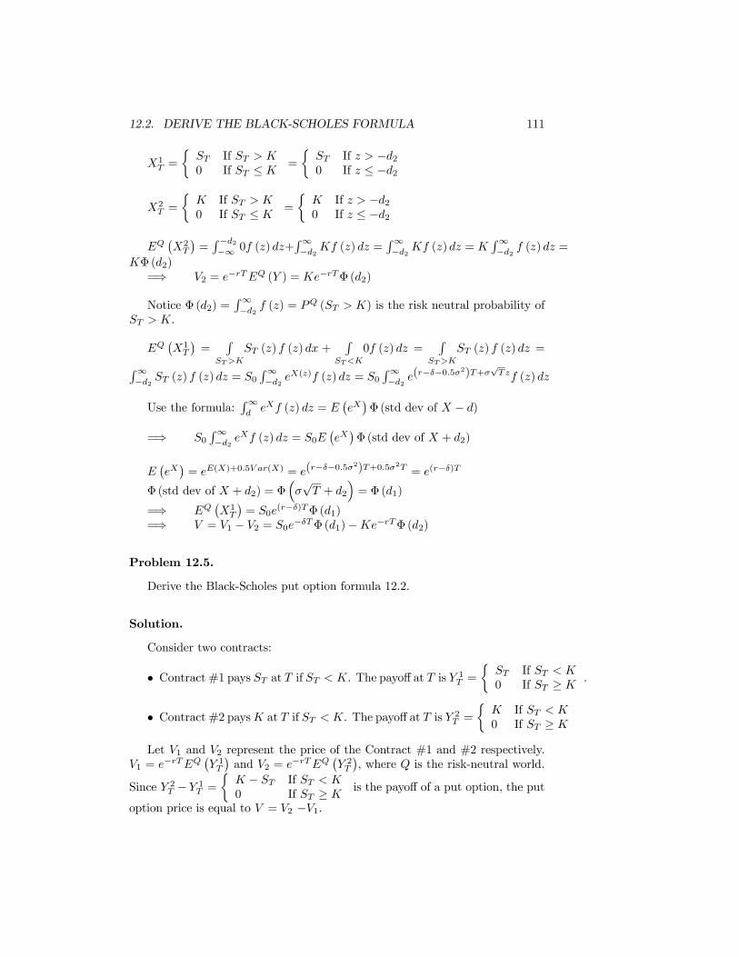
12.2. DERIVE THE BLACK-SCHOLES FORMULA 111
1 =
½ If
0 If ≤ =
½ If −20 If ≤ −2
2 =
½ If
0 If ≤ =
½ If −20 If ≤ −2
¡2
¢=R−2−∞ 0 () +
R∞−2 () =
R∞−2 () =
R∞−2 () =
Φ (2)
=⇒ 2 = − ( ) = −Φ (2)
Notice Φ (2) =R∞−2 () = ( ) is the risk neutral probability of
.
¡1
¢=
R
() () +R
0 () =R
() () =R∞−2 () () = 0
R∞−2
() () = 0R∞−2
(−−052)+√ ()
Use the formula:R∞
() = ¡¢Φ (std dev of − )
=⇒ 0R∞−2
() = 0¡¢Φ (std dev of + 2)
¡¢= ()+05 () = (−−05
2)+052 = (−)
Φ (std dev of + 2) = Φ³√ + 2
´= Φ (1)
=⇒ ¡1
¢= 0
(−)Φ (1)=⇒ = 1 − 2 = 0
−Φ (1)−−Φ (2)
Problem 12.5.
Derive the Black-Scholes put option formula 12.2.
Solution.
Consider two contracts:
• Contract #1 pays at if . The payoff at is 1 =
½ If
0 If ≥ .
• Contract #2 pays at if . The payoff at is 2 =
½ If
0 If ≥
Let 1 and 2 represent the price of the Contract #1 and #2 respectively.
1 = −¡ 1
¢and 2 = −
¡ 2
¢, where is the risk-neutral world.
Since 2 − 1
=
½ − If
0 If ≥ is the payoff of a put option, the put
option price is equal to = 2 −1.

112 CHAPTER 12. BLACK-SCHOLES
Solve () .
→
ln
0− ¡ − − 052¢
√
= −2
Then () is the same as −2. Hence we write 1 and 2
as
follows:
1 =
½ If
0 If ≥ =
½ If −20 If ≤ −2
2 =
½ If
0 If ≥ =
½ If −20 If ≥ −2
¡ 2
¢=R −2−∞ () +
R∞−2 0 () =
R −2−∞ () = Φ (−2)
=⇒ 2 = − ( ) = −Φ (−2)
Φ (−2) =R −2−∞ () = ( ) is the risk neutral probability of
.
¡ 1
¢=R −2−∞ () () +
R∞−2 0 () =
R −2−∞ () () =R−2
−∞ 0 () = 0
R−2−∞ ()
where ∼
£ =
¡ − − 052¢ = 2
¤R −2−∞ () =
¡¢Φ [− (std dev of − (−2))] =
¡¢Φh−³√ + 2
´i=
¡¢Φ (−1)
¡¢= ()+05 () = (−−05
2)+052 = (−)
=⇒ ¡ 1
¢= (−)Φ (−1) 2 = −
£
¡ 1
¢¤= −Φ (−1)
=⇒ = 2 −1 = −Φ (−2)− 0−Φ (−1)
Problem 12.6.
What’s the meaning of Φ (2) and Φ (−2) in the Black-Scholes formula?
Solution.
Φ (2) = ( ) is the risk neutral probability of .
Φ (−2) = ( ) is the risk neutral probability of .
Problem 12.7.
12.2. DERIVE THE BLACK-SCHOLES FORMULA 113
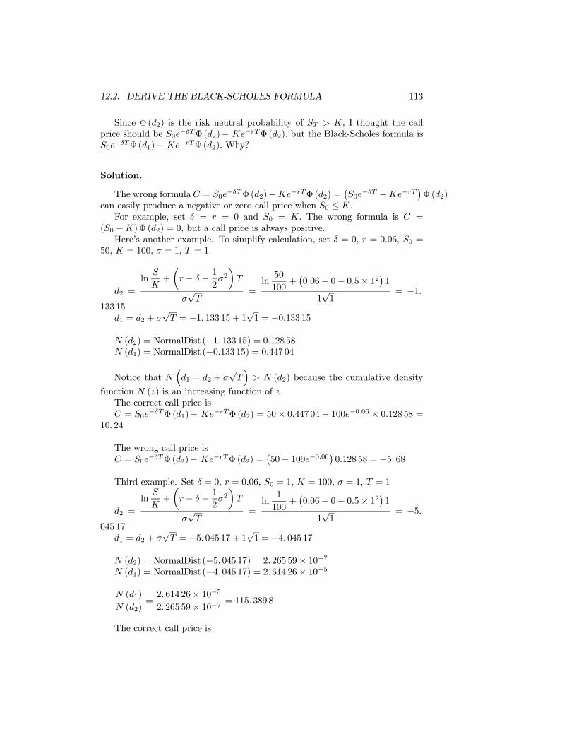
Since Φ (2) is the risk neutral probability of , I thought the call
price should be 0−Φ (2)− −Φ (2), but the Black-Scholes formula is
0−Φ (1)− −Φ (2). Why?
Solution.
The wrong formula = 0−Φ (2)−−Φ (2) =
¡0− −−
¢Φ (2)
can easily produce a negative or zero call price when 0 ≤ .
For example, set = = 0 and 0 = . The wrong formula is =
(0 −)Φ (2) = 0, but a call price is always positive.
Here’s another example. To simplify calculation, set = 0, = 006, 0 =
50, = 100, = 1, = 1.
2 =
ln
+
µ − − 1
22
√
=ln50
100+¡006− 0− 05× 12¢ 1
1√1
= −1133 15
1 = 2 + √ = −1 133 15 + 1√1 = −0133 15
(2) = NormalDist (−1 133 15) = 0128 58 (1) = NormalDist (−0133 15) = 0447 04
Notice that ³1 = 2 +
ë (2) because the cumulative density
function () is an increasing function of .
The correct call price is
= 0−Φ (1)− −Φ (2) = 50× 0447 04− 100−006 × 0128 58 =
10 24
The wrong call price is
= 0−Φ (2)− −Φ (2) =
¡50− 100−006¢ 0128 58 = −5 68
Third example. Set = 0, = 006, 0 = 1, = 100, = 1, = 1
2 =
ln
+
µ − − 1
22
√
=ln
1
100+¡006− 0− 05× 12¢ 1
1√1
= −5045 17
1 = 2 + √ = −5 045 17 + 1√1 = −4 045 17
(2) = NormalDist (−5 045 17) = 2 265 59× 10−7 (1) = NormalDist (−4 045 17) = 2 614 26× 10−5
(1)
(2)=2 614 26× 10−52 265 59× 10−7 = 115 389 8
The correct call price is
114 CHAPTER 12. BLACK-SCHOLES
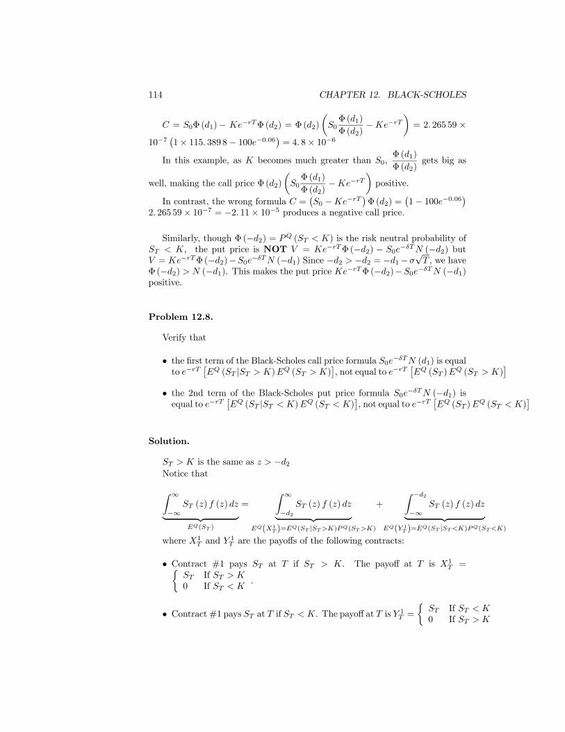
= 0Φ (1)− −Φ (2) = Φ (2)µ0Φ (1)
Φ (2)−−
¶= 2 265 59 ×
10−7¡1× 115 389 8− 100−006¢ = 4 8× 10⁻⁶
In this example, as becomes much greater than 0,Φ (1)
Φ (2)gets big as
well, making the call price Φ (2)
µ0Φ (1)
Φ (2)−−
¶positive.
In contrast, the wrong formula =¡0 −−
¢Φ (2) =
¡1− 100−006¢
2 265 59× 10−7 = −2 11× 10−5 produces a negative call price.
Similarly, though Φ (−2) = ( ) is the risk neutral probability of
, the put price is NOT = −Φ (−2) − 0− (−2) but
= −Φ (−2)−0− (−1) Since −2 −2 = −1−
√ , we have
Φ (−2) (−1). This makes the put price −Φ (−2)−0− (−1)
positive.
Problem 12.8.
Verify that
• the first term of the Black-Scholes call price formula 0− (1) is equalto −
£ ( | ) ( )
¤, not equal to −
£ ( )
( )¤
• the 2nd term of the Black-Scholes put price formula 0− (−1) is
equal to −£ ( | ) ( )
¤, not equal to −
£ ( )
( )¤
Solution.
is the same as −2Notice that
Z ∞−∞
() () | {z }( )
=
Z ∞−2
() () | {z }(1
)=( |)()
+
Z −2−∞
() () | {z }( 1
)=( |)()
where 1 and 1
are the payoffs of the following contracts:
• Contract #1 pays at if . The payoff at is 1 =½
If
0 If .
• Contract #1 pays at if . The payoff at is 1 =
½ If
0 If
12.2. DERIVE THE BLACK-SCHOLES FORMULA 115
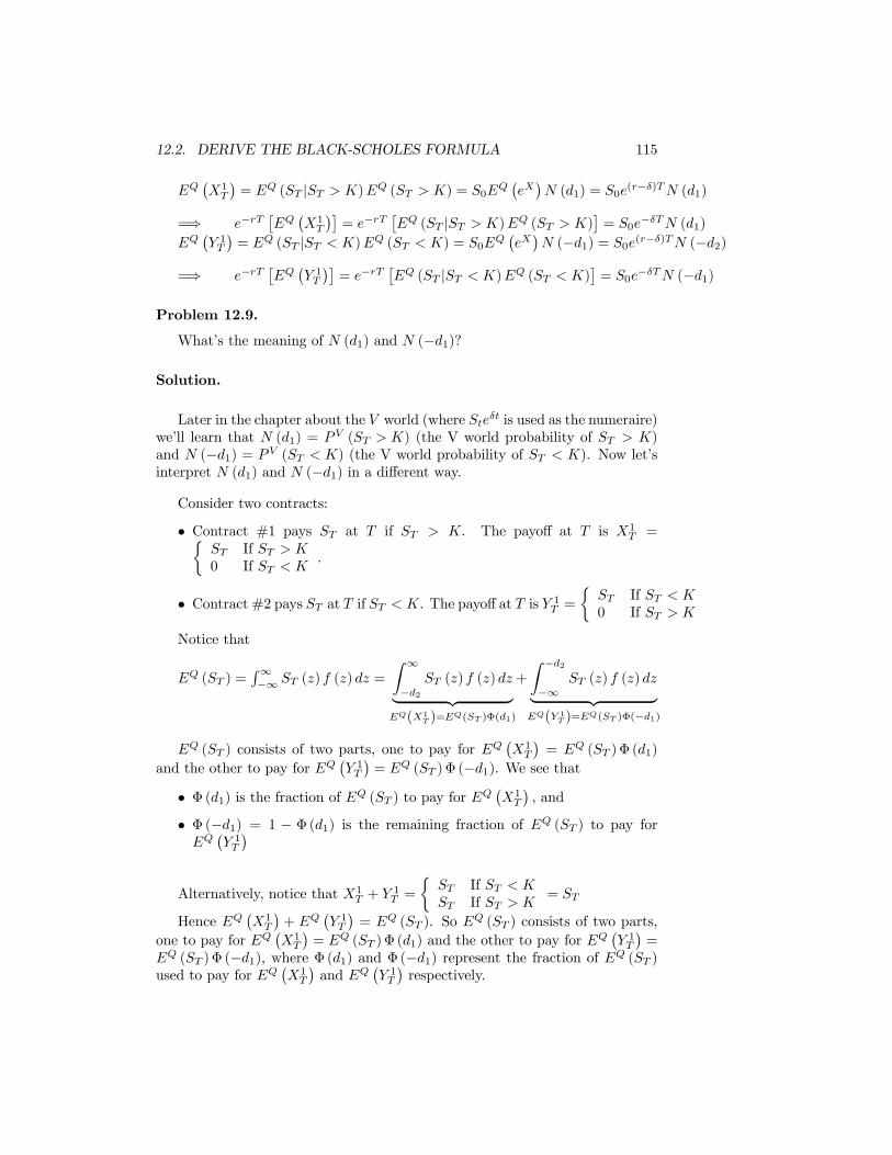
¡1
¢= ( | ) ( ) = 0
¡¢ (1) = 0
(−) (1)
=⇒ −£
¡1
¢¤= −
£ ( | ) ( )
¤= 0
− (1)
¡ 1
¢= ( | ) ( ) = 0
¡¢ (−1) = 0
(−) (−2)
=⇒ −£
¡ 1
¢¤= −
£ ( | ) ( )
¤= 0
− (−1)
Problem 12.9.
What’s the meaning of (1) and (−1)?
Solution.
Later in the chapter about the world (where is used as the numeraire)
we’ll learn that (1) = ( ) (the V world probability of )
and (−1) = ( ) (the V world probability of ). Now let’s
interpret (1) and (−1) in a different way.
Consider two contracts:
• Contract #1 pays at if . The payoff at is 1 =½
If
0 If .
• Contract #2 pays at if . The payoff at is 1 =
½ If
0 If
Notice that
( ) =R∞−∞ () () =
Z ∞−2
() () | {z }(1
)=( )Φ(1)
+
Z −2−∞
() () | {z }( 1
)=( )Φ(−1)
( ) consists of two parts, one to pay for ¡1
¢= ( )Φ (1)
and the other to pay for ¡ 1
¢= ( )Φ (−1). We see that
• Φ (1) is the fraction of ( ) to pay for ¡1
¢ and
• Φ (−1) = 1 − Φ (1) is the remaining fraction of ( ) to pay for
¡ 1
¢Alternatively, notice that 1
+ 1 =
½ If
If =
Hence ¡1
¢+
¡ 1
¢= ( ). So ( ) consists of two parts,
one to pay for ¡1
¢= ( )Φ (1) and the other to pay for
¡ 1
¢=
( )Φ (−1), where Φ (1) and Φ (−1) represent the fraction of ( )
used to pay for ¡1
¢and
¡ 1
¢respectively.

116 CHAPTER 12. BLACK-SCHOLES
Problem 12.10.
A silly option gives its owner the right to receive ln at by paying .
The assumptions under the Black-Scholes formula hold. Calculate the option
price.
Solution.
The option payoff at is =
½ln − If ln
0 If ln ≤ . The option
price at time zero is = − ( ).
= 0 exph¡ − − 052¢ +
√i
Solve ln ln = ln0 +h¡ − − 052¢ +
√i
→ − ln0 −
¡ − − 052¢√
= −∗2
where ∗2 =ln0 − +
¡ − − 052¢√
( ) =R∞−∗2 (ln −) () =
R∞−∗2
hln0 +
¡ − − 052¢ +
√ −
i ()
To calculateR∞−∗2 () , notice that for ∼ (0 1) and () =
1√2
−052
() = 1√2
−052
= −
µ1√2
−052
¶= −
[ ()]
HenceR∞
() =R∞−
[ ()] =
R∞− [ ()] = − () |∞ =
()− (∞) = ()− 0 = ()Z ∞
() = () =1√2
−052
(12.11)
R∞−∗2
hln0 +
¡ − − 052¢ +
√ −
i ()
=R∞−∗2
£ln0 +
¡ − − 052¢ −
¤ () +
√R∞−∗2 ()
=£ln0 +
¡ − − 052¢ −
¤Φ (∗2) +
√ (−∗2)
The option price is
= − ( ) = −£ln0 +
¡ − − 052¢ −
¤×Φ (∗2)+√ (−∗2)Problem 12.11.
12.2. DERIVE THE BLACK-SCHOLES FORMULA 117
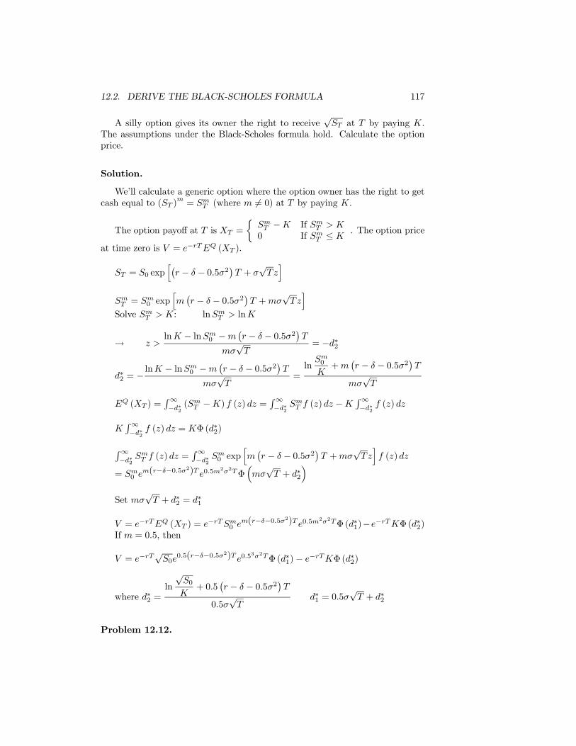
A silly option gives its owner the right to receive√ at by paying .
The assumptions under the Black-Scholes formula hold. Calculate the option
price.
Solution.
We’ll calculate a generic option where the option owner has the right to get
cash equal to ( )= (where 6= 0) at by paying .
The option payoff at is =
½ − If
0 If ≤ . The option price
at time zero is = − ( ).
= 0 exph¡ − − 052¢ +
√i
= 0 exph¡ − − 052¢ +
√i
Solve : ln ln
→ ln − ln0 −
¡ − − 052¢
√
= −∗2
∗2 = −ln − ln0 −
¡ − − 052¢
√
=ln
0
+¡ − − 052¢
√
( ) =R∞−∗2 (
−) () =
R∞−∗2
() −
R∞−∗2 ()
R∞−∗2 () = Φ (∗2)R∞
−∗2 () =
R∞−∗2
0 exp
h¡ − − 052¢ +
√i ()
= 0 (−−052) 05
22Φ³√ + ∗2
´Set
√ + ∗2 = ∗1
= − ( ) = −0 (−−052) 05
22Φ (∗1)−−Φ (∗2)If = 05, then
= −√0
05(−−052) 0532Φ (∗1)− −Φ (∗2)
where ∗2 =ln
√0
+ 05
¡ − − 052¢
05√
∗1 = 05√ + ∗2
Problem 12.12.
118 CHAPTER 12. BLACK-SCHOLES
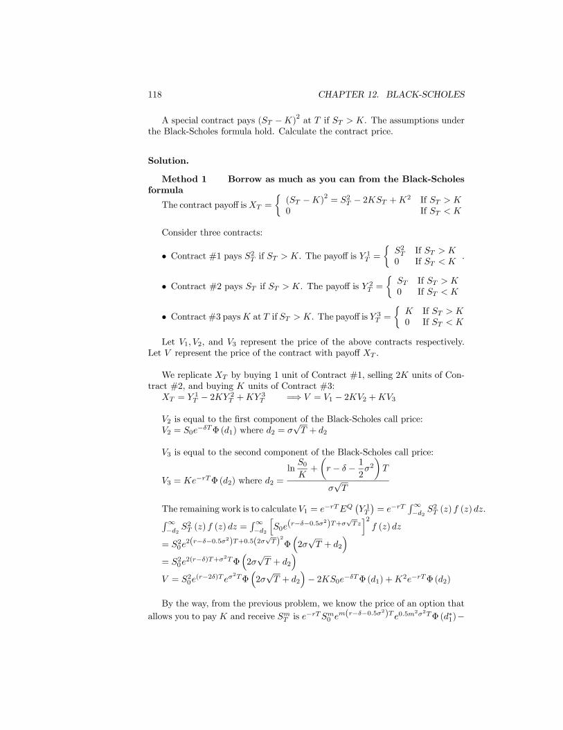
A special contract pays ( −)2at if . The assumptions under
the Black-Scholes formula hold. Calculate the contract price.
Solution.
Method 1 Borrow as much as you can from the Black-Scholes
formula
The contract payoff is =
½( −)
2= 2 − 2 +2 If
0 If
Consider three contracts:
• Contract #1 pays 2 if . The payoff is 1 =
½2 If
0 If .
• Contract #2 pays if . The payoff is 2 =
½ If
0 If
• Contract #3 pays at if . The payoff is 3 =
½ If
0 If
Let 1 2 and 3 represent the price of the above contracts respectively.
Let represent the price of the contract with payoff .
We replicate by buying 1 unit of Contract #1, selling 2 units of Con-
tract #2, and buying units of Contract #3:
= 1 − 2 2
+ 3 =⇒ = 1 − 22 +3
2 is equal to the first component of the Black-Scholes call price:
2 = 0−Φ (1) where 2 =
√ + 2
3 is equal to the second component of the Black-Scholes call price:
3 = −Φ (2) where 2 =ln
0
+
µ − − 1
22
√
The remaining work is to calculate 1 = −¡ 1
¢= −
R∞−2
2 () () .R∞
−2 2 () () =
R∞−2
h0
(−−052)+√i2
()
= 202(−−052)+05(2
√)
2
Φ³2√ + 2
´= 20
2(−)+2Φ³2√ + 2
´ = 20
(−2) 2Φ
³2√ + 2
´− 20
−Φ (1) +2−Φ (2)
By the way, from the previous problem, we know the price of an option that
allows you to pay and receive is −0 (−−052) 05
22Φ (∗1)−
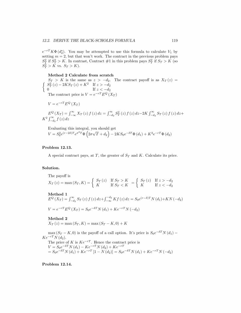
12.2. DERIVE THE BLACK-SCHOLES FORMULA 119
−Φ (∗2). You may be attempted to use this formula to calculate 1 bysetting = 2, but that won’t work. The contract in the previous problem pays
2 if 2 . In contrast, Contract #1 in this problem pays 2 if (so
2 vs. ).
Method 2 Calculate from scratch
is the same as −2. The contract payoff is as () =½2 ()− 2 () +2 If −20 If −2The contract price is = − ( )
= − ( )
( ) =R∞−∞ () () =
R∞−2
2 () () −2
R∞−2 () () +
2R∞−2 ()
Evaluating this integral, you should get
= 20(−2)
2Φ³2√ + 2
´− 20
−Φ (1) +2−Φ (2)
Problem 12.13.
A special contract pays, at , the greater of and . Calculate its price.
Solution.
The payoff is
() = max ( ) =
½ () If
If =
½ () If −2 If −2
Method 1
( ) =R∞−2 () () +
R −2−∞ () = 0
(−) (1)+ (−2)
= − ( ) = 0− (1) +− (−2)
Method 2
() = max ( ) = max ( − 0) +
max ( − 0) is the payoff of a call option. It’s price is 0− (1) −
− (2).The price of is − . Hence the contract price is = 0
− (1)−− (2) +−
= 0− (1) +− [1− (2)] = 0
− (1) +− (−2)
Problem 12.14.

120 CHAPTER 12. BLACK-SCHOLES
A special contract pays | −| at . Calculate its price.
Solution.
The payoff is
() = | −| =½
− If
− If
Method 1
Notice that − If is the payoff of a call option; − If
is the payoff of a put option. Hence the contract price is
= 0− (1)−− (2) +− (−2)− 0
− (−1)= 0
− [ (1)− (−1)]−− [ (2)− (−2)]= 0
− [2 (1)− 1]−− [2 (2)− 1]
Method 2
| −| = 2max ( − 0)− ( −)
2max ( − 0) is twice the payoff of a call option. Its price is 2£0− (1)−− (2)
¤The price of ( −) is 0
− −−
The contract price is
= 2£0− (1)−− (2)
¤− ¡0− −−¢
Problem 12.15.
Derive the gap call price formula DM 14.15.
Solution.
1 is the payment amount; 2 is the payment trigger. The payoff is:
() =
½ ()−1 If 2
0 If 2=
½ ()−1 If −20 If −2
where 2 =
ln0
2
+
µ − − 1
22
√
is calculated by solving:
= 0 exph¡ − − 052¢ +
√i 2
ln2
0−µ − − 1
22
√
= −ln
0
2
+
µ − − 1
22
√
= −2
( ) =R∞−2 [ ()−1] () =
R∞−2 () () −
R∞−2 1 ()
= 0− (1)−1
− (2) where 1 = 2 + √
Related Documents