Deep Learning for Error Prediction In MIMO-OFDM system ...

IN DEGREE PROJECT ELECTRICAL ENGINEERING,SECOND CYCLE, 30 CREDITS

, STOCKHOLM SWEDEN 2018

Deep Learning for Error Prediction In MIMO-OFDM system With Maximum Likelihood Detector

BAOQING SHE

KTH ROYAL INSTITUTE OF TECHNOLOGYSCHOOL OF ELECTRICAL ENGINEERING AND COMPUTER SCIENCE

Abstract

To increase link throughput in multi-input multi-output (MIMO) orthogonal frequency division multiplexing (OFDM) systems, transmission parameters such as code rate and modulation order are required to be set adaptively. Therefore, block error rate (BLER) becomes a crucial measure which illustrates the quality of the link, thus being used in Link Adaptation (LA) to determine the transmission parameters. However, existing methods to predict BLER are only valid for linear detectors, e.g. Minimum Mean Square Error (MMSE) detector [1]. In this thesis, we show that signal-to-interference-plus-noise ratio (SINR) exists in MIMO-OFDM system with MLD (maximum likelihood detection). Then, a machine learning based method with Deep Neural Network (DNN) is proposed to analyze the relation between input features (channel matrix, modulation and coding scheme (MCS), signal-to-noise ratio(SNR)) and labels (CRC). Results shows that the classification of DNN is good. However, there is still deviation when compared output of DNN with the simulated BLER. Index Terms — MIMO-OFDM, CRC, BLER, Detector, SINR, MCS Selection, Link Adaptation,

Deep Learning, Neural Networks

iii

Sammanfattning

För att öka länkhastigheten i MIMO-OFDM system bör överföringsparametrar som kodhastighet och moduleringsordning ändras dynamiskt. Blockfelfrekvensen (BLER) är en viktig komponent i kommunikationssystem som representerar hela länkkedjans status och kan användas i länkanpassning (LA) för att avgöra överföringsparametrarna. Befintliga metoder för att beräkna BLER är endast giltiga för linjära detektorer eg. MMSE. I denna rapport visar vi at SINR existerar i MIMO-OFDM system med MLD. Sedan föreslås en maskininlärningsmetod baserad på djupa neuronnät (DNN) för att analysera förhållandet mellan olika delar av indata (kanal matrix, MCS, SNR) och utdata (CRC). Resultatet visar att DNN klassificerar CRC bra. Utdata från DNN avviker dock vid jämförsele med simulerad BLER.

iv

Acknowledgment

Firstly, I would like to express my special thanks of gratitude to my thesis supervisor Dr. Jinliang Huang, who gave me the opportunity to work at Huawei Sweden AB. I also appreciated the way he showed how to become a good researcher. I would like to thank Gunnar Peters and Stojan Denic for helping me in machine learning implementation. Then, I would like to express my gratitude to Professor Ming Xiao at the department of Information Science and Engineering at Royal Institute of Technology, KTH, who acts as my university thesis examiner. Lastly but not least, I dedicate my thesis to my parents for unconditional love and finance support to help me study at Sweden. I would like to extend my gratitude to my boyfriend Karl Gäfvert for advice on programming and encouragement in life.

v

Contents Abstract ................................................................................................................................................... 2 Sammanfattning ..................................................................................................................................... iii Acknowledgment ................................................................................................................................... iv LIST OF FIGURES ..................................................................................................................................... vi Acronyms ............................................................................................................................................... vii Introduction............................................................................................................................................. 9

1.1. Motivation .................................................................................................................... 9 1.2. Problem Formulation and Method ............................................................................ 10 1.3. Outline of Thesis ........................................................................................................ 11

Background ........................................................................................................................................... 12 2.1 Orthogonal frequency-division multiplexing ..................................................................... 12 2.2 Multiple Antenna Transmission System ............................................................................. 13 2.3 Modulation and Coding Scheme ....................................................................................... 15 2.4 Block Error Rate ................................................................................................................. 17 2.6 Detection Algorithm .......................................................................................................... 17 2.8 Effective SINR ..................................................................................................................... 19 2.5 Link Adaptation .................................................................................................................. 20 2.8 Link to System Mapping ..................................................................................................... 20

Method 22 3.1 MIMO-OFDM Simulation System Configuration ................................................................ 23 3.2 Data Preparation ................................................................................................................ 26

3.2.1 Principle component dimension ....................................................................... 27 3.2.2 Autoencoder ..................................................................................................... 27

3.3 Deep Neural Network Implementation ............................................................................. 29 3.3.1 Block error rate prediction ................................................................................ 29 3.3.2 BLER Evaluation ................................................................................................. 31

Experiment and Discussion ................................................................................................................... 33 4.1 Results................................................................................................................................ 33

4.1.1 Data Preparation ............................................................................................... 33 4.1.2 DNN Performance ............................................................................................. 35 4.1.3 DNN Generalization........................................................................................... 37

4.2 Discussion .......................................................................................................................... 38 Conclusion and Further work ................................................................................................................ 43 BIBLIOGRAPHY....................................................................................................................................... 44

vi

LIST OF FIGURES

Figure 1: Frequency Domain of Sub-Carriers ........................................................................................ 12

Figure 2: OFDM Diagram ....................................................................................................................... 13

Figure 3: MIMO-OFDM Frame ............................................................................................................... 14

Figure 4: Constellation of Different Modulation Scheme ...................................................................... 16

Figure 5: Relation between MCS Index and Code Rate in QPSK, 16QAM, and 64QAM ........................ 17

Figure 6: Projection of Desired Signal after Detector in Signal Space ................................................... 19

Figure 7: Effective SINR mapping using EESM ....................................................................................... 21

Figure 8: Block diagram of the MIMO-OFDM link chain ....................................................................... 23

Figure 9: OD values of EVA channel....................................................................................................... 25

Figure 10: The distribution of BLER over SNR. The dark and light blue line represent MCS16 and MCS15 respectively. The red dot line is the assumed Gaussian PDF of BLER, with 𝜇 = 8, 𝜃 = 14. At the peak of pdf, the BLER of both MCS are around 0.1. .............. 26

Figure 11: Autoencoder Structure ......................................................................................................... 28

Figure 12: Output and Input of DNN ..................................................................................................... 29

Figure 13: sigmoid and tanh activation function ................................................................................... 30

Figure 14: Relation of BLER and effective SINR in Gaussian Channel with Turbo Coding ..................... 32

Figure 15: Explained Variance Ratio of channel .................................................................................... 34

Figure 16: Accuracy of test data with the same Neural Network and different feature dimension reduction ......................................................................................................... 35

Figure 17: Accuracy of test data in Deep Neural Network .................................................................... 36

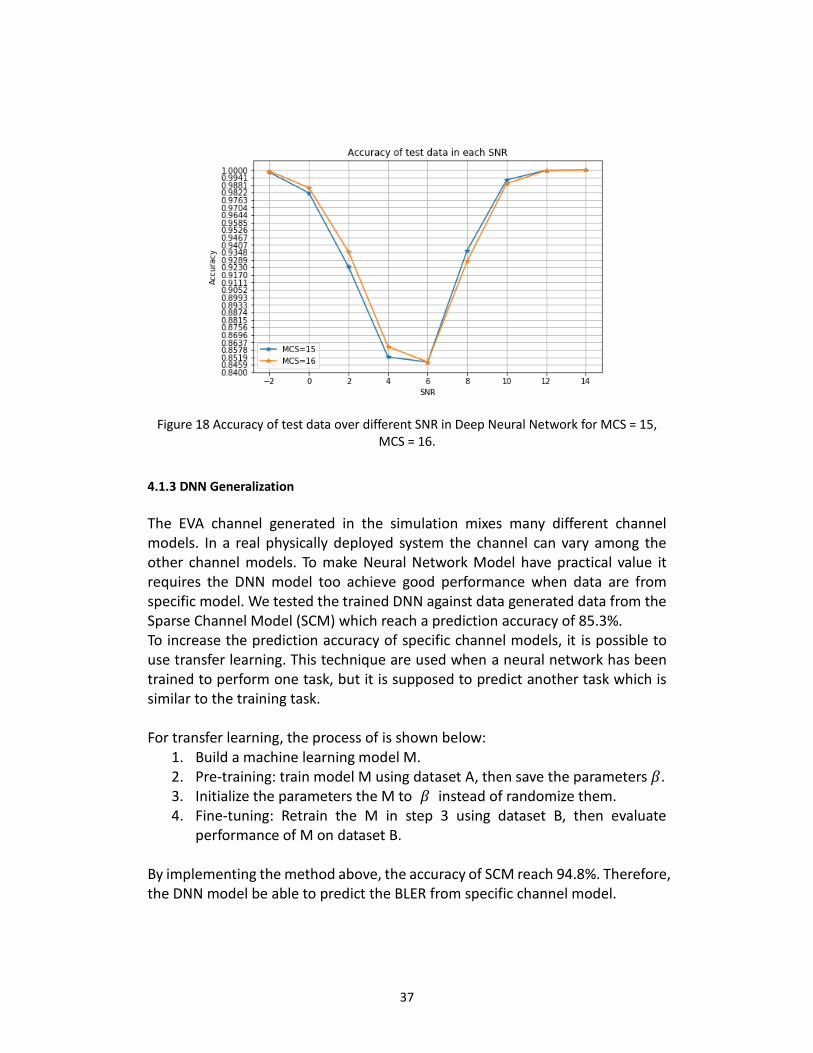
Figure 18 Accuracy of test data over different SNR in Deep Neural Network for MCS = 15, MCS = 16. .................................................................................................................................. 37

Figure 19 the relation between BLER and SNR in non- linear system and ideal linear system when the channel vectors are set to be constant ............................................................. 39

Figure 20 the relation between BLER and effective SINR in non- linear system and ideal linear system ............................................................................................................................... 41

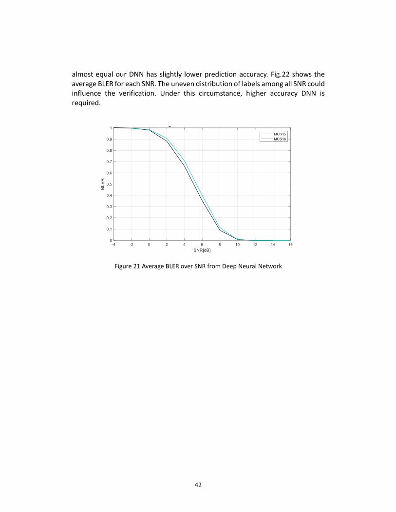
Figure 21 Average BLER over SNR from Deep Neural Network ............................................................. 42

vii

Acronyms MIMO Multiple-input Multiple-output. OFDM Orthogonal Frequency Division Multiplexing. BLER Block Error Rate LA Link Adaptation SNR Signal to Noise Ratio MMSE Minimum Mean Square Error SINR Signal-to-interference-plus-noise ratio MLD Maximum Likelihood Detection MCS Modulation and Code Scheme EESM Exponential Effective SINR Mapping DNN Deep Neural Network 5G Fifth Generation Mobile Communication Systems. UE User Equipment BS Base Station. UL Uplink DMRS Demodulation Reference Signal 3GPP 3rd Generation Partnership Project. FFT Fast Fourier Transform IFFT Inverse Fast Fourier Transform. QAM Quadrature Amplitude Modulation QPSK Quadrature Phase Shift Keying. SCM Spatial Channel Mode PCA Principle Component Analysis EPA Extended Pedestrian model

viii

EVA Extended Vehicular model ETU Extended Typical Urban model RB Resource Block OD Orthogonality Deficient

9

CHAPTER 1 Introduction

1.1. Motivation

The mobile data traffic would increase dramatically in the near future according to [2]. Therefore, fifth generation mobile communication systems (5G) is proposed, where the data rate and throughput are supposed to increase to meet the increasing demand. Several techniques have been proposed to solve the problems caused by high data rate, for example, multiple-input multiple-output (MIMO) system, orthogonal frequency division multiplexing (OFDM), etc. This thesis builds on existing technique in 5G and uses machine learning based method predicting block error rate (BLER) to increase the efficiency and accuracy of uplink. In traditional way of error correcting scheme, receivers evaluate the signal block received by labeling them with binary frame error events (i.e., ACKs/NACKs), where labels equal to 1 means the block is transmitted successfully, otherwise is transmitted with error. Then, the binary frame error events need to be sent to transmitter to decide whether signal block would be transmitted again or not. Using binary frame error events, BLER can be calculated which is utilized to decide the most appropriate modulation and coding scheme (MCS) through specific Link Adaptation (LA) function, which can achieve high throughput. However, obtaining BLER undergoes feedback delay especially when transmitter and receiver are far from each other. Therefore, it would be better if BLER could be predicted at transmitter. It is proved in [1] that BLER can be evaluated in mathematical way given the signal over interference plus noise ratio (SINR) distribution of each sub-carriers and new approximation for Q-function in MMSE detector system. However, according to [3], BLER cannot be evaluated with high accuracy in MIMO-OFDM systems with maximum likelihood detector (MLD), since one of the factor, SINR for each sub-carrier can only be approximated by pulsing the MMSE SINR for each sub-carrier with a gain factor. This gain factor is updated adaptively based on instantaneous channel state and modulation format of interfering streams. Previous work shows method of calculating MLD SINR by adding gain factor is unstable since the equation is too sensitive to the trivial change of

10

environment. In 5G, multi-input multi-output (MIMO) orthogonal frequency division multiplexing (OFDM) link chain is always utilized. Also it is believed that neural network can solve mathematical problems when the formulation is complex. Hence, [4] proposed the possibility of utilizing machine learning in MIMO-OFDM system. Deep Neural Network (DNN) has been implemented in single-input single-output (SISO) system with linear detector to predict block error rate in [5]. Based on previous research, DNN technique is proposed in this thesis to predict BLER in non-linear system using instantaneous channel state and modulation format instead of SINR as the input feature of neural network. The output of DNN is BLER. Here, MLD SINR is a hidden variable of DNN.

1.2. Problem Formulation and Method

In wireless communication systems, Link Adaptation (LA) function is a crucial function, which estimates the most appropriate modulation and coding scheme (MCS) to maximize throughput at given time interval. LA function connects target criterion e.g. a block error rate (BLER) with MCS. However, BLER estimation at transmitter is difficult due to lack of future channel information and link modeling. In this work, we simplify the scenario by assuming perfect channel information at transmitter, but the BLER estimation is still nontrivial because the mapping from a large-size channel matrix to a scalar (BLER) is complicated to model. For OFDM link chain with linear detection, the SINR update of a user equipment (UE) can be calculated. It has been proved that there is specific distribution over instantaneous SINR values and BLER values. Given SINR, BLER can be obtained and then can be used to decide MCS. As showed in [5], DNN (Deep Neural Network) is implemented to obtain the relation between SINR of each sub-carrier with BLER in linear system. Then, the BLER results are used in link adaptation. When the mapping question is extended to non-linear detection, the problem can be further complicated. The SINR for each users are impossible to calculate, which will be illustrated later in Chapter 2. However, it is known that SINR depends on channel estimation and pre-set signal to noise ratio (SNR). Therefore, SINR can be seen as the hidden variable of machine learning model. Then, channel features and SNR are viewed as features of machine learning model, output of model is BLER for UEs. The objectives of this thesis project are:

11

Use DNN model to predict BLER for each UE, in which channel estimation and SNR are provided as input features, and binary frame error events (i.e., ACKs/NACKs) are used as labels.

As labels are classified into 0 and 1, this is a classification problem where cross entropy is used as loss function. Compare the predicted ACK/NACK with simulated results and get prediction accuracy.

The output of the DNN is actually a probability which indicates the

possibilities for 0 (NACK) and 1 (ACK), which can be compared with the simulated BLER to find out whether the classification result is good enough for a regression problem.

1.3. Outline of Thesis

This report is organized as following. In Chapter 2, the basic knowledge about MIMO-OFDM system as well as some related properties of communication system are briefly presented, which is necessary to understand the whole report. Chapter 3 shows the method used for data preparation and machine learning algorithm implementation, following by Chapter 4 which provides the results of experiments. Furthermore, there is also discussion about the experiment results in Chapter 4. Chapter 5 summarizes the report and gives future work for this topic.

12

CHAPTER 2 Background

2.1 Orthogonal frequency-division multiplexing

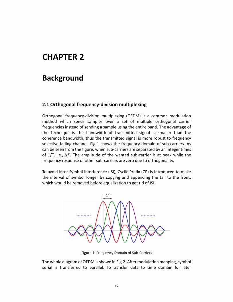
Orthogonal frequency-division multiplexing (OFDM) is a common modulation method which sends samples over a set of multiple orthogonal carrier frequencies instead of sending a sample using the entire band. The advantage of the technique is the bandwidth of transmitted signal is smaller than the coherence bandwidth, thus the transmitted signal is more robust to frequency selective fading channel. Fig 1 shows the frequency domain of sub-carriers. As can be seen from the figure, when sub-carriers are separated by an integer times of 1/T, i.e., ∆𝑓 . The amplitude of the wanted sub-carrier is at peak while the frequency response of other sub-carriers are zero due to orthogonality. To avoid Inter Symbol Interference (ISI), Cyclic Prefix (CP) is introduced to make the interval of symbol longer by copying and appending the tail to the front, which would be removed before equalization to get rid of ISI.

Figure 1: Frequency Domain of Sub-Carriers

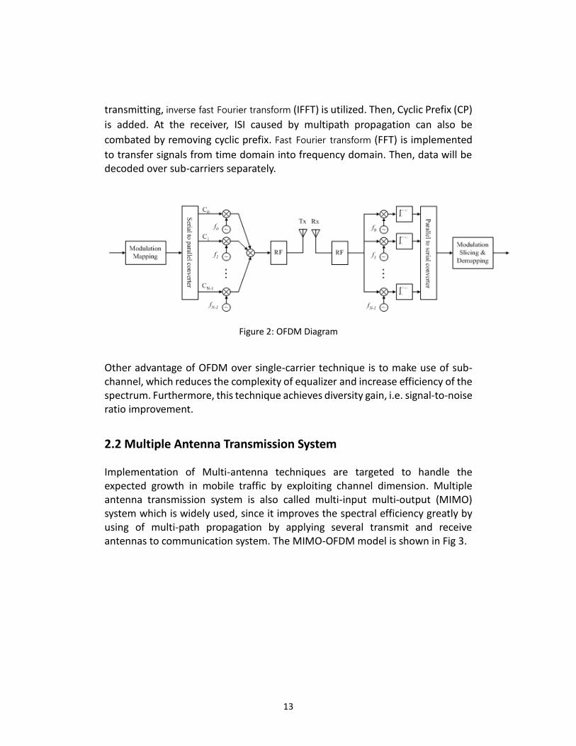
The whole diagram of OFDM is shown in Fig.2. After modulation mapping, symbol serial is transferred to parallel. To transfer data to time domain for later

13

transmitting, inverse fast Fourier transform (IFFT) is utilized. Then, Cyclic Prefix (CP)

is added. At the receiver, ISI caused by multipath propagation can also be

combated by removing cyclic prefix. Fast Fourier transform (FFT) is implemented

to transfer signals from time domain into frequency domain. Then, data will be decoded over sub-carriers separately.

Figure 2: OFDM Diagram

Other advantage of OFDM over single-carrier technique is to make use of sub-channel, which reduces the complexity of equalizer and increase efficiency of the spectrum. Furthermore, this technique achieves diversity gain, i.e. signal-to-noise ratio improvement.

2.2 Multiple Antenna Transmission System

Implementation of Multi-antenna techniques are targeted to handle the expected growth in mobile traffic by exploiting channel dimension. Multiple antenna transmission system is also called multi-input multi-output (MIMO) system which is widely used, since it improves the spectral efficiency greatly by using of multi-path propagation by applying several transmit and receive antennas to communication system. The MIMO-OFDM model is shown in Fig 3.

14

Figure 3: MIMO-OFDM Frame

Assume a MIMO system with 𝑁𝑡 transmit antennas and 𝑁𝑟 receive antennas. We can express received signal 𝑦 as:

𝑦 = 𝐻𝑥 + 𝑤 (1)

Where, 𝑥 is the transmitted signal through different antennas, hence 𝑥 =[𝑥1, 𝑥2, … , 𝑥𝑁𝑡

] , 𝑦 = [𝑦1, 𝑦2, … , 𝑦𝑁𝑟 ] is the received signal, 𝐻 is a complex

channel matrix with dimension [𝑁𝑡, 𝑁𝑟], where ℎ𝑖𝑗 is transfer functions from

the j-th transmit antenna to the i-th receive antenna. 𝑤 is complex Gaussian noise vector. Except for MIMO scheme, communication system has three other types according to the number of antennas used in transceivers.

SISO, Single-input single-output, where 𝑁𝑟= 1, 𝑁𝑡 = 1. SIMO, single-input multiple-output, where 𝑁𝑟= n, 𝑁𝑡 = 1. MISO, multiple-input single-output, where 𝑁𝑟= 1, 𝑁𝑡 = n.

In MIMO system, based on different transmit scheme, there are three main techniques used, i.e., space diversity, spatial multiplexing and beamforming. Space diversity technique, which helps eliminate channel fading effect, is to obtain many copies of the data and then transmit the copies through different transmit antennas. Hence, the same data is transmitted at different transmit antennas at same time. Different multiple antennas experience different propagation path and being affected differently, thus achieve eliminating channel fading effect. For spatial multiplexing MIMO system, which increases the data

15

rate, uses the technique to split data into multiple sub-streams, which means different antennas transmit different data stream. Another MIMO technique is Beamforming [5]. At the receiver, original data would be recovered either by selecting the best received signal or by combining the information antennas received. The key of using MIMO technology is to effectively avoid interference between antennas to distinguish among multiple parallel data streams. However, if the channel is frequency selective, it becomes difficult to recover data because the inter-antenna interference and the inter-symbol interference are mixed together. Since channels within each OFDM sub-carriers (with a bandwidth of only 15 kHz) can be considered as flat fading channels. Combining MIMO with OFDM can obtain high data while guarantee the accuracy of data transmit.

2.3 Modulation and Coding Scheme

Modulation is the technique changing one or more properties of the carrier signal. When transmitting signal, information bits need to be modulated before being sent, while at receiver, signal need to be demodulated. The aim of modulation is to increase transmitting efficiency by transferring bits into symbol. Then symbols are used to adjust property of carrier signal, i.e., frequency, amplitude or phase. Quadrature amplitude modulation (QAM) is a method adjusts the amplitude of carrier signal. There many types of modulation depending on numbers of bits in one symbol, e.g., QPSK (4QAM), 16QAM, and 64QAM. The constellation of them are shown in Fig 4. For QPSK, one black spot has 2 bits, i.e., 00, 01, 11 or 11. Similarly, 16QAM and 64QAM utilize 4 bits and 6 bits to represent a symbol respectively. Low-order modulation guarantee the quality of signal while the data rate is relatively low. High-order modulation has high data rate while the quality of signal cannot be guaranteed. Therefore, only when channel is good condition, the high-order modulation is suggested.

16

Figure 4: Constellation of Different Modulation Scheme

By implementing channel coding, error detection and correction can be done at receiver, since some redundant bits are added to spread the information carried on several bits to more bits. This technique guarantee the accuracy of transmitting by adding redundancy at the cost of transmitting more bits than are needed. The code rate is decided by transport block sizes, resource block sizes.

𝑐𝑜𝑑𝑒 𝑟𝑎𝑡𝑒

=𝑡𝑎𝑛𝑠𝑝𝑜𝑟𝑡 𝑏𝑙𝑜𝑐𝑘 𝑠𝑖𝑧𝑒

𝑟𝑒𝑠𝑜𝑢𝑟𝑐𝑒 𝑏𝑙𝑜𝑐𝑘 𝑠𝑖𝑧𝑒

(2)

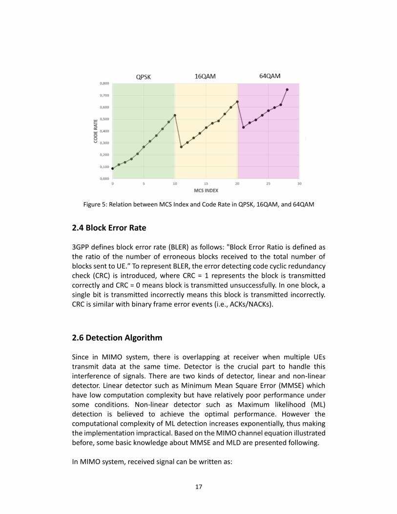
Modulation and Coding Scheme together decide throughput and data rate of a communication system. MCS index is introduced to represent possible Modulation and Coding Scheme, which is composed by modulation order, transport block sizes, resource block numbers. It is shown in Fig 5, MCS index is linearly related to the code rate.

17

Figure 5: Relation between MCS Index and Code Rate in QPSK, 16QAM, and 64QAM

2.4 Block Error Rate

3GPP defines block error rate (BLER) as follows: "Block Error Ratio is defined as the ratio of the number of erroneous blocks received to the total number of blocks sent to UE.” To represent BLER, the error detecting code cyclic redundancy check (CRC) is introduced, where CRC = 1 represents the block is transmitted correctly and CRC = 0 means block is transmitted unsuccessfully. In one block, a single bit is transmitted incorrectly means this block is transmitted incorrectly. CRC is similar with binary frame error events (i.e., ACKs/NACKs).

2.6 Detection Algorithm

Since in MIMO system, there is overlapping at receiver when multiple UEs transmit data at the same time. Detector is the crucial part to handle this interference of signals. There are two kinds of detector, linear and non-linear detector. Linear detector such as Minimum Mean Square Error (MMSE) which have low computation complexity but have relatively poor performance under some conditions. Non-linear detector such as Maximum likelihood (ML) detection is believed to achieve the optimal performance. However the computational complexity of ML detection increases exponentially, thus making the implementation impractical. Based on the MIMO channel equation illustrated before, some basic knowledge about MMSE and MLD are presented following. In MIMO system, received signal can be written as:

18

𝑦 = 𝐻𝑥 + 𝑤 = ∑ ℎ𝑖𝑠𝑖

𝑛

𝑖=1

+ 𝑤 (3)

ℎ𝑖 represents 𝑖𝑡ℎ column of complex channel matrix H with dimension [𝑁𝑡, 𝑁𝑟]. 𝑠𝑖 is the transmitted signal with normalized power from the 𝑖𝑡ℎ transmitter. MMSE detector: Linear detection algorithm for MIMO detection correlates the received signals linearly with a matrix G to obtain corresponding decision information. For MMSE detector, G is the matrix to minimize the mean square error between the detected signal and the desired signal:

𝐺 = arg min𝑊

𝐸[|𝑥 − 𝐺𝑦|2] (4)

To obtain decision on transmitted signal s1 for the first user among other UEs, the interference can be viewed as noise too. Hence, (3) can be rewritten as:

𝑦 = ℎ1𝑠1 + 𝑛 (5)

Where, 𝑛 is colored noise. Then a whiten filter is required to the colored noises become white again. This filter is basically the inverse proportional to the power of interference and noise. For k-th UE, the filter is given as:

𝐺 = 𝑁 + 𝑃 ∑ ℎ𝑖ℎ𝑖∗

𝑖≠𝑘

(6)

𝐺−12𝑦 = 𝐺−

12𝐻𝑥 + 𝐺−

12𝑛

(7)

Where, N is the power of white noise and P is the uniform power of all transmitted signals. Then, apply matched filter to the signals that have gone through whiten filter to project the filtered signal against the direction GH:

(𝐺−12𝐻)

𝐻

𝐺−12 = 𝐻𝐻𝐺−1𝐻𝑠

+ 𝐻𝐻𝐺−1𝑛

(8)

Therefore, MMSE detector is:

19

𝐺 =𝐻𝐻

𝐻𝐻𝐻 + 𝑁𝐼𝑁𝑟

(9)

ML detector: ML detection utilize an optimal algorithm for detection, since it searches through the whole space of transmit signal i.e., all possible transmitted vectors to find optimal solution. Hence, the complexity of ML increase exponentially as the length of one signal vector. The mathematical equation of ML is shown:

𝑥𝑀�̂� = arg 𝑚𝑖𝑛 min𝑥∈𝑆

𝑁𝑡|𝑦 − 𝐻𝑥|2 (10)

𝑆𝑁𝑡 is the space of all the possible combination for a transmit symbol. ML

detection has to search all the 𝑆𝑁𝑡 candidate symbol combinations for the

optimal solutions.

2.8 Effective SINR

The SINR is the effective signal to noise ratio after filtering transmitted signal with linear detectors. Fig 6 shows the geometric way of illustrating how detector works. Detector project the received signal to the projection vector. However, there is deviation between the real desired signal 𝑠1 and the projected signal. Therefore, effective SINR is introduced to present this deviation.

Figure 6: Projection of Desired Signal after Detector in Signal Space

For MMSE detector, the effective SINR can be written as:

20

𝑆𝐼𝑁𝑅𝑒𝑓𝑓𝑐𝑡𝑖𝑣𝑒 ,𝑛

=𝑆𝑁𝑅

[(𝐻𝐻𝐻 + 𝑁𝐼𝑁𝑟)

−1]𝑛𝑛

(11)

Where n denotes the nth output stream, and [. ]𝑛𝑛denotes the nth diagonal element in the matrix. To be concrete, in this thesis, we assume the SINR in this thesis is effective SINR we mention here.

2.5 Link Adaptation

The purpose of Link Adaptation [4] is to optimize the system capacity and coverage under a certain transmission power. The transmitter should match the data transmission rate and the received signal quality. The BS selects the MCS according to the link adaptation algorithm. The algorithm can be designed by using BLER among others. The overall process is:

When the base station receives the Physical Uplink Shared Channel (PUSCH) from the UE, the base station measures effective SINR of the PUSCH according to the demodulation reference signal (DMRS).

BS physical layer reports the effective SINR to higher layers. According to the link simulation, the effective SINR is used to select MCS. The link adaptation module passes the MCS to the resource allocation

module to calculate other parameters, e.g., TBS (transport).

2.8 Link to System Mapping

Approaches of link to system mapping [6] such as Exponential Effective SINR Mapping (EESM) and Mutual Information based Effective SINR Mapping (MI-ESM) are wildly used in wireless communication system, where EESM requires all the sub-carriers in OFDM/multi-carrier system level using same modulation and coding scheme (MCS), while it is not necessary for (MI-ESM). In OFDM system, each sub-carrier has sub-SINR. For one instantaneous channel state, we obtain SINR vector {𝛾𝑘} = (𝛾1, 𝛾2 … 𝛾𝑛) at moment k for a set of sub-carriers (the number of sub-carrier is n). Every sub-SINR can be mapped to corresponding BLER using the relation between 𝑆𝐼𝑁𝑅 and BLER under AWGN channel. However, different sub-carriers are dependent, the BLER for the whole

21

system is not simply add the BLER of all sub-carriers together. Therefore, we need a scale parameter 𝛽 to scale sub-carriers and get an equivalent overall 𝑆𝐼𝑁𝑅𝑒𝑓𝑓

for OFDM system, then use this 𝑆𝐼𝑁𝑅𝑒𝑓𝑓 to do mapping to obtain BLER, which

is correct for whole system. It was proposed in [7] and [8] to use function map vector SINR 𝛾𝑘 to 𝑆𝐼𝑁𝑅𝑒𝑓𝑓,

which is a scalar value. To guarantee the algorithm correctly, the following function need to be achieved.

𝐵𝐿𝐸𝑅𝐴𝑊𝐺𝑁(𝛾𝑒𝑓𝑓) = 𝐵𝐿𝐸𝑅𝐴𝑊𝐺𝑁({𝛾𝑘})

Where, 𝐵𝐿𝐸𝑅𝐴𝑊𝐺𝑁() is a function to map SINR to BLER under AWGN channel.

𝐵𝐿𝐸𝑅𝐴𝑊𝐺𝑁({𝛾𝑘}) is the actual block error rate for given channel state. The equation above should be satisfied for every moment k, not only works for average BLER for several moment.

This 𝑆𝐼𝑁𝑅𝑒𝑓𝑓 will be interrupted as effective SINR in this thesis. Since BLER is a

function of the Modulation and Coding Scheme (MCS), the number of allocated Resource Blocks (RBs), the SINR, each MCS corresponds to a single BLER curve when fix RBs, which is shown in the right figure of Fig.7. Therefore, EESM methods are used to calculate the effective SINR and then maps it to BLER. The BLER curve is chosen depending on the MCS index.

Figure 7: Effective SINR mapping using EESM

22

CHAPTER 3 Method

In previous chapters, the problems are briefly introduced. In this chapter, problem is illustrated in more detail as well as the experiment configuration. Then, method used to solve the problem is proposed. As the link adaptation is a crucial part to guarantee throughput of telecommunication system, which has been introduced in the background part. Hence, when increasing the speed of data traffic, quick decision should be made to choose proper Modulation and Coding scheme (MCS) to achieve maximum throughput. It is known that Block Error Rate decide the MCS through the link adaptation function. Therefore, it is believe that if the distribution of the BLER over SINR is known, then BLER can be used in link adaptation function to decide the order of modulation and the coding rate. Machine learning method has been proposed in linear detection system [5] to predict BLER, by using SINR for each sub-carriers as input features. Then, the link adaptation can be done more efficiently and accurately. However, there are a lot of obstacles to implement machine learning method into the non-linear system, since the SINR for each sub-carriers in linear OFDM system can be calculated using mathematical method, but not in non-linear OFDM system. As shown in the background part, although MLD is believed to achieve optimal results, it has complex structure, thus impossible to obtain the mathematical equation to calculate SINR. Since deep neural network is justified to represent the complicated non-linear relation between input and output and it is known that SINR depends on channel estimation and SNR, machine learning method is proposed to find the value of BLER when given channel estimation and SNR as input. The complicated mathematical equation can be represented by the network. Here, SINR viewed as a hidden variable in the machine learning model. The exact value of SINR still cannot be obtained, but it is known one possible combination of channel vectors and SNR value is a SINR and feed this combination as the input of DNN, then the corresponding error events are obtained from the output of DNN. Then, simulated BLER is utilized to compare with the output of DNN to verify the

23

regression problem. Justification details will be shown in section 3.3. The structure of chapter is order as following: Section 3.1 describes MIMO-OFDM simulation platform configuration in this thesis, e.g. RBs, channel model, UE deployment etc., and following by section 3.2 giving the structure of raw data from the simulator as well as method of data pre-process for machine learning model training. Section 3.3 presents deep neural network implementation and results evaluation.

3.1 MIMO-OFDM Simulation System Configuration

In the MIMO-OFDM simulation system. There are four UE, and each UE is equipped with one antenna in the cell. The simulation only test uplink scenario, where signals are transmitted from users to BS that is equipped with four receive antennas. Hence, the whole system is a MU-MIMO model (Multi User Multi Input Multi Output), which is shown in Fig 8.

Here, one transmitted block 𝑏 = (𝑏1, 𝑏2, … , 𝑏𝑛) carry n bits information from one UE. These bits will go through coding module, where, extra bits will be add into block to enable the receiver calibrate error later. Then, coded information

H BLER

Info from UEs

16QAM Modulation

MLD Detection

De-rate match Turbo Decoding

OFD Multiplexing

Channel Estimation

Info Sink

Error event:𝑒𝑘: 𝑏 = 𝑏

OFD De-Multiplexing

PHY- Channel

Rate match Turbo Coding

MCS Selection

Transmitter

Receiver

Figure 8: Block diagram of the MIMO-OFDM link chain

24

will enter modulation module to transfer bits into symbols. Assume 𝑀 is the modulation order, one out of 2𝑀 complex-valued constellation symbols will be represented each M-tuple of bits. For 16QAM, the order M = 4, which means 4 bits are utilized to represent one symbol, and there are 16 possible complex-valued constellation symbols to choose from. Finally, a length- 𝑁𝑠𝑢𝑏 IFFT operation is applied on each group of 𝑁𝑠𝑢𝑏 modulated symbols to generate the frame OFDM symbols and mapped onto physical resources. 𝑁𝑠𝑢𝑏 represents number of subcarriers, which depend on Resource Block (RB). One Resource Block (RB) contains 12 subcarriers. In the simulation, RB is set to 6, i.e. there are 72 subcarriers in one OFDM symbol.

The frame OFDM symbols are transmitted over Gaussian channel. We assume that the channel vector remains constant for the frame OFDM symbols. Therefore, only one out of 14 OFDM symbols is selected to extract the channels of all subcarriers. The power of both noise and signals are normalized in this system. When doing channel estimation at receiver, the SNR value is included in the estimated channel vector, i.e., the amplitude of estimated channel is scaled by SNR. Hence, SNR wouldn’t be feed as an individual feature for the neural network when training in this thesis.

At receiver, reconstructed bit sequence is represented as �̂� = (𝑏1, 𝑏2, … 𝑏𝑛). We define the block error event at the receiver as:

𝑒 = {1, 𝑏 ≠ 𝑏

0, 𝑏 = 𝑏

Here, the block error event is different from CRC mentioned before. The reason will be illustrated in 3.3.1. In wireless systems a transmitted signal results in several signals at receiver with relatively low power due to the signal reflection between transceivers. Delay spread describes the time differences between the first arrival multipath component and the last arrival multipath component. Delay spread is correlated with environment between transceivers and a larger delay spread indicates a highly dispersive channel. 3GPP defines three multipath fading channel models: Extended Pedestrian model (EPA), Extended Vehicular model (EVA), and Extended Typical Urban model (ETU); which are representatives of low, medium, and high delay spread environments respectively. In our simulation, the EVA channel model is used. Fig.15 shows the Orthogonality Deficiency (OD) of our EVA channel in one subcarrier. OD is a metric to show the orthogonality of the channel vector of one UE to the others. OD equal

25

to zero means the vectors are orthogonal. The OD values vary which shows that the EVA channel used has good generalization.

Figure 9: OD values of EVA channel

Table 1 shows parameters of MIMO-OFDM simulation. Our system is a 4x4 MIMO system where each UE have 72 subcarriers. The dimension of the channel is calculated as72 × 4 × 4 = 1152. Each channel is represented by a complex value. However, due to complex values increasing the difficulty in training ANN the real part and imaginary part of the channel are viewed as different features, i.e., the total dimension of channel features are doubled to 2304. As mentioned before, as the dimension of features increase, neural network requires large number of training data to obtain good results. Hence, low dimensional features with good correlation are always preferred if possible. In next section, data preparation to reduce feature dimension will be provided.

Table 1: Parameters of MIMO-OFDM Simulation

Simulation Parameters Value

Cell Number UEs Number

BS Receive antennas Channel Model

RB Number Transmit Subcarriers Number of each UE

Modulation MCS order

1 4 4

EVA 6

72 16QAM [15,16]

26

3.2 Data Preparation

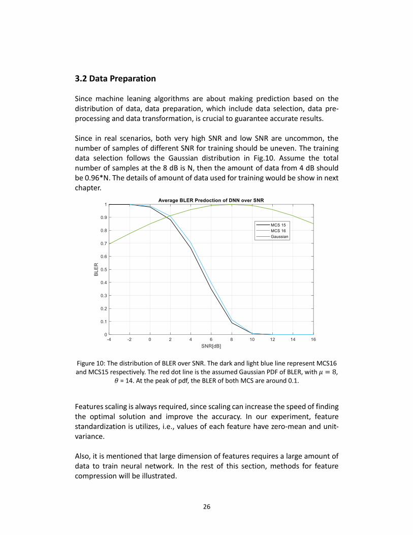
Since machine leaning algorithms are about making prediction based on the distribution of data, data preparation, which include data selection, data pre-processing and data transformation, is crucial to guarantee accurate results. Since in real scenarios, both very high SNR and low SNR are uncommon, the number of samples of different SNR for training should be uneven. The training data selection follows the Gaussian distribution in Fig.10. Assume the total number of samples at the 8 dB is N, then the amount of data from 4 dB should be 0.96*N. The details of amount of data used for training would be show in next chapter.

Figure 10: The distribution of BLER over SNR. The dark and light blue line represent MCS16 and MCS15 respectively. The red dot line is the assumed Gaussian PDF of BLER, with 𝜇 = 8,

𝜃 = 14. At the peak of pdf, the BLER of both MCS are around 0.1.

Features scaling is always required, since scaling can increase the speed of finding the optimal solution and improve the accuracy. In our experiment, feature standardization is utilizes, i.e., values of each feature have zero-mean and unit-variance. Also, it is mentioned that large dimension of features requires a large amount of data to train neural network. In the rest of this section, methods for feature compression will be illustrated.

27

The dimension of input channel feature of neural network is 2304, since only real value can be feed into neural network, the real part and imagination part of complex channel should be separated, thus double the original dimension of channel feature. If the input feature of a neural network is high dimension, a large amount of data is required for training the network to obtain high accuracy. Hence, data pre-processing is required to reduce the dimension of data. Two different methods to decrease channel dimension are implemented in this thesis, i.e., PCA (Principle Component Analysis) and Autoencoder. In this section, both algorithm will be presented in the rest of this section.

3.2.1 Principle component dimension

Principle component dimension (PCA) is a commonly used data analysis method. PCA transforms the original data into a set of linearly independent representations of each dimension through linear transformation, which can be used to extract the main feature components of the data. It is often used to reduce the dimensions of high-dimensional data. PCA uses the eigenvector of the covariance matrix as the projection direction. The projection direction is chosen by maximizing the variance of the data after the projection. To reduce the original data to k dimensions, the eigenvalues are sorted by descending order, then the eigenvector corresponding to the eigenvalue whose value rank largest k are used as the projection direction. In chapter 4, implementation details and discussion about PCA will be given.

3.2.2 Autoencoder

Autoencoder algorithm aims to compress dimension of data while minimize the information loss. Different from PCA, Autoencoder take the non-linear relation between data into consideration. Autoencoder is an unsupervised learning algorithm that uses a back-propagation algorithm [10] to make the target value equal to the input value. As Fig 11 shows:

28

Figure 11: Autoencoder Structure

X is the input data, z is the encoded X, X’ is the output. There are encoder and decoder in the Autoencoder structure. Encoder part is used when to obtain encoded data from the model. Decoder part is only used when training Autoencoder model. Autoencoder tries to reduce data dimension by learning a function. The function somehow represents the difference of X and X’, which means if X = X’, it achieves optimal encoder results. That is, the Autoencoder tries to approximate an identity function shown below, making the output close to the input:

𝑄𝑤,𝑏(𝑋) = 𝑋 Where, w and b are the parameters of the network, and 𝑄𝑤,𝑏(. ) is the identity function. By implementing Autoencoder, compressed representations of input data, i.e. z, can be obtained. Since Autoencoder is basically a neural network, it requires training. For training phase, it is similar to train a Neural Network. A loss function is required to optimize the parameters of network. In this thesis, the mean absolute error loss function is used, since the aim of the Autoencoder is to make the input and output equal, which guarantee the encoded variable z contains the information to reconstruct X. The mathematical expression is shown below. Then, Backpropagation algorithm is used to optimize the parameters of network.

𝑀𝐸𝐴 =∑ |𝑋 − 𝑋′|𝑛

𝑖=0

𝑛

29

After training process finish, test data would be feed to model to obtain the encoded data from the encoder part. For a good Autoencdoer model, the encoded data has lower dimension as well as contains correlation of the input data i.e., all the necessary information for reconstructing it to original data. In chapter 4, implementation details of Autoencoder and performance comparison with PCA will be provided.

3.3 Deep Neural Network Implementation

3.3.1 Block error rate prediction

Since link adaptation need parameters BLER to update MCS selection, it is crucial to obtain BLER after detector. However, for non-linear detector it is hard to compute the SINR due to the complex mathematical relation involving many parameters. Furthermore, traditional way of computing BLER by utilizing EESM approach [6] cannot guarantee optimality of the corresponding BLER prediction, since it approximates channel vectors into scalar, shown in [5]. Therefore, it is proposed to use Deep Neural Network (DNN) to solve this problem. Although neural network is believed excellent when solving non-linear mathematical functions, the process inside network is still hard to be understood totally which prevent the application of neural network in many field. The DNN in this thesis is supposed to predict BLER by using uncompressed channel vector among other features. The abstract idea of the DNN is shown in Fig.12.

Figure 12: Output and Input of DNN

BLER_1, BLER_2, BLER_3 and BLER_4 are the BLER for four users in one cell respectively. In this neural network, the labels are the error events of four users when they transmit one signal block to BS the same time. The MCS scheme and RB numbers are the same for four users. In previous work, the sorted per-subcarrier SINR vector are used as the input to the network [5] in SISO system. However, in MIMO system, there is still no solution to SINR calculation. It is known that SINR depends on estimated channel matrix at receiver and SNR. Hence, deep neural network is feed with uncompressed channel matrix as well as SNR here. It

30

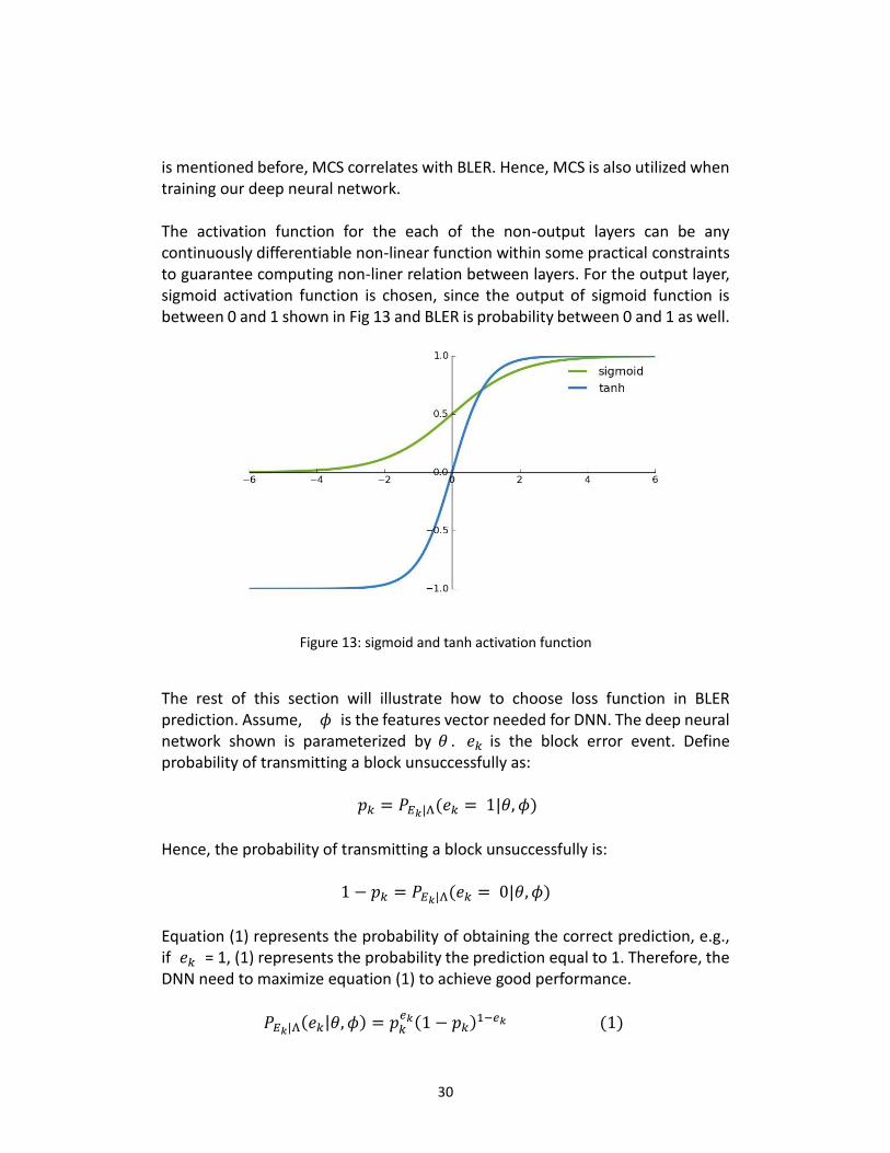
is mentioned before, MCS correlates with BLER. Hence, MCS is also utilized when training our deep neural network. The activation function for the each of the non-output layers can be any continuously differentiable non-linear function within some practical constraints to guarantee computing non-liner relation between layers. For the output layer, sigmoid activation function is chosen, since the output of sigmoid function is between 0 and 1 shown in Fig 13 and BLER is probability between 0 and 1 as well.

Figure 13: sigmoid and tanh activation function

The rest of this section will illustrate how to choose loss function in BLER prediction. Assume, 𝜙 is the features vector needed for DNN. The deep neural network shown is parameterized by 𝜃 . 𝑒𝑘 is the block error event. Define probability of transmitting a block unsuccessfully as:

𝑝𝑘 = 𝑃𝐸𝑘|Λ(𝑒𝑘 = 1|𝜃, 𝜙)

Hence, the probability of transmitting a block unsuccessfully is:

1 − 𝑝𝑘 = 𝑃𝐸𝑘|Λ(𝑒𝑘 = 0|𝜃, 𝜙)

Equation (1) represents the probability of obtaining the correct prediction, e.g., if 𝑒𝑘 = 1, (1) represents the probability the prediction equal to 1. Therefore, the DNN need to maximize equation (1) to achieve good performance.

𝑃𝐸𝑘|Λ(𝑒𝑘|𝜃, 𝜙) = 𝑝𝑘𝑒𝑘(1 − 𝑝𝑘)1−𝑒𝑘 (1)

31

Then, make some transformation of (1), (2) is obtained:

𝐿(𝜃) = − 1

𝐾∑ ln 𝑃𝐸𝑘|Λ(𝑒𝑘|𝜃, 𝜙)

𝐾

𝑖=1

= − 1

𝐾∑ 𝑒𝑘𝑙𝑛𝑝𝑘 + (1 − 𝑒𝑘)ln (1 − 𝑝𝑘)

𝐾

𝑖=1

(2)

Where, K represents the number of samples. As can be seen, equation (2) is cross entropy loss function. Good performance of neural network can be achieved by minimizing the cross entropy loss function above.

3.3.2 BLER Evaluation

To verify the BLER predicted using DNN, the relation of BLER and effective SINR in Gaussian Channel with Turbo Coding is used, which is shown in Fig.14. As can be seen from the figure, different MCS has different curve to represent the relation between BLER and effective SINR, i.e., the BLER of different MCS varies given the same effective SINR. In this section, how to use this property to verify our results will be illustrated. Since we know that the SINR of system is decided by both channel matrix and SNR, channel matrix and SNR fixed means the effective SINR unchanged. As mentioned before, estimated channel including SNR value in this system, in the rest of this thesis, channel features are referred to channel matrix plus SNR feature. The step of verifying the BLER prediction of DNN is shown below:

Choose data with the same channel features and different MCS feature, i.e., 𝐷1, 𝐷2 are dataset with MCS=15, MCS=16 respectively.

Obtain the BLER of 𝐷1 and 𝐷2 by utilizing DNN, obtain the estimated BLER vector 𝜶 and 𝜷.

Given 𝜶, use the theoretical BLER curve with MCS =15 shown in Fig.14 to find the corresponding effective SINR 𝜸.

Plot the distribution of 𝜷 over 𝜸, obtain the estimated curve. Compare the estimated curve from last step with the BLER curve

shown in Fig.14 In the next chapter, the detail will be provided.

32

Figure 14: Relation of BLER and effective SINR in Gaussian Channel with Turbo Coding

33

CHAPTER 4 Experiment and Discussion

In chapter 3, the problem as well as the method to solve and verify the solution to the problem are provided. In this chapter the simulation results as well as discussion will be presented. This chapter is divided into two sections. Section 4.1 shows simulation results, following by section 4.2, where verification is performed by using the BLER predictions from the trained DNN model and comparing them with true BLER values obtained from a classical model.

4.1 Results

4.1.1 Data Preparation

In this sub section a feature reduction strategy is chosen. PCA linear dimension reduction method and Autoencoder non-linear feature compression are implemented and compared. a) PCA The basic principles of PCA are provided in section 3.3.1. In this section, the implementation of PCA in our simulation system will be presented. Since it is required to keep the principal components with large variance to guarantee the most necessary information is saved after reduction, the variance i.e. eigenvalues of all the possible eigenvectors have to be computed to decide how many dimension are to be kept. Here, the explained variance ratio is introduced:

𝜆𝑗

∑ 𝜆𝑗𝑑𝑗=1

𝜆𝑗 is the eigenvalue of j-th eigenvector. 𝑑 is total feature dimension. The explained variance ratio of all principals are shown in Fig.16. As can be seen from the figure it is reasonable to keep the number of principal components below or equal to 100 since the useful information the remaining principal components can represent is limited. In our simulation 𝑛 = {50, 70, 100} are being tested. However, the increment of accuracy of DNN from 𝑛 = 70 to 𝑛 = 100 is trivial.

34

Therefore it is believed that n = 100 is enough to represent all the necessary information. The dimension of channel feature is reduced to 100 after implementing PCA in this experiment.

Figure 15: Explained Variance Ratio of channel

b) Autoencoder

As mentioned before, PCA is used for linear feature compression. Since it is possible that the correlation between channels are non-linear a large amount of useful information can be neglected when using a linear dimension reduction method. Hence a non-linear feature transform is also implemented to capture the non-linear relation between features. However, an Autoencoder is basically a neural network, which means a large amount of extra training data are required to train the networks separately. To compare the results of Autoencoder with PCA, dimension of channel will also be reduced to 100 after implementing Autoencoder.

35

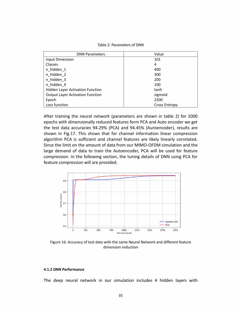
Table 2: Parameters of DNN

DNN Parameters Value

Input Dimension Classes n_hidden_1 n_hidden_2 n_hidden_3 n_hidden_4 Hidden Layer Activation Function Output Layer Activation Function Epoch Loss function

101 4 400 300 200 100 tanh sigmoid 2200 Cross Entropy

After training the neural network (parameters are shown in table 2) for 1000 epochs with dimensionally reduced features form PCA and Auto encoder we get the test data accuracies 94.29% (PCA) and 94.45% (Auroencoder), results are shown in Fig.17. This shows that for channel information linear compression algorithm PCA is sufficient and channel features are likely linearly correlated. Since the limit on the amount of data from our MIMO-OFDM simulation and the large demand of data to train the Autoencoder, PCA will be used for feature compression. In the following section, the tuning details of DNN using PCA for feature compression will are provided.

Figure 16: Accuracy of test data with the same Neural Network and different feature dimension reduction

4.1.2 DNN Performance

The deep neural network in our simulation includes 4 hidden layers with

36

dimensions [400; 300; 200; 100] respectively with 𝑡𝑎𝑛ℎ activation function. In the output layer the sigmoid activation function is used. The training results of Deep Neural Network is shown in Fig.17. In the figure, the accuracy of training data reach its peak of 94.84% around 2200 epochs. The maximum accuracy of test data is 97.12%.

Figure 17: Accuracy of test data in Deep Neural Network

However, when test the test data accuracy over SNR, the performance of each SNR varies. As can be seen in Fig.18, the accuracy can reach 100% at SNR = 14dB, while the accuracy at SNR = 6dB is only 84.81%.

37

Figure 18 Accuracy of test data over different SNR in Deep Neural Network for MCS = 15, MCS = 16.

4.1.3 DNN Generalization

The EVA channel generated in the simulation mixes many different channel models. In a real physically deployed system the channel can vary among the other channel models. To make Neural Network Model have practical value it requires the DNN model too achieve good performance when data are from specific model. We tested the trained DNN against data generated data from the Sparse Channel Model (SCM) which reach a prediction accuracy of 85.3%. To increase the prediction accuracy of specific channel models, it is possible to use transfer learning. This technique are used when a neural network has been trained to perform one task, but it is supposed to predict another task which is similar to the training task. For transfer learning, the process of is shown below:

1. Build a machine learning model M. 2. Pre-training: train model M using dataset A, then save the parameters 𝛽. 3. Initialize the parameters the M to 𝛽 instead of randomize them. 4. Fine-tuning: Retrain the M in step 3 using dataset B, then evaluate

performance of M on dataset B.

By implementing the method above, the accuracy of SCM reach 94.8%. Therefore, the DNN model be able to predict the BLER from specific channel model.

38

Accuracy of SCM data without Pre-training 85.3%

Accuracy of SCM data with Pre-training 94.8%

By implementing Pre-training, relatively smaller amount of data and less training epoch are required to achieve good performance.

4.2 Discussion

In this section, link to system mapping, which is mentioned in section 2.8, will be used to verify the results of BLER prediction. Following is a general function to project effective SINR to BLER in Gaussian channel.

𝐵𝐿𝐸𝑅 = 𝐹(𝛾𝑒𝑓𝑓)

It is known that 𝛾𝑒𝑓𝑓 is the identified effective SINR when the channel vector

and SNR are fixed, then corresponding BLER can be obtained by using the equation above. A. Verify effective SINR and BLER in MIMO simulation To justify the existence of SINR in MIMO systems using MLD, the BLER over effective SINR in ideal Gaussian channel is use as reference. Since it is believed that SINR depends on channel estimation and SNR, i.e. the noise of channel, the BLER would vary with SNR when the channel vector is kept unchanged. Hence, there is a certain distribution between BLER and SNR when the channel is constant in the MIMO simulator. The comparison is shown in Fig. 21. The blue and black line show the relation between BLER and SNR of UE#2 in MIMO simulator, with MCS = 16 and MCS = 15 respectively. The dash lines show the corresponding distribution of BLER in Gaussian channel. The slopes of BLER curves in the MLD system are approximately the same as those in the Gaussian channel, which means changing SNR i.e., changing amplitude of channel, the BLER curve follows the same trend as that in Gaussian channel. Hence, the relation between BLER over channel and SNR is not random, but follows a similar trend as BLER distribution over SINR in ideal Gaussian channel. As can be seen in the figure, there are deviation between the distribution in MIMO-OFDM simulator and that in Gaussian channel. This happens since the MLD used in this MIMO-OFDM system does not achieve the optimal results.

39

When fixing the SNR value on x axis, e.g. 𝛾𝑚𝑐𝑠15 = 𝛾𝑚𝑐𝑠16 = 6.6 𝑑𝐵 . The corresponding BLER values of two MCS in the MIMO system can be obtained by projecting over the solid lines in the figure. Then the obtained BLER values are used to find the corresponding SNR value �̅�𝑚𝑐𝑠15, �̅�𝑚𝑐𝑠16 in Gaussian channel by using the dash line in the figure. Since the channel is constant, the SNR value difference between 𝛾, �̅� is the SINR difference. Since the𝛾𝑚𝑐𝑠15 = 𝛾𝑚𝑐𝑠16 and the trend of solid and dash line are supposed to be the same, it is expected that �̅�𝑚𝑐𝑠15 = �̅�𝑚𝑐𝑠16. However, the difference varies in the range [0.03, 0.07] dB. It is mentioned before, MLD used in system does not use fully exhaustive search. Also TTI is only 1000. Consider all above, the deviation [0.03, 0.07] dB is within experimental error range. Therefore, we assume SINR exists in the MIMO-OFDM MLD system.

Figure 19 the relation between BLER and SNR in non- linear system and ideal linear system when the channel vectors are set to be constant

B. Verify estimated BLER from DNN In previous section, it have been proved that SINR exist in the system utilizing MLD. In this section, evaluation of the BLER predicted by deep neural network will be provided.

It is assumed that if the BLER prediction from DNN for both MCS follows the

40

similar trend as that in Gaussian channel, the BLER values predicted by DNN are justified. Since the specific value of SINR in the MIMO MLD system cannot be obtained. To plot the distribution of BLER over SINR, the method in section 3.3.2 is used. It is assumed that the relation between BLER and SINR follows the theoretical distribution curve in Gaussian channel when MCS = 15 (shown as the blue line in Fig. 22). Since the test samples have the same channel the features should have the same effective SINR. After obtaining the BLER for MCS = 15, the corresponding SINR can be found by using the theoretical BLER distribution curve in Gaussian channel. Hence, the corresponding SINR of MCS = 16 dataset has the same channel features as MCS = 15 can be obtained. Then, using these post-SINR results and corresponding BLER predicted by DNN for MCS = 16, the green line in Fig.22 can be obtained, which is the distribution of BLER predicted by Deep Neural Network. The red line in Fig.22 shows the theoretical BLER curve with MCS = 16 in Gaussian channel. However, there is a deviation between the green line and the red line, i.e. given the effective SINR, the BLER predicted by DNN is lower than the ideal BLER in theory by 0.2 dB. After several experiments, we found that as the prediction accuracy of DNN increases, this difference becomes smaller. There are many reasons to explain this difference between real experimental results and ideal one.

41

Figure 20 the relation between BLER and effective SINR in non- linear system and ideal linear system

As mentioned before, MLD does not achieve optimal results which can cause the data used to train Deep Neural Network to have a bias. Also, the data generated from Matlab simulation has its own limitations. For example, the influence between antennas are neglected in the simulator. The solution to this problem is utilizing the real data from BS to eliminate the bias existing in training data. Also, in this thesis the channel vectors are assumed to remain constant for the frame OFDM symbols. Therefore, only one out of 14 OFDM symbols is selected to extract the channels of all subcarriers. However, the channel vectors are not absolutely unchanged with an OFDM frame. Hence, neglecting this information can cause the mismatch of practical and theoretical results. Another possible reasons is that channel vectors in the training data for each MCS index is not repeatable. This can be solved by training the DNN using more data with the same channel vectors and changing SNR value. Except the reasons mentioned above, the accuracy of this DNN can also lead to the slight offsets in the results. Although the accuracy of prediction (test data) can reach 94.84% average over all the SNR, the prediction accuracy varies in each SNR depend on the distribution of error events as shown in Fig.18. For relatively high SNR, most of the data tend to be transmitted correctly. Hence only several or no labels are 1 among a larger portion of the samples, for which DNN can predict with high accuracy. For SNR where the number of labels with 1 and 0 are

42

almost equal our DNN has slightly lower prediction accuracy. Fig.22 shows the average BLER for each SNR. The uneven distribution of labels among all SNR could influence the verification. Under this circumstance, higher accuracy DNN is required.

Figure 21 Average BLER over SNR from Deep Neural Network

43

CHAPTER 5 Conclusion and Further work

In this thesis, the distribution of BLER and SINR in MIMO system with ML detector are studied. The simulation results show that SINR not only exist in linear communication system but also in non-linear system. There are 0.03 dB bias when comparing the distribution of the BLER over SINR in this MIMO-OFDM simulation with ideal relation in Gaussian channel. This offset is probably due to that MLD used in system is not exhaustive, i.e., not all the possibility are considered when doing detection, among other reasons. Then, a deep learning approach is proposed for BLER prediction in MIMO system with ML detector, since the high complexity of the relation between BLER and SINR. A 4-layers Deep Neural Network is designed, which utilize channel vectors, the power of noise and MCS as input features. Although the overall performance of error prediction (ACK/NACK) based on DNN is good (96%), for specific range of SNR the accuracy become relatively lower (84% in the worst case), which influence the justification results. Furthermore, the predicted error probability from DNN does not generally reflect the real BLER, i.e., the results from classification cannot be directly used as a result for regression problem (to predict BLER). To sum up, the DNN designed to predict BLER in this thesis has decent performance. There are several possible way to help improve the performance of DNN method predicting BLER by decreasing the bias of results. Future direction is to improve the performance of DNN to predict more accurate error probability. Firstly, we can improve the training data collection by labeling the training data with real BLER. Secondly, the training data can be obtained from more different channel models for better generalization of the DNN. Since the process inside network is still hard to be understood totally, instead of feed all the features in a neural network, it is required to design based on the known relations between features.

44

BIBLIOGRAPHY

[1] N. Kim, Y. Lee and H. Park, "Performance Analysis of MIMO System with Linear MMSE Receiver," in IEEE Transactions on Wireless Communications, vol. 7, no. 11, pp. 4474-4478, November 2008. [2]https://www.ericsson.com/en/mobility-report/future-mobile-data-usage-and-traffic-growth [3] T. Abe and G. Bauch, "Effective SINR Computation for Maximum Likelihood Detector in MIMO Spatial Multiplexing Systems," GLOBECOM 2009 - 2009 IEEE Global Telecommunications Conference, Honolulu, HI, 2009, pp. 1-5. [4] R. C. Daniels, C. M. Caramanis and R. W. Heath, "Adaptation in Convolutionally Coded MIMO-OFDM Wireless Systems Through Supervised Learning and SNR Ordering," in IEEE Transactions on Vehicular Technology, vol. 59, no. 1, pp. 114-126, Jan. 2010 [5] Vidit Saxena, Joakim Jaldén, Hugo Tullberg, Mats Bengtsson, "DEEP LEARNING FOR FRAME ERROR PROBABILITY PREDICTION IN BICM-OFDM SYSTEMS", Oct. 30, 2017 [6] David Tse and Pramod Viswanath Cambridge University Press, 2005,'Fundamentals of Wireless Communication' [7] P. Bertrand, J. Jiang and A. Ekpenyong, "Link Adaptation Control in LTE Uplink," 2012 IEEE Vehicular Technology Conference (VTC Fall), Quebec City, QC, 2012, pp. 1-5. [8] E. Tuomaala and Haiming Wang, "Effective SINR approach of link to system mapping in OFDM/multi-carrier mobile network," 2005 2nd Asia Pacific Conference on Mobile Technology, Applications and Systems, Guangzhou, 2005, pp. 5 pp.-5. [9] Pekka Lavila, "Dynamic Mapping Between Link and System Level Simulators". Master's Thesis, Univ. Of Helsinki, 2004. [10] P. J. Werbos, "Backpropagation through time: what it does and how to do it," in Proceedings of the IEEE, vol. 78, no. 10, pp. 1550-1560, Oct. 1990. doi: 10.1109/5.58337

45

TRITA TRITA-EECS-EX-2018:485

ISSN 1653-5146

www.kth.se