Deep Learning for Automatic Speech Recognition – Part III Xiaodong Cui IBM T. J. Watson Research Center Yorktown Heights, NY 10598 Fall, 2018

Welcome message from author
This document is posted to help you gain knowledge. Please leave a comment to let me know what you think about it! Share it to your friends and learn new things together.
Transcript

Deep Learning for Automatic SpeechRecognition – Part III
Xiaodong Cui
IBM T. J. Watson Research CenterYorktown Heights, NY 10598
Fall, 2018

Deep Learning for Computer Vision, Speech, and Language
Outline
• End-to-end acoustic modeling
I Connectionist Temporal Classification (CTC)
I Encoder-decoder attention models
• Other techniques in acoustic modeling
I Data augmentation
I Speaker adaptation (transfer learning)
I Multilingual acoustic modeling
EECS 6894, Columbia University 2/50

Deep Learning for Computer Vision, Speech, and Language
Two Streams of DNN Acoustic Models
• Hybrid DNNs (discussed last lecture)I Commonly referred to as DNN-HMM or CD-DNN-HMMI Use GMM-HMM alignments as labelsI Use dictionary and language model for decoding.
• End-to-end (E2E) DNNsI Directly deal with sequence-to-sequence mapping problem with
unequal sequence lengthsI Do not need alignments, dictionary and language model in
principle.I Two E2E architectures:
I Connectionist Temporal Classification (CTC)I Encoder-Decoder Attention models
EECS 6894, Columbia University 3/50

Deep Learning for Computer Vision, Speech, and Language
Connectionist Temporal Classification (CTC)
Mathematical Formulation:
• Input: Observation sequence X = {x1, x2, · · · , xT}
• Label: Target sequence Z = {z1, z2, · · · , zM}
• Unequal lengths: M < T
• Model: A neural network with a softmax output layer
Z = Nλ(X)
• Loss function: Maximum likelihood
λ∗ = argmaxλ
logPλ(Z|X)
EECS 6894, Columbia University 4/50

Deep Learning for Computer Vision, Speech, and Language
CTC Paths• Allowing blanks and repeated labels (L′ = L ∪ {�})
B(a�aabb��) = B(�aa��abb) = ab
• Same length as the input sequence• Many-to-one mapping• Likelihood of the path π (conditional independency)
P (π|X) =T∏t=1
ytπt, ∀π ∈ L′T
where πt = k and ytk is the output of the softmax layer, outputunit k at time t.• Likelihood of the label sequence
P (Z|X) =∑
π∈B−1(Z)
p(π|X)
EECS 6894, Columbia University 5/50
Deep Learning for Computer Vision, Speech, and Language
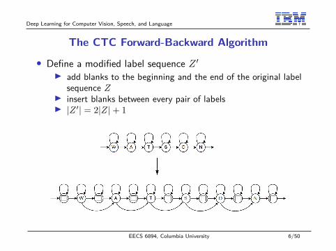
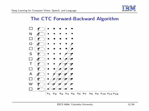
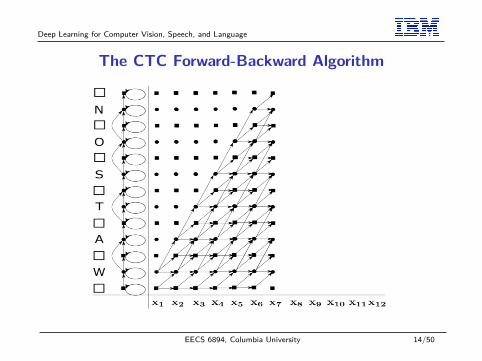
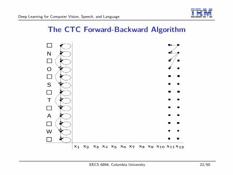
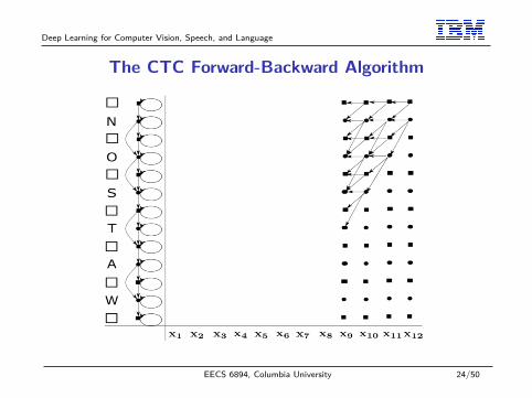
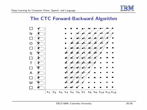
The CTC Forward-Backward Algorithm
• Define a modified label sequence Z ′I add blanks to the beginning and the end of the original label
sequence ZI insert blanks between every pair of labelsI |Z ′| = 2|Z|+ 1
EECS 6894, Columbia University 6/50

Deep Learning for Computer Vision, Speech, and Language
The CTC Forward-Backward Algorithm
EECS 6894, Columbia University 7/50

Deep Learning for Computer Vision, Speech, and Language
The CTC Forward-Backward Algorithm
EECS 6894, Columbia University 8/50

Deep Learning for Computer Vision, Speech, and Language
The CTC Forward-Backward Algorithm
EECS 6894, Columbia University 9/50

Deep Learning for Computer Vision, Speech, and Language
The CTC Forward-Backward Algorithm
EECS 6894, Columbia University 10/50

Deep Learning for Computer Vision, Speech, and Language
The CTC Forward-Backward Algorithm
EECS 6894, Columbia University 11/50
Deep Learning for Computer Vision, Speech, and Language
The CTC Forward-Backward Algorithm
EECS 6894, Columbia University 12/50

Deep Learning for Computer Vision, Speech, and Language
The CTC Forward-Backward Algorithm
EECS 6894, Columbia University 13/50
Deep Learning for Computer Vision, Speech, and Language
The CTC Forward-Backward Algorithm
EECS 6894, Columbia University 14/50

Deep Learning for Computer Vision, Speech, and Language
The CTC Forward-Backward Algorithm
EECS 6894, Columbia University 15/50

Deep Learning for Computer Vision, Speech, and Language
The CTC Forward-Backward Algorithm
EECS 6894, Columbia University 16/50

Deep Learning for Computer Vision, Speech, and Language
The CTC Forward-Backward Algorithm
EECS 6894, Columbia University 17/50

Deep Learning for Computer Vision, Speech, and Language
The CTC Forward-Backward Algorithm
EECS 6894, Columbia University 18/50

Deep Learning for Computer Vision, Speech, and Language
The CTC Forward-Backward Algorithm
EECS 6894, Columbia University 19/50

Deep Learning for Computer Vision, Speech, and Language
The CTC Forward-Backward Algorithm
EECS 6894, Columbia University 20/50

Deep Learning for Computer Vision, Speech, and Language
The CTC Forward-Backward Algorithm
EECS 6894, Columbia University 21/50
Deep Learning for Computer Vision, Speech, and Language
The CTC Forward-Backward Algorithm
EECS 6894, Columbia University 22/50

Deep Learning for Computer Vision, Speech, and Language
The CTC Forward-Backward Algorithm
EECS 6894, Columbia University 23/50
Deep Learning for Computer Vision, Speech, and Language
The CTC Forward-Backward Algorithm
EECS 6894, Columbia University 24/50

Deep Learning for Computer Vision, Speech, and Language
The CTC Forward-Backward Algorithm
EECS 6894, Columbia University 25/50

Deep Learning for Computer Vision, Speech, and Language
The CTC Forward-Backward Algorithm
EECS 6894, Columbia University 26/50

Deep Learning for Computer Vision, Speech, and Language
The CTC Forward-Backward Algorithm
EECS 6894, Columbia University 27/50

Deep Learning for Computer Vision, Speech, and Language
The CTC Forward-Backward Algorithm
EECS 6894, Columbia University 28/50
Deep Learning for Computer Vision, Speech, and Language
The CTC Forward-Backward Algorithm
EECS 6894, Columbia University 29/50

Deep Learning for Computer Vision, Speech, and Language
The CTC Forward-Backward Algorithm
EECS 6894, Columbia University 30/50

Deep Learning for Computer Vision, Speech, and Language
The CTC Forward-Backward Algorithm
EECS 6894, Columbia University 31/50

Deep Learning for Computer Vision, Speech, and Language
The CTC Forward-Backward Algorithm
EECS 6894, Columbia University 32/50
Deep Learning for Computer Vision, Speech, and Language
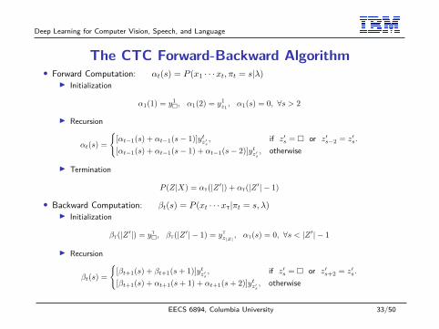
The CTC Forward-Backward Algorithm• Forward Computation: αt(s) = P (x1 · · ·xt, πt = s|λ)I Initialization
α1(1) = y1�, α1(2) = y1
z1, α1(s) = 0, ∀s > 2
I Recursion
αt(s) ={
[αt−1(s) + αt−1(s− 1)]ytz′s, if z′s = � or z′s−2 = z′s.
[αt−1(s) + αt−1(s− 1) + αt−1(s− 2)]ytz′s, otherwise
I Termination
P (Z|X) = αT(|Z ′|) + αT(|Z ′| − 1)
• Backward Computation: βt(s) = P (xt · · ·xT|πt = s, λ)I Initialization
βT(|Z ′|) = yT�, βT(|Z ′| − 1) = yT
z|Z|, αT(s) = 0, ∀s < |Z ′| − 1
I Recursion
βt(s) ={
[βt+1(s) + βt+1(s+ 1)]ytz′s, if z′s = � or z′s+2 = z′s.
[βt+1(s) + αt+1(s+ 1) + αt+1(s+ 2)]ytz′s, otherwise
EECS 6894, Columbia University 33/50
Deep Learning for Computer Vision, Speech, and Language
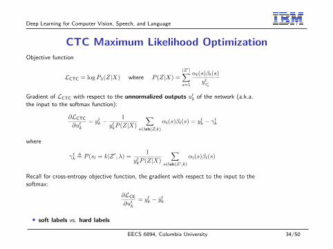
CTC Maximum Likelihood OptimizationObjective function
LCTC = logPλ(Z|X) where P (Z|X) =|Z′|∑s=1
αt(s)βt(s)ytz′s
Gradient of LCTC with respect to the unnormalized outputs utk of the network (a.k.a.the input to the softmax function):
∂LCTC∂utk
= ytk −1
ytkP (Z|X)∑
s∈lab(Z,k)αt(s)βt(s) = ytk − γtk
where
γtk , P (st = k|Z ′, λ) = 1ytkP (Z|X)
∑s∈lab(Z′,k)
αt(s)βt(s)
Recall for cross-entropy objective function, the gradient with respect to the input to thesoftmax:
∂LCE∂utk
= ytk − ytk
• soft labels vs. hard labels
EECS 6894, Columbia University 34/50

Deep Learning for Computer Vision, Speech, and Language
CTC DecodingAlex Graves mentioned two decoding strategy in his seminal CTC paper• Best path decoding
h(X) ≈ B(π∗)
where
π∗ = argmaxπ∈Nt
p(π|X)
simply concatenate the most active outputs at each time-step, notguaranteed to find the most probable labeling• Prefix search decoding with beam searchI works better practicallyI may fail in some cases
*A. Graves, S. Fernandez, F. Gomez and J. Schmidhuber, "Connectionist Temporal Classification:Labelling Unsegmented Sequence Data with Recurrent Neural Networks", ICML, 2006
EECS 6894, Columbia University 35/50
Deep Learning for Computer Vision, Speech, and Language
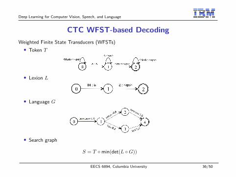
CTC WFST-based DecodingWeighted Finite State Transducers (WFSTs)• Token T
• Lexion L
• Language G
• Search graph
S = T ◦min(det(L ◦G))
EECS 6894, Columbia University 36/50

Deep Learning for Computer Vision, Speech, and Language
CTC Output Behavior
*A. Graves and N. Jaitly, "Towards End-to-End Speech Recognition with RecurrentNeural Networks", ICML, 2014. Adapted.
EECS 6894, Columbia University 37/50

Deep Learning for Computer Vision, Speech, and Language
Encoder-Decoder Architectures
Many-to-many sequence mapping.
EECS 6894, Columbia University 38/50
Deep Learning for Computer Vision, Speech, and Language
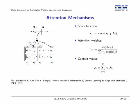
Attention Mechanisms• Score function:
eti = score(st−1,hi)
• Attention weights:
αti = exp(eti)∑Txj=1 exp(etj)
• Context vector:
ct =Tx∑i=1
αtihi
*D. Bahdanau, K. Cho and Y. Bengio, "Neural Machine Translation by Jointly Learning to Align and Translate",ICLR, 2015.
EECS 6894, Columbia University 39/50

Deep Learning for Computer Vision, Speech, and Language
Some Attention Functions
• Dot-Product-Attention
score(st−1,hi) = sTt−1Whi
• Additive-Attention
score(st−1,hi) = vTtanh(Wst−1 + Uhi + b)
• Location-Based-Attention
Ft = K ∗αt−1
score(st−1,hi) = vTtanh(Wst−1 + Uhi + VFt,i + b)
• Multi-Head-Attention
EECS 6894, Columbia University 40/50

Deep Learning for Computer Vision, Speech, and Language
Decoding in the Encoder-Decoder Architecture
• Decoder as a sequence generation model:I At each time stamp, the decoder generates a probability
distribution over the vocabulary
P (zt|zt−1, · · · , z1;x1, x2, · · · , xT)
I Draw a word from the vocabulary according to the distributionI Feed it as input to the next time stampI Repeat until an <EOS> shows up.
• The goal is to generate the most likely output word sequence• SolutionsI Simply picking the most likely word at each time stamp is
suboptimalI Keep multiple hypotheses and conduct the beam search
EECS 6894, Columbia University 41/50

Deep Learning for Computer Vision, Speech, and Language
Data Augmentation by Label Preserving Transformations
• Artificially augment the training set using replicas of trainingsamples under certain transformations.
• Make neural networks invariant to such transformations.
• Helpful when training data is limited.
• Some commonly-used approaches
I perturbation of speaking rateI perturbation of vocal tract lengthI voice conversion in some designated feature space by
stochastic mappingI multi-style training by adding noise
EECS 6894, Columbia University 42/50
Deep Learning for Computer Vision, Speech, and Language
Adaptation of Acoustic Models – Transfer Learning
• A classifier Pθ(Y |X)A training population distribution Ps(X)A test population distribution Pt(X)X ∈ Rn, Y ∈ Rm
• Pθ(Y |X) is learned from training data under distributionPs(X)
• Same Pθ(Y |X) is used for classification on test data underdistribution Pt(X)
• What happens if Ps(X) 6= Pt(X)?
EECS 6894, Columbia University 43/50

Deep Learning for Computer Vision, Speech, and Language
Distribution Mismatch In Transfer Learning
Ps(x) Pt(x)
EECS 6894, Columbia University 44/50

Deep Learning for Computer Vision, Speech, and Language
Why Adaptation Is Needed In Acoustic Modeling
• Speech signals are affected by a variety of variabilitiesI speakerI environmentI channelI . . . . . .
• An important issue to deal with in acoustic modelingI a test speech signal may come from a sparse region of the
training distribution, which may give rise to performancedegradation
I adaptation or adaptive training is constantly pursued tomitigate the distribution mismatch
EECS 6894, Columbia University 45/50

Deep Learning for Computer Vision, Speech, and Language
Adaptation of DNN-HMMs• What did we do in GMM-HMMs?I elegant mathematical models (MLLR, fMLLR, MAP,
eigenVoice, . . . . . . )I exploit the generative structure of GMM-HMM for parameter
tying
• What’s the challenge of adapting DNN-HMMs?I substantial number of parameters → data sparsity seems to
always be the issue for DNN adaptationI lack of a generative structure for parameter tyingI unsupervised adaptation, which is preferred in practice, makes
it even harder due to the strong discriminative nature of DNNs.I catastrophic forgetting
EECS 6894, Columbia University 46/50

Deep Learning for Computer Vision, Speech, and Language
Some Commonly-used Techniques for DNN Adaptation• Use speaker-adapted input features (e.g. fMLLR, VTL-warpedlogMEL)• Fine-tune the whole network with a small learning rate• Fine-tune or retrain a selected subset of the network parametersI input/output/hidden layer(s)I SVD factorization of the output layer (m>n, n�k)
Wm×n = Um×mΣm×nVTn×n ≈ Um×kΣk×kVT
n×k = Um×kNk×n
Wm×n = Um×kSk×kNk×n
• Learning hidden unit contributions (LHUC)
a(l)i =
∑j
w(l)ij z
(l−1)j + b(l)
i , z(l)i = γ(l)
i · σ(a(l)
i
)I motivated a family of parameterized activation functions
• Speaker-aware training based on i-vectors
x 7→ [x, e]
EECS 6894, Columbia University 47/50

Deep Learning for Computer Vision, Speech, and Language
Some Commonly-used Techniques for DNN Adaptation
EECS 6894, Columbia University 48/50

Deep Learning for Computer Vision, Speech, and Language
Multilingual Acoustic Modeling• Oftentimes, to build an ASR system, the acoustic resourcesfor a particular language or a particular domain is limited.
• Universal acoustic representations can significantly help thissituation.I mitigate sparse data issueI better performanceI faster system turn-around
• Multilingual acoustic modelingI Learning feature representations of universal acoustic
characteristics from numerous languagesI deep learning is especially suitable for multilingual acoustic
modeling
EECS 6894, Columbia University 49/50

Deep Learning for Computer Vision, Speech, and Language
A Case Study of Multilingual Feature Extraction• 24 languages under the IARPA Babel program• Cantonese, Assamese, Bengali, Pashto, Turkish, Tagalog, Vietnamese, Haitian Creole,
Swahili, Lao, Tamil, Kurmanji Kurdish, Zulu, Tok Pisin, Cebuano, Kazakh, Telugu,Lithuanian, Amharic, Dholuo, Guarani, Igbo, Javanese, Mongolian.• 40-70 hours of labeled speech data from each language.
EECS 6894, Columbia University 50/50
Related Documents


![Automatic Speech Recognition - folk.idi.ntnu.no · automatic speech recognition technology to appropriately route and handle the calls [3]. Speech recognition technology has also](https://static.cupdf.com/doc/110x72/5e3a689dba46991b3c2c91e9/automatic-speech-recognition-folkidintnuno-automatic-speech-recognition-technology.jpg)


