POLITECNICO DI MILANO Master’s Degree in Computer Science and Engineering Dipartimento di Elettronica, Informazione e Bioingegneria DEEP FEATURE EXTRACTION FOR SAMPLE-EFFICIENT REINFORCEMENT LEARNING Supervisor: Prof. Marcello Restelli Co-supervisors: Dott. Carlo D’Eramo, Dott. Matteo Pirotta Master’s Thesis by: Daniele Grattarola (Student ID 853101) Academic Year 2016-2017

Welcome message from author
This document is posted to help you gain knowledge. Please leave a comment to let me know what you think about it! Share it to your friends and learn new things together.
Transcript
POLITECNICO DI MILANOMaster’s Degree in Computer Science and Engineering
Dipartimento di Elettronica, Informazione e Bioingegneria
DEEP FEATURE EXTRACTION FOR
SAMPLE-EFFICIENT REINFORCEMENT
LEARNING
Supervisor: Prof. Marcello Restelli
Co-supervisors: Dott. Carlo D’Eramo, Dott. Matteo Pirotta
Master’s Thesis by:
Daniele Grattarola (Student ID 853101)
Academic Year 2016-2017


Il piu e fatto.


Contents
Abstract IX
Riassunto XI
Aknowledgments XVII
1 Introduction 1
1.1 Goals and Motivation . . . . . . . . . . . . . . . . . . . . . . . . . . . . 2
1.2 Proposed Solution . . . . . . . . . . . . . . . . . . . . . . . . . . . . . . 2
1.3 Original Contributions . . . . . . . . . . . . . . . . . . . . . . . . . . . . 3
1.4 Thesis Structure . . . . . . . . . . . . . . . . . . . . . . . . . . . . . . . 3
2 Background 5
2.1 Deep Learning . . . . . . . . . . . . . . . . . . . . . . . . . . . . . . . . 5
2.1.1 Artificial Neural Networks . . . . . . . . . . . . . . . . . . . . . . 6
2.1.2 Backpropagation . . . . . . . . . . . . . . . . . . . . . . . . . . . 7
2.1.3 Convolutional Neural Networks . . . . . . . . . . . . . . . . . . . 10
2.1.4 Autoencoders . . . . . . . . . . . . . . . . . . . . . . . . . . . . . 12
2.2 Reinforcement Learning . . . . . . . . . . . . . . . . . . . . . . . . . . . 13
2.2.1 Markov Decision Processes . . . . . . . . . . . . . . . . . . . . . 14
2.2.2 Optimal Value Functions . . . . . . . . . . . . . . . . . . . . . . 17
2.2.3 Value-based Optimization . . . . . . . . . . . . . . . . . . . . . . 18
2.2.4 Dynamic Programming . . . . . . . . . . . . . . . . . . . . . . . 19
2.2.5 Monte Carlo Methods . . . . . . . . . . . . . . . . . . . . . . . . 20
2.2.6 Temporal Difference Learning . . . . . . . . . . . . . . . . . . . . 21
2.2.7 Fitted Q-Iteration . . . . . . . . . . . . . . . . . . . . . . . . . . 24
2.3 Additional Formalism . . . . . . . . . . . . . . . . . . . . . . . . . . . . 25
2.3.1 Decision Trees . . . . . . . . . . . . . . . . . . . . . . . . . . . . 25
2.3.2 Extremely Randomized Trees . . . . . . . . . . . . . . . . . . . . 27
I

3 State of the Art 29
3.1 Value-based Deep Reinforcement Learning . . . . . . . . . . . . . . . . . 29
3.2 Other Approaches . . . . . . . . . . . . . . . . . . . . . . . . . . . . . . 32
3.2.1 Memory Architectures . . . . . . . . . . . . . . . . . . . . . . . . 32
3.2.2 AlphaGo . . . . . . . . . . . . . . . . . . . . . . . . . . . . . . . 33
3.2.3 Asynchronous Advantage Actor-Critic . . . . . . . . . . . . . . . 35
3.3 Related Work . . . . . . . . . . . . . . . . . . . . . . . . . . . . . . . . . 36
4 Deep Feature Extraction for Sample-Efficient Reinforcement Learning 37
4.1 Motivation . . . . . . . . . . . . . . . . . . . . . . . . . . . . . . . . . . 37
4.2 Algorithm Description . . . . . . . . . . . . . . . . . . . . . . . . . . . . 38
4.3 Extraction of State Features . . . . . . . . . . . . . . . . . . . . . . . . . 40
4.4 Recursive Feature Selection . . . . . . . . . . . . . . . . . . . . . . . . . 43
4.5 Fitted Q-Iteration . . . . . . . . . . . . . . . . . . . . . . . . . . . . . . 46
5 Technical Details and Implementation 47
5.1 Atari Environments . . . . . . . . . . . . . . . . . . . . . . . . . . . . . 47
5.2 Autoencoder . . . . . . . . . . . . . . . . . . . . . . . . . . . . . . . . . 50
5.3 Tree-based Recursive Feature Selection . . . . . . . . . . . . . . . . . . . 52
5.4 Tree-based Fitted Q-Iteration . . . . . . . . . . . . . . . . . . . . . . . . 53
5.5 Evaluation . . . . . . . . . . . . . . . . . . . . . . . . . . . . . . . . . . . 53
6 Experimental Results 55
6.1 Premise . . . . . . . . . . . . . . . . . . . . . . . . . . . . . . . . . . . . 55
6.2 Baseline . . . . . . . . . . . . . . . . . . . . . . . . . . . . . . . . . . . . 56
6.3 Autoencoder . . . . . . . . . . . . . . . . . . . . . . . . . . . . . . . . . 58
6.4 Recursive Feature Selection . . . . . . . . . . . . . . . . . . . . . . . . . 62
6.5 Fitted Q-Iteration . . . . . . . . . . . . . . . . . . . . . . . . . . . . . . 64
7 Conclusions and Future Developments 69
7.1 Future Developments . . . . . . . . . . . . . . . . . . . . . . . . . . . . . 70
References 73

List of Figures
1 Esempio di estrazione di feature con una CNN . . . . . . . . . . . . . . XII
2 Rappresentazione dei tre moduli principali . . . . . . . . . . . . . . . . . XIV
2.1 Graphical representation of the perceptron model . . . . . . . . . . . . . 6
2.2 A fully-connected neural network with two hidden layers . . . . . . . . . 7
2.3 Linear separability with perceptron . . . . . . . . . . . . . . . . . . . . . 8
2.4 Visualization of SGD on a space of two parameters . . . . . . . . . . . . 9
2.5 Effect of the learning rate on SGD updates . . . . . . . . . . . . . . . . 10
2.6 Shared weights in CNN . . . . . . . . . . . . . . . . . . . . . . . . . . . 11
2.7 CNN for image processing . . . . . . . . . . . . . . . . . . . . . . . . . . 11
2.8 Max pooling . . . . . . . . . . . . . . . . . . . . . . . . . . . . . . . . . . 12
2.9 Schematic view of an autoencoder . . . . . . . . . . . . . . . . . . . . . 12
2.10 Reinforcement learning setting . . . . . . . . . . . . . . . . . . . . . . . 14
2.11 Graph representation of an MDP . . . . . . . . . . . . . . . . . . . . . . 15
2.12 Policy iteration . . . . . . . . . . . . . . . . . . . . . . . . . . . . . . . . 19
2.13 Recursive binary partitioning . . . . . . . . . . . . . . . . . . . . . . . . 25
3.1 Structure of the Deep Q-Network by Mnih et al. . . . . . . . . . . . . . 30
3.2 Some of the games available in the Atari environments . . . . . . . . . . 31
3.3 Architecture of NEC . . . . . . . . . . . . . . . . . . . . . . . . . . . . . 33
3.4 Neural network training pipeline of AlphaGo . . . . . . . . . . . . . . . 34
3.5 The asynchronous architecture of A3C . . . . . . . . . . . . . . . . . . . 35
4.1 Schematic view of the three main modules . . . . . . . . . . . . . . . . . 39
4.2 Schematic view of the AE . . . . . . . . . . . . . . . . . . . . . . . . . . 42
4.3 Example of non-trivial nominal dynamics . . . . . . . . . . . . . . . . . 43
4.4 RFS on Gridworld . . . . . . . . . . . . . . . . . . . . . . . . . . . . . . 45
5.1 Sampling frames at a frequency of 14 in Breakout . . . . . . . . . . . . . 48
5.2 Two consecutive states in Pong . . . . . . . . . . . . . . . . . . . . . . . 49
5.3 The ReLU and Sigmoid activation functions for the AE . . . . . . . . . 51
III

6.1 Average performance of DQN in Breakout . . . . . . . . . . . . . . . . . 57
6.2 Average performance of DQN in Pong . . . . . . . . . . . . . . . . . . . 57
6.3 Average performance of DQN in Space Invaders . . . . . . . . . . . . . . 58
6.4 AE reconstruction and feature maps on Breakout . . . . . . . . . . . . . 59
6.5 AE reconstruction and feature maps on Pong . . . . . . . . . . . . . . . 60
6.6 AE reconstruction and feature maps on Space Invaders . . . . . . . . . . 60
6.7 Predictions of S-Q mapping experiment . . . . . . . . . . . . . . . . . . 63
6.8 RFS dependency tree in Breakout . . . . . . . . . . . . . . . . . . . . . 65
6.9 RFS dependency tree in Pong . . . . . . . . . . . . . . . . . . . . . . . . 66

List of Tables
5.1 Layers of the autoencoder with key parameters . . . . . . . . . . . . . . 49
5.2 Optimization hyperparameters for Adam . . . . . . . . . . . . . . . . . . 51
5.3 Parameters for Extra-Trees (RFS) . . . . . . . . . . . . . . . . . . . . . 51
5.4 Parameters for RFS . . . . . . . . . . . . . . . . . . . . . . . . . . . . . 52
5.5 Parameters for Extra-Trees (FQI) . . . . . . . . . . . . . . . . . . . . . . 53
5.6 Parameters for evaluation . . . . . . . . . . . . . . . . . . . . . . . . . . 54
6.1 Server configurations for experiments . . . . . . . . . . . . . . . . . . . . 56
6.2 Performance of baseline algorithms . . . . . . . . . . . . . . . . . . . . . 56
6.3 AE validation performance . . . . . . . . . . . . . . . . . . . . . . . . . 59
6.4 Results of S-Q mapping experiment . . . . . . . . . . . . . . . . . . . . 61
6.5 Feature selection results . . . . . . . . . . . . . . . . . . . . . . . . . . . 64
6.6 Performance of our algorithm . . . . . . . . . . . . . . . . . . . . . . . . 64
6.7 Performance of our algorithm w.r.t. the baselines . . . . . . . . . . . . . 67
6.8 Performance of our algorithm on small datasets . . . . . . . . . . . . . . 67
6.9 Sample efficiency of our algorithm . . . . . . . . . . . . . . . . . . . . . 67
V


List of Algorithms
1 SARSA . . . . . . . . . . . . . . . . . . . . . . . . . . . . . . . . . . . . 23
2 Q-Learning . . . . . . . . . . . . . . . . . . . . . . . . . . . . . . . . . . 23
3 Fitted Q-Iteration . . . . . . . . . . . . . . . . . . . . . . . . . . . . . . 24
4 Extra-Trees node splitting . . . . . . . . . . . . . . . . . . . . . . . . . . 28
5 Deep Q-Learning with Experience Replay . . . . . . . . . . . . . . . . . 31
6 Fitted Q-Iteration with Deep State Features . . . . . . . . . . . . . . . . 41
7 Recursive Feature Selection (RFS) . . . . . . . . . . . . . . . . . . . . . 43
8 Iterative Feature Selection (IFS) . . . . . . . . . . . . . . . . . . . . . . 46
VII


Abstract
Deep reinforcement learning (DRL) has been under the spotlight of artificial intelligence
research in recent years, enabling reinforcement learning agents to solve control problems
that were previously considered intractable. The most effective DRL methods, however,
require a great amount of training samples (in the order of tens of millions) in order to
learn good policies even on simple environments, making them a poor choice in real-
world situations where the collection of samples is expensive.
In this work, we propose a sample-efficient DRL algorithm that combines unsuper-
vised deep learning to extract a representation of the environment, and batch reinforce-
ment learning to learn a control policy using this new state space. We also add an
intermediate step of feature selection on the extracted representation in order to reduce
the computational requirements of our agent to the minimum. We test our algorithm
on the Atari games environments, and compare the performance of our agent to that of
the DQN algorithm by Mnih et al. [32]. We show that even if the final performance of
our agent amounts to a quarter of DQN’s, we are able to achieve good sample efficiency
and a better performance on small datasets.
IX


Riassunto
L’apprendimento profondo per rinforzo (in inglese deep reinforcement learning - DRL)
ha recentemente suscitato un grande interesse nel campo dell’intelligenza artificiale, per
la sua capacita senza precedenti nel risolvere problemi di controllo considerati fino ad
ora inavvicinabili. A partire dalla pubblicazione dell’algoritmo deep Q-learning (DQN)
di Mnih et al. [32], il campo dell’apprendimento per rinforzo ha vissuto un vero e proprio
rinascimento, caratterizzato da un susseguirsi di pubblicazioni con algoritmi di controllo
sempre piu efficaci nel risolvere ambienti ad alta dimensionalita, con prestazioni simili
o superiori agli esseri umani. Tuttavia, una caratteristica comune agli algoritmi di
DRL e la necessita di utilizzare un enorme numero di campioni di addestramento per
arrivare a convergenza. Alcune delle pubblicazioni piu recenti cercano di affrontare la
problematica, riuscendo pero ad abbassare questo numero al massimo di un ordine di
grandezza.
Lo scopo di questa tesi e presentare un algoritmo di DRL che riesca ad apprendere
politiche di controllo soddisfacenti in ambienti complessi, utilizzando solo una frazio-
ne dei campioni necessari agli algoritmi dello stato dell’arte. Il nostro agente utilizza
l’apprendimento profondo non supervisionato per estrarre una rappresentazione astratta
dell’ambiente, e l’apprendimento per rinforzo in modalita batch per ricavare una politica
di controllo a partire da questo nuovo spazio degli stati. Aggiungiamo, inoltre, una pro-
cedura di selezione delle feature applicata alla rappresentazione estratta dall’ambiente,
in modo da ridurre al minimo i requisiti computazionali del nostro agente.
In fase sperimentale, applichiamo il nostro algoritmo ad alcuni ambienti di test dei
sopracitati giochi Atari, confrontandolo con DQN. Come risultato principale, mostriamo
che il nostro agente e in grado di raggiungere in media un quarto dei punteggi ottenuti
da DQN sugli stessi ambienti, ma utilizzando circa un centesimo dei campioni di adde-
stramento. Mostriamo inoltre che, a parita di campioni raccolti dal nostro algoritmo per
raggiungere le migliori prestazioni, i punteggi ottenuti dal nostro agente sono in media
otto volte piu alti di quelli di DQN.
XI

Figura 1: Esempio di estrazione gerarchica di feature con una CNN.
Apprendimento Profondo
L’apprendimento profondo (normalmente noto con il termine inglese deep learning) e
una tecnica di apprendimento automatico utilizzata per estrarre rappresentazioni astrat-
te del dominio. I metodi profondi si basano su molteplici livelli di rappresentazio-
ne, ottenuti dalla composizione di moduli semplici, ma non lineari, che trasformano la
rappresentazione ricevuta in ingresso in una rappresentazione leggermente piu astratta.
Il deep learning e alla base della ricerca moderna in apprendimento automatico, ed
i risultati piu impressionanti sono stati tipicamente raggiunti grazie alla versatilita del-
le reti neurali. Oltre ad essere un potente approssimatore universale, questo semplice
modello ispirato alla struttura interconnessa del cervello biologico si presta alla composi-
zione gerarchica, rendendolo un blocco ideale per l’apprendimento profondo. Gran parte
dei progressi nel campo del deep learning sono dovuti alle reti neurali convoluzionali (in
inglese convolutional neural networks - CNN), ispirate al funzionamento della corteccia
visiva del cervello (Figura 1). Le CNN sono state applicate con notevole successo a
svariati problemi, dalla visione artificiale [26, 42] alla traduzione automatica [48], e si
basano sull’utilizzo di filtri che vengono fatti scorrere sull’ingresso ad ogni livello, per in-
dividuare correlazioni spaziali locali che caratterizzino il dominio. L’efficacia delle CNN
deriva proprio da questa natura intrinsecamente spaziale, che consente di processare
domini complessi (come le immagini) con un’ottima generalita.

Deep Reinforcement Learning
Il deep reinforcement learning (DRL) e una branca dell’apprendimento per rinforzo che
utilizza approssimatori ad apprendimento profondo per estrarre una rappresentazione
astratta dell’ambiente, e utilizza poi questa rappresentazione per apprendere una poli-
tica di controllo ottimale. Il DRL ha causato una vera e propria rivoluzione nel campo
dell’intelligenza artificiale, e la letteratura sulla materia ha visto un incremento esponen-
ziale delle pubblicazioni. Tra queste, citiamo nuovamente l’algoritmo che ha innescato
l’interesse nel DRL, DQN di Mnih et al. [32], e i derivati di DQN proposti da Van Hasselt
et al. (2016) [20] con Double DQN (DDQN), Schaul et al. (2016) [38] con prioritized expe-
rience replay e Wang et al. (2016) [45] con dueling architecture. Altri approcci proposti
nella letteratura di DRL includono l’algoritmo Asynchronous Advantage Actor-Critic
(A3C) di Mnih et al. (2016) [31] caratterizzato da un’ottima velocita di apprendimento,
il programma AlphaGo di Silver et al. (2016) [39] in grado di sconfiggere il campione
del mondo Ke Jie nel complicato gioco da tavolo del Go, e Neural Episodic Control di
Pritzel et al. (2017) [36], che al momento della stesura di questa tesi costituisce lo stato
dell’arte per l’apprendimento sui famosi Atari games.
La tipica applicazione del DRL consiste nel risolvere problemi di controllo a partire
dalla rappresentazione visiva dell’ambiente. Questa configurazione consente di sfruttare
l’enorme capacita descrittiva delle CNN e permette di affrontare problemi complessi
senza la necessita di ingegnerizzare i descrittori dell’ambiente.
Feature Profonde per l’Apprendimento Efficiente
Come argomento centrale di questa tesi presentiamo un algoritmo di deep reinforcement
learning che combina:
• l’apprendimento profondo non supervisionato, per estrarre una rappresentazione
dell’ambiente;
• un algoritmo per la selezione di feature orientato al controllo, per ridurre al minimo
i requisiti computazionali dell’agente;
• un algoritmo di apprendimento per rinforzo in modalita batch, per apprendere una
politica a partire dalla rappresentazione prodotta dagli altri due moduli.
Lo scopo principale della procedura presentata e quello di apprendere una politica di
controllo efficace su un ambiente complesso, utilizzando il minor numero possibile di
campioni di addestramento.
Per l’estrazione di feature dall’ambiente, utilizziamo un autoencoder (AE) convo-
luzionale. L’AE e una forma di rete neurale che viene utilizzata per apprendere una

Figura 2: Rappresentazione schematica della composizione dei tre moduli, con le rispettive
trasformazioni evidenziate in alto.
rappresentazione del dominio in maniera non supervisionata, costituita da due modu-
li separati: un encoder e un decoder. Lo scopo dell’encoder e semplicemente quello
di estrarre una rappresentazione compressa degli ingressi, mentre quello del decoder e
di invertire questa trasformazione e ricostruire l’ingresso originale a partire dalla com-
pressione prodotta dall’encoder. I due componenti vengono addestrati come un’unica
rete neurale, propagando il gradiente su tutti i pesi contemporaneamente. Al termine
dell’apprendimento, l’encoder viene utilizzato per comprimere gli elementi del domi-
nio, idealmente implementando una forma di compressione senza perdita che riduca la
dimensionalita dello spazio di ingresso. Identifichiamo questa compressione come la tra-
sformazione ENC : S → S, dallo spazio degli stati originali S, allo spazio delle feature
astratte S.
Il secondo modulo della nostra catena di addestramento e l’algoritmo Recursive Fea-
ture Selection (RFS) di Castelletti et al. [8]. Questa procedura di selezione delle feature
utilizza l’apprendimento supervisionato per ordinare le feature di stato di un ambiente
in base alla loro utlita per il controllo, e riduce la dimensionalita del dominio rimuo-
vendo le feature meno utili a questo fine. Nel nostro caso, utilizziamo RFS per ridurre
ulteriormente la rappresentazione estratta dall’AE, in modo da ottenere uno spazio delle
feature minimale ed essenziale per il controllo. Anche in questo caso, il prodotto del
modulo e una trasformazione RFS : S → S, dove S identifica lo spazio ridotto.
Infine, utilizziamo l’algoritmo di apprendimento per rinforzo batch Fitted Q-Iteration
(FQI) [11] per apprendere una politica di controllo per l’ambiente a partire da una
raccolta di transizioni (s, a, r, s�) (stato, azione, rinforzo, stato prossimo), dove s, s� ∈ S.
Alla fine dell’addestramento, l’algoritmo produce un approssimatore della funzione di
valore di azione Q : S ×A → R, dove A e lo spazio delle azioni.
I tre moduli vengono addestrati in sequenza per produrre le rispettive trasformazioni,

e alla fine della fase di addestramento vengono combinati per poter utilizzare la funzione
Q prodotta da FQI a partire dallo spazio degli stati originale (Figura 2). La sequenza di
addestramento, poi, viene ripetuta all’interno di un ciclo principale, che sequenzialmente
raccoglie un insieme di campioni su cui addestrare i tre moduli, utilizzando una politica
a tasso di esplorazione decrescente in modo da sfruttare sempre di piu la conoscenza
appresa dall’agente, fino a convergenza. Ogni sequenza di addestramento e seguita da
una fase di valutazione, per stabilire se le prestazioni dell’agente siano soddisfacenti ed
eventualmente terminare la procedura.
Esperimenti e Conclusioni
Nella fase sperimentale applichiamo l’algoritmo a tre ambienti dei giochi Atari, e per
valutare le prestazioni del nostro agente le compariamo a quelle ottenute da DQN di
Mnih et al. [32] sugli stessi giochi.
Osserviamo che l’AE riesce ad ottenere un’ottima precisione nella ricostruzione dello
spazio originale degli stati, e che le feature estratte dall’encoder sono sufficientemente
astratte. Per verificare la qualita delle feature al fine del controllo, addestriamo un mo-
dello supervisionato per approssimare la funzione Q appresa da DQN, a partire dalle
feature prodotte dall’AE. L’alto coefficiente di correlazione dei valori predetti in vali-
dazione conferma che le feature estratte sono adatte al controllo, o che quantomeno
contengono tutta l’informazione necessaria a stimare le funzioni di valore ottime degli
ambienti.
A causa degli enormi requisiti di potenza computazionale, possiamo condurre pochi
esperimenti relativi a RFS, e siamo costretti a rimuoverlo completamente dalla catena
di addestramento per valutare le prestazioni finali dell’agente in tempi trattabili. I
tre esperimenti che portiamo a termine (uno per ogni ambiente), producono risultati
variabili e inaspettati, e ci portano a rimandare l’analisi della procedura di selezione ad
un secondo momento.
Infine, la valutazione dell’algoritmo completo conferma il raggiungimento dell’obiet-
tivo di efficienza e sottolinea un grande potenziale della procedura, che tuttavia non
riesce ad arrivare alle stesse prestazioni dello stato dell’arte. Il nostro agente riesce ad
ottenere in media il 25% del punteggio di DQN, utilizzando pero lo 0.3% dei campioni di
addestramento richiesti in media da DQN per raggiungere la miglior prestazione. Allo
stesso tempo, valutando i punteggi raggiunti da entrambi gli algoritmi limitandosi a que-
sto numero di campioni estremamente ridotto, osserviamo che il nostro agente ottiene
punteggi mediamente superiori di otto volte rispetto a quelli di DQN, che necessita di un
numero dieci volte piu grande di esempi per imparare una politica equivalente. Il nostro
algoritmo dimostra dunque una grande efficienza nell’utilizzo dei campioni, rendendolo
adatto al controllo in situazioni in cui la raccolta di campioni e difficile o costosa.


Acknowledgments
All the work presented in this thesis was done under the supervision of Prof. Marcello
Restelli, who has instilled in me the passion for this complex and fascinating subject and
helped me navigate it since the beginning. I also thank Dott. Carlo D’Eramo for guiding
me during my first steps into the academic world and inspiring me to pursue a career
in research, and Dott. Matteo Pirotta for providing useful insights and supervision on
this work.
It is impossible to summarize the unique experience I had at PoliMi in a few para-
graphs, but I would like to thank Ilyas Inajjar, Giacomo Locci, Angelo Gallarello, Davide
Conficconi, Alessandro Comodi, Francesco Lattari, Edoardo Longo, Stefano Longari,
Yannick Giovanakis, Paolo Mosca and Andrea Lui for sharing their experiences with me
and always showing me a different perspective of the things we do. I thank Politecnico
di Milano for providing the infrastructure during my education and the writing of this
thesis, but most importantly for fostering a culture of academic excellence, of collabo-
ration, and of passion for the disciplines of its students. I also thank Prof. Cremonesi
and Prof. Alippi for giving me a chance to prove myself.
Finally, this thesis is dedicated to my parents, for giving me all that I am and all
that I have; to Gaia, for being the reason to always look ahead; to my grandmothers,
for their unconditional love; to my grandfather, for always rooting silently.
XVII


Chapter 1
Introduction
Human behavior is a complex mix of elements. We are subject to well defined biolog-
ical and social forces, but at the same time our actions are deliberate, our thinking is
abstract, and our objectives can be irrational; our brains are extremely complex inter-
connections, but of extremely simple building blocks; we are crafted by ages of random
evolution, but at the same time of precise optimization. When we set out to describe the
inner workings of human cognition, we must consider all of these colliding aspects and
account for them in our work, without overcomplicating what is simple or approximating
what is complex.
Artificial intelligence is a broad field, that looks at the variegate spectrum of hu-
man behavior to replicate our complexity in a formal or algorithmic way. Among the
techniques of AI, one family of algorithms called machine learning is designed to give
computers the ability to learn to carry out a task without being explicitly programmed
to do so. The focus on different types of tasks is what defines the many subfields of
machine learning. For instance, the use of machine learning algorithms to take decisions
in a sequential decision-making problem is called reinforcement learning, whereas deep
learning is a family of techniques to learn an abstract representation of a vector space
(e.g. learning how to describe an image from the value of its pixels).
Teaching machines to behave like human beings is a complex and inspiring problem
on its own; however, an even more complex task is not to simply teach computers to
mimic humans, but to do so with the same learning efficiency of the biological brain,
which is able to solve problems by experiencing them very few times (sometimes even
imagining a problem is enough to solve it, by comparing it with other similar known
situations). The purpose of this thesis is to make a step in this direction by combining
powerful machine learning techniques with efficient ones, in order to tackle complex
control problems without needing many examples to learn from.

1.1 Goals and Motivation
The source of inspiration for this work comes from the recent progress in reinforcement
learning associated to deep reinforcement learning (DRL) techniques. Among these, we
cite Deep Q-Learning by Mnih et al. [32], the Asynchronous Advantage Actor-Critic
algorithm also by Mnih et al. [31], and the Neural Episodic Control algorithm by Pritzel
et al. [36]. All these algorithms (which were all the state of the art at the time of their
respective publication), are based on deep learning to extract the visual characteristics
of an environment, and then using those characteristics to learn a policy with well-known
reinforcement learning techniques. A major drawback of these approaches, however, is
that they all require an enormous amount of experience to converge, which may prove
unfeasible in real-world problems where the collection of examples is expensive. The
main purpose of this work is to explore the limits of this apparent requirement, and to
propose an algorithm that is able to perform well even under such scarcity conditions.
1.2 Proposed Solution
We introduce a deep reinforcement learning agent that extracts an abstract descrip-
tion of the environment starting from its visual characteristics, and then leverages this
description to learn a complex behavior using a small collection of training examples.
We devise a combination of different machine learning techniques. We use unsu-
pervised deep learning to extract a representation of the visual characteristics of the
environment, as well as a feature selection procedure to reduce this representation while
keeping all the necessary information for control, and a batch reinforcement learning
algorithm which exploits this filtered representation to learn a policy. The result is a
reinforcement learning procedure that requires a small amount of experience in order to
learn, and which produces an essential and general representation of the environment
as well as a well-performing control policy for it.
We test our algorithm on the Atari games environments, which are the de facto
standard test bench of deep reinforcement learning, and we also perform an experimental
validation of all the components in our learning pipeline in order to ensure the quality
of our approach. We test the suitability of the extracted representation to both describe
the environment and provide all the information necessary for control, as well as we gain
useful knowledge on some environments by looking at the feature selection.
We compare our results with the DQN algorithm by Mnih et al. [32], and we find
that our agent is able to learn non-trivial policies on the tested environments, but that it
fails to converge to the same performance of DQN. However, we show that the number of
samples required by our procedure to reach its maximum performance is up to two orders
of magnitude smaller than that required by DQN, and that our agent’s performance is
on average eight times higher when limiting the training of the two methods to this
2

small number of samples.
1.3 Original Contributions
The use of unsupervised deep learning to extract a feature space for control purposes
had already been proposed by Lange and Riedmiller (2010) [27] before the field of deep
reinforcement learning really took off in the early 2010s. However, their approach used
a different architecture for the feature extraction, which would be inefficient for complex
control problems like the ones we test in this work.
Moreover, to the best of our knowledge there is no work in the literature that applies
a feature selection technique explicitly targeted for control purposes to deep features.
This additional step allows us to optimize our feature extraction process for obtaining
a generic description of the environment rather than a task-specific one, while at the
same time improving the computational requirements of our agent by keeping only the
essential information.
Our algorithm makes a step towards a more sample-efficient deep reinforcement
learning, and would be a better pick than DQN in situations characterized by a lack of
training samples and a big state space.
1.4 Thesis Structure
The thesis is structured as follows.
In Chapter 2 we provide the theoretical framework on which our algorithm is based,
and we give an overview of the most important concepts and techniques in the fields of
deep learning and reinforcement learning.
In Chapter 3 we summarize the state-of-the-art results in the field of deep reinforce-
ment learning.
In Chapter 4 we introduce our deep reinforcement learning algorithm, and provide
a formal description of its components and their behavior.
In Chapter 5 we describe in detail the specific implementation of each module in the
algorithm, with architectural choices, model hyperparameters, and training configura-
tions.
In Chapter 6 we show experimental results from running the algorithm on different
environments.
In Chapter 7 we summarize our work and discuss possible future developments and
improvements.
3

4

Chapter 2
Background
In this chapter we outline the theoretical framework that will be used in the following
chapters. The approach proposed in this thesis draws equally from the fields of deep
learning and reinforcement learning, in a hybrid setting usually called deep reinforcement
learning.
In the following sections we give high level descriptions of these two fields, in order
to introduce a theoretical background, a common notation, and a general view of some
of the most important techniques in each area.
2.1 Deep Learning
Deep Learning (DL) is a branch of machine learning that aims to learn abstract represen-
tations of the input space by means of complex function approximators. Deep learning
methods are based on multiple levels of representation, obtained by composing simple
but nonlinear modules that each transform the representation at one level (starting with
the raw input) into a representation at a higher, slightly more abstract level [28].
Deep learning is at the heart of modern machine learning research, where deep models
have revolutionized many fields like computer vision [26, 42], machine translation [48]
and speech synthesis [44]. Generally, the most impressive results of deep learning have
been achieved through the versatility of neural networks, which are universal function
approximators well suited for hierarchical composition.
In this section we give a brief overview of the basic concepts behind deep neural
networks and introduce some important ideas that will be used in later chapters of this
thesis.
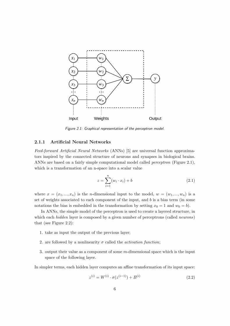
Figure 2.1: Graphical representation of the perceptron model.
2.1.1 Artificial Neural Networks
Feed-forward Artificial Neural Networks (ANNs) [5] are universal function approxima-
tors inspired by the connected structure of neurons and synapses in biological brains.
ANNs are based on a fairly simple computational model called perceptron (Figure 2.1),
which is a transformation of an n-space into a scalar value
z =
n�
i=1
(wi · xi) + b (2.1)
where x = (x1, ..., xn) is the n-dimensional input to the model, w = (w1, ..., wn) is a
set of weights associated to each component of the input, and b is a bias term (in some
notations the bias is embedded in the transformation by setting x0 = 1 and w0 = b).
In ANNs, the simple model of the perceptron is used to create a layered structure, in
which each hidden layer is composed by a given number of perceptrons (called neurons)
that (see Figure 2.2):
1. take as input the output of the previous layer;
2. are followed by a nonlinearity σ called the activation function;
3. output their value as a component of some m-dimensional space which is the input
space of the following layer.
In simpler terms, each hidden layer computes an affine transformation of its input space:
z(i) = W (i) · σ(z(i−1)) +B(i) (2.2)
6

Figure 2.2: A fully-connected neural network with two hidden layers.
where W (i) is the composition of the weights associated to each neuron in the layer and
B is the equivalent composition of the biases.
The processing of the input space performed by the sequence of layers that compose
an ANN is equivalent to the composition of multiple nonlinear transformations, which
results in the production of an output vector on the co-domain of the target function.
2.1.2 Backpropagation
Training ANNs is a parametric learning problem, where a loss function is minimized
starting from a set of training samples collected from the real process which is being
approximated. In parametric learning the goal is to find the optimal parameters of a
mathematical model, such that the expected error made by the model on the training
samples is minimized. In ANNs, the parameters that are optimized are the weight
matrices W (i) and biases B(i) associated to each hidden layer of the network.
In the simple perceptron model, which basically computes a linear transformation
of the input, the optimal parameters are learned from the training set according to the
following update rule:
wnewi = wold
i − η(y − y)xi, ∀i = (1, ..., n) (2.3)
where y is the output of the perceptron, y is the real target from the training set, xi is
the i-th component of the input, and η is a scaling factor called the learning rate which
regulates how much the weights are allowed to change in a single update. Successive
7

Figure 2.3: Different classification problems on a two-dimensional space, respectively linearly, non-
linearly and non separable. The perceptron would be able to converge and correctly classify the points
only in the first setting.
applications of the update rule for the perceptron guarantee convergence to an optimum
if and only if the approximated function is linear (in the case of regression) or the
problem is linearly separable (in the case of classification) as shown in Figure 2.3.
The simple update rule of the perceptron, however, cannot be used to train an ANN
with multiple layers because the true outputs of the hidden layers are not known a priori.
To solve this issue, it is sufficient to notice that the function computed by each layer of a
network is nonlinear, but differentiable with respect to the layer’s input (i.e. it is linear
in the weights). This simple fact allows to compute the partial derivative of the loss
function for each weight matrix in the network to, in a sense, impute the error committed
on a training sample proportionally across neurons. The error is therefore propagated
backwards (hence the name backpropagation) to update all weights in a similar fashion
to the perceptron update. The gradient of the loss function is then used to change
the value of the weights, with a technique called gradient descent which consists in the
following update rule:
Wnewi = W old
i − η∂L(y, y)
∂W oldi
(2.4)
where L is any differentiable function of the target and predicted values that quantifies
the error made by the model on the training samples. The term gradient descent is due
to the fact that the weights are updated in the opposite direction of the loss gradient,
moving towards a set of parameters for which the loss is lower (see Figure 2.4).
Notice that traditional gradient descent optimizes the loss function over all the train-
ing set at once, performing a single update of the parameters. This approach, however,
can be computationally expensive when the training set is big; a more common approach
is to use stochastic gradient descent (SGD) [5], which instead performs sequential pa-
rameters updates using small subsets of the training samples (called batches). As the
8

Figure 2.4: Visualization of SGD on a space of two parameters.
number of samples in a batch decreases, the variance of the updates increases, because
the error committed by the model on a single sample can have more impact on the gra-
dient step. This can cause the optimization algorithm to miss a good local optima due
to excessively big steps, but at the same time could help leaving a poor local minimum
in which the optimization is stuck. The same applies to the learning rate, which is the
other important factor in controlling the size of the gradient step: if the learning rate is
too big, SGD can overshoot local minima and fail to converge, but at the same time it
may take longer to find the optimum if the learning rate is too small (Figure 2.5).
In order to improve the accuracy and speed of SGD, some particular tweaks are
usually added to the optimization algorithm. Among these, we find the addition of a
momentum term to the update step of SGD, in order to avoid oscillating in irrelevant
directions by incorporating a fraction of the previous update term in the current one:
W(j+1)i = W
(j)i − γη
∂L(y(j−1), y(j−1))
∂W(j−1)i
− η∂L(y(j), y(j))
∂W(j)i
(2.5)
where (j) is the number of updates that have occurred so far. In this approach, momen-
tum has the same meaning as in physics, like when a body falling down a slope tends
to preserve part of its previous velocity when subjected to a force. Other techniques to
improve convergence include the use of an adaptive learning rate based on the previous
gradients computed for the weights (namely the Adagrad [9] and Adadelta [49] opti-
mization algorithms), and a similar approach which uses an adaptive momentum term
(called Adam [25]).
9

Figure 2.5: Effect of the learning rate on SGD updates. Too small (left) may take longer to converge,
too big (right) may overshoot the optimum and even diverge.
2.1.3 Convolutional Neural Networks
Convolutional Neural Networks (CNNs) are a type of ANN inspired by the visual cortex
in animal brains, and have been widely used in recent literature to reach state-of-the-art
results in fields like computer vision, machine translation, and, as we will see in later
sections, reinforcement learning.
CNNs exploit spatially-local correlations in the neurons of adjacent layers by using
a receptive field, a set of weights which is used to transform a local subset of the input
neurons of a layer. The receptive field is applied as a filter over different locations of
the input, in a fashion that resembles how a signal is strided across the other during
convolution. The result of this operation is a nonlinear transformation of the input
space into a new space (of compatible dimensions) that preserves the spatial information
encoded in the input (e.g. from the n×m pixels of a grayscale image to a j × k matrix
that represents subgroups of pixels in which there is an edge).
While standard ANNs have a fully connected (sometimes also called dense) structure,
with each neuron of a layer connected to each neuron of the previous and following layer,
in CNNs the weights are associated to a filter and shared across all neurons of a layer, as
shown in Figure 2.6. This weights sharing has the double advantage of greatly reducing
the number of parameters that must be updated during training, and of forcing the
network to learn general abstractions of the input that can be applied to any subset of
neurons covered by the filter.
In general, the application of a filter is not limited to one per layer and it is customary
to have more than one filter applied to the same input in parallel, to create a set of
independent abstractions called feature maps (also referred to as channels, to recall the
terminology of RGB images for which a 3-channel representation is used for red, green,
10

Figure 2.6: Simple representation of shared weights in a 1D CNN. Each neuron in the second layer
applies the same receptive field of three weights to three adjacent neurons of the previous layer. The
filter is applied with a stride of one element to produce the feature map.
Figure 2.7: Typical structure of a deep convolutional neural network for image processing, with two
convolutional hidden layers and a dense section at the end (for classification or regression).
and blue). In this case, there will be a set of shared weights for each filter. When a set
of feature maps is given as input to a convolutional layer, a multidimensional filter is
strided simultaneously across all channels.
At the same time, while it may be useful to have parallel abstractions of the input
space (which effectively enlarges the output space of the layers), it is also necessary
to force a reduction of the input in order to learn useful representations. For this
reason, convolutional layers in CNNs are often paired with pooling layers that reduce
the dimensionality of their input according to some criteria applied to subregions of the
input neurons (e.g. for each two by two square of input neurons, keep only the maximum
activation value as shown in Figure 2.8).
Finally, typical applications of CNNs in the literature use mixed architectures com-
posed of both convolutional and fully connected layers (Figure 2.7). In tasks like image
classification [40, 42], convolutional layers are used to extract significant features directly
from the images, and dense layers are used as a final classification model; the training in
this case is done in an end-to-end fashion, with the classification error being propagated
11

Figure 2.8: Example of max pooling, where only the highest activation value in the pooling window
is kept.
Figure 2.9: Schematic view of an autoencoder, with the two main components represented separately.
across all layers to fine-tune all weights and filters to the specific problem.
2.1.4 Autoencoders
Autoencoders (AE) are a type of ANN which is used to learn a sparse and compressed
representation of the input space, by sequentially compressing and reconstructing the
inputs under some sparsity constraint.
The typical structure of an AE is split into two sections: an encoder and a decoder
(Figure 2.9). In the classic architecture of autoencoders these two components are exact
mirrors of one another, but in general the only constraint that is needed to define an
AE is that the dimensionality of the input be the same as the dimensionality of the
output. In general, however, the last layer of the encoder should output a reduced
representation of the input which contains enough information for the decoder to invert
the transformation.
The training of an AE is done in an unsupervised fashion, with no explicit target
required as the network is simply trained to predict its input. Moreover, a strong
12

regularization constraint is often imposed on the innermost layer to ensure that the
learned representation is as abstract as possible (typically the L1 norm of the activations
is minimized as additional term to the loss, to enforce sparsity).
Autoencoders can be especially effective in extracting meaningful features from the
input space, without tailoring the features to a specific problem like in the end-to-end
image classification example of Section 2.1.3 [10]. An example of this is the extraction
of features from images, where convolutional layers are used in the encoder to obtain
an abstract description of the image’s structure. In this case, the decoder uses convo-
lutional layers to transform subregions of the representation, but the expansion of the
compressed feature space is delegated to upscaling layers (the opposite of pooling layers)
[30]. This approach in building the decoder, however, can sometimes cause blurry or
inaccurate reconstructions due to the upscaling operation which simply replicates in-
formation rather than transforming it (like pooling layers do). Because of this, a more
sophisticated technique has been developed recently which allows to build purely convo-
lutional autoencoders, without the need of upscaling layers in the decoder. The layers
used in this approach are called deconvolutional1 and are thoroughly presented in [50].
For the purpose of this thesis it suffices to notice that image reconstruction with this
type of layer is incredibly more accurate, down to pixel-level accuracy.
2.2 Reinforcement Learning
Reinforcement Learning (RL) is an area of machine learning that studies how to optimize
the behavior of an agent in an environment, in order to maximize the cumulative sum of
a scalar signal called reward in a setting of sequential decision making. RL has its roots
in optimization and control theory but, because of the generality of its characteristic
techniques, it has been applied to a variety of scientific fields where the concept of
optimal behavior in an environment can be applied (examples include game theory,
multi-agent systems and economy). The core aspect of reinforcement learning problems
is to represent the setting of an agent performing decisions in an environment, which
is in turn affected by the decisions; a scalar reward signal represents a time-discrete
indicator of the agent’s performance. This kind of setting is inspired to the natural
behavior of animals in their habitat, and the techniques used in reinforcement learning
are well suitable to describe, at least partially, the complexity of living beings.
In this section we introduce the basic setting of RL and go over a brief selection of
the main techniques used to solve RL problems.
1Or transposed convolutions.
13

Figure 2.10: The reinforcement learning setting, with the agent performing actions on the environ-
ment and in turn observing the state and reward.
2.2.1 Markov Decision Processes
Markov Decision Processes (MDPs) are discrete-time, stochastic control processes, that
can be used to describe the interaction of an agent with an environment (Figures 2.10
and 2.11).
Formally, MDPs are defined as 7-tuples < S, ST , A, P,R, γ, µ >, where:
• S is the set of observable states of the environment. When the set if observable
states coincides with the true set of states of the environment, the MDP is said
to be fully observable. We will only deal with fully observable MDPs without
considering the case of partially observable MDPs.
• ST ⊆ S is the set of terminal states of the environment, meaning those states in
which the interaction between the agent and the environment ends. The sequence
of events that occur from when the agent observes an initial state until it reaches
a terminal state is usually called episode.
• A is the set of actions that the agent can execute in the environment.
• P : S×A×S → [0, 1] is a state transition function which, given two states s, s� ∈ S
and an action a ∈ A, represents the probability of the agent going to state s� byexecuting a in s.
• R : S × A → R is a reward function which represents the reward that the agent
collects by executing an action in a state.
• γ ∈ [0, 1] is a discount factor which is used to weight the importance of rewards
during time: γ = 0 means that only the immediate reward is considered, γ = 1
means that all rewards have the same importance.
14

Figure 2.11: Graph representation of an MDP. Each gray node represents a state, each arc leaving a
state is associated to an action and its corresponding reward, an the action is in turn associated to
the following state; note that actions may have probability distributions over the outgoing arcs.
• µ : S → [0, 1] is a probability distribution over S which models the probability of
starting an episode in a given state.
Episodes are usually represented as sequences of tuples
[(s0, a0, r1, s1), ..., (sn−1, an−1, rn, sn)]
called trajectories, where s0 ∼ µ, sn ∈ ST , and (si, ai, ri+1, si+1) represents a transition
of the agent to state si+1 by taking action ai in si and collecting a reward ri+1.
In MDPs the modeled environment must satisfy the Markov property, meaning that
the reward and transition functions of the environment must only depend on the current
state and action, and not on the past state-action trajectory of the agent. In other words,
an environment is said to satisfy the Markov property when its one-step dynamics allow
to predict the next state and reward given only the current state and action.
Policy
The behavior of the agent in an MDP can be defined as a probability distribution
π : S × A → [0, 1] called a policy, which given s ∈ S and a ∈ A, represents the
probability of selecting a as next action from s. An agent that uses this probability
distribution to select its next action when in a given state is said to be following the
policy.
A common problem when defining policies is the exploration-exploitation dilemma.
An agent following a policy may end up observing the same trajectories in all episodes
(e.g. when following a deterministic policy in a deterministic MDP), but there may
be cases in which a better behavior could be had if the agent explored other states
15

instead of simply exploiting its knowledge. It is therefore common to add a probabilistic
element to policies (irrespectively of their determinism), in order to explicitly control
the exploration degree of the agent. Common techniques to control the exploration-
exploitation trade-off are:
• ε-greedy policies, in which actions are selected using a given policy with probability
1− ε, and randomly the rest of the time;
• softmax action selection, that improves on ε-greedy policies by reducing the num-
ber of times a suboptimal action is randomly selected. To do so, a probability
distribution (commonly a Boltzmann distribution) dependent on the expected re-
turn from the successor states (something called the value of the states, which we
introduce in the next subsection) is used.
Value Functions
Starting from the concept of policy, we can now introduce a function that evaluates how
good it is for an agent following a policy π to be in a given state. This evaluation is
expressed in terms of the expected return, i.e. the expected discounted sum of future
rewards collected by an agent starting from a state while following π, and the function
that computes it is called the state-value function for policy π (or, more commonly, just
value function).
Formally, the state-value function associated to a policy π is a function V π : S → Rdefined as:
V π(s) = Eπ[Rt|st = s] (2.6)
= Eπ[
∞�
k=0
γkrt+k+1|st = s] (2.7)
where Eπ[·] is the expected value given that the agent follows policy π, and t is any time
step of an episode [s0, ..., st, ..., sn] where st ∈ S, ∀t = 0, ..., n.
Similarly, we can also introduce a function that evaluates the goodness of taking
a specific action in a given state, namely the expected reward obtained by taking an
action a ∈ A in a state s ∈ S and then following policy π. We call this function the
action-value function for policy π denoted Qπ : S ×A → R, and defined as:
Qπ(s, a) = Eπ[Rt|st = s, at = a] (2.8)
= Eπ[∞�
k=0
γkrt+k+1|st = s, at = a] (2.9)
The majority of reinforcement learning algorithms is based on computing (or estimating)
the value functions, which can then be used to control the behavior of the agent. We also
16

note a fundamental property of the value functions, which satisfy particular recursive
relationships like the following Bellman equation for V π:
V π(s) = Eπ[Rt|st = s]
= Eπ[
∞�
k=0
γkrt+k+1|st = s]
= Eπ[rt+1 + γ∞�
k=0
γkrt+k+2|st = s] (2.10)
=�
a∈Aπ(s, a)
�
s�∈SP (s, a, s�)
�R(s, a) +
+ γEπ[
∞�
k=0
γkrt+k+2|st+1 = s�]�
(2.11)
=�
a∈Aπ(s, a)
�
s�∈SP (s, a, s�)[R(s, a) + γV π(s�)] (2.12)
Intuitively, Equation (2.12) decomposes the state-value function as the sum of the imme-
diate reward collected from a state s to a successor state s�, and the value of s� itself; byconsidering the transition model of the MDP and the policy being followed, we see that
the Bellman equation simply averages the expected return over all the possible (s, a, r, s�)transitions, by taking into account the probability that these transitions occur.
2.2.2 Optimal Value Functions
In general terms, solving a reinforcement learning task consists in finding a policy that
yields a sufficiently high expected return. In the case of MDPs with discrete state and
actions sets2, it is possible to define the concept of optimal policy as the policy that
maximizes the expected return collected by the agent in an episode.
We start by noticing that state-value functions define a partial ordering over policies
as follows:
π ≥ π� ⇐⇒ V π(s) ≥ V π�(s), ∀s ∈ S
From this, the optimal policy π∗ of an MDP is a policy that is better or equal than
all other policies in the policy space. It has also been proven that among all optimal
policies for an MDP, there is always a deterministic one (see Section 2.2.3).
The state-value function associated to π∗ is called the optimal state-value function,
denoted V ∗ and defined as:
V ∗(s) = maxπ
V π(s), ∀s ∈ S (2.13)
2We make this clarification for formality, but we do not expand the details further in this work. Refer
to Sutton and Barto [41] for more details on the subject of continuous MDPs.
17

As we did when introducing the value functions, given an optimal policy for the MDP
it is also possible to define the optimal action-value function denoted Q∗:
Q∗(s, a) = maxπ
Qπ(s, a) (2.14)
= E[rt+1 + γV ∗(st+1)|st = s, at = a] (2.15)
Notice that Equation (2.15) in this definition highlights the relation between Q∗ and
V ∗.Since V ∗ and Q∗ are value functions of an MDP, they must satisfy the same type of
recursive relations that we described in Equation (2.12), in this case called the Bellman
optimality equations. The Bellman optimality equation for V ∗ expresses the fact that
the value of a state associated to an optimal policy must be the expected return of the
best action that the agent can take in that state:
V ∗(s) = maxa
Q∗(s, a) (2.16)
= maxa
Eπ∗ [Rt|st = s, at = a] (2.17)
= maxa
Eπ∗ [∞�
k=0
γkrt+k+1|st = s, at = a] (2.18)
= maxa
Eπ∗ [rt+1 + γ
∞�
k=0
γkrt+k+2|st = s, at = a] (2.19)
= maxa
Eπ∗ [rt+1 + γV ∗(st+1)|st = s, at = a] (2.20)
= maxa
�
s�∈SP (s, a, s�)[R(s, a) + γV ∗(s�)] (2.21)
The Bellman optimality equation for Q∗ is again obtained from the definition as:
Q∗(s, a) = E[rt+1 + γmaxa�
Q∗(st+1, a�)||st = s, at = a] (2.22)
=�
s�P (s, a, s�)[R(s, a) + γmax
a�Q∗(s�, a�)] (2.23)
Notice that both Bellman optimality equations have a unique solution independent of
the policy. If the dynamics of the environment (R and P ) are fully known, it is possible
to solve the system of equations associated to the value functions (i.e. one equation for
each state in S) and get an exact value for V ∗ and Q∗ in each state.
2.2.3 Value-based Optimization
One of the main algorithm classes for solving reinforcement learning problems is based
on searching an optimal policy for the MDP by computing either of the optimal value
functions, and then deriving a policy based on them. From V ∗ or Q∗, it is easy to
determine an optimal, deterministic policy:
18

Figure 2.12: Classical representation of the policy iteration algorithm, which highlights the relation
between policies and their associated value functions. Each pair of arrows starting from a policy and
ending on a greedy policy based on the value function is a step of the algorithm.
• Given V ∗, for each state s ∈ S there will be an action (or actions) that maximizes
the Bellman optimality equation (2.16). Any policy that assigns positive proba-
bility to only this action is an optimal policy. This approach therefore consists
in performing a one-step forward search on the state space to determine the best
action from the current state.
• Given Q∗, the optimal policy is the one that assigns positive probability to the
action that maximizes Q∗(s, a); this approach exploits the intrinsic property of the
action-value function of representing the quality of actions, without performing the
one-step search on the successor states.
In the following sections, we will describe some of the most important value-based
approaches to RL, which will be useful in the following chapters of this thesis. We will
not deal with equally popular methods like policy gradient or actor-critic approaches,
even though they have been successfully applied in conjunction with DL to solve complex
environments (see Chapter 3).
2.2.4 Dynamic Programming
The use of dynamic programming (DP) techniques to solve reinforcement learning prob-
lems is based on recursively applying some form of the Bellman equation, starting from
an initial policy or value function until convergence to an optimal policy or value func-
tion. In this class of algorithms, we identify two main approaches: policy iteration and
value iteration.
Policy Iteration
Policy iteration is based on the following theorem:
19

Theorem 1 (Policy improvement theorem) Let π and π� be a pair of deterministic
policies such that
Qπ(s,π�(s)) ≥ V π(s), ∀s ∈ S
Then, π� ≥ π, i.e.
V π�(s) ≥ V π(s), ∀s ∈ S
This approach works by iteratively computing the value function associated to the
current policy, and then improving that policy by making it act greedily with respect
to the value function (as shown in Figure 2.12), such that:
π�(s) = argmaxa∈A
Qπ(s, a) (2.24)
For Theorem 1, the expected return of the policy is thus improved because:
Qπ(s,π�(s)) = maxa∈A
Qπ(s, a) ≥ Qπ(s,π(s)) = V π(s) (2.25)
This continuous improvement is applied until Inequality (2.25) becomes an equality,
i.e. until the improved policy satisfies the Bellman optimality equation (2.16). Since
the algorithm gives no assurances on the number of updates required for convergence,
some stopping conditions are usually introduced to end the process when the new value
function does not change substantially after the update (ε-convergence) or a certain
threshold number of iterations has been reached.
Value Iteration
Based on a similar idea, the value iteration approach starts from an arbitrary value
function, and then applies a contraction operator which iterates over sequentially better
value functions without actually computing the associated greedy policy. The contrac-
tion operator which ensures convergence is the Bellman optimality backup:
Vk+1(s) ← maxa
�
s�P (s, a, s�)[R(s, a) + γV (s�)] (2.26)
As with policy iteration, convergence is ensured without guarantees on the number of
steps, and therefore it is usual to terminate the iteration according to some stopping
condition.
2.2.5 Monte Carlo Methods
Dynamic programming approaches exploit the exact solution of a value function that
can be computed starting from a policy, but in general this requires to have a perfect
knowledge of the environment’s dynamics and may also not be tractable on sufficiently
complex MDPs.
20

Monte Carlo (MC) methods are a way of solving reinforcement learning problems by
only using experience, i.e. a collection of sample trajectories from an actual interaction
of an agent with the environment. This is often referred to as a model-free approach
because, while the environment (or a simulation thereof) is still required to observe the
sample trajectories, it is not necessary to have an exact knowledge of the transition
model and reward function of the MDP.
Despite the differences with dynamic programming, this approach is still based on
the same two-step process of policy iteration (evaluation and improvement). To estimate
the value of a state V π(s) under a policy π with Monte Carlo methods, it is sufficient to
consider a set of episodes collected under π: the value of the state s will be computed as
the average of the returns collected following a visit of the agent to s, for all occurrences
of s in the collection3.
This same approach can be also used to estimate the action-value function, simply
by considering the occurrence of state-action pairs in the collected experience rather
than states only.
Finally, the policy is improved by computing its greedy variation (2.24) with respect
to the estimated value functions and the process is iteratively repeated until convergence,
with a new set of trajectories collected under each new policy.
2.2.6 Temporal Difference Learning
Temporal Difference (TD) learning is an approach to RL that uses concepts from both
dynamic programming and Monte Carlo techniques. TD is a model-free approach that
uses experience (like in MC) to update an estimate of the value function by using a
previous estimate (like in DP). Like MC, TD estimation uses the rewards following a
visit to a state to compute the value function, but with two core differences:
1. Instead of the average of all rewards following the visit, a single time step is
considered (this is true for the simplest TD approach, but note that in general an
arbitrary number of steps can be used; the more steps are considered, the more
the estimate is similar to the MC estimate).
2. Estimates of the value function are updated by using in part an already computed
estimate. For this reason, this approach is called a bootstrapping method (like
DP). Specifically, the iterative update step for the value function is:
V (st) ← V (st) + α[rt+1 + γV (st+1)− V (st)] (2.27)
In general, TD methods have several advantages over MC as they allow for an on-
line (i.e. they don’t require full episode trajectories to work), bootstrapped, model-free
3Note that a variation of this algorithm exists, which only considers the average returns following
the first visit to a state in each episode.
21

estimate, which is more suitable for problems with long or even infinite time horizons.
Moreover, TD is less susceptible to errors and to the effects of exploratory actions, and
in general provides a more stable learning. It must be noted, however, that both TD
and MC are guaranteed to converge given a sufficiently large amount of experience, and
that there are problems for which either of the two can converge faster to the solution.
We will now present the two principal control algorithms in the TD family, one said
to be on-policy (i.e. methods that attempt to evaluate and improve the same policy
that they use to make decisions) and the other off-policy (i.e. methods with no relations
between the estimated policy and the policy used to collect experience).
SARSA
As usual in on-policy approaches, SARSA4 works by estimating the value Qπ(s, a) for
a current behavior policy π which is used to collect sample transitions from the en-
vironment. The policy is updated towards greediness with respect to the estimated
action-value after each transition (s, a, r, s�, a�), and the action-value is in turn updated
step-wise with the following rule:
Q(st, at) ← Q(st, at) + α[rt+1 + γQ(st+1, at+1)−Q(st, at)] (2.28)
The training procedure of SARSA can be summarized with Algorithm 1.
Convergence of the SARSA method is guaranteed by the dependence of π on the
action-value function, as long as all state-action pairs are visited an infinite number of
times and the policy converges in the limit to the greedy policy (e.g. a time-dependent
ε-greedy policy with ε = 1/t).
Q-learning
Introduced by Watkins in 1992 [46], and considered by Sutton and Barto [41] as one
of the most important breakthroughs in reinforcement learning, Q-learning is an off-
policy temporal difference method that approximates the optimal action-value function
independently of the policy being used to collect experiences. This simple, yet powerful
idea guarantees convergence to the optimal value function as long as all state-action
pairs are continuously visited (i.e. updated) during training.
The update rule for the TD step in Q-learning is the following:
Q(st, at) ← Q(st, at) + α[rt+1 + γmaxa
Q(st+1, a)−Q(st, at)] (2.29)
As we did for SARSA, a procedural description of the Q-learning algorithm is provided
in Algorithm 2.
4Originally called online Q-learning by the creators; this alternative acronym was proposed by
Richard Sutton and reported in a footnote of the original paper in reference to the State, Action,
Reward, next State, next Action tuples which are used for prediction.
22

Algorithm 1 SARSA
Initialize Q(s, a) arbitrarily
Initialize π as some function of Q (e.g. greedy)
repeat
Initialize s
Choose a from s using π
repeat
Take action a, observe r, s�
Choose a� from s� using π
Update Q(s, a) using Rule (2.28)
if π is time-variant then
Update π towards greediness
end if
s ← s�; a ← a�
until s is terminal or Q did not change
until training ended or Q did not change
Algorithm 2 Q-Learning
Initialize Q(s, a) and π arbitrarily
repeat
Initialize s
repeat
Choose a from s� using π
Take action a, observe r, s�
Update Q(s, a) using Rule (2.29)
s ← s�
until s is terminal or Q did not change
until training ended or Q did not change
23

2.2.7 Fitted Q-Iteration
Having introduced a more classic set of traditional RL algorithms in the previous sec-
tions, we now present a more modern technique to solve MDPs with the use of supervised
learning algorithms to estimate the value functions.
As we will see later in this thesis, the general idea of estimating the value functions
with a supervised model is not an uncommon approach, and it has been often used in
the literature to solve a wide range of environments with high-dimensional state-action
spaces. This is especially useful in problems for which the closed form solutions of DP,
or the guarantees of visiting all state-action pairs required for MC and TD, are not
feasible.
Here, we choose the Fitted Q-Iteration (FQI) [11] algorithm as representative for this
whole class, because it will be used in later sections of this thesis as a key component
of the presented methodology. FQI is an off-line, off-policy, model-free, value-based
reinforcement learning algorithm that computes an approximation of the optimal policy
from a set of four-tuples (s, a, r, s�) collected by an agent under a policy π. This approach
is usually referred to as batch mode reinforcement learning, because the complete amount
of learning experience is fixed and given a priori.
The core idea behind the algorithm is to produce a sequence of approximations of
Qπ, where each approximation is associated to one step of the value-iteration algorithm
seen in Section 2.2.4, and computed using the previous approximation as part of the
target for the supervised learning problem. The process is described in Algorithm 3.
Algorithm 3 Fitted Q-Iteration
Given: a set F of four-tuples (s ∈ S, a ∈ A, r ∈ R, s� ∈ S) collected with some policy
π; a regression algorithm;
N ← 0
Let QN be a function equal to 0 everywhere on S ×A
repeat
N ← N + 1
TS ← ((xi, yi), i = 0, . . . , |F |) such that ∀(si, ai, ri, s�i) ∈ F :
xi = (si, ai)
yi = ri + γmaxa∈A QN−1(s�i, a)
Use the regression algorithm to induce QN (s, a) from TS
until stopping condition is met
Note that at the first iteration of the algorithm the action-value function is initialized
as a null constant, and therefore the first approximation computed by the algorithm is
that of the reward function. Subsequent iterations use the previously estimated function
to compute the target of a new supervised learning problem, and therefore each step
24

Figure 2.13: A 2D space partitioned with a random splitting algorithm (left) and recursive splitting
(center); the recursively partitioned feature space can then be converted to a decision tree (right).
is independent from the previous one, except for the information of the environment
stored in the computed approximation.
A more practical description on how to apply this algorithm to a real problem will be
detailed in later sections of this thesis. For now, we limit this section to a more abstract
definition of the algorithm and we do not expand further on the implementation details.
2.3 Additional Formalism
In this section we briefly introduce some additional algorithms and concepts that will
be used in later chapters as secondary components of our approach.
2.3.1 Decision Trees
Decision trees are a non-parametric supervised learning method for classification and
regression. A decision tree is a tree structure defined over a domain (attributes) and
co-domain (labels), in which each internal node represents a boolean test on an attribute
and each leaf node represents a label. Given a set of attributes for a data point, the
tests are applied to the attributes starting from the root until a leaf is reached, and the
corresponding label is output by the model.
To learn a decision tree, the input space is partitioned recursively by splitting a
subset of the space according to a binary condition, in a greedy procedure called Top-
Down Induction of Decision Trees (TDIDT) based on recursive binary partitioning (see
Figure 2.13). This recursive procedure is iterated over the input space until all training
samples belonging to a partition have the same label, or splitting the domain further
would not add information to the model. At each step, the attribute which best splits
25

the training samples is selected for splitting, where the quality of the split is determined
according to different criteria such as:
• Gini impurity, the probability of incorrectly labeling a random training sample,
if it was randomly labeled according to the distribution of labels in the partition.
Attributes with low Gini impurity are selected with a higher priority. The measure
is defined for a set as:
IG(S) =
K�
i=1
pi(1− pi) (2.30)
where S is a set of samples with labels {1, ...,K} and pi is the fraction of samples
with label i in the set;
• information gain, the expected change in information entropy resulting form the
split. To build a tree, the information gain of each possible split is computed and
the most informative split is selected. The process is then repeated iteratively until
the tree is complete. The measure is defined as the difference of entropy between
a father node and a weighted sum of the children’s entropy, where entropy is:
H(S) = −K�
i=1
pi log pi (2.31)
and the information gain is formalized as:
II(S, a) = H(S)−H(S|a) (2.32)
for a set S and a split a;
• variance reduction, typically used in regression trees (with a continuous co-domain),
it quantifies the total reduction of the variance in the target after the split. At-
tributes with higher variance reduction are selected for splitting with higher pri-
ority. The metric is computed as:
IV (S) =1
|SAll |2�
i∈SAll
�
j∈SAll
1
2(xi − xj)
2 +
− 1
|ST |2�
i∈ST
�
j∈ST
1
2(xi − xj)
2 +
− 1
|SF |2�
i∈SF
�
j∈SF
1
2(xi − xj)
2 (2.33)
where SAll is the set of all sample indices in the set S, ST is the partition of indices
for which the attribute test is true, and SF is the partition of indices for which
the attribute test is false.
26

2.3.2 Extremely Randomized Trees
Extremely Randomized Trees (Extra-Trees) [14] is a tree-based ensemble method for
supervised learning that consists in strongly randomizing both attribute and cut-point
choice while splitting a decision tree node. The Extra-Trees algorithm builds an en-
semble of M unpruned decision trees according to the classical top-down procedure, but
differently from other tree induction methods it splits nodes by choosing cut-points fully
at random. Extra-Trees can be applied to both classification and regression by building
an ensemble of trees for either task.
The procedure to randomly split a node when building the ensemble is summarized
in Algorithm 4.
The procedure has three main parameters:
• M , the number of decision trees to build for the ensemble;
• K, the number of attributes randomly selected at each node;
• nmin, the minimum sample size for splitting a node.
In the prediction phase, the output of each tree in the ensemble is aggregated to compute
the final prediction, with a majority voting in classification problems and an arithmetic
average in regression problems.
27

Algorithm 4 Extra-Trees node splitting
Split node(S):
Given: the local learning subset S corresponding to the node we want to split
if Stop split(S) is True then
Return nothing
else
Select K attributes {a1, ..., ak} among all non constant candidate attributes in S
Draw K splits {S1, ..., Sk} where Si =Pick random split(S, ai)
Return a split S∗ such that Score(S∗, S) = maxi Score(Si, S)
end if
Pick random split(S, a):
Given: a subset S and an attribute a
Let aSmax and aSmin denote the maximal and minimal value of a in S
Draw a random cut-point ac uniformly in [aSmin, aSmax]
Return the split [a < ac]
Stop split(S):
Given: a subset S
if |S| < nmin then
Return True
end if
if All attributes are constant in S then
Return True
end if
if The output is constant in S then
Return True
end if
Return False
28

Chapter 3
State of the Art
The integration of RL and neural networks has a long history. Early RL literature [37,
43, 4] presents connectionist approaches in conjunction with a variety of RL algorithms,
mostly using dense ANNs as approximators for the value functions from low-dimensional
(or engineered) state spaces. However, the recent and exciting achievements of DL
have caused a sort of RL renaissance, with DRL algorithms outperforming classic RL
techniques on environments that were previously considered intractable. Much like the
game of Chess was believed out of the reach of machines until IBM’s Deep Blue computer
[7] won against world champion Garry Kasparov in 1997, DRL has paved the way to
solve a wide spectrum of complex tasks that have always been a stronghold of humanity.
In this chapter we present the most important and recent results of DRL research,
as well as some work related to the algorithm proposed in this thesis.
3.1 Value-based Deep Reinforcement Learning
In 2013, Mnih et al. [32] introduced the deep Q-learning (DQN) algorithm, which ba-
sically ignited the field of DRL. The important contributions of DQN consisted in pro-
viding an end-to-end framework to train an agent on the Atari environments (Figure
3.2) starting from the pixel-level representation of the states, with a deep CNN (called
deep Q-network1; see Figure 3.1) used to estimate the Q function and apply greedy
control. The authors were able to reuse the same architecture to solve many different
games without the need for hyperparameter tuning, which proved the effectiveness of the
method.
The key idea of DQN is to embed the update step of Q-learning into the loss used
1Hence the acronym DQN.

Figure 3.1: Structure of the Deep Q-Network by Mnih et al..
for SGD to train the deep CNN, resulting in the following gradient update:
∂L
∂W oldi
= E[(r + γmaxa�
Q(s�, a�; θ�)−Q(s, a))∂Q(s, a; θ)
∂W oldi
] (3.1)
where θ, θ� indicate two different sets of parameters for the CNN, which are respectively
called the online network (θ) to select the action for the collection of samples, and the
target network (θ�) to produce the update targets. The online network is continuously
updated during training, whereas the target network is kept fixed for longer time in-
tervals in order to stabilize the online estimate. Moreover, a sampling procedure called
experience replay [29] is used to stabilize training. This consists in keeping a variable
training set of transitions collected with increasingly better policies (starting from a
fully random ε-greedy policy and decreasing ε as the Q estimate improves), from which
training samples are randomly selected. The full training procedure of DQN is reported
in Algorithm 5.
From this work (which we could call introductory), many improvements have been
proposed in the literature. Van Hasselt et al. (2016) [20] proposed Double DQN (DDQN)
to solve an over-estimation issue typical of Q-learning, due to the use of the maximum
action value as an approximation for the maximum expected action value (see Equation
(2.29)). This general issue was addressed by Van Hasselt (2010) [19] with Double Q-
learning, a learning algorithm that keeps two separate estimates of the action-value
30
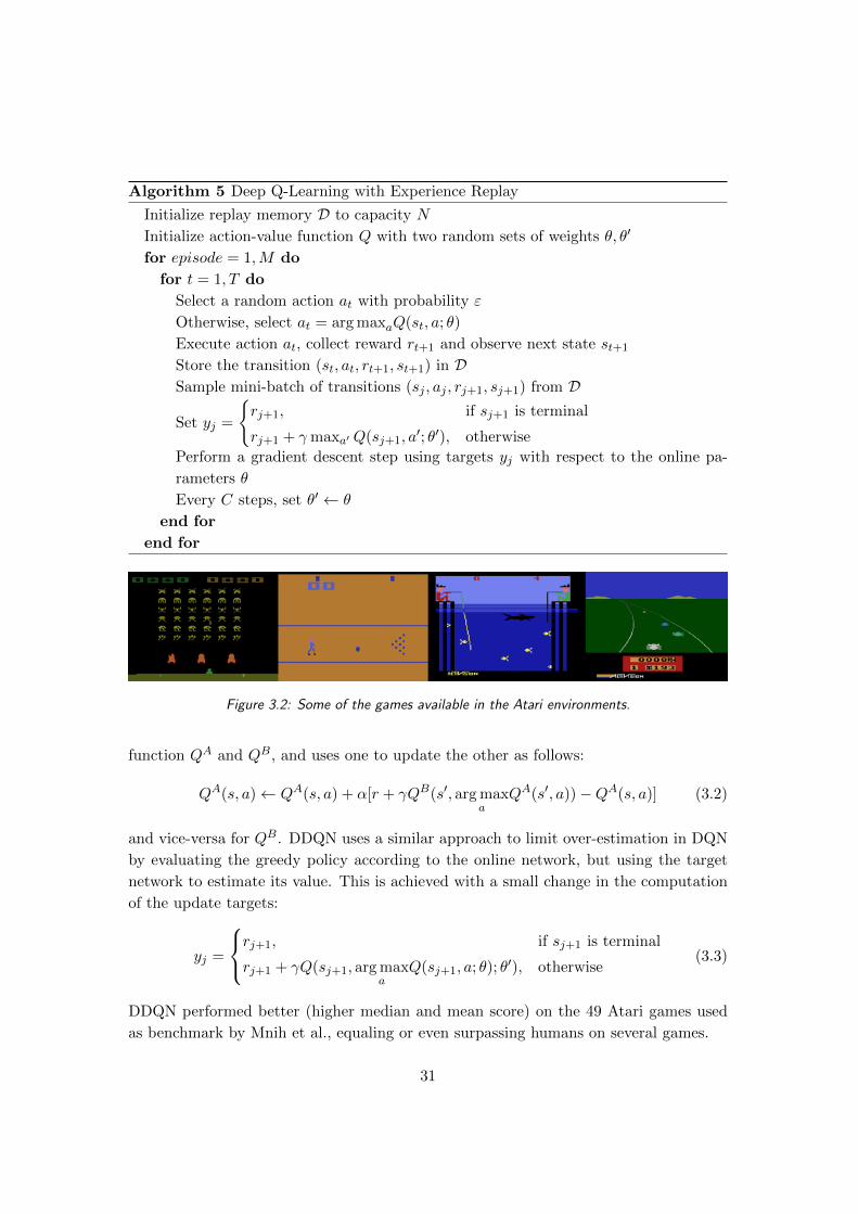
Algorithm 5 Deep Q-Learning with Experience Replay
Initialize replay memory D to capacity N
Initialize action-value function Q with two random sets of weights θ, θ�
for episode = 1,M do
for t = 1, T do
Select a random action at with probability ε
Otherwise, select at = argmaxaQ(st, a; θ)
Execute action at, collect reward rt+1 and observe next state st+1
Store the transition (st, at, rt+1, st+1) in DSample mini-batch of transitions (sj , aj , rj+1, sj+1) from D
Set yj =
�rj+1, if sj+1 is terminal
rj+1 + γmaxa� Q(sj+1, a�; θ�), otherwise
Perform a gradient descent step using targets yj with respect to the online pa-
rameters θ
Every C steps, set θ� ← θ
end for
end for
Figure 3.2: Some of the games available in the Atari environments.
function QA and QB, and uses one to update the other as follows:
QA(s, a) ← QA(s, a) + α[r + γQB(s�, argmaxa
QA(s�, a))−QA(s, a)] (3.2)
and vice-versa for QB. DDQN uses a similar approach to limit over-estimation in DQN
by evaluating the greedy policy according to the online network, but using the target
network to estimate its value. This is achieved with a small change in the computation
of the update targets:
yj =
rj+1, if sj+1 is terminal
rj+1 + γQ(sj+1, argmaxa
Q(sj+1, a; θ); θ�), otherwise
(3.3)
DDQN performed better (higher median and mean score) on the 49 Atari games used
as benchmark by Mnih et al., equaling or even surpassing humans on several games.
31
Schaul et al. (2016) [38] developed the concept of prioritized experience replay, which
replaced DQN’s uniform sampling strategy from the replay memory with a sampling
strategy weighted by the TD errors committed by the network. This improved the
performance of both DQN and DDQN.
Wang et al. (2016) [45] introduced a slightly different end-to-end dueling architecture,
composed of two different deep estimators: one for the state-value function V and one
for the advantage function A : S ×A → R defined as:
Aπ(s, a) = Qπ(s, a)− V π(s) (3.4)
In this approach, the two networks share the same convolutional layers but use two
separate dense layers. The two streams are then combined to estimate the optimal
action-value function as2:
Qπ(s, a) = V π(s) + (Aπ(s, a)−maxa�
Aπ(s, a�)) (3.5)
Several other extensions of the DQN algorithm have been proposed in recent years.
Among these, we cite Osband et al. (2016) [35] who proposed a better exploration
strategy based on Thompson sampling, to select an exploration policy based on the
probability that it is the optimal policy; He et al. (2017) [21] added a constrained
optimization approach called optimality tightening to propagate the reward faster during
updates and improve accuracy and convergence; Anschel et al. (2017) [2] improved the
variance and instability of DQN by averaging previous Q estimates; Munos et al. (2016)
[33] and Harutyunyan et al. (2016) [17] proposed to incorporate on-policy samples to
the Q-learning target and seamlessly switch between off-policy and on-policy samples,
which again resulted in faster reward propagation and convergence.
3.2 Other Approaches
In this section we present some approaches proposed in DRL literature as alternative to
value-based DRL, characterized by unconventional architectures (e.g. memory modules
in Section 3.2.1) or designed for a specific environment (e.g. the game of Go in Section
3.2.2).
3.2.1 Memory Architectures
Graves et al. (2016) [16] proposed Differentiable Neural Computer (DNC), an architec-
ture in which an ANN has access to an external memory structure, and learns to read
2In the original paper, the authors explicitly indicate the dependence of the estimates on different
parameters (e.g. V π(s, a;φ,α) where φ is the set of parameters of the convolutional layers and α of the
dense layers). For simplicity in the notation, here we report the estimates computed by the network
with the same notation as the estimated functions (i.e. the network which approximates V π is indicated
as V π, and so on...).
32

Figure 3.3: Architecture of NEC (image taken from [36]).
and write data by gradient descent in a goal-oriented manner. This approach outper-
formed normal ANNs and DNC’s precursor Neural Turing Machine [15] on a variety of
query-answering and natural language processing tasks, and was used to solve a simple
moving block puzzle with a form of reinforcement learning in which a sequence of in-
structions describing a goal is coupled to a reward function that evaluates whether the
goal is satisfied (a set-up that resembles an animal training protocol with a symbolic
task cue).
Pritzel et al. (2017) [36] extended the concept of differentiable memory to DQN
with Neural Episodic Control (NEC). In this approach, the DRL agent consists of three
components: a CNN that processes pixel images, a set of memory modules (one per
action), and a dense ANN that converts read-outs from the action memories into action-
values. The memory modules, called differentiable neural dictionaries (DNDs), are
memory structures that resemble the dictionary data type found in computer programs.
DNDs are used in NEC to associate the state embeddings computed by the CNN to
a corresponding Q estimate, for each visited state: a read-out for a key consists in
a weighted sum of the values in the DND, with weights given by normalized kernels
between the lookup key and the corresponding key in memory (see Figure 3.3). DNDs
are populated automatically by the algorithm without learning what to write, which
greatly speeds up the training time with respect to DNC.
NEC outperformed every previous DRL approach on the Atari games, by achieving
better results using less training samples.
3.2.2 AlphaGo
Traditional board games like chess, checkers, Othello and Go are classical test benches
for artificial intelligence. Since the set of rules that characterizes this type of games is
fairly simple to represent in a program, the difficulty in solving these environments stems
from the dimensionality of the state space. Among the cited games, Go was one of the
last board games in which an algorithm had never beaten top human players, because its
33

Figure 3.4: Neural network training pipeline of AlphaGo (image taken from [39]).
characteristic 19×19 board, which allows for approximately 250150 sequences of moves3,
was too complex for exhaustive search methods.
Silver et al. (2016) [39] introduced AlphaGo, a computer program based on DRL
which won 5 games to 0 against the European Go champion in October 2015; soon
after that, AlphaGo defeated 18-time world champion Lee Sedol 4 games to 1 in March
2016, and world champion Ke Jie 3 to 0 in May 2017. After these results, Google
DeepMind (the company behind AlphaGo) decided to retire the program from official
competitions and released a dataset containing 50 self-play games [18]. AlphaGo is
a complex architecture that combines deep CNNs, reinforcement learning, and Monte
Carlo Tree Search (MCTS) [6, 13]. The process is divided in two phases: a neural
network training pipeline and MCTS. In the training pipeline, four different networks
are trained: a supervised learning (SL) policy network trained to predict human moves;
a fast policy network to rapidly sample actions during MC rollouts; a reinforcement
learning policy network that improves the SL network by optimizing the final outcome
of games of self-play; a value network that predicts the winner of games (see Figure 3.4).
Finally, the policy and value networks are combined in an MCTS algorithm that selects
actions with a lookahead search, by building a partial search tree using the estimates
computed with each network.
3Number of legal moves per position elevated to the length of the game.
34

Figure 3.5: The asynchronous architecture of A3C.
3.2.3 Asynchronous Advantage Actor-Critic
Actor-critic algorithms [41] are RL methods that have a separate memory structure to
explicitly represent the policy independent of the value function. The policy structure is
known as the actor, because it is used to select actions, and the estimated value function
is known as the critic, because it criticizes the actions made by the actor. Learning is
always on-policy, as the critic must learn about and critique whatever policy is currently
being followed by the actor. The critique usually takes the form of a TD error which is
used to drive learning in both the actor and the critic, evaluated as:
δt = rt+1 + γV (st+1)− V (st) (3.6)
Mnih et al. (2016) [31] presented a deep variation of the actor-critic algorithm, called
Asynchronous Advantage Actor-Critic (A3C). In this approach, different instances of
actor-critic pairs are run in parallel (Figure 3.5) to obtain a lower-variance estimate of the
value function, without the need of a replay memory to stabilize training. Each worker
consists in a deep CNN with a unique convolutional section and two separate dense
35

networks on top, one for the value function and one for the policy. This asynchronous
methodology was applied to other classical RL algorithms in the same paper; we only
report the actor-critic variant as it was the best performing, with notably shorter training
times than DQN and its variations, but a similar cumulative reward on the Atari games.
3.3 Related Work
Lange and Riedmiller (2010) [27] proposed the Deep Fitted Q-iteration (DFQ) algorithm,
a batch RL method that used deep dense autoencoders to extract a state representation
from pixel images. In this algorithm, a training set of (s, a, r, s�) transitions is collectedwith a random exploration strategy, where s, s� are pixel images of two consecutive
states. The samples are then used to train a dense autoencoder with two neurons in
the innermost layer, which in turn is used to encode all states in the training set. This
encoded dataset is then passed as input to FQI, which produces an estimate for the Q
function using a kernel based approximator. A new policy is then computed from the
estimated Q and the encoder, and the process is repeated starting with the new policy
until the obtained Q is considered satisfactory. The authors applied DFQ to a simple
Gridworld environment with fixed size and goal state, and were able to outperform other
image-based feature extraction methods (like Principal Components Analysis [47]) with
a good sample efficiency.
36

Chapter 4
Deep Feature Extraction for
Sample-Efficient Reinforcement
Learning
As central contribution of this thesis, we propose a DRL algorithm that combines the
feature extraction capabilities of unsupervised deep CNNs with the fast and powerful
batch RL approach of FQI. Given a control problem with high-dimensional states and
a mono-dimensional discrete action space, we use a deep convolutional autoencoder to
map the original state space to a compressed feature space that accounts for information
on the states and the nominal dynamics of the environment (i.e. those changes not
directly influenced by the agent). We reduce the representation further by applying the
Recursive Feature Selection (RFS) algorithm to the extracted state features, and this
minimal state space is then used to run the FQI algorithm. We repeat this procedure
iteratively in a semi-batch approach to bootstrap the algorithm, starting from a fully
random exploration of the environment.
In this chapter we give a formal description of the method and its core components,
whereas technical details of implementation will be discussed in the next chapter.
4.1 Motivation
The state-of-the-art DRL methods listed in the previous chapter are able to outperform
classic RL algorithms in a wide variety of problems, and in some cases are the only possi-
ble way of dealing with high-dimensional control settings like the Atari games. However,
the approaches cited above tend to be grossly sample-inefficient, requiring tens of mil-
lions of samples collected online to reach optimal performance. Several publications
successfully deal with this aspect, but nonetheless leave room for improvement (lower-

ing at most by one order of magnitude the number of samples required). The method
introduced by Lange and Riedmiller (2010) [27] is similar to ours, but their dense archi-
tecture predates the more modern convolutional approaches in image processing and is
less suited than our AE for complex tasks.
The method that we propose tries to improve both aspects of information content
of the compressed feature space and sample efficiency. We extract general features from
the environments in an unsupervised fashion, which forgoes the task-oriented represen-
tation of the current state-of-the-art methods in favor of a description that relates more
closely to the original information content of the states; because of the generality of this
description, the compressed state space can be used with a variety of RL algorithms in
their default setting (like we show with FQI), without having to adapt the deep archi-
tecture to solve the problem end-to-end like in deep Q-learning. Moreover, since deep
features can be difficult to interpret in an abstract way, and in general there is no assur-
ance against redundancy in the representation, we use a feature selection technique on
the extracted space in order to really minimize the description while retaining all infor-
mation required for control. This additional step does not have a substantial impact on
the learning phase, nor on the learned policies (since we do not extract features aimed at
controlling, there is no direct correlation between features and performance, in general),
but by providing an essential representation of the states it allows the feature extraction
method to be stripped of all the useless parameters, resulting in reduced computational
requirements during the control phase (an important aspect in some high-frequency se-
quential decision making problems). Finally, our sample-efficient methodology allows
our agent to learn non-trivial policies using up to two orders of magnitude less samples
than the state-of-the-art approaches, which may be important in those environments
where online sample collection is difficult or expensive.
4.2 Algorithm Description
The general structure of this algorithm is typical of DRL settings: we use a deep ANN
to extract a representation of an environment, and then use that representation to
control an agent with standard RL algorithms. We also add an additional step after the
deep feature extraction to further reduce the representation down to the essential bits
of information required to solve the problem, by using the Recursive Feature Selection
(RFS) [8] algorithm.
We focus exclusively on environments with a discrete and mono-dimensional action
space A = {0, 1, ..., a}, where actions are assigned a unique integer identifier starting
from 0 with no particular order. We also assume to be operating in a three dimensional
state space (channels × height × width) for consistency with the experimental setting
on which we tested the algorithm (with pixel-level state spaces), although in general the
algorithm requires no such assumption and could be easily adapted to higher or lower
38

Figure 4.1: Composition of the three main modules of the algorithm to produce the end-to-end
function Q : S×A → R. Pixel-level states are transformed by the encoder into the 1D feature space
S, which in turn is filtered by RFS into space S. The final representation is used to train FQI, which
outputs an action-value function Q on S × A. The same preprocessing pipeline is then required to
use Q, and the full composition of the three modules effectively consists in an action-value function
on the original state-action space S ×A.
dimensional settings.
The algorithm uses a modular architecture with three different components that are
combined after training to produce an approximator of the action-value function. The
main components of the algorithm are:
1. a deep convolutional autoencoder that we use to extract a representation of the
environment; the purpose of the AE is to map the original, pixel-level state space
S of the environment into a strongly compressed feature space S, that contains
information on both the states and part of the transition model of the environment;
2. the Recursive Feature Selection technique to further reduce the state representa-
tion S and keep only the truly informative features extracted by the AE, effectively
mapping the extracted feature space to a subspace S.
3. the Fitted Q-Iteration learning algorithm to produce an estimator for the action-
value function, with S as domain.
The full procedure consists in alternating a training step and an evaluation step, until
the desired performance is reached.
A training step of the algorithm takes as input a training set T S of four-tuples
(s ∈ S, a ∈ A, r ∈ R, s� ∈ S) to produce an approximation of the action-value function,
and consists in sequentially training the three components from scratch to obtain the
following transformations, respectively:
39

• ENC : S → S, from the pixel representation to a compressed feature space;
• RFS : S → S, from the compressed feature space to a minimal subspace with the
most informative features for control purposes;
• Q : S ×A → R, an approximation of the optimal action-value function on S.
After training, we simply combine the three functions (see Figure 4.1) to obtain the full
action-value function Q : S ×A → R as follows:
Q(s, a) = Q(RFS(ENC(s)), a) (4.1)
To collect the training set T S, we define a greedy policy π based on the current
approximation of Q as:
π(s) = argmaxa
Q(s, a) (4.2)
and we use an ε-greedy policy πε based on π (cf. Section 2.2.1) to collect T S. We
initialize the ε-greedy policy as fully random (which means that we do not need an
approximation of Q for the first step), and we decrease ε after each step down to a
fixed minimum positive value εmin. This results in a sufficiently high exploration at the
beginning of the procedure, but increasingly exploits the learned knowledge to improve
the quality of the collected samples after each training step, as the agent learns to reach
states with a higher value. The lower positive bound on ε is kept to minimize overfitting
and allow the agent to explore potentially better states even in the later steps of the
algorithm. A similar approach, called ε-annealing, was used by Mnih et al. [32] for
the online updates in DQN. Each training step is followed by an evaluation phase to
determine the quality of the learned policy and eventually stop the procedure when the
performance is deemed satisfactory. A general description of the process is reported in
Algorithm 6, and details on the training phases and evaluation step are given in the
following sections.
Note that in general the semi-batch approach, which starts from a training set col-
lected under a fully random policy and sequentially collects new datasets as performance
improves, is not strictly necessary. It is also possible to run a single training step in pure
batch mode, using a dataset collected under an expert policy (albeit with some degree
of exploration required by FQI) to produce an approximation of the optimal Q function
in one step. This allows to exploit the sample efficiency of the algorithm in situations
where, for instance, collecting expert samples is difficult.
4.3 Extraction of State Features
The AE used in our approach consists of two main components, namely an encoder and
a decoder (cf. Section 2.1.4). To the end of explicitly representing the encoding purpose
40

Algorithm 6 Fitted Q-Iteration with Deep State Features
Given:
εmin ∈ (0, 1);
ϕ : [εmin, 1] → [εmin, 1) s.t. ϕ(x) < x, ∀x ∈ (εmin, 1] and ϕ(εmin) = εmin
Initialize the encoder ENC : S → S arbitrarily
Initialize the decoder DEC : S → S arbitrarily
Initialize Q arbitrarily
Define π(s) = argmaxa
Q(s, a)
Initialize an ε-greedy policy πε based on π with ε = 1
repeat
Collect a set T S of four-tuples (s ∈ S, a ∈ A, r ∈ R, s� ∈ S) using πεTrain the composition DEC ◦ ENC : S → S using the state elements (s ∈ S) of
T S as input and target
Build a set T SENC of four-tuples (s ∈ S, a ∈ A, r ∈ R, s� ∈ S) by applying the
encoder to the first and last elements of each four-tuple in T S s.t. s = ENC(s)
Call the RFS feature selection algorithm on T SENC to obtain a space reduction
RFS : S → S
Build a set T SRFS of four-tuples (s ∈ S, a ∈ A, r ∈ R, s� ∈ S) by applying RFS to
the first and last elements of each four-tuple in T SENC s.t. s = RFS(s)
Call FQI on T SRFS to produce Q : S ×A → RCombine Q, RFS and ENC to produce Q : S ×A → R:
Q(s, a) = Q(RFS(ENC(s)), a)
Set ε ← ϕ(ε)
Evaluate π
until stopping condition on evaluation performance is met
Return Q
41

Figure 4.2: Schematic view of the AE.
of the AE, we keep a separate notation of the two modules; we therefore refer to two
different CNNs, namely ENC : S → S to map the original state space to the compressed
representation S, and DEC : S → S to perform the inverse transformation. The full AE
is the composition of the two networks AE : DEC ◦ ENC : S → S (Figure 4.2). Note
that the composition is differentiable end-to-end, and basically consists in plugging the
last layer of the encoder as input to the decoder. Both components are convolutional
neural networks specifically structured to reduce the representation down to an arbitrary
number of features in the new space. We train the AE to reconstruct its input in an
unsupervised fashion, using a dataset T S of four-tuples (s ∈ S, a ∈ A, r ∈ R, s� ∈ S)
collected with the ε-greedy policy and taking the first element (s ∈ S) of each sample as
input and target. The output of this phase is the trained encoder ENC : S → S, which
takes as input the three-dimensional states of the environment and produces a one-
dimensional feature vector representing a high-level abstraction of the state space. We
refer to S as a representation of both the state and the nominal environment dynamics
because we allow for the original state space S to contain both such types of information,
accounting for changes in the environment that are not directly (or even indirectly)
caused by the user. An example of this is the MsPacman environment in the Atari
suite, implementation of the popular arcade game, in which the ghosts are able to
move autonomously, not necessarily influenced by the player; in such a setting, the
environment presents non-trivial nominal dynamics that must be taken into account
in the extracted representation (Figure 4.3). Details on how we accomplish this are
provided in the following chapter, when dealing with the specific implementation of our
experimental setting.
42

Figure 4.3: Example of non-trivial nominal dynamics in the MsPacman environment, with the ghosts
moving autonomously across the four consecutive observations.
4.4 Recursive Feature Selection
The Recursive Feature Selection (RFS) algorithm is a dimensionality reduction technique
for control problems proposed by Castelletti et al. (2011) [8]. The algorithm identifies
which state and action features (i.e. elements of the state and action vector spaces)
are most relevant for control purposes, reducing the dimensionality of both spaces by
removing the less important features. The core of the algorithm consists in recursively
selecting the features that best explain the dynamics (i.e. the transition model) of the
features already selected, starting from the subset of features needed to explain the
reward function, using the Iterative Feature Selection (IFS) [12] algorithm to recursively
build a dependency tree of features.
Algorithm 7 Recursive Feature Selection (RFS)
Given: a dataset D = �s ∈ S, a ∈ A, s� ∈ S�; a target feature F i0 from the set of
features of S ∪A; a set F isel of previously selected features
F iF0
← IFS(D, F i0)
F inew ← F i
F0\ F i
sel
for all F i+1j ∈ F i
new do
F iF0
← F iF0
∪RFS(D, F i+1j ,F i
sel ∪ F iF0)
end for
return F iF0
The main procedure (summarized in Algorithm 7) takes as input a dataset D of
observed transitions from an environment, the values of a target feature F i0 in D, and
a set F isel of previously selected features. The dataset and target feature are given as
input to IFS, which returns a subset of features F iF0
that best explain the dynamics of
F i0. RFS is then recursively called on each feature in the set F i
new = F iF0
\ F isel of new
features selected by IFS. At the first step, the algorithm is usually run to identify the
43

most important features to explain the reward R by setting F 00 = R and F0
sel = ∅, sothat the final output of the procedure will be a set of features that describe the dynamics
of the reward and of the environment itself (a simple example of RFS is given in Figure
4.4).
The IFS procedure called at each step of RFS is a feature selection technique based
on a feature ranking algorithm, but in general can be replaced by any feature selection
method that is able to account for nonlinear dependencies and redundancy between
features (as real-world control problems are usually characterized by nonlinear dynamics
models with multiple coupled features). Here we use IFS for coherence with the paper by
Castelletti et al., and because it is a computationally efficient feature selection algorithm
that works well with our semi-batch approach. IFS takes as input a datasetD of observed
(s, a, r, s�) transitions from the environment and the values of a target feature F0 in D.
The algorithm starts by globally ranking the features of the state space according to a
statistical level of significance provided by a feature ranking method FR, which takes
as input the dataset and the target feature; the most significant feature according to
the ranking, F ∗, is added to the set of selected features Fsel. A supervised model f is
then trained to approximate the target feature F0, taking Fsel as input. The algorithm
then proceeds by repeating the ranking process using as new target feature for FR
the residual feature F0 = F0 − f(Fsel) (the difference between the target value and
the approximation computed by f for each sample in D). The procedure continues to
perform these operations until either the best variable in the feature ranking is already
in Fsel, or the accuracy of the model built upon Fsel does not improve. The accuracy
of the model is computed with the coefficient of determination R2 between the values
of the target feature F0 and the values Fpred = f(Fsel) predicted by the model:
R2(F0, Fpred) = 1−
�k
(f0,k − fpred,k)2
�k
(f0,k − 1|D|
|D|�i=1
f0,i)
(4.3)
The full IFS procedure is summarized in Algorithm 8.
To the extent of our algorithm, we run the RFS procedure on a dataset T SENC of
four-tuples (s ∈ S, a ∈ A, r ∈ R, s� ∈ S) built by applying the transformation ENC to
the first and last elements of each four-tuple in T S. We run the algorithm on all the
state and action features but, since we assume to be working in a mono-dimensional
action space, we force the action feature to always be part of the representation, so that
the procedure is effectively working only on S.
At the end of the procedure, we define a simple filtering operation RFS : S → S
that consists in keeping only the features of S that have been selected by the algorithm.
The output of the training phase is this transformation.
44

Figure 4.4: In this simple example we show the output of RFS in a simple Gridworld environment
with two state features, x and y, to represent the agent’s position and two action features, ax and ayvalued in {−1, 0, 1}, to control the corresponding state features and move the agent on the discrete
grid (the movement is the sum of the two effects). We use a setting with null reward everywhere
except in the four goal states (green) which yield a positive reward, and a wall that cancels the effect
of action ax if the agent tries to move through it. To the right we see the dependency tree produced
by RFS, which in this case selects both state features and both action features. Intuitively, the reward
is explained exclusively by the state feature x and the action that controls it, ax, because the agent
gets a positive reward in each of the four cells to the far right, independently of its y coordinate,
whenever it reaches one. At the same time, feature x is explained by its value and by the action
feature ax (because the next value of x is a function of both, namely x� = x + ax), but also by
feature y, because given the x coordinate of the agent and a direction along x we still have to know
whether the agent is next to the wall in order to compute the following value of x. Finally, feature
y is explained by itself and its associated action, without restrictions given by the wall.
45

Algorithm 8 Iterative Feature Selection (IFS)
Given: a dataset D = �s ∈ S, a ∈ A, s� ∈ S�; a target feature F0 from the set of
features of S ∪A
Initialize: Fsel ← ∅, F0 ← F0, R2old ← 0
repeat
F ∗ ← argmaxF FR(D, F0, F )
if F ∗ ∈ Fsel then
return Fsel
end if
Fsel ← Fsel ∪ F ∗
Build a model f : Fsel → F0 using DFpred = f(Fsel)
F0 ← F0 − Fpred
ΔR2 ← R2(D, F0, Fpred)−R2old
R2old ← R2(D, F0, Fpred)
until ΔR2 < �
return Fsel
4.5 Fitted Q-Iteration
The last component of our training pipeline is the Fitted Q-Iteration algorithm (cf.
Section 2.2.7). We provide as input to the procedure a new training set T SRFS of four-
tuples (s ∈ S, a ∈ A, r ∈ R, s� ∈ S), obtained by applying the RFS transformation to
the first and last elements of each four-tuple in T SENC . We train the model to output a
multi-dimensional estimate of the action-value function on R|A|, with one value for each
action that the agent can take in the environment, and we restrict the output to a single
value on R using the action identifier as index (e.g. Q(s, 0) will return the first dimension
of the model’s output, corresponding to the value of action 0 in state s). The output of
this training phase is the transformation Q : S × A → R, which is then combined with
ENC and RFS as per Equation (4.1) to produce the approximation of Q. This phase
also concludes the training step.
46

Chapter 5
Technical Details and
Implementation
In this chapter we show the implementation details of the architecture used to perform
experiments. We try to provide a complete description of the parametrization of the
components and of the training procedure, in order to ensure reproducibility of the
experimental results.
5.1 Atari Environments
The Arcade Learning Environment (ALE) [3] is an evaluation platform for RL agents.
ALE offers a programmatic interface to hundreds of game environments for the Atari
2600, a popular home video game console developed in 1977 with more than 500 games
available, and is simply referred to as Atari environments (or games). We use the
implementation of ALE provided by the Gym 0.9.2 package for Python 2.7, developed
by OpenAI and maintained as an open source project. This implementation provides
access to the game state in the form of 3 × 110 × 84 RGB frames, produced at an
internal frame-rate of 60 frames per second (FPS). When an action is executed in the
environment, the simulator repeats the action for four consecutive frames of the game
and then provides another observation, effectively lowering the frame rate from 60 FPS
to 15 FPS and making the effects of actions more evident (Figure 5.1).
We perform a preprocessing operation on the states similar to that performed by
Mnih et al. in DQN [32], in order to include all necessary information about the envi-
ronment and its nominal dynamics in the new state representation. First we convert
each RGB observation to a single-channel grayscale representation in the discrete 8-bit

Figure 5.1: Sampling frames at a frequency of 14 in Breakout.
interval [0, 255] using the ITU-R 601-2 luma transform:
L =299
1000R+
587
1000G+
114
1000B (5.1)
where R, G, B are the 8-bit red, green and blue channels of the image. We then
normalize these values in the [0, 1] interval via max-scaling (i.e. dividing each pixel by
255). Moreover, we define a rounding threshold vround specific to each game and we
round all pixel values above or below the threshold to 1 or 0 respectively, reducing the
images to a 1-bit color space in order to facilitate the training of the AE. We also reduce
the height of the image by two pixels in order to prevent information loss due to a
rounding operation performed by the convolution method used in the AE. Finally, we
concatenate the preprocessed observation to the last three preprocessed frames observed
from the environment, effectively blowing up the state space to a 4 × 108 × 84 vector
space (Figure 5.2). The initial state for an episode is artificially set as a repetition of
the first observation provided by the simulator. This operation is needed to include
all necessary information about the environment’s nominal dynamics in the state space
used for training, so that the AE will be able to extract them in the representation.
Moreover, in order to facilitate comparisons and improve stability, we remain loyal
to the methodology used for DQN and perform the same clipping of the reward signal
in a [−1, 1] interval.
We also add a tweak to the Gym implementation of ALE in order to fix a requirement
of some environments of performing some specific actions in order to start an episode
(e.g. in Breakout it is required that the agent takes action 1 to start the game). We
automatically start each episode by randomly selecting one of the initial actions of the
game and forcing the agent to take that action at the beginning of the episode.
Finally, for those games in which the agent has a lives count, we monitor the num-
ber of remaining lives provided by the simulator in the ale.lives parameter. For those
(s, a, r, s�) transitions in which the agent loses a life, we consider s� as a terminal state,
so that the FQI update will only use the reward rather than the full value.
48

Figure 5.2: Two consecutive states s, s� in Pong, after the preprocessing operation. Each binary
image in a sequence of four is an observation of 108× 84 pixels, and the full 4× 108× 84 tensor is
given as input and target to the AE. Notice that between the two consecutive states there are three
frames in common, with the newest observation appended as last frame in s� and the oldest being
pushed out.
Type Input Output # Filters Filter Stride Activation
Conv. 4× 108× 84 32× 26× 20 32 8× 8 4× 4 ReLU
Conv. 32× 26× 20 64× 12× 9 64 4× 4 2× 2 ReLU
Conv. 64× 12× 9 64× 10× 7 64 3× 3 1× 1 ReLU
Conv. 64× 10× 7 16× 8× 5 16 3× 3 1× 1 ReLU
Flatten 16× 8× 5 640 - - - -
Reshape 640 16× 8× 5 - - - -
Deconv. 16× 8× 5 16× 10× 7 16 3× 3 1× 1 ReLU
Deconv. 16× 10× 7 64× 12× 9 64 3× 3 1× 1 ReLU
Deconv. 64× 12× 9 64× 26× 20 64 4× 4 2× 2 ReLU
Deconv. 64× 26× 20 32× 108× 84 32 8× 8 4× 4 ReLU
Deconv. 32× 108× 84 4× 108× 84 4 1× 1 1× 1 Sigmoid
Table 5.1: Layers of the autoencoder with key parameters.
49

5.2 Autoencoder
We use the autoencoder to extract a high level representation S of the state space
in an unsupervised fashion. We structure the AE to take as input the preprocessed
observations from the environment and predict values on the same vector space. The
first four convolutional layers make up the encoder and perform a 2D convolution with
the valid padding algorithm, such that the input of each layer (in the format channels×height × width) is reduced automatically across the last two dimensions (height and
width) according to the following formula:
outputi = �(inputi − filteri + stridei)/stridei� (5.2)
Since the main purpose of pooling layers is to provide translation invariance to the rep-
resentation of the CNN (meaning that slightly shifted or tilted inputs are considered
the same by the network), here we choose to not use pooling layers in order to preserve
the precious information regarding the position of different elements in the game; this
same approach was adopted in DQN. A final Flatten layer is added at the end of the
encoder to provide a 1D representation of the feature space, which is reversed before the
beginning of the decoder. The decoder consists of deconvolutional layers with symmet-
rical filter sizes, filter numbers, and strides with respect to the encoder. Here the valid
padding algorithm is inversed to expand the representation with this formula:
outputi = �(inputi · stridei) + filteri − stridei� (5.3)
A deconvolutional layer is added at the end to reduce the number of channels back to
the original four, without changing the width and height of the frames (i.e. using unitary
filters and strides). All layers in the AE use the Rectified Linear Unit (ReLU) [34, 26]
nonlinearity as activation function, except for the last layer that uses sigmoids to limit
the activations values in the same [0, 1] interval of the input (Figure 5.3). Details of the
AE layers are summarized in Table 5.1.
We train the AE with the Adam optimization algorithm [25] (see Table 5.2 for details
on the hyperparameters) set to minimize the binary cross entropy loss defined as:
L(y, y) = − 1
N
N�
n=1
[ynlog(yn) + (1− yn)log(1− yn)] (5.4)
where y and y are vectors of N target and predicted observations in the state space.
The dataset used for training is built from the dataset collected for the whole learning
procedure described in Algorithm 6, taking only the first elements of the four-tuples
(s, a, r, s�) ∈ T S (which are used as input and targets). We prevent overfitting of the
training set by monitoring the performance of the AE on a held-out set of validation
samples that amounts to roughly 10% of the training data, and stopping the procedure
when the validation loss does not improve by at least 10−5 for five consecutive training
epochs.
50

Figure 5.3: The ReLU and Sigmoid activation functions for the AE.
Parameter Value
Learning rate 0.001
Batch size 32
Exponential decay rate (β1) 0.9
Exponential decay rate (β2) 0.999
Fuzz factor (ε) 10−8
Table 5.2: Optimization hyperparameters for Adam.
Parameter Value
M (Number of base estimators) 50
K (Number of randomly selected attributes) All available attributes
Scoring method Variance reduction
Max tree depth None
nmin (node) 5
nmin (leaf) 2
Table 5.3: Parameters for Extra-Trees and its base estimators in RFS.
51

Parameter Value
K (for K-fold cross-validation) 3
ξ (significance) 0.95
Table 5.4: Parameters for RFS.
5.3 Tree-based Recursive Feature Selection
We use the RFS algorithm to reduce the state space representation computed by the
AE down to the feature space S. We base both the feature ranking method FR and
the model f , used for computing the descriptiveness of the features, on the supervised
Extra-Trees algorithm (cf. Section 2.3.2).
The feature ranking approach with Extra-Trees is based on the idea of scoring each
input feature by estimating the variance reduction produced anytime that the feature
is selected during the tree building process. The ranking score is computed as the
percentage of variance reduction achieved by each feature over the M trees built by the
algorithm.
At the same time, Extra-Trees is a sufficiently powerful and computationally efficient
supervised learning algorithm to use as f . Note that in general FR and f could be
different algorithms with different parametrizations, but Castelletti et al. use the same
regressor for both tasks (as does the code implementation of RFS and IFS that we used
for experiments), and we therefore complied with this choice. The parametrization of
Extra-Trees for FR and f is reported in Table 5.31 (cf. Section 2.3.2).
We use the R2 metric defined in Equation (4.3) to compute the ability of the selected
features to describe the target, in K-fold cross validation over the training set D. We
compute a confidence interval over the scores of the validation predictions as:
CI =
���� 1
|D|
|D|�
i=1
(R2)2 · ( 1
|D|
|D|�
i=1
(R2))2 (5.5)
and we adapt the stopping condition of RFS by setting � = CI + CIold (where the
suffix old has the same meaning as in Algorithm 8) so that the condition becomes
R2 − CI < R2old − CIold. We also multiply � by a significance factor ξ in order to
control the amount of variance that a feature must explain in order to be added to the
selection: higher values of ξ mean that the selection will yield a smaller subset composed
exclusively of very informative features (even if the overall amount of variance explained
is not necessarily the whole possible amount). The hyperparameters used for RFS are
reported in Table 5.4.
1Note that we use two different values for the minimum number of samples required to split an
internal node or a leaf.
52

Parameter Value
M (Number of base estimators) 100
K (Number of randomly selected attributes) All available attributes
Scoring method Variance reduction
Max tree depth None
nmin (node) 2
nmin (leaf) 1
Table 5.5: Parameters for Extra-Trees and its base estimators in FQI.
5.4 Tree-based Fitted Q-Iteration
We use the FQI algorithm to learn an approximation of the Q function from the com-
pressed and reduced state space extracted by the previous two modules. For consistency
with the feature selection algorithm, we use the Extra-Trees learning method as func-
tion approximator for the action-value function. The model is trained to map the 1D
compressed feature space S to the |A|-dimensional action-value space R|A|, and we use
the action identifiers to select the single output value of our approximated Q function.
The parametrization for Extra-Trees is reported in Table 5.5 (cf. Section 2.3.2).
Since the FQI procedure introduces a small bias to the action-value estimate at
each iteration (due to approximation errors), we implement an early stopping procedure
based on the evaluation of the agent’s performance. Every fixed number of iterations,
we evaluate the performance of an ε-greedy policy (with ε = 0.05) based on the current
partial approximation Qi, by composing all the modules in the pipeline to obtain the full
Q as per Equation (4.1). If the agent’s performance does not improve for five consecutive
evaluations, we stop the training and produce the best performing estimation as output
to the training phase. The performance is evaluated by running the policy for five
episodes and averaging the clipped cumulative return of each evaluation episode.
Finally, we consider a discount factor γ = 0.99 for the MDP in order to give impor-
tance to rewards in a sufficiently large time frame.
5.5 Evaluation
An evaluation step is run after each training step of the full procedure. Similarly to
what we do to evaluate the agent’s performance during the training of FQI, here we use
an ε-greedy policy with ε = 0.05 based on the full Q composition of Equation (4.1).
The reason for using a non-zero exploration rate during evaluation is that ALE provides
a fully deterministic initial state for each episode, and by using a deterministic policy
we would always observe the same trajectories (thus making it impossible to evaluate
the Q-value in those state-action pairs that the agent never explores). Using a non-zero
53
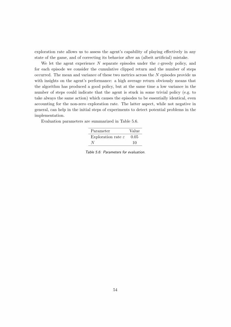
exploration rate allows us to assess the agent’s capability of playing effectively in any
state of the game, and of correcting its behavior after an (albeit artificial) mistake.
We let the agent experience N separate episodes under the ε-greedy policy, and
for each episode we consider the cumulative clipped return and the number of steps
occurred. The mean and variance of these two metrics across the N episodes provide us
with insights on the agent’s performance: a high average return obviously means that
the algorithm has produced a good policy, but at the same time a low variance in the
number of steps could indicate that the agent is stuck in some trivial policy (e.g. to
take always the same action) which causes the episodes to be essentially identical, even
accounting for the non-zero exploration rate. The latter aspect, while not negative in
general, can help in the initial steps of experiments to detect potential problems in the
implementation.
Evaluation parameters are summarized in Table 5.6.
Parameter Value
Exploration rate ε 0.05
N 10
Table 5.6: Parameters for evaluation.
54

Chapter 6
Experimental Results
In this chapter we show experimental results of our algorithm on some Atari games. We
show that the representation of the states learned by our feature extraction pipeline is
suitable for the semi-batch control approach with FQI, and that our agent is able to
learn non-trivial policies with good sample efficiency on different environments.
6.1 Premise
Our approach aims at optimizing sample efficiency, but does not account for the com-
putational complexity of training and evaluating the full pipeline. All three main com-
ponents of the algorithm benefit a great deal from parallel computing, to the point
where the hardware itself is a key component in making the algorithm treatable at all.
We were thus strongly limited in our experimental phase by our access to hardware for
heavy parallel computing, with even costs for renting servers on cloud providers being
prohibitive when considering our runtime. We therefore had to be extremely selective in
what experiments to run, each of which took days at a time, and well balanced between
exploring new possibilities (hyperparameters, network architectures, environments) and
evaluating current configurations. In this chapter we report the best findings across all
our experiments and we try to outline the thought process that led us to favor some
choices over others. The hardware configurations of the three servers that we used for
experiments is reported in Table 6.1.
The code implementation of the algorithm was based on Python 2.7 and its de facto
standard libraries for general machine learning, GPU-based deep learning, and linear
algebra. We trained and used the AE on an Nvidia Tesla K40C GPU, using the Keras
2.0.6 API as interface to the Tensorflow 1.3.0 library for deep learning, whereas the
training and evaluation of Extra-Trees for RFS and FQI were run on CPU using the
Scikit-Learn 0.19.0 library. We used the implementations of FQI and RFS provided in
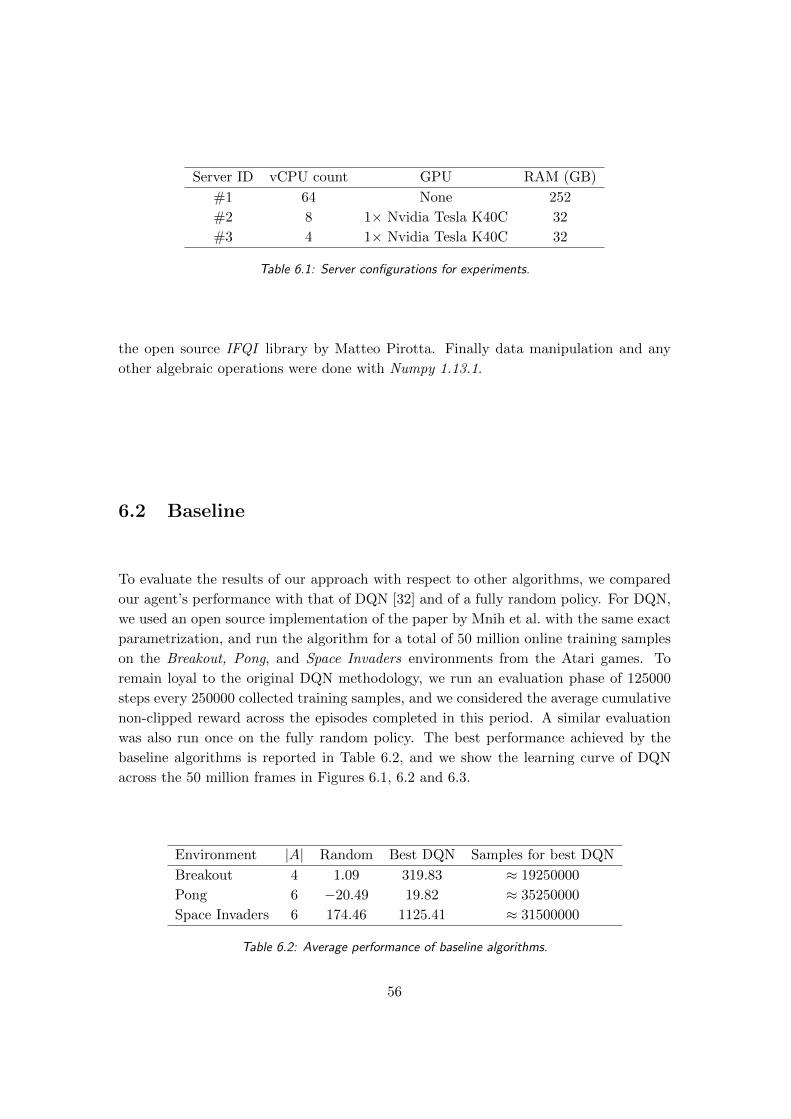
Server ID vCPU count GPU RAM (GB)
#1 64 None 252
#2 8 1× Nvidia Tesla K40C 32
#3 4 1× Nvidia Tesla K40C 32
Table 6.1: Server configurations for experiments.
the open source IFQI library by Matteo Pirotta. Finally data manipulation and any
other algebraic operations were done with Numpy 1.13.1.
6.2 Baseline
To evaluate the results of our approach with respect to other algorithms, we compared
our agent’s performance with that of DQN [32] and of a fully random policy. For DQN,
we used an open source implementation of the paper by Mnih et al. with the same exact
parametrization, and run the algorithm for a total of 50 million online training samples
on the Breakout, Pong, and Space Invaders environments from the Atari games. To
remain loyal to the original DQN methodology, we run an evaluation phase of 125000
steps every 250000 collected training samples, and we considered the average cumulative
non-clipped reward across the episodes completed in this period. A similar evaluation
was also run once on the fully random policy. The best performance achieved by the
baseline algorithms is reported in Table 6.2, and we show the learning curve of DQN
across the 50 million frames in Figures 6.1, 6.2 and 6.3.
Environment |A| Random Best DQN Samples for best DQN
Breakout 4 1.09 319.83 ≈ 19250000
Pong 6 −20.49 19.82 ≈ 35250000
Space Invaders 6 174.46 1125.41 ≈ 31500000
Table 6.2: Average performance of baseline algorithms.
56

Figure 6.1: Average evaluation reward of DQN in Breakout (each point is the average score over
125000 evaluation steps).
Figure 6.2: Average evaluation reward of DQN in Pong (each point is the average score over 125000
evaluation steps).
57

Figure 6.3: Average evaluation reward of DQN in Space Invaders (each point is the average score
over 125000 evaluation steps).
6.3 Autoencoder
Due to the extremely high training and (especially) evaluation times that we encountered
in FQI1, and the almost intractable runtime of RFS2, we had to formally assess the
suitability of the extracted features for control problems before moving on to training the
other components in the pipeline. To do so, we run a series of tests devised to highlight
different aspects of success in the feature extraction. Once a training configuration was
deemed satisfactory, we kept it fixed for all the following experiments.
The most simple test that we run consisted in assessing the reconstruction loss and
accuracy of the AE on a held-out validation set (cf. Section 5.2). We were able to achieve
very high reconstruction accuracy in all environments, with no sensible differences be-
tween training sets collected under different exploration rates. In Table 6.3 we report
validation performance of the AE on datasets of ≈ 50000 samples collected with different
values of ε (see also Figures 6.4, 6.5, and 6.6). In general, the reconstruction of the AE
is better when the training dataset is collected under a high exploration rate. This is
1Slow performance in evaluation is due to the sample-wise forward prediction across the full pipeline
required at each step of evaluation episodes. Specifically, each prediction of the Q function needs a
forward pass of the 4-layer encoder (which requires loading data in the GPU) and a forward pass of
Extra-Trees (which due to an internal inefficiency in Scikit-learn was extremely slow when predicting
on a single sample).2Which can take more than a week to complete, on our most performing server.
58

Environment ε Val. loss Val. accuracy
Breakout
1.0 ≈ 10−5 1.0
0.55 ≈ 10−4 0.9999
0.1 ≈ 10−4 0.9997
Pong
1.0 ≈ 10−4 0.9999
0.55 ≈ 10−4 0.9997
0.1 ≈ 10−4 0.9993
Space Invaders
1.0 ≈ 10−3 0.9987
0.55 ≈ 10−3 0.9985
0.1 ≈ 10−3 0.9978
Table 6.3: Validation performance of our AE on fully random datasets of ≈ 50000 samples.
Figure 6.4: AE reconstruction and feature maps on Breakout. Each pair in the top row shows a
frame of a 4-channel state s given as input to the AE, with its associated reconstructed channel. The
bottom two rows show the relative activation values of the innermost feature maps before the flatten
layer, after encoding s: colors represent a heatmap from black (0) to white (map-wise maximum
activation value). The same applies to Figures 6.5 and 6.6.
59

Figure 6.5: AE reconstruction and feature maps on Pong.
Figure 6.6: AE reconstruction and feature maps on Space Invaders. Note that the lower accuracy
here translates to a poor definition in reconstructing moving elements like the player’s character and
projectiles.
60

Environment ε R2 MSE
Breakout
1.0 0.937 0.0272
0.55 0.854 0.0761
0.1 0.855 0.0748
Pong
1.0 0.945 0.0167
0.55 0.849 0.0334
0.1 0.905 0.0241
Space Invaders
1.0 0.532 0.3895
0.55 0.468 0.5032
0.1 0.457 0.5126
Table 6.4: Results of the S-Q mapping experiment with different exploration rates to collect the
datasets.
intuitively due to the fact that more random policies are less effective and can only reach
a few states, so that the AE has to learn a simpler representation of the environment
(e.g. there is no point in learning to reconstruct the higher layers of the wall in Breakout
if the agent never breaks them). This does not apply to environments like Pong, in
which the agent has no effect on the fixed elements of the game, and for which we see
an almost constant reconstruction accuracy with all exploration rates. Less formally, a
visual inspection of the reconstruction helped us in the early experimental phases and
highlighted how even a small change in accuracy (in the order of 10−3) could result in an
incredibly noisy output. This can be seen in Figure 6.6, where a 99.8% reconstruction
accuracy on Space Invaders means that the AE is not able to reconstruct some small
moving elements of the game.
At the same time, we also inspected the values and behaviors of the features maps
produced by the encoder before flattening, by creating short animations (See Figures
6.4, 6.5, and 6.6) of how the activation values changed in a sequence of about a hundred
states. This confirmed that the extracted features maps contained abstract enough in-
formation (without excessive spatial correlation between the features). We also observed
that in Space Invaders, on average, almost half of the features died. This phenomenon is
a common occurrence in CNNs that use the ReLU activation function (due to the fact
that ReLU has a null gradient for all inputs lower or equal than zero, cf. Figure 5.3), but
we were not able to explain such a high death rate on this particular environment, which
presents a more complicated structure than the other environments that we tested.
In order to truly assess the compatibility of the extracted features with control
problems, we also trained a supervised model to learn the Q approximation produced
by DQN using the extracted features (we call this an S-Q test). We used a training set
composed of tuples (ENC(s) ∈ S, q ∈ R|A|), where s is a state from the environment,
after the preprocessing described in Section 5.1, and q is the |A|-dimensional estimate
61

produced by DQN when it receives s as input. Note that we could use the same input
for both networks, because the preprocessing that we perform on the observations before
feeding a sample to the encoder (cf. Section 5.1) is basically the same that is applied to
the inputs for DQN. To account for the slight different preprocessing, we computed q
before applying the transformations which are unique to our preprocessing, namely the
binarization and cropping. For each environment, we used the best performing DQN
(as per Section 6.2) to produce the targets, and we sampled ≈ 50000 states from the
same dataset on which the AE was trained. To learn the Q approximation, we used
the same Extra-Trees model and hyperparameters that we use for FQI (See Table 5.5),
to ensure that the configuration itself was adequate to describe the nonlinear relations
between the features and the action-value function at convergence of FQI. This was
done by simply fitting the model on the (ENC(s), q) pairs, and evaluating the R2 score
(cf. Definition (4.3)) and Mean Squared Error (MSE) of the predictions on a held-out
validation set of roughly 5% of the training samples. As seen in Figure 6.7, the extracted
features are suitable for describing the Q function learned by DQN with a good degree
of precision, and constitute an adequate base for our whole approach. We were able
to obtain an average R2 score of 0.88, 0.90, and 0.48 on all three tested environments
respectively. Similarly to what we observed for the AE, in Space Invaders we have a
drop in performance probably due to a difficulty in representing all elements in the
environment. For instance, since the AE is not able to properly represent the character
and its projectiles, we can assume that there are no features that describe these elements.
However, these are essential to predict the reward and, consequently, the Q function,
and their absence could explain the bad prediction. We report the results of these tests,
run on datasets collected with different values of ε at different iterations of our full
algorithm, in Table 6.4.
6.4 Recursive Feature Selection
The main purpose of RFS in our learning pipeline is to provide a fast forward propagation
of the AE at control time, by keeping only the AE weights that are essential for the
representation. The runtime of RFS, however, is the longest amongst the three main
components, taking up to a week to complete and extending the runtime of the full
algorithm to a point where it becomes unfeasible. We therefore had to ignore RFS
during most of our experiments, resorting to only running it once per environment
using a dataset collected under a fully random policy and an AE trained on the same
dataset (as if we were running the selection at the first step of the main procedure). At
the same time, we found it appropriate to run another simple feature selection technique
which consisted in only keeping those features with nonzero variance (NZV), in order to
simplify our feature space without losing information. We found that RFS reduced the
representation by up to 60% with respect to NZV on Pong, which indicates that the AE
62

Figure 6.7: Values predicted by the supervised model in the S-Q test vs. real values predicted by
DQN. Note that the |A|-dimensional estimate of the Q function is flattened and treated as a sequence
of |A| independent values in order to plot it.
63

Environment Original NZV RFS Action selected (RFS)
Breakout 640 599 4 No
Pong 640 585 245 Yes
Space Invaders 640 320 640 Yes
Table 6.5: Number of features kept by the two feature selection techniques that we used in our
experiments, run on datasets of 100000 samples collected under a fully random policy.
Environment Score Samples Step ε FQI epoch
Breakout 17 100000 2 of 3 0.55 400
Pong −9 100000 2 of 3 0.55 350
Space Invaders 460 100000 2 of 3 0.55 450
Table 6.6: Best average performance reached by our agent on different environments.
does indeed extract a great deal of redundancy that can be ignored for control purposes.
However, we were not able to replicate this performance on the other two environments.
In Breakout, RFS only selected four state features and did not select the action. On the
other hand, this behavior was inverted on Space Invaders, where the procedure selected
all state and action features (including those with zero variance removed by NZV) at
the first step, when explaining the reward. The reason for this inconsistent behavior
by RFS is probably due to an incompatibility between the RFS procedure itself and
the dynamics of the features extracted by the AE but, as we will show in the following
sections, this does not prevent the agent from learning a good policy using the AE’s
representation. In Figures 6.8 and 6.9, we show the feature dependency trees built by
RFS on Breakout and Pong (we omit the tree from Space Invaders because it is of little
informative value).
6.5 Fitted Q-Iteration
The final part of our experimental methodology consisted in running the full learning
pipeline as described in Algorithm 6, and evaluating the performance of our algorithm
in terms of average reward as we did for DQN and the random policy in Section 6.2. As
we mentioned in the previous section, due to the excessively long computational times
of RFS we chose to remove the module entirely from the pipeline, resorting to simply
keeping those features with nonzero variance across the dataset. At the same time, we
also had to deal with the long runtime for the evaluation of the policy during training of
FQI (necessary for early stopping), due to a general computational complexity of our Q
approximation itself, and to an internal inefficiency in the software library that we used
for Extra-Trees. We tried to address this issue by training FQI for 50 iterations at a
64

Figure 6.8: RFS dependency tree in Breakout. Note how the procedure in this case is not able to
correctly understand the dynamics of the environment and only keeps four state features without
even keeping the action, indicating that in this case the features extracted by the AE are not suitable
for control-oriented selection.
time before evaluating the current policy, for a total of 20 overall evaluations across 1000
training iterations. This resulted in a noisy evaluation performance, but no more noisy
than when we tested the policy at each iteration. We also had to face computational
complexity when deciding how many steps of the main algorithm to run. We decided to
use a custom ϕ function to reduce ε (cf. Section 4.2) dependent on the total number of
steps, so that ε would reach εmin at the last iteration, and at each step would decrease
by a fixed quantity as follows:
ϕ(ε) = ε− 1− εmin
I(6.1)
where I is the total number of iterations (note that the rule only applies if ε is greater
that εmin). We run a comparison of different values of ε at different steps of the pro-
cedure, and we eventually decided to settle for running three iterations (I = 3) with
εmin = 0.1, so that we used the values ε = 1, ε = 0.55 and ε = 0.1 in sequence. This
resulted in a tractable runtime for the full algorithm (however still in the order of days)
and an overall good variety in exploration.
Since the main focus of our work was to minimize the number of training samples, we
empirically tried different sizes for the training sets collected at each step. We started
from a conservative size of 1 million samples, and gradually reduced this amount while
65

Figure 6.9: RFS dependency tree in Pong (showing only topmost 50 nodes).
66

Environment Random Ours DQN Score ratio Sample ratio
Breakout 1 17 319 0.05 0.005
Pong −20 −9 19 0.3 0.002
Space Invaders 174 460 1125 0.4 0.003
Table 6.7: Best average performance of our algorithm compared to the baseline algorithms, and a
relative comparison between our algorithm and DQN. Sample ratio is computed using the number of
samples required by our algorithm and DQN to reach their best performance as reported in Tables
6.2 and 6.6. Note that the score in Pong is shifted to a [0, 42] range to compute the score ratio.
Environment Ours (100k) DQN (100k) Score ratio
Breakout 17 2 8.5
Pong -9 −20 12
Space Invaders 460 145 3.17
Table 6.8: Performance of our algorithm on small datasets compared to DQN’s. The first two
columns show the best score achieved by the algorithms after 100000 training samples. Note that
the score in Pong is shifted to a [0, 42] range to compute the score ratio.
monitoring the agent’s top performance. We were not able to notice a sensible difference
between any dataset size above 50000, so we eventually settled for this amount and kept
it fixed during experiments.
Moving on to the main results of the FQI training, we report the performance of
our algorithm in Tables 6.6, 6.7, 6.8 and 6.9. In Table 6.6, we show the best average
evaluation score achieved by our agent during the main training procedure. We note that
FQI benefits a great deal by a sufficiently high exploration rate, with peak performance
typically reached at ε ≈ 0.5 (this result was often observed during experiments, even
with different configurations for the AE and FQI). Despite being an expected result due
to the fact that FQI needs to learn at once the value of both good and poor states,
unlike online neural algorithms like DQN that can exploit an intrinsic memory of the
architecture to store information about previous samples, this also meant that we only
reached peak performance with our agent at the second main step, with ε = 0.55. We
found that this result was consistent throughout our tests, and we also partly attribute
Environment Ours DQN
Breakout 1.7 · 10−4 1.6 · 10−5
Pong 1.2 · 10−4 1.1 · 10−6
Space Invaders 4.6 · 10−3 3.6 · 10−5
Table 6.9: Sample efficiency of our algorithm compared to DQN’s, computed as best average per-
formance per training sample.
67

to this aspect the inferior performance of our methodology with respect to the state
of the art, because we could never properly exploit the learned knowledge to explore
the environment to the required degree. Our agent could consistently achieve a non-
trivial performance on all environments nonetheless, as reported in Table 6.7, reaching
on average 25% of DQN’s score.
However, despite these poor general results we were able to achieve our main ob-
jective of sample efficiency. Our agent was consistently able to outperform DQN when
considering the amount of samples collected by our procedure to reach its best per-
formance. In Table 6.8, we show how the performance of our algorithm at its best is
on average almost eight times better than DQN’s after collecting the same amount of
samples (roughly 100000). At the same time, even if our best scores amounted to at
best 40% of DQN’s score, we were able to achieve them with as little as 0.2% of the
collected samples (cf. Table 6.7). From this consideration, we explicitly compute the
sample efficiency of the two algorithms by considering the ratio between their best aver-
age score and the number of samples required to achieve it. We show in Table 6.9 that
our agent was able to obtain a higher average reward per training sample, surpassing
DQN’s efficiency by two orders of magnitude.
68

Chapter 7
Conclusions and Future
Developments
In this work we presented a modular deep reinforcement learning procedure with the
objective of improving the sample efficiency of this class of algorithms. The main reason
to explore the potential of our approach is to apply control algorithms to those problem
with a big state space, and from which it is difficult or expensive to collect samples for
learning.
We combined the feature extraction capabilities of unsupervised deep learning and
the control-oriented feature selection of RFS, in order to reduce the pixel-level state
space of Atari games down to a more tractable feature space of essential information
about the environment, from which we then learned a control policy using the batch
reinforcement learning FQI algorithm. Our autoencoder was able to achieve good recon-
struction accuracy on all the environments, and we manged to extract a representation
of the state space which proved to be suitable for approximating the optimal action-
value function. Due to a limit of the computational power that we had available during
the experimental phase, we were not able to explore the capabilities of RFS fully, and
we had to remove it from the pipeline without being able to compare the performance
of our algorithm before and after reducing the feature space. The only experiments that
we were able to run on RFS provided us with mixed information, reducing the state
space as expected on some environments but failing completely on others. The training
of FQI on the feature space resulted in a sub-optimal performance, and highlighted an
intrinsic inefficiency in our semi-batch approach, but we were nonetheless successful in
reaching our objectives.
Our algorithm proved to be less powerful than DQN in learning an optimal control
policy on the environments we tested, as our agent was never able to surpass the scores
of DeepMind’s algorithms. However, we were able to obtain a good sample efficiency,

which allowed our agent to learn good policies using as little as 50000 samples, sur-
passing the performance of DQN by eight times on average when comparing the two
methods using the same amount of samples that our agent required to get to its best
performance. Moreover, we showed that the relative difference in performance between
the two algorithms is smaller than the relative difference in required training samples,
as we were able to achieve on average 25% of DQN’s score using as little as 0.2% of the
samples, thus making our algorithm two orders of magnitude more efficient than DQN.
Our algorithm makes a step towards a more sample-efficient DRL, and to the best
of our knowledge would be a better pick than DQN in settings characterized by a lack
of training samples and a big state space. The sub-optimal performance reached by our
agent only encourages us to explore the possibilities of our algorithm further.
7.1 Future Developments
We extended the work by Lange and Riedmiller (2010) [27] to cover more complex
environments, and we tried to deviate as little as possible from the methodology of Mnih
et al. in DQN in order to facilitate comparison. However, we feel that our research is
far from complete, and in this section we propose some paths on which we would like to
continue.
First of all, in the light of the recently published work by Higgins et al. (2017) [23]
on control-oriented feature extraction using autoencoders, we propose to apply β Vari-
ational Autoencoders (β-VAE) [24, 22] instead of the purely convolutional AE presented
in this work (more similar to the DQN methodology), with the aim of extracting dis-
entangled features that are associated almost one-to-one with specific elements in the
environments. A second approach that we briefly explored during the writing of this
thesis consisted in training the AE in an almost supervised way, using the states of
the environment as input and the following states as output. This would change the
extracted feature space to account for the full dynamics of the environment (rather
than simply the nominal dynamics that we considered by stacking consecutive observa-
tions), which would eventually encode much more appropriate information to the end of
approximating the Q function. On a similar direction, we propose to combine the unsu-
pervised feature extraction with a supervised feature extraction, aimed at representing
some specific information about the environment and its dynamics. When researching
the methodology presented in this thesis, we tried to add to the feature space some
features extracted by a CNN trained to approximate the reward function, but we only
saw a small improvement in performance at the cost of almost doubled runtimes for
RFS and FQI. Another example of this could be the pretraining of the encoder on the
state dynamics, as presented by Anderson et al. (2015) [1]. Moving on to the other
components of our learning pipeline, we would also like to expand the work on RFS and
FQI.
70

As we said in Chapter 6, we were not able to properly explore the capabilities of RFS
due to computational limitations. In order to complete the brief tests that we run for
this work, we propose to directly compare the performance of the full algorithm using
the feature space before and after the selection. This comparison could be the base for
a theoretical analysis of the effect of feature selection on deep features. Moreover, a
systematic analysis of the actual importance of the features in the representation could
lead to better insights on the feature extraction process.
Finally, we think that the batch approach based on FQI could be explored further.
Different models, parameters and features could impact greatly on the performance of
FQI, even if we were not able to highlight the magnitude of this impact in our tests.
Another approach could also change the reinforcement learning component altogether,
by moving to a different algorithm like Q-learning while keeping the extraction and
selection modules unchanged. A technique like experience replay would also probably
help in solving the issue of exploration highlighted in Section 6.5.
71

72

Bibliography
[1] Charles W Anderson, Minwoo Lee, and Daniel L Elliott. Faster reinforcement
learning after pretraining deep networks to predict state dynamics. In International
Joint Conference on Neural Networks (IJCNN), pages 1–7. IEEE, 2015.
[2] Oron Anschel, Nir Baram, and Nahum Shimkin. Averaged-dqn: variance reduction
and stabilization for deep reinforcement learning. In International Conference on
Machine Learning (ICML), pages 176–185, 2017.
[3] Marc G Bellemare, Yavar Naddaf, Joel Veness, and Michael Bowling. The arcade
learning environment: An evaluation platform for general agents. Journal of Arti-
ficial Intelligence Research (JAIR), 47:253–279, 2013.
[4] Dimitri P. Bertsekas and John N. Tsitsiklis. Neuro-dynamic programming: an
overview. In IEEE Conference on Decision and Control, volume 1, pages 560–564.
IEEE, 1995.
[5] Christopher M. Bishop. Pattern recognition and machine learning. Springer, 2006.
[6] Cameron B. Browne, Edward Powley, Daniel Whitehouse, Simon M. Lucas, Peter I.
Cowling, Philipp Rohlfshagen, Stephen Tavener, Diego Perez, Spyridon Samoth-
rakis, and Simon Colton. A survey of monte carlo tree search methods. IEEE
Transactions on Computational Intelligence and AI in games, 4(1):1–43, 2012.
[7] Murray Campbell, A. Joseph Hoane, and Feng-hsiung Hsu. Deep blue. Artificial
Intelligence, 134(1-2):57–83, 2002.
[8] Andrea Castelletti, Stefano Galelli, Marcello Restelli, and Rodolfo Soncini-Sessa.
Tree-based variable selection for dimensionality reduction of large-scale control sys-
tems. In Adaptive Dynamic Programming And Reinforcement Learning (ADPRL),
pages 62–69. IEEE, 2011.
[9] John Duchi, Elad Hazan, and Yoram Singer. Adaptive subgradient methods for
online learning and stochastic optimization. Journal of Machine Learning Research
(JMLR), 12(Jul):2121–2159, 2011.
73

[10] Dumitru Erhan, Yoshua Bengio, Aaron Courville, Pierre-Antoine Manzagol, Pascal
Vincent, and Samy Bengio. Why does unsupervised pre-training help deep learning?
Journal of Machine Learning Research (JMLR), 11(Feb):625–660, 2010.
[11] Damien Ernst, Pierre Geurts, and Louis Wehenkel. Tree-based batch mode rein-
forcement learning. Journal of Machine Learning Research (JMLR), 6(Apr):503–
556, 2005.
[12] S. Galelli and A. Castelletti. Tree-based iterative input variable selection for hy-
drological modeling. Water Resources Research, 49(7):4295–4310, 2013.
[13] Sylvain Gelly, Levente Kocsis, Marc Schoenauer, Michele Sebag, David Silver,
Csaba Szepesvari, and Olivier Teytaud. The grand challenge of computer go: Monte
carlo tree search and extensions. Communications of the ACM, 55(3):106–113, 2012.
[14] Pierre Geurts, Damien Ernst, and Louis Wehenkel. Extremely randomized trees.
Machine Learning, 63(1):3–42, 2006.
[15] Alex Graves, Greg Wayne, and Ivo Danihelka. Neural turing machines. arXiv
preprint arXiv:1410.5401, 2014.
[16] Alex Graves, Greg Wayne, Malcolm Reynolds, Tim Harley, Ivo Danihelka, Ag-
nieszka Grabska-Barwinska, Sergio Gomez Colmenarejo, Edward Grefenstette,
Tiago Ramalho, John Agapiou, AdriA Badia, Karl Moritz Hermann, Yori Zwols,
Georg Ostrovski, Adam Cain, Helen King, Christopher Summerfield, Phil Blun-
som, Koray Kavukcuoglu, and Demis Hassabis. Hybrid computing using a neural
network with dynamic external memory. Nature, 538(7626):471–476, 2016.
[17] A. Harutyunyan, M. G. Bellemare, T. Stepleton, and R. Munos. Q(λ) with off-
policy corrections. In International Conference on Algorithmic Learning Theory,
pages 305–320. Springer, 2016.
[18] D. Hassabis and D. Silver. Alphago’s next move (deepmind.com/blog/alphagos-
next-move/), 2017.
[19] Hado V Hasselt. Double q-learning. In Advances in Neural Information Processing
Systems (NIPS), pages 2613–2621, 2010.
[20] Hado van Hasselt, Arthur Guez, and David Silver. Deep reinforcement learning with
double q-learning. In AAAI Conference on Artificial Intelligence, pages 2094–2100.
AAAI Press, 2016.
[21] F. S. He, Y. Liu, A. G. Schwing, and J. Peng. Learning to play in a day: Faster
deep reinforcement learning by optimality tightening. In International Conference
on Learning Representations (ICLR), 2017.
74

[22] Irina Higgins, Loic Matthey, Arka Pal, Christopher Burgess, Xavier Glorot,
Matthew Botvinick, Shakir Mohamed, and Alexander Lerchner. beta-vae: Learning
basic visual concepts with a constrained variational framework. In International
Conference on Learning Representations (ICLR), 2017.
[23] Irina Higgins, Arka Pal, Andrei Rusu, Loic Matthey, Christopher Burgess, Alexan-
der Pritzel, Matthew Botvinick, Charles Blundell, and Alexander Lerchner. Darla:
improving zero-shot transfer in reinforcement learning. In International Conference
on Machine Learning (ICML), pages 1480–1490, 2017.
[24] D. P. Kingma and M. Welling. Auto-encoding variational bayes. In International
Conference on Learning Representations (ICLR), 2014.
[25] Diederik Kingma and Jimmy Ba. Adam: A method for stochastic optimization.
arXiv preprint arXiv:1412.6980, 2014.
[26] Alex Krizhevsky, Ilya Sutskever, and Geoffrey E Hinton. Imagenet classification
with deep convolutional neural networks. In Advances in Neural Information Pro-
cessing Systems (NIPS), pages 1097–1105, 2012.
[27] Sascha Lange and Martin Riedmiller. Deep auto-encoder neural networks in
reinforcement learning. In International Joint Conference on Neural Networks
(IJCNN), pages 1–8. IEEE, 2010.
[28] Yann LeCun, Yoshua Bengio, and Geoffrey Hinton. Deep learning. Nature,
521(7553):436–444, 2015.
[29] Long-H Lin. Self-improving reactive agents based on reinforcement learning, plan-
ning and teaching. Machine Learning, 8(3/4):69–97, 1992.
[30] Jonathan Masci, Ueli Meier, Dan Ciresan, and Jurgen Schmidhuber. Stacked con-
volutional auto-encoders for hierarchical feature extraction. In International Con-
ference on Artificial Neural Networks (ICANN), pages 52–59, 2011.
[31] Volodymyr Mnih, Adria Puigdomenech Badia, Mehdi Mirza, Alex Graves, Timo-
thy Lillicrap, Tim Harley, David Silver, and Koray Kavukcuoglu. Asynchronous
methods for deep reinforcement learning. In International Conference on Machine
Learning (ICML), pages 1928–1937, 2016.
[32] Volodymyr Mnih, Koray Kavukcuoglu, David Silver, Andrei A. Rusu, Joel Veness,
Marc G. Bellemare, Alex Graves, Martin Riedmiller, Andreas K. Fidjeland, Georg
Ostrovski, Stig Petersen, Charles Beattie, Amir Sadik, Ioannis Antonoglou, Helen
King, Dharshan Kumaran, Dan Wiestra, Shane Legg, and Demis Hassabis. Human-
level control through deep reinforcement learning. Nature, 518(7540):529–33, 2015.
75

[33] R. Munos, T. Stepleton, A. Harutyunyan, and M. Bellemare. Safe and efficient
off-policy reinforcement learning. In Advances in Neural Information Processing
Systems (NIPS), pages 1054–1062, 2016.
[34] Vinod Nair and Geoffrey E Hinton. Rectified linear units improve restricted boltz-
mann machines. In International Conference on Machine Learning (ICML), pages
807–814, 2010.
[35] Ian Osband, Charles Blundell, Alexander Pritzel, and Benjamin Van Roy. Deep
exploration via bootstrapped dqn. In Advances in Neural Information Processing
Systems (NIPS), pages 4026–4034, 2016.
[36] Alexander Pritzel, Benigno Uria, Sriram Srinivasan, Adria Puigdomenech Badia,
Oriol Vinyals, Demis Hassabis, Daan Wierstra, and Charles Blundell. Neural
episodic control. In International Conference on Machine Learning (ICML), 2017.
[37] Gavin A. Rummery and Mahesan Niranjan. On-line Q-learning using connectionist
systems, volume 37. University of Cambridge, Department of Engineering, 1994.
[38] T. Schaul, J. Quan, I. Antonoglou, and D. Silver. Prioritized experience replay. In
International Conference on Learning Representations (ICLR), 2016.
[39] David Silver, Aja Huang, Chris J. Maddison, Arthur Guez, Laurent Sifre, George
van den Driessche, Julian Schrittwieser, Ioannis Antonoglou, Veda Panneershelvam,
Marc Lanctot, Sander Dieleman, Dominik Grewe, John Nham, Nal Kalchbrenner,
Ilya Sutskever, Timothy Lillicrap, Madeleine Leach, Koray Kavukcuoglu, Thore
Graepel, and Demis Hassabis. Mastering the game of go with deep neural networks
and tree search. Nature, 529(7587):484–489, 2016.
[40] Karen Simonyan and Andrew Zisserman. Very deep convolutional networks for
large-scale image recognition. CoRR, abs/1409.1556, 2014.
[41] Richard S. Sutton and Andrew G. Barto. Reinforcement learning: An introduction,
volume 1. MIT press Cambridge, 1998.
[42] Christian Szegedy, Wei Liu, Yangqing Jia, Pierre Sermanet, Scott Reed, Dragomir
Anguelov, Dumitru Erhan, Vincent Vanhoucke, and Andrew Rabinovich. Going
deeper with convolutions. In Computer Vision and Pattern Recognition (CVPR),
pages 1–9. IEEE, 2015.
[43] Gerald Tesauro. Temporal difference learning and td-gammon. Communications of
the ACM, 38(3):58–68, 1995.
76

[44] Aaron van den Oord, Sander Dieleman, Heiga Zen, Karen Simonyan, Oriol Vinyals,
Alex Graves, Nal Kalchbrenner, Andrew Senior, and Koray Kavukcuoglu. Wavenet:
A generative model for raw audio. In 9th ISCA Speech Synthesis Workshop, pages
125–125.
[45] Z. Wang, T. Schaul, M. Hessel, H. van Hasselt, M. Lanctot, and N. de Freitas.
Dueling network architectures for deep reinforcement learning. In International
Conference on Machine Learning (ICML), 2016.
[46] Christopher JCH Watkins and Peter Dayan. Q-learning. Machine Learning, 8(3-
4):279–292, 1992.
[47] Svante Wold, Kim Esbensen, and Paul Geladi. Principal component analysis.
Chemometrics and Intelligent Laboratory Systems, 2(1-3):37–52, 1987.
[48] Yonghui Wu, Mike Schuster, Zhifeng Chen, Quoc V. Le, Mohammad Norouzi, Wolf-
gang Macherey, Maxim Krikun, Yuan Cao, Qin Gao, Klaus Macherey, Jeff Klingner,
Apurva Shah, Melvin Johnson, Xiaobing Liu, Lukasz Kaiser, Stephan Gouws,
Yoshikiyo Kato, Taku Kudo, Hideto Kazawa, Keith Stevens, George Kurian, Nis-
hant Patil, Wei Wang, Cliff Young, Jason Smith, Jason Riesa, Alex Rudnick, Oriol
Vinyals, Greg Corrado, Macduff Hughes, and Jeffrey Dean. Google’s neural ma-
chine translation system: Bridging the gap between human and machine transla-
tion. 2016.
[49] Matthew D. Zeiler. Adadelta: An adaptive learning rate method. arXiv preprint
arXiv:1212.5701, 2012.
[50] Matthew D. Zeiler, Dilip Krishnan, Graham W. Taylor, and Rob Fergus. Decon-
volutional networks. In Computer Vision and Pattern Recognition (CVPR), pages
2528–2535. IEEE, 2010.
77
Related Documents