Deep Feature Extraction for Cymbidium Species Classification ...

Citation: Fu, Q.; Zhang, X.; Zhao, F.;

Ruan, R.; Qian, L.; Li, C. Deep

Feature Extraction for Cymbidium

Species Classification Using

Global–Local CNN. Horticulturae

2022, 8, 470.

https://doi.org/10.3390/

horticulturae8060470

Academic Editor: Jianwei Qin

Received: 12 April 2022

Accepted: 27 April 2022

Published: 25 May 2022

Publisher’s Note: MDPI stays neutral

with regard to jurisdictional claims in

published maps and institutional affil-

iations.

Copyright: © 2022 by the authors.

Licensee MDPI, Basel, Switzerland.

This article is an open access article

distributed under the terms and

conditions of the Creative Commons

Attribution (CC BY) license (https://

creativecommons.org/licenses/by/

4.0/).

horticulturae

Article

Deep Feature Extraction for Cymbidium Species ClassificationUsing Global–Local CNNQiaojuan Fu, Xiaoying Zhang, Fukang Zhao, Ruoxin Ruan, Lihua Qian and Chunnan Li *

Hangzhou Academy of Agricultural Sciences, Hangzhou 311400, China; [email protected] (Q.F.);[email protected] (X.Z.); [email protected] (F.Z.); [email protected] (R.R.); [email protected] (L.Q.)* Correspondence: [email protected]

Abstract: Cymbidium is the most famous and widely distributed type of plant in the Orchidaceaefamily. It has extremely high ornamental and economic value. With the continuous developmentof the Cymbidium industry in recent years, it has become increasingly difficult to classify, identify,develop, and utilize orchids. In this study, a classification model GL-CNN based on a convolutionalneural network was proposed to solve the problem of Cymbidium classification. First, the imageset was expanded by four methods (mirror rotation, salt-and-pepper noise, image sharpening, andrandom angle flip), and then a cascade fusion strategy was used to fit the multiscale features obtainedfrom the two branches. Comparing the performance of GL-CNN with other four classic models(AlexNet, ResNet50, GoogleNet, and VGG16), the results showed that GL-CNN achieves the highestclassification prediction accuracy with a value of 94.13%. This model can effectively detect differentspecies of Cymbidium and provide a reference for the identification of Cymbidium germplasm resources.

Keywords: Cymbidium; classification; global–local CNN; convolutional neural network

1. Introduction

Orchidaceae is one of the largest and most diverse flowering plants and has beenwidespread all around the world [1]. Cymbidium, belonging to the Orchidaceae family,with elegant and upright leaves and fragrant flowers, is the most important and economicflowering genus. It is popular in Asia, especially in China, Japan, Korea, and SoutheastAsia [2]. In China, the Cymbidium has more than a thousand years of history with extremelyhigh cultural and economic value [3]. The flowers of Cymbidium have various colors andshape patterns, which usually leads to confusion when comparing cultivars to assessgenetic resources at the species level [4]. In recent years, with the continuous developmentof the Cymbidium industry, the number of Cymbidium germplasm resources has increasedyear by year, which greatly increases the difficulty of orchid classification, identification,and development. Traditional approaches for the classification of Cymbidium cultivarsare based on morphological traits, which are difficult due to the problems associatedwith morphological variability, growth conditions, overlapping geographical origins, andindividual biases, and most of these cultivars are related [5–7]. It requires professionalsbut offers jugged with subjective. Molecular recognition is the most effective method toidentify the various Cymbidium cultivars [8–10], but often time and cost-consuming, makingit unsuitable for high throughput and rapid classification.

Recently, an emerging field of machine learning, deep learning (DL), known as deepneural networks, has been growing fast and widely used in many fields, such as imageprocessing, content prediction, and text understanding [11]. The main core of the deeplearning algorithm is largely inherited from artificial neural network architecture with manyhidden layers. Deep learning allows computers to process and analyze images and extractimage details similar to the human brain and has been significantly progressed for imagepattern recognition as computer vision algorithms [12]. Convolutional neural network(CNN) is one of the most common methods for visual image classification and has been

Horticulturae 2022, 8, 470. https://doi.org/10.3390/horticulturae8060470 https://www.mdpi.com/journal/horticulturae

Horticulturae 2022, 8, 470 2 of 15

widely adopted by the research community [13]. With the support of powerful graphicsprocessing units (GPU), CNN can be easily used with low-cost normal image data and hugenumbers of datasets, as deep learning often requires large datasets and powerful resourcesfor model training [14]. Inspired by the results of image classification and object detection,many researchers use CNN to identify plant images [15,16]. For instance, CNN has beensuccessfully used to automatically learn discriminative features from leaf images [17] andto detect the diversity in flower images [18]. In addition, the features extracted by CNNcould highly improve classification accuracy and have been suggested to be the optimalcandidate for any visual task [19,20]. CNN has been successfully used to extract features forhyperspectral image (HSI) classification and perform at high accuracy [21]. Hiary et al. [22]conducted a two-step deep learning model that could automatically discover the portionsof flowers and use the feature extracted from this portion to yield a high classificationaccuracy of 97.1% on flowers. Dias et al. [23] also performed feature extraction from afine-tuned CNN model and used these features to establish a support vector machines(SVM) classification model. The model accuracy reached 90% on apple flowers. In addition,a combination of features extracted from pretrained CNN models (AlexNet, ResNet50,and VGG-16) was also used for flower species classification, with a success rate of 80%.These pretrained models have achieved successful results in an ImageNet competition [24].Evidence has shown that combining the feature selection of CNN model and traditionalmachine learning methods, such as SVM and random forest (RF), could yield a high successrate, save massive process time, and reduce computation intensity [25]. However, amongthe available research into CNN technologies, there is limited research into detecting flowerimages of diverse Cymbidium species.

CNN has a powerful ability to capture local features and keep parallel motion un-changed [26]. However, the existing classification methods based on CNN mostly focus onsingle-scale image datasets [27]. Global–local CNN (GL-CNN), a CNN based on multifea-ture fusion, can fuse global and local features. Hao et al. [27] used GL-CNN to classify thegrowth period of Gynura bicolor DC, and the test accuracy of GL-CNN reached 95.63%. Inthis study, we proposed a global–local joint training CNN framework called GL-CNN tosolve the problem of identifying different Cymbidium species instead of using global imageinformation alone. Specific objectives were to: (1) The image set was expanded by fourmethods (mirror rotation, salt-and-pepper noise, image sharpening, and random angleflipping) to improve the model training effect and prevent overfitting. (2) A GL-CNN archi-tecture based on a fusion strategy was proposed to classify 10 different species of Cymbidium.(3) The GL-CNN model was compared with the four classic models (AlexNet, ResNet50,GoogleNet, and VGG16) and the model performance was comprehensively evaluated.

2. Materials and Methods2.1. Cymbidium Species Flower Dataset

In this study, we collected 10 species of Cymbidium, which were C. goeringii, C.longibracteatum, C. faberi, C. sinense, C. hybrids, C. hybridum, C. ensifolium, C. kanran,C. hookerianum, and C. tortisepalum for flower classification. During the flowering period,the flowers of each species were pictured using a high-definition camera (Canon 500D,Tokyo, Japan). There was a total of 3390 pictures. They were divided into two types, asshown in Figure 1. One was an unpicked Cymbidium plant, and the other was a flower ona black background.

Horticulturae 2022, 8, 470 3 of 15Horticulturae 2022, 8, x FOR PEER REVIEW 3 of 15

Figure 1. Examples of pictures of 10 Cymbidium species.

2.2. Data Preprocessing

2.2.1. Two-Scale Image Acquisition

Before model training, Cymbidium images were subjected to two-scale processing to

improve the robustness of the classification model established by the image with different

backgrounds [27]. Figure 2 shows an image sample randomly selected from 10 Cymbidium

species. The red frame represents the second scale image captured. First, set the original

image to a size of 224 × 224 to obtain an image of the first scale. Since the recognition

targets were basically located in the middle of the images, the experiment chose to

intercept a partial image from the center of the first scale image (the height and width of

the partial image were both 0.8 times of the first scale image) as the second scale image.

The size of the second scale image was the same as the first scale image, which was 224 ×

224 [28].

Figure 1. Examples of pictures of 10 Cymbidium species.

2.2. Data Preprocessing2.2.1. Two-Scale Image Acquisition

Before model training, Cymbidium images were subjected to two-scale processing toimprove the robustness of the classification model established by the image with differentbackgrounds [27]. Figure 2 shows an image sample randomly selected from 10 Cymbidiumspecies. The red frame represents the second scale image captured. First, set the originalimage to a size of 224 × 224 to obtain an image of the first scale. Since the recognitiontargets were basically located in the middle of the images, the experiment chose to intercepta partial image from the center of the first scale image (the height and width of the partialimage were both 0.8 times of the first scale image) as the second scale image. The size ofthe second scale image was the same as the first scale image, which was 224 × 224 [28].

Horticulturae 2022, 8, x FOR PEER REVIEW 3 of 15

Figure 1. Examples of pictures of 10 Cymbidium species.

2.2. Data Preprocessing

2.2.1. Two-Scale Image Acquisition

Before model training, Cymbidium images were subjected to two-scale processing to

improve the robustness of the classification model established by the image with different

backgrounds [27]. Figure 2 shows an image sample randomly selected from 10 Cymbidium

species. The red frame represents the second scale image captured. First, set the original

image to a size of 224 × 224 to obtain an image of the first scale. Since the recognition

targets were basically located in the middle of the images, the experiment chose to

intercept a partial image from the center of the first scale image (the height and width of

the partial image were both 0.8 times of the first scale image) as the second scale image.

The size of the second scale image was the same as the first scale image, which was 224 ×

224 [28].

Figure 2. Schematic diagram of two-scale image acquisition.

Horticulturae 2022, 8, 470 4 of 15

2.2.2. Data Set Enhancement

The original data set was divided into training, validation, and test sets at a ratio of8:1:1. Although the diversity of sample species and morphology were considered in theimage collection process, the growth of orchids and the imaging angle were random [26].This experiment mainly chose mirror rotation, sharpening, salt-and-pepper noise, andrandom angle rotation to enhance the image set [29–31]. The total number of samples wasexpanded by four times, and the effects before and after image enhancement are shown inFigure 3.

Horticulturae 2022, 8, x FOR PEER REVIEW 4 of 15

Figure 2. Schematic diagram of two-scale image acquisition.

2.2.2. Data Set Enhancement

The original data set was divided into training, validation, and test sets at a ratio of

8:1:1. Although the diversity of sample species and morphology were considered in the

image collection process, the growth of orchids and the imaging angle were random [26].

This experiment mainly chose mirror rotation, sharpening, salt-and-pepper noise, and

random angle rotation to enhance the image set [29–31]. The total number of samples was

expanded by four times, and the effects before and after image enhancement are shown

in Figure 3.

Figure 3. Examples of the effects before and after image enhancement.

2.3. Global–Local CNN Classification Model

2.3.1. GL-CNN Model Construction

In this part, we proposed a global–local CNN (GL-CNN) network to achieve accurate

classification of different kinds of Cymbidium. The network consists of two types of

features extracted from the trained GL-CNN. The first branch network is the global

feature, denoted as “Gnet.” The second feature is used to capture the local information of

the input image, denoted as “LNet” [27]. The overall network structure is shown in Figure

4. The model input consists of two parts. The original image is input to GNet with a size

of 224 × 224, and the corresponding local images of the same size are input to LNet. There

is a one-to-one correspondence between input images of two scales. This operation

expands the original image information from the data level by expanding the resolution

of the input image in the LNet branch.

This experiment designed different sizes of convolution kernels according to the scale

of the input image in order to enhance the feature extraction ability of the network. As

shown in Figure 4, since GNet extracts global features based on larger-scale images, the

size of the first convolution kernel is set to 11 × 11 to extract edge features. This branch

mainly includes four convolutional layers, three pooling layers, and one fully connected

Figure 3. Examples of the effects before and after image enhancement.

2.3. Global–Local CNN Classification Model2.3.1. GL-CNN Model Construction

In this part, we proposed a global–local CNN (GL-CNN) network to achieve accurateclassification of different kinds of Cymbidium. The network consists of two types of featuresextracted from the trained GL-CNN. The first branch network is the global feature, denotedas “Gnet.” The second feature is used to capture the local information of the input image,denoted as “LNet” [27]. The overall network structure is shown in Figure 4. The modelinput consists of two parts. The original image is input to GNet with a size of 224 × 224,and the corresponding local images of the same size are input to LNet. There is a one-to-onecorrespondence between input images of two scales. This operation expands the originalimage information from the data level by expanding the resolution of the input image inthe LNet branch.

This experiment designed different sizes of convolution kernels according to the scaleof the input image in order to enhance the feature extraction ability of the network. Asshown in Figure 4, since GNet extracts global features based on larger-scale images, thesize of the first convolution kernel is set to 11 × 11 to extract edge features. This branchmainly includes four convolutional layers, three pooling layers, and one fully connectedlayer. Moreover, LNet is a detailed feature extraction branch based on a more fine-grained

Horticulturae 2022, 8, 470 5 of 15

image design, which adds an additional convolutional layer based on GNet to abstract thefeatures [26].

Horticulturae 2022, 8, x FOR PEER REVIEW 5 of 15

layer. Moreover, LNet is a detailed feature extraction branch based on a more fine-grained

image design, which adds an additional convolutional layer based on GNet to abstract the

features [26].

Figure 4. GL-CNN network structure diagram.

2.3.2. Cascade Fusion Strategy

We used the cascade fusion strategy to fit the multiscale features obtained from the

two branches [32]. A feature fusion block was designed to capture features with more

details [31]. With a cascading operation, it can process data layer-by-layer, and it only

merges the two parts of the feature vectors without performing other mathematical

operations. More importantly, the concatenated vector contains all the feature vectors. In

a nutshell, the model can be concerned as an “ensemble of ensembles.”

In order to combine the different features of the global image and the local image, the

“cascade fusion” strategy integrates FC11 and FC12 into the Cas layer through cascade

(Table 1) and sends the Cas feature queue to the FC2 and FC3 layers for further feature

combination and integration. Finally, the prediction probability output is realized through

the SoftMax layer. The main hidden layer parameter settings are shown in Table 1.

Table 1. Details of GL-CNN hidden layer parameters.

Layer Type Size Number of Cores Step Size Output Size Number of Convolutions Number of Neurons

Input - - - - 224 × 224 × 3 - -

Conv11 Convolution 11 × 11 96 4 54 × 54 × 96 (11 × 11 + 1) × 96 54 × 54 × 96

Pool11 Mean-pooling 3 × 3 - 2 26 × 26 × 96 - 26 × 26 × 96

Conv12 Convolution 5 × 5 96 1 26 × 26 × 256 (5 × 5 + 1) × 96 26 × 26 × 96

Pool12 Mean-pooling 3 × 3 - 2 12 × 12 × 96 - 12 × 12 × 96

Conv13 Convolution 3 × 3 192 1 12 × 12 × 384 (3 × 3 + 1) × 192 12 × 12 × 192

Conv14 Convolution 3 × 3 256 1 12 × 12 × 384 (3 × 3 + 1) × 256 12 × 12 × 256

Pool13 Mean-pooling 3 × 3 - 2 5 × 5 × 256 - 5 × 5 × 256

FC11 Fully connected 1 × 1 4096 - 1 × 1 × 4096 (1 × 1 + 1) × 4096 1 × 1 × 2048

Conv21 Convolution 5 × 5 96 3 75 × 75 × 96 (5 × 5 + 1) × 96 75 × 75 × 96

Pool21 Mean-pooling 3 × 3 - 3 25 × 25 × 96 - 25 × 25 × 96

Conv22 Convolution 5 × 5 96 1 25 × 25 × 256 (5 × 5 + 1) × 96 25 × 25 × 96

Pool22 Mean-pooling 3 × 3 - 2 12 × 12 × 96 - 12 × 12 × 96

Conv23 Convolution 3 × 3 192 1 12 × 12 × 384 (3 × 3 + 1) × 192 12 × 12 × 192

Conv24 Convolution 3 × 3 256 1 12 × 12 × 384 (3 × 3 + 1) × 256 12 × 12 × 256

Conv25 Convolution 3 × 3 256 1 12 × 12 × 384 (3 × 3 + 1) × 256 12 × 12 × 256

Pool23 Mean-pooling 3 × 3 - 2 5 × 5 × 256 - 5 × 5 × 256

FC21 Fully connected 1 × 1 4096 - 1 × 1 × 4096 (1 × 1 + 1) × 4096 1 × 1 × 2048

Conv11：

96@11×11

Pool11：

3×3/2

Conv12：

256@5×5

Conv13：

384@3×3

Conv14：

256@3×3

Conv21：

96@5×5

Pool12：

3×3/2

Pool13：

3×3/2

Pool23：

3×3/2Pool21：

3×3/3

Pool22：

3×3/2Conv22：

256@5×5

Conv23：

384@3×3

Conv24：

384@3×3

Conv25：

256@3×3

Input size:

224×224FC11

FC12

Input size:

224×224

LNet

GNet

Cas

FC2 FC3

Figure 4. GL-CNN network structure diagram.

2.3.2. Cascade Fusion Strategy

We used the cascade fusion strategy to fit the multiscale features obtained fromthe two branches [32]. A feature fusion block was designed to capture features withmore details [31]. With a cascading operation, it can process data layer-by-layer, and itonly merges the two parts of the feature vectors without performing other mathematicaloperations. More importantly, the concatenated vector contains all the feature vectors. In anutshell, the model can be concerned as an “ensemble of ensembles.”

In order to combine the different features of the global image and the local image, the“cascade fusion” strategy integrates FC11 and FC12 into the Cas layer through cascade(Table 1) and sends the Cas feature queue to the FC2 and FC3 layers for further featurecombination and integration. Finally, the prediction probability output is realized throughthe SoftMax layer. The main hidden layer parameter settings are shown in Table 1.

Table 1. Details of GL-CNN hidden layer parameters.

Layer Type Size Number of Cores Step Size Output Size Number ofConvolutions

Number ofNeurons

Input - - - - 224 × 224 × 3 - -Conv11 Convolution 11 × 11 96 4 54 × 54 × 96 (11 × 11 + 1) × 96 54 × 54 × 96Pool11 Mean-pooling 3 × 3 - 2 26 × 26 × 96 - 26 × 26 × 96Conv12 Convolution 5 × 5 96 1 26 × 26 × 256 (5 × 5 + 1) × 96 26 × 26 × 96Pool12 Mean-pooling 3 × 3 - 2 12 × 12 × 96 - 12 × 12 × 96Conv13 Convolution 3 × 3 192 1 12 × 12 × 384 (3 × 3 + 1) × 192 12 × 12 × 192Conv14 Convolution 3 × 3 256 1 12 × 12 × 384 (3 × 3 + 1) × 256 12 × 12 × 256Pool13 Mean-pooling 3 × 3 - 2 5 × 5 × 256 - 5 × 5 × 256FC11 Fully connected 1 × 1 4096 - 1 × 1 × 4096 (1 × 1 + 1) × 4096 1 × 1 × 2048

Conv21 Convolution 5 × 5 96 3 75 × 75 × 96 (5 × 5 + 1) × 96 75 × 75 × 96Pool21 Mean-pooling 3 × 3 - 3 25 × 25 × 96 - 25 × 25 × 96Conv22 Convolution 5 × 5 96 1 25 × 25 × 256 (5 × 5 + 1) × 96 25 × 25 × 96Pool22 Mean-pooling 3 × 3 - 2 12 × 12 × 96 - 12 × 12 × 96Conv23 Convolution 3 × 3 192 1 12 × 12 × 384 (3 × 3 + 1) × 192 12 × 12 × 192Conv24 Convolution 3 × 3 256 1 12 × 12 × 384 (3 × 3 + 1) × 256 12 × 12 × 256Conv25 Convolution 3 × 3 256 1 12 × 12 × 384 (3 × 3 + 1) × 256 12 × 12 × 256Pool23 Mean-pooling 3 × 3 - 2 5 × 5 × 256 - 5 × 5 × 256FC21 Fully connected 1 × 1 4096 - 1 × 1 × 4096 (1 × 1 + 1) × 4096 1 × 1 × 2048Cas Cascade - - - 1 × 1 × 8192 - 1 × 1 × 8192FC2 Fully connected 1 × 1 4096 - 1 × 1 × 4096 (1 × 1 + 1) × 4096 1 × 1 × 4096FC3 Fully connected 1 × 1 1000 - 1 × 1 × 1000 (1 × 1 + 1) × 1000 1 × 1 × 1000

Output Output 1 × 1 10 - 1 × 1 × 10 - -

Horticulturae 2022, 8, 470 6 of 15

2.3.3. Model Enhancement

The model uses ReLU6 and dropout to prevent gradient explosion and alleviate poten-tial overfitting problems. End-to-end training is achieved through momentum stochasticgradient descent, and cross-entropy is used as the loss function.

ReLU 6 is an activation function commonly used in deep convolutional neural net-works [27,33]. Relu uses x for linear activation in the region of x > 0, which may cause thevalue after activation to be too large and affect the stability of the model [34]. In order tooffset the linear growth of the ReLU excitation function, the Relu6 function can be used.The ReLU activation function and derivative function are:

ReLU6(x) = min(max(x, 0), 6) ∈ [0, 6] (1)

ReLU6′(x) ={

1, 0 < x < 60, else

∈ {0, 1} (2)

Dropout is used to combat overfitting in artificial neural networks. It can avoidcomplicated mutual adaptation to training data [35]. During the network training process,half of the neurons are usually ignored randomly; that is, the dropout is set to 0.5. Thecross-entropy loss function is used to evaluate the difference between the predicted andactual values of the model [36], which can be expressed as follows:

L =1N ∑i Li = −

1N ∑i ∑M

c=1 yic log(pic) (3)

where M is the number of categories, N is the number of samples, and yic indicates thesymbolic function (0 or 1). If the true category of the sample i is equal to C, take 1, orotherwise take 0. pic indicates the predicted probability of the observation sample with ibelonging to category C.

2.4. Model Training2.4.1. Parameter Settings

Referring to the method of Hao et al. [27], the experiment was performed on a Win-dows 10 64-bit PC equipped with an Intel(R) Xeon(R) CPU @ 3.80 GHz processor, 32 GBRAM, and a GPU of NVIDIA GeForce GTX 3060. The GL-CNN model mentioned in thisarticle is implemented based on the Keras framework. In addition, the maximum numberof iterations epochs is set to 60, the initial learning rate is set to 0.05, and the learning rate isupdated to 1/2 of the original value every 20 epochs. The “SGD+Momentum” strategy isadopted to update the parameters to improve the training speed of the model and avoidfalling into the local optimum at the same time [37].

2.4.2. Contrast Experiment

In order to evaluate the performance of the proposed GL-CNN model in orchid-typeclassification tasks, comparative experiments were carried out with the classic AlexNet,ResNet50, GoogleNet, and VGG16 models. AlexNet is a convolutional neural networkdesigned by Alex Krizhevsky and contains an eight-layer network [38]. The first five layersare convolutional layers, some of the later layers are maximum pooling layers, and the lastthree layers are fully connected layers. It uses a non-saturated ReLU activation functionand shows better training performance than tanh and sigmoid [39]. The Residual NeuralNetwork (ResNet) is an artificial neural network (ANN) that stacks residual blocks ontop of each other to form a network. ResNet-50 is a convolutional neural network with adepth of 50 layers, which can accurately analyze visual images [40]. GoogLeNet is a type ofconvolutional neural network based on the Inception architecture [39]. It utilizes Inceptionmodules, which allow the network to choose between multiple convolutional filter sizesin each block. An Inception network stacks these modules on top of each other, withoccasional max-pooling layers with stride 2 to halve the resolution of the grid. VGG16 is a

Horticulturae 2022, 8, 470 7 of 15

convolutional neural network model proposed by K. Simonyan and A. Zisserman of OxfordUniversity. This model achieves a top-five test accuracy rate of 92.7% in ImageNet [28].

2.4.3. Model Performance Evaluation

Four metrics, namely, precision, recall, F1-score, and accuracy, were used to evaluatethe classification model [27,41], and the formulas are expressed as follows:

Precision =TP

TP + FP(4)

Recall =TP

TP + FN(5)

Accuracy =TP + TN

TP + TN + FP + FN(6)

F1 =2TP

2TP + FP + FN(7)

where true positive (TP) refers to the number of samples whose predicted value and actualvalue are both positive. False positive (FP) refers to the number of samples whose predictedvalue is positive, and the actual value is negative. False negative (FN) means false negative,which refers to the number of samples whose predicted value is negative, and the measuredvalue is positive, correspondingly. True negative (TN) is true negative, which refers to thenumber of samples whose predicted value and actual value are both negative.

3. Results3.1. Data Collection and Preprocessing

In the image samples randomly selected from 10 Cymbidium species shown in Figure 2,it can be observed that the background of the second scale image was smaller, and thedetails of the flower such as veins and textures were more abundant, which was morehelpful to expand the input features and improve the classification accuracy. Four dataenhancement methods, i.e., mirror rotation, sharpening, salt-and-pepper noise, and randomangle rotation, were used to expand the training set by four times to prevent overfitting.

3.2. Model Performance Evaluation

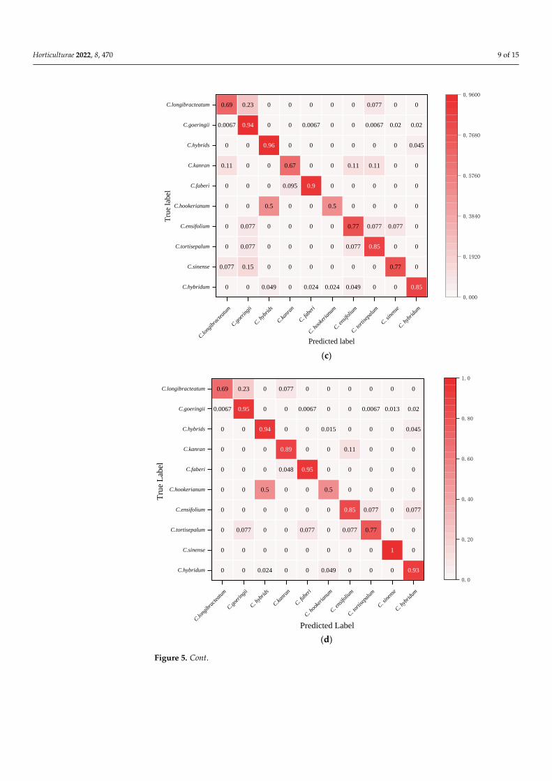
The visual confusion matrix was used to count the classification results of differentCymbidium species (Figure 5). The true category (ordinates) and the predicted category (ab-scissa) were compared to obtain the classification rate of each species. The GL-CNN modelhas the highest prediction accuracy for C. faberi and C. hookerianum, with an accuracy rate of100%, followed by C. hybridum, with an accuracy rate of 98% (Figure 5a). From the numeri-cal distribution of the confusion matrix, it can be observed that all models have achievedhigh classification accuracy on C. hybrids, and their average classification rates have reached95.6%. In addition, there have been more misclassifications between C. goeringii, C. longi-bracteatum, and C. tortisepalum. In general, the model GL-CNN built by this project hasachieved a high individual classification rate in most orchid species recognition. The recog-nition performance of VGG16 is poor, and there is a serious misclassification phenomenon.

Horticulturae 2022, 8, 470 8 of 15

Horticulturae 2022, 8, x FOR PEER REVIEW 8 of 15

0 0 0 0 0 0.024 0 0 0 0.98

0 0 0 0 0 0 0 0 1 0

0 0 0 0 0 0 0.15 0.85 0 0

0 0 0 0 0 0 0.77 0.077 0.077 0.077

0 0 0 0 0 1 0 0 0 0

0 0 0 0 1 0 0 0 0 0

0 0 0 0.89 0 0 0 0 0.11 0

0 0 0.96 0 0 0 0 0 0 0.045

0.0067 0.96 0.013 0 0.0067 0 0 0 0.0067 0.0067

0.69 0.23 0 0 0 0 0 0 0.077 0

C.lo

ngib

ract

eatu

m

C.g

oering

ii

C. h

ybrids

C.kan

ran

C. f

aber

i

C. h

ooke

rian

um

C. e

nsifo

lium

C. t

ortis

epal

um

C. s

inen

se

C. h

ybridu

m

C.hybridum

C.sinense

C.tortisepalum

C.ensifolium

C.hookerianum

C.faberi

C.kanran

C.hybrids

C.goeringii

C.longibracteatum

0

0.19

0.39

0.58

0.78

0.97

Tru

e L

abel

Predicted Label

(a)

0 0 0.024 0 0 0 0 0 0 0.98

0 0 0 0 0 0 0 0 1 0

0 0.077 0 0 0 0 0.23 0.69 0 0

0 0 0 0 0 0 0.69 0.077 0 0.23

0 0 0.5 0 0 0.5 0 0 0 0

0 0 0 0 1 0 0 0 0 0

0 0 0 0.56 0 0 0.33 0 0.11 0

0 0 0.96 0 0 0 0 0 0 0.23

0.013 0.93 0.013 0 0.0067 0 0.0067 0.013 0.0067 0.0067

0.46 0.38 0 0.077 0 0 0.077 0 0 0

C.lo

ngib

ract

eatu

m

C.g

oering

ii

C. h

ybrids

C.kan

ran

C. f

aber

i

C. h

ooke

rian

um

C. e

nsifo

lium

C. t

ortis

epal

um

C. s

inen

se

C. h

ybridu

m

C.hybridum

C.sinense

C.tortisepalum

C.ensifolium

C.hookerianum

C.faberi

C.kanran

C.hybrids

C.goeringii

C.longibracteatum

0.000

0.2000

0.4000

0.6000

0.8000

1.000

Tru

e L

abel

Predicted Label (b)

Figure 5. Cont.

Horticulturae 2022, 8, 470 9 of 15Horticulturae 2022, 8, x FOR PEER REVIEW 9 of 15

(c)

0 0 0.024 0 0 0.049 0 0 0 0.93

0 0 0 0 0 0 0 0 1 0

0 0.077 0 0 0.077 0 0.077 0.77 0 0

0 0 0 0 0 0 0.85 0.077 0 0.077

0 0 0.5 0 0 0.5 0 0 0 0

0 0 0 0.048 0.95 0 0 0 0 0

0 0 0 0.89 0 0 0.11 0 0 0

0 0 0.94 0 0 0.015 0 0 0 0.045

0.0067 0.95 0 0 0.0067 0 0 0.0067 0.013 0.02

0.69 0.23 0 0.077 0 0 0 0 0 0

C.lo

ngib

ract

eatu

m

C.g

oering

ii

C. h

ybrids

C.kan

ran

C. f

aber

i

C. h

ooke

rian

um

C. e

nsifo

lium

C. t

ortis

epal

um

C. s

inen

se

C. h

ybridu

m

C.hybridum

C.sinense

C.tortisepalum

C.ensifolium

C.hookerianum

C.faberi

C.kanran

C.hybrids

C.goeringii

C.longibracteatum

0.0

0.20

0.40

0.60

0.80

1.0

Tru

e L

abel

Predicted Label (d)

0 0 0.049 0 0.024 0.024 0.049 0 0 0.85

0.077 0.15 0 0 0 0 0 0 0.77 0

0 0.077 0 0 0 0 0.077 0.85 0 0

0 0.077 0 0 0 0 0.77 0.077 0.077 0

0 0 0.5 0 0 0.5 0 0 0 0

0 0 0 0.095 0.9 0 0 0 0 0

0.11 0 0 0.67 0 0 0.11 0.11 0 0

0 0 0.96 0 0 0 0 0 0 0.045

0.0067 0.94 0 0 0.0067 0 0 0.0067 0.02 0.02

0.69 0.23 0 0 0 0 0 0.077 0 0

C.lo

ngib

ractea

tum

C.g

oering

ii

C. h

ybrids

C.kan

ran

C. f

aber

i

C. h

ooke

rian

um

C. e

nsifo

lium

C. t

ortis

epal

um

C. s

inen

se

C. h

ybridu

m

C.hybridum

C.sinense

C.tortisepalum

C.ensifolium

C.hookerianum

C.faberi

C.kanran

C.hybrids

C.goeringii

C.longibracteatum

0.000

0.1920

0.3840

0.5760

0.7680

0.9600

Tru

e la

bel

Predicted label

Figure 5. Cont.

Horticulturae 2022, 8, 470 10 of 15Horticulturae 2022, 8, x FOR PEER REVIEW 10 of 15

0 0 0.049 0 0 0 0 0 0 0.95

0 0.077 0 0 0 0 0 0.077 0.85 0

0 0.15 0 0 0.077 0 0.15 0.62 0 0

0 0 0 0.077 0 0 0.77 0 0.077 0.077

0.5 0 0.5 0 0 0 0 0 0 0

0 0.048 0 0.19 0.76 0 0 0 0 0

0 0 0 0.78 0.11 0 0.11 0 0 0

0 0 0.96 0 0 0 0 0 0 0.045

0.0067 0.15 0.013 0 0.033 0 0.0067 0 0.0067 0

0.62 0.23 0 0.077 0 0 0 0.077 0 0

C.lo

ngib

ract

eatu

m

C.g

oering

ii

C. h

ybrids

C.kan

ran

C. f

aber

i

C. h

ooke

rian

um

C. e

nsifo

lium

C. t

ortis

epal

um

C. s

inen

se

C. h

ybridu

m

C.hybridum

C.sinense

C.tortisepalum

C.ensifolium

C.hookerianum

C.faberi

C.kanran

C.hybrids

C.goeringii

C.longibracteatum

0.000

0.1920

0.3840

0.5760

0.7680

0.9600

Tru

e L

abel

Predicted Label

(e)

Figure 5. Test set confusion matrix: (a) GL-CNN; (b) AlexNet; (c) ResNet; (d) GoogleNet; (e)

VGGNet.

Figure 6 shows the precision, recall, and F1-score of 5 models for classifying 10

Cymbidium species. Among them, the precision, recall, and F1-score of each model on

C.goeringii and C. hybrids all reached high values. On the contrary, the precision, recall,

and F1-score of the five models on the C. hookerianum are quite different. GL-CNN has the

highest precision, with an average of 89%. ResNet’s average precision is the lowest, only

78%, indicating that there are many samples misclassified under this method. Using the

AlexNet model, many samples were misclassified to other varieties (the average recall

rate was 0.78) because the differences between the samples were small, and there was a

certain degree of difficulty in recognition. The precision and recall rate of different models

are quite different, which indicates that the recognition difference of each model is more

prominent in the categories that are more difficult to distinguish, showing a certain degree

of unstable performance. In addition, GL-CNN showed high precision and recall rates in

10 different species of Cymbidium, indicating its strong ability to extract nuances.

Table 2 lists the average accuracy of the five models in order to further and

comprehensively evaluate the effectiveness of the model. It can be observed from the table

that GL-CNN has achieved the highest average accuracy of 94.13%. Compared with other

models, GL-CNN has greatly improved the accuracy of classification. Correspondingly,

VGG16 only achieves an average accuracy of 88.60%, which is significantly lower than

GL-CNN.

Figure 5. Test set confusion matrix: (a) GL-CNN; (b) AlexNet; (c) ResNet; (d) GoogleNet; (e) VGGNet.

Figure 6 shows the precision, recall, and F1-score of 5 models for classifying 10 Cymbidiumspecies. Among them, the precision, recall, and F1-score of each model on C. goeringii andC. hybrids all reached high values. On the contrary, the precision, recall, and F1-score of thefive models on the C. hookerianum are quite different. GL-CNN has the highest precision,with an average of 89%. ResNet’s average precision is the lowest, only 78%, indicating thatthere are many samples misclassified under this method. Using the AlexNet model, manysamples were misclassified to other varieties (the average recall rate was 0.78) because thedifferences between the samples were small, and there was a certain degree of difficultyin recognition. The precision and recall rate of different models are quite different, whichindicates that the recognition difference of each model is more prominent in the categoriesthat are more difficult to distinguish, showing a certain degree of unstable performance.In addition, GL-CNN showed high precision and recall rates in 10 different species ofCymbidium, indicating its strong ability to extract nuances.

Table 2 lists the average accuracy of the five models in order to further and compre-hensively evaluate the effectiveness of the model. It can be observed from the table thatGL-CNN has achieved the highest average accuracy of 94.13%. Compared with other mod-els, GL-CNN has greatly improved the accuracy of classification. Correspondingly, VGG16only achieves an average accuracy of 88.60%, which is significantly lower than GL-CNN.

Table 2. Average accuracy of each model.

GL-CNN AlexNet ResNet GoogleNet VGGNet

Averageaccuracy (%) 94.13 90.06 89.47 92.15 88.60

Horticulturae 2022, 8, 470 11 of 15

Horticulturae 2022, 8, x FOR PEER REVIEW 11 of 15

C.long

ibra

ctea

tum

C.goe

ringi

i

C.hyb

rids

C.kan

ran

C.fabe

ri

C.hoo

keria

num

C.kan

ran

C.torti

sepa

lum

C.sine

nse

C.hyb

ridum

0.0

0.2

0.4

0.6

0.8

1.0

(a)

GL-CNN

AlexNet

ResNet

GoogleNet

VGG-16

Pre

cisi

on

C.long

ibra

ctea

tum

C.goe

ringi

i

C.hyb

rids

C.kan

ran

C.fabe

ri

C.hoo

keria

num

C.kan

ran

C.torti

sepa

lum

C.sine

nse

C.hyb

ridum

0.0

0.2

0.4

0.6

0.8

1.0

Rec

all

(b)

GL-CNN

AlexNet

ResNet

GoogleNet

VGG-16

Figure 6. Cont.

Horticulturae 2022, 8, 470 12 of 15

Horticulturae 2022, 8, x FOR PEER REVIEW 12 of 15

C.lo

ngib

ract

eatu

m

C.g

oerin

gii

C.h

ybrid

s

C.k

anra

n

C.fa

beri

C.h

ooke

rianu

m

C.k

anra

n

C.to

rtise

palu

m

C.si

nens

e

C.h

ybrid

um

0.0

0.2

0.4

0.6

0.8

1.0

F1-s

core

(c)

GL-CNN

AlexNet

ResNet

GoogleNet

VGG-16

Figure 6. Precision (a), recall (b), and F1-score (c) of each model on different Cymbidium species.

Table 2. Average accuracy of each model.

GL-CNN AlexNet ResNet GoogleNet VGGNet

Average accuracy (%) 94.13 90.06 89.47 92.15 88.60

4. Discussion

CNN is a method that combines an artificial neural network and deep learning with

good fault tolerance and adaptability [42]. At the same time, it also has the advantages of

automatic feature extraction, weight sharing, and a good combination of input image and

network structure [27]. It is widely used in plant species identification, pest identification,

weed identification, and other fields [43–45]. Existing CNN-based classification methods

mainly focus on single-scale image data sets [27]. Therefore, there is an urgent need to

design a fusion network that integrates the advantages of multiple features, which will

greatly improve classification performance. This research proposed a two-scale CNN

model, GL-CNN, which can extract features of different granularities from images of two

scales, thereby enriching useful feature information, and ultimately improving the

recognition ability of the model [26,27]. Researchers found that increasing the number of

layers and units in the network will bring significant performance improvements, but it

is prone to overfitting, explosion, or the disappearance of gradients [26]. To solve the

above problems, a compact bilinear pooling method was proposed by Gao et al. [46],

which can reduce the dimensionality while maintaining accuracy. Our experiment used a

cascade fusion strategy to fit the two-scale features obtained from the two branches.

Meanwhile, ReLU6, dropout, and other methods were used to alleviate potential

overfitting problems. In the process of network training, dropout reduces the running

time by randomly ignoring a certain proportion of hidden layer nodes, which can

effectively reduce the interdependence between neurons, thereby extracting independent

important features and inhibiting network overfitting.

In model training, the choice of feature extractor can affect the accuracy and speed of

model detection. As the number of feature extractor layers increases, the network can

extract higher-dimensional sample features, but the increase in network depth will affect

Figure 6. Precision (a), recall (b), and F1-score (c) of each model on different Cymbidium species.

4. Discussion

CNN is a method that combines an artificial neural network and deep learning withgood fault tolerance and adaptability [42]. At the same time, it also has the advantages ofautomatic feature extraction, weight sharing, and a good combination of input image andnetwork structure [27]. It is widely used in plant species identification, pest identification,weed identification, and other fields [43–45]. Existing CNN-based classification methodsmainly focus on single-scale image data sets [27]. Therefore, there is an urgent need todesign a fusion network that integrates the advantages of multiple features, which willgreatly improve classification performance. This research proposed a two-scale CNN model,GL-CNN, which can extract features of different granularities from images of two scales,thereby enriching useful feature information, and ultimately improving the recognitionability of the model [26,27]. Researchers found that increasing the number of layers andunits in the network will bring significant performance improvements, but it is prone tooverfitting, explosion, or the disappearance of gradients [26]. To solve the above problems,a compact bilinear pooling method was proposed by Gao et al. [46], which can reducethe dimensionality while maintaining accuracy. Our experiment used a cascade fusionstrategy to fit the two-scale features obtained from the two branches. Meanwhile, ReLU6,dropout, and other methods were used to alleviate potential overfitting problems. In theprocess of network training, dropout reduces the running time by randomly ignoring acertain proportion of hidden layer nodes, which can effectively reduce the interdepen-dence between neurons, thereby extracting independent important features and inhibitingnetwork overfitting.

In model training, the choice of feature extractor can affect the accuracy and speedof model detection. As the number of feature extractor layers increases, the networkcan extract higher-dimensional sample features, but the increase in network depth willaffect the update signal of each layer and affect detection accuracy [47,48]. As classicfeature extractors, AlexNet, ResNet, GoogleNet, and VGGNet are mostly used for imageclassification and recognition [48,49]. This study has shown that compared with the fourtypical models, GL-CNN has obvious accuracy and computational advantages, and themodel accuracy is as high as 94%. An unexpected phenomenon is that the two excellentmodels (VGGNet and ResNet) did not achieve the desired performance, especially VGGNet,which obtained the lowest results, with a model accuracy of only 88.6%. The reason for

Horticulturae 2022, 8, 470 13 of 15

this phenomenon is that the VGGNet training speed is very slow, and the weight of thenetwork architecture itself is very large. In the case of many parameters and insufficientimage data, the excellent classification effect cannot be exerted [49,50]. ResNet’s networkconnection is also very complicated and requires a lot of calculations. Therefore, they needa large data set to complete the convergence of the model [50]. In contrast, GoogLeNet,and AlexNet contain fewer parameters, a relatively simpler structure, and better trainingeffects than VGGNet and ResNet [27]. As the best training model, GL-CNN has a slightadvantage over GoogleNet in accuracy. The parameters and calculations of GL-CNNare significantly smaller, and it is easy to construct and apply. When the orchid imagewith more background information is adjusted to 224 × 224, a great deal of fine-grainedinformation will be lost, which prevents the network from learning more in-depth andsufficient details. This situation can lead to poor network performance. GL-CNN can obtainglobal and local information and cascade the two parts together to extract detailed contextfeatures, which helps to expand the input features and improve classification accuracy.

Deep learning is still data-driven, and the size and quality of the data set will directlyaffect the effectiveness of network training [26]. Due to the limitation of the data set size, itmay be difficult to train CNN. This study found that the precision, recall, and F1-score ofeach model on C. hookerianum are quite different. This is due to the small sample size ofC. hookerianum, which makes the stability performance of the model different. Therefore,the training model is not sensitive enough to recognize the experimental samples. Byincreasing the number of such images, the compatibility of the classification model fordifferent Cymbidium species can be improved.

5. Conclusions

In this study, a Cymbidium classification method based on the GL-CNN was proposed.It consists of two CNN networks with comparable weight, which helps expand the inputfeatures and improve classification accuracy. The cascade fusion strategy was used to fitthe multiscale features obtained from the two branches. ReLU6 and dropout were used toprevent gradient explosion and alleviate the problem of overfitting. The end-to-end trainingwas realized, and the robustness of the model was enhanced. Comparing GL-CNN withfour classic models (AlexNet, ResNet50, GoogleNet, and VGG16), the results showed thatGL-CNN achieved the highest classification prediction accuracy with a value of 94.13%.

In summary, the GL-CNN model used in this paper integrates multiscale informationthrough the network, expands the number of features, has high detection accuracy, and caneffectively identify different species of Cymbidium.

Author Contributions: Q.F. and C.L. conceived the ideas and designed the methodology; Q.F.collected and analyzed the data and wrote the manuscript; C.L. guided the data analysis andreviewed the manuscripts; F.Z., R.R., L.Q., X.Z. and C.L. supervised all stages of the experiment. Allauthors have read and agreed to the published version of the manuscript.

Funding: This research was supported by the Hangzhou Agriculture and Social DevelopmentProject (20201203B104).

Institutional Review Board Statement: Not applicable.

Informed Consent Statement: Not applicable.

Data Availability Statement: Data are contained within the article.

Conflicts of Interest: The authors declare no conflict of interest.

Horticulturae 2022, 8, 470 14 of 15

References1. Dressler, R.L. Phylogeny and Classification of the Orchid Family; Cambridge University Press: Cambridge, UK, 1993.2. Sharma, S.K.; Rajkumari, K.; Kumaria, S.; Tandon, P.; Rao, S.R. Karyo-morphological characterization of natural genetic variation

in some threatened Cymbidium species of Northeast India. Caryologia 2010, 63, 99–105. [CrossRef]3. Lee, Y.-M.; Kim, M.-S.; Lee, S.-I.; Kim, J.-B. Review on breeding, tissue culture and genetic transformation systems in Cymbidium.

J. Plant Biotechnol. 2010, 37, 357–369. [CrossRef]4. Wang, H.-Z.; Lu, J.-J.; Hu, X.; Liu, J.-J. Genetic variation and cultivar identification in Cymbidium ensifolium. Plant Syst. Evol. 2011,

293, 101–110. [CrossRef]5. Ning, H.; Ao, S.; Fan, Y.; Fu, J.; Xu, C. Correlation analysis between the karyotypes and phenotypic traits of Chinese cymbidium

cultivars. Hortic. Environ. Biotechnol. 2018, 59, 93–103. [CrossRef]6. Guo, F.; Niu, L.-X.; Zhang, Y.-L. Phenotypic Variation of Natural Populations of Cymbidium faberi in Zhashui. North Hortic. 2010,

18, 91–93.7. Sharma, S.K.; Kumaria, S.; Tandon, P.; Rao, S.R. Assessment of genetic variation and identification of species-specific ISSR markers

in five species of Cymbidium (Orchidaceae). J. Plant Biochem. Biotechnol. 2013, 22, 250–255. [CrossRef]8. Lu, J.; Hu, X.; Liu, J.; Wang, H. Genetic diversity and population structure of 151 Cymbidium sinense cultivars. J. Hortic. For. 2011,

3, 104–114.9. Lee, D.-G.; Koh, J.-C.; Chung, K.-W. Determination and application of combined genotype of simple sequence repeats (SSR) DNA

marker for cultivars of Cymbidium goeringii. Hortic. Sci. Technol. 2012, 30, 278–285. [CrossRef]10. Obara-Okeyo, P.; Kako, S. Genetic diversity and identification of Cymbidium cultivars as measured by random amplified

polymorphic DNA (RAPD) markers. Euphytica 1998, 99, 95–101. [CrossRef]11. LeCun, Y.; Bengio, Y.; Hinton, G. Deep learning. Nature 2015, 521, 436–444. [CrossRef]12. Tian, C.; Xu, Y.; Fei, L.; Yan, K. Deep learning for image denoising: A survey. In Proceedings of the International Conference on

Genetic and Evolutionary Computing, Springer, Singapore, 14–17 December 2018; pp. 563–572.13. Albawi, S.; Mohammed, T.A.; Al-Zawi, S. Understanding of a convolutional neural network. In Proceedings of the 2017

International Conference on Engineering and Technology (ICET), Antalya, Turkey, 21–23 August 2017; pp. 1–6.14. Cengil, E.; Çinar, A.; Güler, Z. A GPU-based convolutional neural network approach for image classification. In Proceedings of

the 2017 International Artificial Intelligence and Data Processing Symposium (IDAP), Malatya, Turkey, 16–17 September 2017;pp. 1–6.

15. Dyrmann, M.; Karstoft, H.; Midtiby, H.S. Plant species classification using deep convolutional neural network. Biosys. Eng. 2016,151, 72–80. [CrossRef]

16. Yalcin, H.; Razavi, S. Plant classification using convolutional neural networks. In Proceedings of the 2016 Fifth InternationalConference on Agro-Geoinformatics (Agro-Geoinformatics), Tianjin, China, 18–20 July 2016; pp. 1–5.

17. Ma, J.; Du, K.; Zheng, F.; Zhang, L.; Gong, Z.; Sun, Z. A recognition method for cucumber diseases using leaf symptom imagesbased on deep convolutional neural network. Comput. Electron. Agric. 2018, 154, 18–24. [CrossRef]

18. Patel, I.; Patel, S. An Optimized Deep Learning Model for Flower Classification Using NAS-FPN and Faster R-CNN. Int. J. Sci.Technol. Res. 2020, 9, 5308–5318.

19. Liu, Y.H. Feature extraction and image recognition with convolutional neural networks. J. Phys. Conf. Ser. 2018, 1087, 062032.[CrossRef]

20. Workman, S.; Jacobs, N. On the location dependence of convolutional neural network features. In Proceedings of the IEEEConference on Computer Vision and Pattern Recognition Workshops, Boston, MA, USA, 7–12 June 2015; pp. 70–78.

21. Li, W.; Wu, G.; Zhang, F.; Du, Q. Hyperspectral image classification using deep pixel-pair features. IEEE Trans. Geosci. RemoteSens. 2016, 55, 844–853. [CrossRef]

22. Hiary, H.; Saadeh, H.; Saadeh, M.; Yaqub, M. Flower classification using deep convolutional neural networks. IET Comput. Vis.2018, 12, 855–862. [CrossRef]

23. Dias, P.A.; Tabb, A.; Medeiros, H. Apple flower detection using deep convolutional networks. Comput. Ind. 2018, 99, 17–28.[CrossRef]

24. Alaslani, M.G. Convolutional neural network based feature extraction for iris recognition. Int. J. Comput. Sci. Inf. Technol. (IJCSIT)2018, 10, 65–78. [CrossRef]

25. Huang, K.; Liu, X.; Fu, S.; Guo, D.; Xu, M. A lightweight privacy-preserving CNN feature extraction framework for mobilesensing. IEEE Trans. Dependable Secur. Comput. 2019, 18, 1441–1455. [CrossRef]

26. Xie, G.-S.; Zhang, X.-Y.; Yang, W.; Xu, M.; Yan, S.; Liu, C.-L. LG-CNN: From local parts to global discrimination for fine-grainedrecognition. Pattern Recognit. 2017, 71, 118–131. [CrossRef]

27. Hao, X.; Jia, J.; Khattak, A.M.; Zhang, L.; Guo, X.; Gao, W.; Wang, M. Growing period classification of Gynura bicolor DC usingGL-CNN. Comput. Electron. Agric. 2020, 174, 105497. [CrossRef]

28. Simonyan, K.; Zisserman, A. Very deep convolutional networks for large-scale image recognition. arXiv 2014, arXiv:1409.1556.29. Chao, X.; Sun, G.; Zhao, H.; Li, M.; He, D. Identification of apple tree leaf diseases based on deep learning models. Symmetry 2020,

12, 1065. [CrossRef]30. Neupane, B.; Horanont, T.; Aryal, J. Deep Learning-Based Semantic Segmentation of Urban Features in Satellite Images: A Review

and Meta-Analysis. Remote Sens. 2021, 13, 808. [CrossRef]

Horticulturae 2022, 8, 470 15 of 15

31. Zhou, Q.; Situ, Z.; Teng, S.; Chen, G. Convolutional Neural Networks—Based Model for Automated Sewer Defects Detection andClassification. J. Water Resour. Plan. Manag. 2021, 147, 04021036. [CrossRef]

32. Huang, K.; Li, C.; Zhang, J.; Wang, B. Cascade and Fusion: A Deep Learning Approach for Camouflaged Object Sensing. Sensors2021, 21, 5455. [CrossRef]

33. Lin, G.; Shen, W. Research on convolutional neural network based on improved Relu piecewise activation function. ProcediaComput. Sci. 2018, 131, 977–984. [CrossRef]

34. Agarap, A.F. Deep learning using rectified linear units (relu). arXiv 2018, arXiv:1803.08375.35. Srivastava, N.; Hinton, G.; Krizhevsky, A.; Sutskever, I.; Salakhutdinov, R. Dropout: A simple way to prevent neural networks

from overfitting. J. Mach. Learn. Res. 2014, 15, 1929–1958.36. Hu, K.; Zhang, Z.; Niu, X.; Zhang, Y.; Cao, C.; Xiao, F.; Gao, X. Retinal vessel segmentation of color fundus images using multiscale

convolutional neural network with an improved cross-entropy loss function. Neurocomputing 2018, 309, 179–191. [CrossRef]37. Dozat, T. Incorporating nesterov momentum into adam. In Proceedings of the 4th International Conference on Learning

Representations, Workshop Track, Caribe Hilton, San Juan, Puerto Rico, 2–4 May 2016.38. Yu, W.; Yang, K.; Bai, Y.; Xiao, T.; Yao, H.; Rui, Y. Visualizing and comparing AlexNet and VGG using deconvolutional layers. In

Proceedings of the 33rd International Conference on International Conference on Machine Learning, New York, NY, USA, 19–24June 2016.

39. Ballester, P.; Araujo, R.M. On the performance of GoogLeNet and AlexNet applied to sketches. In Proceedings of the ThirtiethAAAI Conference on Artificial Intelligence, Phoenix, AZ, USA, 12–17 February 2016.

40. Gao, M.; Chen, J.; Mu, H.; Qi, D. A Transfer Residual Neural Network Based on ResNet-34 for Detection of Wood Knot Defects.Forests 2021, 12, 212. [CrossRef]

41. Yacouby, R.; Axman, D. Probabilistic Extension of Precision, Recall, and F1 Score for More Thorough Evaluation of ClassificationModels. In Proceedings of the First Workshop on Evaluation and Comparison of NLP Systems; Association for Computational Linguistics:Stroudsburg, PA, USA, 2020; Volume 202, pp. 79–91.

42. Azman, A.A.; Ismail, F.S. Convolutional Neural Network for Optimal Pineapple Harvesting. ELEKTRIKA-J. Electr. Eng. 2017,16, 1–4.

43. Saleem, G.; Akhtar, M.; Ahmed, N.; Qureshi, W.S. Automated analysis of visual leaf shape features for plant classification. Comput.Electron. Agric. 2019, 157, 270–280. [CrossRef]

44. Liu, J.; Pi, J.; Xia, L. A novel and high precision tomato maturity recognition algorithm based on multi-level deep residual network.Multimed. Tools Appl. 2020, 79, 9403–9417. [CrossRef]

45. Esgario, J.G.M.; Krohling, R.A.; Ventura, J.A. Deep learning for classification and severity estimation of coffee leaf biotic stress.Comput. Electron. Agric. 2020, 169, 105162. [CrossRef]

46. Gao, Y.; Beijbom, O.; Zhang, N.; Darrell, T. Compact bilinear pooling. In Proceedings of the 2016 IEEE Conference on ComputerVision and Pattern Recognition (CVPR), Las Vegas, NV, USA, 27–30 June 2016; pp. 317–326.

47. Yuan, Z.-W.; Zhang, J. Feature extraction and image retrieval based on AlexNet. In Proceedings of the Eighth InternationalConference on Digital Image Processing (ICDIP 2016), Chengdu, China, 20–22 May 2016; p. 100330E.

48. Thenmozhi, K.; Reddy, U.S. Crop pest classification based on deep convolutional neural network and transfer learning. Comput.Electron. Agric. 2019, 164, 104906. [CrossRef]

49. Sethy, P.K.; Barpanda, N.K.; Rath, A.K.; Behera, S.K. Nitrogen deficiency prediction of rice crop based on convolutional neuralnetwork. J. Ambient. Intell. Humaniz. Comput. 2020, 11, 5703–5711. [CrossRef]

50. Yaqoob, M.K.; Ali, S.F.; Bilal, M.; Hanif, M.S.; Al-Saggaf, U.M. ResNet Based Deep Features and Random Forest Classifier forDiabetic Retinopathy Detection. Sensors 2021, 21, 3883. [CrossRef]