Decoherence in a classically chaotic quantum system: Entropy production and quantum-classical correspondence

arX

iv:q

uant

-ph/

0106

090v

1 1

5 Ju

n 20

01

Decoherence in a classically chaotic quantum system: entropy production and

quantum–classical correspondence

Diana Monteoliva ∗ and Juan Pablo Paz †

Departamento de Fisica Juan Jose Giambiagi, FCEyN, UBA, Pabellon 1, Ciudad Universitaria, 1428 Buenos Aires, Argentina

(February 1, 2008)

We study the decoherence process for an open quantum system which is classically chaotic(a quartic double well with harmonic driving coupled to a sea of harmonic oscillators). Wecarefully analyze the time dependence of the rate of entropy production showing that it hastwo relevant regimes: For short times it is proportional to the diffusion coefficient (fixed bythe system–environment coupling strength). For longer times (but before equilibration) it isfixed by dynamical properties of the system (and is related to the Lyapunov exponent). Thenature of the transition time between both regimes is investigated and the issue of quantumto classical correspondence is addressed. Finally, the impact of the interaction with theenvironment on coherent tunneling is analyzed.

PACS numbers: 03.65.Bz

I. INTRODUCTION

The process of decoherence has been identified as oneof the main ingredients to explain the origin of the classi-cal world from a fundamentally quantum substrate [1,2].In fact, according to the decoherence paradigm, classical-ity is an emergent property imposed upon open systemsby the interaction with an external environment. In allrealistic situations this interaction, as it became clearin recent years, generates a de facto superselection rulethat prevents the stable existence of most of the statesin the Hilbert space of the system. Only a small set ofstates of the system are relatively stable, they are theso–called pointer states [3,4]. While pointer states areminimally disturbed by the interaction with the environ-ment, coherent superpositions of such states are rapidlydestroyed by decoherence. Thus, this process transformsthe quantum state of the system into a mixture of pointerstates. In recent years the study of the physics of deco-herence has helped to clarify many interesting featuresof this process. For example: the nature of the decoher-ence timescales is now well understood [5,6]; the essen-tial features of the process by which the pointer statesare dynamically selected by the environment are well un-derstood [7–9] (see [10] for a recent review). Moreover(and most notably) the study of decoherence became ac-tive from the experimental point of view where the firstgeneration of experiments exploring the fuzzy boundarybetween the quantum and the classical world are alreadystarting to produce interesting results [11–13].

Over the course of these studies it became clear thatthe decoherence process has very peculiar features forquantum systems whose classical analogues are chaotic.

∗[email protected]†[email protected]

In fact, for such systems decoherence seems to be abso-lutely essential to restore the validity of the correspon-dence principle violated for very short times (the breakuptime depends logarithmically on the Planck constant)[14–17]. The reason for the breakdown of the correspon-dence principle for chaotic systems (and for its restora-tion due to decoherence) can be understood as follows:For these type of systems, quantum evolution continu-ously generates a coherent spreading of the wave functionover large scales both in position and momentum. Thus,a classically chaotic Hamiltonian generates a quantumevolution which typically produces “Schrodinger cat”type states, i.e. starting from a state which is well lo-calized both in position and momentum the quantumevolution produces a state which is highly delocalized ex-hibiting strong interference effects. One may be temptedto argue that this effect, while existing, could not be rel-evant for large macroscopic systems. But, surprisinglyor not, even for as large an object as the components ofthe solar system which are chaotic, quantum predictionsare alarming: On a timescale th as short as a month forHyperion, one of the moons of Saturn whose chaotic tum-bling motion has been analyzed [18], the initial Gaussianstate of this celestial body would spread over distancesof the order of the radius of its orbit! [15]. Thus, thoughplanetary dynamics appears to be a safe distance awayfrom the quantum regime, as a consequence of the chaotic

character of the evolution, a simple application of theSchrodinger equation would tell us that this is not thecase. In fact, the macroscopic size of a system (be it aplanet or a cat) is not enough to guarantee its classical-ity. Thus, classicality in such system would emerge onlyas a consequence of decoherence, as we will later discussin this paper.

The reason why a classically chaotic Hamiltonian gen-erates highly nonclassical states can be related to thefact that chaotic dynamics is characterized by exponen-tial divergence of neighboring trajectories. To be able

1

to present this argument, based on the notion of trajec-tories, it is better to formulate quantum mechanics inphase space (a task that can be accomplished by using,for example, the Wigner distribution [19] to representthe quantum state). In fact, if one prepares a quan-tum system in a classical state, with a Wigner functionwell localized in phase space and smooth over regionswith an area which is large compared with the Planckconstant, it will initially evolve following classical tra-jectories in phase space. Therefore, after some charac-teristic time the initially smooth wave packet will be-come stretched in one (unstable) direction and, due tothe conservation of volume, squeezed in the other (sta-ble) one. This squeezing and stretching is also accompa-nied by the folding of classical trajectories which, in thefully chaotic regime, tend to fill all the available phasespace. The combination of these three related effects –squeezing, stretching and folding – forces the system toexplore the quantum regime. Thus, being stretched inone direction the wavepacket becomes delocalized and, asa consequence of folding, quantum interference betweenthe different pieces of the wavepacket, which remain co-herent over long distances, develops. The timescale forthe correspondence breakdown can be also estimated viaa simple argument: As the wave packet squeezes expo-nentially fast in one direction (momentum, for example),σp(t) = σp(0)e−λt, it will correspondingly become coher-ent over a distance that can be estimated from Heisen-berg’s principle as l(t) ≥ h

σp(0)eλt. When the spread-

ing is comparable with the scale χ where the potentialis significantly nonlinear, folding will start to apprecia-tively affect the evolution of the wave packet and longrange quantum interference will set in. This time, whichcorresponds approximately to the time when quantumand classical expectation values start to differ from each

other, can therefore be estimated as th = λ−1ln(σp(0)χ

h )(note that the quantity χ can be as large as the size ofthe orbit of a planet [15,20] for gravitational potential).

But nothing of this sort is evident in real life: themoon of Saturn does not spread over large distances andthe correspondence principle seems to be valid for macro-scopic objects that, like Hyperion, behave according toclassical laws. So, how can classical mechanics be re-covered? Decoherence is a way out of this problem. Asthe system evolves while continuously interacting withits environment, it may become classical if the interac-tion is such that it continuously destroys the quantum co-herence which are dynamically generated by the chaoticevolution. The role of decoherence in recovering the cor-respondence principle has been suggested some time ago[15] and numerically analyzed more recently [16].

But, as originally suggested by Zurek and one of us[14], the decoherence process for classically chaotic sys-tems has another very important feature, that comes asa bonus. The interaction with the environment destroysthe purity of the system since they become entangled.Thus, information initially stored in the system leaks

into the environment and therefore decoherence is al-ways accompanied with entropy production. This is, ofcourse, true both for classically regular and classicallychaotic systems. But what distinguishes chaotic systemsis the existence of a robust range of parameters for whichthe rate at which the information flows from the systeminto the environment (i.e., the rate of entropy produc-tion) becomes entirely independent of the strength of thecoupling between the system and the environment andis dictated by dynamical properties of the system only(i.e., by averaged Lyapunov exponents). The reason forthis can also be understood using a simple (clearly over-simplified) argument. The decoherence process destroysquantum interference between distant pieces of the wavepacket of the system and puts a lower bound on thesmall scale structure that the Wigner function can de-velop. Thus, the Wigner function can no longer squeezeindefinitely but it stops contracting as a consequence ofthe interaction with the environment, which can be typ-ically modelled as diffusion [22–24]. As a consequence ofthis, and due to the fact that expansion (or folding) isnot substantially affected by diffusion, the entropy of thesystem grows at a rate which is essentially fixed by theaverage rate of expansion given by the average Lyapunovexponent. In this regime, the entropy production ratebecomes independent of the diffusion constant (which,on the other hand, is responsible for the whole process).This result was first conjectured in [14]. More recently,numerical evidence supporting the conjecture was pre-sented [17,25–28]. The aim of this paper is to presentsolid numerical evidence supporting this result and tostudy other related aspects of decoherence for a particu-lar chaotic system. As will become clear later, our studiesshow that the time dependence of the entropy productionrate has two rather different regimes. First, there is aninitial transient where the entropy production rate is pro-portional to the system–environment coupling strength(i.e., in this initial regime the rate behaves in the sameway as in the regular –non chaotic– case). Second, af-ter this initial transient the entropy production rate goesinto a regime where its value is fixed as conjectured in[14] by the Lyapunov exponents of the system and isindependent of the strength of the coupling to the envi-ronment. In our work we show that the transition timetc between both regimes is linearly dependent on the en-tropy of the initial state, and logarithmically dependenton the system–environment coupling strength.

Our aim in this paper is not to give an extensive list ofall relevant references connected to the study of dissipa-tive effects in classically chaotic quantum systems. How-ever, we believe it is worth pointing out that our workis by no means the first attempt to study these effectswhich, in connection to problems such as the impact ofnoise on localization, the appearence of classical featuresin phase space (like strange attractors, etc) were studiedin pioneering works several years ago (see for example[29]). As general source of reference in this area we rec-ommend to interesting books where one can find a rather

2

extended compilation of important works [30,31]. For ournumerical study we have chosen as nonlinear system thedriven quartic double well, described in detail in SectionII. We study the evolution of our system for very simple(Gaussian) initial conditions (i.e., initial conditions that,from a start, do no exhibit any quantum interference ef-fects) so as to focus our attention on the interplay be-tween two competing effects: generation and destructionof dynamically generated interferences. We also present,in Section II, a discussion of the breakdown of correspon-dence for chaotic systems. Then, on Section III the wayin which we model the interaction between our systemand an environment is presented with some detail. Wedo this by using two complementary approaches basedon master equations both giving consistent results butone of them enable the study of the evolution for longdynamical times, which is relevant for discussing the im-pact of decoherence on tunneling. Numerical results con-cerning the time dependence of the decoherence rate anda discussion of their relevance are presented in SectionIV. Finally, we discuss the impact of the interaction withthe environment on the tunneling phenomena in SectionV and we end with some concluding remarks on SectionVI.

II. EVOLUTION OF THE QUANTUM ISOLATED

SYSTEM

In this Section we study the dynamical behaviour ofan isolated quantum system with Hamiltonian

H0(x, p, t) =p2

2m− bx2 +

x4

64a+ sx cos(ωt), (1)

which corresponds to a harmonically driven quartic dou-ble well. This non-linear system has been extensivelystudied [32,33] in the literature. For s = 0 the systemis integrable and exhibits the generic phase space of abistable system. It has two stable fixed points at x =±

√

(32ba), p = 0 (with associated energy E = −16b2a)and one unstable fixed point at x = 0, p = 0 (withE = 0). The presence of the driving term introduces aninfinite number of primary resonance zones in the phasespace of the system. The tori near the separatrix of thenon-driven system (E = 0) and KAM invariant tori inthe region between resonance zones are progressively de-stroyed as the amplitude s of the driving increases. Thephase space of the system starts to look chaotic, present-ing in general a mixed nature as can be seen (for twosets of parameters) in Figure 1. The regions around thetwo stable fixed points and the chains of resonant islandsform regular regions where the dynamics of the systemis nearly integrable. The chaotic layers between regularregions develop from the homoclinic tangles, the intrin-cated interweaving of the stable and unstable manifoldsoriginated at the hyperbolic fixed points between the res-onant islands or the one at the origin. For small values

of the driving amplitude, chaotic layers are so thin thatonly those near the unstable fixed point of the integrablesystem can be seen in the stroboscopic phase space por-trait. As the value of s is increased these chaotic regionsgain in relevance while resonances other than the two firstones near the stable fixed points become in turn smallerand are almost invisible to the eye. For large values ofthe driving amplitude s the different chaotic layers mergeinto what is called the chaotic sea; the stable islands andtwo first resonant islands are much reduced (see Figure1a). In what follows we will choose parameters so thateither the majority of the phase space is chaotic, as inFigure 1b, where the stable islands around the stablefixed points of the integrable system have shrunken toinvisibility and only the two first resonance islands areseen, or the regular regions coexist with the chaotic seaas shown in Figure 1a.

FIG. 1. Stroboscopic phase space of the driven double wellwith parameters (a) m = 1, b = 10, a = 1/32, s = 1, ω = 5.35and (b) m = 1, b = 10, a = 1/32, s = 10, ω = 6.07. Theborders of the dark elipses represent contours of minimun un-certainty Gaussian initial conditions at 1/20 of its peak value,for x0 = −3.7, p0 = 0, σx = .05, σp = 1 on the leftmost islandand x0 = 1, p0 = 0, σ2

x = .05, σ2

p = .05 on the chaotic sea.

As we mentioned above, our aim is to follow the quan-tum evolution of initial states whose Wigner functionsare fully contained either in a regular island or in thechaotic sea, as illustrated in Figures 1a and 1b. This re-

3

quirement forces us to take values of h which are smallenough. Indeed, for the parameter set corresponding toFigure 1a, the leftmost regular island has an area whichis approximately given by A ∼ 6π. If we need stateswell localized within each region (the regular islands orthe chaotic sea) we need to compare this area with theone covered by the dark ellipses appearing in Figure 1,which are given by Ae = 2π ln(20)σxσp = π ln(20)h (i.e.,we consider initial states which are pure, minimal un-certainty, coherent states). Thus, a reasonable value forh (the one we choose) is h = 0.1 for the island to beabout 20 times larger than the extent of the initial state(for the parameters corresponding to Figure 1b a largervalue of h could also be chosen for our purposes). +We numerically solved the Schrodinger equation for thissystem evolving the above initial states using two differ-ent methods. First, we integrated this equation with astep by step algorithm using a high resolution spectralmethod [34]. Second, we solved the same equation ap-plying a numerical technique based on the use of Floquetstates [35]. This method consists of numerically find-ing eigenstates of the unitary evolution operator for oneperiod (Floquet states) which form a complete basis ofthe Hilbert space of the system. By expanding the ini-tial state on this basis, the solution of the Schrodingerequation becomes trivial [36]. Thus, all the difficultly ofthe method is hidden in finding the Floquet states (thesame applies when solving the Schrodinger equation fora time–independent Hamiltonian). We succesfully usedthis method for some parameter sets but did not apply itfor all cases of interest. In fact, the main difficulty of themethod is the number of Floquet states required to accu-rately expand the initial states shown in Figure 1, whichrapidly grow as h becomes small (for example, for theparameters of Figure 1b, with h = 0.1, one needs morethan 200 Floquet states to evolve the wave packet cen-tered in the chaotic sea). In what follows we will discussthe typical results one finds when solving the Schrodingerequation with the above initial states.

A. Initial states in a regular island

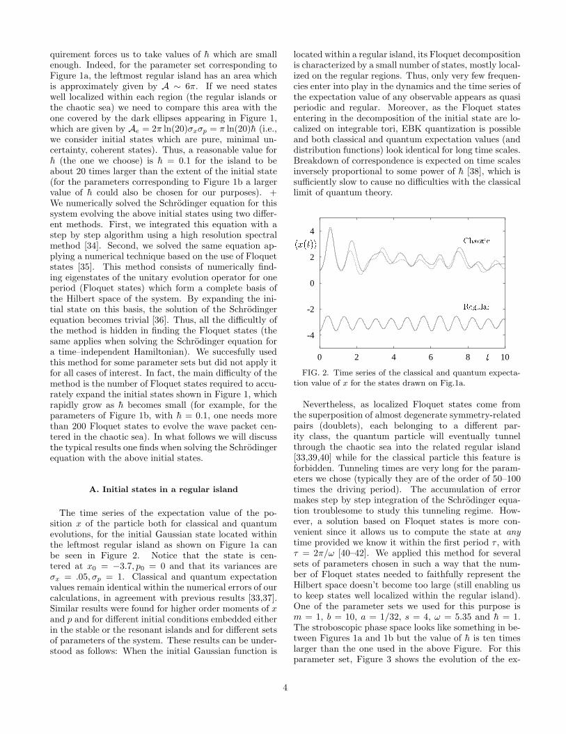
The time series of the expectation value of the po-sition x of the particle both for classical and quantumevolutions, for the initial Gaussian state located withinthe leftmost regular island as shown on Figure 1a canbe seen in Figure 2. Notice that the state is cen-tered at x0 = −3.7, p0 = 0 and that its variances areσx = .05, σp = 1. Classical and quantum expectationvalues remain identical within the numerical errors of ourcalculations, in agreement with previous results [33,37].Similar results were found for higher order moments of xand p and for different initial conditions embedded eitherin the stable or the resonant islands and for different setsof parameters of the system. These results can be under-stood as follows: When the initial Gaussian function is

located within a regular island, its Floquet decompositionis characterized by a small number of states, mostly local-ized on the regular regions. Thus, only very few frequen-cies enter into play in the dynamics and the time series ofthe expectation value of any observable appears as quasiperiodic and regular. Moreover, as the Floquet statesentering in the decomposition of the initial state are lo-calized on integrable tori, EBK quantization is possibleand both classical and quantum expectation values (anddistribution functions) look identical for long time scales.Breakdown of correspondence is expected on time scalesinversely proportional to some power of h [38], which issufficiently slow to cause no difficulties with the classicallimit of quantum theory.

RegularChaoti

t

hx(t)i-4

-2

0

2

4

0 2 4 6 8 10

FIG. 2. Time series of the classical and quantum expecta-tion value of x for the states drawn on Fig.1a.

Nevertheless, as localized Floquet states come fromthe superposition of almost degenerate symmetry-relatedpairs (doublets), each belonging to a different par-ity class, the quantum particle will eventually tunnelthrough the chaotic sea into the related regular island[33,39,40] while for the classical particle this feature isforbidden. Tunneling times are very long for the param-eters we chose (typically they are of the order of 50–100times the driving period). The accumulation of errormakes step by step integration of the Schrodinger equa-tion troublesome to study this tunneling regime. How-ever, a solution based on Floquet states is more con-venient since it allows us to compute the state at any

time provided we know it within the first period τ , withτ = 2π/ω [40–42]. We applied this method for severalsets of parameters chosen in such a way that the num-ber of Floquet states needed to faithfully represent theHilbert space doesn’t become too large (still enabling usto keep states well localized within the regular island).One of the parameter sets we used for this purpose ism = 1, b = 10, a = 1/32, s = 4, ω = 5.35 and h = 1.The stroboscopic phase space looks like something in be-tween Figures 1a and 1b but the value of h is ten timeslarger than the one used in the above Figure. For thisparameter set, Figure 3 shows the evolution of the ex-

4

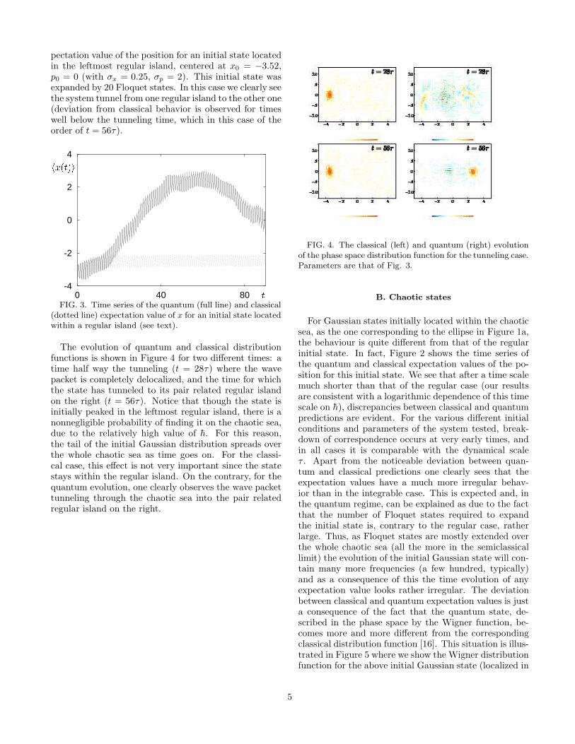
pectation value of the position for an initial state locatedin the leftmost regular island, centered at x0 = −3.52,p0 = 0 (with σx = 0.25, σp = 2). This initial state wasexpanded by 20 Floquet states. In this case we clearly seethe system tunnel from one regular island to the other one(deviation from classical behavior is observed for timeswell below the tunneling time, which in this case of theorder of t = 56τ).

t

hx(t)i

-4

-2

0

2

4

0 40 80FIG. 3. Time series of the quantum (full line) and classical

(dotted line) expectation value of x for an initial state locatedwithin a regular island (see text).

The evolution of quantum and classical distributionfunctions is shown in Figure 4 for two different times: atime half way the tunneling (t = 28τ) where the wavepacket is completely delocalized, and the time for whichthe state has tunneled to its pair related regular islandon the right (t = 56τ). Notice that though the state isinitially peaked in the leftmost regular island, there is anonnegligible probability of finding it on the chaotic sea,due to the relatively high value of h. For this reason,the tail of the initial Gaussian distribution spreads overthe whole chaotic sea as time goes on. For the classi-cal case, this effect is not very important since the statestays within the regular island. On the contrary, for thequantum evolution, one clearly observes the wave packettunneling through the chaotic sea into the pair relatedregular island on the right.

FIG. 4. The classical (left) and quantum (right) evolutionof the phase space distribution function for the tunneling case.Parameters are that of Fig. 3.

B. Chaotic states

For Gaussian states initially located within the chaoticsea, as the one corresponding to the ellipse in Figure 1a,the behaviour is quite different from that of the regularinitial state. In fact, Figure 2 shows the time series ofthe quantum and classical expectation values of the po-sition for this initial state. We see that after a time scalemuch shorter than that of the regular case (our resultsare consistent with a logarithmic dependence of this timescale on h), discrepancies between classical and quantumpredictions are evident. For the various different initialconditions and parameters of the system tested, break-down of correspondence occurs at very early times, andin all cases it is comparable with the dynamical scaleτ . Apart from the noticeable deviation between quan-tum and classical predictions one clearly sees that theexpectation values have a much more irregular behav-ior than in the integrable case. This is expected and, inthe quantum regime, can be explained as due to the factthat the number of Floquet states required to expandthe initial state is, contrary to the regular case, ratherlarge. Thus, as Floquet states are mostly extended overthe whole chaotic sea (all the more in the semiclassicallimit) the evolution of the initial Gaussian state will con-tain many more frequencies (a few hundred, typically)and as a consequence of this the time evolution of anyexpectation value looks rather irregular. The deviationbetween classical and quantum expectation values is justa consequence of the fact that the quantum state, de-scribed in the phase space by the Wigner function, be-comes more and more different from the correspondingclassical distribution function [16]. This situation is illus-trated in Figure 5 where we show the Wigner distributionfunction for the above initial Gaussian state (localized in

5

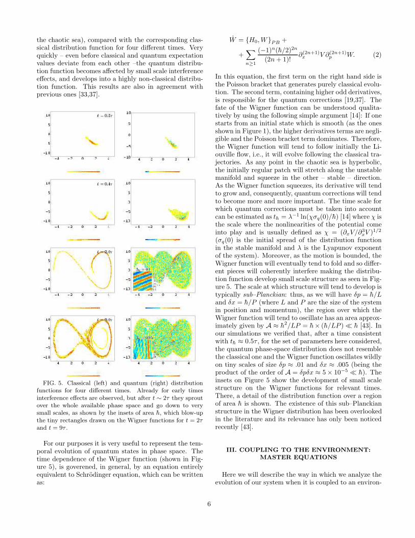
the chaotic sea), compared with the corresponding clas-sical distribution function for four different times. Veryquickly – even before classical and quantum expectationvalues deviate from each other –the quantum distribu-tion function becomes affected by small scale interferenceeffects, and develops into a highly non-classical distribu-tion function. This results are also in agreement withprevious ones [33,37].

FIG. 5. Classical (left) and quantum (right) distributionfunctions for four different times. Already for early timesinterference effects are observed, but after t ∼ 2τ they sproutover the whole available phase space and go down to verysmall scales, as shown by the insets of area h, which blow-upthe tiny rectangles drawn on the Wigner functions for t = 2τand t = 9τ .

For our purposes it is very useful to represent the tem-poral evolution of quantum states in phase space. Thetime dependence of the Wigner function (shown in Fig-ure 5), is goverened, in general, by an equation entirelyequivalent to Schrodinger equation, which can be writtenas:

W = H0,WPB +

+∑

n≥1

(−1)n(h/2)2n

(2n+ 1)!∂(2n+1)

x V ∂(2n+1)p W. (2)

In this equation, the first term on the right hand side isthe Poisson bracket that generates purely classical evolu-tion. The second term, containing higher odd derivatives,is responsible for the quantum corrections [19,37]. Thefate of the Wigner function can be understood qualita-tively by using the following simple argument [14]: If onestarts from an initial state which is smooth (as the onesshown in Figure 1), the higher derivatives terms are negli-gible and the Poisson bracket term dominates. Therefore,the Wigner function will tend to follow initially the Li-ouville flow, i.e., it will evolve following the classical tra-jectories. As any point in the chaotic sea is hyperbolic,the initially regular patch will stretch along the unstablemanifold and squeeze in the other – stable – direction.As the Wigner function squeezes, its derivative will tendto grow and, consequently, quantum corrections will tendto become more and more important. The time scale forwhich quantum corrections must be taken into accountcan be estimated as th = λ−1 ln(χσq(0)/h) [14] where χ isthe scale where the nonlinearities of the potential comeinto play and is usually defined as χ = (∂xV/∂

3xV )1/2

(σq(0) is the initial spread of the distribution functionin the stable manifold and λ is the Lyapunov exponentof the system). Moreover, as the motion is bounded, theWigner function will eventually tend to fold and so differ-ent pieces will coherently interfere making the distribu-tion function develop small scale structure as seen in Fig-ure 5. The scale at which structure will tend to develop istypically sub–Planckian: thus, as we will have δp = h/Land δx = h/P (where L and P are the size of the systemin position and momentum), the region over which theWigner function will tend to oscillate has an area approx-imately given by A ≈ h2/LP = h× (h/LP ) ≪ h [43]. Inour simulations we verified that, after a time consistentwith th ≈ 0.5τ , for the set of parameters here considered,the quantum phase-space distribution does not resemblethe classical one and the Wigner function oscillates wildlyon tiny scales of size δp ≈ .01 and δx ≈ .005 (being theproduct of the order of A = δpδx ≈ 5 × 10−5 ≪ h). Theinsets on Figure 5 show the development of small scalestructure on the Wigner functions for relevant times.There, a detail of the distribution function over a regionof area h is shown. The existence of this sub–Planckianstructure in the Wigner distribution has been overlookedin the literature and its relevance has only been noticedrecently [43].

III. COUPLING TO THE ENVIRONMENT:

MASTER EQUATIONS

Here we will describe the way in which we analyze theevolution of our system when it is coupled to an environ-

6

ment. The role of such environment will be played in ourcase by an infinite number of oscillators coupled to thesystem via an interaction term in the Hamiltonian, whichis assumed to be bilinear both in the coordinates of thesystem and the oscillators. As we are interested in follow-ing the evolution of the system solely, we will compute thereduced density matrix ρ obtained from the full densitymatrix of the Universe (system+environment) by tak-ing the partial trace over the environment ρ = TrE(ρU ),where ρU is the full density matrix of the Universe. Thisreduced density matrix will obey a master equation whichcan be obtained from the full von–Neumann equation bytracing out the environment. There is a vast literaturedealing with the properties of the master equation ob-tained under a variety of assumptions. Our purpose hereis not to present a review of these results but to sketchthe basic method used to obtain the master equationswe will use for our studies below (see [10] for a more ex-tensive review on the derivation and properties of masterequations in studies of decoherence).

The general approach to obtain the master equationis the following: We model the environment by a set ofharmonic oscillators with mass mi and natural frequencyωi, in thermal equilibrium at temperature T. The Hamil-

tonian is HR =∑

i ωi (b†ibi + 1/2), where bi and b†i arethe annihilation and creation operators, respectively, fora boson mode of frequency ωi. We further assume thatthe interaction Hamiltonian between the system and the

environment is HI = x∑

i(gi bi + g∗i b†i ), where gi are

coupling constants.The evolution of the reduced density matrix of the par-

ticle can be obtained by taking the partial trace over theenvironment of the exact von Neumann equation for thefull Hamiltonian, that reads i h ˙ρU = [ H(t) , ρU]. This canbe straightforwardly done under a number of standardassumptions (see [10] for more details): First, one as-sumes that the system and the environment are initiallyuncorrelated and that the reservoir is in an initial state ofthermal equilibrium at some temperature T . Second, oneassumes that the system and the environment are veryweakly coupled. So, solving the von Neumann equationperturbatively in the interaction picture (up to secondorder in perturbation theory) a master equation for thereduced density operator is obtained, which fully deter-mines the quantum dynamics of our system. It reads:

ρ(t) = −∫ t

0

dt′ gS(t− t′) [x(t) , [x(t′) , ρ(t) ] ] +

+ ı

∫ t

0

dt′ gA(t− t′) [x(t) , x(t′) , ρ(t) ] , (3)

where the above kernels are

gS(t− t′) =∑

i

|gi|2(1 + 2n(ωi)) cos(ωi(t− t′)) ,

gA(t− t′) =∑

i

|gi|2 sin(ωi(t− t′)) , (4)

with n(ω) = 1eβhω−1

(and β = 1/kBT ). It is worth stress-ing that the above master equation is derived withoutappealing to the usual Markovian approximation (see[10,22]). However, in our studies we restrict ourselves tothe Markovian regime where the kernels (4) are local intime. We solved the above master equation for two differ-ent regimes and environmental couplings. First, we con-sidered the widely used ohmic–high temperature regimeof the Brownian motion model where a simple masterequation can be written and solved. Second, we obtaineda master equation for the evolution of a coarse graineddensity matrix obtained from eq. (3) by averaging overone driving period. This can be naturally done by usingthe Floquet representation and is useful to study someproperties of the open system in the long time regime.We will now describe the two methods.

A. Ohmic–high temperature environment

The simplest special case of equation (3) follows whenassuming the high temperature limit of an Ohmic envi-ronment. Defining an spectral density for the environ-ment as J(ω) = lim∆ω→0

π∆ω

∑

ω<ωi<ω+∆ω |gi|2, assum-

ing that the spectrum is ohmic, i.e., that J(ω) = γmω/h,and going to the high temperature limit, gS(t − t′) =

D δ(t−t′) and gA(t−t′) = 2γδ(t−t′) with D = 2mγkBT ,the following well known equation for the Wigner func-tion of the system is obtained:

W = H0,WPB +∑

n≥1

(−1)nh2n

22n(2n+ 1)!∂(2n+1)

x V ∂(2n+1)p W

+ 2γ∂p (pW ) +D∂2ppW. (5)

The physical effects included in this equation are wellunderstood: The first term on the right hand side is thePoisson bracket generating the classical evolution for theWigner distribution function W ; the terms in h add thequantum corrections. The environmental effects are con-tained in the last two terms generating, dissipation anddiffusion, respectively. In the high-T limit here consid-ered dissipation can be ignored and only the diffusivecontributions need be kept (doing this we are taking theγ → 0 limit while keeping D constant). The diffusionconstant was chosen small enough so that energy is nearlyconserved over the time scales of interest. Equation (5)was integrated by means of a high resolution spectral al-gorithm [34]. Results were stable against changes bothin the resolution of phase space and the time accuracyrequired on each integration step. They will be presentedon Section 4.

7

B. Coarse grained master equation in the Floquet

basis:

It is interesting to write equation (3) in the Floquetbasis |ψµ(t)〉 = exp−ıεµt |φµ(t)〉, where the |φµ(t)〉 are τ -periodic, taking advantage of the τ -symmetry of our sys-tem H0. There are in the literature several approachesof the kind [39–42]. Ours is similar to that of Kohleret. al. [44], though in that reference the authors haverestricted the use of the equation to the study of chaotictunneling near a quasienergy crossing. When one writesthe master equation in the Floquet basis and takes theMarkovian high temperature limit, the resulting equationhas τ–periodic coefficients. Therefore, one can derive atemporal coarse–grained equation by taking the averageof such equation over one oscillation period. The result-ing equation for the average density matrix in one periodσ turns out to be

σµ,ν =∑

α,β

Mµ,ν,α,βσα,β , (6)

where the coefficients Mµ,ν,α,β are defined as

Mµ,ν,α,β = − ı

h(εµ − εν) δα,µδβ,ν −D δβ,ν〈〈x2〉〉µ,α

+ δα,µ〈〈x2〉〉β,ν − 2 〈〈x〉〉µ,α 〈〈x〉〉β,ν (7)

where the notation 〈〈A〉〉µ,ν = 1τ

∫ t+τ

t dt′〈φµ(t′)|A|φν(t′)〉is used to denote time averages of matrix elements of op-erators in the Floquet basis. As this is an equation withconstant coefficients, once these coefficients are numeri-cally calculated, the solution is formally obtained for all

times as σµ,ν(t) =∑

α,β

(

eMt)

µ,ν,α,βσα,β(0). The diffi-

culty in solving this equation resides on the large numbern of Floquet states one typically needs to accurately rep-resent a state located in the chaotic sea (as we mentionedabove, a semiclassical argument to estimate the numberof such states is given by the ratio A/(2πh), where Ais the area of the chaotic sea, which might quickly be-come a very large number). As M has dimension n4,numerical limitations spring up at this point. However,for some parameter values it was still possible to managethe numerical problem. The results will be presented onSection V.

IV. RESULTS

Before going into a detailed description of our modelfor the open system it is instructive to analyze equation(5) so as to have an intuitive idea of what is going on.When the diffusion term is absent –that means, statesevolve simply according to Schrodinger equation– for asmooth initial state the dominant term is the Poissonbracket. As we already discussed in Section 2, the Wignerfunction initially evolves following nonlinear classical tra-jectories, looses its Gaussian shape and develops tendrils

while folding. If the initial state is located in the chaoticsea, this happens exponentially fast. Due to the combi-nation of squeezing-stretching and folding the gradientsincrease and quantum corrections in equation (5) becomeimportant, so discrepancies between quantum and clas-sical predictions begin to be relevant. Also, quantuminterferences among different pieces of the wave packetdevelop and generate oscillations in the Wigner function.

The effect of the decoherence producing term in equa-tion (5) can be understood as being responsible of twointerrelated effects: On the one hand, the diffusion termtends to wash out the oscillations in the Wigner functionsuppressing quantum interferences. Thus, for this systemdecoherence is the dynamical suppression of the interfer-ence fringes that are dynamically produced by nonlinear-ities. The time–scale characterizing the disappearance ofthe fringes can be estimated easily using previous results[6]: Fringes with a characteristic wave vector (along thep–axis of phase space) kp decay exponentially with a rategiven by ΓD = Dk2

p. Noting that a wave packet spreadover a distance ∆x with two coherently interfering piecesgenerate fringes with kp = ∆x/h one concludes that the

decoherence rate is ΓD = D∆2x/h

2. This rate dependslinearly on the diffusion constant. When the Wignerfunction is coherently spread over the whole availablephase space one expects fringes with wavelength of theorder of 1/L where L is the size of the system (these areresponsible for the existence of sub–Planck structure inthe Wigner function, as mentioned in Section 2). Therate at which these fringes disappear due to decoherenceis then ΓD = DL2/h2. Thus, we can derive a conditionthat should be satisfied in order for these fringes to be ef-ficiently destroyed by decoherence: the destruction of thefringes, that takes place at a rate ΓD, should be fasterthan their regeneration, that takes place at a rate Ωf

fixed by the system’s dynamics and related both to theLyapunov time and the folding rate. Thus, if Ωf ≪ ΓD

the small scale fringes will be efficiently washed out andthe Wigner function would remain essentially positive. Itis worth mentioning that the destruction of fringes wouldgenerate entropy at a rate which, provided the conditionΩf ≪ ΓD is satisfied, should be independent of the dif-fusion constant, and should be fixed by Ωf . Thus, onecould argue that every time the Wigner function stretchesand folds, becoming an approximate coherent superposi-tion of two approximately orthogonal states, the destruc-tion of the corresponding fringes should generate aboutone bit of entropy. If the timescale for the fringe disap-pearance (ΓD) is much smaller than the one for producingthe above superposition (fixed by Ωf ) then the entropyproduction rate would be simply equal to Ωf (ideally,one would expect one bit of entropy created after a time1/Ωf).

However, the disappearance of the interference fringesis not the only effect produced by decoherence. Thereis a second related consequence of this process (whichis also present in the classical case): While interference

8

fringes are being washed out by decoherence, the dif-fusion term also tends to spread the regions where theWigner function is possitive, contributing in this way tothe entropy growth. But, as discussed in [14,28], the rateof entropy production distinguishes regular and chaoticcases. For regular states, decoherence should produce en-tropy at a rate which depends on the diffusion constantD. However, for chaotic states the rate should becomeindependent of D and should be fixed by the Lyapunovexponent. The origin of this D-independent phase can beunderstood using a simple minded argument (presentedfirst in [14] and later discussed in a more elaborated wayin [28]): Chaotic dynamics tends to contract the Wignerfunction along some directions in phase space competingagainst diffusion. These two effects balance each othergiving rise to a critical width below which the Wignerfunction cannot contract. This local width should beapproximately σ2

c = 2D/λ (being λ the local Lyapunovexponent). Once the critical size has been reached, thecontraction stops along the stable direction while the ex-pansion continues along the unstable one. Therefore,in this regime the area covered by the Wigner functiongrows exponentially in time and, as a consequence, en-tropy grows linearly with a rate fixed by the Lyapunovexponent. Moreover, the appearance of a lower boundfor the squeezing of the Wigner function make quantumcorrections unimportant and so the Wigner function willevolve classically (following Liouville flow plus diffusiveeffects), and the correspondence will be reestablished.

In this Section we present solid numerical evidence sup-porting the existence of this D-independent phase. Forsimplicity, instead of looking at the von Neumann en-tropy HV N = −Tr (ρr log ρr) we examine the linear en-tropy, defined as H = − log(Tr

(

ρ2r

)

), which is a goodmeasure of the degree of mixing of the system and sets alower bound on HV N (i.e, one can show that HV N ≥ H).The above argument concerning the role of the criticalwidth σc may appear as too simple but captures the es-sential aspects of the dynamical process. We can presenta more elaborate argument using the master equation(5) to show that the rate of linear entropy productioncan always be written as:

H = 2D〈(∂pW )2〉/〈W 2〉, (8)

where the bracket denotes an integral over phase space.The right hand side of this equation is proportional to themean square wave–number computed with the square ofthe Fourier transform of the Wigner function. This im-plies that the entropy production rate is closely related tothe phase space structure present in the Wigner distribu-tion. Thus, the D–independent phase begins at the timewhen the mean square wave–length along the momentumaxis scales with diffusion as

√D (as σc does). This behav-

ior cancels the diffusion dependence of H which becomesentirely determined by the dynamics.

Appart from analyzing theD–independent phase of en-tropy production we analyze the nature of the the tran-sition between the diffusion dominated to the chaotic

regime. This time tc can also be estimated along thelines of the previous argument: The time for which thespread of the Wigner function approches the critical oneis tc ≈ λ−1 log(σp(0)/σc). According to this estimatetc should depend logarithmically on the diffusion con-stant and on the initial spread of the Wigner function(for Gaussian initial states the spread depends exponen-tially on the initial entropy, therefore tc should vary asa linear function of the initial entropy). Our numericalwork is devoted to testing these intuitive ideas.

In the following subsections we present our results.First, we will show (for completeness of our presenta-tion) how decoherence restores classicality washing outinterference fringes. Then, we focus on our main goal:the study of the entropy production rate of the systemas a function of time.

A. Correspondence principle restored:

disappearance of interference fringes

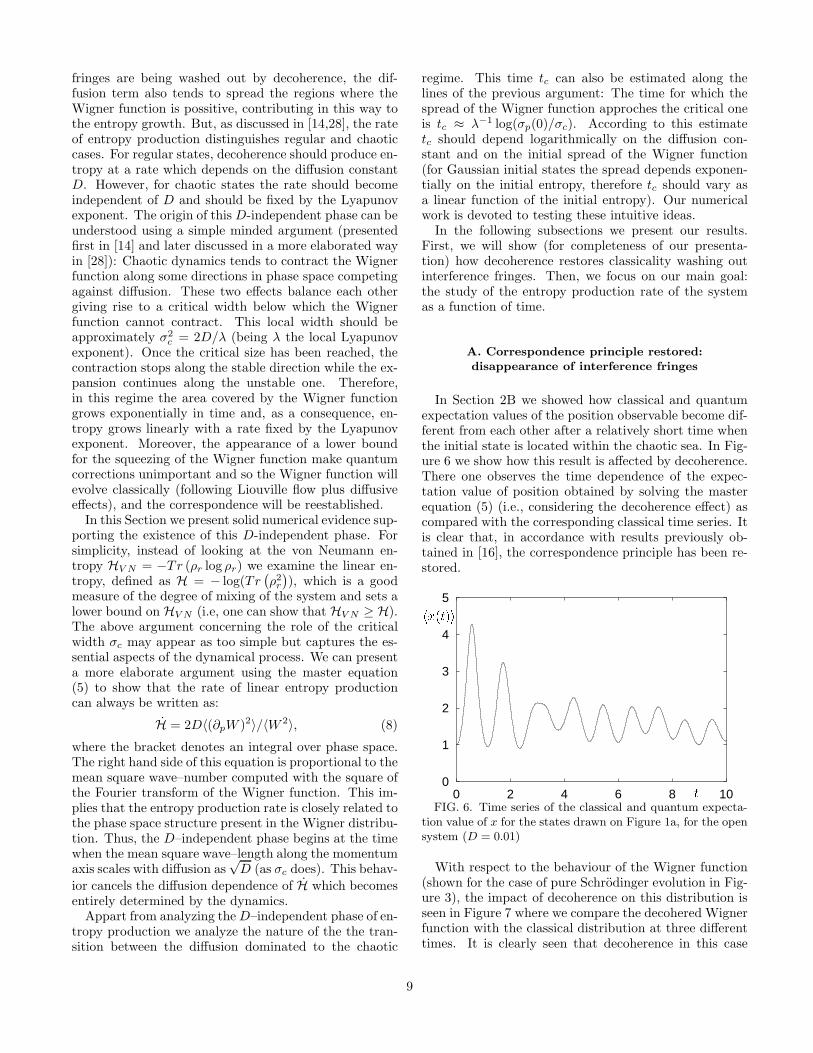
In Section 2B we showed how classical and quantumexpectation values of the position observable become dif-ferent from each other after a relatively short time whenthe initial state is located within the chaotic sea. In Fig-ure 6 we show how this result is affected by decoherence.There one observes the time dependence of the expec-tation value of position obtained by solving the masterequation (5) (i.e., considering the decoherence effect) ascompared with the corresponding classical time series. Itis clear that, in accordance with results previously ob-tained in [16], the correspondence principle has been re-stored.

t

hx(t)i

0

1

2

3

4

5

0 2 4 6 8 10FIG. 6. Time series of the classical and quantum expecta-

tion value of x for the states drawn on Figure 1a, for the opensystem (D = 0.01)

With respect to the behaviour of the Wigner function(shown for the case of pure Schrodinger evolution in Fig-ure 3), the impact of decoherence on this distribution isseen in Figure 7 where we compare the decohered Wignerfunction with the classical distribution at three differenttimes. It is clearly seen that decoherence in this case

9

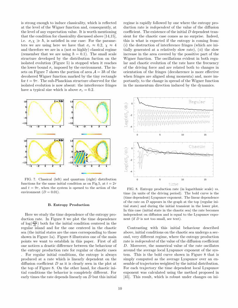
is strong enough to induce classicality, which is reflectedat the level of the Wigner function and, consequently, atthe level of any expectation value. It is worth mentioningthat the condition for classicality discussed above [14,15],i.e. σcχ ≫ h, is satisfied in our case: For the parame-ters we are using here we have that σc ≈ 0.2, χ ≈ 4and therefore we are in a (not so highly) classical regime(remember that we are using h = 0.1). The small scalestructure developed by the distribution fuction on theisolated evolution (Figure 5) is stopped when it reachesthe lower bound σc imposed by the environment. The in-sets on Figure 7 shows the portion of area A = 3h of thedecohered Wigner function marked by the tiny rectanglefor t = 9τ . The sub-Planckian structure observed for theisolated evolution is now absent: the interference fringeshave a typical size which is above σc = 0.2.

FIG. 7. Classical (left) and quantum (right) distributionfunctions for the same initial condition as on Fig.5, at t = 2τand t = 9τ , when the system is opened to the action of theenvironment (D = 0.01).

B. Entropy Production

Here we study the time dependence of the entropy pro-duction rate. In Figure 8 we plot the time dependenceof log(dH

dt ) both for the initial condition centered in theregular island and for the one centered in the chaoticsea (the initial states are the ones corresponding to thoseshown in Figure 1a). Figure 8 illustrates one of the mainpoints we want to establish in this paper. First of allone notices a drastic difference between the behaviour ofthe entropy production rate for regular or chaotic cases. For regular initial conditions, the entropy is alwaysproduced at a rate which is linearly dependent on thediffusion coefficient D as it is clearly seen in the plot atthe top of Figure 8. On the other hand, for chaotic ini-tial conditions the behavior is completely different. Forearly times the rate depends linearly on D but this initial

regime is rapidly followed by one where the entropy pro-duction rate is independent of the value of the diffusioncoefficient. The existence of the initialD dependent tran-sient for the chaotic case comes as no surprise. Indeed,this is what is expected if the entropy is coming from:(i) the destruction of interference fringes (which are ini-tially generated at a relatively slow rate), (ii) the slowincrease in the area covered by the possitive part of theWigner function. The oscillations evident in both regu-lar and chaotic evolution of the rate have the frecuencyof the driving force and are related both to changes inorientation of the fringes (decoherence is more effectivewhen fringes are aligned along momenta) and, more im-portantly, to the change in spread of the Wigner functionin the momentum direction induced by the dynamics.

0 5 10 15

-4

-2

0

0 5 10 15

-4

-2

0

FIG. 8. Entropy production rate (in logarithmic scale) vs.

time (in units of the driving period). The bold curve is the(time dependent) Lyapunov exponent. The linear dependenceof the rate on D appears in the graph at the top (regular ini-tial state) and during the initial transient in the lower plot.In this case (initial state in the chaotic sea) the rate becomesindependent on diffusion and is equal to the Lyapunov expo-nent (if D is not too small, see text).

Contrasting with this initial behaviour describedabove, initial conditions on the chaotic sea undergo a sec-ond, very different regime, where the entropy productionrate is independent of the value of the diffusion coefficientD. Moreover, the numerical value of the rate oscillatesaround the average local Lyapunov exponent of the sys-tem. This is the bold curve shown in Figure 8 that issimply computed as the average Lyapunov over an en-semble of trajectories weighted by the initial distribution.For each trajectory the time dependent local Lyapunovexponent was calculated using the method proposed in[45]. This result, which is robust under changes on ini-

10

tial conditions and on the parameters characterizing thedynamics, confirms the conjecture first presented in [14].

It is interesting to remark that while the simple pic-ture presented in [14] is in good qualitative agreementwith our results, the arguments presented in that pa-per are too simple to include some important effects wefound here. In particular the oscillatory nature of therate was completely overlooked in [14]. However, havingsaid this, it is still possible to test some important re-sults obtained in [14] for the transition time tc betweenboth regimes. First, we analyzed the dependence of thetransition time on the diffusion coefficient D. Due to theoscillatory nature of the rate, there is some ambiguityin the definition of tc. Here, we defined it as the timefor which the rate reaches some value after the initialtransient. As the rate goes through a jump of two or-ders of magnitude when changing from one regime to theother, this definition is a reasonable one. Thus, we founda logarithmic dependence of the transition time on thediffusion coefficient, as can be seen on Figure 9. Second,we investigated the behaviour of the rate as a functionof the entropy of the initial state. Our definition of tc isthe same as before. Parameters of the system for thesestudies where those that would allow states with initialentropy up to H(0) = 4 be easily located within thechaotic sea. We obtained thus the results shown on Fig-ure 9, where a linear dependence of the transition timetc on H(0) is clearly seen. Both results confirm the naiveexpectation concerning the nature of tc that we discussedabove.

It is remarkable that for long times the entropy produc-tion rate is indeed fixed just by the dynamics, becomingindependent of D (after all, the entropy production isitself a consecuence of the coupling to the environmentbut the value of the rate becomes independent of it!).The results presented in Figures 8 and 9 were shown tobe robust under changes of initial conditions and otherparameters characterizing the classical dynamics.

2 2.5 3 3.51

1.1

1.2

1.3

1.4

0 1 2 3 4

1.4

1.6

1.8

2

FIG. 9. The transition time between the diffusion domi-nated regime and the one where the entropy production rateis set by the Lyapunov exponent is shown to depend linearlyon entropy (top) and logarithmically on the diffusion constant(bottom). Numerical results were obtained using the param-eters: B = 10, C = 0.5, E = 10, ω = 6.16, D = 10−3 (top),H(0) = 0 (bottom)

There are two limitations for the above results to beobtained. On the one hand the diffusion constant cannotbe too strong: In that case the system heats up too fastand the entropy saturates, making the numerical simula-tions unreliable. On the other hand, diffusion cannot betoo small either: If that is the case decoherence may be-come too weak and the interference fringes could persistover many oscillations; the minimal value of D requiredfor efficient decoherence could be estimated as describedabove: If the Wigner function is coherently spread over aregion of size ∆x ∼ L, we would need a diffusion constantlarger thanDmin ≈ h2/L2 ∼ 10−4 for the environment tobe able to wash out the smallest fringes in one driving pe-riod (this is nothing but the above condition Ωf ≪ ΓD).In fact, Figure 8 shows that when D = 10−5 the entropyproduction rate is one order of magnitude smaller thanthe one corresponding to D = 10−4. Thus, for values ofD that are too small,the condition for classicality is not

satisfied and the D independent phase of the evolutionis never attained: the Wigner function always retain asignificant negative part and decoherence is not effective.

V. DECOHERENCE AND THE SUPPRESSION

OF TUNNELLING

For initial states localized in the regular islands corre-spondence is broken for long times when tunnelling be-comes effective, as pointed in Section 2A. Here, we in-

11

vestigate the influence of decoherence on this process byusing our coarsed-grained master equation (6). In doingthis we should be carefull to choose a number of Flo-quet states which is large enough. Thus, decoherencecouples these states and the expected quasi–equilibriumstate one gets from the master equation should be ap-proximately diagonal in the Floquet basis. One expectsthat using n Floquet states to expand our Hilbert space,the master equation would tend to mix the state in sucha way that the entropy would grow up to a level where allstates become occupied with equal probability. At thispoint the numerical simulation done in this way becomesclearly unreliable. We solved the master equation com-puting the Von Neumann entropy HV N = −Tr(σ log σ)checking that its value is kept well below saturation. Forthe same parameters we described in Section 2A (and us-ing Floquet 40 states instead) we were able to accuratelystudy the tunnelling process from an initial state local-ized in the leftmost regular island. We analized the evo-lution of the expectation value of position 〈x〉 = Tr[xσ]which is shown in Figure 11. Suppression of tunnelingis clearly observed. Notice that the asymptotic value xa

of 〈x〉, though small, is not zero. This value can be es-timated as xa = limt→∞

∫

(x,p)⊆Ω dxdpxW (x, p, t) where

Ω is the region of the phase space within the leftmostregular island where the state is initially located. Thenumerical result shown in the above Figure is consistentwith this estimate, meaning that the final state σ has asignificant part which remains trapped in the left of thewell. The evolution of the Wigner distribution function,shown on Figure 10 for t = 28τ and t = 56τ , illustratesthe described behaviour of the state of the system. It isalso noticeable that the state is trapped in the leftmostisland as a result of the interaction with the environment.

FIG. 10. Classical (left) and quantum (right) evolution ofthe Gaussian state initially localized at the leftmost regularisland (see Section 2A) when the system is opened to theaction of the environment environment (D = 0.01), for thetunneling case.

t

hx(t)i

-4

-2

0

2

4

0 40 80

FIG. 11. Time series of the quantum expectation value ofx for the state of Fig.3

It is interesting to notice that this picture would dras-tically change if the coupling to the environment isswitched on at a time t0 > 0 (i.e., if we let the sys-tem to evolve freely, with its own Hamiltonian, beforecoupling it to the environment). This is very easy to dousing the above master equation. The results obtainedin this way are simple and intuitive: If we switch on thecoupling to the environment at a time when the systemhas already tunneled to the pair related island on theright (t = 56τ), the environment will simply stop thestate from tunnelling back to the initial island. Figure12 (right) shows the evolution of the Wigner function inthis case. Contrariwise, if we turn on the coupling tothe environment when the state is half way through thetunnelling (in an intermediate, delocalized, state at timet0 = 28τ), decoherence yields an asymptotic state whichhas approximately half of the probability in each side ofthe well (this is seen on the left column of Figure 12).

FIG. 12. Evolution of the Gaussian state initially localizedat the leftmost regular island (see Section 2A) when the en-vironment (D = 0.01) is connected at t0 = 28τ (on the left)or at t0 = 56τ (on the right).

12

VI. CONCLUSION

Quantum open systems become entangled with the en-vironments as a consequence of their interaction. For thisreason, information initially stored in the state of thesystem irreversibly leaks into the environment. The re-sults we presented here support the point of view stating[14] that for classically chaotic systems the rate at whichinformation flows from the system to the environment(the rate of von Neuman entropy production) is indepen-dent of the strength of the coupling to the environment(provided the coupling strength is above some threshold).Thus, our results show that for chaotic quantum systems,the classical limit enforced by environment induced deco-herence is quite different from the one corresponding toregular systems. Thus, we showed that this limit exhibitsan unavoidable source of unpredictability, being the rateat which information is lost into the environment entirelyfixed by the chaotic nature of the Hamiltonian of thesystem. To the contrary, for regular systems the entropyproduction rate is proportional to the strength of the cou-pling to the environment. Therefore, the existence of thisphase of coupling–independent entropy production couldbe used as a diagnostic for quantum chaos. Our resultsalso confirm previous estimations [14,17] for the transi-tion time tc between the two regimes: the one where theentropy production rate is diffusion-dominated and theone set by the chaotic dynamics, that is, a linear depen-dence of tc on the initial entropy (initial spread) and alogarithmic dependence on the diffusion constant.

From our results it is possible to develop an intuitivepicture for the reason why entropy production rate be-comes dominated by the chaotic dynamic. As we de-scribed in the paper, there are two interrelated processescontributing to the growth of entropy. First, the destruc-tion of the interference fringes which are dynamicallyproduced in phase space by the streaching and foldingof the chaotic evolution. The entropy production rateassociated with this process is obviously determined bythe slowest of the two timescales corresponding to theproceses of creation and anihillation of fringes. There-fore, when decoherence is effective, and the fringes diss-appear in a short timescale, the entropy production rateis of dynamical origin (and independent of the couplingstrength between the system and the environment). Onthe other hand the spread of the possitive peaks of theWigner function also contributes to the entropy growth.In this case, the rate becomes independent of the couplingstrength once the phase space distribution approaches acritical width. Both of these processes are present in ageneral case (only it is possible to study them separatelyin idealized cases such as in the baker’s map [46]). Theresults of this paper confirm this intuitive view, whichcan be made more precise when formulated in terms ofequation (8).

This work was partially supported by Ubacyt (TW23),Anpcyt, Conicet and Fundacion Antorchas. JPP thanks

W. Zurek for many useful discussions and hospitality dur-ing his visits to Los Alamos.

[1] Zurek, W. H., Physics Today 44, 36 (1991).[2] Giulini, D., Joos, E., Kiefer, C., Kupsch, J., Stamatescu,

I.-O., and Zeh, H. D., Decoherence and the Appearance of

a Classical World in Quantum Theory, (Springer, Berlin,1996).

[3] Zurek, W. H., Phys. Rev. D 24, 1516-1524 (1981).[4] Zurek, W. H., Phys. Rev. D 26, 1862-1880 (1982).[5] Zurek, W. H., pp. 145-149 in Frontiers of Non-

equilibrium Statistical Mechanics, G. T. Moore and M.O. Scully, eds. (Plenum, New York, 1986).

[6] Paz, J. P., Habib, S., and Zurek, W. H., Phys. Rev. D

47, 488 (1993).[7] Zurek, W. H., Progr. Theor. Phys. 89, 281-302 (1993).[8] Zurek, W. H., Habib, S., and Paz, J. P., Phys. Rev. Lett.,

70, 1187, (1993).[9] Paz, J. P. and Zurek, W. H., Phys. Rev. Lett. 82, 5181

(1999).[10] Paz, J. P. and Zurek, W. H., quant-ph/0010011, to ap-

pear in the “Proceedings of the 72nd. Les Houches Sum-mer School”, Springer Verlag (2001), in press.

[11] Brune, M., Hagley, E., Dreyer, J., Maitre, X., Maali, A.,Wunderlich, C., Raimond, J-M., and Haroche, S., Phys.

Rev. Lett. 77, 4887-4890 (1996).[12] Cheng, C. C., and Raymer, M. G., Phys. Rev. Lett, 82,

4802 (1999)[13] Myatt, C. J., et al., Nature, 403, 269 (2000).[14] Zurek, W. H., and Paz, J. P., Phys. Rev. Lett. 72, 2508-

2511 (1994); ibid. 75, 351 (1995).[15] Zurek, W. H. and Paz, J. P., Physica D83, 300 (1995).[16] Habib, S., Shizume, K., and Zurek, W. H., Phys. Rev.

Lett, 80, 4361 (1998).[17] Monteoliva, D., and Paz, J. P., Phys. Rev. Lett. 87 (2000)

3373.[18] Wisdom, J., Peale, S. J., and Maignard, F. Icarus 58,

137 (1984); see also Wisdom, J., Icarus 63, 272 (1985);Laskar, J., Nature 338, 237 (1989); Sussman, G. J., andWisdom, J., Science 257, 56-62 (1992).

[19] Wigner, E. P., Phys. Rev. 40, 749 (1932). For a review,see Hillery, M., O’Connell, R. F., Scully, M. O., andWigner, E. P., Phys. Rep. 106, 121 (1984).

[20] Zurek, W. H., Physica Scripta T76, 186 (1998), alsoavailable at quant-ph/9802054.

[21] Karkuszewski Z., Zakrezewski J. and Zurek, W. H.Breakdown of correspondence in chaotic systems: Ehren-

fest versus localization times, preprint available atnlin.CD/0012048.

[22] Hu, B. L., Paz, J. P., and Zhang, Y., Phys. Rev. D 45,2843 (1992).

[23] Caldeira, A. O., and Leggett, A. J., Physica 121A, 587-616 (1983); Phys. Rev. A 31, 1059 (1985).

[24] Unruh, W. G., and Zurek, W. H., Phys. Rev. D 40, 1071-1094 (1989).

13

[25] Shiokawa, K., and Hu, B. L., Phys. Rev E 52, 2497(1995).

[26] Miller, P. A., and Sarkar, S. Phys. Rev. E 58, 4217(1998); E 60, 1542 (1999).

[27] Jalabert R. and Pastawski, H., Phys. Rev. Lett. 86, 2490(2001) and references therein.

[28] Pattanayak, A. K., Phys. Rev. Lett. 83, 4526 (2000).[29] Graham R., Z. Phys. B59, 75 (1985); Graham R. and Tel

T., Z. Phys. B60, 127 (1985); Dittrich T. and GrahamR., Z. Phys. B62, 515 (1986).

[30] F. Haake, Quantum signatures of chaos, Springer Se-ries in Synergetics, edited by H. Haken, vol 54, Springer(Berlin, 1991).

[31] Dittrich T., Hanggi P., Ingold G.-L., Kramer B., ShonG. and Zwerger W., Quantum transport and dissipation,Wiley–VCH (1998).

[32] L. E. Reichl and W. Zheng, Phys. Rev. A 29 (1984) 2186.[33] W. A. Lin and L. E. Ballentine, Phys. Rev. A 45 (1992)

3637; Phys. Rev. Lett 65 (1990) 2927.[34] M. Feit J. Fleck Jr. and A. Steiger, J. Comp. Phys. 47

(1992) 412.[35] J. Shirley, Phys. Rev. A 138 B (1965) 979.[36] K. F. Milfeld and R. Wyatt, Phys. Rev. A 27 (1983) 72.[37] K Takahashi, Prog. Theor. Phys. Supp. bf 98 (1989) 109.[38] M. Berry and N. L. Balazs, J. Phys. A 12 (1979) 625.[39] R. Utermann, T. Dittrich and P. Hanggi, Phys. Rev. E

49 (1994) 273.[40] F. Grossmann, T. Dittrich, P. Jung and P. Hanggi, J.

Stat. Phys. 70 (1993) 229.[41] T. Dittrich, B. Oelschlagel and P. Hanggi, Europhys.

Lett. 22 (1993) 5.[42] R.Blumel, A.Buchleitner, R. Graham, L. Sirko, U. Smi-

lansky and H. Walther, Phys. Rev. A44 (1991) 4521.[43] Zurek, W. H. (2000) private communication.[44] P. Hanggi, S. Kohler and T. Dittrich, in Proc. 1999 LNP

547, edited by D. Regera et al; (1999) 125–157, SpringerVerlag (Berlin); S. Kohler, R. Utermann, P. Hanggi andT. Dittich, Phys. Rev. E58 (1998) 7219 (also quant-ph/9804041).

[45] S. Habib and R. Ryne, Phys. Rev. Lett 74 (1995) 70.[46] P. Bianucci, J.P. Paz and M. Saraceno, Decoherence for

classically chaotic quantum maps, (2001) to be published.

14