Supplementary data to Cross-species common regulatory network inference without requirement for prior gene affiliation Amin Moghaddas Gholami 1, 2 and Kurt Fellenberg 1 1 Chair of Proteomics and Bioanalytics, Center for Integrated Protein Sciences Munich (CIPSM), Technische Universität München, Emil Erlenmeyer Forum 5, 85354 Freising, Germany. 2 Functional Genome Analysis, German Cancer Research Center (DKFZ), Im Neuenheimer Feld 580, 69120 Heidelberg, Germany. S1. Datasets and preprocessing The pair of normalized yeast microarray gene expression datasets described in the results section of the main text (Sce/Spo) was downloaded from the publically accessible ArrayExpress data repository (Cipollina et al., 2008b; Parkinson et al., 2009) as well as from the authors‟ web resource. After log2- transformation, genes for which more than 50% of the data were missing were discarded. The remaining missing values were imputed by k-nearest neighbor algorithm (Troyanskaya et al., 2001) and Spline interpolation (Bar-Joseph et al., 2003) which are commonly used for time-series data. Periodically expressed genes of significance with false discovery rate (FDR) of 0.05 were extracted by AR(1)-based background model (Futschik and Herzel, 2008). The second two datasets (human/mouse) were downloaded from Gene Expression Omnibus (Barrett et al., 2009). The studies investigated the effect of Estradiol on human (Stossi et al., 2004) and murine cells (Moggs et al., 2004). Stossi et al., examined U2OS osteosarcoma cells after treatment with either estrogen receptor (ER) alpha or beta for various periods of time up to 48 hours (10 time points in total). They generated U2OS human osteosarcoma cells stably expressing ESR1 or ESR2, at levels comparable to those in osteoblasts. The characterization of the response to estradiol (E2) over time is measured using Affymetrix GeneChip microarrays. Moggs and coworkers recorded the uterus response of immature mice subcutaneously injected with 17β-estradiol (E2) or arachis oil (AO) at various time points up to 72 hours following treatment. Datasets were normalized by variance stabilization (Huber et al., 2002). Differentially expressed genes were extracted using the eBayes method of the limma package (Smyth, 2004). For multiple testing adjustments, we calculated the FDR using the algorithm of Benjamini and Hochberg (Benjamini and Hochberg, 1995).

Welcome message from author
This document is posted to help you gain knowledge. Please leave a comment to let me know what you think about it! Share it to your friends and learn new things together.
Transcript

Supplementary data to
Cross-species common regulatory network inference
without requirement for prior gene affiliation
Amin Moghaddas Gholami1, 2
and Kurt Fellenberg1
1Chair of Proteomics and Bioanalytics, Center for Integrated Protein Sciences Munich (CIPSM), Technische Universität
München, Emil Erlenmeyer Forum 5, 85354 Freising, Germany. 2Functional Genome Analysis, German Cancer Research Center (DKFZ), Im Neuenheimer Feld 580, 69120 Heidelberg,
Germany.
S1. Datasets and preprocessing
The pair of normalized yeast microarray gene expression datasets described in the results section of the
main text (Sce/Spo) was downloaded from the publically accessible ArrayExpress data repository
(Cipollina et al., 2008b; Parkinson et al., 2009) as well as from the authors‟ web resource. After log2-
transformation, genes for which more than 50% of the data were missing were discarded. The remaining
missing values were imputed by k-nearest neighbor algorithm (Troyanskaya et al., 2001) and Spline
interpolation (Bar-Joseph et al., 2003) which are commonly used for time-series data. Periodically
expressed genes of significance with false discovery rate (FDR) of 0.05 were extracted by AR(1)-based
background model (Futschik and Herzel, 2008).
The second two datasets (human/mouse) were downloaded from Gene Expression Omnibus (Barrett et
al., 2009). The studies investigated the effect of Estradiol on human (Stossi et al., 2004) and murine
cells (Moggs et al., 2004). Stossi et al., examined U2OS osteosarcoma cells after treatment with either
estrogen receptor (ER) alpha or beta for various periods of time up to 48 hours (10 time points in total).
They generated U2OS human osteosarcoma cells stably expressing ESR1 or ESR2, at levels comparable
to those in osteoblasts. The characterization of the response to estradiol (E2) over time is measured using
Affymetrix GeneChip microarrays. Moggs and coworkers recorded the uterus response of immature
mice subcutaneously injected with 17β-estradiol (E2) or arachis oil (AO) at various time points up to 72
hours following treatment.
Datasets were normalized by variance stabilization (Huber et al., 2002). Differentially expressed genes
were extracted using the eBayes method of the limma package (Smyth, 2004). For multiple testing
adjustments, we calculated the FDR using the algorithm of Benjamini and Hochberg (Benjamini and
Hochberg, 1995).
S2. Co-inertia analysis and alternative methods
Integrating datasets into simultaneous analysis is a major challenge in systems biology. It is crucial to
capture the associations between variables from different high-throughput multidimensional datasets.
Different techniques exist to investigate the associations between large-scale datasets. Canonical
Correlation Analysis (CCA; (Gittins, 1985), Partial Least Square (PLS; (Wold, 1966) and Co-inertia
Analysis (CIA; (Dolédec and Chessel, 1994) transform high-dimensional data into few, usually two or
three dimensions for visualization.
PLS is a correlation based method. It explains relationships between two datasets by simultaneously
decomposing the data matrices into low-dimensional vectors. CCA is a special case of PLS, identifying
linear combinations of variables from each set such so that they have maximum correlation. However
CCA and PLS often suffer from the asymmetry of microarray datasets where the number of variables
exceeds the number of samples.
Penalized CCA adapted with Elastic Net (CCA-EN; (Cao et al., 2008; Waaijenborg et al., 2008) and
Sparse CCA (SCCA; (Parkhomenko et al., 2009) are derivatives of the classical CCA. They incorporate
variable selection to address above limitation of earlier approaches. However, if invoked repeatedly
from within an unsupervised iterative algorithm, it becomes computationally infeasible for large number
of variables.
In contrast, CIA can cope with both asymmetry and large number of variables without becoming
computationally infeasible. CIA is a multivariate coupling approach measuring the adequacy between
datasets. It was first introduced applying ecological data (Dolédec and Chessel, 1994), and amino acid
properties (Thioulouse and Lobry, 1995). Culhane and co-workers demonstrated the efficiency of CIA
on cross-platform comparisons of gene expression data, applying it to both cDNA and Affymetrix
microarrays (Culhane et al., 2003). An extension of CIA that links more than two tables has been
reported (Dray et al., 2003). Fagan and co-workers combined information from multiple layers (genes,
samples and GO terms) by CIA (Fagan et al., 2007).
In our algorithm we used CIA because of its visual interpretability, its speed and because its applicability
to asymmetric microarray data had been demonstrated in many studies (Culhane et al., 2003; Fagan et
al., 2007; Jeffery et al., 2007; Singh et al., 2007).

S2.1 Co-inertia definition
The mathematical basis of CIA, following the notation of Dolédec and coworkers (Culhane et al., 2003;
Dolédec and Chessel, 1994; Jeffery et al., 2007) is summarized as below.
Let X and Y be the original data tables, with n rows, and respectively p and q columns. The two
statistical triplets produced by the ordination methods performed on the datasets are denoted (X, Dn, Dp)
and (Y, Dn, Dq), with Dn and Dp being diagonal matrices containing row and column weights for X, and
Dn and Dq diagonal matrices containing row and column weights for Y. After diagonalization let u and v
be a pair of eigenvectors for (X, Dn, Dp) and (Y, Dn, Dq), respectively. The projection of the
multidimensional space associated with X onto vector u generates n coordinates in a column matrix:
[1]
The projection of the multidimensional space associated with table Y on to vector v generates n
coordinates in a column matrix:
[2]
Co-inertia associated with the pair of vectors u and v can be written as
[3]
If the initial data tables are centered, then the co-inertia is the covariance between the two new scores:
[4]
with η1(u) denoting the projected inertia on to vector u (i.e. the variance of the newscores on u), η2(v) the
projected inertia on to vector v (i.e. the variance of the new scores on v), and Corr(α,ψ) the correlation
between the two coordinate systems. A CIA axis associated with a pair of eigenvectors u and v will
maximize Cov(α,ψ).

S3. Connecting variable affiliations in Co-inertia analysis
Measuring the associations between samples by CIA requires affiliation of each gene from one dataset to
one gene of the other dataset as a prerequisite. Or, projecting common variance between the genes of
both datasets requires prior matching between the samples of two datasets. Therefore, either the columns
or the rows of the tables (connecting variables) must be matchable and have to be weighted similarly. As
a basis for a suitable co-inertia analysis, this matching needs to be both complete and reliable. We used
Hungarian algorithm to affiliate connecting variables in CIA.
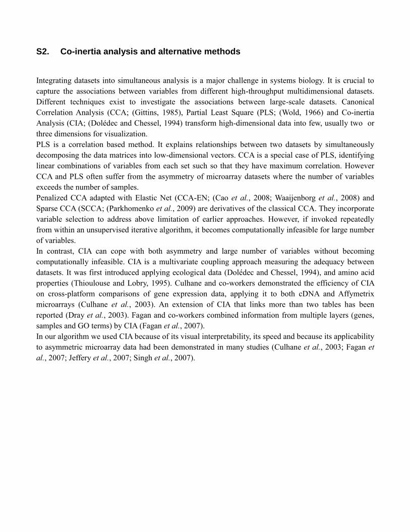
Distance matrix. Given two microarray datasets, let us assume r samples {r1, r2, …, rj} of dataset R and
b samples {b1, b2, …, bj} of dataset B. Projection of CIA sample distances on j-1 dimensions can be
plotted (Figure S1, top left). ω could be an (i j) distance matrix derived from CIA recording the
distance ω(ribj) between each pair of elements of R and B.
[5]
Weighted bipartite graph. The above distance matrix can be seen as a bipartite graph where each
vertex belongs to dataset R or B, and each edge corresponds to one element of the distance matrix (ω)
representing all inter-set distances of the CIA coordinates.
Here, the affiliation problem could be stated as given an ω, find j independent elements of permutation π
of {1, …, j} such that the sum of edge weights [6] is minimal for the selected edges.
Given a weighted bipartite graph where edge r->b has weight ω(rb),the optimal assignment minimizes
the overall weights. Figure S1 shows a graphical representation of the above.
[6]
r1
r2
r3
b1
b2
b3
Distances become
edge weights
ω1,1
ω3,3
R B
r1
r2
r3
b1
b2
b3
b1b2 b3
r1 ω1,1 ω1,2 ω1,3
r2 ω2,1 ω2,2 ω2,3
r3 ω3,1 ω3,2 ω3,3
ω - Weight Matrix
Hungarian
r1
r2
r3
b1
b2
b3
r1
r2
r3
b1
b2
b3
ω2,2
R B
=min
CIA distances in
j-1 dimensions
Figure S1. Affiliation of the connecting variables using Hungarian algorithm. Samples from R and B datasets are
represented as red and blue squares, respectively. Only samples are projected into 3-dimensional space for the simplicity
(top left). In the bipartite graph (top right) edges correspond to all pair-wise projected distances (weights) from every
element of R to all elements of B. Each edge corresponds to one element in the weight matrix ω recording these
distances. The Hungarian algorithm computes a matching of minimal distances (lower bipartite graph and lower 3d
plot).
S4. Cell-cycle data – cerevisiae versus pombe
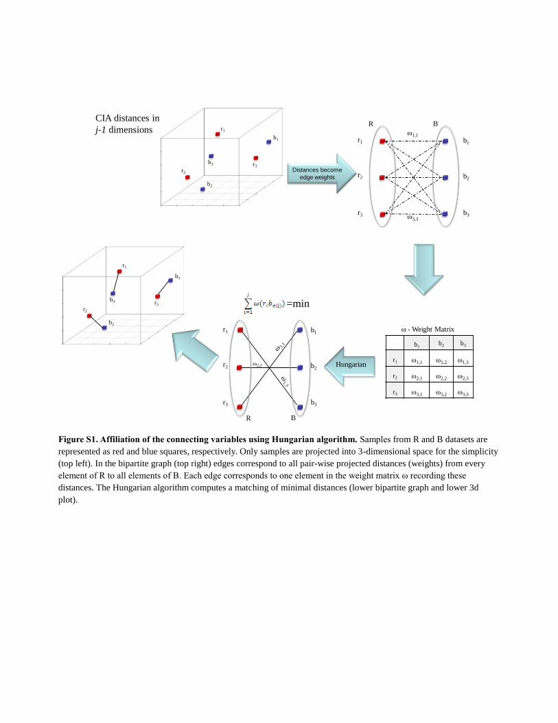
Figure S2. a) ‘Sce’ and ‘Sp’ projected by CIA. The affiliated samples of both datasets are connected by lines, the lengths of
which indicate the divergence between the two datasets. Each end of a line marks the position of a sample (time point) in
the projection. Each blue or red dot represents a gene of ‘Sce’ or ‘Sp’, respectively, its position determined by its relative
expression across all samples. The genes that are projected in the same direction from the centroid are those which are
highly expressed in that sample. b) ‘Spo’ dataset projected by CA. c)‘Sce’ dataset projected by CA.
Eigenvalues are shown in the bottom corner for each dataset, normalized to 100%. The first two (x and y) axes of ‘Sce’
explain 49% and 33% of the total inertia within this dataset. The first two axes of ‘Spo’ represent 64% and 30% of the total
variance within ‘Spo’. Thus more than 80% of the variance of the CIA was accounted for by the first two co-inertia axes and
thus presents a good summary of the co-structure between the two datasets.
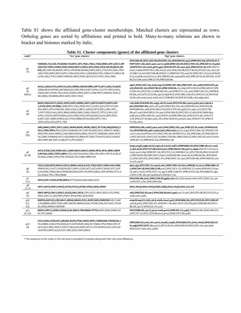
Table S1 shows the affiliated gene-cluster memberships. Matched clusters are represented as rows.
Ortholog genes are sorted by affiliations and printed in bold. Many-to-many relations are shown in
bracket and histones marked by italic.
Table S1. Cluster components (genes) of the affiliated gene clusters node† „Sce‟ gene clusters „Spo‟ gene clusters
g1 (7)
YOR292C,YJL123C,YFL034W,YCL047C,VIP1,TRA1,THG1,TCB3,SRM1,SPE1,SEC11,RPL30,PUS7,PRO1,PGM2,PDS5,OSH3,MOT1,HOG1,GPI1,ERJ5,CSE4,CDC20,(BCH1,BUD7),ISR1,HSP150,MCM5,YRF11,YPR203W,MCM3,CWP2,SED1,CTI6,SYP1,SOK1,YPL014W,TOS2,SMF3,GPI13,SPF1,CCR4,ACS2,HOL1,COS8,BIO2,FIN1,CIN8,SCY1,ERG3,YNL176C,AXL2,TOF2,CSM2,YGR035C,WSC2,PSA1,SEC53,FLC3,YEH1,SVS1,YNK1
SPAC3G6.05,SPCC1322.09,SPAC6F6.13c,SPAC694.03,asp1,SPBP16F5.03c,SPCC63.07,SPAPYUK71.03c,dcd1,spe1,sec11,rpl30,SPBC1A4.09,SPAC17H9.13c,SPBC32F12.10,pds5,SPAP27G11.01,mot1,phh1,gpi1,SPAC2E1P5.03,cnp1,slp1,SPBC31F10.16,SPBC19G7.04,atl1,mde6,SPAP27G11.08c,tim22,ask1,SPAC144.08,SPCC736.02,SPCC63.10c,mac1,SPCC1682.13,cki3,SPCC338.08,SPAC9.11,SPBP22H7.03,nup132,SPBC19C2.10,tas3,SPAC630.12,mrpl28,meu29,mrc1,cfh3,SPBC83.18c,vps8,phf2,set3,SPBC31F10.02,SPCC63.13,SPBC21C3.04c,bet5,SPBC27.04,SPBC428.06c
g2 (9,
M/G1)
ALG11,GAS5,HTZ1,KAP114,LEO1,MRM1,RAD54,RBG1,RPT5,SEY1,SSK2,YLL023C,GRX6,IRC19,SPP381,SNT309,GLO3,PIR3,YRF13,HXT7,GPA1,YIL177C,YRF12,PIG1,COQ4,SWF1,PCM1,TEL2,OCH1,ECM25,ERP3,GWT1,CHS6,PMT4,YIR043C,YOX1,ADK2,REB1,YKL069W,ERP2,WHI5,YHP1,TAO3
alg11,SPAC11E3.13c,mal1,kap114,SPBC13E7.08c,SPBC1347.13c,rad54,SPAC9.07c,pam2,SPAC222.14c,SPAPJ730.01,SPBC1539.04,chs2,klp5,SPCC320.03,SPBC16E9.07,SPBC15D4.01c,SPCC550.11,SPBC582.04c,csk1SPBC2F12.12c,urb2,SPBC1105.07c,SPAPB18E9.06c,nnf1,SPCC1223.04c,spc25,klp8,fkh2,SPAC19B12.08,cfh1,SPAC521.02,SPCP31B10.09,cdt1,imp2,arp2,mid2,mis17,SPBC8E4.04,SPAC3F10.08c,rid1,adg2,pht1
g3 (8)
BEM1,DID4,DUT1,(EXG1,SPR1),HOF1,MRN1,MSY1,(MYO3,MOY5),RSP5,SSO1,STU2,VPH1,YPL206C,FAR8,SPH1,TGL2,HEK2,POL12,GCR1,ALG14,PET112,RAD53,ANP1,HST4,YHR126C,ADE12,GLK1,UBP11,AAD10,SPT3,RED1,JSN1,YRF1_7,GYP7,PFK1,FAA1,EXO1,RMA1,MDS3,SWE1,SUB1,YDL027C,YPT11,CSH1,CDC9,PXL1,CDC45,EMP70,MSH2,ELG1,FRE6,VID22,SPO16,EXG2,SLD2,UBP3,POL30,ASF1,OST2,BNI5,PDR16,GIC1,PHS1,RRN9,GPI16,SFB3,OPY2 ,FHL1 ,SHO1,CKS1,SVL3,ATF1, FIR1
ral3,did4,SPAC644.05c,exg1,cdc15,msa2,SPCC576.06c,myo1,pub1,psy1,alp14,vph1,SPAC4D7.02c,etd1,ntf1,pof3,SPBC24C6.10c,cdt2,SPBC405.02c,SPAC4H3.06,SPAPJ698.04c,set8,SPAC19G12.05,SPAC17H9.18c,ppk3,fin1,alp1,orc5,SPCC794.08,rpl7,nse5,SPAC30D11.01c,psc3,SPAC3G9.05,SPCC320.12,cfh4,SPAC24H6.08,ppc89,par2,SPBC1306.01c,set2,SPAC9.10,SPBC29A3.03c,SPAC2E1P5.02c,SPAC1F12.05,SPAC227.05,fep1,lad1,cfh2,SPAC1639.01c,pmp31,ulp1,SPAC977.01,SPBC14F5.10c,cdm1
g4 (10)
AIR2,BMH1,DDP1,ENT1,GAS1,HEM4,MDR1,MOB1,MSE1,RTT106,SNQ2SSK22,STE11,TFB4,TRP4,SPO12,KIP3,YLR462W,FAT1,HXT10,EMI2,GEF1,YER071C,MSB1,DDI2,PRI2,SHE3,YMR31,CLB5,SNO3,PHO3,MSA1,YEL077C,YMR258C,HAA1,PEX7,YJL218W,YLR464W,AVT2,YGL036W,IST2,BNI4,RTT109,CTF4,HXT2,RCO1,GCN5,PDR5,YMR118C,SNT1,CLB6,EPT1,LPP1,RAD27
SPBP35G2.08c,rad25,aps1,ent1,SPAC19B12.02c,ups,SPBC215.01,mob1,SPAPB1A10.11c,SPAC6G9.03c,pdr1,wak1,byr2,tfb4,trp4,apc15,mog1,SPAC13G6.10c,SPAC821.03c,hrr1,meu34,SPCC613.07,SPAC1705.03c,SPAPB17E12.10c,SPBC1861.07,SPAC5D6.02c,SPCC16C4.02c,SPAC11E3.10,SPBC17G9.06c,SPBC15D4.02,SPAC1565.02c,efc25,hmt1,SPBC3H7.13,SPBP4H10.16c,SPBPB2B2.19c
g5 (6, M)
ACF2,ATG8,CLB2,ERG6,HSL1,LSM2,MCD1,MUC1,NOB1,RER1,RFA1,RNR1,RRP45,RVS161,SEN1,TOP2,UBP6,YCK1,CAF120,HCM1,STB1,LSP1,ERS1,YRF15,ALD6,STE2,RGA1,CMK1,YPR157W,YCR102C,YDL118W,YBR071W
(eng1,eng2),atg8,cdc13,erg6,cdr1,lsm2,rad21,SPBPJ4664.02,SPAC1486.09,rer1,rad11,ssb1,dc22,SPCC757.08,hob3,(sen1,SPBC29A10.10c),ptr11,ubp6,SPAC3C7.07c,hcn1,mcp1,pus2,chp2,SPBC947.14c,SPCC576.12c,SPAP8A3.11c,SPCC794.03,SPAC15A10.09c,SPBC29A10.08,SPBC14C8.13,bet1,SPAC630.04c,rho4,cdc25,SPBC36.06c,SPAC26H5.11,SPAC14C4.05c,SPAC24B11.07c,SPBC16H5.12c,vip1,SPCC594.04c,SPAP14E8.02,cam2,csx2,ucp10
g6 (5)
CDC5,CLB3,ENT3,MYO1,POL31,RKM1,SAC6,SLY41,TFB3,VID27,VRG4,YDL124W,FMP45,KEL2,VHT1,YFL067W,RLF2,DPH1,CUE4,GET1,KCC4,REV7,SKG6,SUT1,GYP6,YHL026C,PMA2,IRC4,YPR202W,RAD2,NUP170,APA2,NRG2,UIP5,WTM2,STV1,ALE1,GGA2,TPK1,TRK2,MSB4
plo1,cig1,SPCC794.11c,myo3,cdc1,SPBC1709.13c,fim1,SPBC83.11,mcr1,SPBC1685.14c,SPAC144.18,SPAC19G12.09,ace2,SPAC14C4.12c,SPBC4F6.12,mrpl4,SPAC4G9.19,rpc31,aph1,mrp51,SPAC27D7.11c,agn1,SPBC1198.07c,SPBC31F10.10c,SPAC688.07c,dga1,SPCC1795.10c,spTrap240,af1,SPAC637.13c
g7 (11)
ADY2,CDC7,COG3,GPI8,SMC4,GTT3,GAS3,GAS4,GAS2,GLE1
SPAC5D6.09c,hsk1,SPBC1539.05,gpi8,cut3,sfc2,clr8,myo52,mbx1,SPCC1020.12c,rum1,SPCC4F11.03c,SPAC20H4.05c
g8 (1, S)
HHT1,HHT2,(HHF1,HHF2),(HTA2,HTA1),(HTB2,HTB1),HDA1,RPD3
(hht1,hht2),(hht1,hht3),(hhf1,hhf2),(hta1,hta2),htb1,clr3,clr6
g9 (2)
DBF2,INP53,OAC1,(ODC1,OCD2),RAI1,SEC4,COP1,ECO1,ARV1,RSF2,LYS1,DPB2,HSD1,CDC11,CLN2,PMT5,PMT1,RFA3,PIN2,SAS3,FKH2
sid2,SPBC2G2.02,oac1,SPAC328.09,din1,ypt2,sec72,sad1,SPCC970.08,SPCC553.07c,prp28,cam1,spd1
g10 (12, G1)
EMP24,KAP122,LCB2,MLC1,MSH6,MSW1,POL1,RUP2,SKI3,YMR259C,HSL7,HAP2,YDL089W,QDR3,TOS4,UBX7,MCM2,MMS4,GGA1,PHO8,COS4,SVF1,HIF1,YFL042C,HOS3,AIM34,YLR455W
emp24,kap111,lcb2,cdc4,msh6,msw1,pol1,SPAPJ696.03c,SPCC1919.05,SPCC1494.07,cdc18,pnk1,SPBC25B2.07c,SPAC8F11.06,dfp1,SPCC1235.09,pkd2,SPBC660.06,SPCC188.10c,rpc17,SPAC2C4.17c,cut2
g11 (3, G2)
MSS51,RPC11,(SIM1,SUN4),SLA2,SMC3,YML096W,YPT52,KAR5,DSN1,DAM1,FKH1,FIP1,MSA2
SPAC25B8.04c,rpc11,psu1,end4,psm3,SPBC4F6.11c,ypt5,SPBC4C3.04c,SPAC10F6.07c,SPCC757.12,SPCC1259.08,ams2,pmc2,SPAC27D7.09c,pdf1
g12 (4)
CCC2,CDH1,CHS5,IPL1,MUS81,NUP2,PTM1,RHO1,RPP1,YMR244W,YOR291W,GFA1,MSB2,CLN3,CYS3,ESC8,ALY2,HXT4,ROD1,MAL33,TCM62,TPS2,PAN2,HST2,PUF4,CAC2,ORC1,PEX11,HXT5,TUB2,SLN1,RDS2,SPT21,CTF18,INP2,EUG1,SFG1,MCD4,PRY2,NPP2,GLG2,FCP1,PBI2,SGS1,CRH1,RHO3
SPBC29A3.01,srw1,cfr1,aim1,mus81,nup61,SPAC26H5.07c,(rho1,rho5),SPAC3A12.04c,adg3,SPCC1672.11c,spo12,SPCC126.01c,SPAC3H8.03,SPAC10F6.14c,ssp1,klp6 SPAC11H11.02c,zds1,cwf25
† The sequence of the nodes in the cell cycle is provided in brackets along with their cell cycle affiliations.
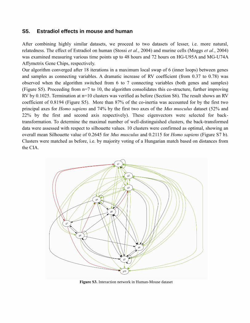
S5. Estradiol effects in mouse and human
After combining highly similar datasets, we proceed to two datasets of lesser, i.e. more natural,
relatedness. The effect of Estradiol on human (Stossi et al., 2004) and murine cells (Moggs et al., 2004)
was examined measuring various time points up to 48 hours and 72 hours on HG-U95A and MG-U74A
Affymetrix Gene Chips, respectively.
Our algorithm converged after 18 iterations in a maximum local swap of 6 (inner loops) between genes
and samples as connecting variables. A dramatic increase of RV coefficient (from 0.37 to 0.78) was
observed when the algorithm switched from 6 to 7 connecting variables (both genes and samples)
(Figure S5). Proceeding from n=7 to 10, the algorithm consolidates this co-structure, further improving
RV by 0.1025. Termination at n=10 clusters was verified as before (Section S6). The result shows an RV
coefficient of 0.8194 (Figure S5). More than 87% of the co-inertia was accounted for by the first two
principal axes for Homo sapiens and 74% by the first two axes of the Mus musculus dataset (52% and
22% by the first and second axis respectively). These eigenvectors were selected for back-
transformation. To determine the maximal number of well-distinguished clusters, the back-transformed
data were assessed with respect to silhouette values. 10 clusters were confirmed as optimal, showing an
overall mean Silhouette value of 0.2645 for Mus musculus and 0.2115 for Homo sapiens (Figure S7 b).
Clusters were matched as before, i.e. by majority voting of a Hungarian match based on distances from
the CIA.
Figure S3. Interaction network in Human-Mouse dataset

Based on the two back-transformed data tables, we represented each cluster by the gene-wise sum of all
comprised genes across both tables. Subjecting this combined table to reverse engineering, these cluster
representatives became the nodes of a common gene network (Figure S3). TP edges are shown in green,
FN are shown in black, FP or (previously unknown interactions) are shown in red. Out of 100 observed
interactions 40 were true positives, 5 false positives, 26 false negatives and 29 true negatives, yielding a
sensitivity of 60% and a specificity of 85%. Remarkably, the accuracy of 69% is comparable to the yeast
common regulatory network.
Compared to the yeast common regulatory network we observe a shift from specificity (decreased) to
sensitivity (increased). It remains unclear, however, if all edges counted as false positives for not being
part of our "true network" are actually incorrect. Some of them could represent true interactions not yet
represented in KEGG or any of the other databases we used as reference. Thus, above shift could simply
mean fewer edges which are reported (as opposed to observed) in the estradiol context and thus should
not be over interpreted in terms of algorithm performance.
We further characterized the statistical significance of comprised network motifs as a function of the
network size, by considering sub networks of the full network. The frequency of motifs in the sub
networks of the common network of 10 nodes is significantly higher comparing to larger networks
(Figure S9). The decrease of the motif concentration with network sizes larger than 10 agrees both with
RV-based selection of n and optimal Silhouette values. In general, the larger the network, the more
frequent motifs should become. Here, their decrease indicates a lack of robustness for delineated
networks of more than 10 nodes, corroborating the number automatically chosen by our algorithm.
S6. Evaluation of optimal granularity
S6.1 Gradual improvement of RV coefficients
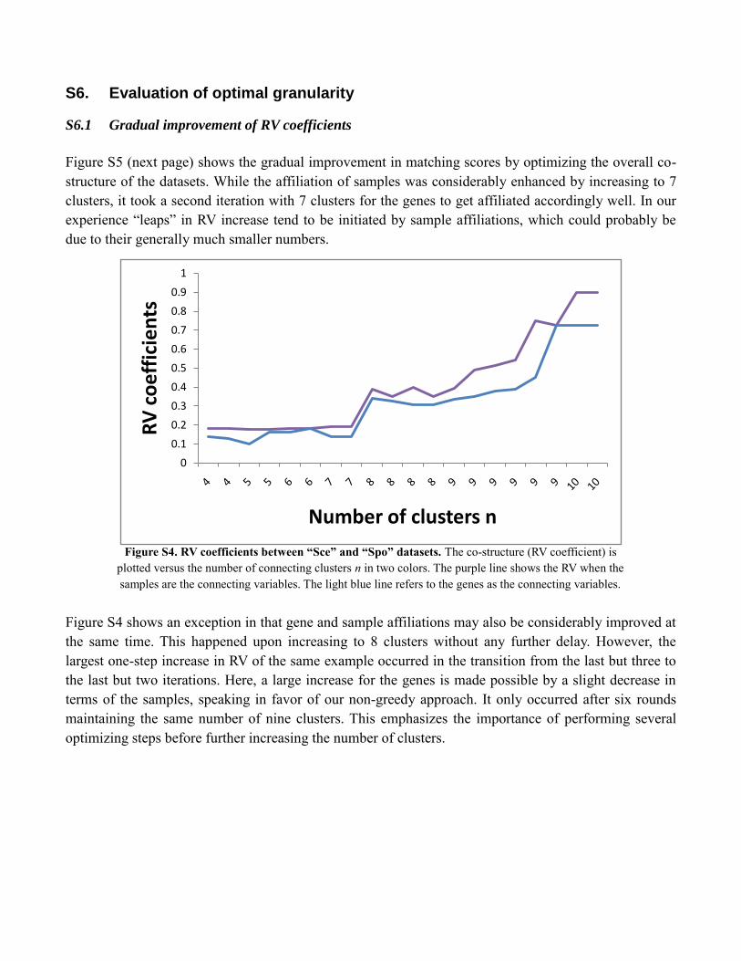
Figure S5 (next page) shows the gradual improvement in matching scores by optimizing the overall co-
structure of the datasets. While the affiliation of samples was considerably enhanced by increasing to 7
clusters, it took a second iteration with 7 clusters for the genes to get affiliated accordingly well. In our
experience “leaps” in RV increase tend to be initiated by sample affiliations, which could probably be
due to their generally much smaller numbers.
Figure S4 shows an exception in that gene and sample affiliations may also be considerably improved at
the same time. This happened upon increasing to 8 clusters without any further delay. However, the
largest one-step increase in RV of the same example occurred in the transition from the last but three to
the last but two iterations. Here, a large increase for the genes is made possible by a slight decrease in
terms of the samples, speaking in favor of our non-greedy approach. It only occurred after six rounds
maintaining the same number of nine clusters. This emphasizes the importance of performing several
optimizing steps before further increasing the number of clusters.
Figure S4. RV coefficients between “Sce” and “Spo” datasets. The co-structure (RV coefficient) is
plotted versus the number of connecting clusters n in two colors. The purple line shows the RV when the
samples are the connecting variables. The light blue line refers to the genes as the connecting variables.
0
0.1
0.2
0.3
0.4
0.5
0.6
0.7
0.8
0.9
1
RV
co
eff
icie
nts
Number of clusters n
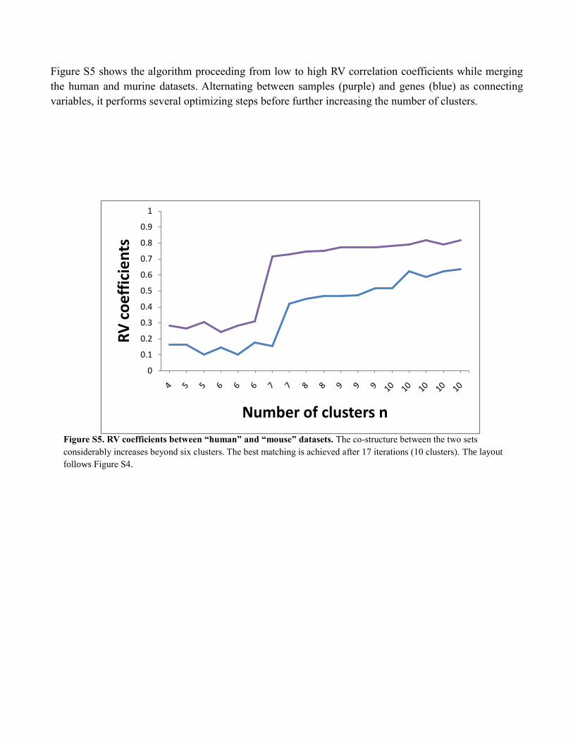
Figure S5 shows the algorithm proceeding from low to high RV correlation coefficients while merging
the human and murine datasets. Alternating between samples (purple) and genes (blue) as connecting
variables, it performs several optimizing steps before further increasing the number of clusters.
Figure S5. RV coefficients between “human” and “mouse” datasets. The co-structure between the two sets
considerably increases beyond six clusters. The best matching is achieved after 17 iterations (10 clusters). The layout
follows Figure S4.
0
0.1
0.2
0.3
0.4
0.5
0.6
0.7
0.8
0.9
1
RV
co
eff
icie
nts
Number of clusters n
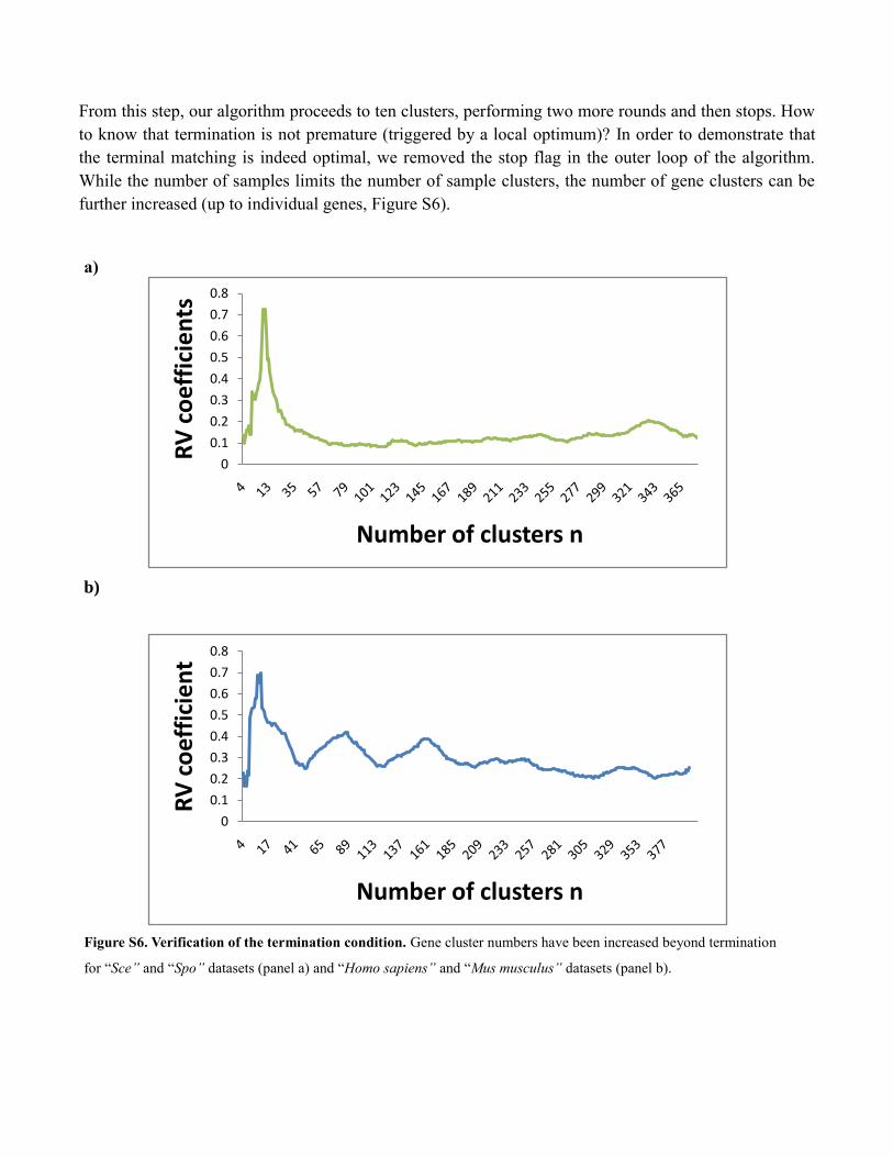
From this step, our algorithm proceeds to ten clusters, performing two more rounds and then stops. How
to know that termination is not premature (triggered by a local optimum)? In order to demonstrate that
the terminal matching is indeed optimal, we removed the stop flag in the outer loop of the algorithm.
While the number of samples limits the number of sample clusters, the number of gene clusters can be
further increased (up to individual genes, Figure S6).
a)
b)
Figure S6. Verification of the termination condition. Gene cluster numbers have been increased beyond termination
for “Sce” and “Spo” datasets (panel a) and “Homo sapiens” and “Mus musculus” datasets (panel b).
0
0.1
0.2
0.3
0.4
0.5
0.6
0.7
0.8
RV
co
eff
icie
nts
Number of clusters n
0
0.1
0.2
0.3
0.4
0.5
0.6
0.7
0.8
RV
co
eff
icie
nt
Number of clusters n

The optimal number of gene clusters for the combination depends on how many clusters can be
discriminated in each dataset (Figure S7). Figure S7a, shows silhouette values for the yeast datasets. As
the number of clusters increases silhouette values decrease from 0.3935 (for 2 clusters) down to -0.2154
(140 clusters) in “Sce” and from 0.4987 to -0.0731 in “Spo”. The overall optima of 0.3504 and 0.3921
were obtained for maximally 12 well separated gene clusters.
Figure S7. Silhouette values. Panel a) plots the quality of the clustering depending on the number of clusters for “Sce”
(red line) and “Spo” (blue) . “Homo sapiens” (red) and “Mus musculus” (blue) are shown in panel b.

S6.2 Receiver Operating Characteristics (ROC)
We applied ROC curves in order to study different granularities for both the Saccharomyces/pombe and
the human/mouse merges (Figure S8). The method is described in detail by Swets and Pickett (1982).
Here, each point depicts a common network compared to known interactions (expected network) derived
from various data sources (Table S3). The pathway databases were queried using the Ingenuity Pathway
Analysis in order not to miss any existing interaction as described in the method section.
The cluster number n is plotted next to each data point. Both curves show similar increases in false
positive rates when progressing to larger n.
Figure S8. ROC curves.
The sensitivity is plotted against the specificity for “Sce” /“Spo” (blue) and mouse/human (green)
common networks. Numbers annotate the number of clusters n (granularity) used for the common
network. The diagonal dashed line is the expected ROC curve of a random predictor.
12
13
14
15 1618 17
19
10
1112
1314
15
1617
0
0.1
0.2
0.3
0.4
0.5
0.6
0.7
0.8
0.9
1
0 0.2 0.4 0.6 0.8 1
Tru
e p
osi
tive
rat
es
False positive rates

S6.3 Significance Analysis of Network Motifs
Significance of network motifs for a specific network is studied by Z-Score and p-Value (as described in
the methods section). Significance profiles on the basis of the Z-scores can be used to compare different
networks. Furthermore, the frequency of motifs can directly be used for network evaluation.
In our analysis motifs of sizes three and four are assessed to compare different directed networks. While
the number of non-isomorphic motifs grows exponentially with the size of the motifs, in practice, only a
fraction of all possible motifs is implemented by real biological networks. Up to the present time, known
network motifs are small and usually comprise three to five vertices only.
For the calculation of the statistical significance of network motifs we used a commonly used method
that compares the number of the observed network motifs to the concentration of the motifs in an
ensemble randomized network. Therefore, calculation of the motif statistics requires the consideration of
several hundreds to thousands of randomized networks.
The size of the observed network determines the number of motifs. In general it is expected for the
number of significant motifs to increase with the size of the network. Interestingly, in our analysis we
obtained highest number of significant motifs in the smaller networks, corroborating the authenticity of
our common network.
a)
b)
Figure S9. Significance of motifs in the mouse / human consensus network. The number of motifs (size-3 and size-4
in panels „a‟ and „b‟, respectively) is plotted versus the network size. The number of discovered motifs decreases with
the number of clusters n used for combining the datasets (network size).
0
2
4
6
8
Nu
mb
er o
f m
oti
fs
Network size
0
20
40
60
10 100 200 300 400
Nu
mb
er o
f m
oti
fs
Network size
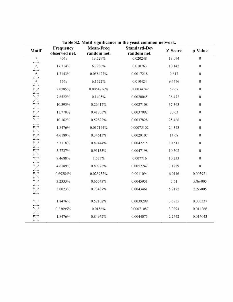
Table S2. Motif significance in the yeast common network.
Motif Frequency
observed net.
Mean-Freq
random net.
Standard-Dev
random net. Z-Score p-Value
40% 13.529% 0.020248 13.074 0
17.714% 6.7986% 0.010763 10.142 0
1.7143% 0.058427% 0.0017218 9.617 0
16% 6.1522% 0.010424 9.4476 0
2.0785% 0.0054736% 0.00034742 59.67 0
7.8522% 0.1405% 0.0020045 38.472 0
10.393% 0.26417% 0.0027108 37.363 0
11.778% 0.41705% 0.0037092 30.63 0
10.162% 0.52822% 0.0037828 25.466 0
1.8476% 0.017144% 0.00075102 24.373 0
4.6189% 0.34613% 0.0029107 14.68 0
5.3118% 0.87444% 0.0042215 10.511 0
5.7737% 0.91135% 0.0047198 10.302 0
9.4688% 1.573% 0.007716 10.233 0
4.6189% 0.89778% 0.0052242 7.1229 0
0.69284% 0.025932% 0.0011094 6.0116 0.003921
3.2333% 0.65543% 0.0045951 5.61 5.8e-005
3.0023% 0.73487% 0.0043461 5.2172 2.2e-005
1.8476% 0.52102% 0.0039299 3.3755 0.003337
0.23095% 0.0156% 0.00071087 3.0294 0.014266
1.8476% 0.84962% 0.0044075 2.2642 0.016043
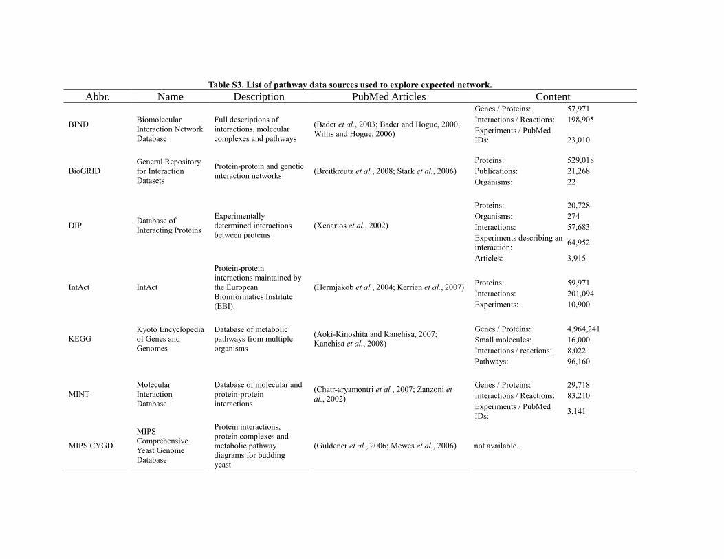
Table S3. List of pathway data sources used to explore expected network.
Abbr. Name Description PubMed Articles Content
BIND
Biomolecular
Interaction Network
Database
Full descriptions of
interactions, molecular
complexes and pathways
(Bader et al., 2003; Bader and Hogue, 2000;
Willis and Hogue, 2006)
Genes / Proteins: 57,971
Interactions / Reactions: 198,905
Experiments / PubMed
IDs:
23,010
BioGRID
General Repository
for Interaction
Datasets
Protein-protein and genetic
interaction networks (Breitkreutz et al., 2008; Stark et al., 2006)
Proteins: 529,018
Publications: 21,268
Organisms: 22
DIP Database of
Interacting Proteins
Experimentally
determined interactions
between proteins
(Xenarios et al., 2002)
Proteins: 20,728
Organisms: 274
Interactions: 57,683
Experiments describing an
interaction: 64,952
Articles: 3,915
IntAct IntAct
Protein-protein
interactions maintained by
the European
Bioinformatics Institute
(EBI).
(Hermjakob et al., 2004; Kerrien et al., 2007)
Proteins: 59,971
Interactions: 201,094
Experiments: 10,900
KEGG
Kyoto Encyclopedia
of Genes and
Genomes
Database of metabolic
pathways from multiple
organisms
(Aoki-Kinoshita and Kanehisa, 2007;
Kanehisa et al., 2008)
Genes / Proteins: 4,964,241
Small molecules: 16,000
Interactions / reactions: 8,022
Pathways: 96,160
MINT
Molecular
Interaction
Database
Database of molecular and
protein-protein
interactions
(Chatr-aryamontri et al., 2007; Zanzoni et
al., 2002)
Genes / Proteins: 29,718
Interactions / Reactions: 83,210
Experiments / PubMed
IDs: 3,141
MIPS CYGD
MIPS
Comprehensive
Yeast Genome
Database
Protein interactions,
protein complexes and
metabolic pathway
diagrams for budding
yeast.
(Guldener et al., 2006; Mewes et al., 2006) not available.
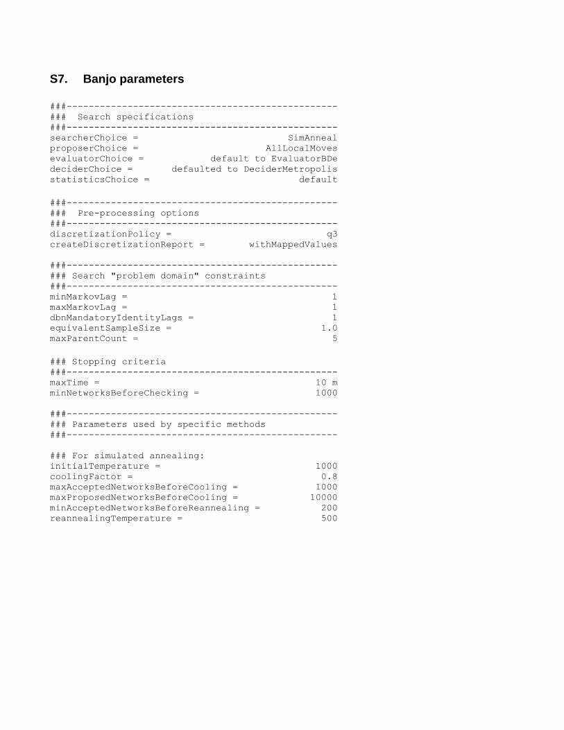
S7. Banjo parameters
###-------------------------------------------------
### Search specifications
###-------------------------------------------------
searcherChoice = SimAnneal
proposerChoice = AllLocalMoves
evaluatorChoice = default to EvaluatorBDe
deciderChoice = defaulted to DeciderMetropolis
statisticsChoice = default
###-------------------------------------------------
### Pre-processing options
###-------------------------------------------------
discretizationPolicy = q3
createDiscretizationReport = withMappedValues
###-------------------------------------------------
### Search "problem domain" constraints
###-------------------------------------------------
minMarkovLag = 1
maxMarkovLag = 1
dbnMandatoryIdentityLags = 1
equivalentSampleSize = 1.0
maxParentCount = 5
### Stopping criteria
###-------------------------------------------------
maxTime = 10 m
minNetworksBeforeChecking = 1000
###-------------------------------------------------
### Parameters used by specific methods
###-------------------------------------------------
### For simulated annealing:
initialTemperature = 1000
coolingFactor = 0.8
maxAcceptedNetworksBeforeCooling = 1000
maxProposedNetworksBeforeCooling = 10000
minAcceptedNetworksBeforeReannealing = 200
reannealingTemperature = 500

S8. Cell cycle datasets of the same species
For the previous data examples, evaluation of the common gene network suffers from incomplete
knowledge of interactions among all genes. In the same way, ortholog affiliations were not available for
each gene. In order to reliably know all gene affiliations in advance, we performed the matching
algorithm on two S. pombe cell cycle experiments described by (Oliva et al., 2005) and (Rustici et al.,
2004). The algorithm was performed using a procedure identical to that applied to the previous yeast cell
cycle datasets (section S4 as well as section 3.2 of the manuscript):
S8.1. Estimation of periodic genes in the cell cycle
S8.2. Running the matching algorithm
S8.3. Refinement
S8.4. CIA plot of sample and gene cluster affiliations
S8.1. Estimation of periodic genes in the cell cycle
Two different laboratories used DNA microarrays to study periodic gene expression program of the
fission yeast cell cycle. We used the normalized datasets named “elutriation 1” (Rustici et al., 2004) and
“elutriation A” (Oliva et al., 2005), each relating to individual experiments. We will refer to these data
sets as ‘ds1’ and ‘ds2’, respectively. We selected the first cell cycle period (10 time points) from both
datasets for perfect synchronization. The total number of genes found to oscillate with a FDR of 0.1 in
the first study was 1060, whereas in the second study 360 genes were identified. Of those, 337 were
found in both. These genes, as well as the samples, were permuted (anonymized) and used as an input to
our algorithm.
S8.2. Running the matching algorithm
The algorithm terminated after 12 iterations, with maximal two inner loops, resulting in an RV
coefficient of 0.9356. In theory, the optimal pairing could be determined by evaluating all possible
pairings as in the initialization step. However, n×n! evaluation steps are not feasible for larger n. This
would require 3.6×10⁷ instead of the 35 CIA executed until convergence. Termination at n=10 clusters
was verified as before (RV improvement and Silhouette values).
The result was visualized by CIA (Figure S10). The first two (x and y) axes of „ds1‟ explain 72% and
25% of the total inertia, respectively. The first two axes of „ds2‟ represent 71% and 22% of the total
variance within „ds2‟. Thus more than 90% of the variance of the CIA was accounted for by the first two
co-inertia axes and thus presents a good summary of the co-structure between the two datasets.
S8.3. Refinement
A maximum of 10 well separated gene clusters were obtained in the refinement step with overall
silhouette values of 0.42 and 0.44 for „ds1‟ and „ds2‟, respectively. Increasing the number of gene
clusters from 10 to 17, the overall silhouette values would almost remain the same (differing by less than
0.01 for each dataset). However, the best RV was obtained for n=10. This suggests an optimum
similarity when datasets are clustered into 10 gene clusters only.

S8.4. CIA plot of sample and gene cluster affiliations.
Figure S10. „ds1‟ and „ds2‟ projected by CIA.
Affiliated samples of both datasets are connected by lines. Each red or blue number represents samples (time points), and
each dot or „+‟ depicts a gene of ‘ds1’ or ‘ds2’, respectively. Affiliated gene clusters are highlighted in same colors.
Histones are encircled in grey.
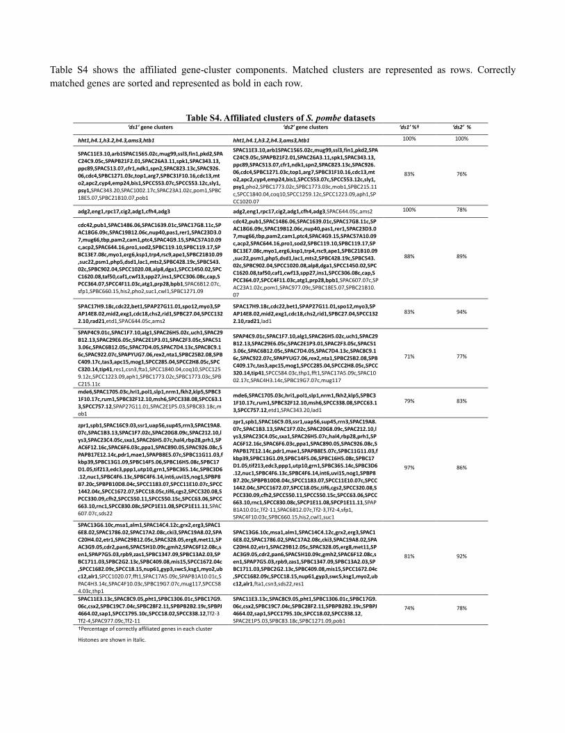
Table S4 shows the affiliated gene-cluster components. Matched clusters are represented as rows. Correctly
matched genes are sorted and represented as bold in each row.
Table S4. Affiliated clusters of S. pombe datasets ‘ds1’ gene clusters ‘ds2’ gene clusters ‘ds1’ %† ‘ds2’ %
hht1,h4.1,h3.2,h4.3,ams3,htb1 hht1,h4.1,h3.2,h4.3,ams3,htb1 100% 100%
SPAC11E3.10,arb1SPAC1565.02c,mug99,ssl3,fin1,pkd2,SPAC24C9.05c,SPAPB21F2.01,SPAC26A3.11,spk1,SPAC343.13,ppc89,SPAC513.07,cfr1,ndk1,spn2,SPAC823.13c,SPAC926.06,cdc4,SPBC1271.03c,top1,arg7,SPBC31F10.16,cdc13,mto2,apc2,cyp4,emp24,bis1,SPCC553.07c,SPCC553.12c,sly1,psy1,SPAC343.20,SPAC1002.17c,SPAC23A1.02c,pom1,SPBC18E5.07,SPBC21B10.07,pob1
SPAC11E3.10,arb1SPAC1565.02c,mug99,ssl3,fin1,pkd2,SPAC24C9.05c,SPAPB21F2.01,SPAC26A3.11,spk1,SPAC343.13,ppc89,SPAC513.07,cfr1,ndk1,spn2,SPAC823.13c,SPAC926.06,cdc4,SPBC1271.03c,top1,arg7,SPBC31F10.16,cdc13,mto2,apc2,cyp4,emp24,bis1,SPCC553.07c,SPCC553.12c,sly1,psy1,pho2,SPBC1773.02c,SPBC1773.03c,mob1,SPBC215.11c,SPCC1840.04,coq10,SPCC1259.12c,SPCC1223.09,aph1,SPCC1020.07
83% 76%
adg2,eng1,rpc17,cig2,adg1,cfh4,adg3 adg2,eng1,rpc17,cig2,adg1,cfh4,adg3,SPAC644.05c,ams2 100% 78%
cdc42,pub1,SPAC1486.06,SPAC1639.01c,SPAC17G8.11c,SPAC18G6.09c,SPAC19B12.06c,nup40,pas1,rer1,SPAC23D3.07,mug66,tbp,pam2,cam1,ptc4,SPAC4G9.15,SPAC57A10.09c,acp2,SPAC644.16,pro1,sod2,SPBC119.10,SPBC119.17,SPBC13E7.08c,myo1,erg6,ksp1,trp4,rsc9,ape1,SPBC21B10.09,suc22,psm1,php5,dsd1,lac1,mts2,SPBC428.19c,SPBC543.02c,SPBC902.04,SPCC1020.08,alp8,dga1,SPCC1450.02,SPCC1620.08,taf50,caf1,cwf13,spp27,ins1,SPCC306.08c,cap,SPCC364.07,SPCC4F11.03c,atg1,prp28,bpb1,SPAC6B12.07c,sfp1,SPBC660.15,his2,pho2,suc1,cwl1,SPBC1271.09
cdc42,pub1,SPAC1486.06,SPAC1639.01c,SPAC17G8.11c,SPAC18G6.09c,SPAC19B12.06c,nup40,pas1,rer1,SPAC23D3.07,mug66,tbp,pam2,cam1,ptc4,SPAC4G9.15,SPAC57A10.09c,acp2,SPAC644.16,pro1,sod2,SPBC119.10,SPBC119.17,SPBC13E7.08c,myo1,erg6,ksp1,trp4,rsc9,ape1,SPBC21B10.09,suc22,psm1,php5,dsd1,lac1,mts2,SPBC428.19c,SPBC543.02c,SPBC902.04,SPCC1020.08,alp8,dga1,SPCC1450.02,SPCC1620.08,taf50,caf1,cwf13,spp27,ins1,SPCC306.08c,cap,SPCC364.07,SPCC4F11.03c,atg1,prp28,bpb1,SPAC607.07c,SPAC23A1.02c,pom1,SPAC977.09c,SPBC18E5.07,SPBC21B10.07
88% 89%
SPAC17H9.18c,cdc22,bet1,SPAP27G11.01,spo12,myo3,SPAP14E8.02,mid2,exg1,cdc18,chs2,rid1,SPBC27.04,SPCC1322.10,rad21,etd1,SPAC644.05c,ams2
SPAC17H9.18c,cdc22,bet1,SPAP27G11.01,spo12,myo3,SPAP14E8.02,mid2,exg1,cdc18,chs2,rid1,SPBC27.04,SPCC1322.10,rad21,lad1
83% 94%
SPAP4C9.01c,SPAC1F7.10,alg1,SPAC26H5.02c,uch1,SPAC29B12.13,SPAC29E6.05c,SPAC2E1P3.01,SPAC2F3.05c,SPAC513.06c,SPAC6B12.05c,SPAC7D4.05,SPAC7D4.13c,SPAC8C9.16c,SPAC922.07c,SPAPYUG7.06,rex2,nta1,SPBC25B2.08,SPBC409.17c,tas3,apc15,mog1,SPCC285.04,SPCC2H8.05c,SPCC320.14,tip41,res1,csn3,fta1,SPCC1840.04,coq10,SPCC1259.12c,SPCC1223.09,aph1,SPBC1773.02c,SPBC1773.03c,SPBC215.11c
SPAP4C9.01c,SPAC1F7.10,alg1,SPAC26H5.02c,uch1,SPAC29B12.13,SPAC29E6.05c,SPAC2E1P3.01,SPAC2F3.05c,SPAC513.06c,SPAC6B12.05c,SPAC7D4.05,SPAC7D4.13c,SPAC8C9.16c,SPAC922.07c,SPAPYUG7.06,rex2,nta1,SPBC25B2.08,SPBC409.17c,tas3,apc15,mog1,SPCC285.04,SPCC2H8.05c,SPCC320.14,tip41,SPCC584.03c,thp1,fft1,SPAC17A5.09c,SPAC1002.17c,SPAC4H3.14c,SPBC19G7.07c,mug117
71% 77%
mde6,SPAC1705.03c,hri1,pol1,slp1,nrm1,fkh2,klp5,SPBC31F10.17c,rum1,SPBC32F12.10,msh6,SPCC338.08,SPCC63.13,SPCC757.12,SPAP27G11.01,SPAC2E1P5.03,SPBC83.18c,mob1
mde6,SPAC1705.03c,hri1,pol1,slp1,nrm1,fkh2,klp5,SPBC31F10.17c,rum1,SPBC32F12.10,msh6,SPCC338.08,SPCC63.13,SPCC757.12,etd1,SPAC343.20,lad1
79% 83%
zpr1,spb1,SPAC16C9.03,ssr1,uap56,sup45,rrn3,SPAC19A8.07c,SPAC1B3.13,SPAC1F7.02c,SPAC20G8.09c,SPAC212.10,lys3,SPAC23C4.05c,sxa1,SPAC26H5.07c,hal4,rbp28,prh1,SPAC6F12.16c,SPAC6F6.03c,ppa1,SPAC890.05,SPAC926.08c,SPAPB17E12.14c,pdr1,mae1,SPAPB8E5.07c,SPBC11G11.03,fkbp39,SPBC13G1.09,SPBC14F5.06,SPBC16H5.08c,SPBC17D1.05,tif213,edc3,ppp1,utp10,grn1,SPBC365.14c,SPBC3D6.12,nuc1,SPBC4F6.13c,SPBC4F6.14,int6,uvi15,nog1,SPBP8B7.20c,SPBPB10D8.04c,SPCC1183.07,SPCC11E10.07c,SPCC1442.04c,SPCC1672.07,SPCC18.05c,tif6,cgs2,SPCC320.08,SPCC330.09,cfh2,SPCC550.11,SPCC550.15c,SPCC63.06,SPCC663.10,rnc1,SPCC830.08c,SPCP1E11.08,SPCP1E11.11,SPAC607.07c,sds22
zpr1,spb1,SPAC16C9.03,ssr1,uap56,sup45,rrn3,SPAC19A8.07c,SPAC1B3.13,SPAC1F7.02c,SPAC20G8.09c,SPAC212.10,lys3,SPAC23C4.05c,sxa1,SPAC26H5.07c,hal4,rbp28,prh1,SPAC6F12.16c,SPAC6F6.03c,ppa1,SPAC890.05,SPAC926.08c,SPAPB17E12.14c,pdr1,mae1,SPAPB8E5.07c,SPBC11G11.03,fkbp39,SPBC13G1.09,SPBC14F5.06,SPBC16H5.08c,SPBC17D1.05,tif213,edc3,ppp1,utp10,grn1,SPBC365.14c,SPBC3D6.12,nuc1,SPBC4F6.13c,SPBC4F6.14,int6,uvi15,nog1,SPBP8B7.20c,SPBPB10D8.04c,SPCC1183.07,SPCC11E10.07c,SPCC1442.04c,SPCC1672.07,SPCC18.05c,tif6,cgs2,SPCC320.08,SPCC330.09,cfh2,SPCC550.11,SPCC550.15c,SPCC63.06,SPCC663.10,rnc1,SPCC830.08c,SPCP1E11.08,SPCP1E11.11,SPAPB1A10.01c,Tf2-11,SPAC6B12.07c,Tf2-3,Tf2-4,sfp1, SPAC4F10.03c,SPBC660.15,his2,cwl1,suc1
97% 86%
SPAC13G6.10c,msa1,alm1,SPAC14C4.12c,grx2,erg3,SPAC16E8.02,SPAC1786.02,SPAC17A2.08c,cki3,SPAC19A8.02,SPAC20H4.02,etr1,SPAC29B12.05c,SPAC328.05,erg8,met11,SPAC3G9.05,cdr2,pan6,SPAC5H10.09c,gmh2,SPAC6F12.08c,sen1,SPAP7G5.03,rpb9,zas1,SPBC1347.09,SPBC13A2.03,SPBC1711.03,SPBC2G2.13c,SPBC409.08,mis15,SPCC1672.04c,SPCC1682.09c,SPCC18.15,nup61,gyp3,swc5,ksg1,myo2,ubc12,alr1,SPCC1020.07,fft1,SPAC17A5.09c,SPAPB1A10.01c,SPAC4H3.14c,SPAC4F10.03c,SPBC19G7.07c,mug117,SPCC584.03c,thp1
SPAC13G6.10c,msa1,alm1,SPAC14C4.12c,grx2,erg3,SPAC16E8.02,SPAC1786.02,SPAC17A2.08c,cki3,SPAC19A8.02,SPAC20H4.02,etr1,SPAC29B12.05c,SPAC328.05,erg8,met11,SPAC3G9.05,cdr2,pan6,SPAC5H10.09c,gmh2,SPAC6F12.08c,sen1,SPAP7G5.03,rpb9,zas1,SPBC1347.09,SPBC13A2.03,SPBC1711.03,SPBC2G2.13c,SPBC409.08,mis15,SPCC1672.04c,SPCC1682.09c,SPCC18.15,nup61,gyp3,swc5,ksg1,myo2,ubc12,alr1,fta1,csn3,sds22,res1
81% 92%
SPAC11E3.13c,SPAC8C9.05,pht1,SPBC1306.01c,SPBC17G9.06c,csx2,SPBC19C7.04c,SPBC28F2.11,SPBPB2B2.19c,SPBPJ4664.02,sap1,SPCC1795.10c,SPCC18.02,SPCC338.12,Tf2-3 Tf2-4,SPAC977.09c,Tf2-11
SPAC11E3.13c,SPAC8C9.05,pht1,SPBC1306.01c,SPBC17G9.06c,csx2,SPBC19C7.04c,SPBC28F2.11,SPBPB2B2.19c,SPBPJ4664.02,sap1,SPCC1795.10c,SPCC18.02,SPCC338.12, SPAC2E1P5.03,SPBC83.18c,SPBC1271.09,pob1
74% 78%
†Percentage of correctly affiliated genes in each cluster
Histones are shown in Italic.
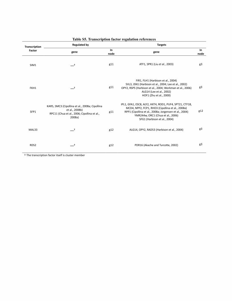
Table S5. Transcription factor regulation references
Transcription Factor
Regulated by Targets
gene In
node gene
In node
SIM1 † g11 ATF1, SPR1 (Liu et al., 2003) g3
FKH1 † g11
FIR1, FLH1 (Harbison et al., 2004) SVL3, JSN1 (Harbison et al., 2004; Lee et al., 2002)
OPY2, RSP5 (Harbison et al., 2004; Workman et al., 2006) ALG14 (Lee et al., 2002) HOF1 (Zhu et al., 2000)
g3
SFP1
KAR5, SMC3 (Cipollina et al., 2008a; Cipollina et al., 2008b)
RPC11 (Chua et al., 2006; Cipollina et al., 2008a)
g11
IPL1, GFA1, ESC8, ALY2, HXT4, ROD1, PUF4, SPT21, CTF18, MCD4, NPP2, FCP1, RHO3 (Cipollina et al., 2008a)
RPP1 (Cipollina et al., 2008a; Jorgensen et al., 2004) YMR244w, ORC1 (Chua et al., 2006)
SFG1 (Harbison et al., 2004)
g12
MAL33 † g12 ALG14, OPY2, RAD53 (Harbison et al., 2004) g3
RDS2 † g12 PDR16 (Akache and Turcotte, 2002) g3
† The transcription factor itself is cluster member
References:
Akache, B. and Turcotte, B. (2002) New regulators of drug sensitivity in the family of yeast zinc cluster proteins, J Biol Chem, 277, 21254-21260.
Aoki-Kinoshita, K.F. and Kanehisa, M. (2007) Gene annotation and pathway mapping in KEGG, Methods Mol Biol, 396, 71-91.
Bader, G.D. et al. (2003) BIND: the Biomolecular Interaction Network Database, Nucleic Acids Res, 31, 248--250.
Bader, G.D. and Hogue, C.W. (2000) BIND--a data specification for storing and describing biomolecular interactions, molecular complexes and pathways, Bioinformatics, 16,
465-477.
Bar-Joseph, Z. et al. (2003) Continuous representations of time-series gene expression data, J Comput Biol, 10, 341--356.
Barrett, T. et al. (2009) NCBI GEO: archive for high-throughput functional genomic data, Nucleic Acids Res, 37, D885--D890.
Benjamini, Y. and Hochberg, Y. (1995) Controlling the false discovery rate: a practical and powerful approach to multiple testing, J. R. Stat. Soc. Ser. B, 57, 289–300.
Breitkreutz, B.J. et al. (2008) The BioGRID Interaction Database: 2008 update, Nucleic Acids Res, 36, D637-640.
Cao, K.-A.L. et al. (2008) A sparse PLS for variable selection when integrating omics data, Stat Appl Genet Mol Biol, 7, Article 35.
Chatr-aryamontri, A. et al. (2007) MINT: the Molecular INTeraction database, Nucleic Acids Res, 35, D572-574.
Chua, G. et al. (2006) Identifying transcription factor functions and targets by phenotypic activation, Proc Natl Acad Sci U S A, 103, 12045-12050.
Cipollina, C. et al. (2008a) Saccharomyces cerevisiae SFP1: at the crossroads of central metabolism and ribosome biogenesis, Microbiology, 154, 1686-1699.
Cipollina, C. et al. (2008b) Revisiting the role of yeast Sfp1 in ribosome biogenesis and cell size control: a chemostat study, Microbiology, 154, 337-346.
Culhane, A.C. et al. (2003) Cross-platform comparison and visualisation of gene expression data using co-inertia analysis, BMC Bioinformatics, 4, 59.
Dolédec, S. and Chessel, D. (1994) Co-inertia analysis: an alternative method for studying species-environment relationships, Freshwater Biology, 31, 277-294.
Dray, S. et al. (2003) Procrustean co-inertia analysis for the linking of multivariate data sets, Ecoscience, 10(1), 110-119.
Fagan, A.s. et al. (2007) A multivariate analysis approach to the integration of proteomic and gene expression data, Proteomics, 7, 2162--2171.
Futschik, M.E. and Herzel, H. (2008) Are we overestimating the number of cell-cycling genes? The impact of background models on time-series analysis, Bioinformatics, 24,
1063--1069.
Gittins, R. (1985) Canonical analysis, a review with applications in ecology, Biomathematics, 12.
Guldener, U. et al. (2006) MPact: the MIPS protein interaction resource on yeast, Nucleic Acids Res, 34, D436-441.
Harbison, C.T. et al. (2004) Transcriptional regulatory code of a eukaryotic genome, Nature, 431, 99-104.
Hermjakob, H. et al. (2004) IntAct: an open source molecular interaction database, Nucleic Acids Res, 32, D452--D455.
Huber, W. et al. (2002) Variance stabilization applied to microarray data calibration and to the quantification of differential expression, Bioinformatics, 18 Suppl 1, S96--104.
Jeffery, I.B. et al. (2007) Integrating transcription factor binding site information with gene expression datasets, Bioinformatics, 23, 298-305.
Jorgensen, P. et al. (2004) A dynamic transcriptional network communicates growth potential to ribosome synthesis and critical cell size, Genes Dev, 18, 2491-2505.
Kanehisa, M. et al. (2008) KEGG for linking genomes to life and the environment, Nucleic Acids Res, 36, D480--D484.
Kerrien, S. et al. (2007) IntAct--open source resource for molecular interaction data, Nucleic Acids Res, 35, D561-565.
Lee, T.I. et al. (2002) Transcriptional regulatory networks in Saccharomyces cerevisiae, Science, 298, 799-804.
Liu, C. et al. (2003) Identification of the downstream targets of SIM1 and ARNT2, a pair of transcription factors essential for neuroendocrine cell differentiation, J Biol Chem,
278, 44857-44867.
Mewes, H.W. et al. (2006) MIPS: analysis and annotation of proteins from whole genomes in 2005, Nucleic Acids Res, 34, D169-172.
Moggs, J.G. et al. (2004) Phenotypic anchoring of gene expression changes during estrogen-induced uterine growth, Environ Health Perspect, 112, 1589-1606.
Oliva, A. et al. (2005) The cell cycle-regulated genes of Schizosaccharomyces pombe, PLoS Biol, 3, e225.
Parkhomenko, E. et al. (2009) Sparse canonical correlation analysis with application to genomic data integration, Stat Appl Genet Mol Biol, 8, Article1.
Parkinson, H. et al. (2009) ArrayExpress update--from an archive of functional genomics experiments to the atlas of gene expression, Nucleic Acids Res, 37, D868--D872.
Rustici, G. et al. (2004) Periodic gene expression program of the fission yeast cell cycle, Nat Genet, 36, 809--817.
Singh, A.V. et al. (2007) Integrative analysis of the mouse embryonic transcriptome, Bioinformation, 1, 406-413.
Smyth, G.K. (2004) Linear models and empirical bayes methods for assessing differential expression in microarray experiments, Stat Appl Genet Mol Biol, 3, Article3.
Stark, C. et al. (2006) BioGRID: a general repository for interaction datasets, Nucleic Acids Res, 34, D535--D539.
Stossi, F. et al. (2004) Transcriptional profiling of estrogen-regulated gene expression via estrogen receptor (ER) alpha or ERbeta in human osteosarcoma cells: distinct and com-
mon target genes for these receptors, Endocrinology, 145, 3473-3486.
Thioulouse, J. and Lobry, J.R. (1995) Co-inertia analysis of amino-acid physico-chemical properties and protein composition with the ADE package, Comput Appl Biosci, 11, 321-
-329.
Troyanskaya, O. et al. (2001) Missing value estimation methods for DNA microarrays, Bioinformatics, 17, 520--525.
Waaijenborg, S. et al. (2008) Quantifying the association between gene expressions and DNA-markers by penalized canonical correlation analysis, Stat Appl Genet Mol Biol, 7,
Article3.
Willis, R.C. and Hogue, C.W. (2006) Searching, viewing, and visualizing data in the Biomolecular Interaction Network Database (BIND), Curr Protoc Bioinformatics, Chapter 8,
Unit 8 9.
Wold, H. (1966) Multivariate Analysis. Academic Press, New York.

Workman, C.T. et al. (2006) A systems approach to mapping DNA damage response pathways, Science, 312, 1054-1059.
Xenarios, I. et al. (2002) DIP, the Database of Interacting Proteins: a research tool for studying cellular networks of protein interactions, Nucleic Acids Res, 30, 303-305.
Zanzoni, A. et al. (2002) MINT: a Molecular INTeraction database, FEBS Lett, 513, 135--140.
Zhu, G. et al. (2000) Two yeast forkhead genes regulate the cell cycle and pseudohyphal growth, Nature, 406, 90-94.
Related Documents