General rights Copyright and moral rights for the publications made accessible in the public portal are retained by the authors and/or other copyright owners and it is a condition of accessing publications that users recognise and abide by the legal requirements associated with these rights. • Users may download and print one copy of any publication from the public portal for the purpose of private study or research. • You may not further distribute the material or use it for any profit-making activity or commercial gain • You may freely distribute the URL identifying the publication in the public portal If you believe that this document breaches copyright please contact us providing details, and we will remove access to the work immediately and investigate your claim. Downloaded from orbit.dtu.dk on: Dec 17, 2017 Decision Support System for Fighter Pilots Randleff, Lars Rosenberg; Clausen, Jens Publication date: 2007 Document Version Publisher's PDF, also known as Version of record Link back to DTU Orbit Citation (APA): Randleff, L. R., & Clausen, J. (2007). Decision Support System for Fighter Pilots. (IMM-PHD-2007-172).

Welcome message from author
This document is posted to help you gain knowledge. Please leave a comment to let me know what you think about it! Share it to your friends and learn new things together.
Transcript

General rights Copyright and moral rights for the publications made accessible in the public portal are retained by the authors and/or other copyright owners and it is a condition of accessing publications that users recognise and abide by the legal requirements associated with these rights.
• Users may download and print one copy of any publication from the public portal for the purpose of private study or research. • You may not further distribute the material or use it for any profit-making activity or commercial gain • You may freely distribute the URL identifying the publication in the public portal
If you believe that this document breaches copyright please contact us providing details, and we will remove access to the work immediately and investigate your claim.
Downloaded from orbit.dtu.dk on: Dec 17, 2017
Decision Support System for Fighter Pilots
Randleff, Lars Rosenberg; Clausen, Jens
Publication date:2007
Document VersionPublisher's PDF, also known as Version of record
Link back to DTU Orbit
Citation (APA):Randleff, L. R., & Clausen, J. (2007). Decision Support System for Fighter Pilots. (IMM-PHD-2007-172).

Decision Support System forFighter Pilots
Lars Rosenberg Randleff
Kongens Lyngby 2007
IMM-PHD-2007-172

Technical University of DenmarkInformatics and Mathematical ModellingBuilding 321, DK-2800 Kongens Lyngby, DenmarkPhone +45 45253351, Fax +45 [email protected]
IMM-PHD: ISSN 0909-3192
Summary
During a mission over enemy territory a fighter aircraft may be engaged byground based threats. The pilot can use different measures to avoid the aircraftfrom being detected by e.g. enemy radar systems. If the enemy detects theaircraft a missile may be fired to seek and destroy the aircraft. Such a missilewill almost always be either radar guided or heat seeking. It will be launchedfrom a permanent launch pad, or it will be man portable and small enoughto fit in the boot of a car. The probability of a missile being detected by on-board sensors depends on the type of missile. If a missile is detected the pilotmay choose to deploy electronic countermeasures to avoid the impact of themissile. The countermeasures to choose depend on e.g. the type of missile andguidance system, distance and direction between the missile and the aircraft,an assessment of the environment hostility, aircraft altitude and airspeed, andthe availability of countermeasures.
Radar systems, guidance of missiles, and electronic countermeasures are all partsof the electronic warfare domain. A brief description of this domain is given.It contains an introduction to both systems working on-board the aircraft andcountermeasures that can be applied to mitigate threats.
This work is concerned with methods for finding proper evasive actions whena fighter aircraft is engaged by ground based threats. To help the pilot indeciding on these actions a decision support system may be implemented. Theenvironment in which such a system must work is described, as are some generalrequirements to the design of the system. Decisions suggested by the system arebased on information acquired from different sources. The process of providinginformation from sources such as intelligence, on-board sensor systems, and
ii
tactical data from other platforms (aircraft, ships, etc.) is described.
Different approaches to finding the combination of countermeasures and ma-noeuvres improving the survivability of the aircraft are investigated. Duringtraining a fighter pilot will learn a set of rules to follow when a threat occurs.For the pilot these rules will be formulated in natural language. An expert sys-tem can be build by translating these rules into a language understandable by acomputer program. This is done in the development of a Prolog based decisionsupport system.
A fighter aircraft decision support system is likely to base its decisions on inputfrom non-perfect sources. Warnings from on-board sensor systems can be falseand intelligence reports deficient. A Bayesian net is modelled to address this.Building the dependency tables of a Bayesian net requires a large number of cellsto be filled with relevant probabilities. Not having sufficient knowledge aboutthese probabilities makes the work with developing a Bayesian net cumbersome.Therefore a method for structural learning is investigated. Here a Bayesian netis build using a set of sample data from a number of missile flight simulations.
Knowledge about threats in the current combat scenario may influence thechoice of evasive manoeuvres and proper countermeasures. If at any given timemore expendable countermeasures are dispensed than necessary, and none is leftfor a later necessity, the survivability of the aircraft may decrease. A mathe-matical model is developed to describe this problem. It is solved to optimalityusing solver software. When new threats occur the decision support systemmust be able to provide suggestions within a fraction of a second. Since thetime it takes to find an optimal solution to the mathematical model can notcomply with this requirement solutions are sought using a metaheuristic.
Resume
Nar et jagerfly flyver over fjendtligt omrade, kan det blive udsat for jordbaseredetrusler. For at undga at blive opdaget af f.eks. fjendtlige radarsystemer, kan pi-loten benytte sig af forskellige modmidler. Er flyet først blivet opdaget, kanfjenden affyre missiler mod det. Sadan et missil vil næsten altid være en-ten radarstyret eller varmesøgende. Det kan blive affyret fra en permanentaffyringsrampe, eller det kan være skulderbarent, og sa lille at det kan skjulesi bagagerummet pa en bil. Sandsynligheden for, at sensorer ombord pa flyetkan detektere missilet afhænger bl.a. af missilets type. Nar et missil er blevetdetekteret, kan piloten vælge at anvende modmidler for at undga, at flyet bliverramt af missilet. Hvilket modmiddel, der skal vælges afhænger bl.a. af mis-siltypen, hvordan missilet er styret, afstand og retning mellem missilet og flyet,en bedømmelse af, hvor fjendtlige omgivelserne er, flyets højde og hastighed ogaf hvilke modmidler der er tilgængelige.
Radarsystemer, styring af missiler og elektroniske modmidler hører alle til idomænet elektronisk krigsførelse. En kort beskrivelse af dette domæne er givether. Beskrivelsen indeholder bade en introduktion til systemer om bord pa flyet,og en beskrivelse af de modmidler, som kan anvedes for at undga missiler.
Arbejdet beskrevet i denne afhandling gar ud pa at finde ud af, hvad pilotenskal foretage sig nar flyet udsættes for jordbaserede trusler. I den forbindelsekan piloten benytte sig af et beslutningsstøttesystem, der kan være installereti jagerflyets cockpit. Bade den kontekst hvori et beslutningsstøttesystem skalfungere, samt generelle krav til designet af systemet er beskrevet. Systemetsbeslutninger vil være baseret pa informationer fra forskellige kilder, og processenmed at fremskaffe informationer fra efterretningskilder, sensorsystemer ombordpa flyet og taktiske data fra andre andre fly, skibe, osv. er kort beskrevet.

iv
Forskellige tilgangsvinkler til det at finde den optimale kombination af mod-midler og manøvrer er blevet undersøgt. En del af det en jagerpilot lærer undersin uddannelse vil kunne sammenfattes i et sæt regler, som skal følges nar jager-flyet møder en trussel. Disse regler kan formuleres i naturligt sprog. Ved atoversætte disse regler til et sprog, der kan forstas af et computerprogram, kanman udvikle et ekspertsystem. Pa denne made er et beslutningsstøttesystembaseret pa sproget Prolog blevet udviklet.
Et beslutningsstøttesystem kan basere sine beslutninger pa data, der ofte vilkomme fra fejlbehæftede kilder. Advarsler fra sensorsystemer ombord pa flyetkan være fejlagtige, og efterretninger kan være mangelfulde. Et bayesiansknet er blevet udviklet for at kunne handtere dette. Afhængighedstabellernei et bayesiansk net skal udfyldes med et stort antal sandsynligheder. Det erbesværligt at udvikle et bayesiansk net bliver, hvis der ikke pa forhand ertilstrækkelig kendskab til disse sandsynligheder. Derfor er en metode til au-tomatisk generering af et bayesiansk net blevet undersøgt, og baseret pa datafra et antal simulerede missilangreb er et net blevet konstrueret.
Valget af manøvrer og modmidler vil afhænge af tilgængelig viden om trusleri det aktuelle scenarie. Hvis der pa et tidspunkt anvendes flere modmidlerend nødvendigt, og der derfor ikke er nok modmidler tilbage, hvis de pa etsenere tidspunkt skulle blive nødvendige, kan dette øge flyets risiko for at bliveskudt ned. En matematisk model er blevet udviklet for at beskrive dette. Etbeslutningsstøttesystem skal kunne give forslag til forbedring af flyets over-levelseschancer i løbet af meget kort tid. Eftersom løsning af den matematiskemodel med en solver tilsyneladende ikke kan leve op til dette tidskrav, søgesmodellen løst ved brug af en metaheuristik.
Preface
This dissertation was prepared at the department of Informatics and Mathe-matical Modelling at the Technical University of Denmark, in partial fulfilmentof the requirements for acquiring the Ph.D. degree.
Both concepts of electronic warfare and the need for a decision support sys-tem in fighter aircraft are described. Such a system must suggest actions tothe fighter pilot that will increase his chances of surviving a mission when fly-ing over enemy territory. For finding these actions four different technologieshave been evaluated. Each of the technologies are described in the dissertation.The technologies are compared with regards to a number of requirements, andrecommendations for further work within this area are made.
Acknowledgements
In November 2003 I began as a Ph.D. student at the Danish Defence ResearchEstablishment (DDRE) with Per Husmann Rasmussen as my supervisor. Perhad many ideas for the Ph.D. project and we spent days together discussingthese. Sadly, Per became seriously ill, and he passed away in the Summer of2004. While supervising this Ph.D. project for a short time only, large parts ofthe work on Bayesian Network (BN) described in this dissertation is still basedon Per’s ideas. During the work with the BN approach I visited Kristian G.Olesen at the Department of Computer Science at the University of Aalborg.Kristian evaluated the model developed and gave hints on improvements of bothstructure and running time.
vi
At DDRE Gert Hvedstrup Jensen took over as my supervisor. Since Gert hasan interest in the use of Prolog this was chosen as the next approach. SteenSøndergaard and Jim Titley took it upon them to introduce me to the frighteningyet fascinating world of Electronic Warfare (EW). They willingly answered allof my more or less cryptic questions about missiles, guidance systems, and stateof the art, and they enthusiastically reviewed all of my ideas.
Part of the work has taken place in the section for Operations Research (OR)at the department of Informatics and Mathematical Modelling at the TechnicalUniversity of Denmark. Here I have had Professor Jens Clausen as my mainsupervisor. Inspired by OR courses taken, and under the advice of Jens, amathematical model has been formulated. This has been done with assistanceof Associate Professor Jesper Larsen.
In the summer of 2005 I had a two month stay at the Georgia Tech ResearchInstitute (GTRI) in Atlanta, Georgia. Here I had a beneficial cooperation withDr. Fred Wright on the formulation of time aspects in a combat mission. HereI also met Lee Simonetta who took time from his busy schedule to escort meto Tucson, Arizona, to Jacksonville, Florida, and to Marietta, Georgia. RandyScott organized my stay at Georgia Tech, and he spent many hours showing memy way around the Georgia Tech campus and on sightseeing all over Atlanta.
All the people mentioned here have helped me in my work with the Ph.D projectand with this dissertation, and I would like to thank them for their efforts. Iwould also like to thank all the people who spend time proof reading this disser-tation. While they have corrected misspelled words, bad wording, and misinter-pretations, the errors remaining are all mine. Thanks also to Henrik Jørgensenfrom Terma for supplying some of the pictures given in this dissertation.
Finally, I would like to thank my family. Both Ane and our son Christianhave suffered from my regular absence, both physically and mentally, since thebeginning of the project. Thanks also to our son Mads, who planned the dateof his arrival so that I could return from Atlanta just before he was born.
Lyngby, March 2007
Lars Rosenberg Randleff

Acronyms and Abbreviations
AAM Air-to-Air Missile
ACS Aircraft CombatSurvivability
AI Artificial Intelligence
ANN Artificial Neural Net
ATRIA Automated ThreatResponse using IntelligentAgents
BN Bayesian Network
BVR Beyond Visual Range
CLP Constraint LogicProgramming
CMAT CountermeasureAssociation Technique
CMOP CountermeasureOptimisation Problem
DDRE Danish Defence ResearchEstablishment
DG Decision Graph
DIRCM Directional InfraredCountermeasures
DSS Decision Support System
ECAP Electronic CombatAdaptive Processor
ECCM Electronic CounterCountermeasures
ECM ElectronicCountermeasures
EM Estimation-Maximization
EO Electro-Optical
EOB Electronic Order of Battle
EPM Electronic ProtectiveMeasures
ESM Electronic SupportMeasures
EU Expected Utility
EW Electronic Warfare
EWMS Electronic WarfareManagement System
viii Contents
GAMS General AlgebraicModeling System
GAPATS General Aviation PilotAdvisory and TrainingSystem
GPS Global Positioning System
GTRI Georgia Tech ResearchInstitute
HDD Heads-Down Display
HUD Heads-Up Display
ICD Interface ControlDocument
IDAS Integrated Defensive AidsSystem
IFF Identification Friend orFoe System
INS Inertial Navigation System
IP Intermediate Point
IPB Intelligence Preparation ofBattlefield
IR Infrared
JPD Joint ProbabilityDistribution
MANPADS Man Portable Air DefenceSystem
MAWS Missile Approach WarningSystem
MCO Missile CountermeasureOptimization
MFD Multi-Function Display
MWS Missile Warning System
OODA Observe, Orient, Decide,Act
OR Operations Research
PVI Pilot-Vehicle Interface
RCS Radar Cross Section
RF Radar Frequency
RWR Radar Warning Receiver
SA Situational Awareness
SAM Surface-to-Air Missile
SL Structural Learning
TRP Threat Response Processor
TTG Time-to-Go
UAV Unmanned Aerial Vehicle
UV Ultraviolet
Contents
Summary i
Resume iii
Preface v
Acronyms and Abbreviations vii
1 Introduction 1
1.1 Contents . . . . . . . . . . . . . . . . . . . . . . . . . . . . . . . . 1
1.2 Readers Prerequisites . . . . . . . . . . . . . . . . . . . . . . . . . 2
2 Electronic Warfare 3
2.1 The Electromagnetic Spectrum . . . . . . . . . . . . . . . . . . . 3
2.2 Mission Scenarios . . . . . . . . . . . . . . . . . . . . . . . . . . . 6
2.3 Threats . . . . . . . . . . . . . . . . . . . . . . . . . . . . . . . . 8
x CONTENTS
2.4 Electronic Support Measures . . . . . . . . . . . . . . . . . . . . 10
2.5 Electronic Countermeasures . . . . . . . . . . . . . . . . . . . . . 13
2.6 Electronic Protective Measures . . . . . . . . . . . . . . . . . . . 18
2.7 The Fighter Aircraft . . . . . . . . . . . . . . . . . . . . . . . . . 18
2.8 Summary . . . . . . . . . . . . . . . . . . . . . . . . . . . . . . . 22
3 Decision Support System in a Fighter Aircraft 23
3.1 Problem Description . . . . . . . . . . . . . . . . . . . . . . . . . 23
3.2 Survivability . . . . . . . . . . . . . . . . . . . . . . . . . . . . . 25
3.3 Design Requirements . . . . . . . . . . . . . . . . . . . . . . . . . 26
3.4 Mission Data Flow . . . . . . . . . . . . . . . . . . . . . . . . . . 27
3.5 System Data Flow . . . . . . . . . . . . . . . . . . . . . . . . . . 29
3.6 Models and Systems . . . . . . . . . . . . . . . . . . . . . . . . . 33
3.7 Summary . . . . . . . . . . . . . . . . . . . . . . . . . . . . . . . 36
4 The Prolog Approach 37
4.1 Motivation . . . . . . . . . . . . . . . . . . . . . . . . . . . . . . 37
4.2 Basic Theory . . . . . . . . . . . . . . . . . . . . . . . . . . . . . 38
4.3 Answering Questions with Prolog . . . . . . . . . . . . . . . . . . 45
4.4 Using Prolog for Decision Support . . . . . . . . . . . . . . . . . 51
4.5 The Prolog Program . . . . . . . . . . . . . . . . . . . . . . . . . 54
4.6 Testing . . . . . . . . . . . . . . . . . . . . . . . . . . . . . . . . 61
4.7 Discussion . . . . . . . . . . . . . . . . . . . . . . . . . . . . . . . 66
CONTENTS xi
4.8 Conclusion . . . . . . . . . . . . . . . . . . . . . . . . . . . . . . 69
5 The Bayesian Network Approach 71
5.1 Motivation . . . . . . . . . . . . . . . . . . . . . . . . . . . . . . 72
5.2 Basic Theory . . . . . . . . . . . . . . . . . . . . . . . . . . . . . 72
5.3 Building the Model . . . . . . . . . . . . . . . . . . . . . . . . . . 86
5.4 Populating Dependency Tables . . . . . . . . . . . . . . . . . . . 90
5.5 Structural Learning . . . . . . . . . . . . . . . . . . . . . . . . . . 92
5.6 Generating Data with Fly-In . . . . . . . . . . . . . . . . . . . . 98
5.7 Testing . . . . . . . . . . . . . . . . . . . . . . . . . . . . . . . . 100
5.8 Discussion . . . . . . . . . . . . . . . . . . . . . . . . . . . . . . . 105
5.9 Conclusion . . . . . . . . . . . . . . . . . . . . . . . . . . . . . . 107
6 The Mathematical Modelling Approach 109
6.1 Motivation . . . . . . . . . . . . . . . . . . . . . . . . . . . . . . 110
6.2 Linear Programming . . . . . . . . . . . . . . . . . . . . . . . . . 110
6.3 The Framework . . . . . . . . . . . . . . . . . . . . . . . . . . . . 116
6.4 Optimise Survivability . . . . . . . . . . . . . . . . . . . . . . . . 119
6.5 Modelling the Problem . . . . . . . . . . . . . . . . . . . . . . . . 127
6.6 The GAMS Program . . . . . . . . . . . . . . . . . . . . . . . . . 142
6.7 Testing . . . . . . . . . . . . . . . . . . . . . . . . . . . . . . . . 143
6.8 Discussion . . . . . . . . . . . . . . . . . . . . . . . . . . . . . . . 153
6.9 Conclusion . . . . . . . . . . . . . . . . . . . . . . . . . . . . . . 155
xii CONTENTS
7 The Metaheuristics Approach 157
7.1 Motivation . . . . . . . . . . . . . . . . . . . . . . . . . . . . . . 158
7.2 Metaheuristics . . . . . . . . . . . . . . . . . . . . . . . . . . . . 158
7.3 Using Simulated Annealing . . . . . . . . . . . . . . . . . . . . . 164
7.4 Implementing Simulated Annealing . . . . . . . . . . . . . . . . . 171
7.5 Testing . . . . . . . . . . . . . . . . . . . . . . . . . . . . . . . . 179
7.6 Discussion . . . . . . . . . . . . . . . . . . . . . . . . . . . . . . . 181
7.7 Conclusion . . . . . . . . . . . . . . . . . . . . . . . . . . . . . . 184
8 Comparing Approaches 185
8.1 The Approaches . . . . . . . . . . . . . . . . . . . . . . . . . . . 185
8.2 Comparison . . . . . . . . . . . . . . . . . . . . . . . . . . . . . . 192
9 Further Work 195
9.1 Current Approaches . . . . . . . . . . . . . . . . . . . . . . . . . 195
9.2 Testing with Flight Data . . . . . . . . . . . . . . . . . . . . . . . 199
9.3 Other Techniques . . . . . . . . . . . . . . . . . . . . . . . . . . . 201
10 Conclusion 205
A Threats 207
A.1 Guidance Systems . . . . . . . . . . . . . . . . . . . . . . . . . . 207
A.2 Surface-to-Air Missile Reference Guide . . . . . . . . . . . . . . . 211
B The Prolog Program 213
CONTENTS xiii
B.1 Rules . . . . . . . . . . . . . . . . . . . . . . . . . . . . . . . . . . 213
B.2 dss.pro . . . . . . . . . . . . . . . . . . . . . . . . . . . . . . . . 215
B.3 util.pro . . . . . . . . . . . . . . . . . . . . . . . . . . . . . . . 221
B.4 cm.pro . . . . . . . . . . . . . . . . . . . . . . . . . . . . . . . . . 223
B.5 threats.pro . . . . . . . . . . . . . . . . . . . . . . . . . . . . . 225
B.6 mission.pro . . . . . . . . . . . . . . . . . . . . . . . . . . . . . 227
B.7 current.pro . . . . . . . . . . . . . . . . . . . . . . . . . . . . . 227
B.8 warnings.pro . . . . . . . . . . . . . . . . . . . . . . . . . . . . . 228
C Survival Score 229
C.1 Constructing a score system . . . . . . . . . . . . . . . . . . . . . 229
C.2 Optimising the score . . . . . . . . . . . . . . . . . . . . . . . . . 231
C.3 Further work . . . . . . . . . . . . . . . . . . . . . . . . . . . . . 232
D The GAMS Program 233
D.1 tempasp.gms . . . . . . . . . . . . . . . . . . . . . . . . . . . . . 233
E Software and Hardware 241
E.1 Software . . . . . . . . . . . . . . . . . . . . . . . . . . . . . . . . 241
E.2 Hardware . . . . . . . . . . . . . . . . . . . . . . . . . . . . . . . 242

xiv CONTENTS
Chapter 1
Introduction
A fighter aircraft on duty will often fly over enemy territory as part of a mission.During this mission the aircraft may be engaged by enemy aircraft, or it maybe the target of missiles fired from ground based launch pads. Over time moreand more systems have been implemented aboard fighter aircraft in order toimprove the pilot’s awareness about the condition of the aircraft and the cur-rent situation in the world surrounding it. As the number and complexity ofthese systems increase, so does the quantity of threats to the aircraft. Whennew threats emerge, the pilot’s means of mitigating these threats will change.Already known countermeasures may be applied in new and different ways, andnew countermeasures are designed. When threats occur proper evasive actionsoften consist of combinations of manoeuvres and applied countermeasures. Todetermine the proper action, the pilot may benefit from a decision support sys-tem implemented on-board the aircraft.
1.1 Contents
In order to acknowledge the need for a decision support system on-board afighter aircraft one has to understand the kind of threats an aircraft may meet,what type of information on-board sensors may provide to the pilot, and whathe can do to avoid the threats. Most threats, and the relevant countermeasures,
2 Introduction
either receive or emit electromagnetic radiation, and the domain is often referredto as Electronic Warfare (EW). This domain is described in Chapter 2. Theintention with this chapter is to provide the reader with enough understandingabout Electronic Warfare to understand the considerations given in designing adecision support system for fighter pilots.
In Chapter 3 the basics of a decision support system in the realm of electronicwarfare are described. The context of such a system is described and require-ments to the development of the system are specified. Already existing systems,and some academical approaches to designing them, are also described here.
The aim of the work documented in this dissertation is to explore a number ofapproaches to the development of a decision support system for fighter pilots.These approaches comprise Prolog (Chapter 4), Bayesian Networks (Chapter 5),formulating and solving a mathematical integer programming model (Chapter6), and the use of metaheuristics to solve the mathematical model in due time(Chapter 7). These four approaches are compared in Chapter 8.
Throughout the dissertation the pilot of the aircraft will, for convenience, bereferred to as he/him. The aircraft described is intended to be generic, andprices for missiles, countermeasures and aircraft, are all fictitious.
1.2 Readers Prerequisites
The intended reader of this thesis should have enough statistical literacy tocomprehend the basics of Bayesian networks. To fully understand the chaptersabout mathematical modelling and metaheuristics, some degree of mathematicalmaturity is needed as well. To understand the brief introduction to logic and theProlog programming language given, the reader will benefit from some experi-ence with programming. Knowledge about fighter aircraft or electronic warfareis not needed, as these issues are covered sufficiently for the understanding of theapproaches described. All sections containing mathematical theory are writtenwithout the use of lemmas, corollaries, and theorems. This is a deliberate choiceto ease reading of these parts of the report. For the proper definitions, theorems,and proofs the reader is encouraged to consult the referenced textbooks.
Chapter 2
Electronic Warfare
A large part of the warfare involving fighter aircraft is based on the use ofelectromagnetic radiation. This type of warfare is referred to as ElectronicWarfare (EW) (also known as Electronic Combat). EW is defined as militaryactions using electromagnetic radiation to estimate, use, reduce, or avoid enemyuse of the electromagnetic spectrum.
The EW taxonomy can be divided into three main parts: Electronic SupportMeasures (ESM), Electronic Countermeasures (ECM), and Electronic ProtectiveMeasures (EPM). ESM is used to gain knowledge about the enemy using sensorsbased on electromagnetic radiation. To obstruct enemy use of ESM ECM isused. Finally EPM is used to lower the applicability of the enemy’s use of ECM.Terms within these three classes of EW are described in this chapter. For moredetailed descriptions on these subjects the books [41, 42, 46] are recommended.The threats, sensors, countermeasures, and fighter aircraft described in this andfollowing chapters are all assumed generic.
2.1 The Electromagnetic Spectrum
Electromagnetic radiation is a common description of physical phenomena suchas visible light, X-rays, radar, infrared, and ultraviolet radiation. All of these
4 Electronic Warfare
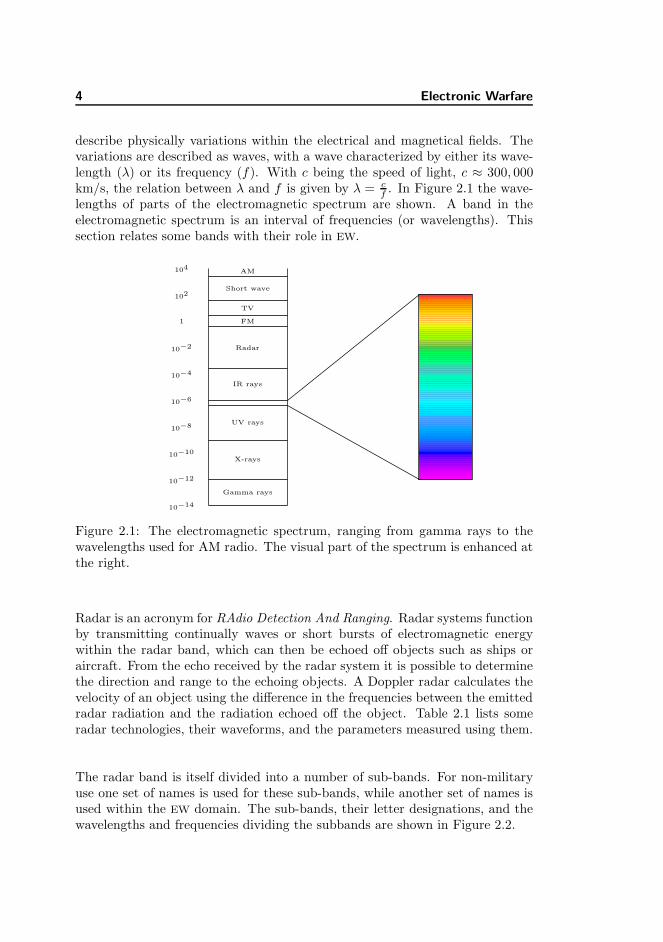
describe physically variations within the electrical and magnetical fields. Thevariations are described as waves, with a wave characterized by either its wave-length (λ) or its frequency (f). With c being the speed of light, c ≈ 300, 000km/s, the relation between λ and f is given by λ = c
f . In Figure 2.1 the wave-lengths of parts of the electromagnetic spectrum are shown. A band in theelectromagnetic spectrum is an interval of frequencies (or wavelengths). Thissection relates some bands with their role in EW.
AM
Short wave
TV
FM
Radar
IR rays
UV rays
X-rays
Gamma rays
104
102
1
10−2
10−4
10−6
10−8
10−10
10−12
10−14
Figure 2.1: The electromagnetic spectrum, ranging from gamma rays to thewavelengths used for AM radio. The visual part of the spectrum is enhanced atthe right.
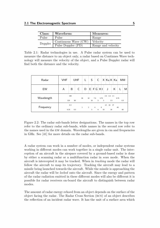
Radar is an acronym for RAdio Detection And Ranging. Radar systems functionby transmitting continually waves or short bursts of electromagnetic energywithin the radar band, which can then be echoed off objects such as ships oraircraft. From the echo received by the radar system it is possible to determinethe direction and range to the echoing objects. A Doppler radar calculates thevelocity of an object using the difference in the frequencies between the emittedradar radiation and the radiation echoed off the object. Table 2.1 lists someradar technologies, their waveforms, and the parameters measured using them.
The radar band is itself divided into a number of sub-bands. For non-militaryuse one set of names is used for these sub-bands, while another set of names isused within the EW domain. The sub-bands, their letter designations, and thewavelengths and frequencies dividing the subbands are shown in Figure 2.2.
2.1 The Electromagnetic Spectrum 5
Class: Waveform: Measures:Pulse Pulse Range
DopplerContinuous Wave (CW) VelocityPulse Doppler (PD) Range and velocity
Table 2.1: Radar technologies in use. A Pulse radar system can be used tomeasure the distance to an object only, a radar based on Continues Wave tech-nology will measure the velocity of the object, and a Pulse Doppler radar willfind both the distance and the velocity.
Radar
EW
Wavelength
Frequency
VHF UHF L S C X Ku K Ka MM
A B C D E F G H I J K L M
120
100
80
30 15
10
7.5
5
3.75
3
2.5 1.6
1.5
1.1
0.75
0.5
0.25
0.3
0.5
1 2
3
4
6
8
10
12 18
20
27
40
60
Figure 2.2: The radar sub-bands letter designations. The names in the top rowrefer to the ordinary radar sub-bands, while names in the second row refer tothe names used in the EW domain. Wavelengths are given in cm and frequenciesin GHz. See [41] for more details on the radar sub-bands.
A radar system can work in a number of modes, or independent radar systemsworking in different modes can work together in a single radar unit. The inter-ception of an aircraft in the airspace covered by a ground-based radar is doneby either a scanning radar or a multifunction radar in scan mode. When theaircraft is intercepted it may be tracked. When in tracking mode the radar willfollow the aircraft to map its trajectory. Tracking the aircraft may lead to amissile being launched towards the aircraft. While the missile is approaching theaircraft the radar will be locked onto the aircraft. Since the energy and patternof the radar radiation emitted in these different modes will also be different it ispossible for radar receivers on-board the aircraft to distinguish between radarmodes.
The amount of radar energy echoed from an object depends on the surface of theobject facing the radar. The Radar Cross Section (RCS) of an object describesthe reflection of an incident radar wave. It has the unit of a surface area which
6 Electronic Warfare
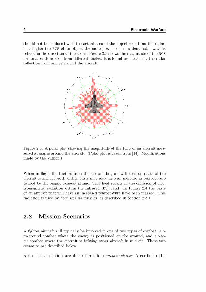
should not be confused with the actual area of the object seen from the radar.The higher the RCS of an object the more power of an incident radar wave isechoed in the direction of the radar. Figure 2.3 shows the magnitude of the RCS
for an aircraft as seen from different angles. It is found by measuring the radarreflection from angles around the aircraft.
Figure 2.3: A polar plot showing the magnitude of the RCS of an aircraft mea-sured at angles around the aircraft. (Polar plot is taken from [14]. Modificationsmade by the author.)
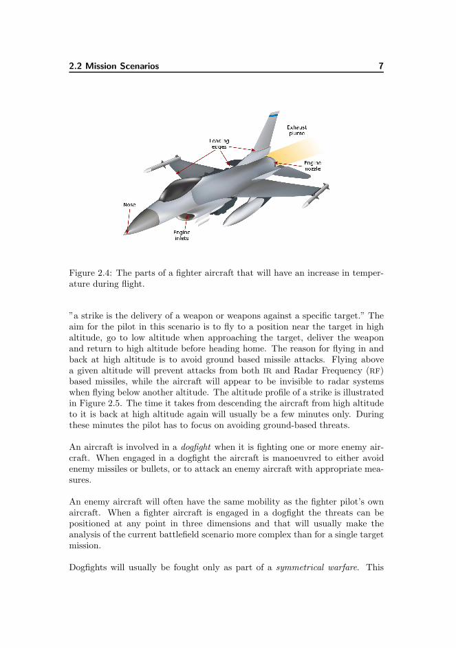
When in flight the friction from the surrounding air will heat up parts of theaircraft facing forward. Other parts may also have an increase in temperaturecaused by the engine exhaust plume. This heat results in the emission of elec-tromagnetic radiation within the Infrared (IR) band. In Figure 2.4 the partsof an aircraft that will have an increased temperature have been marked. Thisradiation is used by heat seeking missiles, as described in Section 2.3.1.
2.2 Mission Scenarios
A fighter aircraft will typically be involved in one of two types of combat: air-to-ground combat where the enemy is positioned on the ground, and air-to-air combat where the aircraft is fighting other aircraft in mid-air. These twoscenarios are described below.
Air-to-surface missions are often referred to as raids or strikes. According to [10]
2.2 Mission Scenarios 7
Figure 2.4: The parts of a fighter aircraft that will have an increase in temper-ature during flight.
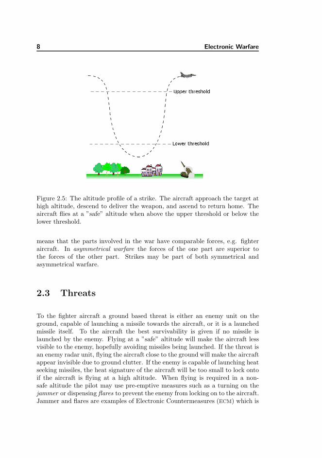
”a strike is the delivery of a weapon or weapons against a specific target.” Theaim for the pilot in this scenario is to fly to a position near the target in highaltitude, go to low altitude when approaching the target, deliver the weaponand return to high altitude before heading home. The reason for flying in andback at high altitude is to avoid ground based missile attacks. Flying abovea given altitude will prevent attacks from both IR and Radar Frequency (RF)based missiles, while the aircraft will appear to be invisible to radar systemswhen flying below another altitude. The altitude profile of a strike is illustratedin Figure 2.5. The time it takes from descending the aircraft from high altitudeto it is back at high altitude again will usually be a few minutes only. Duringthese minutes the pilot has to focus on avoiding ground-based threats.
An aircraft is involved in a dogfight when it is fighting one or more enemy air-craft. When engaged in a dogfight the aircraft is manoeuvred to either avoidenemy missiles or bullets, or to attack an enemy aircraft with appropriate mea-sures.
An enemy aircraft will often have the same mobility as the fighter pilot’s ownaircraft. When a fighter aircraft is engaged in a dogfight the threats can bepositioned at any point in three dimensions and that will usually make theanalysis of the current battlefield scenario more complex than for a single targetmission.
Dogfights will usually be fought only as part of a symmetrical warfare. This
8 Electronic Warfare
Figure 2.5: The altitude profile of a strike. The aircraft approach the target athigh altitude, descend to deliver the weapon, and ascend to return home. Theaircraft flies at a ”safe” altitude when above the upper threshold or below thelower threshold.
means that the parts involved in the war have comparable forces, e.g. fighteraircraft. In asymmetrical warfare the forces of the one part are superior tothe forces of the other part. Strikes may be part of both symmetrical andasymmetrical warfare.
2.3 Threats
To the fighter aircraft a ground based threat is either an enemy unit on theground, capable of launching a missile towards the aircraft, or it is a launchedmissile itself. To the aircraft the best survivability is given if no missile islaunched by the enemy. Flying at a ”safe” altitude will make the aircraft lessvisible to the enemy, hopefully avoiding missiles being launched. If the threat isan enemy radar unit, flying the aircraft close to the ground will make the aircraftappear invisible due to ground clutter. If the enemy is capable of launching heatseeking missiles, the heat signature of the aircraft will be too small to lock ontoif the aircraft is flying at a high altitude. When flying is required in a non-safe altitude the pilot may use pre-emptive measures such as a turning on thejammer or dispensing flares to prevent the enemy from locking on to the aircraft.Jammer and flares are examples of Electronic Countermeasures (ECM) which is
2.3 Threats 9
described in Section 2.5.
According to [6] about 650 different missile systems have been developed, and itis believed that 200-300 of these are still deployed1. A missile launched againstan aircraft will be fired from either the surface of the earth (a Surface-to-AirMissile (SAM)) or from another aircraft (an Air-to-Air Missile (AAM)). Besideshaving a name given by the manufacturer many missile types are also given aUSA/NATO type name, indicating the use of the missile. An example of thisis the Russian S-75 Dvina/Volkhov that has the USA/NATO type name SA-2,indicating that it is a surface-to-air missile.
Some types of missiles are associated with one or more types of radar systems.Therefore the pilot may know which type of missile he is likely to encounterwhen knowledge about the type of a detected enemy radar system has beenestablished. Knowing the missile type may give the pilot knowledge about howthe missile can be countered. Since heat seeking missiles are not associated witha radar system, the pilot will not have this advantage when such a missile islaunched.
For many types of missiles a direct hit at the aircraft is not necessary for itto have an impact. Many missiles are supplied with proximity fuses which willmake the missile go off when it is within a certain range of the aircraft.
2.3.1 Guidance
Most missiles use some form of guidance in directing the missile towards thetarget. To avoid an incoming missile the pilot has to ”break” the guidance(break lock), or transfer it from the aircraft to another object (lock transfer).
The guidance systems generally use electromagnetic radiation within one of twobands: Radar Frequency (RF) or Infrared (IR). If the missile is RF guided it iseither equipped with a radar system of its own, or it is guided by a ground-basedradar system. RF based missile guidance is active since it is based on emittingelectromagnetic radiation to determine the position of the aircraft. When radarradiation is emitted from either the missile or from ground-based radar it maybe detected by the aircraft, thus warning the pilot about an attack.
The IR based missile guidance is passive since it depends solely on radiationemitted from the aircraft and does not emit radiation itself. This type of missilesare equipped with an IR sensitive sensor that will guide the missile towards the
1As of February 2007.
10 Electronic Warfare
aircraft. More sophisticated guidance systems are equipped with IR camerasthat feed images to a seeker algorithm. This algorithm analyses the IR imagesto detect the aircraft and to distinguish it from false targets. The false targetsmay originate from objects in the scenario such as radiation from the sun orsparks from a welding unit, or they may be artificial targets created by theaircraft (see Section 2.5.3). A number of guidance systems are described inAppendix A.1.
As a rule of thumb the more energy that is emitted from or echoed off an objectin the direction of a guidance system, the easier it is for the guidance system tofollow the object. The pilot may manoeuvre the aircraft to reduce the amountof energy that is emitted towards an enemy observer. See Section 2.5.7 for adescription of breaklock zones.
In many situations IR guided missiles, such as the Man Portable Air DefenceSystem (MANPADS), will be the enemy’s best choice of weapon. Often systemsfor launching these missiles are cheaper than systems using RF guidance, theyare small enough to be stored in the boot of a car, they can be operated withlittle training, and until launched they are not easily detectable from the aircraft.Usually the missiles are launched when the distance to the aircraft is less thana few kilometres which will give the pilot only a few seconds to perform evasiveactions. For these reasons IR guided missiles are often considered the greatestthreat to both military and civilian aviation.
2.4 Electronic Support Measures
Equipment working within the electromagnetic spectrum to make the pilotaware of the combat situation surrounding the aircraft are known as ElectronicSupport Measures (ESM). The pilot bases his Situational Awareness (SA) on theESM on-board the aircraft, and the better equipped the aircraft is, the betterSA the pilot may obtain. In this section some of these measures are described.
2.4.1 Radar Warning Receiver
Different types of radar systems have different characteristics, and this is usedby the Radar Warning Receiver (RWR) to determine from which type of radarsystem incoming radar waves originate. This is done by finding the propertiesof the wave in a lookup table. In this table the kind of missile often associatedwith the radar system may also be found. Based on the table a warning symbol
2.4 Electronic Support Measures 11
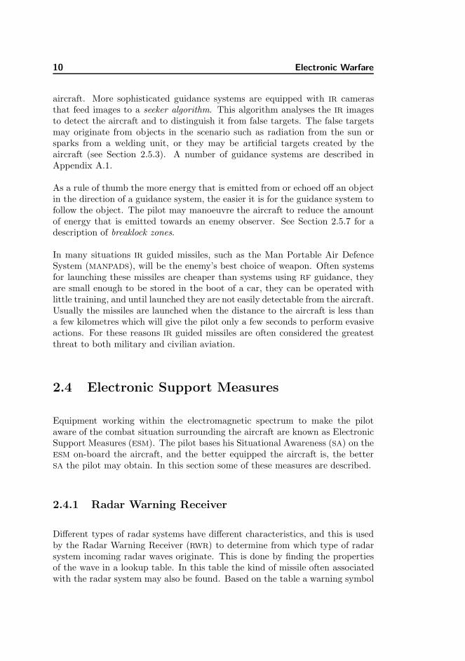
is shown in the azimuth indicator, and an audio warning is given to the pilot.The symbol displayed on the azimuth indicator shows the type of the radarsystem and the direction towards it. If the RWR can not show the type of radarsystem related to the detected radar signal, the azimuth indicator will indicatethe radar system as being of an unknown type. Appendix A describes some ofthe RF-based threats detectable by a RWR. An azimuth indicator is shown inFigure 2.6.
Figure 2.6: An azimuth indicator as part of the Advanced Threat Display.(Photo courtesy of Terma.)
The position of a symbol shown in the azimuth indicator indicates the angletowards the threat and the proximity to the lethal envelope of the threat. Thelethal envelope is the range in which the threat can engage the aircraft, and if theaircraft is close to, or within, the range of a threat this is shown in the azimuthindicator. For some azimuth indicators the symbols closest to the centre willrepresent the most imminent threats, while others will have these farthest awayfrom the centre. While the first of these may seem most intuitive, the latter hasits advantages. It will allow greater spatial separation of the highest prioritythreats on the display, making it easier for the pilot to determine directions tothreats.
Usually the aircraft will be detected by enemy search radar before it is beingtracked or locked upon. Radar characteristics vary from search radar to trackingradar and the RWR on-board the aircraft is able to distinguish between theseradar modes based on the characteristics of incoming radar radiation. It is worthnoting that not all symbols shown in the azimuth indicator represent threats.In any given scenario there may be numerous radars present, and possibly noneor only a few of these represent a threat. Symbols representing search radarsand acquisition and tracking radars may all be displayed simultaneously on the
12 Electronic Warfare
azimuth indicator. Most newer RWR systems offer the possibility of prioritizingthe threats and showing symbols for the threats with the highest priority only.Older RWR systems will only show the symbols of tracking radars and launchedmissiles.
2.4.2 Missile Warning System
The Missile Warning System (MWS) (sometimes referred to as Missile ApproachWarning System (MAWS)) informs the pilot when a missile is approaching theaircraft. In a passive IR based MWS this is detected by continuously analysing IR
images of the aircraft surroundings. These images are acquired using on-boardIR sensors or IR cameras. If the images contain a hot spot (possibly indicatingthe plume of an approaching missile) that increases in size over a relatively shorttime span and which seems to follow the aircraft, a missile warning is issued.
In a passive Ultraviolet (UV) based MWS the images analysed are showing in-formation from the UV part of the electromagnetic spectrum. This type of MWS
has some benefits compared to the IR-based MWS since the UV characteristicsof a missile plume may change during its flight. Information about the missile(time since launch, time to burn out, etc.) may then be extracted from the UV
images.
A RF based MWS is an active system working in the radar band. It can de-termine the range and velocity of an approaching missile, thus giving the pilotan estimate of the time left before the aircraft is hit, known as the Time-to-Go (TTG). This helps the pilot to find the best point in time for performingevasive actions. A drawback to this kind of MWS is that missiles may be veryhard to detect due to small RCS values. Another drawback is that missiles maybe designed to follow the emitted radar radiation thus unfortunately convertingthe MWS into a missile attraction system.
2.4.3 Identification Friend or Foe
In a complex battle scene with many military platforms, including aircraft,ships, and/or ground-based vehicles, it might be difficult for the pilot to tellfriend from foe. To help this the vehicles may be equipped with transpondersidentifying themselves. An aircraft equipped with an Identification Friend orFoe System (IFF) can then detect the transponder signal and it will identify thetransponding vehicle as ”friend” or ”foe”. Since not all aircraft are equippedwith an IFF transponder, or a given transponder may not be turned on, the
2.5 Electronic Countermeasures 13
pilot may not assume other aircraft not identifying themselves as ”friends” tobe, by default, ”foes”.
As with the RF based MWS a transponding IFF system will give away the positionof the aircraft and it must be switched off if the presence of the aircraft is to behidden from the enemy.
2.5 Electronic Countermeasures
The ESM onboard an aircraft continually informs the pilot about enemy threats.For the aircraft to counter these threats the aircraft may be equipped witha number of Electronic Countermeasures (ECM). These measures are used toeither tell the pilot about the ESM used by the enemy, to disrupt the enemy’susage of his ESM, or a combination of both.
2.5.1 Jammer
A radar system will usually analyse the radar signals echoed off an aircraft.Depending on the type of radar system this analysis will decide the velocity,range, and/or direction to the aircraft. The results of this analysis might beused by the ground-based radars to determine when a missile must be launchedagainst an aircraft. To confuse the analysis made by the radar system theaircraft can be equipped with a radar jammer. Different types of jammers exist:the simplest ones jams the radar signal by emitting a noise signal in the samefrequency band as that of the radar signal. More advanced jammers calculatewhat radar signal to send out to make the results of the analysis in the receivingradar system erroneous, e.g. by estimating a wrong velocity, range, or angle.This may e.g. delude the radar into observing the aircraft as approaching whileit may in fact be keeping its distance or even increasing it.
For a jammer to be effective against enemy radars the jamming signal needs tobe emitted using more power than that of the echoed radar signal. Doing thiswill make the enemy radar interpret the actually echoed signal as noise comparedto the jamming signal. The difference in power between the jammer signal andthe echoed radiation is being used by some missile guidance systems. These willguide missiles towards any high-power signal, regardless of the information thatmay be found analysing this signal. A jammer that is turned on will thus serveas a beacon, possibly attracting the attention of an enemy radar operator. Itit is therefore advisable to keep any jamming equipment turned off unless it is
14 Electronic Warfare
considered necessary for the survival of the pilot to have it turned on.
2.5.2 Chaff
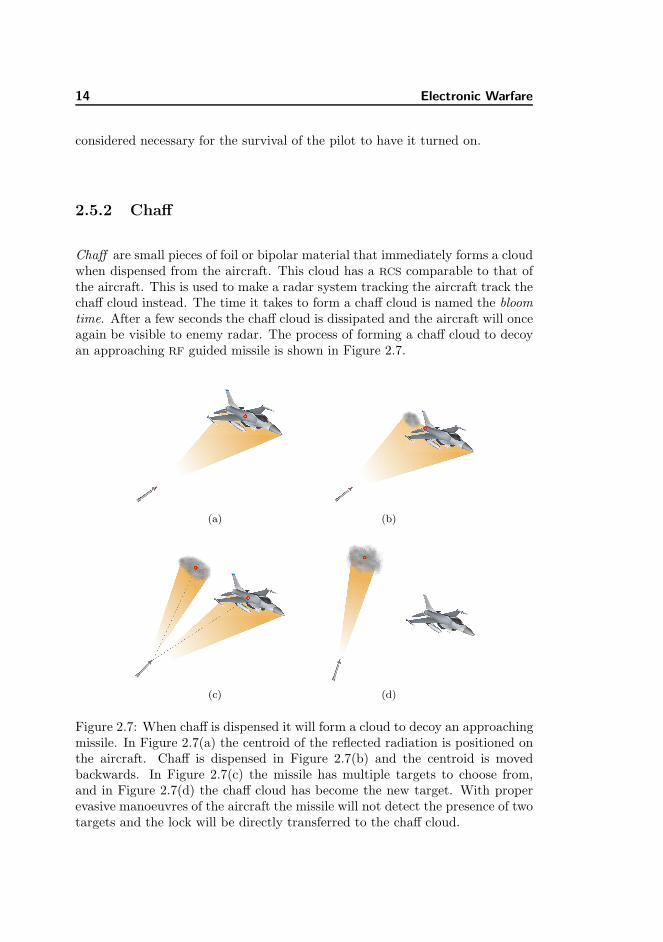
Chaff are small pieces of foil or bipolar material that immediately forms a cloudwhen dispensed from the aircraft. This cloud has a RCS comparable to that ofthe aircraft. This is used to make a radar system tracking the aircraft track thechaff cloud instead. The time it takes to form a chaff cloud is named the bloomtime. After a few seconds the chaff cloud is dissipated and the aircraft will onceagain be visible to enemy radar. The process of forming a chaff cloud to decoyan approaching RF guided missile is shown in Figure 2.7.
(a) (b)
(c) (d)
Figure 2.7: When chaff is dispensed it will form a cloud to decoy an approachingmissile. In Figure 2.7(a) the centroid of the reflected radiation is positioned onthe aircraft. Chaff is dispensed in Figure 2.7(b) and the centroid is movedbackwards. In Figure 2.7(c) the missile has multiple targets to choose from,and in Figure 2.7(d) the chaff cloud has become the new target. With properevasive manoeuvres of the aircraft the missile will not detect the presence of twotargets and the lock will be directly transferred to the chaff cloud.
2.5 Electronic Countermeasures 15
The tracking radar will follow an object within a given range gate only. If theaircraft can escape the range gate before the chaff cloud is dissipated it can notbe tracked by the enemy radar before a new acquisition is performed.
The aircraft may be equipped with a number of chaff types and chaff dispensers.These will depend on a description of the battlefield and they are installed duringthe preparation of the aircraft. Chaff is an expendable countermeasure in thatit can only be used for a limited amount of times before the inventory runs dry.
2.5.3 Flares
To escape from an IR guided missile the pilot may have to transfer the missilelock onto another object. This may be done by dispensing flares. Flares areanother type of expendables which are made of hot burning material that formsan infrared signature which can be more attractive for the missile to followthan that of the aircraft. If the guidance system is designed to manoeuvre themissile towards the hottest spot within the visual range it might go for the flaresinstead of the aircraft. Although flares burn out within a few seconds this mightbe enough for the pilot to manoeuvre the aircraft away from the path of themissile.
When flares are dispensed they will soon get a speed remarkably smaller thanthat of the aircraft. The decrease in speed may be a signal to guided missilesthat the object to follow (the aircraft) is not the object currently in focus (aflare). For flares to maintain the same speed as the aircraft they can be eithertethered or self-propelled. Tethered flares are towed behind the aircraft at afixed distance for a while, thus having the same speed as the aircraft itself.Propelled flares will start off by having the same speed as the aircraft. Theywill slowly decrease their speed, and the distance to the aircraft will increase.
If the pilot expects to be engaged by IR guided missiles, flares may be usedpre-emptively. If numerous flares are dispensed before a missile is launched themissile may fail to acquire a lock on the aircraft itself.
As with chaff the number of flares and flare dispensers may vary according to adescription of the battlefield and they will be set during the preparation of theaircraft as well. Flare dispensers may be directly linked to a MWS so a warningof an approaching missile immediately will trigger a flare dispense.
16 Electronic Warfare
2.5.4 Directed Infrared Countermeasure
The Directional Infrared Countermeasures (DIRCM) is a system designed toprotect the aircraft from IR guided missiles. When an approaching missile isdetected by a MWS the DIRCM is directed towards the missile. When active theDIRCM uses pulses of IR energy to jam the IR seekers guiding the missile. Thepulses of IR energy will generally have one of two effects: either the seeker isblinded and will loose focus on the aircraft long enough for the aircraft to breakthe lock, or it will mimic a thermal signature as that of the sun, thus forcing theseeker to look for alternative targets [1]. If the use of IR pulses is accompaniedby the dispense of flares these may serve as new targets for the seeker and thelock is transferred.
2.5.5 Towed Decoy
As mentioned in Section 2.5.1 missiles may be guided toward an active jammer.To avoid this type of missiles while maintaining the effect of a jammer thejammer may be placed in a towed decoy. When deploying a towed decoy a wireconnecting the decoy to the aircraft is unreeled and the decoy will be towedbehind the aircraft at a fixed distance. When the towed decoy is no longerneeded the wire may be re-reeled or simply severed.
The simplest towed decoys will have their own power supply and they willcontinue to jam for as long as the power permits. More sophisticated decoysmay be connected to power supply and sensors on-board the aircraft. They willbe able to adjust the jamming to the current battlefield scenario and they willcontinue to jam for as long as it is deemed necessary.
A towed decoy is kept at a safe distance behind the aircraft. At this distancean impact on the decoy by a missile will leave the aircraft undamaged. Theaircraft manoeuvrability is limited when a towed decoy is deployed, so whenit is no longer in use it must be severed or re-reeled. Before being deployeda towed decoy is usually placed under the aircraft fuselage or under either orboth of the wings. This limits the total number of towed decoys to be deployedduring a mission to one (the fuselage), two (both wings), or three (fuselage andwings).
2.5 Electronic Countermeasures 17
2.5.6 Stealth
The highest survivability for the aircraft is obtained if it can fly by stealth, i.e.fly without being observed by the enemy. In designing a fighter aircraft severalmeasures are taken to reduce the signatures of the aircraft to make it difficult forthe enemy to observe. These measures include using radar absorbing materialsand shaping the surface of the aircraft to obtain the smallest RCS values possible.A reduction of the IR signature of the aircraft is obtained by special designs ofthe airframe and propulsion system [10].
2.5.7 Breaklock Zones
The signatures of a fighter aircraft influence the success of an approaching mis-sile. If the RCS of the aircraft is sufficiently small a RF guided missile will not beable to lock onto it. Likewise, an IR guided missile will have trouble following anaircraft that is almost invisible within the IR band. During flight the pilot willmanoeuvre the aircraft to obtain the smallest signatures possible. An aircraftwill typically have the largest RCS when seen from the side, while the RCS isoften smallest when the aircraft is flying directly towards the radar receiver. Tolower the IR signature of the aircraft the pilot may reduce the thrust and turnthe aircraft so that hot surfaces are hidden by other parts of the aircraft.
The angles in which the aircraft has the lowest visibility to the enemy are knownas breaklock zones. When a missile is locked onto the aircraft the pilot will ma-noeuvre the aircraft so that the enemy will become positioned within a breaklockzone. The manoeuvre will often be accompanied by the dispense of either chaffor flares, depending on the threat, so the lock can be transferred away from theaircraft.
2.5.8 Timing the Use of Countermeasures
When a threat is detected the use of appropriate countermeasures must be timedto gain the best possible protection. If applied too soon the countermeasuremay have no effect, an applied too late the effect may not protect the aircraft.Dispensed too early a chaff cloud will be dissipated before having any effect onthe missile, and the side-effect of having less chaff available will only decreasethe aircraft’s survivability at a later stage. If the chaff is dispensed too latethe effect on the missile will not prevent it from reaching the aircraft. Similarconsiderations must be taken for IR guided missiles and flares. Here the time it

18 Electronic Warfare
takes from launch until the missile reaches the aircraft is usually smaller thanfor RF guided missiles, and flares are usually dispensed as soon as the missilehas been detected.
For on-board countermeasures such as jammer, towed decoy, or DIRCM, thetime it takes before the countermeasure becomes active must be taken intoconsideration. While it may take only a few seconds for the jammer or theDIRCM to settle, or for the towed decoy to be unreeled, the use of these mustbe appropriately timed, just as for expendable countermeasures.
2.6 Electronic Protective Measures
ESM are used by the pilot to gain knowledge about the current battlefield sce-nario, and ECM are used for destroying the enemy’s knowledge about the sce-nario. To spoil the use of ECM by an enemy aircraft one may use ElectronicProtective Measures (EPM) (also known as Electronic Counter Countermeasures(ECCM)). While the descriptions here assume the user of EPM to be a, proba-bly hostile, ground based radar system, EPM may also be applied in a fighteraircraft.
The fighter aircraft may have a RWR to determine the type of an enemy radar,or it may use either an on-board jammer or a towed decoy to deceive the radar.Some radar systems are designed to complicate the analysis done by either theRWR or the jammer. One technology for doing this is frequency agility where theradar system is able to shift the frequency in use. Spread spectrum technologiescan be applied to prevent the aircraft RWR from correctly determine the kindof radar system in use. In spread spectrum the electromagnetic energy will bespread onto a large band within the radar spectrum. This will make the energyin each sub-band seem like background noise and it will be difficult for the RWR
to recognize the radar signal.
2.7 The Fighter Aircraft
The fighter aircraft itself may limit the use of technology within the field of EW.These limits may be set by e.g. the design of the aircraft, the space available foradditional EW equipment, or the manoeuvres required to gain maximum effectof countermeasures. Descriptions of these limits are given in this section.
2.7 The Fighter Aircraft 19
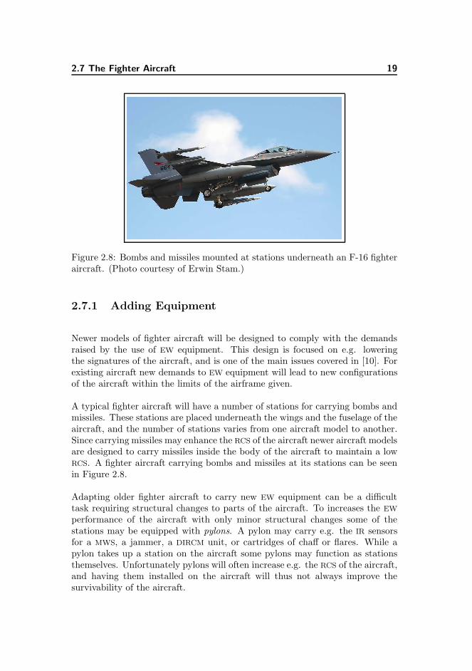
Figure 2.8: Bombs and missiles mounted at stations underneath an F-16 fighteraircraft. (Photo courtesy of Erwin Stam.)
2.7.1 Adding Equipment
Newer models of fighter aircraft will be designed to comply with the demandsraised by the use of EW equipment. This design is focused on e.g. loweringthe signatures of the aircraft, and is one of the main issues covered in [10]. Forexisting aircraft new demands to EW equipment will lead to new configurationsof the aircraft within the limits of the airframe given.
A typical fighter aircraft will have a number of stations for carrying bombs andmissiles. These stations are placed underneath the wings and the fuselage of theaircraft, and the number of stations varies from one aircraft model to another.Since carrying missiles may enhance the RCS of the aircraft newer aircraft modelsare designed to carry missiles inside the body of the aircraft to maintain a lowRCS. A fighter aircraft carrying bombs and missiles at its stations can be seenin Figure 2.8.
Adapting older fighter aircraft to carry new EW equipment can be a difficulttask requiring structural changes to parts of the aircraft. To increases the EW
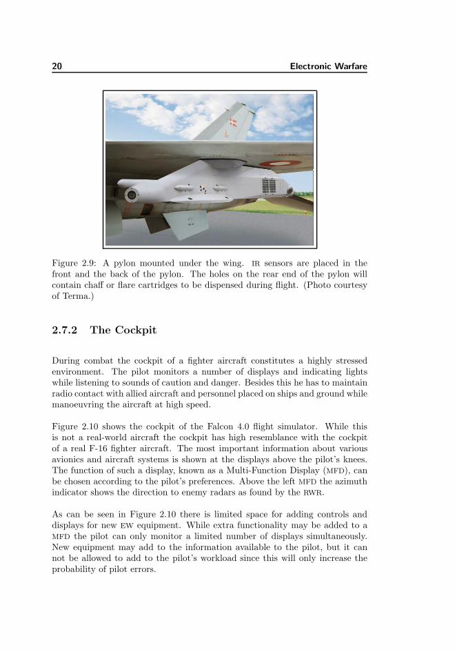
performance of the aircraft with only minor structural changes some of thestations may be equipped with pylons. A pylon may carry e.g. the IR sensorsfor a MWS, a jammer, a DIRCM unit, or cartridges of chaff or flares. While apylon takes up a station on the aircraft some pylons may function as stationsthemselves. Unfortunately pylons will often increase e.g. the RCS of the aircraft,and having them installed on the aircraft will thus not always improve thesurvivability of the aircraft.
20 Electronic Warfare
Figure 2.9: A pylon mounted under the wing. IR sensors are placed in thefront and the back of the pylon. The holes on the rear end of the pylon willcontain chaff or flare cartridges to be dispensed during flight. (Photo courtesyof Terma.)
2.7.2 The Cockpit
During combat the cockpit of a fighter aircraft constitutes a highly stressedenvironment. The pilot monitors a number of displays and indicating lightswhile listening to sounds of caution and danger. Besides this he has to maintainradio contact with allied aircraft and personnel placed on ships and ground whilemanoeuvring the aircraft at high speed.
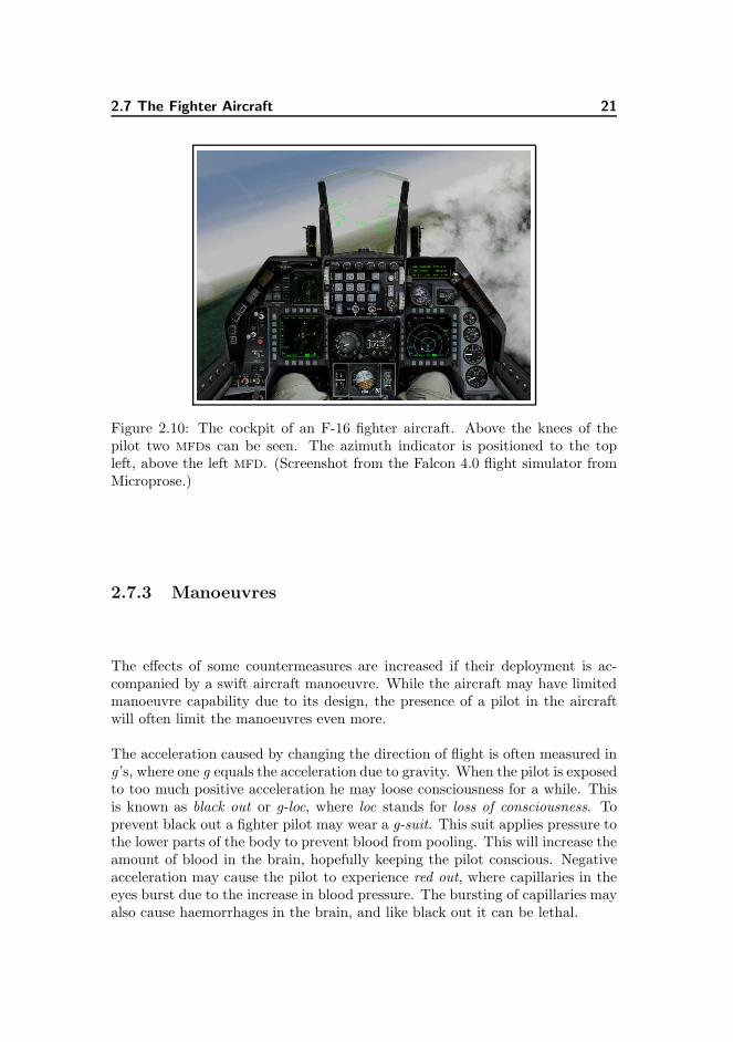
Figure 2.10 shows the cockpit of the Falcon 4.0 flight simulator. While thisis not a real-world aircraft the cockpit has high resemblance with the cockpitof a real F-16 fighter aircraft. The most important information about variousavionics and aircraft systems is shown at the displays above the pilot’s knees.The function of such a display, known as a Multi-Function Display (MFD), canbe chosen according to the pilot’s preferences. Above the left MFD the azimuthindicator shows the direction to enemy radars as found by the RWR.
As can be seen in Figure 2.10 there is limited space for adding controls anddisplays for new EW equipment. While extra functionality may be added to aMFD the pilot can only monitor a limited number of displays simultaneously.New equipment may add to the information available to the pilot, but it cannot be allowed to add to the pilot’s workload since this will only increase theprobability of pilot errors.
2.7 The Fighter Aircraft 21
Figure 2.10: The cockpit of an F-16 fighter aircraft. Above the knees of thepilot two MFDs can be seen. The azimuth indicator is positioned to the topleft, above the left MFD. (Screenshot from the Falcon 4.0 flight simulator fromMicroprose.)
2.7.3 Manoeuvres
The effects of some countermeasures are increased if their deployment is ac-companied by a swift aircraft manoeuvre. While the aircraft may have limitedmanoeuvre capability due to its design, the presence of a pilot in the aircraftwill often limit the manoeuvres even more.
The acceleration caused by changing the direction of flight is often measured ing’s, where one g equals the acceleration due to gravity. When the pilot is exposedto too much positive acceleration he may loose consciousness for a while. Thisis known as black out or g-loc, where loc stands for loss of consciousness. Toprevent black out a fighter pilot may wear a g-suit. This suit applies pressure tothe lower parts of the body to prevent blood from pooling. This will increase theamount of blood in the brain, hopefully keeping the pilot conscious. Negativeacceleration may cause the pilot to experience red out, where capillaries in theeyes burst due to the increase in blood pressure. The bursting of capillaries mayalso cause haemorrhages in the brain, and like black out it can be lethal.
22 Electronic Warfare
2.8 Summary
This chapter describes the domain of EW as the ”battle of the electromagneticspectrum”. Threats may detect a fighter aircraft using radiation within one ormore of the bands in the electromagnetic spectrum. Once the aircraft is detecteda missile may be launched against it. This missile is most likely guided towardsthe aircraft using electromagnetic radiation. If the guidance system is passiveit will rely on radiation emitted from the aircraft, e.g. IR radiation from hotparts of the airframe. A RF guided missile is an example of an active guidancesystem. It will emit radar radiation itself, and use the radiation echoed off theaircraft to determine the distance to, and possibly the velocity of, the aircraft.
The pilot may use ESM to gain knowledge about the current threat scenario.RWR and MWS are two such ESM systems. To counter threats the pilot may usedifferent forms of ECM. ECM can either be equipment on-board the aircraft or itcan be expendables dispensed into open air. When a missile is locked onto theaircraft the lock may be broken by appropriate use of ECM. The pilot may alsouse ECM preemptively to prevent threats from obtaining a lock on the aircraft.To reduce the effect of aircraft ECM the ground based threat may use EPM
technologies. Using these may reduce the probability of the aircraft recognizingthe threat or the threat being jammed by an aircraft jammer.
Chapter 3
Decision Support System in a
Fighter Aircraft
On modern fighter aircraft more and more systems are implemented in order toimprove the pilot’s awareness about the current situation of the aircraft and theworld surrounding it. As the number and complexity of these systems increaseso does the quantity of threats to the aircraft and appropriate countermeasuresfor the pilot to choose from. To help the pilot decide on a proper evasive actionwhen a threat occurs a Decision Support System (DSS) can be implementedaboard the aircraft [16, 20, 24].
This chapter describes the need for a DSS in a fighter aircraft, the requirementssuch a system must comply with, and the flow of data on which decisions fromthe system has to be made. Existing experimental and operational systems arealso described.
3.1 Problem Description
In [37] a DSS is described as ”a collection of computer-based interactive appli-cations, which based on domain specific knowledge and information supports adecision maker in one or more phases of the decision process.” A DSS may be
24 Decision Support System in a Fighter Aircraft
based upon an expert system which is a computer program that builds upondomain-specific knowledge from one or more experts. A DSS for fighter pilotswill build upon expert knowledge within the field of EW.
Missiles may be fired from ground or sea based launch pads, or they may be firedfrom enemy fighter aircraft in an air-to-air engagement. In the latter case theworkload on the pilot will be higher than it will be for land or sea based threatssince the position, altitude, and speed of the enemy aircraft must be taken intoconsideration as well. In this work the subject is to investigate means to designa DSS for finding responses to ground based threats only.
When engaged by ground based threats one or more missiles may be launchedtowards the aircraft. The pilot may choose to use countermeasures to avoidthe impact of an approaching missile. The countermeasures to choose dependon e.g. the type of missile, the distance and direction between the aircraft andthe missile, the hostility of the environment, altitude of the aircraft, and theavailability of countermeasures. Knowledge about threats that may be met inthe near future may also influence the choice of proper countermeasures andthe sequence in which they are used. If the aircraft is equipped with a limitedamount of expendable countermeasures it might reduce the survivability of theaircraft for the entire mission if at any given time more expendables were usedthan necessary, thus leaving none for a later necessity.
Prototypes for the DSS are designed using techniques from the fields of ArtificialIntelligence (AI) and Operations Research (OR). From the field of AI the pos-sibility of using the Prolog programming language is examined. This is chosensince the tactics for responses to ground based threats can be formulated as aset of rules that can be implemented using Prolog.
At DDRE a Master’s thesis has been written on the subject of using BayesianNetwork (BN) for decision support for fighter pilots [16]. BN may also be consid-ered as an AI technology, and it is chosen to expand on the experiences gainedby that work by examining further use of BN.
The decisions suggested to the fighter pilot may improve if the DSS is designedto handle temporal aspects. These aspects may describe limits on the use ofcountermeasures during a mission. For this it is chosen to describe the problemusing OR techniques. The problem is described by a mathematical model thatcan be solved to optimality. A metaheuristic is also applied, and here a trade-offbetween the quality of solutions and the time it takes to find them is made.
3.2 Survivability 25
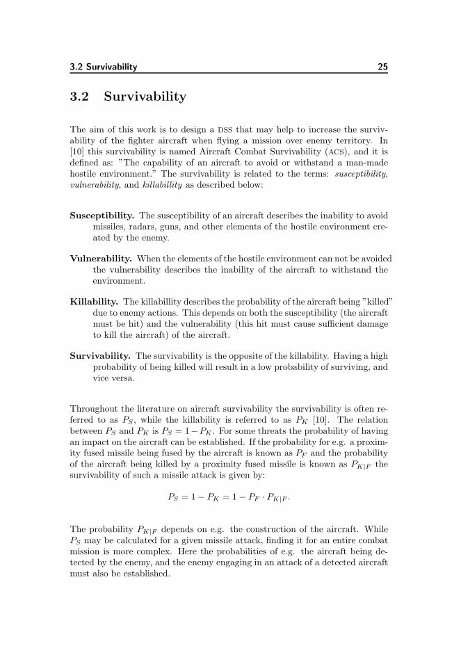
3.2 Survivability
The aim of this work is to design a DSS that may help to increase the surviv-ability of the fighter aircraft when flying a mission over enemy territory. In[10] this survivability is named Aircraft Combat Survivability (ACS), and it isdefined as: ”The capability of an aircraft to avoid or withstand a man-madehostile environment.” The survivability is related to the terms: susceptibility,vulnerability, and killabillity as described below:
Susceptibility. The susceptibility of an aircraft describes the inability to avoidmissiles, radars, guns, and other elements of the hostile environment cre-ated by the enemy.
Vulnerability. When the elements of the hostile environment can not be avoidedthe vulnerability describes the inability of the aircraft to withstand theenvironment.
Killability. The killabillity describes the probability of the aircraft being ”killed”due to enemy actions. This depends on both the susceptibility (the aircraftmust be hit) and the vulnerability (this hit must cause sufficient damageto kill the aircraft) of the aircraft.
Survivability. The survivability is the opposite of the killability. Having a highprobability of being killed will result in a low probability of surviving, andvice versa.
Throughout the literature on aircraft survivability the survivability is often re-ferred to as PS , while the killability is referred to as PK [10]. The relationbetween PS and PK is PS = 1−PK . For some threats the probability of havingan impact on the aircraft can be established. If the probability for e.g. a proxim-ity fused missile being fused by the aircraft is known as PF and the probabilityof the aircraft being killed by a proximity fused missile is known as PK|F thesurvivability of such a missile attack is given by:
PS = 1− PK = 1− PF · PK|F .
The probability PK|F depends on e.g. the construction of the aircraft. WhilePS may be calculated for a given missile attack, finding it for an entire combatmission is more complex. Here the probabilities of e.g. the aircraft being de-tected by the enemy, and the enemy engaging in an attack of a detected aircraftmust also be established.
26 Decision Support System in a Fighter Aircraft
3.3 Design Requirements
A DSS for fighter pilots must fulfil a number of requirements to be applicableduring a mission. Below six of these requirements are described. In designinga method for suggesting actions to the pilot these requirements must be takeninto consideration. In Chapter 8 the requirements are used in comparing fourapproaches for developing the DSS.
Real-time. The system has to find solutions to occurring threats in near real-time. It may take as little as 2-3 seconds from a missile has been launcheduntil it reaches the aircraft. Before actions can be taken to avoid theincoming missile, sensors on-board the aircraft must detect the missile,the system must find an appropriate set of actions, and these actionsneed to be presented to the pilot. To give the pilot adequate time toperform evasive actions it is estimated that the system has approximately200 milliseconds from a change in the threat scenario occurs until a set ofactions has to be suggested to the pilot.
Hardware. Since a final implementation of the system must be run in a fighteraircraft, the hardware required for developing the system must match therequirements given to hardware in the aircraft. The results from a DSS
depends on data input from other devices on-board the aircraft and henceit must be easy to integrate the DSS with these systems.
Updateable. The descriptions of threats and guidance systems are constantlyevolving as are new countermeasure systems. Therefore, the system de-veloped must be easily updated and maintained [24]. To ensure this thesystem must preferably be data driven, and updating the system will thenbe a matter of updating data on missile systems, guidance methods, etc.The algorithms used must have none or minor updates only.
Trustworthy. Any solution from the system must seem reasonable to the pi-lot. Otherwise the system will not be trusted and hence not used. Thisrequirement can be divided into two sub-requirements: the system mustsuggest a reasonably solution to any changes in the scenario, e.g. whena new threat occurs, and when no threats are imminent no suggestionsshould be given.
Both in combat and during tests in the development phase the user of thesystem will be a fighter pilot. If the pilot does not understand how thesolutions suggested by the system can be inferred he may not trust theirvalidity. Therefore the concept of the inferring parts of the system mustbe relatively easy to understand.
3.4 Mission Data Flow 27
Useful. The usefulness of a DSS is its ability to improve the survivability of thepilot. If the system is limited to only suggest actions to the pilot withina fraction of all the situations he may find himself and the aircraft in itis of no use. The difference between this requirement and the previous isthat a system may be trustworthy only within given limits without beinguseful to the pilot. An example hereof is a system that suggests actionsto mitigate e.g. RF threats only.
User Interface. Results from the system must be presented to the pilot insuch a way that they are easy and fast to interpret. The presentation canbe visual, use audio, or be a combination of both. During the evaluationof possible techniques for developing the system the presentation of thesuggested action is of minor importance. In the development of a systemthat is to be fielded this requirement must take a high priority.
In [24] more issues are mentioned as critical to the design of a DSS. Among theseissues are the use of data compression techniques, a user friendly database inter-face for updating the data used by the system, and effective memory manage-ment. None of these issues are considered crucial in this work and the handlingof these is beyond the scope of the work.
Data from different sensors, or from the same sensor over a period of time,may be fused to give the pilot a better situational awareness. The discipline ofperforming data fusion is a topic of its own, and it too is considered beyond thescope of the work.
3.4 Mission Data Flow
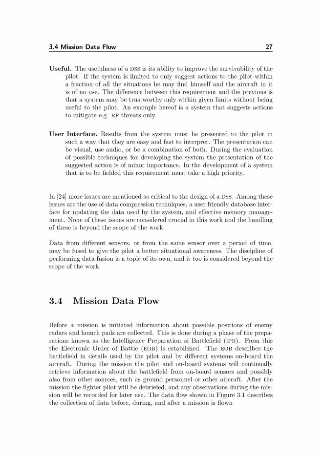
Before a mission is initiated information about possible positions of enemyradars and launch pads are collected. This is done during a phase of the prepa-rations known as the Intelligence Preparation of Battlefield (IPB). From thisthe Electronic Order of Battle (EOB) is established. The EOB describes thebattlefield in details used by the pilot and by different systems on-board theaircraft. During the mission the pilot and on-board systems will continuallyretrieve information about the battlefield from on-board sensors and possiblyalso from other sources, such as ground personnel or other aircraft. After themission the fighter pilot will be debriefed, and any observations during the mis-sion will be recorded for later use. The data flow shown in Figure 3.1 describesthe collection of data before, during, and after a mission is flown
28 Decision Support System in a Fighter Aircraft
Figure 3.1: Mission data flow.
3.4.1 Intelligence Preparation of Battlefield
The IPB is described as a military method for collecting and processing in-telligence about the battlefield [30]. The method describes how accurate andrelevant intelligence may be organized and provided to a military decision makerin a timely fashion.
Sources for intelligence may vary from eyewitness statements and reports frommilitary personnel to radio intercepts and satellite photos. The IPB describeshow intelligence is to be used to gain knowledge about the battlefield. It is arepeated process consisting of the four steps described below:
1. Define the battlefield. The battlefield is a geographical area and theairspace above it. The decision maker will concentrate on decisions re-garding forces within this area. The size of the area may vary duringcombat according to the knowledge of the battlefield available.
2. Describe the effects of the battlefield. Here the influence on the mission bye.g. the terrain or the current weather is established. This step may findcorridors in where the aircraft can fly without being detected by enemyradar, or routes in where the aircraft can remain almost invisible due tofog.
3. Evaluate the threat. A profile of the enemy’s capabilities within the bat-tlefield is created. This may e.g. include the number and positions ofenemy radar system.
4. Determine enemy courses of action. With the knowledge gained fromthe first three steps of the IPB the probable courses of enemy actions aredetermined.
3.5 System Data Flow 29
3.4.2 Electronic Order of Battle
The EOB is defined as a list of the locations, identifications, functions, andcapabilities of electronic equipment employed by a military force [41]. Thisinformation is made available to the pilot during the pre-flight preparation ofthe aircraft. Information about the planned route and current equipment andammunitions on the aircraft may also be loaded electronically to an aircraftcomputer. The planned route will often be described using a fixed number oflocations. Such a location is known as an Intermediate Point (IP).
The inventory consisting of countermeasures and weapons is based on the EOB.Since countermeasures and weapons will often have to share the same stationsplaced under the aircraft the more countermeasures that are deemed necessarythe fewer weapons may be carried. Generally the assessment of the battlefieldwill lie within one of the categories given below. While battlefields within someof these categories are estimated as being unlikely, they are mentioned here forcompleteness.
• The battlefield contains no known threats and the aircraft is not equippedwith ECM.
• The enemy has passive missiles only (e.g. MANPADS) and the aircraft willbe equipped with flares.
• The enemy has active missiles only and the aircraft will be equipped withchaff. This situation is unlikely.
• The enemy has active missiles only. These missiles may be jammed andthe aircraft is equipped with both chaff and jammer. This situation isunlikely as well.
• The enemy has multiple types of weapon or the composition of weaponsis unknown. The aircraft is equipped with chaff, flares, and a jammer.
• The enemy has passive missiles only or missiles that may be jammed. Theaircraft is equipped with jammer and flares. This situation too is unlikely.
3.5 System Data Flow
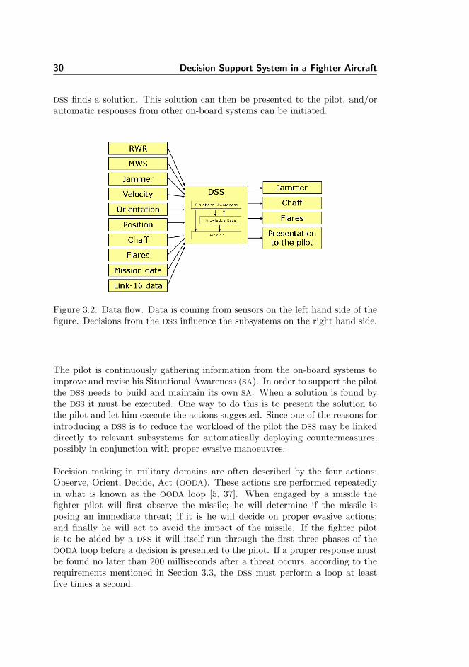
The basic data flow for the working environment of the DSS is shown in Figure3.2. At the left hand side data is fed to the DSS from different systems on-boardthe aircraft. With the aid of a knowledge base and the constructed SA the
30 Decision Support System in a Fighter Aircraft
DSS finds a solution. This solution can then be presented to the pilot, and/orautomatic responses from other on-board systems can be initiated.
Figure 3.2: Data flow. Data is coming from sensors on the left hand side of thefigure. Decisions from the DSS influence the subsystems on the right hand side.
The pilot is continuously gathering information from the on-board systems toimprove and revise his Situational Awareness (SA). In order to support the pilotthe DSS needs to build and maintain its own SA. When a solution is found bythe DSS it must be executed. One way to do this is to present the solution tothe pilot and let him execute the actions suggested. Since one of the reasons forintroducing a DSS is to reduce the workload of the pilot the DSS may be linkeddirectly to relevant subsystems for automatically deploying countermeasures,possibly in conjunction with proper evasive manoeuvres.
Decision making in military domains are often described by the four actions:Observe, Orient, Decide, Act (OODA). These actions are performed repeatedlyin what is known as the OODA loop [5, 37]. When engaged by a missile thefighter pilot will first observe the missile; he will determine if the missile isposing an immediate threat; if it is he will decide on proper evasive actions;and finally he will act to avoid the impact of the missile. If the fighter pilotis to be aided by a DSS it will itself run through the first three phases of theOODA loop before a decision is presented to the pilot. If a proper response mustbe found no later than 200 milliseconds after a threat occurs, according to therequirements mentioned in Section 3.3, the DSS must perform a loop at leastfive times a second.
3.5 System Data Flow 31
3.5.1 Acquiring Data
In order to decide on actions to suggest to the pilot the system needs input fromvarious sources. In most fighter aircraft these sources will be systems connectedto a data bus on-board the aircraft. In many aircraft this bus will comply withthe MIL-STD-1553B standard [4].
On a MIL-STD-1553B bus the communication is controlled by a bus controller.Data can come from a number of remote terminals, and it can be read by anumber of bus monitors. The bus controller serves as an arbiter that allows theremote terminals to use the bus one at a time. Data on the bus is transmitted asdatagrams from one remote terminal to one or more bus monitors. The formatof a datagram is described in an Interface Control Document (ICD), and sinceevery remote terminal may use a specific format for every bus monitor receivingdata from the terminal, a large number of ICDs may be needed to describecommunication on the bus. Since a DSS may need input from many remoteterminals, and these may vary from one aircraft to another, the DSS must bedesigned so it can be easily adapted to a comply with new sets of ICDs.
Most datagrams are transmitted with a relatively low frequency. If allowedby the bus controller a typical datagram will have a transmission frequency inthe order of 1 to 20 per second, depending on the assessed importance of thedatagram. Combined with a relatively low clock frequency controlling the bus,a slack time in the magnitude of 0.1 to 0.5 seconds may well appear betweenthe time a sensor system has detected a threat till a bus monitor (e.g. the DSS)receives notification about it. This slack leaves only a short period of time forthe DSS to find and suggest an action to the pilot.
Besides on-board sensor systems data to the DSS may be supplied through atactical data link. Link-16 is a standard for such a tactical data link, and it isused for sharing information (e.g. identification and voice commands) betweenallied units (aircraft, ships, etc.) in the battlefield. A DSS may benefit fromdata given through Link-16 to maintain a model of threats, their tracks, sizes,numbers, and positions.
The sensors and sources for detecting threats on-board the aircraft differ in sev-eral aspects. They operate in different bands of the electromagnetic spectrum,use different methods to determine the threats, and since they may interprettheir analogue input differently, they may not agree on the threats found. Togive the DSS a single ”ground truth” to work with, it may be essential that datafrom the different kind of sources are fused before handed to the system.
32 Decision Support System in a Fighter Aircraft
3.5.2 Threat Evaluation
Not all changes to the threat scenario will require the DSS to suggest new actions.Throughout a mission one of the goals of the DSS is to minimize the workloadof the pilot. Therefore, when the aircraft flies over friendly territory, and nothreats are imminent, no actions must be suggested by the DSS. As soon asthe MWS issues a warning, or the RWR detects radiation from a possibly hostileradar, the territory can no longer be considered friendly, and the system willsuggest actions to the pilot.
Even while flying over enemy territory the DSS must only suggest evasive actionswhen necessary. To determine when e.g. warnings from the RWR stem frompreviously undetected radar system, or if the radar has just reappeared on theRWR after being lost for a moment, a threat evaluator subsystem may be addedto the DSS. Such a subsystem will have to base its evaluation on a registrationof recent warnings. The RWR may loose track of radar systems if the aircraft ispositioned such that either itself or the terrain underneath it prevents the radarfrom being detectable by the RWR antennas. For the MWS some warnings canbe ignored too. If a warning is issued for a fraction of a second only, it is likelyto be caused by e.g. a reflection that is visible only for a moment, instead ofby a missile following the aircraft. If the threat evaluator has to compare everywarning to previous warnings, the first warnings of a threat will be ignored.When warnings are no longer ignored even less time is left for the DSS to find asolution.
3.5.3 Executing Decisions
In general a DSS will support a decision maker in deciding proper actions. Whenthe suggestions from a fighter aircraft DSS is presented to the pilot, the pilotwill have to decide on the actions to perform before carrying them out. Since alimited time is available for the pilot to do this the DSS can perform the actionsitself; even without the consent of the pilot. Most fighter aircraft use fly-by-wirecontrol, i.e. all controls are entirely electronic. This means that the DSS cantake control of the aircraft and perform the proper manoeuvres while dispensingexpendables. While this may be technical feasible it is not necessarily a situationwanted by the pilot. According to [39] nine of ten interviewed pilots said thathaving the aircraft taking control was anathema to them.
Having the DSS working in interaction with some of the ECM system on-board theaircraft, without taking complete control, may still improve the survivability ofthe aircraft. The DSS may e.g. notify the jammer about RF threats not detected
3.6 Models and Systems 33
by the jammer itself, or it may release flares or chaff when the aircraft is flyingin the proper direction. While the control of the aircraft remains in the handsof the pilot, the DSS will increase his survivability and part of his workload willbe taken from him.
3.6 Models and Systems
The approaches to the development of a fighter aircraft DSS described in thiswork are not the first attempts on introducing a DSS into the field of aviation.This section describes a number of experimental models that may be used in aDSS, and a few existing systems. Some of the models use techniques from thefields of AI and OR, such as fuzzy sets, mimic nets, and genetic programming.These techniques are not described here.
3.6.1 Experimental Models
The Countermeasure Association Technique (CMAT) automatically recommendscountermeasures and manoeuvres to a pilot under missile attack [24]. The tech-nique selects responses that will increase the survivability in relation to both thecurrent and future threats. It is done by fusing possibly incomplete sensor inputand feeding the results to a mimic net. A set of combat scenarios is presentedto EW experts and the mimic net is trained to mimic the responses from theseexperts. Solutions found by the CMAT are called strategies, and given a threatscenario, a number of strategies are found. The best of these strategies, i.e. thestrategy that best mimics the responses from EW experts, is chosen.
In 1986 the Pilot’s Associate project was initiated by the United States De-fense Advanced Research Projects Agency [11, 39, 48, 49]. The concept of thePilot’s Associate is a set of knowledge-based subsystems: two assessors, twoplanning subsystem, and a Pilot-Vehicle Interface (PVI). The Situation Assess-ment subsystem determines the current state of the outside world, while theSystem Status subsystem acquires knowledge about the state of on-board sys-tems. The Tactics Planner subsystem supports the pilot in choosing responsesfrom possible alternatives when immediate threats occur. In case of deviationsfrom the mission plan the Mission Planner will adapt the plan to the currentsituation. The PVI adapts the information shown to the pilot to the currentsituation. When for instance the pilot needs to respond to an imminent threat,warnings that can be delayed, e.g. of malfunctioning subsystems, will not beshown.
34 Decision Support System in a Fighter Aircraft
In [48, 49] the Pilot’s Associate is compared to a French system named CopiloteElectronique. This system is based on an in-depth analysis of the pilot’s cognitiveprocessing, and the aim is to find ways to support the pilot based on his currentactivities and an estimation of his current mental workload.
The concept of General Aviation Pilot Advisory and Training System (GAPATS)is to run a flight management system on an inexpensive PC [33]. It is inspired bythe Pilot’s Associate system, and it consists of two main parts, the Flight ModeInterpreter (FMI), and the Pilot Advisor (PA). Based on e.g. aircraft statevariables, such as altitude, airspeed, and rate of climb, the FMI determines thecurrent flight mode (taxi, take off, cruise, etc.). This is done using fuzzy setsand the result is continually fed to the PA. Based on the current flight mode anda set of rules the PA will use the Heads-Up Display (HUD) and the Heads-DownDisplay (HDD) to display relevant information to the pilot.
The Missile Countermeasure Optimization (MCO) problem is the subject of anumber of papers, e.g. [31, 32]. In [31] the aim is to combine aircraft manoeuvresand countermeasures to survive an attack from a single surface-launched anti-aircraft missile. The best combination of countermeasures and manoeuvres isfound using genetic programming. The method encompasses uncertainties aboutboth the type and the state of the approaching missile.
The Automated Threat Response using Intelligent Agents (ATRIA) system isdescribed in [36]. Here Prolog is used in implementing asset agents. An assetagent represents a military asset such as a missile and/or aircraft tracking sys-tem, a radar system, or a missile. The agents in the system share an evolvingdescription of the combat scenario, and while finding responses for themselvesthey communicate these to other friendly assets in the battlefield.
In [47] the use of temporal reasoning in the process of decision-making is de-scribed. Here the scenario is Beyond Visual Range (BVR) combat with multipleenemy aircraft, and the scope is to give the pilot a visual interpretation of thesituation. For each of the enemy aircraft a goodness value is calculated, indi-cating which aircraft will have the upside in a close encounter. The goodnessvalue is based on the time it will take for each aircraft to initiate appropriateactions. BNs are suggested as a means of evaluating the properties of an enemyfighter aircraft.
In [19] chaff and flare programs are optimised using a statistical model. Thismodel express the survivability as a function of various parameters includingmissile attack rate, false alarm rate, missile detection probability, and the du-ration of a mission. The goal of the work described is not to optimise thesurvivability in a specific scenario, but rather to study how different parametersaffect the chaff and flare programs.
3.6 Models and Systems 35
3.6.2 Existing Systems
An Integrated Defensive Aids System (IDAS) is a system that collects inputfrom different sources, and combines these to e.g. automatically dispense ex-pendables or utilize a jammer to counter enemy systems. Input may come fromdifferent sensors on-board the aircraft, or it may be relayed from sensors onother platforms such as other aircraft, or ground- or sea-based sensor systems.Historically EW equipment on an aircraft has been considered as add-on unitsand not as integrated parts of the aircraft. In [52] it is mentioned that an IDAS
must be considered as an integrated part of the aircraft systems in much thesame way as the engine, and it is argued that the role of both is to get the air-craft to the target and back. Each of the two systems described in this sectioncan be regarded as an IDAS.
The Electronic Warfare Management System (EWMS) is developed by Termato reduces the pilot’s workload and to ensure coordinated and effective useof on-board EW systems [51]. It can be operated in three modes: In manualmode the pilot activates the countermeasure program to use. When in semi-automatic mode the Electronic Combat Adaptive Processor (ECAP) will analyzethe presence of threats and chose an effective combination of countermeasures.This combination is presented to the pilot who can give his consent by activatinga switch. After consent is given a script for the combination of countermeasuresis initiated. The pilot does not need to give his consent when the system is inautomatic mode. A script related to the best use of countermeasures found willbe initiated.
The Threat Response Processor (TRP) is developed at Georgia Tech ResearchInstitute (GTRI) [55]. It is a combination of straightforward improvements ofthe survivability and an expert system, and it has undergone extensive flighttesting over more than seven years. At first inputs from various systems on-board the aircraft are correlated, ambiguities are handled, and inputs describinge.g. different threats are prioritized. After this a number of scripts are spawned,depending on the character of the input. Among other things these scripts selectproper countermeasures to apply and messages to display to the pilot. Aftereach spawned script is executed the optimal response is found from the resultsof the scripts. This response is then fed to the EWMS to handle e.g. dispensingof expendables.

36 Decision Support System in a Fighter Aircraft
3.7 Summary
This chapter describes the need for a fighter aircraft DSS to assist the pilot infinding the best responses when being engaged by ground-based threats. Sincesolutions from a DSS are intended to improve the survivability of the pilot,the concept of survivability is introduced. The survivability depends on thesusceptibility, vulnerability, and killabillity of the aircraft.
A DSS must comply with a number of design requirements. Requirements toresponse time, ability to run on aircraft hardware, ability to be easily updated,and the system being both trustworthy and useful are described. In addition tothis a DSS must have an easy to use user interface/PVI. The design of the userinterface is outside the scope of the work.
A DSS will work on mission data in determining optimal responses. The missiondata flow is described, and the concepts of Intelligence Preparation of Battlefield(IPB) and Electronic Order of Battle (EOB) are introduced. When airborne theDSS relies on data from on-board sources. Data may often be acquired via anaircraft data bus. MIL-STD-1553B is a standard for such a bus, and some ofthe characteristics of this standard are mentioned.
Experimental models and existing systems are described. The experimentalmodels apply techniques from the fields of AI and OR while systems that hasalready been implemented in aircraft seem to use more pragmatic approaches.
Chapter 4
The Prolog Approach
Prolog is a programming language for describing relations using logic. The nameProlog is the short concatenation of PROgramming and LOGic. In constructinga DSS Prolog can be applied for the formulation of a set of rules for the responsesto ground-based threats and launched missiles. This chapter describes how touse the Prolog programming language for analysing a threat scenario, and forthe construction of a Prolog based DSS.
Starting with some logic theory the basics of Prolog theory is introduced. Sometextbooks on AI describe the terminology used in logic, and the use of logic ininferencing. See [54] for more details on logic, and [12, 56] for introductions toProlog. The introductions of logic and Prolog in this chapter aim at providingthe background for understanding the Prolog based DSS developed. This DSS isintroduced in Section 4.5.
4.1 Motivation
When a fighter pilot is taught the essentials about reacting to ground-basedthreats, he is essentially given a set of rules to follow. These rules can beformulated in natural language by experts in the domain of EW. Rules such as
38 The Prolog Approach
”if you get a missile warning, and not a radar warning, a missile using infraredguidance is launched” or ”if you keep the altitude low enough, you can escaperadar based threats” can be reformulated in Prolog, and used in the foundationof a Prolog-based DSS.
The set of rules written in Prolog is referred to as a Prolog program, and to useit for decision support, it should be fed to a computer program for execution. Inthis work the program executing the Prolog program is referred to as the Prologinterpreter, although Prolog programs can also be executed as compiled code.Since Prolog interpreters exist on many computer platforms, and input such assensor responses and mission descriptions can easily be given using Prolog, thedevelopment of a Prolog based DSS does not require any special system setup.
Although many Prolog interpreters have features that enhance the strength ofProlog, ”pure” Prolog is a relatively simple programming language. Thereforeimplementing a Prolog interpreter on a computer platform usable in a fighteraircraft is a feasible task, and transferring a desktop version of a DSS to anaircraft can be expected to be smoothly done.
It is estimated that writing a program in Prolog will often require far less de-velopment time than writing an equivalent program in e.g. C or C++ [12]. Thesyntax of Prolog programs makes them relatively easy to read, even for peoplewith little or no programming experience. This helps in the validation of a DSS,since this can then be done partly by domain experts. If care is taken duringdevelopment, and the program is written in an almost self-explanatory way, thetask of maintaining a Prolog based DSS can relatively easy be done by peopleother than the original developers.
Even if Prolog may not be the preferred technique to use for a DSS, a Prologbased program may be used to test a DSS based on other techniques. If theanswers from the Prolog system have been validated, it can be used as a look-up table for the ”correct” responses in the scenarios it is used to evaluate.
4.2 Basic Theory
This section presents some basic theory about logic and Prolog. The vocabu-laries on both logic and Prolog are relatively large, and some of the basic termsare introduced here.
In essence the interactions in a domain, and data describing it, are given inProlog using a set of rules. These rules are described in one or more files, which
4.2 Basic Theory 39
can be interpreted by a Prolog interpreter. When doing so, the interpreter cananswer questions about the domain, in accordance to the rules given. Prologassumes a closed world, meaning that anything not explicitly declared is perdefinition non-existing.
Some Prolog systems offer graphical user interfaces, database connectivity, spe-cial constructs for software-based agents, and other features that enhance theusability of the system. For the evaluation of Prolog as the base of a DSS, suchconstructs are not necessary and they will not be described here.
Programming languages such as C/C++ are classified as imperative, whichmeans that programs written using these languages describes the steps nec-essary for a program to evaluate input and produce output. These steps aredescribed using statements, and the order of execution of these statements isdetermined by the programmer. As opposed to the imperative languages, Pro-log is a declarative programming language. Here the emphasis is on declaringthe relations between input and output, and not on how these relations shouldbe implemented by the programmer.
4.2.1 Logic
Logic is a mathematical discipline working with statements that can be eithertrue or false. This is done using predicates, which are functions mapping theirarguments into true/false. A predicate with arguments, or a negation of thepredicate, is known as a literal. When using logic in describing a domain,the description may include objects. Variables ranging over the objects of thedomain can also be included.
Treating weather as an object, it can be described using a number of vari-ables such as precipitation in millimetres, temperature in centigrade, etc. Somequestions about the weather, such as ”is it raining?” or ”is it cloudy?” can beanswered using the logical values true and false, while others may need an in-terpretation of the aforementioned variables. The question ”Is it warm?” couldrelate to the temperature: ”If the temperature is above 15◦C, it is warm”. Thiswould map the temperature in to true/false.
As literals can take the values true and false, so can combinations of literals.Four of the basic combinations, known as logical connectives, are or (∨), and(∧), not (¬), and implies (⇒).
When literals are joined using the and -connective, they form a conjunction,where each part is known as a conjunct. Similarly, when joined using or, they
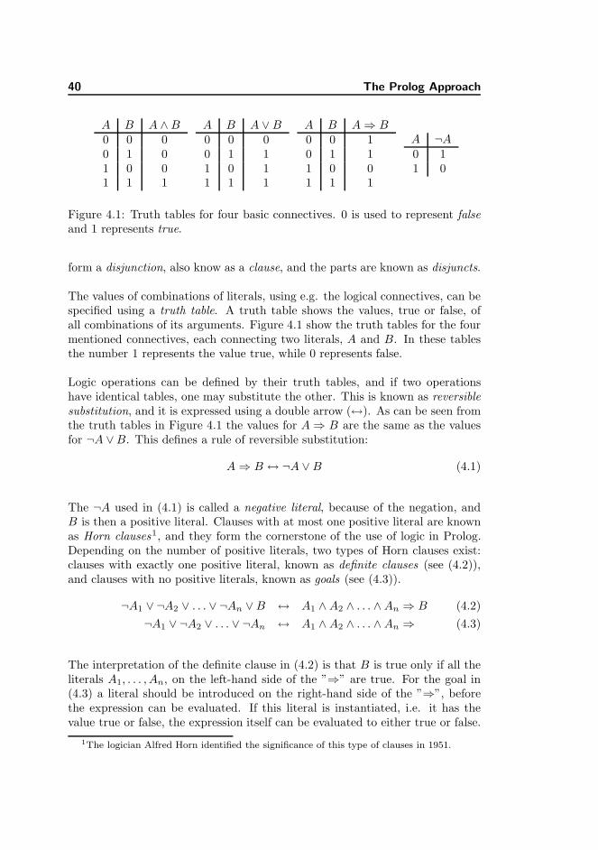
40 The Prolog Approach
A B A ∧B0 0 00 1 01 0 01 1 1
A B A ∨B0 0 00 1 11 0 11 1 1
A B A⇒ B0 0 10 1 11 0 01 1 1
A ¬A0 11 0
Figure 4.1: Truth tables for four basic connectives. 0 is used to represent falseand 1 represents true.
form a disjunction, also know as a clause, and the parts are known as disjuncts.
The values of combinations of literals, using e.g. the logical connectives, can bespecified using a truth table. A truth table shows the values, true or false, ofall combinations of its arguments. Figure 4.1 show the truth tables for the fourmentioned connectives, each connecting two literals, A and B. In these tablesthe number 1 represents the value true, while 0 represents false.
Logic operations can be defined by their truth tables, and if two operationshave identical tables, one may substitute the other. This is known as reversiblesubstitution, and it is expressed using a double arrow (↔). As can be seen fromthe truth tables in Figure 4.1 the values for A⇒ B are the same as the valuesfor ¬A ∨B. This defines a rule of reversible substitution:
A⇒ B ↔ ¬A ∨B (4.1)
The ¬A used in (4.1) is called a negative literal, because of the negation, andB is then a positive literal. Clauses with at most one positive literal are knownas Horn clauses1, and they form the cornerstone of the use of logic in Prolog.Depending on the number of positive literals, two types of Horn clauses exist:clauses with exactly one positive literal, known as definite clauses (see (4.2)),and clauses with no positive literals, known as goals (see (4.3)).
¬A1 ∨ ¬A2 ∨ . . . ∨ ¬An ∨B ↔ A1 ∧A2 ∧ . . . ∧An ⇒ B (4.2)
¬A1 ∨ ¬A2 ∨ . . . ∨ ¬An ↔ A1 ∧A2 ∧ . . . ∧An ⇒ (4.3)
The interpretation of the definite clause in (4.2) is that B is true only if all theliterals A1, . . . , An, on the left-hand side of the ”⇒” are true. For the goal in(4.3) a literal should be introduced on the right-hand side of the ”⇒”, beforethe expression can be evaluated. If this literal is instantiated, i.e. it has thevalue true or false, the expression itself can be evaluated to either true or false.
1The logician Alfred Horn identified the significance of this type of clauses in 1951.
4.2 Basic Theory 41
If the literal is an un-instantiated variable, it should retrieve the value (true orfalse), which will make the evaluation of the expression return true.
Consider the special case of (4.3) with n = 2: A1∧A2 ⇒. Having A1 = true andA2 = false, and introducing the literal B on the right-hand side, the expressionbecomes: true ∧ false ⇒ B. If B itself evaluates to true, the goal is false(true ∧ false ; true), while the goal is true if the value of B is false. If B isa variable it should therefore receive the value false, since this would make thegoal evaluate to true.
4.2.2 Horn Clause Logic
Horn clauses are often written with the positive literal to the left, the directionof the implication arrow reversed, and using commas for or, instead of ∧:
B ⇐ A1, A2, . . . , An (4.4)
The literals on the right-hand side of the ’⇐’ constitute the premises (an-tecedents), and the literal on the left-hand side is the conclusion (consequent).
In Prolog the names clauses, predicates, rules, and functions are all synonymouswith Horn clauses. Here the arrow is substituted by a colon and a dash:
b :- a1, a2, ..., an (4.5)
The clause in (4.5) can be read as ”b is true, if all the values on the right-handside are true”. In Prolog literals starting with a capital letter are interpreted asvariables (described later), and the literals used in (4.5) are thus written usingminuscule letters.
If a literal serve as the consequent in multiple clauses in a Prolog program, theantecedents may be concatenated using a semi-colon:
b :- a1, a2; c1, c2 (4.6)
The clause in (4.6) can be read ”b is true if a1 and a2 are both true, or if c1 andc2 are both true”. The semi-colon can be interpreted as an or connective, andit has a higher precedence than and. Parentheses can be introduced to alter thebindings of the colons and semi-colons.
42 The Prolog Approach
The clauses may be divided into facts, relations, and directives. Common to allof these is that they must be terminated by a full stop. For the readability ofthis text, the full stop is often omitted.
The building blocks of Prolog are atoms and variables. An atom is a concretevalue, which can be a name (manpads), a string (’Turn left’) or a numericalvalue (600). All names have a minuscule as the first character.
Variables are used in enquiring about the contents of the facts given (see Section4.2.2.1). As opposed to atoms variables are always written with a capital as thefirst character. Variables starting with the underscore (’ ’) is an exception ofthis. These are known as anonymous variables, since their names can not bereferenced. See Section 4.3.2 for an example of questioning with Prolog usingatoms and variables.
4.2.2.1 Facts
A fact is a clause with no antecedent, and it is unconditionally true. Factsmay be unary, and if so, they are statements about their single argument, suchas ac type(fighter) or altitude(600). The interpretation of a fact is deter-mined by the programmer, and these two facts may state that the DSS is used ina fighter aircraft flying at an altitude of 600 m. Here ac type and altitude arethe names of the facts, while fighter and 600 are arguments to them. Whenmore facts share the same name, each of these are said to be an instance of thefact.
If a fact has two or more arguments, it describes a relation between these ar-guments. An example of such a fact is guidance(manpads, ir), declaringthat MANPADS are using IR guidance. Prolog has no requirements to the or-der of arguments in a relation, and it is up to the programmer to keep theorder of the arguments in similar facts. If the first argument in the guidance
fact is defined to be a threat, and the second is a guidance system, then theguidance(manpads, ir) is a valid fact, with respect to this definition. SinceCommand is a guidance system and SA-2 is a threat the guidance(command,
sa2) fact is not valid. Prolog has no understanding of guidance and it will notknow valid facts from invalid facts. If it is asked about e.g. the guidance systemswith these two facts, it would give ir and sa2 as answers.
4.2 Basic Theory 43
4.2.2.2 Predicates
A predicate has the antecedents-consequent structure as seen in (4.5) and (4.6).Whereas a fact is unconditionally true, a consequent in a predicate is only trueif the antecedents are true. The antecedents can be either facts or predicates,or they can be comparisons of results from arithmetic operations.
The example below illustrates the use of both facts and predicates in describingthe weather:
% Facts about the weather
precipitation(rain).
weather(cloudy).
temperature(21).
% Predicates, describing the weather
it_is_warm :-
temperature(T),
T > 15.
weather_is_good :-
it_is_warm,
weather(sunny),
not(precipitation(_)).
The predicate it is warm will evaluate to true, since a fact is stating thatthe temperature is above 15◦C. Since it is raining and not sunny, the predicateweather is good will return false. The % mark a comment, and anything placedto the right of this is not interpreted by the Prolog interpreter. not is a standardProlog-procedure, which is described later.
4.2.2.3 Lists and Structures
In Prolog a list is a data structure containing a number of elements. The list isdescribed within square brackets; the empty list is denoted [], and non-emptylists have a head element and a tail, where the tail itself is a, possibly empty, list.The head has one or more elements, and it is separated from the tail by usingthe vertical bar: ([Head|Tail]). To reference e.g. the third element in a list,which is also the third element in the head of the list, one writes [ , ,Third| ],and the element is referenced by the variable named Third. Elements in a listmay be atoms, variables, lists, or structures.
44 The Prolog Approach
A structure is a collection of attributes used to describe objects. If a struc-ture is used to describe a person, the attributes may be the person’s name,age, and gender. Describing Tom, who is a 33 year old male, can then bedone by person(tom, 33, male). A family consisting of a mother, a fa-ther, and a number of children can be described as a structure of personsfamily(person( , ,female), person( , ,male), [ | ]). Here the list at theend ([ | ]) describes the children, and since this description has at least onehead element, the family has one or more children.
Structures can be used in goals, just like atoms or variables. In the exampleabove, the goal of finding families, where the father’s name is Tom, can beformulated as family(person(tom, , ), , ), and finding families with exactlytwo children is done by: family( , ,[ , ]). As can be seen from these exam-ples, working with structures often deal with the structures of data, rather thanthe contents of these structures.
4.2.2.4 Directives
Directives are used to make the Prolog interpreter perform various standardoperations, such as input/output, generating lists, etc. The number of direc-tives available varies from one Prolog implementation to another. Some of thestandard directives, used in the Prolog program described in 4.5, are explainedhere
The :-include(<filename>) directive is used to include the contents of otherProlog files into an embedding file. When this is met by the interpreter, thecontent of the file, given as argument, is read and interpreted, as was it part ofthe embedding file.
findall, bagof, and setof are procedures that will collect instances, fulfillingcertain criteria, into a single list. findall and bagof are equivalent, and willboth collect all instances into the list, thus allowing for multiple instances ofelements in the list. The setof procedure will produce a set of the instances,where each element of the set is only present once.
To output text to the screen the write procedure is used. If the argument to theprocedure is an atom (e.g. a string) it is written as it is, and if it is a variable,the value of this is written. To put a line break in the output the nl directiveis used.
The not predicate will return the negated value of its argument. If the argumentis a goal that can be fulfilled, using the not procedure will return no.
4.3 Answering Questions with Prolog 45
4.3 Answering Questions with Prolog
Prolog is used to perform two different, but related, tasks: describing a domain,and enquiring about it. In its simplest form the first task is done by writingthe Prolog program in one or more files, which can then be read by a Prologinterpreter, while the second task may be managed using a Prolog interpreterprompt.
This section describes how one may retrieve information using Prolog, and whata Prolog interpreter does to provide the information.
4.3.1 Matching
A question to the Prolog interpreter, also known as a goal, takes on the form ofa predicate, or a combination of predicates, and it may contain both atoms andvariables. The Prolog interpreter will try to make a match between the goaland the predicates given in the Prolog program.
A goal and a predicate match if they are either identical of if variables withinthem can be instantiated so they become identical. If this can be made theinterpreter either returns yes or the necessary values of any variables used inthe goal that will result in a match. If no match can be found, the interpreterreturns no.
Consider a Prolog program consisting of these three facts only:
precipitation(rain).
weather(cloudy).
temperature(21).
If the goal precipation(rain) is given to the interpreter, it will return yes,since a match can be made between the goal and the first fact in the program.Asking precipation(P) will have the interpreter return P = rain, since in-stantiating the variable P with the value rain will make the match. The goalwind(breeze) will not match any of the facts in the program and the answer isno. The same answer is returned if the goal is set to weather(sunny), althougha predicate named weather is part of the program.
Multiple goals can be given at the prompt. The goals are separated by a comma,if all goals should be fulfilled, or a semi-colon if matching one of the goals is

46 The Prolog Approach
sufficient.
The Prolog program above, describing the weather, can e.g. be used to deter-mine whether one wants to ride the bike to work. Suppose the precipitationcan be described using the atoms snow, rain, sleet, and fog. Now the goalprecipitation(snow); precipitation(rain); precipitation(sleet)wouldget the answer yes if either of the sub-goals can be matched. If only thecombination of sleet and snow would make the bike stay at home, the goalprecipitation(snow), precipitation(sleet) should be used.
4.3.2 Working with Prolog
Several Prolog interpreters exist for working with Prolog on a standard PC. Theone used in this work is B-Prolog, which offers a prompt interface for askingquestion about the Prolog program. For more information about B-Prolog seeAppendix E.
When working with B-Prolog the clauses are given in a number of files, whichare consulted by the Prolog interpreter, before it can provide information abouttheir contents. Suppose a file describes the guidance relation using the followingclauses:
guidance(sa2, command).
guidance(sa3, command).
guidance(stinger, ir).
guidance(stinger, uv).
At the Prolog prompt the goal guidance(Threat, Guidance) is given. In nat-ural language this should be interpreted as the question: ”which threats areusing which guidance system?” The interpreter then produces the answer:
Threat = sa2
Guidance = command ?
The question contains two variables, Threat and Guidance, and the answergiven is the first match found. The question mark at the end of the answer isthe Prolog prompt. To get further matches, a semi-colon can be entered at thisprompt, and the interpreter then provides the next match:
Threat = sa3
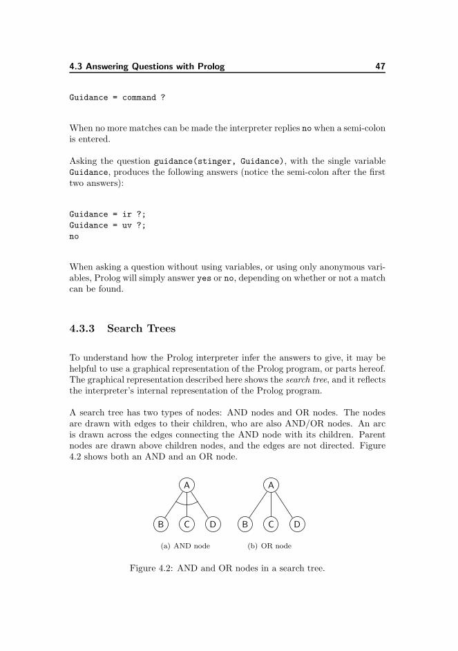
4.3 Answering Questions with Prolog 47
Guidance = command ?
When no more matches can be made the interpreter replies no when a semi-colonis entered.
Asking the question guidance(stinger, Guidance), with the single variableGuidance, produces the following answers (notice the semi-colon after the firsttwo answers):
Guidance = ir ?;
Guidance = uv ?;
no
When asking a question without using variables, or using only anonymous vari-ables, Prolog will simply answer yes or no, depending on whether or not a matchcan be found.
4.3.3 Search Trees
To understand how the Prolog interpreter infer the answers to give, it may behelpful to use a graphical representation of the Prolog program, or parts hereof.The graphical representation described here shows the search tree, and it reflectsthe interpreter’s internal representation of the Prolog program.
A search tree has two types of nodes: AND nodes and OR nodes. The nodesare drawn with edges to their children, who are also AND/OR nodes. An arcis drawn across the edges connecting the AND node with its children. Parentnodes are drawn above children nodes, and the edges are not directed. Figure4.2 shows both an AND and an OR node.
A
B C D
(a) AND node
A
B C D
(b) OR node
Figure 4.2: AND and OR nodes in a search tree.
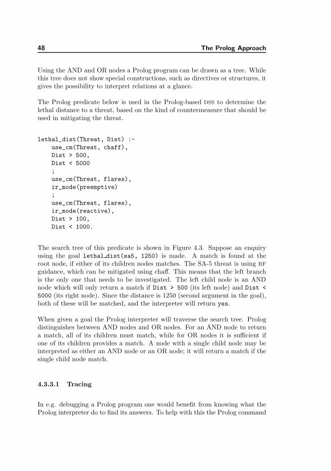
48 The Prolog Approach
Using the AND and OR nodes a Prolog program can be drawn as a tree. Whilethis tree does not show special constructions, such as directives or structures, itgives the possibility to interpret relations at a glance.
The Prolog predicate below is used in the Prolog-based DSS to determine thelethal distance to a threat, based on the kind of countermeasure that should beused in mitigating the threat.
lethal_dist(Threat, Dist) :-
use_cm(Threat, chaff),
Dist > 500,
Dist < 5000
;
use_cm(Threat, flares),
ir_mode(preemptive)
;
use_cm(Threat, flares),
ir_mode(reactive),
Dist > 100,
Dist < 1000.
The search tree of this predicate is shown in Figure 4.3. Suppose an enquiryusing the goal lethal dist(sa5, 1250) is made. A match is found at theroot node, if either of its children nodes matches. The SA-5 threat is using RF
guidance, which can be mitigated using chaff. This means that the left branchis the only one that needs to be investigated. The left child node is an ANDnode which will only return a match if Dist > 500 (its left node) and Dist <
5000 (its right node). Since the distance is 1250 (second argument in the goal),both of these will be matched, and the interpreter will return yes.
When given a goal the Prolog interpreter will traverse the search tree. Prologdistinguishes between AND nodes and OR nodes. For an AND node to returna match, all of its children must match, while for OR nodes it is sufficient ifone of its children provides a match. A node with a single child node may beinterpreted as either an AND node or an OR node; it will return a match if thesingle child node match.
4.3.3.1 Tracing
In e.g. debugging a Prolog program one would benefit from knowing what theProlog interpreter do to find its answers. To help with this the Prolog command
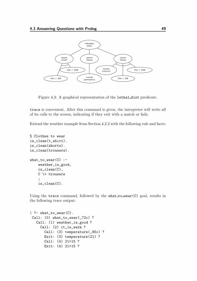
4.3 Answering Questions with Prolog 49
lethal dist(Dist)
use cm(chaff)
use cm(flares)
use cm(flares)
Dist > 500
Dist < 5000
ir mode(preemptive)
ir mode(reactive)
Dist > 500
Dist < 5000
Figure 4.3: A graphical representation of the lethal dist predicate.
trace is convenient. After this command is given, the interpreter will write allof its calls to the screen, indicating if they exit with a match or fails.
Extend the weather example from Section 4.2.2 with the following rule and facts:
% Clothes to wear
is_clean(t_shirt).
is_clean(shorts).
is_clean(trousers).
what_to_wear(C) :-
weather_is_good,
is_clean(C),
C \= trousers
;
is_clean(C).
Using the trace command, followed by the what to wear(C) goal, results inthe following trace output:
| ?- what_to_wear(C).
Call: (0) what_to_wear(_72c) ?
Call: (1) weather_is_good ?
Call: (2) it_is_warm ?
Call: (3) temperature(_85c) ?
Exit: (3) temperature(21) ?
Call: (4) 21>15 ?
Exit: (4) 21>15 ?
50 The Prolog Approach
Exit: (2) it_is_warm ?
Call: (5) weather(sunny) ?
Exit: (5) weather(sunny) ?
Call: (6) precipitation(_82c) ?
Fail: (6) precipitation(_82c) ?
Exit: (1) weather_is_good ?
Call: (7) is_clean(_72c) ?
Exit: (7) is_clean(t_shirt) ?
Call: (8) t_shirt\=trousers ?
Exit: (8) t_shirt\=trousers ?
Exit: (0) what_to_wear(t_shirt) ?
C = t_shirt ? yes
The result above states, that if the weather is good, i.e. the temperature isabove 15◦C, the sun is shining, and there is no precipitation, one should wear at-shirt, provided it is clean.
The command notrace stops the tracing of the Prolog interpreter.
4.3.3.2 Cuts
When the Prolog interpreter traverses a search tree, it may backtrack and searchfor another match, when a match is found or when no match is found at thebottom of the search tree. The cut operator, !, is introduced to prevent Prologfrom backtracking, when a match is found. The interpretation of the cut is,that all branches to the right of the ! are removed from the search tree, whenit is met.
Let the is clean fact, as introduced previously, be changed to:
is_clean(t_shirt).
is_clean(shorts) :- !.
is_clean(trousers).
The search tree for this fact can be seen in in Figure 4.4. In trying to find amatch to the goal is clean(C) the interpreter will first seek a match in the leftbranch, successfully returning C = t shirt. If asked to look for more matches,the second branch is tried, returning C = shorts. Since the second instanceof the fact contains a cut, all branches to the right of the second branch, i.e.the branch with the trousers atom, are cut from the search tree. Asking
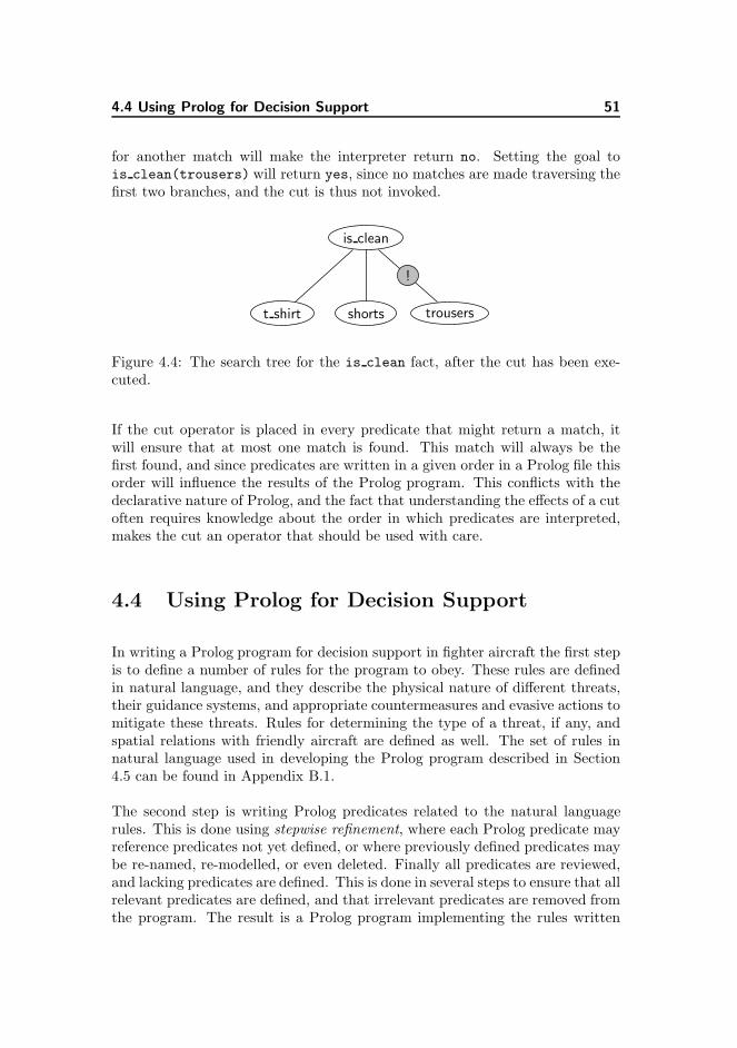
4.4 Using Prolog for Decision Support 51
for another match will make the interpreter return no. Setting the goal tois clean(trousers) will return yes, since no matches are made traversing thefirst two branches, and the cut is thus not invoked.
is clean
t shirt shorts trousers
!
Figure 4.4: The search tree for the is clean fact, after the cut has been exe-cuted.
If the cut operator is placed in every predicate that might return a match, itwill ensure that at most one match is found. This match will always be thefirst found, and since predicates are written in a given order in a Prolog file thisorder will influence the results of the Prolog program. This conflicts with thedeclarative nature of Prolog, and the fact that understanding the effects of a cutoften requires knowledge about the order in which predicates are interpreted,makes the cut an operator that should be used with care.
4.4 Using Prolog for Decision Support
In writing a Prolog program for decision support in fighter aircraft the first stepis to define a number of rules for the program to obey. These rules are definedin natural language, and they describe the physical nature of different threats,their guidance systems, and appropriate countermeasures and evasive actions tomitigate these threats. Rules for determining the type of a threat, if any, andspatial relations with friendly aircraft are defined as well. The set of rules innatural language used in developing the Prolog program described in Section4.5 can be found in Appendix B.1.
The second step is writing Prolog predicates related to the natural languagerules. This is done using stepwise refinement, where each Prolog predicate mayreference predicates not yet defined, or where previously defined predicates maybe re-named, re-modelled, or even deleted. Finally all predicates are reviewed,and lacking predicates are defined. This is done in several steps to ensure that allrelevant predicates are defined, and that irrelevant predicates are removed fromthe program. The result is a Prolog program implementing the rules written
52 The Prolog Approach
in the first step, or a relevant subset hereof, that will suggest actions to anyscenario described.
The Prolog program contains current warnings from the MWS and the RWR.Whenever a new warning occurs from either of these, the DSS should be con-sulted to see which action it proposes. Neither changes in the number or posi-tions of warnings from the RWR nor new warnings from the MWS, do necessarilyimply the presence of a new threat as stated in Section 3.5.2.
4.4.1 Assumptions
The program describes countermeasures and threats, which in substance behaveas described in Chapter 2. To ease the implementation of the Prolog program,some assumptions are made to the behaviour of threats and countermeasures.Also assumptions about descriptions of angles and distances are made.
The aircraft may be equipped with any combination of the following counter-measures: flares, DIRCM, chaff, jammer, and towed decoy. While the systemencompasses all of these countermeasures, they need to be installed on theaircraft, before the DSS will suggest actions involving them. The amount ofremaining flares, chaff, and decoys are relevant to the Prolog program. Thesenumbers are assumed updated in-flight by systems other than the DSS.
A warning from the RWR includes the detected threat type and the directiontoward the threat. Even though most RWRs can give an estimated distance tothe threat, this distance is not used by the program. For MWS warnings thetype of threat is not detected. Instead these warnings give the direction anddistance to a threat. Since a passive MWS (see Section 2.4) can not detect thedistance to a threat an active MWS is assumed.
All radar warnings represent threats, and friendly radar systems, informationof which could be given pre-mission, or supplied by an IFF, are not consideredan option.
If warnings from both the RWR and the MWS indicate that a threat occurs in agiven direction, this threat is likely to be RF guided, since this is the only kindof guidance detected by the RWR. If a MWS warning occurs at a given directionand no RWR warnings occur in that direction, then an IR guided missile isapproaching from that angle. An exception form this occurs when a friendlyaircraft is positioned in the direction given by the MWS warning, since this couldgive false MWS warnings. No other warnings are considered to be false. Whena RWR warning occurs, without a coinciding MWS warning, the RWR describes
4.4 Using Prolog for Decision Support 53
a tracking jammer, and not a RF guided missile.
Both breaklock zones (see Section 2.5.7) and directions to threats can be de-scribed in many ways. Even restricting the description to discrete values offersdifferent options, such as integer valued angles, maritime terminology (e.g. fore,beam, and aft), and aircraft parts (e.g. nose, wing, and tail). It is assumedthat describing angles using numbers between one and twelve is sufficient. Thenumbers relates to the positions on a clock, such that twelve o’clock describesthe direction straight ahead, six o’clock is in the opposite direction, and so on.
As with angles, different scales are used to describe distances. Altitude is oftendescribed using feet, while metres, kilometres, miles, or nautical miles are fre-quently used to describe longer, and mainly horizontal, distances. It is assumedthat the use of metres for all kind of distances does not affect the use of theprogram.
4.4.2 Available Information
The information available to the DSS can be divided into four different categories,based on the life span of the information. Here the categories are listed withdecreasing life spans:
Background Knowledge. Knowledge about missile types and guidance sys-tems are considered background knowledge. This type of information doesnot change very often, and it is considered static during a large numberof missions.
Mission Specific Knowledge. Before each mission, knowledge about the bat-tle scene, and positions and types of threats can be loaded into the system.This information may originate from intelligence sources.
Situation Description. Information about the locations of friendly aircraftmay continuously be received via a data link. This type of information isnecessary to recognize false missile warnings caused by friendly aircraft.
Warnings from on-board sensors. When a warning occurs from either theRWR or the MWS, information associated with this warning is fed to theDSS. RWR warnings give a direction to the threat, and information aboutwhat kind of threat it is estimated to be. MWS will also give a directionto the threat, combined with an estimated distance.
54 The Prolog Approach
4.5 The Prolog Program
The Prolog program developed implements most of the rules described in Ap-pendix B.1. The program is divided into two parts, where one part is concernedwith responding to actual warnings, and the other part responds to assump-tions about the environment, in which the aircraft is flying. A warning responseconsist of three parts: finding the set of appropriate countermeasures, selectingthe relevant program for each of these countermeasures, and calculating the ma-noeuvre that will bring the threats to the breaklock zone for the countermeasureselected.
For each warning the program may suggest more actions. All of these actionscomply with the rules set for the program, and they are not prioritized in anyway. A prioritization might be performed before the actions found are presentedto the pilot. The actions can be ordered according to an estimate of theirsurvivabilities, and if more actions offer the same survivability, the one requiringthe least effort from pilot and aircraft would have the highest priority.
Another use of the Prolog program is to query about e.g. the hostility of theenvironment, or the countermeasures to use for certain threats, etc.
4.5.1 Files
The Prolog program developed is described in seven files. Some of these files areassumed static during flight, while the contents of others files are dynamicallyupdated. The files are described below and their contents can be found inAppendix B. All files have the .pro extension. While this is not a necessaryextension of Prolog-files, it makes it easier to recognize the files as such.
dss.pro This file includes the main parts of the Prolog-based DSS. It includesrules for estimating and addressing the hostility of the environment, andfinding relevant countermeasures for the warnings given. The suggestionsof countermeasures depend on e.g. the altitude of the aircraft, the distanceto threats, and the availability of the countermeasures. It is assumed thatno new operational rules are given during flight, and the content of thisfile is thus considered static.
warnings.pro The current warnings are described here. Warnings from theMWS are described with an angle and a direction to the alleged incomingmissile, while RWR warnings are described by angle and type of threat.

4.5 The Prolog Program 55
Since warnings may occur and disappear at any time during flight thecontent of this file is highly dynamic.
current.pro The current description of the aircraft itself is provided in thisfile. This includes information about altitude, the amount of remainingexpendables, and the modes of available countermeasures. The position offriendly aircraft is also given in this file. As with warnings, the informationgiven in this file is highly dynamic.
mission.pro Details about the mission, the countermeasures available to thepilot, and a description of the estimated threat scenario are given in thisfile. This information is supposed to be given pre-mission, and the file canthus be considered static during the mission. If new information aboute.g. the positions and numbers of threats become available during flightit should be possible to update this file.
cm.pro For chaff and flares a number of different programs are available. Whichprogram to choose depends on the threat, the number of chaff or flaresremaining, the altitude, etc. These programs, as well as breaklock zonesfor different countermeasures, are described in this file, as are rules fordetermining whether the countermeasures are currently in effect. Nei-ther countermeasures nor their related programs are subjects to frequentchanges, and this file can be considered static.
threats.pro This file describes background knowledge about all threats thatmay be encountered, not just the threats expected in the current mission.It also describes what type of guidance systems missiles associated withthe threats use, and how to mitigate these guidance systems. This file isconsidered static.
util.pro This file contains functions for handling lists, writing messages to thescreen, and calculating manoeuvres between angles. It should be updatedonly if the DSS itself changes.
The file dss.pro includes all other files and it is thus the only file one needs toconsult to run the program. The facts and predicates described in the programare listed in Tables 4.1 and 4.2. When the current situation is described inthe files mission.pro, current.pro, and warnings.pro, the rule go (withoutarguments) can be invoked at the Prolog prompt. Most of the work is done inthe what to do function, and go only measures how long it takes to performwhat to do, and writes the result to the screen.
The program will return all feasible actions. This has the effect that warningswith more than one appropriate countermeasure will get actions recommendingeach of these, and countermeasures with more than one breaklock zone will berecommended with a manoeuvre to each of these zones.
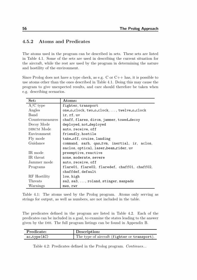
56 The Prolog Approach
4.5.2 Atoms and Predicates
The atoms used in the program can be described in sets. These sets are listedin Table 4.1. Some of the sets are used in describing the current situation forthe aircraft, while the rest are used by the program in determining the natureand hostility of the environment.
Since Prolog does not have a type check, as e.g. C or C++ has, it is possible touse atoms other than the ones described in Table 4.1. Doing this may cause theprogram to give unexpected results, and care should therefore be taken whene.g. describing scenarios.
Set: Atoms:A/C type fighter, transportAngles one o clock, two o clock, . . . , twelve o clock
Band ir, rf, uvCountermeasures chaff, flares, dircm, jammer, towed decoy
Decoy Mode deployed, not deployed
DIRCM Mode auto, receive, offEnvironment friendly, hostileFly mode take off, cruise, landingGuidance command, sarh, qas tvm, inertial, ir, aclos,
saclos, optical, laser beam rider, uvIR mode preemptive, reactiveIR threat none, moderate, severeJammer mode auto, receive, offPrograms flare01, flare02, flaredef, chaff01, chaff02,
chaffdef, defaultRF Hostility low, highThreats sa2, sa3, . . . , roland, stinger, manpadsWarnings mws, rwr
Table 4.1: The atoms used by the Prolog program. Atoms only serving asstrings for output, as well as numbers, are not included in the table.
The predicates defined in the program are listed in Table 4.2. Each of thepredicates can be included in a goal, to examine the states leading to the answergiven by the DSS. The full program listings can be found in Appendix B.
Predicate: Description:ac type(AC) The type of aircraft (fighter or transport).
Table 4.2: Predicates defined in the Prolog program. Continues...
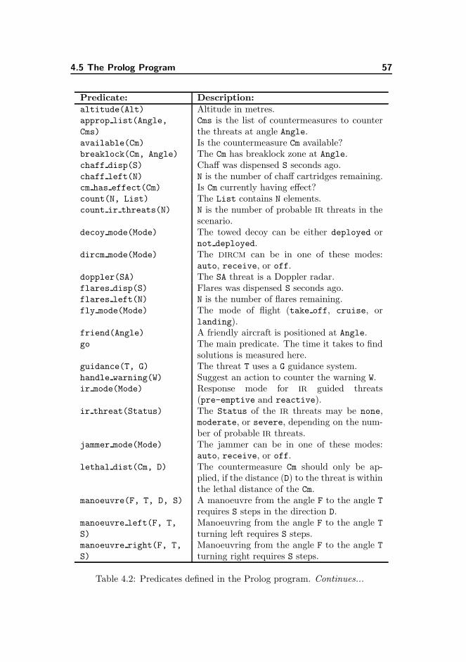
4.5 The Prolog Program 57
Predicate: Description:altitude(Alt) Altitude in metres.approp list(Angle,
Cms)
Cms is the list of countermeasures to counterthe threats at angle Angle.
available(Cm) Is the countermeasure Cm available?breaklock(Cm, Angle) The Cm has breaklock zone at Angle.chaff disp(S) Chaff was dispensed S seconds ago.chaff left(N) N is the number of chaff cartridges remaining.cm has effect(Cm) Is Cm currently having effect?count(N, List) The List contains N elements.count ir threats(N) N is the number of probable IR threats in the
scenario.decoy mode(Mode) The towed decoy can be either deployed or
not deployed.dircm mode(Mode) The DIRCM can be in one of these modes:
auto, receive, or off.doppler(SA) The SA threat is a Doppler radar.flares disp(S) Flares was dispensed S seconds ago.flares left(N) N is the number of flares remaining.fly mode(Mode) The mode of flight (take off, cruise, or
landing).friend(Angle) A friendly aircraft is positioned at Angle.go The main predicate. The time it takes to find
solutions is measured here.guidance(T, G) The threat T uses a G guidance system.handle warning(W) Suggest an action to counter the warning W.ir mode(Mode) Response mode for IR guided threats
(pre-emptive and reactive).ir threat(Status) The Status of the IR threats may be none,
moderate, or severe, depending on the num-ber of probable IR threats.
jammer mode(Mode) The jammer can be in one of these modes:auto, receive, or off.
lethal dist(Cm, D) The countermeasure Cm should only be ap-plied, if the distance (D) to the threat is withinthe lethal distance of the Cm.
manoeuvre(F, T, D, S) A manoeuvre from the angle F to the angle T
requires S steps in the direction D.manoeuvre left(F, T,
S)
Manoeuvring from the angle F to the angle T
turning left requires S steps.manoeuvre right(F, T,
S)
Manoeuvring from the angle F to the angle T
turning right requires S steps.
Table 4.2: Predicates defined in the Prolog program. Continues...

58 The Prolog Approach
Predicate: Description:memberof(M,List) M is a member of List.mitigates(B, Cm) Threats using guidance in the B band can be
mitigated using the countermeasure Cm.phys guidance(G, B) The guidance system G works within the band
B.prog(Cm, Prog) The countermeasure Cm can be activated using
the program Prog.proper cm(Angle, Cm) Cm is one of the countermeasures to be used
against threats at Angle.recommend action(W,
Cm, M, P)
The recommended action to the warning W
consists of a countermeasure Cm, a manoeuvreM, and a program P.
recommend cm(W, Cm) Cm is a recommended countermeasure countingthreats at the angle described in the warningW.
recommend man(W, Cm,
M)
The manoeuvre M, described by a directionand a number of steps, should accompany thecountermeasure Cm to counter threats at theangle described in the warning W.
rf hostility(H) Depending on the amount of probable RF
threats in the scenario, the RF hostility canbe either low or high.
safe altitude(B) The aircraft may fly at an altitude, wherethreats operating in the band B do not posea threat.
threat probable(SA) The presence of threat SA is considered prob-able.
turn left(X, Y) Angle Y is one step to the left of angle X.turn right(X, Y) Angle Y is one step to the right of angle X.warning(S, (Angle,
Data))
S indicates the sensor from which the warningcomes, and Angle gives the direction to thethreat. If S is mws the warning describes amissile, and the Data part gives the distance tothe missile. If S is rwr the Data part describesthe type of threat.
what to do This predicate will find actions related to allwarnings, and to the hostility of the environ-ment.
write cm(Cm, Prog) The recommended countermeasure Cm and theprogram Prog to use is written to the screen.
Table 4.2: Predicates defined in the Prolog program. Continues...
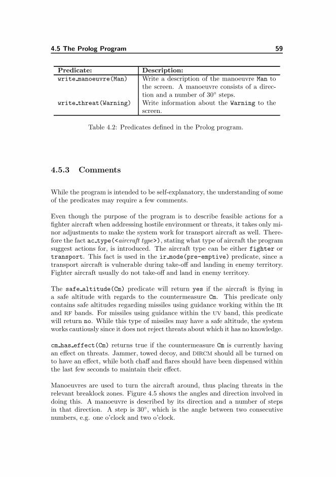
4.5 The Prolog Program 59
Predicate: Description:write manoeuvre(Man) Write a description of the manoeuvre Man to
the screen. A manoeuvre consists of a direc-tion and a number of 30◦ steps.
write threat(Warning) Write information about the Warning to thescreen.
Table 4.2: Predicates defined in the Prolog program.
4.5.3 Comments
While the program is intended to be self-explanatory, the understanding of someof the predicates may require a few comments.
Even though the purpose of the program is to describe feasible actions for afighter aircraft when addressing hostile environment or threats, it takes only mi-nor adjustments to make the system work for transport aircraft as well. There-fore the fact ac type(<aircraft type>), stating what type of aircraft the programsuggest actions for, is introduced. The aircraft type can be either fighter ortransport. This fact is used in the ir mode(pre-emptive) predicate, since atransport aircraft is vulnerable during take-off and landing in enemy territory.Fighter aircraft usually do not take-off and land in enemy territory.
The safe altitude(Cm) predicate will return yes if the aircraft is flying ina safe altitude with regards to the countermeasure Cm. This predicate onlycontains safe altitudes regarding missiles using guidance working within the IR
and RF bands. For missiles using guidance within the UV band, this predicatewill return no. While this type of missiles may have a safe altitude, the systemworks cautiously since it does not reject threats about which it has no knowledge.
cm has effect(Cm) returns true if the countermeasure Cm is currently havingan effect on threats. Jammer, towed decoy, and DIRCM should all be turned onto have an effect, while both chaff and flares should have been dispensed withinthe last few seconds to maintain their effect.
Manoeuvres are used to turn the aircraft around, thus placing threats in therelevant breaklock zones. Figure 4.5 shows the angles and direction involved indoing this. A manoeuvre is described by its direction and a number of stepsin that direction. A step is 30◦, which is the angle between two consecutivenumbers, e.g. one o’clock and two o’clock.
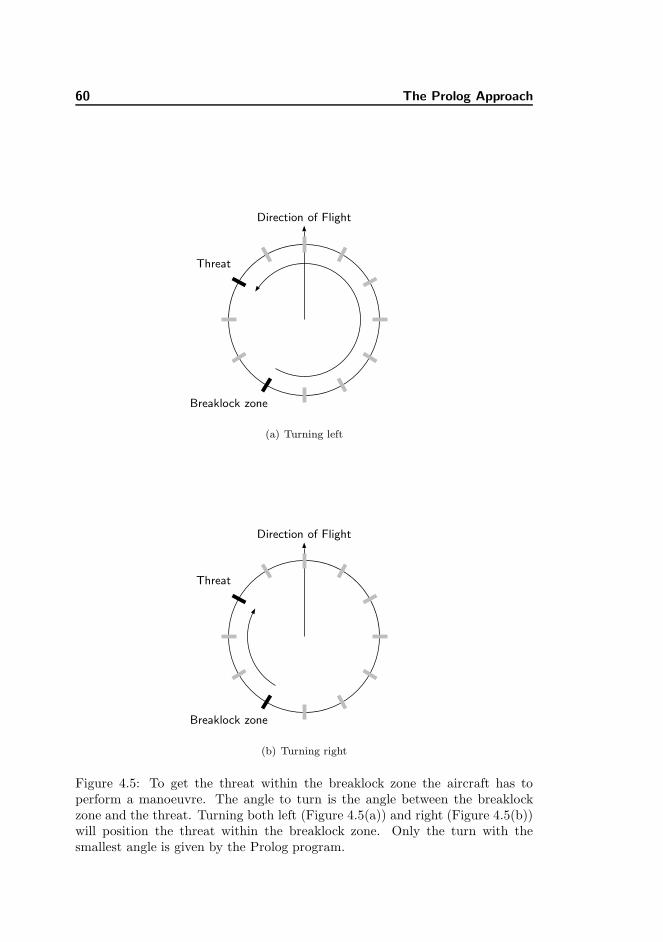
60 The Prolog Approach
Direction of Flight
Threat
Breaklock zone
(a) Turning left
Direction of Flight
Threat
Breaklock zone
(b) Turning right
Figure 4.5: To get the threat within the breaklock zone the aircraft has toperform a manoeuvre. The angle to turn is the angle between the breaklockzone and the threat. Turning both left (Figure 4.5(a)) and right (Figure 4.5(b))will position the threat within the breaklock zone. Only the turn with thesmallest angle is given by the Prolog program.
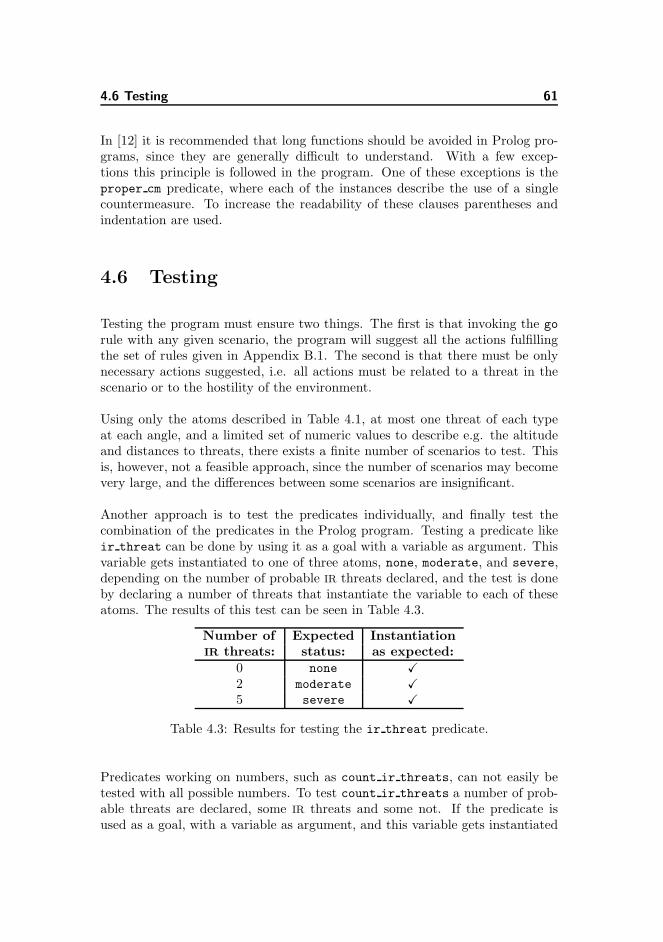
4.6 Testing 61
In [12] it is recommended that long functions should be avoided in Prolog pro-grams, since they are generally difficult to understand. With a few excep-tions this principle is followed in the program. One of these exceptions is theproper cm predicate, where each of the instances describe the use of a singlecountermeasure. To increase the readability of these clauses parentheses andindentation are used.
4.6 Testing
Testing the program must ensure two things. The first is that invoking the go
rule with any given scenario, the program will suggest all the actions fulfillingthe set of rules given in Appendix B.1. The second is that there must be onlynecessary actions suggested, i.e. all actions must be related to a threat in thescenario or to the hostility of the environment.
Using only the atoms described in Table 4.1, at most one threat of each typeat each angle, and a limited set of numeric values to describe e.g. the altitudeand distances to threats, there exists a finite number of scenarios to test. Thisis, however, not a feasible approach, since the number of scenarios may becomevery large, and the differences between some scenarios are insignificant.
Another approach is to test the predicates individually, and finally test thecombination of the predicates in the Prolog program. Testing a predicate likeir threat can be done by using it as a goal with a variable as argument. Thisvariable gets instantiated to one of three atoms, none, moderate, and severe,depending on the number of probable IR threats declared, and the test is doneby declaring a number of threats that instantiate the variable to each of theseatoms. The results of this test can be seen in Table 4.3.
Number of Expected InstantiationIR threats: status: as expected:
0 none X
2 moderate X
5 severe X
Table 4.3: Results for testing the ir threat predicate.
Predicates working on numbers, such as count ir threats, can not easily betested with all possible numbers. To test count ir threats a number of prob-able threats are declared, some IR threats and some not. If the predicate isused as a goal, with a variable as argument, and this variable gets instantiated
62 The Prolog Approach
according to the number of IR threats, the predicate works as intended. Forpredicates working on lists, the same problem occurs: not all lists can easily betested for, and a subset should be chosen. The predicate approp list is oneexample of such a predicate. If used as a goal, with the second argument beinga variable, the instantiation of this variable can be controlled to see whether thecountermeasures suggested are according to the set of rules.
The testing of all predicates is performed during the development of the Prologprogram. To test if the program itself behaves as expected, a number of scenariosare described, and the program is run with each of these scenarios as describedbelow.
4.6.1 Scenarios
Eight different scenarios are used in testing the DSS. These scenarios vary ingravity, from a single threat to a scenario where the number of threats probablyexceeds that of any real-world scenario. The last of these scenarios is constructedto be a worst case scenario, and it is included here to find the maximum runningtime of the DSS. While worse scenarios may be constructed it is assumed that noreal-world scenario will require more performance of the Prolog program thanthis. The scenarios are described in Table 4.4. If nothing else is mentionedin the description of a scenario the fighter aircraft will be equipped with allthe described countermeasures, the amounts of available expendables will behigh enough to perform any of the programs, and the aircraft is cruising at analtitude of 600 metres. The threats shown in the scenarios are also the threatsfound to be probable, described using the threat probable predicate.
Description: Scenario:Scenario 1
SA-2A single non-Doppler radar is positioned attwelve o’clock. No missile is detected.Scenario 2
SA-2
SA-3
SA-7
This scenario contains three threats, tworadar-based (SA-2 and SA-3), and a sin-gle threat with IR guidance (SA-7). Thethreats are all placed in front of the air-craft (eleven o’clock, twelve o’clock, andone o’clock). A missile is fired from theSA-7.
Table 4.4: Scenarios used for testing the Prolog based DSS. Con-tinues...
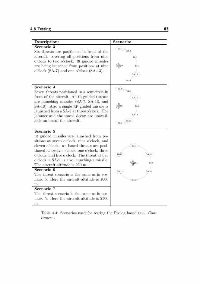
4.6 Testing 63
Description: Scenario:Scenario 3
SA-7SA-2
SA-3
SA-5
SA-13
SA-10
Six threats are positioned in front of theaircraft, covering all positions from nineo’clock to two o’clock. IR guided missilesare being launched from positions at nineo’clock (SA-7) and one o’clock (SA-13).
Scenario 4SA-7
SA-2
SA-18
SA-5
SA-10
SA-13SA-3
Seven threats positioned in a semicircle infront of the aircraft. All IR guided threatsare launching missiles (SA-7, SA-13, andSA-18). Also a single RF guided missile islaunched from a SA-3 at three o’clock. Thejammer and the towed decoy are unavail-able on-board the aircraft.
Scenario 5
SA-7
SA-18
SA-10
SA-3
SA-2
SA-5
SA-13
IR guided missiles are launched from po-sitions at seven o’clock, nine o’clock, andeleven o’clock. RF based threats are posi-tioned at twelve o’clock, one o’clock, threeo’clock, and five o’clock. The threat at fiveo’clock, a SA-2, is also launching a missile.The aircraft altitude is 250 m.Scenario 6The threat scenario is the same as in sce-nario 5. Here the aircraft altitude is 1000m.Scenario 7The threat scenario is the same as in sce-nario 5. Here the aircraft altitude is 2500m.
Table 4.4: Scenarios used for testing the Prolog based DSS. Con-tinues...
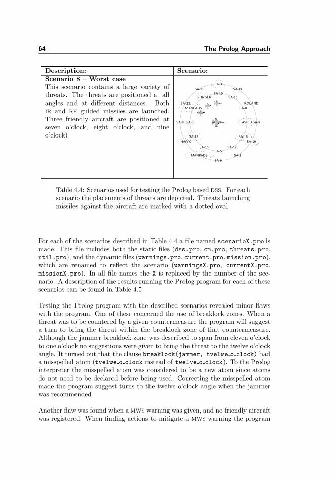
64 The Prolog Approach
Description: Scenario:Scenario 8 – Worst case
ASPID
SA-18
SA-12bSA-5
SA-10
SA-13
SA-3
MANPADS
STINGERSA-10
SA-15
SA-8
SA-5
SA-19
SA-2
SA-6
MANPADS
IHAWK
SA-8
SA-12
SA-11
SA-3
SA-19
ROLAND
This scenario contains a large variety ofthreats. The threats are positioned at allangles and at different distances. BothIR and RF guided missiles are launched.Three friendly aircraft are positioned atseven o’clock, eight o’clock, and nineo’clock)
Table 4.4: Scenarios used for testing the Prolog based DSS. For eachscenario the placements of threats are depicted. Threats launchingmissiles against the aircraft are marked with a dotted oval.
For each of the scenarios described in Table 4.4 a file named scenarioX.pro ismade. This file includes both the static files (dss.pro, cm.pro, threats.pro,util.pro), and the dynamic files (warnings.pro, current.pro, mission.pro),which are renamed to reflect the scenario (warningsX.pro, currentX.pro,missionX.pro). In all file names the X is replaced by the number of the sce-nario. A description of the results running the Prolog program for each of thesescenarios can be found in Table 4.5
Testing the Prolog program with the described scenarios revealed minor flawswith the program. One of these concerned the use of breaklock zones. When athreat was to be countered by a given countermeasure the program will suggesta turn to bring the threat within the breaklock zone of that countermeasure.Although the jammer breaklock zone was described to span from eleven o’clockto one o’clock no suggestions were given to bring the threat to the twelve o’clockangle. It turned out that the clause breaklock(jammer, tvelwe o clock) hada misspelled atom (tvelwe o clock instead of twelve o clock). To the Prologinterpreter the misspelled atom was considered to be a new atom since atomsdo not need to be declared before being used. Correcting the misspelled atommade the program suggest turns to the twelve o’clock angle when the jammerwas recommended.
Another flaw was found when a MWS warning was given, and no friendly aircraftwas registered. When finding actions to mitigate a MWS warning the program
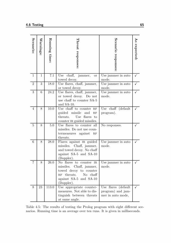
4.6 Testing 65
Scenario
:
Warn
ings:
Runnin
gtim
e:
Thre
at
resp
onse
s:
Scenario
resp
onse
s:
As
expecte
d:
1 1 7.1 Use chaff, jammer, ortowed decoy.
Use jammer in automode.
X
2 3 18.0 Use flares, chaff, jammer,or towed decoy.
Use jammer in automode.
X
3 6 24.2 Use flares, chaff, jammer,or towed decoy. Do notuse chaff to counter SA-5and SA-10.
Use jammer in automode.
X
4 8 10.0 Use chaff to counter RF
guided missile and RF
threats. Use flares tocounter IR guided missiles.
Use chaff (defaultprogram).
X
5 8 5.0 Use flares to counter allmissiles. Do not use coun-termeasures against RF
threats.
No responses. X
6 8 28.0 Flares against IR guidedmissiles. Chaff, jammer,and towed decoy. No chaffagainst SA-5 and SA-10(Doppler).
Use jammer in automode.
X
7 8 26.0 No flares to counter IR
missiles. Chaff, jammer,towed decoy to counterRF threats. No chaffagainst SA-5 and SA-10(Doppler).
Use jammer in automode.
X
8 23 113.0 Use appropriate counter-measures. Not able to dis-tinguish between threatsat same angle.
Use flares (defaultprogram) and jam-mer in auto mode,
X
Table 4.5: The results of testing the Prolog program with eight different sce-narios. Running time is an average over ten runs. It is given in milliseconds.
66 The Prolog Approach
first checks if a friendly aircraft is reported to be at the same angle and if sothe warning is neglected. If no friendly aircraft was registered the B-Prologinterpreter was not able to run. This may be an interpreter dependent errorsince other interpreters may just return no if a predicate has not been defined.The flaw was corrected by always defining a friend(none) clause, and theprogram can now be run by the B-Prolog interpreter.
As no more flaws were found the program returns expected responses to all of thescenarios. Appropriate countermeasures are suggested depending on the threats,the aircraft altitude, and the countermeasures available. Also responses to thescenario are as expected. They depend on the types and number of probablethreats in the scenario, and on the availability of countermeasures.
It is found that the number of warnings in the scenario description has someinfluence on the time it takes to run the Prolog program. The first scenariohas one warning only, and finding solutions to this is done in an average of7 milliseconds. Responses to the last scenario, having 23 warnings, are foundat an average of 113 milliseconds. Since four of the eight scenarios have eightwarnings, and the average time for finding solutions for these vary from 5 to28 milliseconds, it can not be concluded that the number of warnings alonedetermine the time it takes to find solutions to a given scenario.
4.7 Discussion
In developing the Prolog program, the first step was to describe a set of rulesfor the program to fulfil. During development, questions to these rules come up,and more rules may become necessary. Therefore the set of rules are not to beconsidered a static entity. The set will evolve in a number of iterations duringthe development of the program.
Some of the rules are expressed in such a way that they can be more or lessdirectly translated into Prolog predicates. Other rules have a more subtle formu-lation, which makes them more difficult to implement. The rule ”The jammerwill reveal the position of the aircraft” is an example of one such rule. Whileit is true, and relatively easy to implement, the implications of the rule on theProlog program are not obvious. A rule stating ”The jammer should only beactive in a non-severe environment if it mitigates a missile launched towards theaircraft”, would describe the same intention: the jammer should not be activeunless it makes a positive difference to the survivability. Implementing it in theprogram is just as easy.
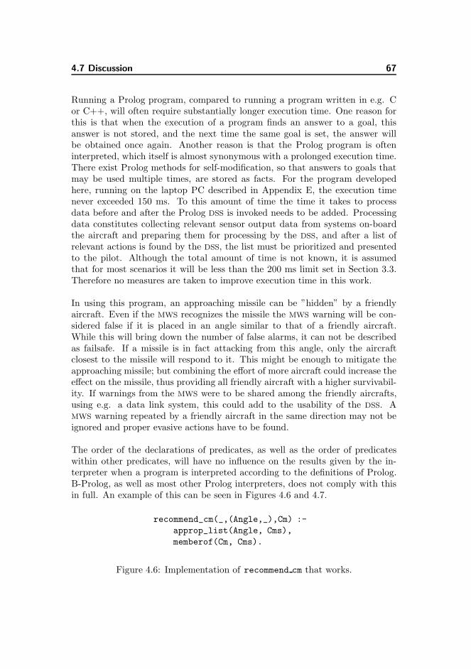
4.7 Discussion 67
Running a Prolog program, compared to running a program written in e.g. Cor C++, will often require substantially longer execution time. One reason forthis is that when the execution of a program finds an answer to a goal, thisanswer is not stored, and the next time the same goal is set, the answer willbe obtained once again. Another reason is that the Prolog program is ofteninterpreted, which itself is almost synonymous with a prolonged execution time.There exist Prolog methods for self-modification, so that answers to goals thatmay be used multiple times, are stored as facts. For the program developedhere, running on the laptop PC described in Appendix E, the execution timenever exceeded 150 ms. To this amount of time the time it takes to processdata before and after the Prolog DSS is invoked needs to be added. Processingdata constitutes collecting relevant sensor output data from systems on-boardthe aircraft and preparing them for processing by the DSS, and after a list ofrelevant actions is found by the DSS, the list must be prioritized and presentedto the pilot. Although the total amount of time is not known, it is assumedthat for most scenarios it will be less than the 200 ms limit set in Section 3.3.Therefore no measures are taken to improve execution time in this work.
In using this program, an approaching missile can be ”hidden” by a friendlyaircraft. Even if the MWS recognizes the missile the MWS warning will be con-sidered false if it is placed in an angle similar to that of a friendly aircraft.While this will bring down the number of false alarms, it can not be describedas failsafe. If a missile is in fact attacking from this angle, only the aircraftclosest to the missile will respond to it. This might be enough to mitigate theapproaching missile; but combining the effort of more aircraft could increase theeffect on the missile, thus providing all friendly aircraft with a higher survivabil-ity. If warnings from the MWS were to be shared among the friendly aircrafts,using e.g. a data link system, this could add to the usability of the DSS. AMWS warning repeated by a friendly aircraft in the same direction may not beignored and proper evasive actions have to be found.
The order of the declarations of predicates, as well as the order of predicateswithin other predicates, will have no influence on the results given by the in-terpreter when a program is interpreted according to the definitions of Prolog.B-Prolog, as well as most other Prolog interpreters, does not comply with thisin full. An example of this can be seen in Figures 4.6 and 4.7.
recommend_cm(_,(Angle,_),Cm) :-
approp_list(Angle, Cms),
memberof(Cm, Cms).
Figure 4.6: Implementation of recommend cm that works.
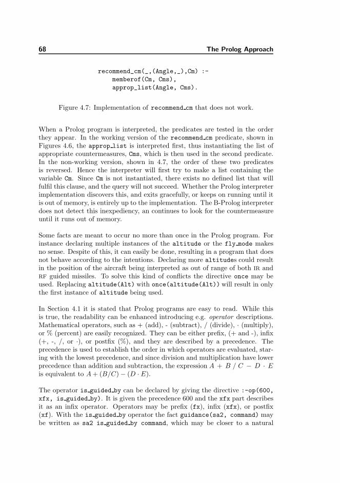
68 The Prolog Approach
recommend_cm(_,(Angle,_),Cm) :-
memberof(Cm, Cms),
approp_list(Angle, Cms).
Figure 4.7: Implementation of recommend cm that does not work.
When a Prolog program is interpreted, the predicates are tested in the orderthey appear. In the working version of the recommend cm predicate, shown inFigures 4.6, the approp list is interpreted first, thus instantiating the list ofappropriate countermeasures, Cms, which is then used in the second predicate.In the non-working version, shown in 4.7, the order of these two predicatesis reversed. Hence the interpreter will first try to make a list containing thevariable Cm. Since Cm is not instantiated, there exists no defined list that willfulfil this clause, and the query will not succeed. Whether the Prolog interpreterimplementation discovers this, and exits gracefully, or keeps on running until itis out of memory, is entirely up to the implementation. The B-Prolog interpreterdoes not detect this inexpediency, an continues to look for the countermeasureuntil it runs out of memory.
Some facts are meant to occur no more than once in the Prolog program. Forinstance declaring multiple instances of the altitude or the fly mode makesno sense. Despite of this, it can easily be done, resulting in a program that doesnot behave according to the intentions. Declaring more altitudes could resultin the position of the aircraft being interpreted as out of range of both IR andRF guided missiles. To solve this kind of conflicts the directive once may beused. Replacing altitude(Alt) with once(altitude(Alt)) will result in onlythe first instance of altitude being used.
In Section 4.1 it is stated that Prolog programs are easy to read. While thisis true, the readability can be enhanced introducing e.g. operator descriptions.Mathematical operators, such as + (add), - (subtract), / (divide), · (multiply),or % (percent) are easily recognized. They can be either prefix, (+ and -), infix(+, -, /, or ·), or postfix (%), and they are described by a precedence. Theprecedence is used to establish the order in which operators are evaluated, star-ing with the lowest precedence, and since division and multiplication have lowerprecedence than addition and subtraction, the expression A + B / C − D · Eis equivalent to A + (B/C)− (D · E).
The operator is guided by can be declared by giving the directive :-op(600,
xfx, is guided by). It is given the precedence 600 and the xfx part describesit as an infix operator. Operators may be prefix (fx), infix (xfx), or postfix(xf). With the is guided by operator the fact guidance(sa2, command) maybe written as sa2 is guided by command, which may be closer to a natural
4.8 Conclusion 69
language description of the guidance relation.
4.8 Conclusion
Developing a DSS prototype using Prolog is relatively easy. Based on rules statedby experts in the EW domain simple Prolog predicates can be developed withlittle effort. Combining all the rules translated from formulations in naturallanguage into one working Prolog program requires a little more effort. Theconcept of having the program perform two tasks, one finding proper responsesto the environment and one handling warnings from RWR and MWS, is notevident from the original set of rules.
While the concept of imperative programming seems intuitive, it may be dif-ficult to adjust to for a programmer used to imperative programming. Someknowledge about imperative programming may prove useful when programmingProlog, e.g. to find out why a Prolog program runs out of memory, when theorder of clauses is not set right.
Having a fixed set of rules to build the DSS from may not be the best foundationto build upon. As the development of the Prolog program progress the set ofrules must be updated to reflect new requirements to the knowledge gained fromthe rules.
In a DSS the use of Prolog will narrow the set of possible actions. While this mayhelp the pilot deciding on the actions to actually perform, it is not guaranteedthat action chosen will give the best survivability possible. Through his trainingthe pilot will have learned the rules from which the DSS infer actions, andtherefore an experienced pilot may not benefit as much from the DSS as a rookiewould. Since the hostile environment changes from one theatre to another, andthe tactics to follow are constantly evolving, even the best skilled pilot canbenefit from the presence of a Prolog based DSS, provided it is being frequentlyupdated.
Usually Prolog programs are considered slow. The Prolog program described inthis chapter performs relatively fast, and solutions are found within the stated200 millisecond limit. Adding to the usability of the program is likely to slowdown the performance of it, and a satisfactory trade-off between usability andperformance must be found.

70 The Prolog Approach
Chapter 5
The Bayesian Network
Approach
This chapter describes the use of a Bayesian Network (BN) as a method forevaluating actions for a fighter pilot to perform when a threat occurs. It de-scribes the basic theory of BN and why the technique may be an appropriateapproach in designing a DSS for fighter pilots. The process of constructing a BN
using the HUGIN tool is described. HUGIN offers a graphical user interface forthe construction of the network [7, 28] and details on HUGIN can be found inAppendix E.
The model developed gives the probability of the survival of the aircraft de-pending on the state of the world surrounding the aircraft, knowledge aboutan emerging threat, and a selection of possible actions for the pilot to take. Inbuilding the model, part of the work may seem both cumbersome and complex.Hence two methods to do these parts in a semi-automatic way are explored anddescribed as well.
BNs are used in a wide range of areas, including vision, natural language process-ing, robot navigation, planning, and machine learning [17]. In relevant literatureBNs are also referred to as belief networks, Bayesian belief networks, Bayesiandependency nets, or causal probabilistic networks. The name decision graphs,as used in section 5.2.6, refers to BNs containing utility and/or decision nodes
72 The Bayesian Network Approach
[22]. These are also known as influence diagrams [17]. See [13, 21, 22, 23, 34]for more in-depth description of BN and probabilistic reasoning.
5.1 Motivation
A decision support system on-board an aircraft will depend on information froma number of sources. The uncertainty of some information (such as the kindand amount of expendables on-board the aircraft, the pattern in which they willbe dispensed, and the angle in which they will depart from the aircraft) maybe considered negligible. Information about the kind of missiles the aircraftis likely to encounter may be obtained from intelligence sources, and shouldbe considered with some degree of uncertainty. Finally, data from on-boardwarning systems, giving angle, distance, and speed between the aircraft and anincoming missile, must be considered with high degrees of uncertainty. Incorrector incomplete data may be all the DSS initially has to support its decisions.
Since the sensors on-board the aircraft do not give an accurate image of the worldsurrounding it, using a BN to model this world seems a plausible approach asa BN can deal with the probabilities of e.g. the sensors being wrong and thecountermeasures not working as intended.
5.2 Basic Theory
A BN consists of a set of random variables, each variable having a number ofmutually exclusive states (at least two), and the variable can be in any one of itsstates with a given probability. It can be depicted as a directed acyclic graph,G = (V, E), with V being the set of variables shown as nodes in the graph, andthe set of directed edges between nodes, E, indicating dependencies betweenthem. Changes in states of some variables may cause changes in states of othervariables. The strengths of dependencies between variables are represented intables named dependency tables, conditional probability tables, or potential tables[22, 34]. In this work the term dependency table is used. For nodes withoutancestors, the dependency tables contain unconditional probabilities.
Relations between nodes in a BN are depicted using arrows. If A and B arevariables in the same network modelling a given domain an edge from B toA indicates that changes in the probabilities of the states in B may result inchanges in the probabilities of states in A. A is then said to be a child of B,and B is a parent of A (see Figure 5.1). A variable can have a number of both
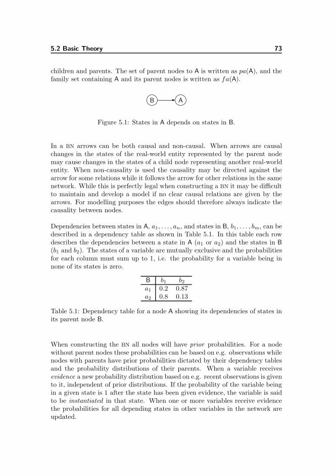
5.2 Basic Theory 73
children and parents. The set of parent nodes to A is written as pa(A), and thefamily set containing A and its parent nodes is written as fa(A).
B A
Figure 5.1: States in A depends on states in B.
In a BN arrows can be both causal and non-causal. When arrows are causalchanges in the states of the real-world entity represented by the parent nodemay cause changes in the states of a child node representing another real-worldentity. When non-causality is used the causality may be directed against thearrow for some relations while it follows the arrow for other relations in the samenetwork. While this is perfectly legal when constructing a BN it may be difficultto maintain and develop a model if no clear causal relations are given by thearrows. For modelling purposes the edges should therefore always indicate thecausality between nodes.
Dependencies between states in A, a1, . . . , an, and states in B, b1, . . . , bm, can bedescribed in a dependency table as shown in Table 5.1. In this table each rowdescribes the dependencies between a state in A (a1 or a2) and the states in B(b1 and b2). The states of a variable are mutually exclusive and the probabilitiesfor each column must sum up to 1, i.e. the probability for a variable being innone of its states is zero.
B b1 b2
a1 0.2 0.87a2 0.8 0.13
Table 5.1: Dependency table for a node A showing its dependencies of states inits parent node B.
When constructing the BN all nodes will have prior probabilities. For a nodewithout parent nodes these probabilities can be based on e.g. observations whilenodes with parents have prior probabilities dictated by their dependency tablesand the probability distributions of their parents. When a variable receivesevidence a new probability distribution based on e.g. recent observations is givento it, independent of prior distributions. If the probability of the variable beingin a given state is 1 after the state has been given evidence, the variable is saidto be instantiated in that state. When one or more variables receive evidencethe probabilities for all depending states in other variables in the network areupdated.
74 The Bayesian Network Approach
The nomenclature used in this chapter has been collected in Table 5.2.
A, B Nodes in the BN
ai, bj States of a nodepa(A) The set of parents to nodes in the set Afa(A) The family set including A and its parentsP (a) The probability of the state aA⊥B|C A and B are d-separated given evidence to C
Table 5.2: Nomenclature for Bayesian networks.
5.2.1 Probability Calculations
The probability of A being in state ai is written as P (A = ai). When thevariable involved is clearly defined by the context the form P (ai) is used. Theprobability of A being in state ai depending on B being in state bj is written asP (A = ai|B = bj) (or P (ai|bj) for short).
For doing probability calculations the fundamental rule is given by:
P (ai|bj)P (bj) = P (ai, bj). (5.1)
Here ai, bj means that A is in state ai and B is in state bj. Since P (ai|bj)P (bj) =P (ai, bj) = P (bj|ai)P (ai) the following rule is formulated:
P (bj |ai) =P (ai|bj)P (bj)
P (ai). (5.2)
This rule is known as Baye’s Rule1 and it is fundamental to the use of Bayesiannetworks. The probability P (ai|bj) clearly indicates that the value of A dependson the value of B. If the value of A is known, this probability also indicates someknowledge about the value of B. P (ai|bj) is thus often referred to as the likelihoodof bj given ai and it is written as L(bj|ai).
The HUGIN software uses potentials instead of probabilities. A potential can beany non-negative real number. The potential distribution for a given variablecan be turned into a probability distribution by normalization. Let A be avariable with n states, and let π(ai) be the potential of the ith state of A. Theprobability P (ai) of A being in the state ai is then given by
P (ai) =π(ai)Pn
j=1 π(aj).
1The rule is named after the Presbyterian minister and mathematician Thomas Bayes,1702 – 1761, who came up with the formulation ”A is known given knowledge about B”[3].
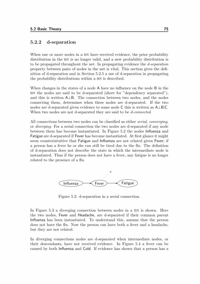
5.2 Basic Theory 75
5.2.2 d-separation
When one or more nodes in a BN have received evidence, the prior probabilitydistribution in the BN is no longer valid, and a new probability distribution isto be propagated throughout the net. In propagating evidence the d-separationproperty between pairs of nodes in the net is vital. This section gives the defi-nition of d-separation and in Section 5.2.5 a use of d-separation in propagatingthe probability distributions within a BN is described.
When changes in the states of a node A have no influence on the node B in theBN the nodes are said to be d-separated (short for ”dependency separated”),and this is written A⊥B. The connection between two nodes, and the nodesconnecting them, determines when these nodes are d-separated. If the twonodes are d-separated given evidence to some node C this is written as A⊥B|C.When two nodes are not d-separated they are said to be d-connected.
All connections between two nodes can be classified as either serial, converging,or diverging. For a serial connection the two nodes are d-separated if any nodebetween them has become instantiated. In Figure 5.2 the nodes Influenza andFatigue are d-separated if Fever has become instantiated. At first glance it mightseem counterintuitive that Fatigue and Influenza are not related given Fever; ifa person has a fever he or she can still be tired due to the flu. The definitionof d-separation does not describe the state in which the intermediate node isinstantiated. Thus if the person does not have a fever, any fatigue is no longerrelated to the presence of a flu.
Influenza Fever Fatigue
e
Figure 5.2: d-separation in a serial connection.
In Figure 5.3 a diverging connection between nodes in a BN is shown. Herethe two nodes, Fever and Headache, are d-separated if their common parentInfluenza has been instantiated. To understand this, assume that the persondoes not have the flu. Now the person can have both a fever and a headache,but they are not related.
In diverging connections nodes are d-separated when intermediate nodes, ortheir descendants, have not received evidence. In Figure 5.4 a fever can becaused by both Influenza and Cold. If evidence has shown that a person has a
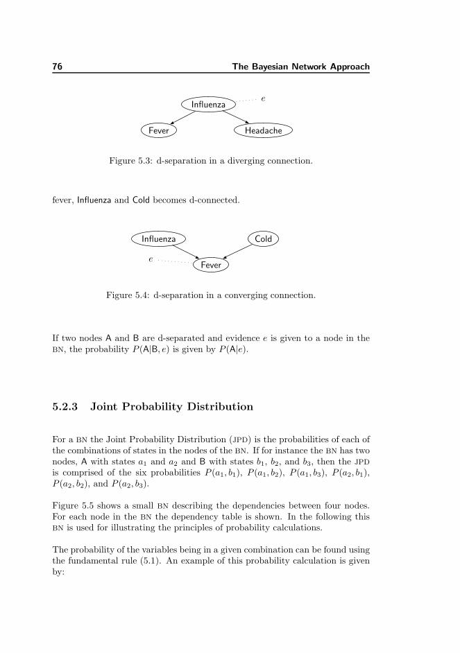
76 The Bayesian Network Approach
Fever
Influenza
Headache
e
Figure 5.3: d-separation in a diverging connection.
fever, Influenza and Cold becomes d-connected.
Influenza
Fever
Cold
e
Figure 5.4: d-separation in a converging connection.
If two nodes A and B are d-separated and evidence e is given to a node in theBN, the probability P (A|B, e) is given by P (A|e).
5.2.3 Joint Probability Distribution
For a BN the Joint Probability Distribution (JPD) is the probabilities of each ofthe combinations of states in the nodes of the BN. If for instance the BN has twonodes, A with states a1 and a2 and B with states b1, b2, and b3, then the JPD
is comprised of the six probabilities P (a1, b1), P (a1, b2), P (a1, b3), P (a2, b1),P (a2, b2), and P (a2, b3).
Figure 5.5 shows a small BN describing the dependencies between four nodes.For each node in the BN the dependency table is shown. In the following thisBN is used for illustrating the principles of probability calculations.
The probability of the variables being in a given combination can be found usingthe fundamental rule (5.1). An example of this probability calculation is givenby:
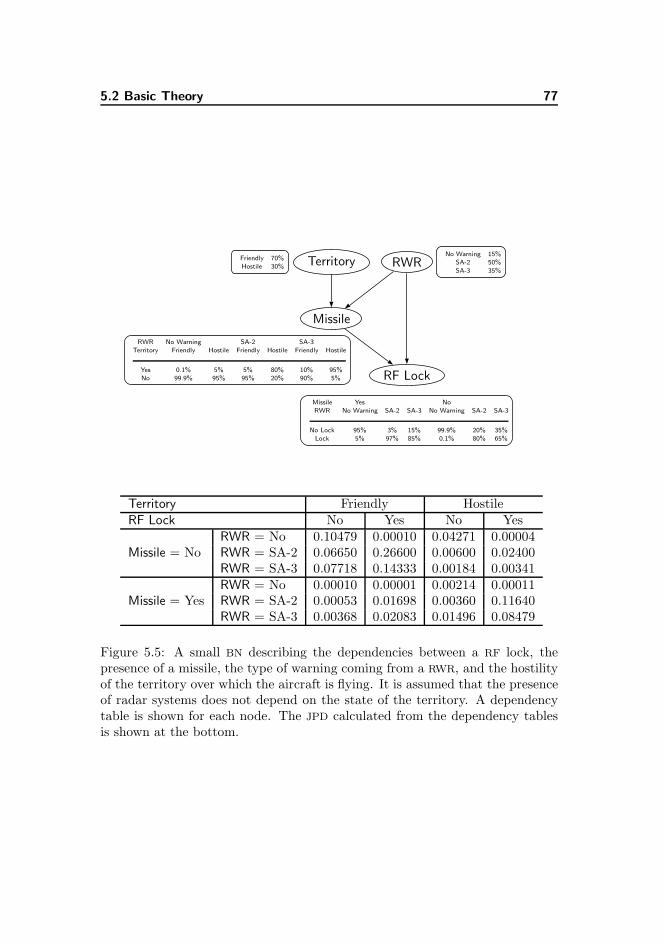
5.2 Basic Theory 77
Friendly 70%
Hostile 30% TerritoryNo Warning 15%
SA-2 50%
SA-3 35%RWR
RWR No Warning SA-2 SA-3
Territory Friendly Hostile Friendly Hostile Friendly Hostile
Yes 0.1% 5% 5% 80% 10% 95%
No 99.9% 95% 95% 20% 90% 5%
Missile
Missile Yes No
RWR No Warning SA-2 SA-3 No Warning SA-2 SA-3
No Lock 95% 3% 15% 99.9% 20% 35%
Lock 5% 97% 85% 0.1% 80% 65%
RF Lock
Territory Friendly HostileRF Lock No Yes No Yes
Missile = NoRWR = No 0.10479 0.00010 0.04271 0.00004RWR = SA-2 0.06650 0.26600 0.00600 0.02400RWR = SA-3 0.07718 0.14333 0.00184 0.00341
Missile = YesRWR = No 0.00010 0.00001 0.00214 0.00011RWR = SA-2 0.00053 0.01698 0.00360 0.11640RWR = SA-3 0.00368 0.02083 0.01496 0.08479
Figure 5.5: A small BN describing the dependencies between a RF lock, thepresence of a missile, the type of warning coming from a RWR, and the hostilityof the territory over which the aircraft is flying. It is assumed that the presenceof radar systems does not depend on the state of the territory. A dependencytable is shown for each node. The JPD calculated from the dependency tablesis shown at the bottom.
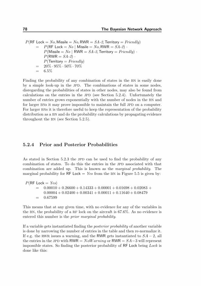
78 The Bayesian Network Approach
P (RF Lock = No, Missile = No, RWR = SA-2, Territory = Friendly)= P (RF Lock = No | Missile = No, RWR = SA-2) ·
P (Missile = No | RWR = SA-2, Territory = Friendly) ·P (RWR = SA-2) ·P (Territory = Friendly)
= 20% · 95% · 50% · 70%= 6.5%
Finding the probability of any combination of states in the BN is easily doneby a simple look-up in the JPD. The combinations of states in some nodes,disregarding the probabilities of states in other nodes, may also be found fromcalculations on the entries in the JPD (see Section 5.2.4). Unfortunately thenumber of entries grows exponentially with the number of nodes in the BN andfor larger BNs it may prove impossible to maintain the full JPD on a computer.For larger BNs it is therefore useful to keep the representation of the probabilitydistribution as a BN and do the probability calculations by propagating evidencethroughout the BN (see Section 5.2.5).
5.2.4 Prior and Posterior Probabilities
As stated in Section 5.2.3 the JPD can be used to find the probability of anycombination of states. To do this the entries in the JPD associated with thatcombination are added up. This is known as the marginal probability. Themarginal probability for RF Lock = Yes from the BN in Figure 5.5 is given by:
P (RF Lock = Yes)= 0.00010 + 0.26600 + 0.14333 + 0.00001 + 0.01698 + 0.02083 +
0.00004 + 0.02400 + 0.00341 + 0.00011 + 0.11640 + 0.08479= 0.67599
This means that at any given time, with no evidence for any of the variables inthe BN, the probability of a RF lock on the aircraft is 67.6%. As no evidence isentered this number is the prior marginal probability.
If a variable gets instantiated finding the posterior probability of another variableis done by narrowing the number of entries in the table and then re-normalize it.If e.g. the RWR issues a warning, and the RWR gets instantiated to SA− 2, allthe entries in the JPD with RWR = NoWarning or RWR = SA−3 will representimpossible states. So finding the posterior probability of RF Lock being Lock isdone like this:
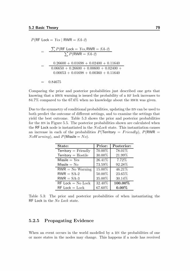
5.2 Basic Theory 79
P (RF Lock = Yes | RWR = SA-2)
=
PP (RF Lock = Yes, RWR = SA-2)P
P (RWR = SA-2)
=0.26600 + 0.01698 + 0.02400 + 0.11640
0.06650 + 0.26600 + 0.00600 + 0.02400 +0.00053 + 0.01698 + 0.00360 + 0.11640
= 0.84675
Comparing the prior and posterior probabilities just described one gets thatknowing that a RWR warning is issued the probability of a RF lock increases to84.7% compared to the 67.6% when no knowledge about the RWR was given.
Due to the symmetry of conditional probabilities, updating the BN can be used toboth predict the outcome of different settings, and to examine the settings thatyield the best outcome. Table 5.3 shows the prior and posterior probabilitiesfor the BN in Figure 5.5. The posterior probabilities shown are calculated whenthe RF Lock node is instantiated in the NoLock state. This instantiation causesan increase in each of the probabilities P (Territory = Friendly), P (RWR =NoWarning), and P (Missile = No).
State: Prior: Posterior:Territory = Friendly 70.00% 78.01%Territory = Hostile 30.00% 21.99%Missile = Yes 26.41% 7.72%Missile = No 73.59% 92.28%RWR = No Warning 15.00% 46.21%RWR = SA-2 50.00% 23.65%RWR = SA-3 35.00% 30.14%RF Lock = No Lock 32.40% 100.00%RF Lock = Lock 67.60% 0.00%
Table 5.3: The prior and posterior probabilities of when instantiating theRF Lock in the No Lock state.
5.2.5 Propagating Evidence
When an event occurs in the world modelled by a BN the probabilities of oneor more states in the nodes may change. This happens if a node has received
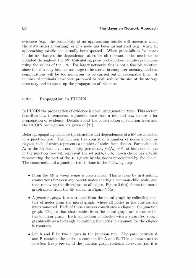
80 The Bayesian Network Approach
evidence (e.g. the probability of an approaching missile will increases whenthe MWS issues a warning) or if a node has been instantiated (e.g. when anapproaching missile has actually been spotted). When probabilities for statesin the BN changes the dependency tables for all relevant nodes needs to beupdated throughout the BN. Calculating prior probabilities can always be doneusing the values of the JPD. For larger networks this is not a feasible solutionsince the JPD may become too large to be stored in computer memory, and thecomputations will be too numerous to be carried out in reasonable time. Anumber of methods have been proposed to both reduce the size of the storagenecessary and to speed up the propagation of evidence.
5.2.5.1 Propagation in HUGIN
In HUGIN the propagation of evidence is done using junction trees. This sectiondescribes how to construct a junction tree from a BN, and how to use it forpropagation of evidence. Details about the construction of junction trees andthe HUGIN propagation are given in [21].
Before propagating evidence the structure and dependencies of a BN are collectedin a junction tree. The junction tree consist of a number of nodes known ascliques, each of which represents a number of nodes from the BN. For each nodeAi in the BN that has a non-empty parent set, pa(Ai) 6= ∅, at least one cliquein the junction tree will represent the set pa(Ai) ∪ Ai. Each clique has a tablerepresenting the part of the JPD given by the nodes represented by the clique.The construction of a junction tree is done in the following steps:
• From the BN a moral graph is constructed. This is done by first addingconnections between any parent nodes sharing a common child node, andthen removing the directions on all edges. Figure 5.6(b) shows the moralgraph made from the BN shown in Figure 5.6(a).
• A junction graph is constructed from the moral graph by collecting clus-ters of nodes from the moral graph, where all nodes in the clusters areinterconnected. Each of these clusters constitutes a clique in the junctiongraph. Cliques that share nodes from the moral graph are connected inthe junction graph. Each connection is labelled with a separator, showngraphically as a rectangle containing the nodes in common for the cliquesit connects.
• Let A and B be two cliques in the junction tree. The path between Aand B contains the nodes in common for A and B. This is known as thejunction tree property. If the junction graph contains no cycles (i.e. it is
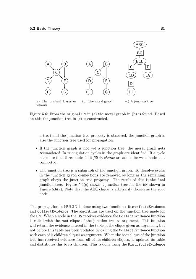
5.2 Basic Theory 81
A B
C
D E
F G
(a) The original Bayesiannetwork
A B
C
D E
F G
(b) The moral graph
ABC
BC
BCE
C
CD
E
EG
D
DF
(c) A junction tree
Figure 5.6: From the original BN in (a) the moral graph in (b) is found. Basedon this the junction tree in (c) is constructed.
a tree) and the junction tree property is observed, the junction graph isalso the junction tree used for propagation.
• If the junction graph is not yet a junction tree, the moral graph getstriangulated. In triangulation cycles in the graph are identified. If a cyclehas more than three nodes in it fill-in chords are added between nodes notconnected.
• The junction tree is a subgraph of the junction graph. To dissolve cyclesin the junction graph connections are removed as long as the remaininggraph obeys the junction tree property. The result of this is the finaljunction tree. Figure 5.6(c) shows a junction tree for the BN shown inFigure 5.6(a). Note that the ABC clique is arbitrarily chosen as the rootnode.
The propagation in HUGIN is done using two functions: DistributeEvidence
and CollectEvidence. The algorithms are used on the junction tree made forthe BN. When a node in the BN receives evidence the CollectEvidence functionis called with the root clique of the junction tree as argument. This functionwill return the evidence entered in the table of the clique given as argument, butnot before this table has been updated by calling the CollectEvidence functionwith each of is children cliques as argument. When the root clique of the junctiontree has received evidence from all of its children cliques, it updates its tableand distributes this to its children. This is done using the DistributeEvidence
82 The Bayesian Network Approach
function, which is used recursively throughout the junction tree. The resultingtables of the cliques now contain the updated probability distribution of the BN.
5.2.6 Decision Graphs
When using a BN for decision support a number of combinations of states havingreceived evidence can be compared. In this comparison each combination can beassociated with a scalar value, and the best combination will be the one yieldingthe highest/lowest value. If the BN is to be used in a DSS for fighter pilots thevalue to compare solutions by may be the probability of the aircraft survivingan attack (PS).
In associating a BN with a scalar value two types of nodes are introduced:decision nodes and utility nodes. Adding a node of either of these types to aBN makes it a Decision Graph (DG) [22], also known as an influence diagram[23]. Graphically decision nodes are shown as rectangular and utility nodes arediamond-shaped. A DG showing both decision and utility nodes can be seenin Figure 5.7. In a BN each node represents a variable. For a DG this is notthe case since neither action nor utility nodes represent variables in the domainmodelled.
Decision nodes represent actions in the network, and they have no dependencytables. Changes in the state of a decision node may influence the probabilitydistribution in ordinary nodes, while there is no influence the other way around.
The utility nodes represents additive contributions to the Expected Utility (EU)of the BN. The EU for a DG is the measure that is sought optimised. It mayhave a unit and all contributions to it stem from utility nodes. Each utility nodeis drawn with incoming lines from the nodes that may influence the outcomeof that node. Where ordinary nodes have a dependency table a utility nodehas a table showing the contribution by each combination of states in its parentnodes. Note that this contribution may be negative, e.g. representing a cost ina total turnover.
The DG in 5.7 was constructed using HUGIN. It models the situation of an Un-manned Aerial Vehicle (UAV) (cost price $100,000) flying over enemy territory.The UAV has been equipped with a flare dispenser and the DG can be used tocalculate the expected utility depending on whether or not flares are dispensedin a given situation. The EU is the sum of two terms, one concerned with theprice of dispensing flares ($1,000 per dispensing), and one concerned with theexpenses related to a possible UAV crash. With e being the evidence given tothe nodes IR Lock and Hit, and C being the cost of dispensing flares, the EU is
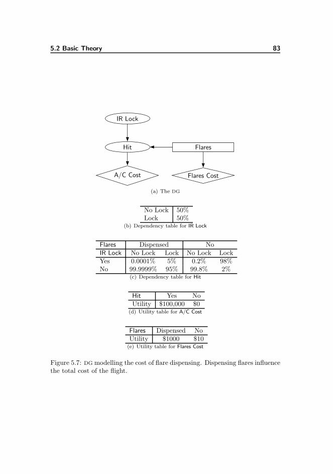
5.2 Basic Theory 83
IR Lock
Hit Flares
A/C Cost Flares Cost
(a) The DG
No Lock 50%Lock 50%
(b) Dependency table for IR Lock
Flares Dispensed NoIR Lock No Lock Lock No Lock LockYes 0.0001% 5% 0.2% 98%No 99.9999% 95% 99.8% 2%
(c) Dependency table for Hit
Hit Yes NoUtility $100,000 $0
(d) Utility table for A/C Cost
Flares Dispensed NoUtility $1000 $10
(e) Utility table for Flares Cost
Figure 5.7: DG modelling the cost of flare dispensing. Dispensing flares influencethe total cost of the flight.
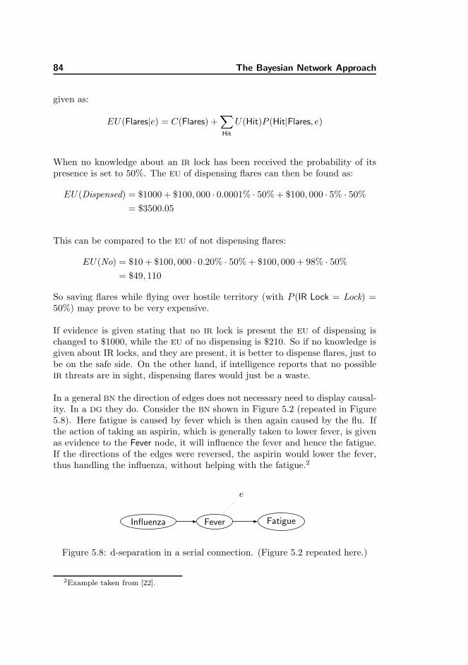
84 The Bayesian Network Approach
given as:
EU(Flares|e) = C(Flares) +XHit
U(Hit)P (Hit|Flares, e)
When no knowledge about an IR lock has been received the probability of itspresence is set to 50%. The EU of dispensing flares can then be found as:
EU(Dispensed) = $1000 + $100, 000 · 0.0001% · 50% + $100, 000 · 5% · 50%
= $3500.05
This can be compared to the EU of not dispensing flares:
EU(No) = $10 + $100, 000 · 0.20% · 50% + $100, 000 + 98% · 50%
= $49, 110
So saving flares while flying over hostile territory (with P (IR Lock = Lock) =50%) may prove to be very expensive.
If evidence is given stating that no IR lock is present the EU of dispensing ischanged to $1000, while the EU of no dispensing is $210. So if no knowledge isgiven about IR locks, and they are present, it is better to dispense flares, just tobe on the safe side. On the other hand, if intelligence reports that no possibleIR threats are in sight, dispensing flares would just be a waste.
In a general BN the direction of edges does not necessary need to display causal-ity. In a DG they do. Consider the BN shown in Figure 5.2 (repeated in Figure5.8). Here fatigue is caused by fever which is then again caused by the flu. Ifthe action of taking an aspirin, which is generally taken to lower fever, is givenas evidence to the Fever node, it will influence the fever and hence the fatigue.If the directions of the edges were reversed, the aspirin would lower the fever,thus handling the influenza, without helping with the fatigue.2
Influenza Fever Fatigue
e
Figure 5.8: d-separation in a serial connection. (Figure 5.2 repeated here.)
2Example taken from [22].
5.2 Basic Theory 85
5.2.7 Utility Scale
The EU is the sum of utilities from all utility nodes in the BN. Therefore it isnecessary for utilities to have a common unit. In maximising profit or minimisingcost a monetary unit will be adequate, while the unit to use in other cases maybe less obvious. For a company some actions may result in a momentary higherincome, while decreasing the customer satisfaction. In the long haul this maylead to a loss of customers, thus decreasing the turnover. In a situation likethis the EU should be measured using a utility scale, weighing both income andcustomer satisfaction.
Using a DG for decision support for fighter pilots will also require an appropriateutility scale. Having the probability of survival, PS , defining the scale may beless opportune since this probability depends on combinations of actions. Thismeans that the values of the utility nodes does not depend solely on states indiscrete nodes, and therefore the utility nodes cannot be correctly connectedto any nodes in the DG. To remedy this, a single node to connect a utilitynode to can be constructed. This node will contain all combinations of statesfrom the nodes on which the survivability depends. While this is possible theconstruction of such a node is cumbersome and the ability for using a DG formodelling the domain is weakened.
If survivability is represented as a score, where mitigating a threat would have apositive influence on the score, while e.g. using expendables or making the threatfocus on the aircraft by turning on the jammer when this is not necessary, wouldhave a negative influence, optimising the survivability can be done. Section Cdescribes the construction of a score system that may be used as utility scale.
Instead of using the intangible survivability, one may instead operate on theconcept of costs. Everything involved in the mitigation of a threat has a fiscalcost, and finding the combination of manoeuvres and countermeasures that willyield the lowest total cost, can then become the aim of decision making. To findthe price of the involved countermeasures is relatively easy since all flares, chaff,towed decoy, etc., has a list price. So does a new aircraft, if the current aircraftis lost to an incoming missile. This price may be harder to find, since it involvesa complex mixture of e.g. salary to people employed with the procurement ofnew aircraft, the inability to fulfil requirements about the number of deployedaircraft, the use of aircraft for training, and so forth. Also finding the price of anew pilot is involved, and although this is possible seen from a pragmatic pointof view, it may not be politically correct to do so.
86 The Bayesian Network Approach
5.3 Building the Model
The model developed gives the probability of the survival of the aircraft, PS ,depending on the states of variables representing the surrounding world, knowl-edge about an emerging threat, and a selection of possible actions for the pilotto take.
The first step is to specify the structure of the BN based on knowledge aboutthe EW domain. This structure can have several layouts, depending on thedegree of details one wishes to model. The general rule is to incorporate enoughdetails to be able to establish the probability distribution between nodes. Onthe other hand, more details will require more nodes, and thus populating thedependency tables becomes more difficult. When the structure of the BN isin place, every node is supplied with a sufficient number of states, and theconditional probabilities between nodes are entered into the dependency tables.
At first the model is a ”pure” BN since no decision or utility nodes are introduced.Any probabilities used in the model are merely based on ”good guesses” andnot on data from real aircraft and threats. Adding decision and utility nodes tothe BN will change it into a DG. As explained in Section 5.2.7 no good utilityscale is found for the use of a DG in decision support for fighter pilot, and henceno utility nodes are used in the model.
5.3.1 Assumptions
It is assumed that the current combat scenario contains at most one threat, andthat only a single missile may be launched towards the aircraft at any givenmoment. This will ensure that when multiple nodes receive evidence they areall the result of the presence of a single threat. If more threats are present inthe scenario, and they are detected by e.g. radiation in several RF bands, theprobability of a proper detection of each of these by the BN decreases.
In the Prolog approach (Chapter 4) it is assumed that all warnings relate toreal threats or friendly aircraft. In the BN approach this is not the case. Here itis assumed that all observations come with a probability/certainty, and thus awarning indicates that a threat is present with a given probability. Since noneof the on-board sensors/warners give this number in conjunction with a warningit is up to a threat evaluator to calculate it. This can be done using statistics onthe number of times a warning was given for a threat in a given distance and ata given angle, etc. This threat evaluator is assumed existing and working, andthe design of it is not considered part of this work.
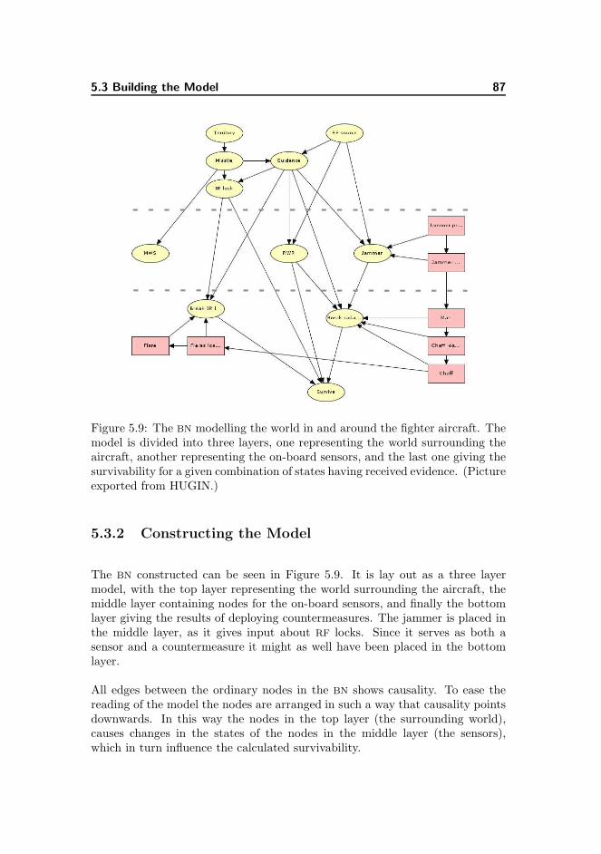
5.3 Building the Model 87
Figure 5.9: The BN modelling the world in and around the fighter aircraft. Themodel is divided into three layers, one representing the world surrounding theaircraft, another representing the on-board sensors, and the last one giving thesurvivability for a given combination of states having received evidence. (Pictureexported from HUGIN.)
5.3.2 Constructing the Model
The BN constructed can be seen in Figure 5.9. It is lay out as a three layermodel, with the top layer representing the world surrounding the aircraft, themiddle layer containing nodes for the on-board sensors, and finally the bottomlayer giving the results of deploying countermeasures. The jammer is placed inthe middle layer, as it gives input about RF locks. Since it serves as both asensor and a countermeasure it might as well have been placed in the bottomlayer.
All edges between the ordinary nodes in the BN shows causality. To ease thereading of the model the nodes are arranged in such a way that causality pointsdownwards. In this way the nodes in the top layer (the surrounding world),causes changes in the states of the nodes in the middle layer (the sensors),which in turn influence the calculated survivability.
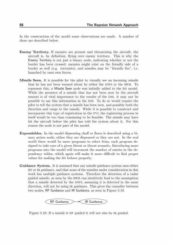
88 The Bayesian Network Approach
In the construction of the model some observations are made. A number ofthese are described below.
Enemy Territory. If enemies are present and threatening the aircraft, theaircraft is, by definition, flying over enemy territory. This is why theEnemy Territory is not just a binary node, indicating whether or not theborder has been crossed; enemies might exist on the friendly side of aborder as well (e.g. terrorists), and missiles may be ”friendly fire”, i.e.launched by ones own forces.
Missile Seen. It is possible for the pilot to visually see an incoming missilethat he has not been warned about by either the MWS or the RWR. Torepresent this, a Missile Seen node was initially added to the BN model.While the presence of a missile that has not been seen by the aircraftsensors is of vital importance to the results of the DSS, it may not bepossible to use this information in the DSS. To do so would require thepilot to tell the system that a missile has been seen, and possibly both thedirection and range to the missile. While it is possible to construct andincorporate this type of registration in the PVI, the registering process initself would be too time consuming to be feasible. The missile may havehit the aircraft before the pilot has told the system about it. For thisreason the node is not part of the model.
Expendables. In the model dispensing chaff or flares is described using a bi-nary action node; either they are dispensed or they are not. In the realworld there would be more programs to select from, each program de-signed to take care of a given threat or threat scenario. Introducing moreprograms into the model will increment the number of entries in the de-pendency tables, which again will make it more difficult to find propervalues for making the BN behave properly.
Guidance System. It is assumed that any missile guidance system uses eitherRF or IR guidance, and that none of the missiles under consideration in thiswork has multiple guidance systems. Therefore the detection of a radarguided missile, as seen by the RWR can intuitively lead to the assumptionthat a missile detected by the MWS, assuming it is detected in the samedirection, will not be using IR guidance. This gives the causality betweentwo nodes, RF Guidance and IR Guidance, as seen in Figure 5.10.
RF Guidance IR Guidance
Figure 5.10: If a missile is RF guided it will not also be IR guided.
5.3 Building the Model 89
Since RF and IR guidance are mutual exclusive there is no reason to main-tain two nodes, and the RF Guidance and IR Guidance nodes are thusmerged to a single node named Guidance.
Since different types of missiles use the same type of guidance, with dif-ferent results, the presence of an IR lock depends on both the type ofmissile and on the guidance in use. It can not depend on the missile typealone, since missiles having the same missile types may be equipped withdifferent types of guidance systems.
Decision and Utility Nodes A number of decision nodes are added to themodel. These nodes and their states can be seen in Table 5.4. Let |A|be the number of states in a decision node A. With the seven nodesin the model there are |Jammer Present| · |Jammer Mode| · |Manoeuvre| ·|Chaff Loaded| · |Chaff| · |Flares Loaded| · |Flares| = 2 · 3 · 3 · 2 · 2 · 2 · 2 = 288combinations of states in the decision nodes.
Not all decision nodes need to be part of the decision since the pilothas no way of changing the state of these while in-flight. The decisionnodes is thus split into two sets, the preparation nodes comprising theJammer Present, Chaff Loaded, and Flares Loaded, and the action nodes :Jammer Mode, Manoeuvre, Chaff, and Flares. This now gives a total of3 · 3 · 2 · 2 = 36 combinations of states in the action nodes which shouldbe tested to find the combination yielding the highest survivability. Someof these combinations would not be feasible, and could thus be removedfrom the set of combinations to test for. For instance a combination offlares and manoeuvres does not make any sense, if Flares Loaded indicatethat no flares are available.
Decision node: States:Jammer Present Yes, NoJammer Mode Off, Rx, AutoManoeuvre None, Left, RightChaff Loaded Yes, NoChaff No, DispenseFlares Loaded Yes, NoFlares No, Dispense
Table 5.4: The decision nodes and their states.
As can be seen in Figure 5.9 the action nodes are interconnected. InSection 5.2.6 it is stated that action nodes have no dependency tables,and the edges between action nodes does not constitute a parent-childrelation per se. Instead they are needed for the propagation algorithmused by HUGIN. The direction of the arrows between the action nodes isof no influence to the calculated survivability.
90 The Bayesian Network Approach
As described in Section 5.2.6 the introduction of a utility scale for themodel is not straightforward. At first the number of remaining expend-ables was introduced as a utility scale and utility nodes were connectedto the Flare and Chaff nodes. This is skipped since flares and chaff aretwo very different types of expendables, and having a number of flares leftwill not increase the survivability when a RF based threat occurs. Sec-ond, optimizing the amount of inventory would only result in using lessexpendable, not in increasing the survivability at all. For these reasons noutility nodes are used in the final model.
5.4 Populating Dependency Tables
The work with constructing a BN can be divided into two parts: the constructionof the qualitative structure of the net, where all nodes and dependencies betweennodes are established, and the quantitative population of the dependency tables.Different approaches to ease the latter part of the process have been tried. In[17] the relations between nodes are described using Prolog-like Horn clausesand by parting the network into self-contained objects, and in [24] the degreesof certainty in relations are described using simple sentences in semi-naturalEnglish. While these approaches have some advantages in the initial populationof dependency tables, they do not appeal to the strength of using a precision toolas BN. The HUGIN tool offers different techniques for describing the probabilitydistributions using e.g. discrete distributions or arithmetic functions.
5.4.1 Multi-dependency Tables
In this work a simple model describing the domain is developed. This modelcontains the nodes deemed necessary for decision support for fighter pilots, andeach of the nodes has a very limited number of states. In simple tests thesimple model works as expected, but it does not handle the complexity of e.g.several different missile types and guidance systems. Therefore the model isexpanded by adding more states to some of the nodes. Going from e.g. twovalues for the Missile node (Present/Not present) to 12 values (Not present and11 different missile types) gives not only six times as many entries in the Missilenode dependency table, but also in the tables of all nodes dependent on theMissile node.
This section describes a semi-automatic procedure for producing multi-dependencytables, i.e. tables giving the dependency of multiple parents. For nodes hav-
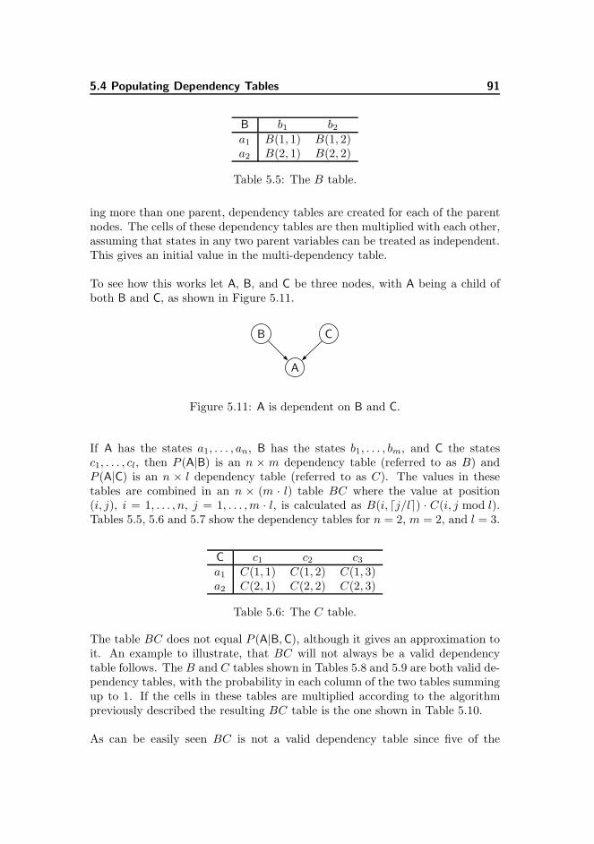
5.4 Populating Dependency Tables 91
B b1 b2
a1 B(1, 1) B(1, 2)a2 B(2, 1) B(2, 2)
Table 5.5: The B table.
ing more than one parent, dependency tables are created for each of the parentnodes. The cells of these dependency tables are then multiplied with each other,assuming that states in any two parent variables can be treated as independent.This gives an initial value in the multi-dependency table.
To see how this works let A, B, and C be three nodes, with A being a child ofboth B and C, as shown in Figure 5.11.
B C
A
Figure 5.11: A is dependent on B and C.
If A has the states a1, . . . , an, B has the states b1, . . . , bm, and C the statesc1, . . . , cl, then P (A|B) is an n × m dependency table (referred to as B) andP (A|C) is an n × l dependency table (referred to as C). The values in thesetables are combined in an n × (m · l) table BC where the value at position(i, j), i = 1, . . . , n, j = 1, . . . , m · l, is calculated as B(i, dj/le) · C(i, j mod l).Tables 5.5, 5.6 and 5.7 show the dependency tables for n = 2, m = 2, and l = 3.
C c1 c2 c3
a1 C(1, 1) C(1, 2) C(1, 3)a2 C(2, 1) C(2, 2) C(2, 3)
Table 5.6: The C table.
The table BC does not equal P (A|B, C), although it gives an approximation toit. An example to illustrate, that BC will not always be a valid dependencytable follows. The B and C tables shown in Tables 5.8 and 5.9 are both valid de-pendency tables, with the probability in each column of the two tables summingup to 1. If the cells in these tables are multiplied according to the algorithmpreviously described the resulting BC table is the one shown in Table 5.10.
As can be easily seen BC is not a valid dependency table since five of the
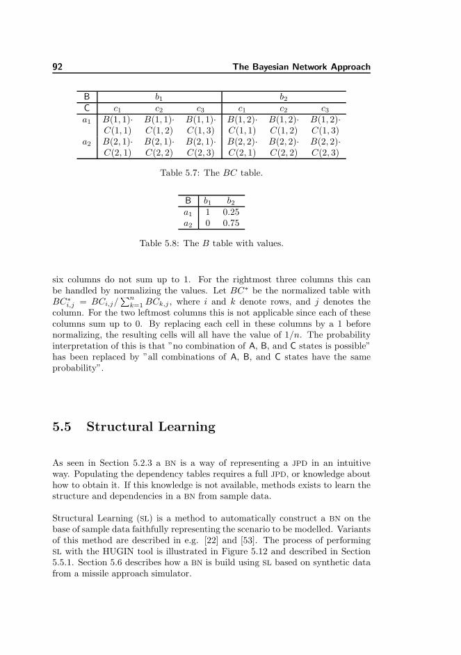
92 The Bayesian Network Approach
B b1 b2
C c1 c2 c3 c1 c2 c3
a1 B(1, 1)· B(1, 1)· B(1, 1)· B(1, 2)· B(1, 2)· B(1, 2)·C(1, 1) C(1, 2) C(1, 3) C(1, 1) C(1, 2) C(1, 3)
a2 B(2, 1)· B(2, 1)· B(2, 1)· B(2, 2)· B(2, 2)· B(2, 2)·C(2, 1) C(2, 2) C(2, 3) C(2, 1) C(2, 2) C(2, 3)
Table 5.7: The BC table.
B b1 b2
a1 1 0.25a2 0 0.75
Table 5.8: The B table with values.
six columns do not sum up to 1. For the rightmost three columns this canbe handled by normalizing the values. Let BC∗ be the normalized table withBC∗
i,j = BCi,j/Pn
k=1 BCk,j , where i and k denote rows, and j denotes thecolumn. For the two leftmost columns this is not applicable since each of thesecolumns sum up to 0. By replacing each cell in these columns by a 1 beforenormalizing, the resulting cells will all have the value of 1/n. The probabilityinterpretation of this is that ”no combination of A, B, and C states is possible”has been replaced by ”all combinations of A, B, and C states have the sameprobability”.
5.5 Structural Learning
As seen in Section 5.2.3 a BN is a way of representing a JPD in an intuitiveway. Populating the dependency tables requires a full JPD, or knowledge abouthow to obtain it. If this knowledge is not available, methods exists to learn thestructure and dependencies in a BN from sample data.
Structural Learning (SL) is a method to automatically construct a BN on thebase of sample data faithfully representing the scenario to be modelled. Variantsof this method are described in e.g. [22] and [53]. The process of performingSL with the HUGIN tool is illustrated in Figure 5.12 and described in Section5.5.1. Section 5.6 describes how a BN is build using SL based on synthetic datafrom a missile approach simulator.
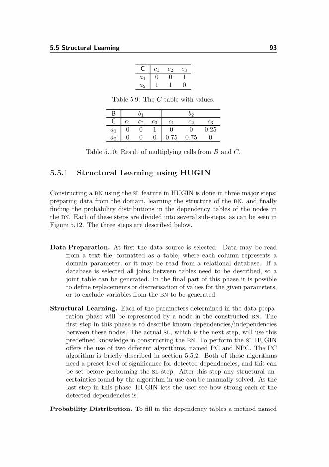
5.5 Structural Learning 93
C c1 c2 c3
a1 0 0 1a2 1 1 0
Table 5.9: The C table with values.
B b1 b2
C c1 c2 c3 c1 c2 c3
a1 0 0 1 0 0 0.25a2 0 0 0 0.75 0.75 0
Table 5.10: Result of multiplying cells from B and C.
5.5.1 Structural Learning using HUGIN
Constructing a BN using the SL feature in HUGIN is done in three major steps:preparing data from the domain, learning the structure of the BN, and finallyfinding the probability distributions in the dependency tables of the nodes inthe BN. Each of these steps are divided into several sub-steps, as can be seen inFigure 5.12. The three steps are described below.
Data Preparation. At first the data source is selected. Data may be readfrom a text file, formatted as a table, where each column represents adomain parameter, or it may be read from a relational database. If adatabase is selected all joins between tables need to be described, so ajoint table can be generated. In the final part of this phase it is possibleto define replacements or discretisation of values for the given parameters,or to exclude variables from the BN to be generated.
Structural Learning. Each of the parameters determined in the data prepa-ration phase will be represented by a node in the constructed BN. Thefirst step in this phase is to describe known dependencies/independenciesbetween these nodes. The actual SL, which is the next step, will use thispredefined knowledge in constructing the BN. To perform the SL HUGINoffers the use of two different algorithms, named PC and NPC. The PCalgorithm is briefly described in section 5.5.2. Both of these algorithmsneed a preset level of significance for detected dependencies, and this canbe set before performing the SL step. After this step any structural un-certainties found by the algorithm in use can be manually solved. As thelast step in this phase, HUGIN lets the user see how strong each of thedetected dependencies is.
Probability Distribution. To fill in the dependency tables a method named
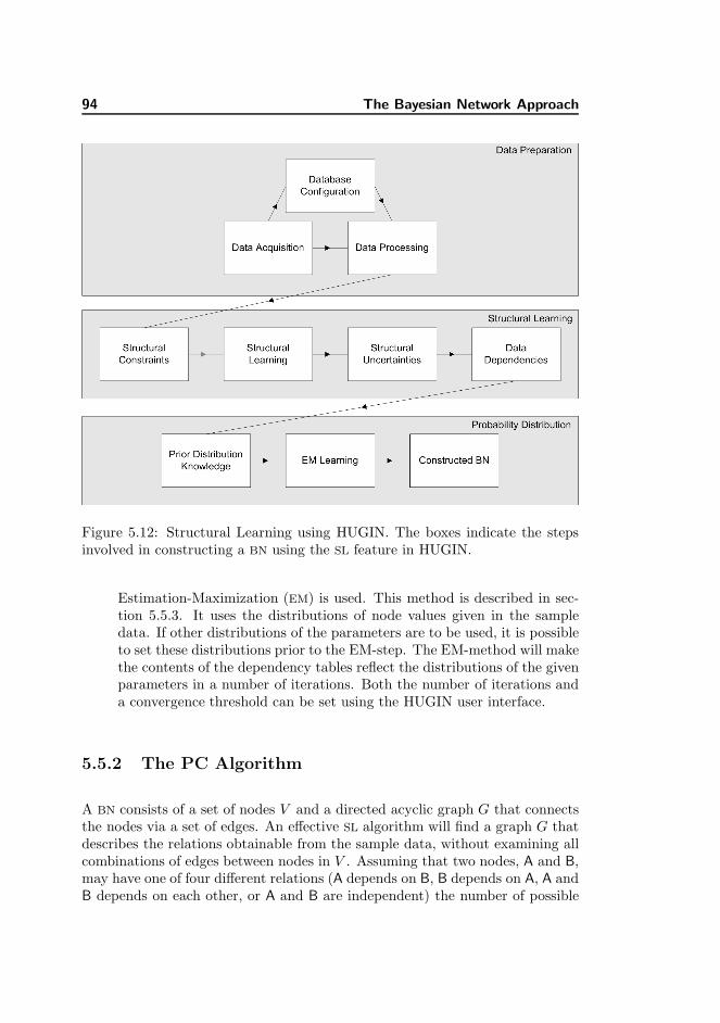
94 The Bayesian Network Approach
Figure 5.12: Structural Learning using HUGIN. The boxes indicate the stepsinvolved in constructing a BN using the SL feature in HUGIN.
Estimation-Maximization (EM) is used. This method is described in sec-tion 5.5.3. It uses the distributions of node values given in the sampledata. If other distributions of the parameters are to be used, it is possibleto set these distributions prior to the EM-step. The EM-method will makethe contents of the dependency tables reflect the distributions of the givenparameters in a number of iterations. Both the number of iterations anda convergence threshold can be set using the HUGIN user interface.
5.5.2 The PC Algorithm
A BN consists of a set of nodes V and a directed acyclic graph G that connectsthe nodes via a set of edges. An effective SL algorithm will find a graph G thatdescribes the relations obtainable from the sample data, without examining allcombinations of edges between nodes in V . Assuming that two nodes, A and B,may have one of four different relations (A depends on B, B depends on A, A andB depends on each other, or A and B are independent) the number of possible
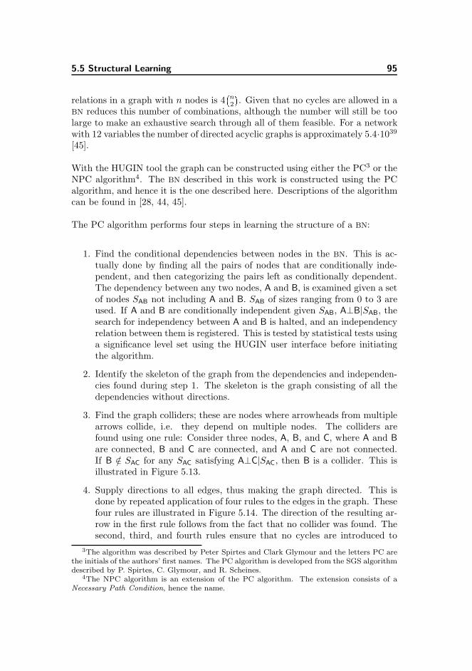
5.5 Structural Learning 95
relations in a graph with n nodes is 4�n2
�. Given that no cycles are allowed in a
BN reduces this number of combinations, although the number will still be toolarge to make an exhaustive search through all of them feasible. For a networkwith 12 variables the number of directed acyclic graphs is approximately 5.4·1039
[45].
With the HUGIN tool the graph can be constructed using either the PC3 or theNPC algorithm4. The BN described in this work is constructed using the PCalgorithm, and hence it is the one described here. Descriptions of the algorithmcan be found in [28, 44, 45].
The PC algorithm performs four steps in learning the structure of a BN:
1. Find the conditional dependencies between nodes in the BN. This is ac-tually done by finding all the pairs of nodes that are conditionally inde-pendent, and then categorizing the pairs left as conditionally dependent.The dependency between any two nodes, A and B, is examined given a setof nodes SAB not including A and B. SAB of sizes ranging from 0 to 3 areused. If A and B are conditionally independent given SAB, A⊥B|SAB, thesearch for independency between A and B is halted, and an independencyrelation between them is registered. This is tested by statistical tests usinga significance level set using the HUGIN user interface before initiatingthe algorithm.
2. Identify the skeleton of the graph from the dependencies and independen-cies found during step 1. The skeleton is the graph consisting of all thedependencies without directions.
3. Find the graph colliders; these are nodes where arrowheads from multiplearrows collide, i.e. they depend on multiple nodes. The colliders arefound using one rule: Consider three nodes, A, B, and C, where A and Bare connected, B and C are connected, and A and C are not connected.If B /∈ SAC for any SAC satisfying A⊥C|SAC, then B is a collider. This isillustrated in Figure 5.13.
4. Supply directions to all edges, thus making the graph directed. This isdone by repeated application of four rules to the edges in the graph. Thesefour rules are illustrated in Figure 5.14. The direction of the resulting ar-row in the first rule follows from the fact that no collider was found. Thesecond, third, and fourth rules ensure that no cycles are introduced to
3The algorithm was described by Peter Spirtes and Clark Glymour and the letters PC arethe initials of the authors’ first names. The PC algorithm is developed from the SGS algorithmdescribed by P. Spirtes, C. Glymour, and R. Scheines.
4The NPC algorithm is an extension of the PC algorithm. The extension consists of aNecessary Path Condition, hence the name.
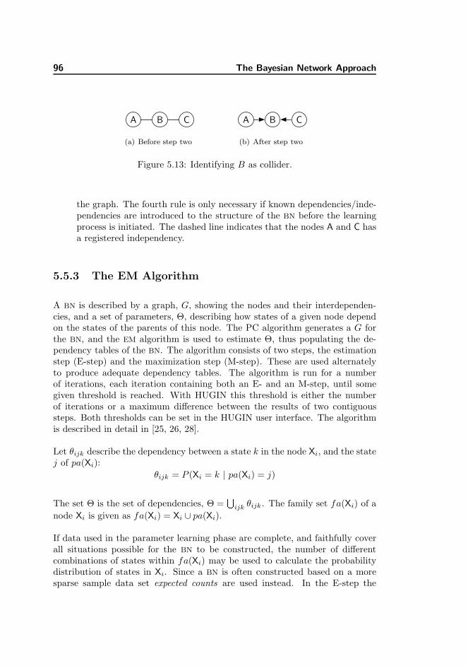
96 The Bayesian Network Approach
A B C
(a) Before step two
A B C
(b) After step two
Figure 5.13: Identifying B as collider.
the graph. The fourth rule is only necessary if known dependencies/inde-pendencies are introduced to the structure of the BN before the learningprocess is initiated. The dashed line indicates that the nodes A and C hasa registered independency.
5.5.3 The EM Algorithm
A BN is described by a graph, G, showing the nodes and their interdependen-cies, and a set of parameters, Θ, describing how states of a given node dependon the states of the parents of this node. The PC algorithm generates a G forthe BN, and the EM algorithm is used to estimate Θ, thus populating the de-pendency tables of the BN. The algorithm consists of two steps, the estimationstep (E-step) and the maximization step (M-step). These are used alternatelyto produce adequate dependency tables. The algorithm is run for a numberof iterations, each iteration containing both an E- and an M-step, until somegiven threshold is reached. With HUGIN this threshold is either the numberof iterations or a maximum difference between the results of two contiguoussteps. Both thresholds can be set in the HUGIN user interface. The algorithmis described in detail in [25, 26, 28].
Let θijk describe the dependency between a state k in the node Xi, and the statej of pa(Xi):
θijk = P (Xi = k | pa(Xi) = j)
The set Θ is the set of dependencies, Θ =S
ijk θijk. The family set fa(Xi) of a
node Xi is given as fa(Xi) = Xi ∪ pa(Xi).
If data used in the parameter learning phase are complete, and faithfully coverall situations possible for the BN to be constructed, the number of differentcombinations of states within fa(Xi) may be used to calculate the probabilitydistribution of states in Xi. Since a BN is often constructed based on a moresparse sample data set expected counts are used instead. In the E-step the
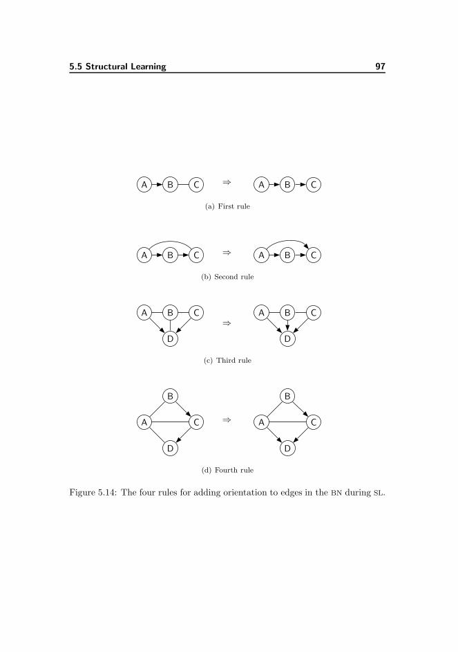
5.5 Structural Learning 97
A B C ⇒ A B C
(a) First rule
A B C ⇒ A B C
(b) Second rule
A B C
D
⇒A B C
D
(c) Third rule
A
B
C
D
⇒ A
B
C
D
(d) Fourth rule
Figure 5.14: The four rules for adding orientation to edges in the BN during SL.
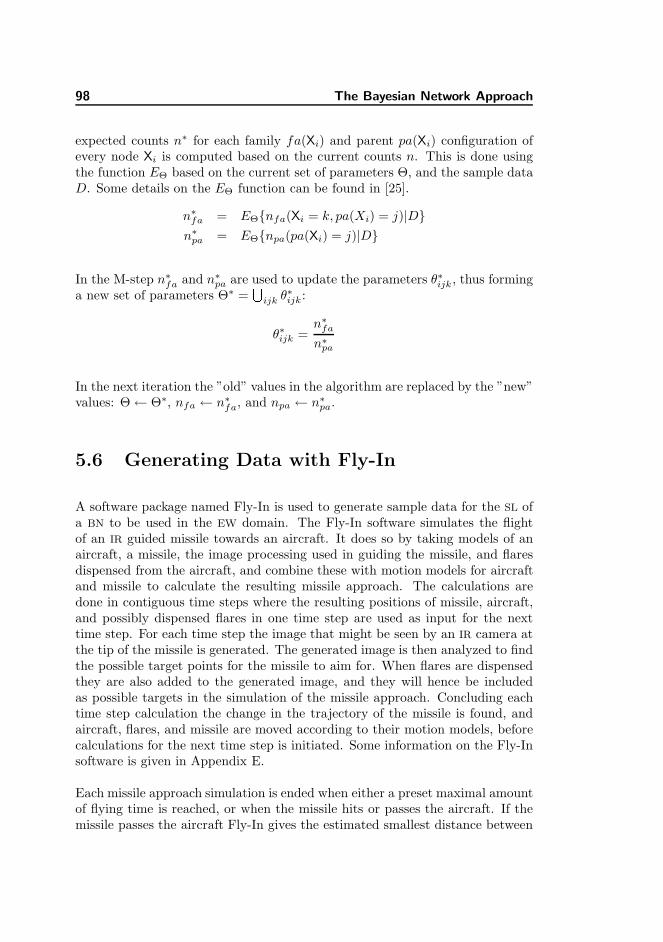
98 The Bayesian Network Approach
expected counts n∗ for each family fa(Xi) and parent pa(Xi) configuration ofevery node Xi is computed based on the current counts n. This is done usingthe function EΘ based on the current set of parameters Θ, and the sample dataD. Some details on the EΘ function can be found in [25].
n∗fa = EΘ{nfa(Xi = k, pa(Xi) = j)|D}
n∗pa = EΘ{npa(pa(Xi) = j)|D}
In the M-step n∗fa and n∗
pa are used to update the parameters θ∗ijk, thus forminga new set of parameters Θ∗ =
Sijk θ∗ijk:
θ∗ijk =n∗
fa
n∗pa
In the next iteration the ”old” values in the algorithm are replaced by the ”new”values: Θ← Θ∗, nfa ← n∗
fa, and npa ← n∗pa.
5.6 Generating Data with Fly-In
A software package named Fly-In is used to generate sample data for the SL ofa BN to be used in the EW domain. The Fly-In software simulates the flightof an IR guided missile towards an aircraft. It does so by taking models of anaircraft, a missile, the image processing used in guiding the missile, and flaresdispensed from the aircraft, and combine these with motion models for aircraftand missile to calculate the resulting missile approach. The calculations aredone in contiguous time steps where the resulting positions of missile, aircraft,and possibly dispensed flares in one time step are used as input for the nexttime step. For each time step the image that might be seen by an IR camera atthe tip of the missile is generated. The generated image is then analyzed to findthe possible target points for the missile to aim for. When flares are dispensedthey are also added to the generated image, and they will hence be includedas possible targets in the simulation of the missile approach. Concluding eachtime step calculation the change in the trajectory of the missile is found, andaircraft, flares, and missile are moved according to their motion models, beforecalculations for the next time step is initiated. Some information on the Fly-Insoftware is given in Appendix E.
Each missile approach simulation is ended when either a preset maximal amountof flying time is reached, or when the missile hits or passes the aircraft. If themissile passes the aircraft Fly-In gives the estimated smallest distance between
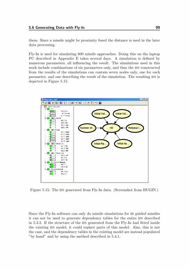
5.6 Generating Data with Fly-In 99
them. Since a missile might be proximity fused the distance is used in the laterdata processing.
Fly-In is used for simulating 600 missile approaches. Doing this on the laptopPC described in Appendix E takes several days. A simulation is defined bynumerous parameters, all influencing the result. The simulations used in thiswork include combinations of six parameters only, and thus the BN constructedfrom the results of the simulations can contain seven nodes only, one for eachparameter, and one describing the result of the simulation. The resulting BN isdepicted in Figure 5.15.
Figure 5.15: The BN generated from Fly-In data. (Screenshot from HUGIN.)
Since the Fly-In software can only do missile simulations for IR guided missilesit can not be used to generate dependency tables for the entire BN describedin 5.3.2. If the structure of the BN generated from the Fly-In had fitted insidethe existing BN model, it could replace parts of this model. Alas, this is notthe case, and the dependency tables in the existing model are instead populated”by hand” and by using the method described in 5.4.1.
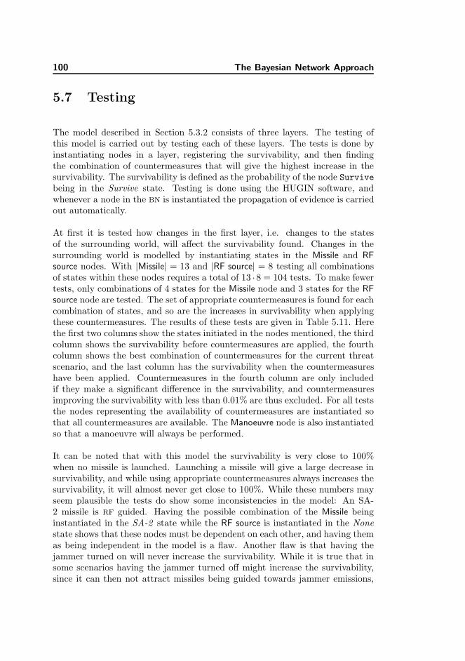
100 The Bayesian Network Approach
5.7 Testing
The model described in Section 5.3.2 consists of three layers. The testing ofthis model is carried out by testing each of these layers. The tests is done byinstantiating nodes in a layer, registering the survivability, and then findingthe combination of countermeasures that will give the highest increase in thesurvivability. The survivability is defined as the probability of the node Survivebeing in the Survive state. Testing is done using the HUGIN software, andwhenever a node in the BN is instantiated the propagation of evidence is carriedout automatically.
At first it is tested how changes in the first layer, i.e. changes to the statesof the surrounding world, will affect the survivability found. Changes in thesurrounding world is modelled by instantiating states in the Missile and RFsource nodes. With |Missile| = 13 and |RF source| = 8 testing all combinationsof states within these nodes requires a total of 13 · 8 = 104 tests. To make fewertests, only combinations of 4 states for the Missile node and 3 states for the RFsource node are tested. The set of appropriate countermeasures is found for eachcombination of states, and so are the increases in survivability when applyingthese countermeasures. The results of these tests are given in Table 5.11. Herethe first two columns show the states initiated in the nodes mentioned, the thirdcolumn shows the survivability before countermeasures are applied, the fourthcolumn shows the best combination of countermeasures for the current threatscenario, and the last column has the survivability when the countermeasureshave been applied. Countermeasures in the fourth column are only includedif they make a significant difference in the survivability, and countermeasuresimproving the survivability with less than 0.01% are thus excluded. For all teststhe nodes representing the availability of countermeasures are instantiated sothat all countermeasures are available. The Manoeuvre node is also instantiatedso that a manoeuvre will always be performed.
It can be noted that with this model the survivability is very close to 100%when no missile is launched. Launching a missile will give a large decrease insurvivability, and while using appropriate countermeasures always increases thesurvivability, it will almost never get close to 100%. While these numbers mayseem plausible the tests do show some inconsistencies in the model: An SA-2 missile is RF guided. Having the possible combination of the Missile beinginstantiated in the SA-2 state while the RF source is instantiated in the Nonestate shows that these nodes must be dependent on each other, and having themas being independent in the model is a flaw. Another flaw is that having thejammer turned on will never increase the survivability. While it is true that insome scenarios having the jammer turned off might increase the survivability,since it can then not attract missiles being guided towards jammer emissions,
5.7 Testing 101
Missile: RF source: PS before: Countermeasures: PS after:No missile None 100,00% None 100,00%No missile X band 99,87% Flares 99,99%No missile L band 99,90% Flares 99,99%SA-2 None 40,88% Chaff 43,18%SA-2 X band 64,97% Chaff, no jammer 67,73%SA-2 L band 64,80% Chaff, no jammer 67,13%Stinger Basic None 58,15% Flares 86,98%Stinger Basic X band 59,37% Flares 91,09%Stinger Basic L band 57,67% Chaff, flares 87,10%HAWK None 57,42% Chaff 59,10%HAWK X band 65,96% Chaff, no jammer 68,67%HAWK L band 68,63% Chaff, no jammer 70,75%
Table 5.11: Testing the first layer of the BN model. Changing the surroundings(the nodes Missile and RF source) influence the survivability (PS before). Whencountermeasures are applied the survivability changes (PS after).
having it turned off will in general not have this effect. When RF radiation ispresent, and no missile has been launched, the use of a jammer will generallyincrease the survivability. This is not shown by the tests.
In testing the second layer of the model the influence on the survivability byinput from on-board systems is evaluated. This is done with combinations of thestates of the MWS, RWR, and Jammer nodes. Of the |MWS| · |RWR| · |Jammer| =2 · 4 · 5 = 40 combinations of states in these nodes 2 · 3 · 2 = 12 are selected. Thecircumstances with these tests are the same as for testing the first layer. Theresults are shown in Table 5.12.
From these results it can be seen that having the RWR registering a radar lockwill give a remarkably low survivability. Even if proper countermeasures areapplied the survivability will not increase very much. The results also revealother inexpediencies with the survivabilities related to RWR warnings: If theRWR detects a RF source, that is likely to be a threat, the survivability is higherthan if the RWR detects no RF source. When prior to using countermeasuresthe survivability is at 100% no countermeasures can increase the survivability.For all other test cases the use of proper countermeasures will increase thesurvivability, although the size of this increase may be questionable.
Testing the first and the second layer shows the influence on changes in thesurvivability. Since survivability is the probability of the third layer node Survivebeing in the state Survive, tests of the third layer can show how changes to thisnode influence the probability distribution in the rest of the BN. To do this
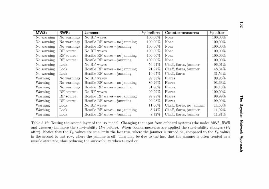
102
The
Bayesia
nN
etw
ork
Appro
ach
MWS: RWR: Jammer: PS before: Countermeasures: PS after:No warning No warnings No RF waves 100,00% None 100,00%No warning No warnings Hostile RF waves - no jamming 100,00% None 100,00%No warning No warnings Hostile RF waves - jamming 100,00% None 100,00%No warning RF source No RF waves 100,00% None 100,00%No warning RF source Hostile RF waves - no jamming 100,00% None 100,00%No warning RF source Hostile RF waves - jamming 100,00% None 100,00%No warning Lock No RF waves 56,94% Chaff, flares, jammer 96,01%No warning Lock Hostile RF waves - no jamming 21,97% Chaff, flares, jammer 48,34%No warning Lock Hostile RF waves - jamming 19,97% Chaff, flares 31,54%Warning No warnings No RF waves 99,88% Flares 99,96%Warning No warnings Hostile RF waves - no jamming 80,26% Flares 93,63%Warning No warnings Hostile RF waves - jamming 81,80% Flares 94,13%Warning RF source No RF waves 99,99% Flares 100,00%Warning RF source Hostile RF waves - no jamming 99,98% Flares 99,99%Warning RF source Hostile RF waves - jamming 99,98% Flares 99,99%Warning Lock No RF waves 11,00% Chaff, flares, no jammer 14,50%Warning Lock Hostile RF waves - no jamming 8,74% Chaff, flares, jammer 11,92%Warning Lock Hostile RF waves - jamming 8,72% Chaff, flares, jammer 11,81%
Table 5.12: Testing the second layer of the BN model. Changing the input from onboard systems (the nodes MWS, RWRand Jammer) influence the survivability (PS before). When countermeasures are applied the survivability changes (PS
after). Notice that the PS values are smaller in the last row, where the jammer is turned on, compared to the PS valuesin the second to last row, where the jammer is off. This may be due to the fact that the jammer is often treated as amissile attractor, thus reducing the survivability when turned on.
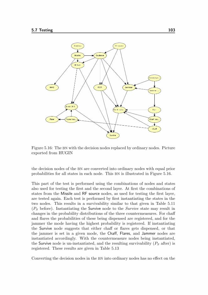
5.7 Testing 103
Figure 5.16: The BN with the decision nodes replaced by ordinary nodes. Pictureexported from HUGIN
the decision nodes of the BN are converted into ordinary nodes with equal priorprobabilities for all states in each node. This BN is illustrated in Figure 5.16.
This part of the test is performed using the combinations of nodes and statesalso used for testing the first and the second layer. At first the combinations ofstates from the Missile and RF source nodes, as used for testing the first layer,are tested again. Each test is performed by first instantiating the states in thetwo nodes. This results in a survivability similar to that given in Table 5.11(PS before). Instantiating the Survive node to the Survive state may result inchanges in the probability distributions of the three countermeasures. For chaffand flares the probabilities of these being dispensed are registered, and for thejammer the mode having the highest probability is registered. If instantiatingthe Survive node suggests that either chaff or flares gets dispensed, or thatthe jammer is set in a given mode, the Chaff, Flares, and Jammer nodes areinstantiated accordingly. With the countermeasure nodes being instantiated,the Survive node is un-instantiated, and the resulting survivability (PS after) isregistered. These results are given in Table 5.13
Converting the decision nodes in the BN into ordinary nodes has no effect on the
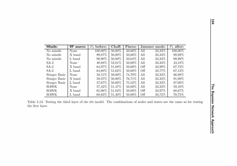
104
The
Bayesia
nN
etw
ork
Appro
ach
Missile: RF source: PS before: Chaff: Flares: Jammer mode: PS after:No missile None 100,00% 50,00% 50,00% All 33,33% 100,00%No missile X band 99,87% 50,00% 50,06% All 33,33% 99,99%No missile L band 99,90% 50,00% 50,04% All 33,33% 99,99%SA-2 None 40,88% 52,81% 50,00% All 33,33% 43,18%SA-2 X band 64,97% 51,88% 50,00% Off 33,99% 67,73%SA-2 L band 64,80% 51,62% 50,00% Off 33,77% 67,13%Stinger Basic None 58,15% 50,00% 74,79% All 33,33% 86,98%Stinger Basic X band 59,37% 50,00% 76,71% All 33,33% 91,09%Stinger Basic L band 57,67% 50,00% 75,52% All 33,33% 87,09%HAWK None 57,42% 51,47% 50,00% All 33,33% 59,10%HAWK X band 65,96% 51,82% 50,00% Off 33,97% 68,67%HAWK L band 68,63% 51,40% 50,00% Off 33,72% 70,75%
Table 5.13: Testing the third layer of the BN model. The combinations of nodes and states are the same as for testingthe first layer.
5.8 Discussion 105
survivabilities found. This can be seen by comparing the values in the third (PS
before) and the last column (PS after) with the similar columns in Table 5.11.The major difference between working with the BN containing decision nodesand the BN without decision nodes is that with the latter a good combinationof countermeasures is found by instantiating the Survive node only.
In the final part of the BN test the combinations of states in the MWS, RWR,and Jammer nodes, as used for testing the second layer, is tested again. Table5.14 holds the results of these tests.
Comparing the PS values in Table 5.12 and Table 5.14 shows differences betweenthe survivabilities found. The PS values found before countermeasures are ap-plied are identical, but after applying countermeasures they tend to be smallerin Table 5.14. The reason for this is that instantiating the Survive node does notguarantee that the best combination of countermeasures is found, and instanti-ating the countermeasures in the BN without action nodes, according to the setof countermeasures given in Table 5.12, will result in the same survivabilities asgiven here.
5.8 Discussion
It seems that a BN can be useful in modelling a domain where not all knowledgeis categorical. In a DSS where decisions are based on uncertain observationsthe uncertainties can themselves, if they can be estimated, become part of thedecision base. For the threat situation in a fighter aircraft the use of a BN seemsadequate since decisions here will often be based on imperfect data from sensorson-board the aircraft. A reason for using a BN is that it is relatively easy to builda model for the threat response situation, and that this model can be built toreflect the uncertainties related to sensor output. The down side of using a BN
for modelling the threat situation is that it requires a vast amount of knowledgeto be represented in dependency tables in the BN.
Section 5.4.1 describes a semi-automatic method for populating dependency ta-bles for nodes which depends on multiple parents. The method is not applicablefor populating single parent dependency tables, and to be applicable for mul-tiple parent dependency tables it needs a dependency table set up for each ofthe parents. The labour of finding proper values to populate these tables is notdiminished by this method, and the resulting multi-dependency tables are notvalid if the parents are interdependent.
Using the SL method described in Section 5.5 the dependency tables of the BN are
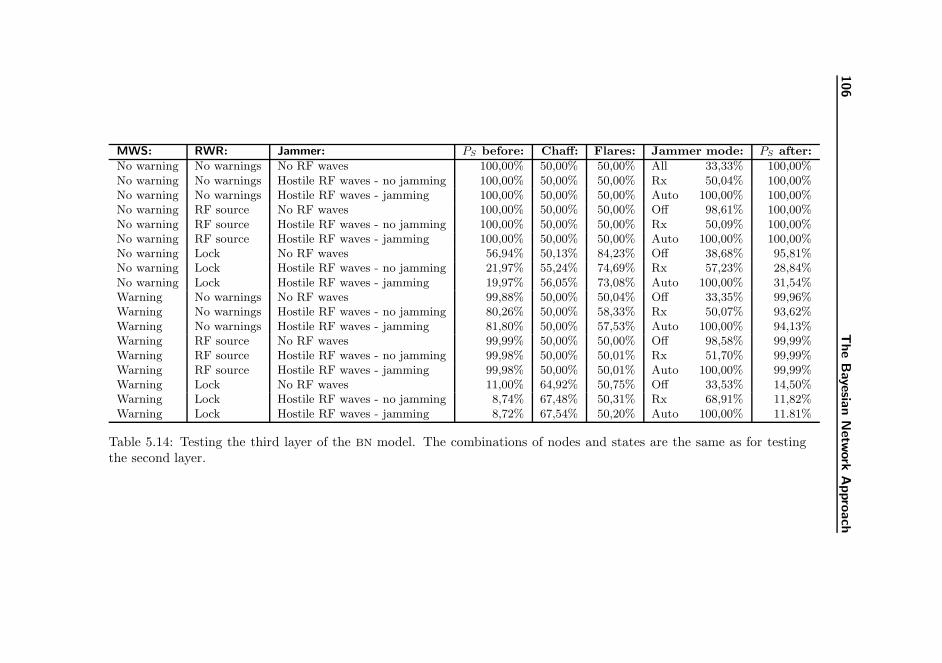
106
The
Bayesia
nN
etw
ork
Appro
ach
MWS: RWR: Jammer: PS before: Chaff: Flares: Jammer mode: PS after:
No warning No warnings No RF waves 100,00% 50,00% 50,00% All 33,33% 100,00%No warning No warnings Hostile RF waves - no jamming 100,00% 50,00% 50,00% Rx 50,04% 100,00%No warning No warnings Hostile RF waves - jamming 100,00% 50,00% 50,00% Auto 100,00% 100,00%No warning RF source No RF waves 100,00% 50,00% 50,00% Off 98,61% 100,00%No warning RF source Hostile RF waves - no jamming 100,00% 50,00% 50,00% Rx 50,09% 100,00%No warning RF source Hostile RF waves - jamming 100,00% 50,00% 50,00% Auto 100,00% 100,00%No warning Lock No RF waves 56,94% 50,13% 84,23% Off 38,68% 95,81%No warning Lock Hostile RF waves - no jamming 21,97% 55,24% 74,69% Rx 57,23% 28,84%No warning Lock Hostile RF waves - jamming 19,97% 56,05% 73,08% Auto 100,00% 31,54%Warning No warnings No RF waves 99,88% 50,00% 50,04% Off 33,35% 99,96%Warning No warnings Hostile RF waves - no jamming 80,26% 50,00% 58,33% Rx 50,07% 93,62%Warning No warnings Hostile RF waves - jamming 81,80% 50,00% 57,53% Auto 100,00% 94,13%Warning RF source No RF waves 99,99% 50,00% 50,00% Off 98,58% 99,99%Warning RF source Hostile RF waves - no jamming 99,98% 50,00% 50,01% Rx 51,70% 99,99%Warning RF source Hostile RF waves - jamming 99,98% 50,00% 50,01% Auto 100,00% 99,99%Warning Lock No RF waves 11,00% 64,92% 50,75% Off 33,53% 14,50%Warning Lock Hostile RF waves - no jamming 8,74% 67,48% 50,31% Rx 68,91% 11,82%Warning Lock Hostile RF waves - jamming 8,72% 67,54% 50,20% Auto 100,00% 11.81%
Table 5.14: Testing the third layer of the BN model. The combinations of nodes and states are the same as for testingthe second layer.
5.9 Conclusion 107
populated regardless of the number of parents for each node. The drawback ofusing this method is that it requires a dataset faithfully representing the domainto model. If this dataset is available, either from real-world observations or fromsynthetic data, e.g. based on simulations, the SL feature will produce a usableBN or it will populate the dependency tables in an existing BN structure.
With both these methods the major part of the work is related to the gatheringof detailed data describing the domain. A large part of the knowledge necessaryfor populating these dependency tables does either not exist or it is restrictedand thus unavailable. Therefore constructing a BN to represent the relations inthe EW domain for fighter pilots may become difficult or even impossible.
It is still possible to construct a simpler model that does not show the exactrelations from a real world scenario. While this model will have flaws in somescenarios it may still be adequate for decision support in most situations.
In this work the HUGIN tool is used for both constructing the BN and forupdating it during tests whenever nodes receive evidence. This is done usinga graphical user interface, and while this seems fast it is difficult to evaluatewhether the real-time requirement described in Section 3.3 is met. As describedin Section 5.7 the model developed in this work has a small number of combina-tions of actions, and finding the combination yielding the best survivability canbe done relatively fast. It is therefore assessed that the real-time requirementcan be fulfilled using a BN for decision support if proprietary software for han-dling the necessary BN updates was written, so that time spent on e.g. updatinga graphical user interface can be avoided.
5.9 Conclusion
This works has shown that it is possible to construct a simple BN to model thethreat scenario and possible outcome of different combinations of countermea-sures and manoeuvres for a fighter aircraft. The easy part of this is to definerelationships between variables/nodes in the domain, while the hard part is toqualify these relationships by populating the dependency tables.
With a lack of real-world data the BN constructed is made on simple assumptionsand it suffers from obvious errors, e.g. that the probabilities for survival willalmost always be smaller than in a real-world scenario. Despite of this the testsshow that most times the proper combination of countermeasures is found usingthe BN. It is not evident that this BN can be used in a DSS for fighter pilots,since the model constructed in this work is based on imaginary values only. In

108 The Bayesian Network Approach
constructing a model for real-world use more elaborate data should be used.
It seems that using a BN for decision support in fighter aircraft can be considereda viable approach only if necessary data describing the domain are available. Ifthis is the case it is estimated that a proper BN can be constructed to be usedfor this purpose.
Chapter 6
The Mathematical Modelling
Approach
When a threat occurs for which expendable countermeasures are an appropriateresponse these countermeasure may be applied to improve the survivability ofthe aircraft. As an aircraft is equipped with a limited number of expendablesonly, releasing all expendables at once may later bring the aircraft in a situationwhere expendables are needed without being available. Knowledge about threatsthat may engage the aircraft during a mission can help find the best overall useof the expendables. In situations where non-expandable countermeasures mayoffer nearly as good a protection as expendables, choosing the first over thelatter may increase the survivability of the aircraft for the whole mission.
This chapter introduces a survivability measure. Determining which combina-tion of countermeasures that will give the aircraft the highest probability ofsurviving a mission will be a matter of optimising this survivability measure.The influence on this measure by a set of countermeasures is described. Amathematical model to describe the countermeasures, temporal aspects abouttheir use, and their contribution to the survivability is developed. Optimisingthe survivability for flights in a number of scenarios given is done by solving theproblem described by the mathematical model for these flights.
110 The Mathematical Modelling Approach
6.1 Motivation
With the Prolog program (Chapter 4) or the BN (Chapter 5) the best coun-termeasure response can be found to the threat scenario at any given time. Infinding these responses the countermeasures are assumed instantly active andthe need for countermeasures at a later state in the mission is not considered.Introducing these aspects to the problem of finding the highest survivability forthe aircraft may require the time frame of a mission to be discretised into a fi-nite number of time steps. Finding the highest survivability for the pilot is thenaccomplished by finding the optimal combination of survivabilities for each ofthese time steps. To measure the survivability in each time step a survivabilitymeasure can be introduced. This measure must be based on both the currentthreat scenario and the countermeasures applied.
The problem of finding appropriate use of countermeasures during a missionwill also include the amount of expendable countermeasures available and therestrictions imposed by e.g. the time it takes for the countermeasures to becomeactive. For every feasible solution to this problem a survivability can be found,and the best solution will give the optimal survivability. For even very smallproblems described by few time steps only, evaluating all possible solutions tofind the best will not be feasible due to the vast amount of solutions.
It will be possible to describe the countermeasures, how they are turned on, andwhen they become active, with a mathematical model. Also their influence onthreats and the limitations set by the number of expendables available can bedescribed. Therefore it is chosen to describe the problem using a mathematicalmodel, which can then be solved to optimality.
6.2 Linear Programming
This section describes some basic theory on linear programming. Short intro-ductions to both the CPLEX solver and to the General Algebraic ModelingSystem (GAMS) are also given. Readers familiar with these subject are encour-aged to skip this section and continue with Section 6.3.
An optimisation problem is described using a number of equations and inequal-ities, and the optimal solution to the problem is the solution with the max-imum/minimum value that satisfies the equations and inequalities describingthe problem. The problem is described using a number of variables and pa-rameters. Parameters are static values used to describe the problem, and the
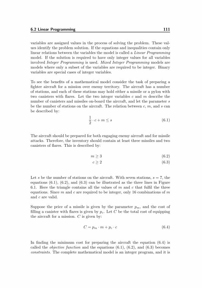
6.2 Linear Programming 111
variables are assigned values in the process of solving the problem. These val-ues identify the problem solution. If the equations and inequalities contain onlylinear relations between the variables the model is called a Linear Programmingmodel. If the solution is required to have only integer values for all variablesinvolved Integer Programming is used. Mixed Integer Programming models aremodels where only a subset of the variables are required to be integer. Binaryvariables are special cases of integer variables.
To see the benefits of a mathematical model consider the task of preparing afighter aircraft for a mission over enemy territory. The aircraft has a numberof stations, and each of these stations may hold either a missile or a pylon withtwo canisters with flares. Let the two integer variables c and m describe thenumber of canisters and missiles on-board the aircraft, and let the parameter sbe the number of stations on the aircraft. The relation between c, m, and s canbe described by:
1
2· c + m ≤ s (6.1)
The aircraft should be prepared for both engaging enemy aircraft and for missileattacks. Therefore, the inventory should contain at least three missiles and twocanisters of flares. This is described by:
m ≥ 3 (6.2)
c ≥ 2 (6.3)
Let s be the number of stations on the aircraft. With seven stations, s = 7, theequations (6.1), (6.2), and (6.3) can be illustrated as the three lines in Figure6.1. Here the triangle contains all the values of m and c that fulfil the threeequations. Since m and c are required to be integer, only 16 combinations of mand c are valid.
Suppose the price of a missile is given by the parameter pm, and the cost offilling a canister with flares is given by pc. Let C be the total cost of equippingthe aircraft for a mission. C is given by:
C = pm ·m + pc · c (6.4)
In finding the minimum cost for preparing the aircraft the equation (6.4) iscalled the objective function and the equations (6.1), (6.2), and (6.3) becomesconstraints. The complete mathematical model is an integer program, and it is
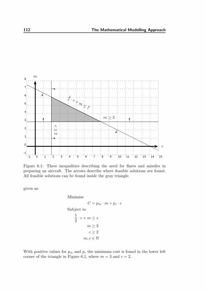
112 The Mathematical Modelling Approach
-1 0 1 2 3 4 5 6 7 8 9 10 11 12 13 14 15-1
0
1
2
3
4
5
6
7
8
c
m
m ≥ 3
c≥
2
12 · c + m
≤ 7
Figure 6.1: Three inequalities describing the need for flares and missiles inpreparing an aircraft. The arrows describe where feasible solutions are found.All feasible solutions can be found inside the gray triangle.
given as:
Minimise
C = pm ·m + pc · c
Subject to
1
2· c + m ≤ s
m ≥ 3
c ≥ 2
m, c ∈ N
With positive values for pm and pc the minimum cost is found in the lower leftcorner of the triangle in Figure 6.1, where m = 3 and c = 2.
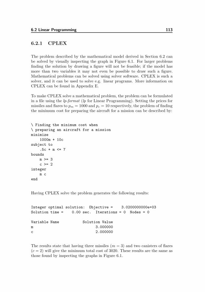
6.2 Linear Programming 113
6.2.1 CPLEX
The problem described by the mathematical model derived in Section 6.2 canbe solved by visually inspecting the graph in Figure 6.1. For larger problemsfinding the solution by drawing a figure will not be feasible; if the model hasmore than two variables it may not even be possible to draw such a figure.Mathematical problems can be solved using solver software. CPLEX is such asolver, and it can be used to solve e.g. linear programs. More information onCPLEX can be found in Appendix E.
To make CPLEX solve a mathematical problem, the problem can be formulatedin a file using the lp-format (lp for Linear Programming). Setting the prices formissiles and flares to pm = 1000 and pc = 10 respectively, the problem of findingthe minimum cost for preparing the aircraft for a mission can be described by:
\ Finding the minimum cost when
\ preparing an aircraft for a mission
minimize
1000m + 10c
subject to
.5c + m <= 7
bounds
m >= 3
c >= 2
integer
m c
end
Having CPLEX solve the problem generates the following results:
Integer optimal solution: Objective = 3.0200000000e+03
Solution time = 0.00 sec. Iterations = 0 Nodes = 0
Variable Name Solution Value
m 3.000000
c 2.000000
The results state that having three missiles (m = 3) and two canisters of flares(c = 2) will give the minimum total cost of 3020. These results are the same asthose found by inspecting the graphs in Figure 6.1.
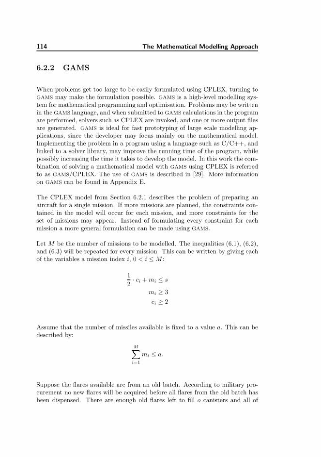
114 The Mathematical Modelling Approach
6.2.2 GAMS
When problems get too large to be easily formulated using CPLEX, turning toGAMS may make the formulation possible. GAMS is a high-level modelling sys-tem for mathematical programming and optimisation. Problems may be writtenin the GAMS language, and when submitted to GAMS calculations in the programare performed, solvers such as CPLEX are invoked, and one or more output filesare generated. GAMS is ideal for fast prototyping of large scale modelling ap-plications, since the developer may focus mainly on the mathematical model.Implementing the problem in a program using a language such as C/C++, andlinked to a solver library, may improve the running time of the program, whilepossibly increasing the time it takes to develop the model. In this work the com-bination of solving a mathematical model with GAMS using CPLEX is referredto as GAMS/CPLEX. The use of GAMS is described in [29]. More informationon GAMS can be found in Appendix E.
The CPLEX model from Section 6.2.1 describes the problem of preparing anaircraft for a single mission. If more missions are planned, the constraints con-tained in the model will occur for each mission, and more constraints for theset of missions may appear. Instead of formulating every constraint for eachmission a more general formulation can be made using GAMS.
Let M be the number of missions to be modelled. The inequalities (6.1), (6.2),and (6.3) will be repeated for every mission. This can be written by giving eachof the variables a mission index i, 0 < i ≤M :
1
2· ci + mi ≤ s
mi ≥ 3
ci ≥ 2
Assume that the number of missiles available is fixed to a value a. This can bedescribed by:
MXi=1
mi ≤ a.
Suppose the flares available are from an old batch. According to military pro-curement no new flares will be acquired before all flares from the old batch hasbeen dispensed. There are enough old flares left to fill o canisters and all of
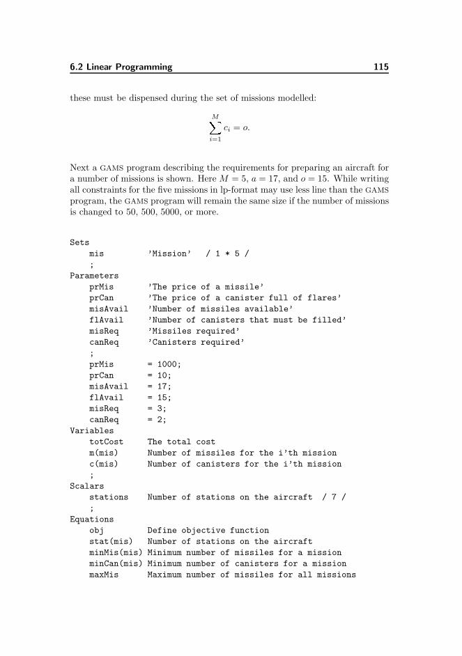
6.2 Linear Programming 115
these must be dispensed during the set of missions modelled:
MXi=1
ci = o.
Next a GAMS program describing the requirements for preparing an aircraft fora number of missions is shown. Here M = 5, a = 17, and o = 15. While writingall constraints for the five missions in lp-format may use less line than the GAMS
program, the GAMS program will remain the same size if the number of missionsis changed to 50, 500, 5000, or more.
Sets
mis ’Mission’ / 1 * 5 /
;
Parameters
prMis ’The price of a missile’
prCan ’The price of a canister full of flares’
misAvail ’Number of missiles available’
flAvail ’Number of canisters that must be filled’
misReq ’Missiles required’
canReq ’Canisters required’
;
prMis = 1000;
prCan = 10;
misAvail = 17;
flAvail = 15;
misReq = 3;
canReq = 2;
Variables
totCost The total cost
m(mis) Number of missiles for the i’th mission
c(mis) Number of canisters for the i’th mission
;
Scalars
stations Number of stations on the aircraft / 7 /
;
Equations
obj Define objective function
stat(mis) Number of stations on the aircraft
minMis(mis) Minimum number of missiles for a mission
minCan(mis) Minimum number of canisters for a mission
maxMis Maximum number of missiles for all missions
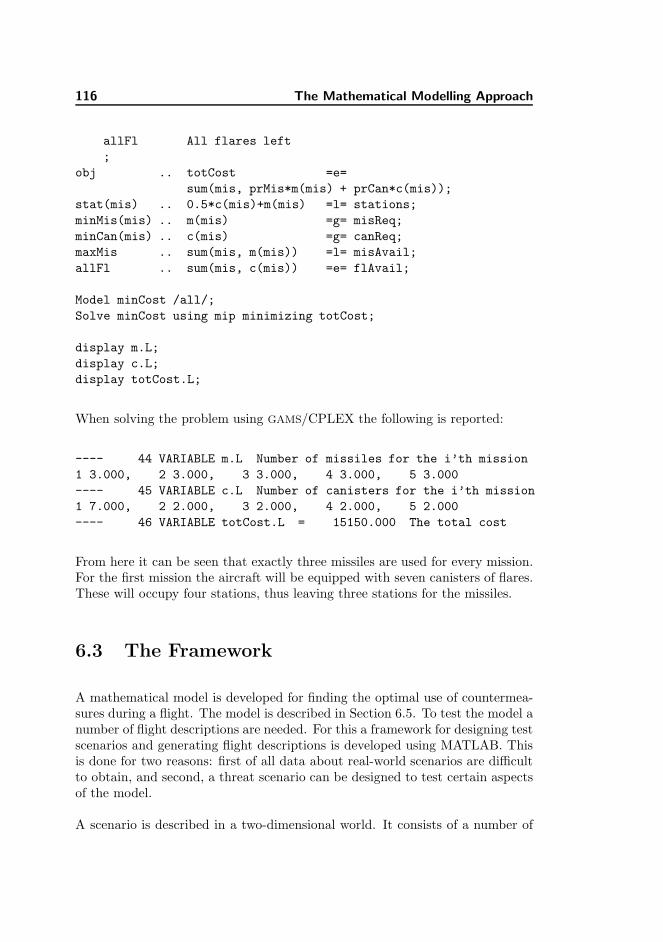
116 The Mathematical Modelling Approach
allFl All flares left
;
obj .. totCost =e=
sum(mis, prMis*m(mis) + prCan*c(mis));
stat(mis) .. 0.5*c(mis)+m(mis) =l= stations;
minMis(mis) .. m(mis) =g= misReq;
minCan(mis) .. c(mis) =g= canReq;
maxMis .. sum(mis, m(mis)) =l= misAvail;
allFl .. sum(mis, c(mis)) =e= flAvail;
Model minCost /all/;
Solve minCost using mip minimizing totCost;
display m.L;
display c.L;
display totCost.L;
When solving the problem using GAMS/CPLEX the following is reported:
---- 44 VARIABLE m.L Number of missiles for the i’th mission
1 3.000, 2 3.000, 3 3.000, 4 3.000, 5 3.000
---- 45 VARIABLE c.L Number of canisters for the i’th mission
1 7.000, 2 2.000, 3 2.000, 4 2.000, 5 2.000
---- 46 VARIABLE totCost.L = 15150.000 The total cost
From here it can be seen that exactly three missiles are used for every mission.For the first mission the aircraft will be equipped with seven canisters of flares.These will occupy four stations, thus leaving three stations for the missiles.
6.3 The Framework
A mathematical model is developed for finding the optimal use of countermea-sures during a flight. The model is described in Section 6.5. To test the model anumber of flight descriptions are needed. For this a framework for designing testscenarios and generating flight descriptions is developed using MATLAB. Thisis done for two reasons: first of all data about real-world scenarios are difficultto obtain, and second, a threat scenario can be designed to test certain aspectsof the model.
A scenario is described in a two-dimensional world. It consists of a number of
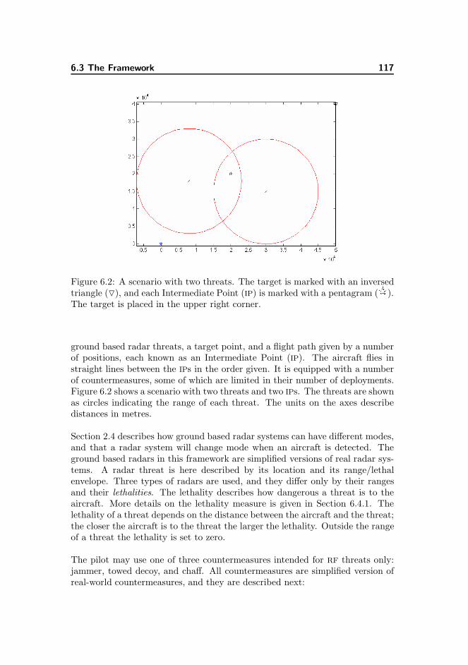
6.3 The Framework 117
Figure 6.2: A scenario with two threats. The target is marked with an inversedtriangle (O), and each Intermediate Point (IP) is marked with a pentagram (9).The target is placed in the upper right corner.
ground based radar threats, a target point, and a flight path given by a numberof positions, each known as an Intermediate Point (IP). The aircraft flies instraight lines between the IPs in the order given. It is equipped with a numberof countermeasures, some of which are limited in their number of deployments.Figure 6.2 shows a scenario with two threats and two IPs. The threats are shownas circles indicating the range of each threat. The units on the axes describedistances in metres.
Section 2.4 describes how ground based radar systems can have different modes,and that a radar system will change mode when an aircraft is detected. Theground based radars in this framework are simplified versions of real radar sys-tems. A radar threat is here described by its location and its range/lethalenvelope. Three types of radars are used, and they differ only by their rangesand their lethalities. The lethality describes how dangerous a threat is to theaircraft. More details on the lethality measure is given in Section 6.4.1. Thelethality of a threat depends on the distance between the aircraft and the threat;the closer the aircraft is to the threat the larger the lethality. Outside the rangeof a threat the lethality is set to zero.
The pilot may use one of three countermeasures intended for RF threats only:jammer, towed decoy, and chaff. All countermeasures are simplified version ofreal-world countermeasures, and they are described next:

118 The Mathematical Modelling Approach
The jammer works by obfuscating any nearby threats. It works on a threat if theaircraft is within the range of this threat. The jammer antenna is positioned soit offers the biggest reductions if the threat is placed either in front of or behindthe aircraft. When close to the threat the jammer offers no reduction in thethreat lethality. The reduction increases as the aircraft gets further away fromthe threat, and it reaches its peak when the aircraft is at the rim of the rangeof the threat.
At any time the jammer will be in one of four states: off; on but not yet active;on and active; and active while turning off. In the model the jammer has to bein one of these states for a given period of time, i.e. for a given number of timesteps, before its transition into the next state. No upper limits exist on the timethe jammer should be off before it is turned on, or for how long it must be activebefore being turned off. Turning the jammer on and off takes a preset period oftime, so a number of time steps is necessary on these transitional states. Thereis no limit to the number of times the jammer can be turned on. If it doesnot offer the best reductions it should not be turned on, since it may attractunnecessary attention from threats.
The towed decoy works basically as a ”jammer on a string”. One of the maindifferences between the on-board jammer and the towed decoy is the reductionsgiven by the use of the decoy. Since the decoy is towed behind the aircraft it hasthe highest effect when the aircraft is flying away from the threats. It will be inone of four states: off; on but not yet active; on and active; and severed whilethe system is settling. It takes time for the decoy to become active since thisrequires the unreeling of a wire connected to the decoy. The towed decoy willstop jamming as soon as it has been turned off. It is assumed that the jammermay continue to jam as long as it is not severed. While the jammer may beturned on and off as often as necessary the number of towed decoys on-boardthe aircraft is limited. When it is turned off the wire is cut and the decoy islost.
When chaff is dispensed it will form a cloud with a RCS comparable to that ofthe aircraft. Once formed, the cloud will maintain its RCS for a while. Chaff canbe dispensed even if a chaff cloud is already formed. The frequency of dispensingchaff is limited by a latency period between two contiguous dispensings and bythe amount of chaff available.
6.4 Optimise Survivability 119
6.4 Optimise Survivability
The aim of this work is to give the aircraft the highest probability of survivinga mission as possible. Determining the probability of surviving, PS , is not atrivial task, and a survivability measure, S, is introduced. No direct mappingbetween S and PS is given, but the one is given by a monotonous bijection fromthe other.
Determining a value of S over a time frame can be done by subdividing theframe into a number of time steps, calculating the value for each of these steps,and finally combining the values into a single value for that time frame. This isdescribed in the Sections 6.4.1 and 6.4.2. The optimal solution indicates wheneach of the available countermeasures must be activated. The usage is describedfor each of the time steps in the given time frame.
6.4.1 Lethality
The lethality experienced by the aircraft at any given time depends on thethreats given in the current scenario. Let T denote the number of time steps inthe time frame and let H be the number of threats in the current scenario. Atthe time t, 0 < t ≤ T , the lethality given by the threat h, 0 < h ≤ H is definedby three factors: the probability Pth of a ground based radar actually posing athreat to the aircraft, the threat lethality Lth, and finally the current lethalityreduction Rth for the threat which depends on e.g. the countermeasures in use.
Knowledge about the presence of a threat may be the result of intelligencereports or measurements done by on-board sensors. Both of these sources maybe more or less reliable, and the probability of a radar system posing a threatmay depend on the reliability of the source. A radar actually positioned in thescenario may also be out of function, thus not posing a threat.
The reduction of the lethality of threat h to the time t depends on two parame-ters: the angle towards the threat, αth and the distance between the threat andthe aircraft, ρth (see Figure 6.3). The distance between threat and aircraft ismeasured as a percentage of the threat range, and since a threat has no lethalityoutside its range the lethality is set to zero when ρth > 100%. In Figure 6.4 thereductions of lethality for the three countermeasures are shown as functions ofboth angle and distance.
The aircraft will always point in the direction of flight, i.e. towards the nextIP or the target. This is used when finding the angle between the aircraft
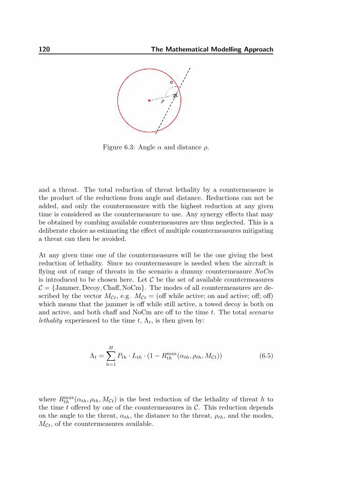
120 The Mathematical Modelling Approach
Figure 6.3: Angle α and distance ρ.
and a threat. The total reduction of threat lethality by a countermeasure isthe product of the reductions from angle and distance. Reductions can not beadded, and only the countermeasure with the highest reduction at any giventime is considered as the countermeasure to use. Any synergy effects that maybe obtained by combing available countermeasures are thus neglected. This is adeliberate choice as estimating the effect of multiple countermeasures mitigatinga threat can then be avoided.
At any given time one of the countermeasures will be the one giving the bestreduction of lethality. Since no countermeasure is needed when the aircraft isflying out of range of threats in the scenario a dummy countermeasure NoCmis introduced to be chosen here. Let C be the set of available countermeasuresC = {Jammer, Decoy, Chaff, NoCm}. The modes of all countermeasures are de-scribed by the vector MCt, e.g. MCt = (off while active; on and active; off; off)which means that the jammer is off while still active, a towed decoy is both onand active, and both chaff and NoCm are off to the time t. The total scenariolethality experienced to the time t, Λt, is then given by:
Λt =HX
h=1
Pth · Lth · (1 −Rmaxth (αth, ρth, MCt)) (6.5)
where Rmaxth (αth, ρth, MCt) is the best reduction of the lethality of threat h to
the time t offered by one of the countermeasures in C. This reduction dependson the angle to the threat, αth, the distance to the threat, ρth, and the modes,MCt, of the countermeasures available.
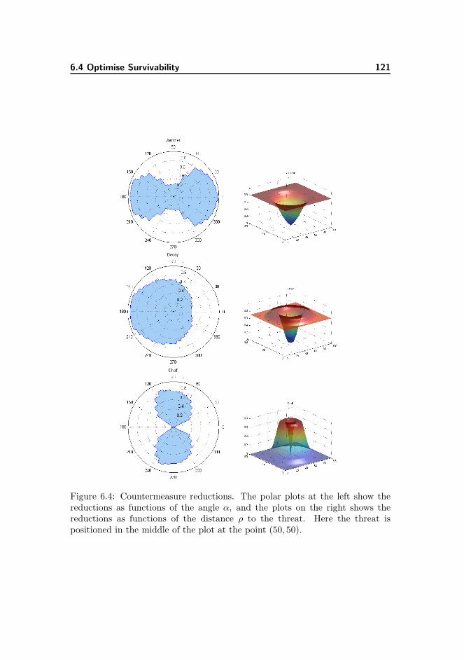
6.4 Optimise Survivability 121
Figure 6.4: Countermeasure reductions. The polar plots at the left show thereductions as functions of the angle α, and the plots on the right shows thereductions as functions of the distance ρ to the threat. Here the threat ispositioned in the middle of the plot at the point (50, 50).
122 The Mathematical Modelling Approach
6.4.2 Survivability
The relation between the lethality and the survivability at time t, St is heredefined as:
St = 1− Λt (6.6)
Since all factors in Λt have values between 0 and 1, both Λt and St will have val-ues between 0 and 1. As stated earlier the survivability should not be mistakenfor the probability of survival, as the scope of St suggests.
Finding an overall survivability measure by combining the survivabilities overtime can be done in numerous ways. One way is by integrating the survivabilityover time:
S =
ZT
Stdt (6.7)
Discretising the time frame into time steps, the combination of the survivabilitiesfrom each time step can be calculated as a sum:
Ssum =TX
t=1
St (6.8)
If the aircraft flies the entire time frame outside the range of any threat, thesurvivability in each time step is 1, and the sum of survivabilities then equalsthe number of time steps. Since this value will be more than one if more thanone time step is used, the analogy to the PS is lost. If Ssum is normalized bydividing it with the number of time steps in the time frame, it will have a valuebetween 0 and 1, and the analogy to the probability of survival is regained:
Ssum,norm =1
T
TXt=1
St (6.9)
Optimising Ssum may not ensure the aircraft the highest probability of surviv-ing. In Figure 6.5 two courses with different development in scenario lethalityare compared. The graph in Figure 6.5(a) shows varying scenario lethality asa function of time. This scenario lethality may be the result of the aircraftapproaching a threat without any active countermeasures, which gives the risein lethality. At some point in time the jammer may be turned on, which resultsin a decline in scenario lethality. In Figure 6.5(b) the scenario lethality is keptroughly constant, e.g. due to an active jammer. If the time steps are keptsufficiently small Ssum is comparable to the area under the graphs. The area in
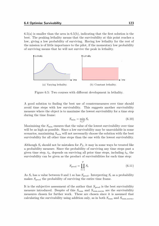
6.4 Optimise Survivability 123
6.5(a) is smaller than the area in 6.5(b), indicating that the first solution is thebest. The peaking lethality means that the survivability at this point reaches alow, giving a low probability of surviving. Having low lethality for the rest ofthe mission is of little importance to the pilot, if the momentary low probabilityof surviving means that he will not survive the peak in lethality.
(a) Varying lethality. (b) Constant lethality.
Figure 6.5: Two courses with different development in lethality.
A good solution to finding the best use of countermeasures over time shouldavoid time steps with low survivability. This suggests another survivabilitymeasure where the object is to maximise the lowest survivability for a time stepduring the time frame:
Smin = mint≤T
St (6.10)
Maximising the Smin ensures that the value of the lowest survivability over timewill be as high as possible. Since a low survivability may be unavoidable in somescenarios, maximising Smin will not necessarily choose the solution with the bestsurvivability for all other time steps than the one with the lowest survivability.
Although St should not be mistaken for PS , it may in some ways be treated likea probability measure. Since the probability of surviving any time steps past agiven time step, t0, depends on surviving all prior time steps, including t0, thesurvivability can be given as the product of survivabilities for each time step:
Sprod =TY
t=1
St (6.11)
As St has a value between 0 and 1 so has Sprod. Interpreting St as a probabilitymakes Sprod the probability of surviving the entire time frame.
It is the subjective assessment of the author that Sprod is the best survivabilitymeasure introduced. Despite of this Ssum and Ssum,norm are the survivabilitymeasures chosen for further work. These are chosen since it is assumed thatcalculating the survivability using addition only, as in both Ssum and Ssum,norm,
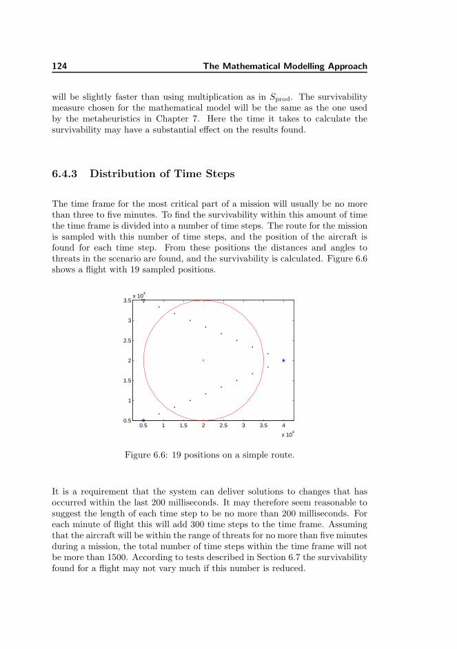
124 The Mathematical Modelling Approach
will be slightly faster than using multiplication as in Sprod. The survivabilitymeasure chosen for the mathematical model will be the same as the one usedby the metaheuristics in Chapter 7. Here the time it takes to calculate thesurvivability may have a substantial effect on the results found.
6.4.3 Distribution of Time Steps
The time frame for the most critical part of a mission will usually be no morethan three to five minutes. To find the survivability within this amount of timethe time frame is divided into a number of time steps. The route for the missionis sampled with this number of time steps, and the position of the aircraft isfound for each time step. From these positions the distances and angles tothreats in the scenario are found, and the survivability is calculated. Figure 6.6shows a flight with 19 sampled positions.
0.5 1 1.5 2 2.5 3 3.5 4
x 104
0.5
1
1.5
2
2.5
3
3.5x 10
4
Figure 6.6: 19 positions on a simple route.
It is a requirement that the system can deliver solutions to changes that hasoccurred within the last 200 milliseconds. It may therefore seem reasonable tosuggest the length of each time step to be no more than 200 milliseconds. Foreach minute of flight this will add 300 time steps to the time frame. Assumingthat the aircraft will be within the range of threats for no more than five minutesduring a mission, the total number of time steps within the time frame will notbe more than 1500. According to tests described in Section 6.7 the survivabilityfound for a flight may not vary much if this number is reduced.
6.4 Optimise Survivability 125
The time steps in this work are distributed evenly over the time frame. Whilethis makes the sampling of location points easy it may not be the best way todistribute the time steps. If the aircraft is within the lethal range of a threatthe pilot must focus on this threat for more reasons: if he does not survive theencounter with this threat he will not survive encounters with future threatseither, and the probability of this threat actually posing a threat is likely tobe higher than for any threats that may or may not be encountered later on.Focussing on threats in the near future may be reflected in the distribution oftime steps. This can be done by sampling the first period of time, e.g. the next30 seconds, with a higher frequency, the next couple of minutes with a lowerfrequency, and finally having only a few samples in the last part of the timeframe.
Keeping the focus on the actions in the near future can also be done by weight-ing contributions from early time steps higher in the survivability measure. Thiscan e.g. be done in the estimation of the probability for each threat. Like withthe unevenly distribution mentioned before meeting threats in the far futurewill have only minor influence on the survivability found. The down side tothis approach is that the benefit from optimising the use of expendable counter-measures may be reduced. This has to be considered when introducing eitheruneven distribution or weighing of time steps.
6.4.4 Deployment Scheme
A solution to the problem of finding the best use of countermeasures takes theform of a deployment scheme. In a deployment scheme two columns describeeach of the countermeasures. The one column indicates the time steps in wherethe countermeasure is active and the other column describes when the counter-measure is turned on/dispensed. Figure 6.7 shows such a deployment scheme.
When a countermeasure is active it will remain so for a number of time steps.Each of these collections of time steps is called a deployment interval. For thetowed decoy the maximum number of deployment intervals equals the numberof decoys on-board the aircraft. If the towed decoy is not needed for a shortperiod of time during flight, it may be necessary to keep it active to avoid usingmore decoys than are available. For chaff a deployment interval can consist ofmore chaff dispensings.
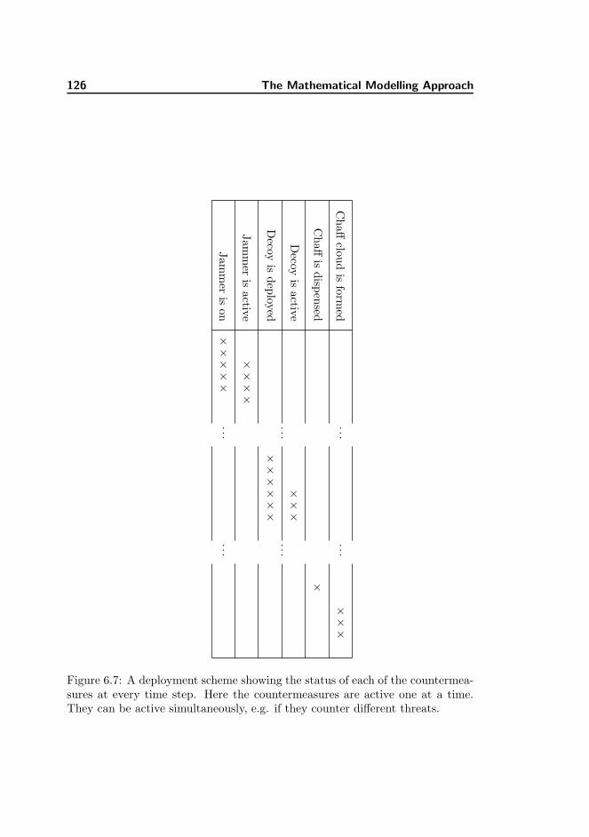
126 The Mathematical Modelling Approach
Jam
mer
ison
Jam
mer
isactiv
e
Decoy
isdep
loyed
Decoy
isactiv
e
Chaff
isdisp
ensed
Chaff
cloud
isfo
rmed
×××××
××××
......
...
××××××
×××
......
...
×
×××
Figure 6.7: A deployment scheme showing the status of each of the countermea-sures at every time step. Here the countermeasures are active one at a time.They can be active simultaneously, e.g. if they counter different threats.
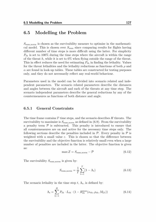
6.5 Modelling the Problem 127
6.5 Modelling the Problem
Ssum,norm is chosen as the survivability measure to optimise in the mathemati-cal model. This is chosen over Ssum since comparing results for flights havingdifferent number of time steps is more difficult using the latter. For simplicityPth is set to 100% during the time steps where the aircraft is within the rangeof the threat h, while it is set to 0% when flying outside the range of the threat.This in effect reduces the need for estimating Pth in finding the lethality. Valuesfor the threat lethalities and the lethality reductions as functions of both ρ andα are found in look-up tables. These tables are constructed for testing purposesonly, and they do not necessarily reflect any real-world behaviour.
Parameters used in the model can be divided into scenario related and inde-pendent parameters. The scenario related parameters describe the distancesand angles between the aircraft and each of the threats at any time step. Thescenario independent parameters describe the general reductions by any of thecountermeasures as functions of both distance and angle.
6.5.1 General Constraints
The time frame contains T time steps, and the scenario describes H threats. Thesurvivability to maximize is Ssum,norm as defined in (6.9). From the survivabilitya penalty term P is subtracted. This penalty is introduced to ensure thatall countermeasures are on and active for the necessary time steps only. Thefollowing sections describe the penalties included in P . Every penalty in P isweighted with a small value ε. This is chosen so that the difference betweenthe survivability and the objective function is relatively small even when a largenumber of penalties are included in the latter. The objective function is givenas:
max Z = Ssum,norm − P (6.12)
The survivability Ssum,norm is given by:
Ssum,norm =1
T
TXt=1
(1 − Λt) (6.13)
The scenario lethality in the time step t, Λt, is defined by:
Λt =HX
h=1
Pth · Lth · (1−Rmaxth (αth, ρth, MCt)) (6.14)
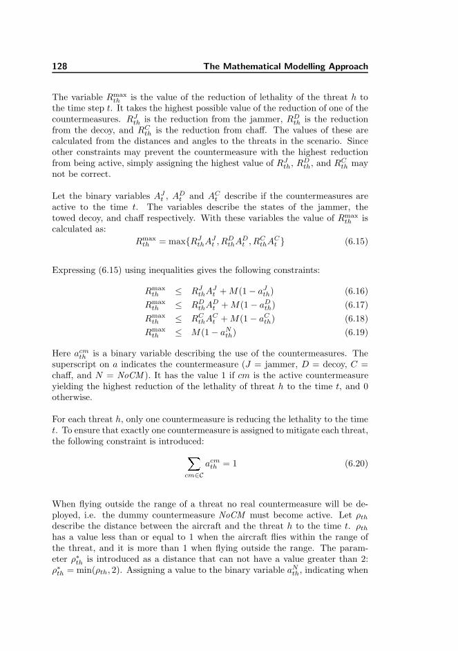
128 The Mathematical Modelling Approach
The variable Rmaxth is the value of the reduction of lethality of the threat h to
the time step t. It takes the highest possible value of the reduction of one of thecountermeasures. RJ
th is the reduction from the jammer, RDth is the reduction
from the decoy, and RCth is the reduction from chaff. The values of these are
calculated from the distances and angles to the threats in the scenario. Sinceother constraints may prevent the countermeasure with the highest reductionfrom being active, simply assigning the highest value of RJ
th, RDth, and RC
th maynot be correct.
Let the binary variables AJt , AD
t and ACt describe if the countermeasures are
active to the time t. The variables describe the states of the jammer, thetowed decoy, and chaff respectively. With these variables the value of Rmax
th iscalculated as:
Rmaxth = max{RJ
thAJt , RD
thADt , RC
thACt } (6.15)
Expressing (6.15) using inequalities gives the following constraints:
Rmaxth ≤ RJ
thAJt + M(1− aJ
th) (6.16)
Rmaxth ≤ RD
thADt + M(1− aD
th) (6.17)
Rmaxth ≤ RC
thACt + M(1− aC
th) (6.18)
Rmaxth ≤ M(1− aN
th) (6.19)
Here acmth is a binary variable describing the use of the countermeasures. The
superscript on a indicates the countermeasure (J = jammer, D = decoy, C =chaff, and N = NoCM ). It has the value 1 if cm is the active countermeasureyielding the highest reduction of the lethality of threat h to the time t, and 0otherwise.
For each threat h, only one countermeasure is reducing the lethality to the timet. To ensure that exactly one countermeasure is assigned to mitigate each threat,the following constraint is introduced:X
cm∈C
acmth = 1 (6.20)
When flying outside the range of a threat no real countermeasure will be de-ployed, i.e. the dummy countermeasure NoCM must become active. Let ρth
describe the distance between the aircraft and the threat h to the time t. ρth
has a value less than or equal to 1 when the aircraft flies within the range ofthe threat, and it is more than 1 when flying outside the range. The param-eter ρ∗th is introduced as a distance that can not have a value greater than 2:ρ∗th = min(ρth, 2). Assigning a value to the binary variable aN
th, indicating when
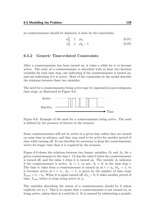
6.5 Modelling the Problem 129
no countermeasure should be deployed, is done by the constraints:
aNth ≤ ρth (6.21)
aNth ≥ ρ∗th − 1 (6.22)
6.5.2 Generic Time-related Constraints
After a countermeasure has been turned on, it takes a while for it to becomeactive. The state of a countermeasure is described with at least two decisionvariables for each time step, one indicating if the countermeasure is turned on,and one indicating if it is active. Most of the constraints in the model describethe relations between these two variables.
The need for a countermeasure being active may be expressed in non-contiguoustime steps, as illustrated in Figure 6.8.
Time
Active
Inactive
Figure 6.8: Example of the need for a countermeasure being active. The needis defined by the presence of threats in the scenario.
Some countermeasures will not be active to a given time unless they are turnedon some time in advance, and they may need to be active for another period oftime while turning off. It can therefore be necessary to keep the countermeasureactive for longer time than it is required by the scenario.
Figure 6.9 shows the relations between two binary variables, Ot and At, for agiven countermeasure to the time t. Ot has the value 0 when the countermeasureis turned off, and the value 1 when it is turned on. The variable At indicatesif the countermeasure is active, At = 1, or not, At = 0, in the time step t.The time it takes from a countermeasure is turned on at t = t0, Ot0 = 1, toit becomes active at t = t1, At1 = 1, is given by the number of time stepsTstart = t1 − t0. When it is again turned off, Ot2 = 0, it takes another period oftime, Tend, before it stops being active at t3.
The variables describing the status of a countermeasure should be 0 unlessexplicitly set to 1. This is to ensure that a countermeasure is not turned on, orbeing active, unless there is a need for it. It is ensured by subtracting a penalty
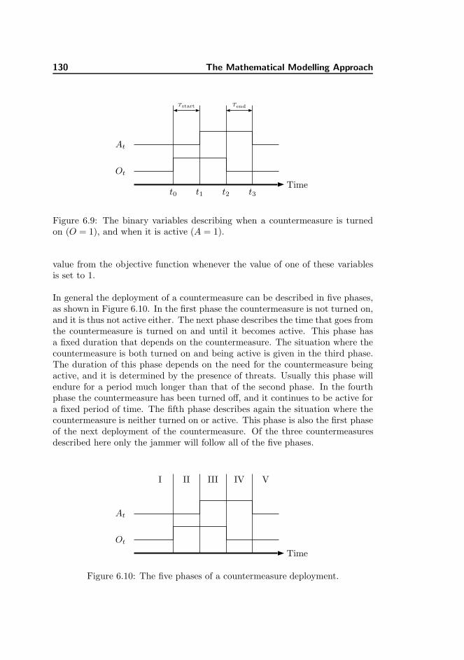
130 The Mathematical Modelling Approach
Time
At
Ot
t0 t1 t2 t3
Tstart Tend
Figure 6.9: The binary variables describing when a countermeasure is turnedon (O = 1), and when it is active (A = 1).
value from the objective function whenever the value of one of these variablesis set to 1.
In general the deployment of a countermeasure can be described in five phases,as shown in Figure 6.10. In the first phase the countermeasure is not turned on,and it is thus not active either. The next phase describes the time that goes fromthe countermeasure is turned on and until it becomes active. This phase hasa fixed duration that depends on the countermeasure. The situation where thecountermeasure is both turned on and being active is given in the third phase.The duration of this phase depends on the need for the countermeasure beingactive, and it is determined by the presence of threats. Usually this phase willendure for a period much longer than that of the second phase. In the fourthphase the countermeasure has been turned off, and it continues to be active fora fixed period of time. The fifth phase describes again the situation where thecountermeasure is neither turned on or active. This phase is also the first phaseof the next deployment of the countermeasure. Of the three countermeasuresdescribed here only the jammer will follow all of the five phases.
Time
At
Ot
I II III IV V
Figure 6.10: The five phases of a countermeasure deployment.
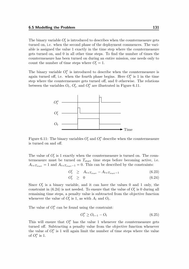
6.5 Modelling the Problem 131
The binary variable O′t is introduced to describes when the countermeasure gets
turned on, i.e. when the second phase of the deployment commences. The vari-able is assigned the value 1 exactly in the time step where the countermeasuregets turned on, and 0 in all other time steps. To find the number of times thecountermeasure has been turned on during an entire mission, one needs only tocount the number of time steps where O′
t = 1.
The binary variable O′′t is introduced to describe when the countermeasure is
again turned off, i.e. when the fourth phase begins. Here O′′t is 1 in the time
step where the countermeasure gets turned off, and 0 otherwise. The relationsbetween the variables Ot, O′
t, and O′′t are illustrated in Figure 6.11.
Time
O′′t
O′t
Ot
Figure 6.11: The binary variables O′t and O′′
t describe when the countermeasureis turned on and off.
The value of O′t is 1 exactly when the countermeasure is turned on. The coun-
termeasure must be turned on Tstart time steps before becoming active, i.e.At+Tstart = 1 and At+Tstart−1 = 0. This can be described by the constraints:
O′t ≥ At+Tstart − At+Tstart−1 (6.23)
O′t ≥ 0 (6.24)
Since O′t is a binary variable, and it can have the values 0 and 1 only, the
constraint in (6.24) is not needed. To ensure that the value of O′t is 0 during all
remaining time steps, a penalty value is subtracted from the objective functionwhenever the value of O′
t is 1, as with At and Ot.
The value of O′′t can be found using the constraint:
O′′t ≥ Ot−1 −Ot (6.25)
This will ensure that O′′t has the value 1 whenever the countermeasure gets
turned off. Subtracting a penalty value from the objective function wheneverthe value of O′′
t is 1 will again limit the number of time steps where the valueof O′′
t is 1.
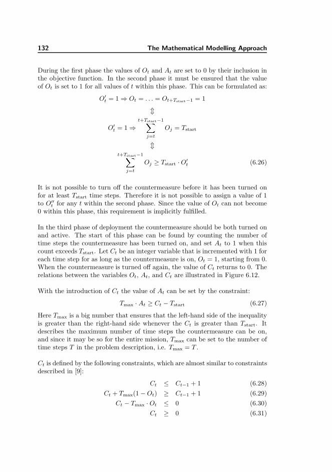
132 The Mathematical Modelling Approach
During the first phase the values of Ot and At are set to 0 by their inclusion inthe objective function. In the second phase it must be ensured that the valueof Ot is set to 1 for all values of t within this phase. This can be formulated as:
O′t = 1⇒ Ot = . . . = Ot+Tstart−1 = 1
m
O′t = 1⇒
t+Tstart−1Xj=t
Oj = Tstart
m
t+Tstart−1Xj=t
Oj ≥ Tstart ·O′t (6.26)
It is not possible to turn off the countermeasure before it has been turned onfor at least Tstart time steps. Therefore it is not possible to assign a value of 1to O′′
t for any t within the second phase. Since the value of Ot can not become0 within this phase, this requirement is implicitly fulfilled.
In the third phase of deployment the countermeasure should be both turned onand active. The start of this phase can be found by counting the number oftime steps the countermeasure has been turned on, and set At to 1 when thiscount exceeds Tstart. Let Ct be an integer variable that is incremented with 1 foreach time step for as long as the countermeasure is on, Ot = 1, starting from 0.When the countermeasure is turned off again, the value of Ct returns to 0. Therelations between the variables Ot, At, and Ct are illustrated in Figure 6.12.
With the introduction of Ct the value of At can be set by the constraint:
Tmax ·At ≥ Ct − Tstart (6.27)
Here Tmax is a big number that ensures that the left-hand side of the inequalityis greater than the right-hand side whenever the Ct is greater than Tstart. Itdescribes the maximum number of time steps the countermeasure can be on,and since it may be so for the entire mission, Tmax can be set to the number oftime steps T in the problem description, i.e. Tmax = T .
Ct is defined by the following constraints, which are almost similar to constraintsdescribed in [9]:
Ct ≤ Ct−1 + 1 (6.28)
Ct + Tmax(1−Ot) ≥ Ct−1 + 1 (6.29)
Ct − Tmax ·Ot ≤ 0 (6.30)
Ct ≥ 0 (6.31)
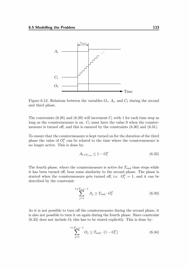
6.5 Modelling the Problem 133
Time
At
Ct
. ..
Ot
Tstart
Figure 6.12: Relations between the variables Ot, At, and Ct during the secondand third phase.
The constraints (6.28) and (6.29) will increment Ct with 1 for each time step aslong as the countermeasure is on. Ct must have the value 0 when the counter-measure is turned off, and this is ensured by the constraints (6.30) and (6.31).
To ensure that the countermeasure is kept turned on for the duration of the thirdphase the value of O′′
t can be related to the time where the countermeasure isno longer active. This is done by:
At+Tend≤ 1−O′′
t (6.32)
The fourth phase, where the countermeasure is active for Tend time steps whileit has been turned off, bear some similarity to the second phase. The phase isstarted when the countermeasure gets turned off, i.e. O′′
t = 1, and it can bedescribed by the constraint:
t+Tend−1Xj=t
Aj ≥ Tend ·O′′t (6.33)
As it is not possible to turn off the countermeasure during the second phase, itis also not possible to turn it on again during the fourth phase. Since constraint(6.33) does not include Ot this has to be stated explicitly. This is done by:
t+Tend−1Xj=t
Oj ≤ Tend · (1−O′′t ) (6.34)
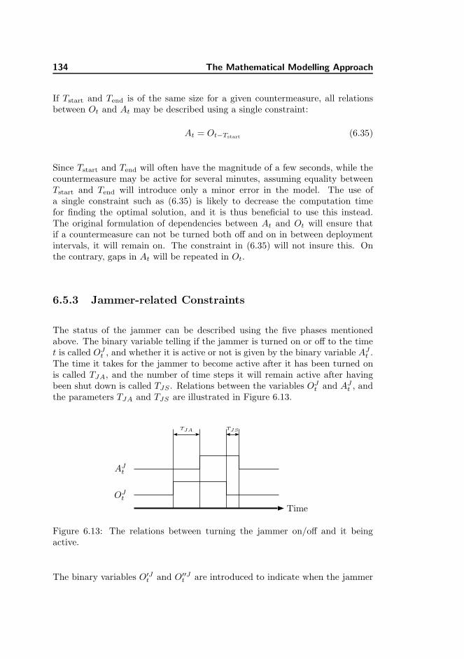
134 The Mathematical Modelling Approach
If Tstart and Tend is of the same size for a given countermeasure, all relationsbetween Ot and At may be described using a single constraint:
At = Ot−Tstart (6.35)
Since Tstart and Tend will often have the magnitude of a few seconds, while thecountermeasure may be active for several minutes, assuming equality betweenTstart and Tend will introduce only a minor error in the model. The use ofa single constraint such as (6.35) is likely to decrease the computation timefor finding the optimal solution, and it is thus beneficial to use this instead.The original formulation of dependencies between At and Ot will ensure thatif a countermeasure can not be turned both off and on in between deploymentintervals, it will remain on. The constraint in (6.35) will not insure this. Onthe contrary, gaps in At will be repeated in Ot.
6.5.3 Jammer-related Constraints
The status of the jammer can be described using the five phases mentionedabove. The binary variable telling if the jammer is turned on or off to the timet is called OJ
t , and whether it is active or not is given by the binary variable AJt .
The time it takes for the jammer to become active after it has been turned onis called TJA, and the number of time steps it will remain active after havingbeen shut down is called TJS . Relations between the variables OJ
t and AJt , and
the parameters TJA and TJS are illustrated in Figure 6.13.
Time
AJt
OJt
TJA TJS
Figure 6.13: The relations between turning the jammer on/off and it beingactive.
The binary variables O′Jt and O′′J
t are introduced to indicate when the jammer
6.5 Modelling the Problem 135
is turned on and off, respectively. They are defined by the constraints:
O′Jt ≥ AJ
t+TJA−AJ
t+TJA−1 (6.36)
O′′Jt ≥ OJ
t−1 −OJt (6.37)
Both OJt and AJ
t are included in the objective function, and their values duringthe first phase are thus set to 0. In the second phase the jammer has beenturned on and it can not be turned off for TJA time steps. This is controlled bythe constraint:
t+TJA−1Xj=t
OJj ≥ TJA ·O
′Jt (6.38)
In the third phase the value of AJt is controlled by the integer variable CJ
t whichcounts the number of time steps since the jammer was turned on. Keeping thecountermeasure turned on, the definition of CJ
t , and the relation between CJt
and AJt are given by the constraints:
CJt ≤ CJ
t−1 + 1 (6.39)
CJt + T (1−OJ
t ) ≥ CJt−1 + 1 (6.40)
CJt − T ·OJ
t ≤ 0 (6.41)
CJt ≥ 0 (6.42)
T ·AJt ≥ CJ
t − TJA (6.43)
AJt+TJS
≤ 1−O′′Jt (6.44)
(6.45)
The fourth phase begins when the jammer is shut down. This phase enduresfor TJS time steps during which the jammer will remain active, AJ
t = 1, whileit can not be turned on again, OJ
t = 0. This is described by the constraints:
t+TJS−1Xj=t
AJj ≥ TJS ·O
′′Jt (6.46)
t+TJS−1Xj=t
OJj ≤ TJS · (1−O′′J
t ) (6.47)
6.5.4 Decoy-related Constraints
As with the jammer the towed decoy will become active some time after it hasbeen deployed. A difference between the jammer and the decoy is, that the
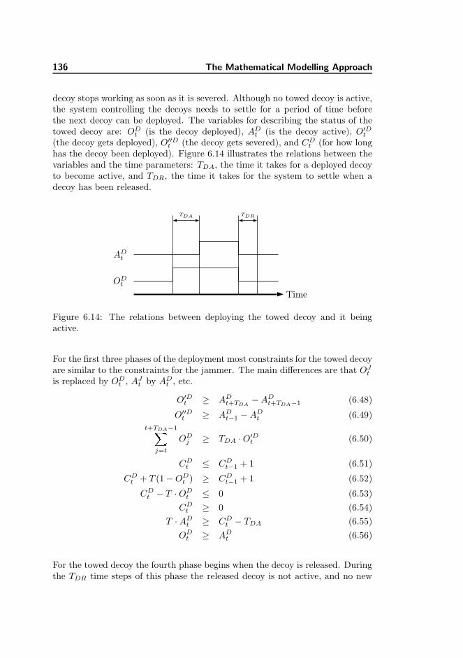
136 The Mathematical Modelling Approach
decoy stops working as soon as it is severed. Although no towed decoy is active,the system controlling the decoys needs to settle for a period of time beforethe next decoy can be deployed. The variables for describing the status of thetowed decoy are: OD
t (is the decoy deployed), ADt (is the decoy active), O′D
t
(the decoy gets deployed), O′′Dt (the decoy gets severed), and CD
t (for how longhas the decoy been deployed). Figure 6.14 illustrates the relations between thevariables and the time parameters: TDA, the time it takes for a deployed decoyto become active, and TDR, the time it takes for the system to settle when adecoy has been released.
Time
ADt
ODt
TDA TDR
Figure 6.14: The relations between deploying the towed decoy and it beingactive.
For the first three phases of the deployment most constraints for the towed decoyare similar to the constraints for the jammer. The main differences are that OJ
t
is replaced by ODt , AJ
t by ADt , etc.
O′Dt ≥ AD
t+TDA−AD
t+TDA−1 (6.48)
O′′Dt ≥ AD
t−1 −ADt (6.49)
t+TDA−1Xj=t
ODj ≥ TDA ·O
′Dt (6.50)
CDt ≤ CD
t−1 + 1 (6.51)
CDt + T (1−OD
t ) ≥ CDt−1 + 1 (6.52)
CDt − T ·OD
t ≤ 0 (6.53)
CDt ≥ 0 (6.54)
T · ADt ≥ CD
t − TDA (6.55)
ODt ≥ AD
t (6.56)
For the towed decoy the fourth phase begins when the decoy is released. Duringthe TDR time steps of this phase the released decoy is not active, and no new
6.5 Modelling the Problem 137
decoy can be deployed. Having a penalty value subtracted from the objectivefunction for each time step t in which AD
t = 1 will ensure that the decoy is notset as active during this phase. That no new decoy gets deployed is ensured by:
t+TDR−1Xj=t
ODj ≤ TDR · (1−O′′D
t ) (6.57)
A maximum of KD towed decoys can be deployed during the mission. SinceO′D
t has the value 1 each time a decoy gets deployed, this is given by:
TXt=1
O′Dt ≤ KD (6.58)
6.5.5 Chaff-related Constraints
The dispensing of chaff will not follow the five phases of countermeasure deploy-ment previously presented. Dispensing of chaff is initiated during a single timestep, and after a short period of time a chaff cloud is formed behind the aircraft.This cloud will last for another period of time before being dissipated. Afterdispensing chaff the next dispense may take place after a short latency period,regardless of whether the first cloud is yet formed, or if the effect of it has gone.The binary variables OC
t and ACt describes the use of chaff to the time t. OC
t
is 1 only during the time steps where chaff dispensing is initiated, and ACt is 1
when a chaff cloud is formed and potentially having an effect.
Three parameters describe the periods of time involved in chaff dispensing.TCF is the time it takes for a chaff cloud to be formed after chaff dispensing isinitiated, TCD denotes the duration of a chaff cloud, before it is dissipated, andTCL is the latency between contiguous chaff dispensings. The relations betweenthese parameters and the variables OC
t and ACt are illustrated in Figure 6.15
When chaff is dispensed, the chaff cloud will be formed after TCA time steps,and it will dissipate after another TCD time steps. This can be expressed as:
OCt = 1⇒ AC
t+TCF= . . . = AC
t+TCF +TCD−1 = 1
m
OCt = 1⇒
t+TCF +TCD−1Xj=t+TCF
ACj = TCD
m
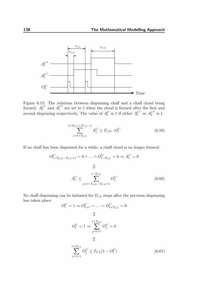
138 The Mathematical Modelling Approach
Time
AC2
t
AC1
t
OCt
TCF
TCL TCD
Figure 6.15: The relations between dispensing chaff and a chaff cloud beingformed. AC1
t and AC3
t are set to 1 when the cloud is formed after the first and
second dispensing respectively. The value of ACt is 1 if either AC1
t or AC2
t is 1.
t+TCF +TCD−1Xj=t+TCF
ACj ≥ TCD ·O
Ct (6.59)
If no chaff has been dispensed for a while, a chaff cloud is no longer formed:
OCt−TCD−TCF +1 = 0 ∧ . . . ∧OC
t−TCF= 0⇒ AC
t = 0
m
ACt ≤
t−TCFXj=t−TCD−TCF +1
OCj (6.60)
No chaff dispensing can be initiated for TCL steps after the previous dispensinghas taken place:
OCt = 1⇒ OC
t+1 = . . . = OCt+TCL
= 0
m
OCt = 1⇒
t+TCLXj=t+1
OCj = 0
m
t+TCLXj=t+1
OCj ≤ TCL(1−OC
t ) (6.61)
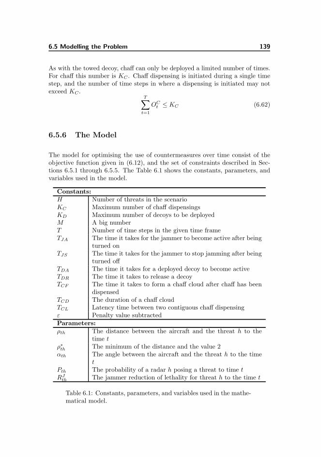
6.5 Modelling the Problem 139
As with the towed decoy, chaff can only be deployed a limited number of times.For chaff this number is KC . Chaff dispensing is initiated during a single timestep, and the number of time steps in where a dispensing is initiated may notexceed KC .
TXt=1
OCt ≤ KC (6.62)
6.5.6 The Model
The model for optimising the use of countermeasures over time consist of theobjective function given in (6.12), and the set of constraints described in Sec-tions 6.5.1 through 6.5.5. The Table 6.1 shows the constants, parameters, andvariables used in the model.
Constants:H Number of threats in the scenarioKC Maximum number of chaff dispensingsKD Maximum number of decoys to be deployedM A big numberT Number of time steps in the given time frameTJA The time it takes for the jammer to become active after being
turned onTJS The time it takes for the jammer to stop jamming after being
turned offTDA The time it takes for a deployed decoy to become activeTDR The time it takes to release a decoyTCF The time it takes to form a chaff cloud after chaff has been
dispensedTCD The duration of a chaff cloudTCL Latency time between two contiguous chaff dispensingε Penalty value subtractedParameters:ρth The distance between the aircraft and the threat h to the
time tρ∗th The minimum of the distance and the value 2αth The angle between the aircraft and the threat h to the time
tPth The probability of a radar h posing a threat to time tRJ
th The jammer reduction of lethality for threat h to the time t
Table 6.1: Constants, parameters, and variables used in the mathe-matical model.
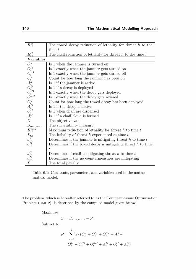
140 The Mathematical Modelling Approach
RDth The towed decoy reduction of lethality for threat h to the
time tRC
th The chaff reduction of lethality for threat h to the time tVariables:OJ
t Is 1 when the jammer is turned onO′J
t Is 1 exactly when the jammer gets turned onO′′J
t Is 1 exactly when the jammer gets turned offCJ
t Count for how long the jammer has been onAJ
t Is 1 if the jammer is activeOD
t Is 1 if a decoy is deployedO′D
t Is 1 exactly when the decoy gets deployedO′′D
t Is 1 exactly when the decoy gets severedCJ
t Count for how long the towed decoy has been deployedAD
t Is 1 if the decoy is activeOC
t Is 1 when chaff are dispensedAC
t Is 1 if a chaff cloud is formedZ The objective valueSsum,norm The survivability measureRmax
th Maximum reduction of lethality for threat h to time tLth The lethality of threat h experienced at time taJ
th Determines if the jammer is mitigating threat h to time taD
th Determines if the towed decoy is mitigating threat h to timet
aCth Determines if chaff is mitigating threat h to time t
aNth Determines if the no countermeasures are mitigatingP The total penalty
Table 6.1: Constants, parameters, and variables used in the mathe-matical model.
The problem, which is hereafter referred to as the Countermeasure OptimisationProblem (CMOP), is described by the compiled model given below.
Maximize
Z = Ssum,norm − P
Subject to
P =TX
t=1
ε · (OJt + O′J
t + O′′Jt + AJ
t +
ODt + O′D
t + O′′Dt + AD
t + OCt + AC
t )
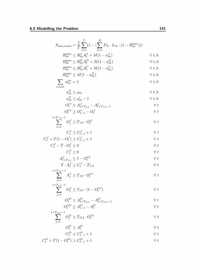
6.5 Modelling the Problem 141
Ssum,norm =1
T
TXt=1
(1 − (HX
h=1
Pth · Lth · (1−Rmaxth )))
Rmaxth ≤ RJ
thAJt + M(1− aJ
th) ∀ t, h
Rmaxth ≤ RD
thADt + M(1− aD
th) ∀ t, h
Rmaxth ≤ RC
thACt + M(1− aC
th) ∀ t, h
Rmaxth ≤M(1− aN
th) ∀ t, hXcm∈C
acmth = 1 ∀ t, h
aNth ≤ ρth ∀ t, h
aNth ≥ ρ∗th − 1 ∀ t, h
O′Jt ≥ AJ
t+TJA−AJ
t+TJA−1 ∀ t
O′′Jt ≥ OJ
t−1 −OJt ∀ t
t+TJA−1Xj=t
OJj ≥ TJA ·O
′Jt ∀ t
CJt ≤ CJ
t−1 + 1 ∀ t
CJt + T (1−OJ
t ) ≥ CJt−1 + 1 ∀ t
CJt − T ·OJ
t ≤ 0 ∀ t
CJt ≥ 0 ∀ t
AJt+TJS
≤ 1−O′′Jt ∀ t
T ·AJt ≥ CJ
t − TJA ∀ t
t+TJS−1Xj=t
AJj ≥ TJS ·O
′′Jt ∀ t
t+TJS−1Xj=t
OJj ≤ TJS · (1 −O′′J
t ) ∀ t
O′Dt ≥ AD
t+TDA−AD
t+TDA−1 ∀ t
O′′Dt ≥ AD
t−1 −ADt ∀ t
t+TDA−1Xj=t
ODj ≥ TDA ·O
′Dt ∀ t
ODt ≥ AD
t ∀ t
CDt ≤ CD
t−1 + 1 ∀ t
CDt + T (1−OD
t ) ≥ CDt−1 + 1 ∀ t
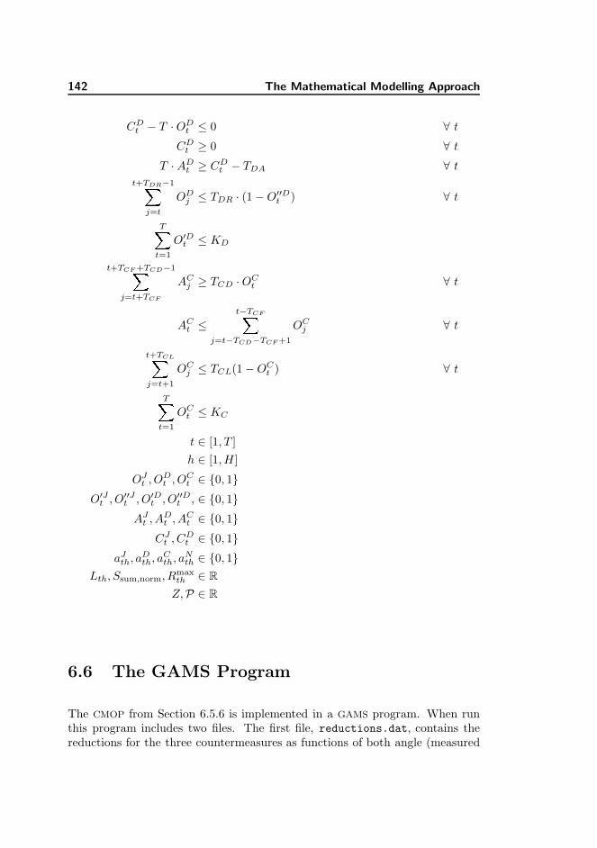
142 The Mathematical Modelling Approach
CDt − T ·OD
t ≤ 0 ∀ t
CDt ≥ 0 ∀ t
T · ADt ≥ CD
t − TDA ∀ t
t+TDR−1Xj=t
ODj ≤ TDR · (1−O′′D
t ) ∀ t
TXt=1
O′Dt ≤ KD
t+TCF +TCD−1Xj=t+TCF
ACj ≥ TCD ·O
Ct ∀ t
ACt ≤
t−TCFXj=t−TCD−TCF +1
OCj ∀ t
t+TCLXj=t+1
OCj ≤ TCL(1−OC
t ) ∀ t
TXt=1
OCt ≤ KC
t ∈ [1, T ]
h ∈ [1, H ]
OJt , OD
t , OCt ∈ {0, 1}
O′Jt , O′′J
t , O′Dt , O′′D
t , ∈ {0, 1}
AJt , AD
t , ACt ∈ {0, 1}
CJt , CD
t ∈ {0, 1}
aJth, aD
th, aCth, aN
th ∈ {0, 1}
Lth, Ssum,norm, Rmaxth ∈ R
Z,P ∈ R
6.6 The GAMS Program
The CMOP from Section 6.5.6 is implemented in a GAMS program. When runthis program includes two files. The first file, reductions.dat, contains thereductions for the three countermeasures as functions of both angle (measured
6.7 Testing 143
in degrees) and range (measured in percentage of maximum range). The secondfile describes the flight for which the optimal survivability is to be found. Itcontains the distances and angles to the threats in the scenario for every timestep in the timeframe. For each time step the lethalities for all threats are alsodescribed. The name of this file is given as an argument to GAMS when theprogram is run.
The GAMS program is included in Appendix D. Before the optimisation ofthe objective function is commenced the reductions of threat lethality for eachcountermeasure against every threat in each time step must be calculated. Thisis done by looking up the relevant values in the reductions.dat file included.Also the values of ρ∗th are calculated for all threats at every time step. Finallythe probability of every threat actually posing a threat is found for all timesteps. The model is solved by GAMS using a Mixed-Integer Problem solver inCPLEX.
When a solution is found the results are added to a file. These results describethe date and time of the run, the number of time steps in the time frame, theobjective value, the optimal survivability, the number of seconds used in findingthe solution, and finally the name of the input file. These results are used inparts of the tests described in Section 6.7.
6.7 Testing
The testing of the GAMS program is conducted in three steps: first a numberof test files are constructed to evaluate the time-related behaviour of the threecountermeasures. Second a number of flights are generated from two scenarios.This is done to find the time it takes for GAMS/CPLEX to find the optimalsolution depending on the number of time steps given in the flight. In the thirdand final step of the testing the optimal survivability to a number of differentscenarios are found.
The scenarios described by the test files used in the first step of testing themathematical model have very little resemblance with real world scenarios. Toeach time step described in these files fixed values for the distance and angleparameters are used. These values have been found to invoke responses fromeach of the countermeasures if no other constraints restrain them, and they areused to create a need for each countermeasure for a given period of time. Table6.2 shows the pairs of parameter values used in the files, and the reductionsgiven by each of the countermeasures using these values.
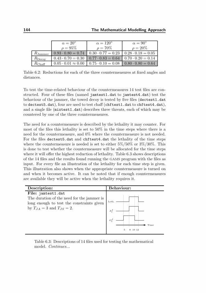
144 The Mathematical Modelling Approach
α = 20◦ α = 120◦ α = 90◦
ρ = 95% ρ = 70% ρ = 20%RJammer 0.93 · 0.80 = 0.74 0.30 · 0.77 = 0.23 0.28 · 0.18 = 0.05RDecoy 0.43 · 0.70 = 0.30 0.77 · 0.83 = 0.64 0.70 · 0.20 = 0.14RChaff 0.05 · 0.01 ≈ 0.00 0.75 · 0.10 = 0.08 0.80 · 0.80 = 0.64
Table 6.2: Reductions for each of the three countermeasures at fixed angles anddistances.
To test the time-related behaviour of the countermeasures 14 test files are con-structed. Four of these files (named jamtest1.dat to jamtest4.dat) test thebehaviour of the jammer, the towed decoy is tested by five files (dectest1.datto dectest5.dat), four are used to test chaff (chftest1.dat to chftest4.dat),and a single file (mixtest1.dat) describes three threats, each of which may becountered by one of the three countermeasures.
The need for a countermeasure is described by the lethality it may counter. Formost of the files this lethality is set to 50% in the time steps where there is aneed for the countermeasure, and 0% where the countermeasure is not needed.For the files dectest5.dat and chftest4.dat the lethality of the time stepswhere the countermeasure is needed is set to either 5%/50% or 3%/30%. Thisis done to test whether the countermeasure will be allocated for the time stepswhere it will offer the highest reduction of lethality. Table 6.3 shows descriptionsof the 14 files and the results found running the GAMS program with the files asinput. For every file an illustration of the lethality for each time step is given.This illustration also shows when the appropriate countermeasure is turned onand when it becomes active. It can be noted that if enough countermeasuresare available they will be active when the lethality requires it.
Description: Behaviour:File: jamtest1.dat
Leth.
AJt
OJt
Time
5 8 10 12
The duration of the need for the jammer islong enough to test the constraints givenby TJA = 3 and TJS = 2.
Table 6.3: Descriptions of 14 files used for testing the mathematicalmodel. Continues...
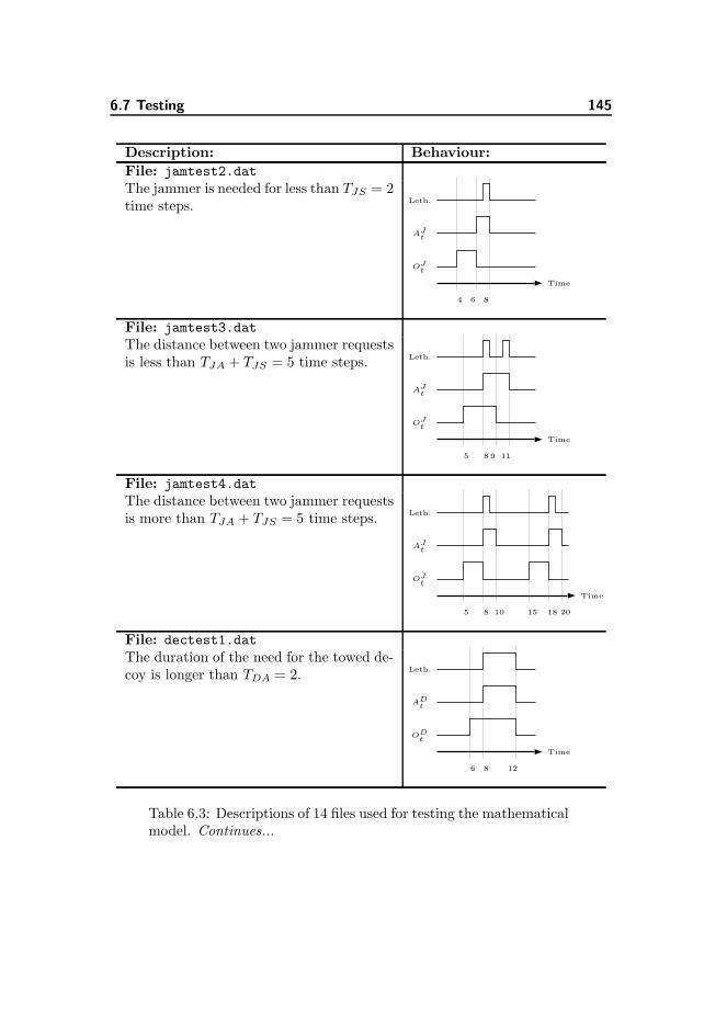
6.7 Testing 145
Description: Behaviour:
File: jamtest2.dat
Leth.
AJt
OJt
Time
4 6 8
The jammer is needed for less than TJS = 2time steps.
File: jamtest3.dat
Leth.
AJt
OJt
Time
5 8 9 11
The distance between two jammer requestsis less than TJA + TJS = 5 time steps.
File: jamtest4.dat
Leth.
AJt
OJt
Time
5 8 10 15 18 20
The distance between two jammer requestsis more than TJA + TJS = 5 time steps.
File: dectest1.dat
Leth.
ADt
ODt
Time
6 8 12
The duration of the need for the towed de-coy is longer than TDA = 2.
Table 6.3: Descriptions of 14 files used for testing the mathematicalmodel. Continues...
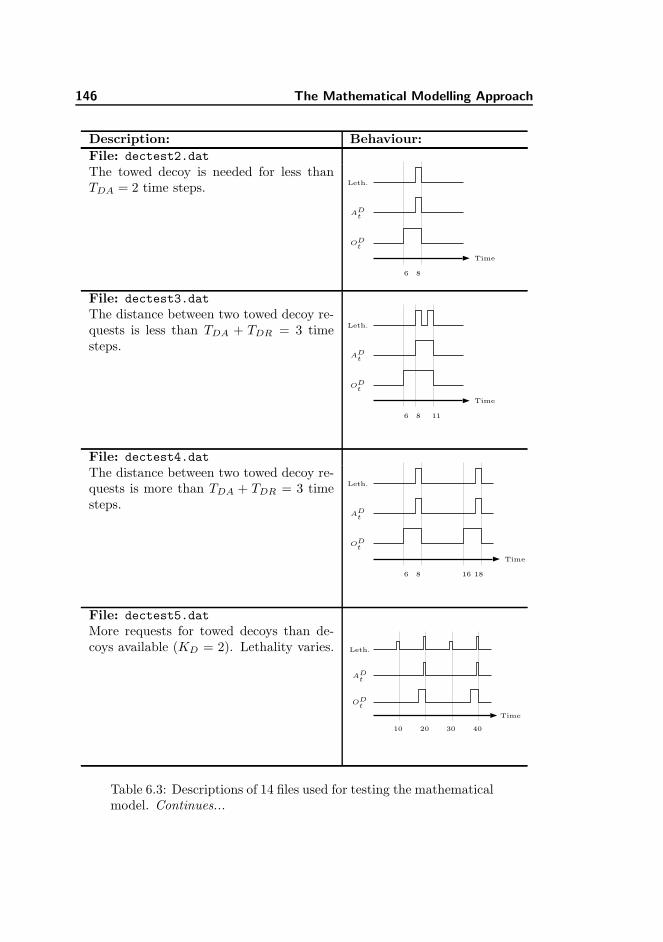
146 The Mathematical Modelling Approach
Description: Behaviour:
File: dectest2.dat
Leth.
ADt
ODt
Time
6 8
The towed decoy is needed for less thanTDA = 2 time steps.
File: dectest3.dat
Leth.
ADt
ODt
Time
6 8 11
The distance between two towed decoy re-quests is less than TDA + TDR = 3 timesteps.
File: dectest4.dat
Leth.
ADt
ODt
Time
6 8 16 18
The distance between two towed decoy re-quests is more than TDA + TDR = 3 timesteps.
File: dectest5.dat
Leth.
ADt
ODt
Time
10 20 30 40
More requests for towed decoys than de-coys available (KD = 2). Lethality varies.
Table 6.3: Descriptions of 14 files used for testing the mathematicalmodel. Continues...
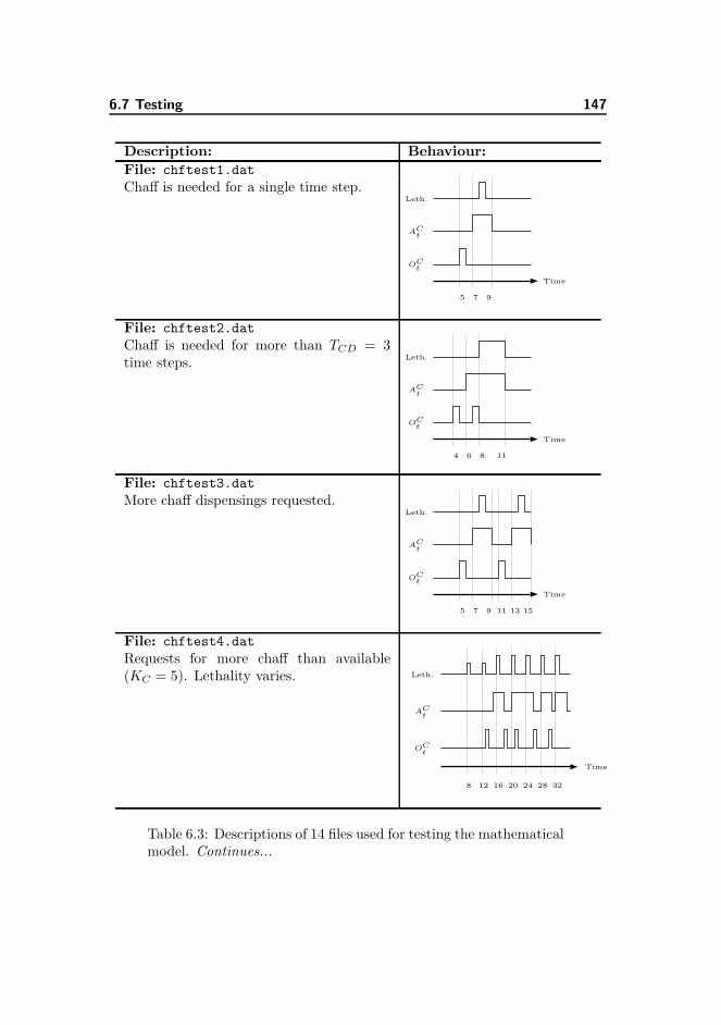
6.7 Testing 147
Description: Behaviour:
File: chftest1.dat
Leth.
ACt
OCt
Time
5 7 9
Chaff is needed for a single time step.
File: chftest2.dat
Leth.
ACt
OCt
Time
4 6 8 11
Chaff is needed for more than TCD = 3time steps.
File: chftest3.dat
Leth.
ACt
OCt
Time
5 7 9 11 13 15
More chaff dispensings requested.
File: chftest4.dat
Leth.
ACt
OCt
Time
8 12 16 20 24 28 32
Requests for more chaff than available(KC = 5). Lethality varies.
Table 6.3: Descriptions of 14 files used for testing the mathematicalmodel. Continues...
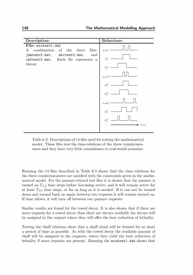
148 The Mathematical Modelling Approach
Description: Behaviour:
File: mixtest1.datLeth1.
AJt
OJt
Leth2.
ADt
ODt
Leth3.
ACt
OCt
Time
A combination of the three files:jamtest3.dat, dectest3.dat, andchftest3.dat. Each file represents athreat.
Table 6.3: Descriptions of 14 files used for testing the mathematicalmodel. These files test the time-relations of the three countermea-sures and they have very little resemblance to real-world scenarios.
Running the 14 files described in Table 6.3 shows that the time relations forthe three countermeasures are satisfied with the constraints given in the mathe-matical model. For the jammer-related test files it is shown that the jammer isturned on TJA time steps before becoming active, and it will remain active forat least TJS time steps, or for as long as it is needed. If it can not be turneddown and turned back on again between two requests it will remain turned on.If time allows, it will turn off between two jammer requests.
Similar results are found for the towed decoy. It is also shown that if there aremore requests for a towed decoy than there are decoys available the decoys willbe assigned to the request where they will offer the best reduction of lethality.
Testing the chaff relations show that a chaff cloud will be formed for as shorta period of time as possible. As with the towed decoy the available amount ofchaff will be assigned to the requests, where they yield the best reduction oflethality if more requests are present. Running the mixtest1.dat shows that
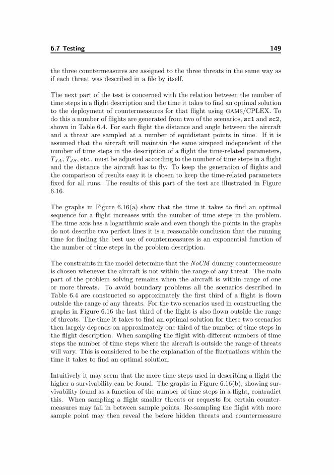
6.7 Testing 149
the three countermeasures are assigned to the three threats in the same way asif each threat was described in a file by itself.
The next part of the test is concerned with the relation between the number oftime steps in a flight description and the time it takes to find an optimal solutionto the deployment of countermeasures for that flight using GAMS/CPLEX. Todo this a number of flights are generated from two of the scenarios, sc1 and sc2,shown in Table 6.4. For each flight the distance and angle between the aircraftand a threat are sampled at a number of equidistant points in time. If it isassumed that the aircraft will maintain the same airspeed independent of thenumber of time steps in the description of a flight the time-related parameters,TJA, TJS , etc., must be adjusted according to the number of time steps in a flightand the distance the aircraft has to fly. To keep the generation of flights andthe comparison of results easy it is chosen to keep the time-related parametersfixed for all runs. The results of this part of the test are illustrated in Figure6.16.
The graphs in Figure 6.16(a) show that the time it takes to find an optimalsequence for a flight increases with the number of time steps in the problem.The time axis has a logarithmic scale and even though the points in the graphsdo not describe two perfect lines it is a reasonable conclusion that the runningtime for finding the best use of countermeasures is an exponential function ofthe number of time steps in the problem description.
The constraints in the model determine that the NoCM dummy countermeasureis chosen whenever the aircraft is not within the range of any threat. The mainpart of the problem solving remains when the aircraft is within range of oneor more threats. To avoid boundary problems all the scenarios described inTable 6.4 are constructed so approximately the first third of a flight is flownoutside the range of any threats. For the two scenarios used in constructing thegraphs in Figure 6.16 the last third of the flight is also flown outside the rangeof threats. The time it takes to find an optimal solution for these two scenariosthen largely depends on approximately one third of the number of time steps inthe flight description. When sampling the flight with different numbers of timesteps the number of time steps where the aircraft is outside the range of threatswill vary. This is considered to be the explanation of the fluctuations within thetime it takes to find an optimal solution.
Intuitively it may seem that the more time steps used in describing a flight thehigher a survivability can be found. The graphs in Figure 6.16(b), showing sur-vivability found as a function of the number of time steps in a flight, contradictthis. When sampling a flight smaller threats or requests for certain counter-measures may fall in between sample points. Re-sampling the flight with moresample point may then reveal the before hidden threats and countermeasure
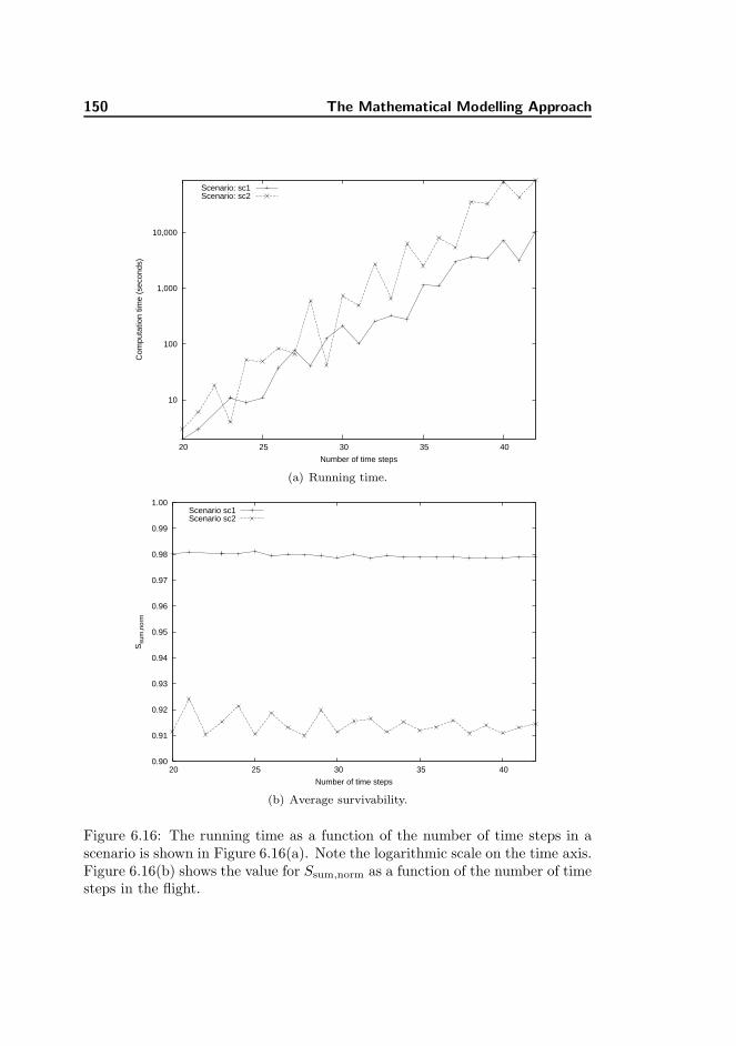
150 The Mathematical Modelling Approach
10,000
1,000
100
10
20 25 30 35 40
Com
puta
tion
time
(sec
onds
)
Number of time steps
Scenario: sc1Scenario: sc2
(a) Running time.
1.00
0.99
0.98
0.97
0.96
0.95
0.94
0.93
0.92
0.91
0.90 20 25 30 35 40
Ssu
m,n
orm
Number of time steps
Scenario sc1Scenario sc2
(b) Average survivability.
Figure 6.16: The running time as a function of the number of time steps in ascenario is shown in Figure 6.16(a). Note the logarithmic scale on the time axis.Figure 6.16(b) shows the value for Ssum,norm as a function of the number of timesteps in the flight.
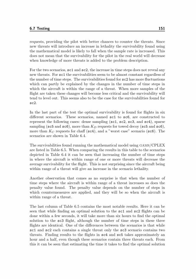
6.7 Testing 151
requests, providing the pilot with better chances to counter the threats. Sincenew threats will introduce an increase in lethality the survivability found usingthe mathematical model is likely to fall when the sample rate is increased. Thisdoes not mean that the survivability for the pilot in the real world will decreasewhen knowledge of more threats is added to the problem description.
For the two scenarios, sc1 and sc2, the increase in time steps does not reveal anynew threats. For sc1 the survivabilities seem to be almost constant regardless ofthe number of time steps. The survivabilities found for sc2 has more fluctuationswhich can partly be explained by the changes in the number of time steps inwhich the aircraft is within the range of a threat. When more samples of theflight are taken these changes will become less critical and the survivability willtend to level out. This seems also to be the case for the survivabilities found forsc2.
In the last part of the test the optimal survivability is found for flights in sixdifferent scenarios. These scenarios, named sc1 to sc6, are constructed torepresent the following cases: dense sampling (sc1, sc2, sc3, and sc4), sparsesampling (sc5 and sc6), more than KD requests for towed decoy (sc5 and sc6),more than KC requests for chaff (sc4), and a ”worst case” scenario (sc6). Thescenarios are shown in Table 6.4.
The survivabilities found running the mathematical model using GAMS/CPLEXare listed in Table 6.5. When comparing the results in this table to the scenariosdepicted in Table 6.4 it can be seen that increasing the number of time stepsin where the aircraft is within range of one or more threats will decrease theaverage survivability for the flight. This is not surprising since the aircraft beingwithin range of a threat will give an increase in the scenario lethality.
Another observation that comes as no surprise is that when the number oftime steps where the aircraft is within range of a threat increases so does thepenalty value found. The penalty value depends on the number of steps inwhich countermeasures are applied, and they will be so when the aircraft iswithin range of a threat.
The last column of Table 6.5 contains the most notable results. Here it can beseen that while finding an optimal solution to the sc1 and sc2 flights can bedone within a few seconds, it will take more than six hours to find the optimalsolution to the sc3 flight, although the number of time steps in these threeflights are identical. One of the differences between the scenarios is that whilesc1 and sc2 each contains a single threat only the sc3 scenario contains twothreats. Finding results to the flights in sc4 and sc5 takes approximately anhour and a half, even though these scenarios contain three threats each. Fromthis it can be seen that estimating the time it takes to find the optimal solution
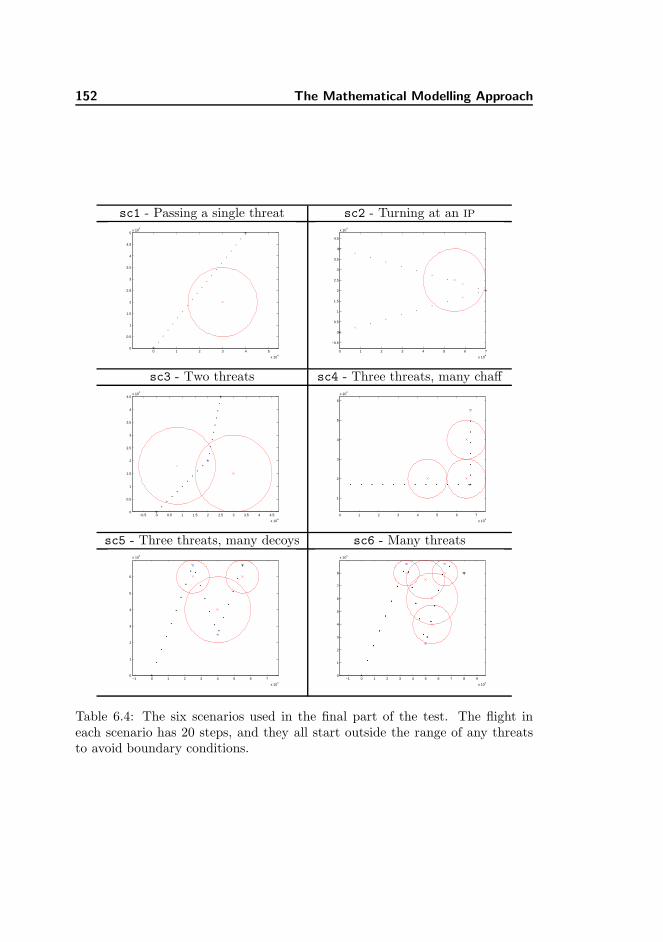
152 The Mathematical Modelling Approach
sc1 - Passing a single threat sc2 - Turning at an IP
0 1 2 3 4 5
x 104
0
0.5
1
1.5
2
2.5
3
3.5
4
4.5
5x 10
4
0 1 2 3 4 5 6 7
x 104
−0.5
0
0.5
1
1.5
2
2.5
3
3.5
4
4.5
x 104
sc3 - Two threats sc4 - Three threats, many chaff
−0.5 0 0.5 1 1.5 2 2.5 3 3.5 4 4.5
x 104
0
0.5
1
1.5
2
2.5
3
3.5
4
4.5x 10
4
0 1 2 3 4 5 6 7
x 104
1
2
3
4
5
6
x 104
sc5 - Three threats, many decoys sc6 - Many threats
−1 0 1 2 3 4 5 6 7
x 104
0
1
2
3
4
5
6
x 104
−1 0 1 2 3 4 5 6 7 8 9
x 104
0
1
2
3
4
5
6
7
8
x 104
Table 6.4: The six scenarios used in the final part of the test. The flight ineach scenario has 20 steps, and they all start outside the range of any threatsto avoid boundary conditions.
6.8 Discussion 153
Scenario: Ssum,norm: Penalty: Running time:sc1 0.98211 0.0016 2sc2 0.91419 0.0027 6sc3 0.91214 0.0037 22326sc4 0.83773 0.0065 5858sc5 0.83773 0.0065 5708sc6 - - 37916
Table 6.5: Results of solving flights for six different scenarios. Running timeis measured in seconds. The process of finding a solution to the sc6 flight isterminated by the solver, and no solution is found.
to a flight is not trivial, as it apparently depends on more than the number oftime steps in the flight, the number of time steps within range of a threat, andthe number of threats in the flight scenario.
6.8 Discussion
In both the Prolog approach (Chapter 4) and the BN approach (Chapter 5) thefocus was on finding the appropriate use of countermeasures at each point intime. With the approach described in this chapter it is assumed that the processof finding the best countermeasures to use at any given time can be reduced toa simple table lookup. In a real-world implementation of this approach the bestcountermeasure to apply at any time may be found by consulting e.g. a Prologprogram or a BN.
If a countermeasure is to be active during the first few time steps of the timeframe, solving the model will make the countermeasure being turned on beforethe start of the time frame. As this is not considered a correct answer, the flightsare constructed in such a way that no threats are imminent in the beginningof the time frame. Doing this the model does not need to be concerned withboundary issues.
The aircraft can be protected by a countermeasure at any time. If neither toweddecoys nor chaff are available an active jammer may always offer some reductionof lethality. This is only prevented if the jammer can not be turned on sometime ahead. This happens only if the jammer is still active from a previousdeployment interval. Extending this interval to fulfil the new requirements willsolve the problem. Here boundary issues are neglected and it is assumed thatthe jammer can be turned on in any time step, even if this time step lies beforethe start of the time frame.
154 The Mathematical Modelling Approach
Compared to dispensing chaff the fiscal cost of deploying and releasing a toweddecoy is very high. Even if the towed decoy offers only a slightly better pro-tection than chaff, solving the model described in this chapter will select thetowed decoy over chaff, not taking the cost of this into account. If the cost wasincorporated in the objective function, such that chaff dispensing were preferredeven if this results in a slightly worse reduction of lethality than using a toweddecoy, the solutions found might be closer to what a fighter pilot will choosewhen in the same situation. Determining the allowable decrease in survivabilityto save the deployment of towed decoys is considered outside the scope of thiswork.
A large part of the work on the mathematical model is spend on determining theconstraints describing the relations between the time steps in where a counter-measure is turned on and the time steps in where it is active. The survivabilityof the fighter aircraft depends only on when countermeasures are active, andnot on when they are turned on. It may therefore be beneficial to leave the vari-ables describing the latter out of the model. The period in which the jammer isturned on without being active sets a limit to how close jammer deployment in-tervals can be. It is assumed that this can be described using fewer and simplerconstraints than the ones describing relations between the OJ
t and AJt variables.
For the towed decoy the time between deployment intervals is set by the sumof the time it takes to settle after a decoy has been released, and the time ittakes to unreel a new decoy. Here the need of a variable describing when adecoy is deployed is not evident either. Since chaff can be dispensed while thecloud from a previous dispensing is still formed, it may be that describing thetime-relations for chaff can not be done by a single variable only. Still, omittinga large number of variables and constraints for the jammer and the towed decoyis likely to decrease the total computation time for finding an optimal solution.
According to Section 6.4.3 a total of 1500 time steps may be needed for de-scribing a mission with a duration of up to five minutes, if the resolution of thedescription is set to five time steps per second. While this resolution may seemadequate, a coarser resolution can be acceptable. For the six scenarios used fortesting the mathematical model, the number of time steps was chosen withoutconsidering the length of the flight and the time it will take to fly this. Theflight in sc1 is one of the shortest of the six flights. From start point to targetthis flight is approximately 64 km. With a speed of Mach 2 (2,124 km/h) afighter aircraft will fly this distance in little more than 100 seconds. Decreasingthe proposed resolution by a factor of 10, the time steps are set two secondsapart. With this the description of the sc1 flight will require approximately 50time steps; more than twice the number of time steps used in the tests describedin this chapter. Descriptions of the other flights, with the sc3 flight as an ex-ception, will require even more time steps. Since GAMS/CPLEX in the defaultconfiguration can not be expected to solve larger problems within a reasonably
6.9 Conclusion 155
time, it may be necessary to use other configurations, or to split the problemsinto subproblems, that may be solved separately.
6.9 Conclusion
This chapter shows that for a simple model of a scenario containing ground basedradar threats a survivability measure for fighter aircraft can be described. Fromthis a mathematical model can be formulated to describe how a set of coun-termeasures influence the survivability. Both the survivability and the counter-measure influence are based upon the use of RF based threats only. Broaderdescriptions, e.g. including both IR and RF based threats, are likely to be sig-nificantly more complicated than the survivability measure and countermeasureinfluence described here.
A large part of the mathematical model describes the time relations of coun-termeasures. If other countermeasures are to be added to the model it is likelythat some of the constraints constructed can be adaptable to work for thesecountermeasures as well. As described in Section 6.8 some of these constraintsmay not be necessary.
The use of GAMS/CPLEX described in this work will not allow for solutionsto larger problems to be found within a reasonably time. Even for small andsimple scenarios, as the six test scenarios described in this chapter, finding asolution takes a very long time. Using non-uniform time steps and weighting asdescribed in Section 6.4.3 may relieve this issue. If the solving method can itselfbe optimized, so that problems in a real-world scenario can be solved in real-time, the success of this approach still relates to the availability of knowledgeabout the scenario. If the system has no knowledge about a threat prior toentering its lethal range, an optimal solution for the entire mission can not beguaranteed.
Even if solving the mathematical model can never meet the real-time require-ment, the model may still have a number of useful applications. If a real-worldscenario has a fixed number of threats reported by intelligence, a solution foundpre-mission can be applied. A number of standard scenarios may also be de-fined, and the optimal sequence of applying countermeasures in these can beapplied when needed. Chapter 7 describes the use of metaheuristics to findgood solutions to the CMOP. Optimal solutions found using GAMS/CPLEX canbe used in improving the performance of such a metaheuristic.

156 The Mathematical Modelling Approach

Chapter 7
The Metaheuristics Approach
A heuristic is an algorithm that uses some knowledge about a concrete problemin the process of finding a solution to it. Usually it can not be guaranteed that aheuristic finds the best solution to the problem, or even that the solution foundis feasible. A metaheuristic is an algorithm framework that describes how to findsolutions without being concerned with problem-specific considerations. Theseconsiderations must, naturally, be made when implementing a metaheuristic forsolving a given type of problems. As a tailored metaheuristic is a heuristic thefeasibility and optimality of the solutions found can not always be guaranteed.Metaheuristics are often applied for problems within the field of combinato-rial optimisation, where they usually provide good, but not necessarily optimal,solutions. They have proven successful when no exact method for finding asolution is known, or when only a limited amount of computing time is avail-able. Throughout this text the word ”algorithm” refers to the metaheuristic itdescribes.
The choice of the metaheuristic to use in solving a problem, and setting up pa-rameters for this, depends on several factors. These factors include the type ofproblem to solve, how close to optimum the solutions must be, and how fast themetaheuristic has to provide solutions. This chapter gives a general introduc-tion to metaheuristics, some details on the Simulated Annealing metaheuristic,and comments on an implementation of this algorithm. Readers familiar withmetaheuristics in general, and the Simulated Annealing specifically, may skip to
158 The Metaheuristics Approach
Section 7.4, where an implementation of the Simulated Annealing metaheuris-tic for solving the Countermeasure Optimisation Problem (CMOP) derived inChapter 6 is described.
7.1 Motivation
With the CMOP the goal is to find the deployment scheme that provides the bestsurvivability for a fighter aircraft during a mission. It is possible to calculate thetotal survivability for all possible instances of the deployment scheme, and thenselect the deployment scheme yielding the highest survivability. Unfortunately,this approach is infeasible for problems with more than a minimum number oftime steps in the deployment scheme since the generation and evaluation of allthe schemes will simply take too long.
In Chapter 6 solutions to the CMOP is found using mathematical programming.Using GAMS/CPLEX shows that an optimal solution can be found to someproblems, and even though this can be done very fast compared to the timeit takes to generate all possible deployment schemes, the time it takes to findan optimal solution is still too long. Therefore a solution is sought using ametaheuristic.
The fact that a metaheuristic can not be guaranteed to find an optimal solutionis not considered important for finding a solution to the CMOP. The descriptionof a battlefield scenario will often be so deficient that there is no way of decidingwhether the exact optimal solution found is in reality superior to any other goodsolution. To the pilot any solution that significantly increases the chances ofsurvival may be considered a good solution.
7.2 Metaheuristics
The search space of a problem is the set of all possible solutions to that problem.For a combinatorial optimisation problem the search space will consist of allcombinations of values for the variables included in the problem. A problemsuitable for a metaheuristic will usually have a search space that is too large tobe searched completely. A metaheuristic will search parts of the search space inthe pursuit of the optimal solution.
In general a metaheuristic first finds an initial solution, and in iterations bettersolutions are found, until it comes to a stop. In every iteration the current best
7.2 Metaheuristics 159
solution is known as the incumbent, and the solution being the incumbent atthe end of the run is returned by the metaheuristic. In the search for improvedsolutions a number of candidate solutions are compared to the incumbent. Newcandidates are chosen from the neighbourhood of the incumbent. These candi-dates are also known as neighbours.
The metaheuristic runs for a number of iterations, and the incumbent may bereplaced by a better solution in each of the iterations. The number of iterationsis determined by one or more stopping criteria. The run may be stopped if thetotal number of iterations exceeds some preset limit, or if the incumbent hasnot been replaced for a fixed number of iterations. Also, reaching a maximumamount of computation time may be used as a stopping criterion.
In this work three metaheuristics are investigated: Local Search, Steepest As-cent, and Simulated Annealing. The three metaheuristics have been chosen fortheir simplicity, which makes them easy to implement. Steepest Ascent and Sim-ulated Annealing can both be considered special cases of a general Local Searchmetaheuristic, and this makes the comparison of the three even easier, sincethe comparison can be done using the same program with only minor changes.Other metaheuristics such as Genetic Algorithms or Tabu Search may providesolutions of a quality equal to or better than those found using Local Search,Steepest Ascent, or Simulated Annealing. The intention of the work describedin this chapter is to evaluate the use of metaheuristics for solving the CMOP. Itis estimated that this can be done by implementing the three countermeasuresmentioned, and therefore no other metaheuristics have been chosen.
7.2.1 Local Search
In the Local Search metaheuristic candidates from the neighbourhood of theincumbent are selected at random. If a candidate solution is proven better thanthe incumbent it becomes the new incumbent. The algorithm continues untilno improving neighbour can be found, or until a maximum number of iterationshave been run. The Local Search metaheuristic for maximising the objectivefunction is given in Algorithm 1. Here f(s) is the objective function that returnsa value for the solution s.
This metaheuristic will search for the optimum local to the initial solution. Ifthis optimum is reached, i.e. there is no neighbouring solutions that will improvethe solution, the metaheuristic will stop. Applying the algorithm a number oftimes on the same problem may find a number of local optima from which thebest optimum found can be selected.
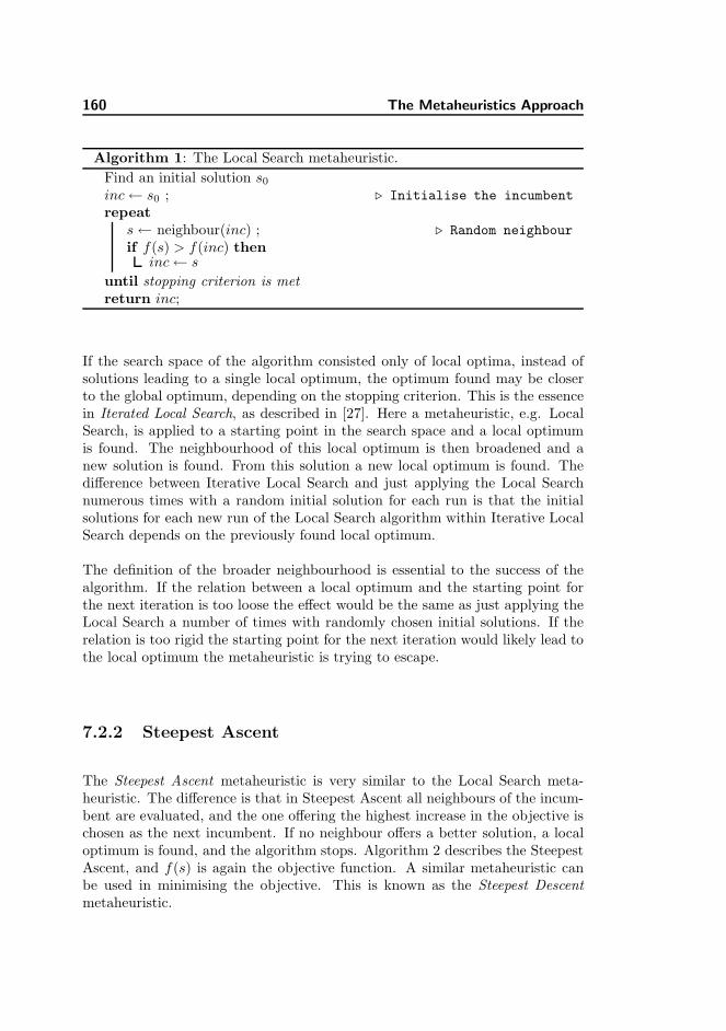
160 The Metaheuristics Approach
Algorithm 1: The Local Search metaheuristic.
Find an initial solution s0
inc← s0 ; . Initialise the incumbent
repeats← neighbour(inc) ; . Random neighbour
if f(s) > f(inc) theninc← s
until stopping criterion is metreturn inc;
If the search space of the algorithm consisted only of local optima, instead ofsolutions leading to a single local optimum, the optimum found may be closerto the global optimum, depending on the stopping criterion. This is the essencein Iterated Local Search, as described in [27]. Here a metaheuristic, e.g. LocalSearch, is applied to a starting point in the search space and a local optimumis found. The neighbourhood of this local optimum is then broadened and anew solution is found. From this solution a new local optimum is found. Thedifference between Iterative Local Search and just applying the Local Searchnumerous times with a random initial solution for each run is that the initialsolutions for each new run of the Local Search algorithm within Iterative LocalSearch depends on the previously found local optimum.
The definition of the broader neighbourhood is essential to the success of thealgorithm. If the relation between a local optimum and the starting point forthe next iteration is too loose the effect would be the same as just applying theLocal Search a number of times with randomly chosen initial solutions. If therelation is too rigid the starting point for the next iteration would likely lead tothe local optimum the metaheuristic is trying to escape.
7.2.2 Steepest Ascent
The Steepest Ascent metaheuristic is very similar to the Local Search meta-heuristic. The difference is that in Steepest Ascent all neighbours of the incum-bent are evaluated, and the one offering the highest increase in the objective ischosen as the next incumbent. If no neighbour offers a better solution, a localoptimum is found, and the algorithm stops. Algorithm 2 describes the SteepestAscent, and f(s) is again the objective function. A similar metaheuristic canbe used in minimising the objective. This is known as the Steepest Descentmetaheuristic.
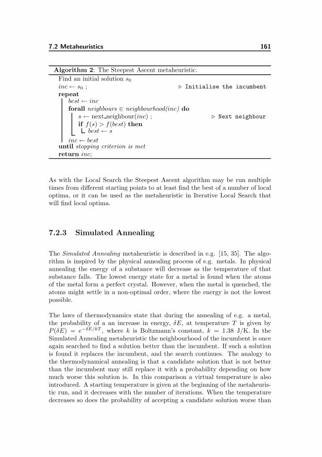
7.2 Metaheuristics 161
Algorithm 2: The Steepest Ascent metaheuristic.
Find an initial solution s0
inc← s0 ; . Initialise the incumbent
repeatbest← incforall neighbours ∈ neighbourhood(inc) do
s← next neighbour(inc) ; . Next neighbour
if f(s) > f(best) thenbest← s
inc← bestuntil stopping criterion is metreturn inc;
As with the Local Search the Steepest Ascent algorithm may be run multipletimes from different starting points to at least find the best of a number of localoptima, or it can be used as the metaheuristic in Iterative Local Search thatwill find local optima.
7.2.3 Simulated Annealing
The Simulated Annealing metaheuristic is described in e.g. [15, 35]. The algo-rithm is inspired by the physical annealing process of e.g. metals. In physicalannealing the energy of a substance will decrease as the temperature of thatsubstance falls. The lowest energy state for a metal is found when the atomsof the metal form a perfect crystal. However, when the metal is quenched, theatoms might settle in a non-optimal order, where the energy is not the lowestpossible.
The laws of thermodynamics state that during the annealing of e.g. a metal,the probability of a an increase in energy, δE, at temperature T is given byP (δE) = e−δE/kT , where k is Boltzmann’s constant, k = 1.38 J/K. In theSimulated Annealing metaheuristic the neighbourhood of the incumbent is onceagain searched to find a solution better than the incumbent. If such a solutionis found it replaces the incumbent, and the search continues. The analogy tothe thermodynamical annealing is that a candidate solution that is not betterthan the incumbent may still replace it with a probability depending on howmuch worse this solution is. In this comparison a virtual temperature is alsointroduced. A starting temperature is given at the beginning of the metaheuris-tic run, and it decreases with the number of iterations. When the temperaturedecreases so does the probability of accepting a candidate solution worse than
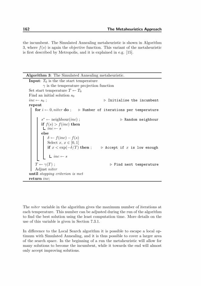
162 The Metaheuristics Approach
the incumbent. The Simulated Annealing metaheuristic is shown in Algorithm3, where f(s) is again the objective function. This variant of the metaheuristicis first described by Metropolis, and it is explained in e.g. [15].
Algorithm 3: The Simulated Annealing metaheuristic.
Input: T0 is the the start temperatureγ is the temperature projection function
Set start temperature T ← T0
Find an initial solution s0
inc← s0 ; . Initialise the incumbent
repeatfor i← 0, niter do ; . Number of iterations per temperature
s∗ ← neighbour(inc) ; . Random neighbour
if f(s) > f(inc) theninc← s
elseδ ← f(inc)− f(s)Select x, x ∈ [0, 1]if x < exp(−δ/T ) then ; . Accept if x is low enough
inc← s
T ← γ(T ) ; . Find next temperature
Adjust niteruntil stopping criterion is metreturn inc;
The niter variable in the algorithm gives the maximum number of iterations ateach temperature. This number can be adjusted during the run of the algorithmto find the best solution using the least computation time. More details on theuse of this variable is given in Section 7.3.1.
In difference to the Local Search algorithm it is possible to escape a local op-timum with Simulated Annealing, and it is thus possible to cover a larger areaof the search space. In the beginning of a run the metaheuristic will allow formany solutions to become the incumbent, while it towards the end will almostonly accept improving solutions.
7.2 Metaheuristics 163
7.2.4 Choosing a Metaheuristic
In implementing a metaheuristic most of the work is spend in defining con-straints and variable relations, determining what constitutes the neighbourhoodof a given solution, and how a neighbour is selected at random. Since these con-siderations are almost identical for the three metaheuristics described in thissection, they alone do not suggest which metaheuristic to choose. In solving theCMOP the proper metaheuristic should provide a good solution within a veryshort time span. For every iteration of the Steepest Ascent metaheuristic itneeds to generate and evaluate every neighbour solution. Since every solutionmay have a large neighbourhood, the Steepest Ascent algorithm may have per-formed a few iterations only, before it is stopped by a given maximum runningtime, and the best solution found may not differ substantially from the initialsolution. The Local Search algorithm may perform a little faster, since it gen-erates only the amount of neighbour solutions necessary for it to improve itsbest solution. The drawback of the Local Search is that it may spend most ofits time on finding the optimum local to the initial solution, without any searchfor a better solution. The Simulated Annealing mends this, as it is designed toescape local optima at the beginning of a run. For large neighbourhoods it per-forms faster than the Steepest Ascent, and while it is deemed to be slower thanthe Local Search, it may escape local optima, and it thus have the possibility offinding better solutions.
Figure 7.1 shows the progress of improving the survivability for each of themetaheuristics. It can be seen that Local Search will reach a steady state aftera relatively short time. The Steepest Ascent keeps improving its solution andno steady state is reached within the time given. In the first part of the timegiven, the survivability found by the Simulated Annealing fluctuates. It findsa steady state later than the Local Search, and the survivability found here ishigher than that of either of the other metaheuristics.
According to [15] Simulated Annealing offers the best results on uniform data,i.e. data where very few clusters are present in the search space. This is incontradiction to a typical solution for the CMOP where each countermeasurewill be active only within a number of deployment intervals, and these intervalsoften occur only when the aircraft is close to a threat. Both the deploymentintervals and the presence of a threat can be considered as clusters in the solutionspace, and therefore Simulated Annealing may not show the best performancesolving the CMOP.
In the literature on Simulated Annealing [15] the algorithm has been shown togive good results for most of the problems it has been applied to, albeit morespecific heuristics usually perform better. If the problem at hand has too many
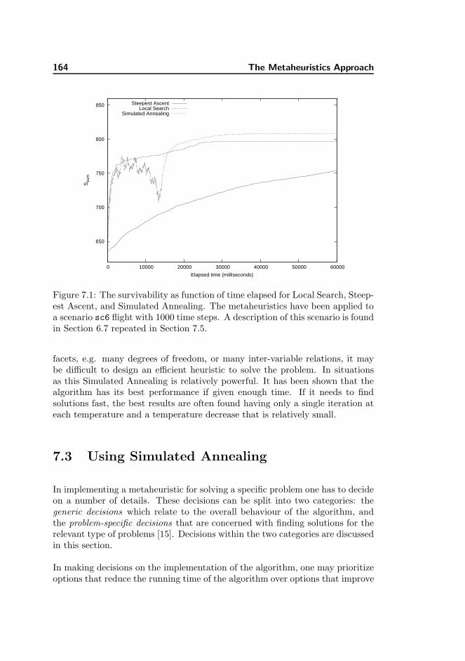
164 The Metaheuristics Approach
650
700
750
800
850
0 10000 20000 30000 40000 50000 60000
Ssu
m
Elapsed time (milliseconds)
Steepest AscentLocal Search
Simulated Annealing
Figure 7.1: The survivability as function of time elapsed for Local Search, Steep-est Ascent, and Simulated Annealing. The metaheuristics have been applied toa scenario sc6 flight with 1000 time steps. A description of this scenario is foundin Section 6.7 repeated in Section 7.5.
facets, e.g. many degrees of freedom, or many inter-variable relations, it maybe difficult to design an efficient heuristic to solve the problem. In situationsas this Simulated Annealing is relatively powerful. It has been shown that thealgorithm has its best performance if given enough time. If it needs to findsolutions fast, the best results are often found having only a single iteration ateach temperature and a temperature decrease that is relatively small.
7.3 Using Simulated Annealing
In implementing a metaheuristic for solving a specific problem one has to decideon a number of details. These decisions can be split into two categories: thegeneric decisions which relate to the overall behaviour of the algorithm, andthe problem-specific decisions that are concerned with finding solutions for therelevant type of problems [15]. Decisions within the two categories are discussedin this section.
In making decisions on the implementation of the algorithm, one may prioritizeoptions that reduce the running time of the algorithm over options that improve
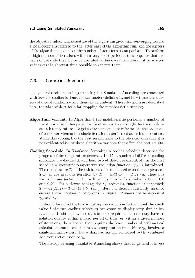
7.3 Using Simulated Annealing 165
the objective value. The structure of the algorithm gives that converging towarda local optima is referred to the latter part of the algorithm run, and the successof the algorithm depends on the number of iterations it can perform. To performa high number of iterations within a very short period of time requires that theparts of the code that are to be executed within every iteration must be writtenso it takes the shortest time possible to execute them.
7.3.1 Generic Decisions
The general decisions in implementing the Simulated Annealing are concernedwith how the cooling is done, the parameters defining it, and how these affect theacceptance of solutions worse than the incumbent. These decisions are describedhere, together with criteria for stopping the metaheuristic running.
Algorithm Variant. In Algorithm 3 the metaheuristic performs a number ofiterations at each temperature. In other variants a single iteration is doneat each temperature. To get to the same amount of iterations the cooling isoften slower when only a single iteration is performed at each temperature.While this cooling has the best resemblance to the physical annealing it isnot evident which of these algorithm variants that offers the best results.
Cooling Schedule. In Simulated Annealing a cooling schedule describes theprogress of the temperature decrease. In [15] a number of different coolingschedules are discussed, and here two of these are described. In the firstschedule a geometric temperature reduction function, γG, is introduced.The temperature Ti in the i’th iteration is calculated from the temperatureTi−1 at the previous iteration by Ti = γG(Ti−1) = Ti−1 · a. Here a isthe reduction factor, and it will usually have a fixed value between 0.8and 0.99. For a slower cooling the γS reduction function is suggested:Ti = γS(Ti−1) = Ti−1/(1 + b · Ti−1). Here b is chosen sufficiently small toensure a slow cooling. The graphs in Figure 7.2 shows the behaviour ofγG and γS .
It should be noted that in adjusting the reduction factor a and the smallvalue b the two cooling schedules can come to display very similar be-haviour. If this behaviour satisfies the requirements one may have tosolution quality within a fixed period of time, or within a given numberof iterations, the schedule that requires the least number of arithmeticalcalculations can be selected to save computation time. Since γG involves asingle multiplication it has a slight advantage compared to the combinedaddition and division of γS .
The history of using Simulated Annealing shows that in general it is less
166 The Metaheuristics Approach
0
10
20
30
40
50
60
70
80
90
100
0 10 20 30 40 50 60 70 80 90 100
Tem
pera
ture
Time step
Geometrical temperature reductionSlow temperature reduction
Figure 7.2: The behaviour of two different cooling schedules.
important how the cooling is done, and more important for how long thealgorithm is allowed to search for improving solutions. The best parametersettings for the cooling schedule chosen are problem dependent, and theymust be found in trials with representative problems [15].
The higher the reduction factor, the faster the metaheuristic will tend todismiss solutions worse than the incumbent. This means that the meta-heuristic will sooner focus on finding the local optimum. The reductionfactor must be chosen in such a way that a sufficiently large amount oflocal optima can be explored.
The Metropolis formulation of the algorithm suggests that a number ofiterations are performed at each temperature, before the temperature isreduced. The number of iterations can be fixed, or it may vary accordingto the temperature so that more neighbours are tested at lower tempera-tures where the probability of finding an improving solution is at its lowest.Varying the number of iterations can e.g. be done using geometrical orarithmetical projections, or by using a feed-back function. In finding thenumber geometrically the new number of iterations, i′ is found by multi-plying the old number of iterations, i, with a number b: i′ = i · b, b > 1. Inthe arithmetical approach the new number of iterations is found adding afixed number to the old number of iterations: i′ = i + b. If the number ofiterations is to be found using feed-back, a limit can be set to the numberof iterations where no improvement is done. Doing this the number ofiterations at each temperature adapts to the solutions found. The num-
7.3 Using Simulated Annealing 167
ber of idle iterations allowed may itself depend on the temperature; thusadding to the complexity of finding the best parameter settings for thealgorithm.
Start Temperature. The behaviour of the algorithm during the start of therun depends highly on the start temperature given. The higher this tem-perature is the more solutions will get accepted during the start phase. Ifit is too high each new solution will be accepted, and the iterations of themetaheuristic will behave like a number of random solutions picked fromthe search space. If the start temperature is too low the ability to escapelocal optimum by accepting non-improving solutions will be decreased.
End Temperature. Choosing the end temperature is one way of selecting astopping criterion. The faster the temperature reaches the end temper-ature the faster the algorithm is halted. On the other hand, if the endtemperature is set too low, the algorithm may have many iterations at theend where there is no improvement in the solutions found.
Acceptance Probability. The difference between the incumbent and a can-didate solution is used in determining if the candidate can be accepted.Letting the Boltzman probability, P (δE) = e−δE/kT , decide whether asolution worse than the incumbent can be accepted as the new incumbentwill keep the analogy to the physical annealing intact. While this proba-bility may work in an implementation of Simulated Annealing, it may notbe the best choice of acceptance probability.
Some implementations have shown that evaluating a new solution usingthe exponential function may use as much as one third of the total exe-cution time [15]. Therefore it may be appropriate to find an acceptanceprobability not using the exponential function. In [15] two alternative ac-ceptance probabilities are suggested. The first is P (δE) = 1−δE/T . Thisprobability approximates the exponential function with less computationtime. The other suggested probability is found in a look-up table wherethe index idx is an integer value given by idx = round(δE/T ). These twoacceptance probabilities, as well as the original Boltzmann probability, alldisplay similar behaviour. Therefore the choice of acceptance probabilitycan be reduced to finding the probability that may be calculated in theshortest period of time. Since the combination of rounding off a floatingpoint number and using it as an index in a table is probably more time con-suming than a single integer subtraction the first alternative acceptanceprobability suggested is preferred.
Stopping Criteria. The stopping criteria determine when the algorithm isstopped. A number of criteria can be defined, and the algorithm cancome to a stop if either of these is met. If the algorithm is required to give
168 The Metaheuristics Approach
a solution within a fixed time the calculation time itself may be a stoppingcriteria.
The total number of iterations can also be used as a stopping criterion. Ingeneral the more iterations performed by a metaheursistic, the closer thereturned solution will be to the optimum. On the other hand, having themetaheurstic running for a very long time may allow only few changes inthe objective towards the end, thus having only minor improvements inthe survivability. The number of iterations in which the solution has notimproved may also be used as a stopping criterion.
7.3.2 Problem-specific Decisions
Three guidelines to making problem-specific decisions are mentioned in [15]:First of all, the algorithm should remain valid. Second, computation time mustbe used effectively, so as many iterations as possible can be executed, and im-provements can be found throughout the execution. Finally the solution re-turned by the algorithm must be close to the optimal solution. This can beensured by tuning parameters and comparing the solutions found to optimalsolutions found using an exact mathematical solver. Some problem-specific de-cisions are described here.
The Objective Function. The objective function should preferably be easyand fast to calculate, since it is to be done in every iteration in compar-ing the incumbent with a candidate solution. If calculating the objectivefunction is very time consuming, it can be beneficial to introduce a func-tion that approximates the objective function, if this approximation isfaster to calculate. To ensure that the algorithm is converging towardsthe optimum of the objective function, and not only the optimum of theapproximation, the value of the objective function can be used for evalu-ating both the incumbent and the candidates at a given interval.
For some problems it is possible to calculate the change in the objectivevalue by the differences between the incumbent and the candidate solutionwithout having to calculate the complete objective function for the can-didate. For Ssum and Ssum,norm, as defined in Section 6.4.2, the updatedobjective function can be found by calculating the contribution from thetime steps that is different between the incumbent and the candidate, sub-tract this amount from the objective value, and then add the contributionfrom the candidate.
If it is hard to find feasible solutions, some of the constraints that makemost solutions infeasible can be relaxed. This means that new solutions
7.3 Using Simulated Annealing 169
can be generated without complying with these constraints, and a penaltyfor violating the constraints are subtracted from the objective function.Since solutions that violate the excluded constraints may not give as goodresults as the ones not violating the constraints, due to the subtractedpenalties, the probability of these being accepted will drop towards the endof the run. The use of penalty values was also introduced in Section 6.5.1to regulate the behaviour of some of the involved variables. The objectivefunction to choose is then composed of two parts. If the objective is tomaximise the objective function, the first part represents a relevant valuewhich is to be maximised, and the second part is the penalty that willbe minimised, or hopefully disappear, when the algorithm approach theglobal optimum.
Neighbourhood. The success of the algorithm highly depends on the defini-tion of the neighbourhood, and how a neighbour solution is chosen. In [15]it is mentioned that changing the definitions of the neighbourhood duringthe run may also improve the results of the algorithm. In the beginningof a run the probability of accepting a worse solution is high. In much thesame way the neighbourhood may be defined broader in the beginning,to allow for a larger part of the search space to be investigated. In thelast part of the run, where the algorithm focus on finding the optimumlocal to the incumbent, the neighbourhood needs to be more narrow. Onlysolutions in the vicinity of the local optimum will then be evaluated.
A solution might have more neighbour solutions than possible to evaluatewithin a reasonable amount of time, and therefore a neighbour solution isoften chosen at random. Since the functions to find a solution at randomare often very time consuming, [15] suggests that neighbours are taken inorder to avoid the use of randomness.
Initial Solution. The choice of initial solution may influence the solutionsfound by the algorithm. With an appropriate initial solution the meta-heuristic may converge towards a good solution very fast. On the otherhand, a good initial solution may trap the metaheuristic in a local opti-mum that can be difficult to escape.
If the parameter settings are chosen so that almost any candidate solutionis accepted in the beginning of a run, the choice of initial solution is lessimportant. With a good initial solution the parameters can be set sothat fewer candidates are accepted, and the algorithm can find a localoptimum fast. Doing this will make the Simulated Annealing behave likean ordinary Local Search algorithm.
170 The Metaheuristics Approach
7.3.3 Parameter Tuning
Both the generic decisions and the problem-specific decisions require settingsfor a number of parameters to be found. Finding the best parameter settings isitself a combinatorial problem, since every parameter may have many differentvalues possible, and the set of parameters found for one problem may not bethe best set to use on another problem; especially if the two problems are verydifferent. Therefore the problems need to be divided into classes, e.g. based onthe size of the state space, and the set of parameters must then be tuned foreach of these classes.
Parameter tuning is best done on a selected set of problems representing theirclass. If optimal solutions are known to these problems the parameters must betuned so that the algorithm will return values as close to these as possible. Sincesolutions found by the metaheuristic will not be better than the known optimalsolutions the process of parameter tuning can be stopped when the solutionsfound by the algorithm are considered close enough to the optimal solutions.
The best solutions can be expected if the Simulated Annealing is allowed to runfor a very long time. This may not always be possible, and often the algorithmcan be stopped earlier with no significant decrease in the quality of the solutionreturned. If the algorithm is allowed to run for a limited period of time onlyit must be able to improve the solution as much as possible within the limitedtime. To ensure this, parameters describing other stopping criteria, such as theend temperature or the maximum number of iterations, must be set so that thealgorithm is not stopped unless a good solution is found.
In [15] it is suggested that the start temperature is found using a heat up process.This means that the algorithm is run a number of times with increasing starttemperatures. When the increase in start temperature does no longer improvethe solutions found by the algorithm, the start temperature to use has beenfound. In a similar way the end temperature can be found by a cool downprocess.
Parameters such as the start temperature and the reduction factor may be testedin combination. A high start temperature and a low reduction factor, makingthe temperature reduce fast, may show to have the same effect as a relativelylow start temperature and a high reduction factor. The best combination ofthese parameters may be found by running the algorithm with a selection ofcombinations. This selection may be based on experiments in where an intervalof interesting parameter values is found. If these experiments show e.g. that thereduction factor must have a value in the interval from 0.85 to 0.90 it will notbe necessary to test for combinations where the reduction factor is set outside
7.4 Implementing Simulated Annealing 171
this interval.
In [15] it is encouraged to display a graphical representation of the intermediatesolutions from the algorithm during or after the run. Seeing which obstaclesthat stop the algorithm from improving solutions may help the metaheuristicprogrammer in deciding on the parameter settings. For the CMOP a text basedrepresentation can show the deployment scheme of the incumbent. If this schemeis too big to fit on a computer screen, it can be minimised so that each timestep is represented by a single pixel only, the colour of which indicate the statusof the countermeasures. If this minimised version is overlaid a map showing thethreats in the scenario the status of each countermeasure can easily be relatedto the position of the aircraft relative to the threats.
7.4 Implementing Simulated Annealing
This section describes an implementation of the Simulated Annealing algorithmto solve instances of the CMOP described in Chapter 6.
7.4.1 The Objective Function
Some constraints may be relaxed to ease the process of finding feasible solutions.For the CMOP the constraints to relax can be the maximum number of decoydeployments or chaff dispensings in a solution. The penalty for violating theseconstraints may depend on the degree of violation, so having four deploymentintervals for the towed decoy, when only three are allowed, has one penalty,while having five intervals will result in a more severe penalty, etc. The penaltyfor each interval above the limit must be larger than the maximum increase insurvivability for an interval, so an infeasible solution will not be preferred to afeasible solution.
With the survivability function chosen it is possible to calculate the change inthe objective function between the incumbent and a neighbour solution by in-specting the differences between the solutions only. Toggling the status of oneof the countermeasures in the deployment scheme will result in changes in a lim-ited amount of time steps surrounding the time step in where the toggling takesplace. The number of involved time steps depends on the definition of the neigh-bourhood and on the time-related parameters for the selected countermeasure.Finding the new objective value is done in these steps:
172 The Metaheuristics Approach
1. Toggle the status of the countermeasure at the selected time step. Do thenecessary synchronizations related to this.
2. Determine the interval of time steps involved in the synchronization.
3. Calculate the contribution of these time steps to the objective value ofthe incumbent, and the contribution from the same steps in the neighboursolution.
4. Subtract the contribution from the time steps in the incumbent, and addthe contribution from the candidate.
If the aim is to only find the change in the objective value, e.g. to see if thecandidate improves the solution found, the last step may be omitted.
7.4.2 An Initial Solution
For any scenario it is possible to find a feasible solution, since not applying anycountermeasures at any given time will always be feasible, although the surviv-ability from this solution may be far from the optimal value. Another initialsolution can be found by deploying random countermeasures at random timesteps throughout the time frame. For this solution to be feasible the numberof deployment intervals for the towed decoy and chaff should be limited to thenumbers available. This can be done by eliminating a number of intervals atrandom, if the number exceeds the expendables available. A more suitable vari-ant of this initial solution can be found by limiting the time steps for assigningcountermeasures to the time steps where the aircraft flies within range of oneor more threats.
An even better initial solution can be found by first finding the countermeasureyielding the best reduction of the lethality for each threat at any time step, andthen make this solution feasible. The following steps will result in a feasibleinitial solution:
1. Find the best countermeasure to every time step t during the mission. Iffor a given time step the aircraft is out of range of each threat, and noneof the countermeasures thus provide an increase in survivability, none isselected.
2. Introduce timing constraints. If a countermeasure is needed to time t, itshould be turned on ahead of t, and it should be turned off afterwards.Make sure that countermeasures are active for a minimum of time steps.
7.4 Implementing Simulated Annealing 173
3. The feasibility of the solution found in the first two steps must be ensured.Infeasibility occurs if either the towed decoy or chaff is deployed more timesthan possible. If e.g. the towed decoy can be deployed three times only,and the solution found in the first two steps requires four deployments,two neighbouring deployment intervals are merged, or one of the intervalsare removed. The two intervals to be merged can be chosen as e.g. the firsttwo instances in the deployment scheme, or they can be chosen as the twodeployments with the smallest distance in between. The same techniquecan not be used to reduce the number of chaff dispensings, since each chaffcloud formed will last for a fixed period only. Here the relevant numberof dispensings are simply removed from the deployment scheme, until afeasible amount is reached.
7.4.3 Neighbourhood
In implementing the Simulated Annealing algorithm the choice of neighbour-hood is essential to the results found. The definition of neighbourhood mustnot prevent any feasible solutions from being investigated, and with the ac-ceptance of solutions worse than the incumbent any feasible solution must bereachable from any other feasible solution. This will ensure that the optimalsolution can be found regardless of the initial solution chosen.
A neighbour solution can be found in numerous ways. One way is to pick acountermeasure and a single time step at random, and then invert the state ofthe incumbent for that countermeasure in that time step. To investigate largerparts of the search space one may select a larger number of contiguous timesteps for each neighbour. When the algorithm approaches the end temperatureit is likely that a neighbour very different from the incumbent will have anobjective value much worse than that of the incumbent. Since this neighbouris unlikely to be accepted a neighbourhood only containing neighbours closeto the incumbent is preferred in the end of the run. Therefore the number ofcontiguous time steps defining a neighbour can be decreased as the temperaturefalls.
When the countermeasure is chosen at random the probability of choosing onecan be different from the probability of choosing another. These probabilitiesmay depend on e.g. the current threat scenario, the amount of expendablecountermeasures available, or the cost of deploying a given countermeasure. Ina similar way the time steps can be selected so that e.g. time steps that willsplit a towed decoy deployment interval will have a lower probability of beingselected, since they will result in more deployment intervals, i.e. increase thenumber of towed decoys used.
174 The Metaheuristics Approach
Searching a solution for an appropriate interval of time steps may prolong thetime it takes to find a neighbour. This has to be considered when choosing theneighbourhood definition. If the algorithm is to run for a limited time only aslow neighbour selection will decrease the number of iterations that can be done.On the other hand, carefully choosing a neighbour may increase the probabil-ity of the neighbour being accepted. For this implementation of the SimulatedAnnealing algorithm the countermeasures will have equal probabilities of be-ing picked. For every neighbour found a single time step is chosen, and theprobabilities for choosing each of the time steps are equal.
The states of each countermeasure are described by two variables, one indicatingif the countermeasure is on/deployed/dispensed and one indicating if it is active.In choosing a neighbour one has to decide which of these variables to invertwhen countermeasure and time step have been found. When a variable hasbeen inverted the solution needs to be synchronized to become feasible. In thesynchronization a number of on and active is set to make the solution feasible.It is assumed that the synchronization is done so that variables for a minimumnumber of time steps are affected. Synchronizing a solution after e.g. thejammer is set to be on at a given time step will have the jammer being on untilit becomes active, and it will remain so for a minimum number of time steps.For the towed decoy there is no minimum time span in which it must remainactive after being turned on. This means that if the decoy is turned on it will beon for a fixed length period of time, only to have the on status stopped beforeever becoming active. For this reason it is chosen that only the active variablefor each countermeasure can be inverted when finding a neighbour.
In relation to the synchronization an island is a deployment interval that istoo short for the solution to be feasible. Since the jammer has to be active forat least TJS time steps a deployment interval shorter than this is consideredan island for the jammer. If the distance between two contiguous deploymentintervals is too short for the solution to be feasible this interval is called a gap.When a towed decoy is released at least TDR +TDA time steps must pass beforea new towed decoy can become active. This can not be achieved if the timeelapsed between two deployment interval is too short.
Synchronizing the solution when the active status of a countermeasure is in-verted depends on the countermeasure chosen. For the jammer this is done infour steps as illustrated in Figure 7.3. For the towed decoy and chaff similarsteps are performed during synchronization. The four steps for synchronizingthe jammer are:
Extend introduced islands and gaps. If the period in which the jammer isset active is shorter than TJS it may form an island. For the island to be
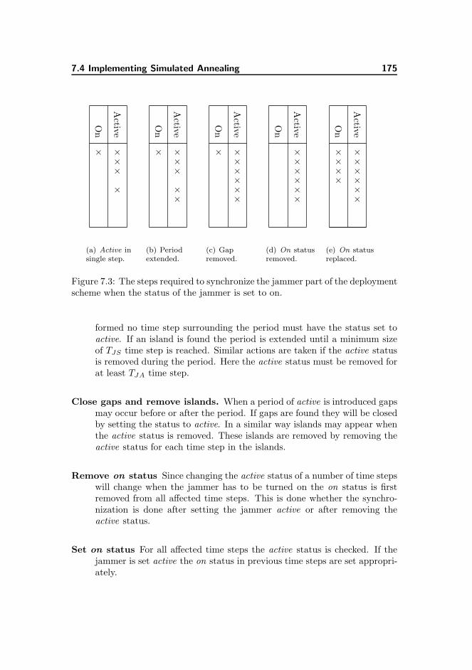
7.4 Implementing Simulated Annealing 175
On
Activ
e
× ×××
×
(a) Active insingle step.
On
Activ
e
× ×××
××
(b) Periodextended.
On
Activ
e
× ××××××
(c) Gapremoved.
On
Activ
e
××××××
(d) On statusremoved.
On
Activ
e
××××
××××××
(e) On statusreplaced.
Figure 7.3: The steps required to synchronize the jammer part of the deploymentscheme when the status of the jammer is set to on.
formed no time step surrounding the period must have the status set toactive. If an island is found the period is extended until a minimum sizeof TJS time step is reached. Similar actions are taken if the active statusis removed during the period. Here the active status must be removed forat least TJA time step.
Close gaps and remove islands. When a period of active is introduced gapsmay occur before or after the period. If gaps are found they will be closedby setting the status to active. In a similar way islands may appear whenthe active status is removed. These islands are removed by removing theactive status for each time step in the islands.
Remove on status Since changing the active status of a number of time stepswill change when the jammer has to be turned on the on status is firstremoved from all affected time steps. This is done whether the synchro-nization is done after setting the jammer active or after removing theactive status.
Set on status For all affected time steps the active status is checked. If thejammer is set active the on status in previous time steps are set appropri-ately.

176 The Metaheuristics Approach
7.4.4 Parameter Settings
The implementation of the Simulated Annealing algorithm offers a number ofparameters to be set. The parameter settings will influence the performance ofthe algorithm and the solutions found. The parameters include the start tem-perature, the temperature reduction factor, generation of a non-empty initialsolution (see Section 7.4.2), and the description of four different stopping crite-ria. The algorithm will stop when a maximum number of iterations is reached,if the current temperature gets lower than a preset end temperature, if the in-cumbent has remained unchanged for a number of iterations (referred to as idleiterations), or if a maximum running time has elapsed.
In determining the parameter settings two of the six scenarios used for testingthe mathematical model (see Section 6.7) are used. The sc1 scenario containsa single threat only, and it is chosen for determining the parameter settingsas it is likely that finding solutions to flights in this scenario is relatively fast.This is explained by the fact that the time it takes for the implementation ofthe algorithm to calculate the objective value in each iteration depends on thenumber of threats given in the scenario, and the sc1 scenario contains a singlethreat only. The second scenario for determining the parameters is the sc5
scenario. This is chosen since it contains three threats, and it is thus likelythat finding solutions to flights in this scenario will take an increased amountof time compared to finding solutions to flights in sc1. Since a valid optimalsolution to the flight in scenario sc6 is not found solving the mathematicalmodel using GAMS/CPLEX, this scenario is not used in tuning the parametersfor the algorithm. Short descriptions of the six scenarios are repeated in Table7.2.
It is essential that the algorithm provides good results within a very short periodof time. Therefore the algorithm is first run with varying values for the max-imum running time. The time limit is set to vary from 10 milliseconds to 120milliseconds. To ensure that most of the runs are terminated by the maximumrunning time stopping criterion, parameters describing the other three stoppingcriteria are set to refrain these from stopping the run. To perform the tests thestart temperature is set to 1,000,000, the maximum number of idle iterations is100,000, the end temperature is fixed at 10−20, and the reduction factor is setto 0.995. The survivabilities found for varying time limits are shown in Figure7.4.
For flights in scenario sc1 runs with maximum running times above 65 mil-liseconds are stopped as the end temperature is reached before the maximumrunning time has elapsed. None of the flights show an increase in survivabilitywhen the maximum running time is set higher than 85 milliseconds. To leave a
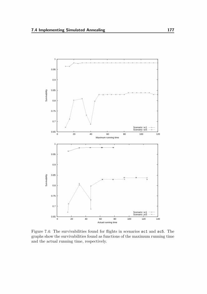
7.4 Implementing Simulated Annealing 177
0.65
0.7
0.75
0.8
0.85
0.9
0.95
1
0 20 40 60 80 100 120
Sur
viva
bilit
y
Maximum running time
Scenario: sc1Scenario: sc5
0.65
0.7
0.75
0.8
0.85
0.9
0.95
1
0 20 40 60 80 100 120 140
Sur
viva
bilit
y
Actual running time
Scenario: sc1Scenario: sc5
Figure 7.4: The survivabilities found for flights in scenarios sc1 and sc5. Thegraphs show the survivabilities found as functions of the maximum running timeand the actual running time, respectively.
178 The Metaheuristics Approach
margin for finding solutions to more complex scenarios the maximum runningtime is set to 100 milliseconds. This value is well within the 200 millisecondlimit given in Section 3.3.
For a given start temperature the reduction factor must be set so that a goodsolution is found before the maximum running time has been reached. If thereduction factor is set too low, i.e. the temperature decreases too fast, thealgorithm will not get to search larger parts of the search space before convergingtowards a local maximum. For the sc1 and sc5 flights the search spaces arerelatively small, and large parts of them can be evaluated within relatively fewiterations. Here the problem of having a small reduction factor is that it willmake the algorithm reach the end temperature before the maximum runningtime is reached. This limits the number of iterations in which the solutioncan be found. Since it is assumed that having the algorithm run for as manyiterations as possible will in general increase the objective value it is preferredthat the algorithm is not stopped by other stopping criteria than the maximumrunning time. Setting the reduction factor too high will keep the temperaturehigh throughout the execution of the algorithm. At high temperatures almostany candidate solutions will be accepted to replace the incumbent, and no goodfinal solution can be guaranteed.
Combinations of start temperatures and reduction factors are tested on the sc1
and sc5 flights. These tests show that varying the parameter values have verylittle effect on the survivabilities found. For the sc5 flight a reduction factorof more than 0.997 gives a decrease in survivability, while reduction factorsbelow 0.993 will make the algorithm stop as it reaches end temperature. Thereare no apparent differences in neither the survivabilities found nor the stoppingcriterion evoked when the temperature is varied between 100 and 5,000,000. Forthe sc1 flights having start temperatures below 500,000 result in the maximumtime being reached only when the reduction factor is above 0.997. Increasingthe start temperature to 5,000,000 does not change this. From these results thestart temperature is chosen at 500,000. The reduction factor must be set to avalue between 0.993, where the solving of the most time consuming problem isstopped at the end temperature, and 0.997, where the quality of the solutions isdecreasing. The reduction factor is set at 0.995, even though finding a solutionto the sc1 flight is not stopped by the maximum running time criterion at thisvalue. It is assumed that values above 0.995 is likely to decrease the quality ofthe solutions found, and it is assessed that better solutions are preferred eventhough they are found without invoking the maximum running time stoppingcriteria.
In determining the parameter settings an empty initial solution is being used.Section 7.4.2 describes another initial solution where the countermeasures offer-ing the best reduction of lethality are set active at each time step. Solutions
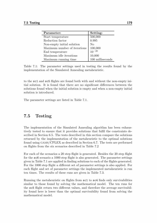
7.5 Testing 179
Parameter: Setting:Start temperature 500,000Reduction factor 0.995Non-empty initial solution NoMaximum number of iterations 100,000End temperature 10−20
Maximum idle iterations 10,000Maximum running time 100 milliseconds
Table 7.1: The parameter settings used in testing the results found by theimplementation of the Simulated Annealing metaheuristic.
to the sc1 and sc5 flights are found both with and without the non-empty ini-tial solution. It is found that there are no significant differences between thesolutions found when the initial solution is empty and when a non-empty initialsolution is introduced.
The parameter settings are listed in Table 7.1.
7.5 Testing
The implementation of the Simulated Annealing algorithm has been exhaus-tively tested to ensure that it provides solutions that fulfil the constraints de-scribed in Section 6.5. The tests described in this section compare the solutionsreturned by the implementation of the metaheuristic to the optimal solutionsfound using GAMS/CPLEX as described in Section 6.7. The tests are performedon flights from the six scenarios described in Table 7.2
For each of the scenarios a 20 step flight is generated. Besides the 20 step flightfor the sc6 scenario a 1000 step flight is also generated. The parameter settingsgiven in Table 7.1 are applied in finding solutions to each of the flights generated.For the 1000 step flight a different set of parameter settings is also applied. Foreach flight and set of parameter settings the implemented metaheuristic is runten times. The results of these runs are given in Table 7.3.
Running the metaheuristic on flights from sc1 to sc4 finds only survivabilitiessimilar to those found by solving the mathematical model. The ten runs forthe sc5 flight return two different values, and therefore the average survivabil-ity found here is lower than the optimal survivability found from solving themathematical model.
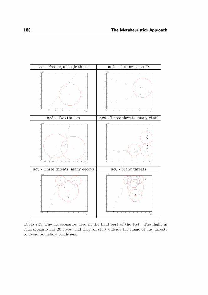
180 The Metaheuristics Approach
sc1 - Passing a single threat sc2 - Turning at an IP
0 1 2 3 4 5
x 104
0
0.5
1
1.5
2
2.5
3
3.5
4
4.5
5x 10
4
0 1 2 3 4 5 6 7
x 104
−0.5
0
0.5
1
1.5
2
2.5
3
3.5
4
4.5
x 104
sc3 - Two threats sc4 - Three threats, many chaff
−0.5 0 0.5 1 1.5 2 2.5 3 3.5 4 4.5
x 104
0
0.5
1
1.5
2
2.5
3
3.5
4
4.5x 10
4
0 1 2 3 4 5 6 7
x 104
1
2
3
4
5
6
x 104
sc5 - Three threats, many decoys sc6 - Many threats
−1 0 1 2 3 4 5 6 7
x 104
0
1
2
3
4
5
6
x 104
−1 0 1 2 3 4 5 6 7 8 9
x 104
0
1
2
3
4
5
6
7
8
x 104
Table 7.2: The six scenarios used in the final part of the test. The flight ineach scenario has 20 steps, and they all start outside the range of any threatsto avoid boundary conditions.
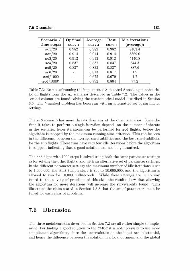
7.6 Discussion 181
Scenario / Optimal Average Best Idle iterationstime steps: surv.: surv.: surv.: (average):
sc1/20 0.982 0.982 0.982 8403.4sc2/20 0.914 0.914 0.914 8369.0sc3/20 0.912 0.912 0.912 5140.8sc4/20 0.837 0.837 0.837 644.3sc5/20 0.837 0.833 0.837 887.6sc6/20 - 0.813 0.817 1.9sc6/1000 - 0.675 0.679 1.7sc6/1000∗ - 0.792 0.804 77.2
Table 7.3: Results of running the implemented Simulated Annealing metaheuris-tic on flights from the six scenarios described in Table 7.2. The values in thesecond column are found solving the mathematical model described in Section6.5. The ∗-marked problem has been run with an alternative set of parametersettings.
The sc6 scenario has more threats than any of the other scenarios. Since thetime it takes to perform a single iteration depends on the number of threatsin the scenario, fewer iterations can be performed for sc6 flights, before thealgorithm is stopped by the maximum running time criterion. This can be seenin the difference between the average survivabilities and the best survivabilitiesfor the sc6 flights. These runs have very few idle iterations before the algorithmis stopped, indicating that a good solution can not be guaranteed.
The sc6 flight with 1000 steps is solved using both the same parameter settingsas for solving the other flights, and with an alternative set of parameter settings.In the different parameter settings the maximum number of idle iterations is setto 1,000,000, the start temperature is set to 50,000,000, and the algorithm isallowed to run for 10,000 milliseconds. While these settings are in no waytuned to the solving of problems of this size, the results show that allowingthe algorithm for more iterations will increase the survivability found. Thisillustrates the claim stated in Section 7.3.3 that the set of parameters must betuned for each class of problems.
7.6 Discussion
The three metaheuristics described in Section 7.2 are all rather simple to imple-ment. For finding a good solution to the CMOP it is not necessary to use morecomplicated algorithms, since the uncertainties on the input are substantial,and hence the difference between the solution in a local optimum and the global
182 The Metaheuristics Approach
optimum may be ”lost” in uncertainties. Using simulated annealing offers anacceptable trade-off between solution quality and computing time.
Each iteration will include an evaluation of a new candidate. When reaching lowtemperatures very few of these candidates will be accepted. To save computationtime in this part of the algorithm, the probability of accepting a new candidatecan be estimated, and then be used in accepting or rejecting candidate solutions,without performing the time consuming evaluation of each of these. Estimatingthe probability depends on both the function for calculating the probability andon the current candidate. This is not a trivial task to do.
It has been proven that the Simulated Annealing algorithm will converge towardsa global optimum given the right circumstances [40]. First, the Metropolis vari-ant of the algorithm is to be used, i.e. a number of iterations are performedat each temperature. If the temperature is decreased cautiously, and the num-ber of iterations at each temperature is large enough, the solutions found ateach temperature will reach a thermal equilibrium. This means that while theoptimal solution may not have been reached, the sum of signed fluctuations inthe objective values will be close to zero. If thermal equilibrium is obtainedat each temperature, and the Simulated Annealing is given unlimited time, theprobability of achieving one of the optimal solutions is one. For this to be truethe neighbourhood must be chosen in such a way that any feasible solution isreachable from any other feasible solution.
Although it is theoretically possible for the Simulated Annealing algorithm toconverge towards a global optimum, it can not be assumed to do so solvingthe CMOP. One of the reasons for this is the real-time requirement that anysystem solving the CMOP must fulfil. The 200 milliseconds time limit for findinga threat response (see Section 3.3) does not match the unlimited time requiredfor the Simulated Annealing to converge towards a global optimum.
While it is possible to reach all feasible solutions from all other feasible solutionsit may not always be easy to do so. If for instance the incumbent contains anumber of deployment intervals for the towed decoy equal to the number ofdecoys available, another deployment interval can only be introduced if one ofthe existing intervals gets eliminated. Removing a decoy deployment intervalrequires it to be removed step by step from either end. Toggling the state of thedecoy at a time step within the interval will split the interval into two intervals.If the number of intervals is already at the maximum number allowed, thissolution is not feasible. Having a neighbourhood where candidate solutions caneliminate an entire deployment interval completely will make it easier for themetaheuristic to escape local optima.
In the mathematical model, described in Chapter 6, the penalty for having a
7.6 Discussion 183
countermeasure turned on or active in a given time step is ε = 0.0001. Thesmall value is used because the optimal value, disregarding the penalty, wouldbe relatively close to the value returned by GAMS/CPLEX. For the metaheuristicthis small value may not be an advantage. In the first part of the run a solutionwith countermeasures turned on without being necessary, e.g. when the aircraftis outside the range of any threat, will only present a slightly worse solutionthan the incumbent, and the probability of it being accepted is relatively large.This may result in the introduction of unnecessary deployment intervals, and asexplained above these may not easily be removed.
As with the mathematical model a large part of the effort in implementingthe metaheuristics has been focussed on synchronizing the time steps where acountermeasure is active with the time steps where it is on. While this syn-chronization seems to work, it has not been tested for all possible combinations,and situations may exist in which the synchronization will return a non-feasiblesolution. Leaving out the variables describing when the jammer is turned onand when the towed decoy is deployed, as suggested in Section 6.8, will makethe synchronization both easier to implement and faster to run.
The Simulated Annealing algorithm can be used in combination with otheralgorithms and metaheuristics. An example of this is the algorithm describedin Section 7.4.2 for finding an initial solution. The Steepest Ascent algorithmcan be used in a post-processing stage of the results given by the SimulatedAnnealing. If the Steepest Ascent algorithm is run long enough it is ensuredthat at least a local optimum is found.
Since no countermeasures should be deployed outside the range of threats inthe scenario, omitting most of the time steps where the aircraft is outside allranges from the problem description would reduce the size of the problem, thusimproving the efficiency of the algorithm. Removing all these time steps caneffect the solution found since a countermeasure may need to be turned on/de-ployed/dispensed ahead of the period in which it is within the range of a threat.Due to the limited amount of towed decoys aboard the aircraft it may also benecessary to keep a decoy deployed when the aircraft flies between the rangesof two threats. Care should therefore be taken if it is decided to reduce theproblem size by omitting part of these steps.
During flight the solutions found at a given time step can be shifted one timestep and be used as initial solution for a run in the following time steps. Doingthis may lessen the time it takes to find good solutions for the following timesteps and hence the allowed running time can be decreased. When shifting thesolution one time step at each run, already found deployment intervals can beshifted out of the deployment scheme. When this happens to a decoy deploymentor a chaff dispensing the total number of allowed deployments/dispensings must
184 The Metaheuristics Approach
be increased accordingly.
The tests described in Section 7.5 show how the number of threats influencesthe number of iterations that can be performed within a limited amount of time.This influence is caused by the calculation of the objective function, since thisis the only part of the algorithm where the number of threats has an impact. Iffinding the objective value was done more efficiently, e.g. by following the stepsdescribed in 7.4.1, the effect of multiple threats will decrease.
7.7 Conclusion
With the implementation of the Simulated Annealing it is shown that it ispossible to find good solutions to the CMOP within short time. To flights withno more than 20 time steps the solutions found will often be either optimal,or close to an optimum. For problems involving more time steps or threatsthan the ones tested in Section 7.5 the current implementation of the SimulatedAnnealing algorithm may still be too slow. No actions have been taken toimprove the solutions for these problems within the time limit.
For the flights constructed good solutions are found within 100 milliseconds. Itis believed that good solutions may also be obtained for larger problems if theparameter settings were optimised according to the size of these problems.
It is concluded that Simulated Annealing is an appropriate choice of metaheuris-tic for solving the CMOP. It is, however, not evident that it is the metaheuristicbest suited to perform the task. To find the metaheuristic that will find thebest solutions within a limited time will require more metaheuristics to be im-plemented, and more tests to be performed.
Chapter 8
Comparing Approaches
The four approaches described in this work represent four different technologiesthat can be used in designing a DSS for fighter pilots. In this chapter the fourapproaches are compared, and pros and cons of each technology are described.The approaches are compared with regards to five of the six design requirementsdescribed in Section 3.3: real-time, hardware, updateable, trustworthy, and us-able. For each of these requirements the approaches are marked from one to fivewhere five is the best. These marks are the result of a subjective assessment bythe author, and from the marks the approach best suited for further develop-ment is found. The sixth design requirement, a usable user interface, has beenomitted in this comparison, since no effort has been done to develop a suitableinterface to either of the systems developed.
8.1 The Approaches
In Section 3.3 it is estimated that a DSS must be able to suggest evasive actionsto the pilot within 200 milliseconds from the time a change in the scenariooccurs. It is assumed that this response time is obtained running the DSS on anaircraft computer. Since neither of the systems developed in this work has beenrun on such a computer all the response times reported are estimates based on
186 Comparing Approaches
the computation times found using the computer systems described in AppendixE.
For all approaches it is assumed that uploading mission data and updates tothe systems can be easily done during the pre-flight preparation of the aircraft.How this is done is beyond the scope of the work.
8.1.1 Prolog
The Prolog program described in Chapter 4 uses a set of rules for a pilot tofollow to perform evasive actions in a hostile environment. These rules arecombined with a knowledge base containing descriptions of threats and howthey are mitigated. Descriptions of the current scenario are also used by theprogram for suggesting actions.
Real-time. Traditionally the execution of Prolog programs is considered slow.This is due to the way a Prolog interpreter will compare every state ob-tained to a number of rules to see whether a rule can be matched. Theprogram described in Chapter 4 has been run using B-Prolog on the laptopPC described in Appendix E. With this configuration neither of the runswas registered to take more than 150 ms. To this period of time the timeit takes to register data about the current scenario must be added, as mustthe time it takes to present the output of the program to the pilot. In thischain of actions running the Prolog program is considered to be the mosttime consuming. It should be noted that adding to the complexity of thescenario or to the size of the knowledge base will increase the time usedby the Prolog interpreter. This may influence the ability for the Prologprogram to give real-time performance and hence it is rated the mark 4.
Hardware. Although it is unlikely that a Prolog interpreter is currently in-stalled on an aircraft computer it is assumed that writing such an inter-preter is relatively easy (see Section 4.1). Input to the Prolog system willcome from either onboard systems, such as the MWS and the RWR, or itwill be given pre-mission. The developed system requires data to be writ-ten to Prolog files which may be consulted at a fixed interval. Convertingdata from devices attached to the aircraft data bus to either a Prolog fileor directly input to the Prolog interpreter is assumed a minor task. All inall the Prolog approach receives the mark 4 for fulfilling the requirementsset by the aircraft computer and hardware.
Updateable. The Prolog program was developed in a relatively short time.This suggests that both minor updates and major rewrites can also be
8.1 The Approaches 187
done in a short time. If it can be assumed that the logic behind theProlog program does not change, the updates necessary will be limitedto the knowledge base and the programs for dispensing expendables. Inthe Prolog program these data are kept in separate files and the updatesconcern these files only. The Prolog approach is rated the mark 5 forfulfilling the updating requirement.
Trustworthy. The Prolog based DSS will suggest every feasible solution to allproblems presented to it. Whether these problems are the results of real-world threats, or merely stems from false alarms from e.g. the MWS, is ofno concern to the program. Input can come from different sources, eachof which has a probability of supplying erroneous information and falsealarms. If input from one source is erroneous the output from the programis likely to be erroneous too. The probability of the program suggestionactions that does not match the real-world scenario is thus bigger than itis for each of its input sources to deliver erroneous input. This problemhas been described in [52].
The experienced pilot will have a perception of how reliable each of theon-board sensor system is, and he will respond to the warnings given bysuch a system according to this reliability. With the introduction of theProlog program the sources of warnings will be hidden from the pilot, andthe perception of reliability will be gone. For fulfilling the requirement ofa DSS to be trustworthy the Prolog program is rated the mark 3.
Useful. The program will find all feasible actions to scenarios given. There isno ordering of the solutions, and the task of finding the best applicablesolution is left to the pilot. The more threats the system needs to findactions for the more actions it will probably find. Since more threats in thescenario will increase the pilot’s workload, an increase in the informationpresented to him by the system is not beneficial.
The Prolog system will register if a previously deployed countermeasuremay currently have an effect on threats in the scenario. Also the amountof expendables is registered for the system to see if a given countermeasureprogram can be executed. Knowledge about threats that the aircraft willencounter in the near future is not used by the program. Thus neither thebest sequence of deploying countermeasures, nor the probability of havingenough expendables for the rest of the mission is found.
The Prolog program is basically categorical, and although any relationscan be described with some uncertainty, it does not take the uncertaintyon the observations into account. Unlike the other three approaches theProlog program may improve the probability of the survival of the aircraftwithout giving an estimate of the improvement. If the notion of surviv-ability was introduced in the program it may help in ordering the solutions
188 Comparing Approaches
found at each time step. The overall usefulness of the Prolog program israted the mark 3.
8.1.2 Bayesian Network
For the EW domain the variables in a BN refer to e.g. the presence of radarradiation, approaching missiles, or warnings issued by sensor systems on-boardthe aircraft. For each relation between a variable and the variables it dependsdirectly upon the dependencies are described using a dependency table. Whenchances to the probability of a variable being in a given state is changed theBN is updated, and all related dependencies are re-calculated. For the BN thesurvivability is the probability of the variable Survive being in the Survive state.The best action yields the highest survivability.
Real-time. The time it takes to update a BN depends on the number of vari-ables and dependencies in the BN. Therefore expanding the BN to be ableto accommodate more scenarios and a broader range of actions is likelyto slow down the execution. Speeding up the execution may be done bywriting a program that is dedicated to finding the best combination ofactions with the model developed, and not be dependent on the HUGINtool.
For finding the best combination of actions to a given scenario each com-bination is set using the HUGIN user interface and the survivability fromthis combination is then calculated. Each of these calculations is done inwhat appears to be real-time. The number of combinations to evaluate isfairly small and it is assumed that the total time it will take to calculatethe survivabilities for all combinations is well below one second, and prob-ably within the 200 ms limit. This can be verified by writing a programthat interacts with HUGIN and performs all the survivability calculations;this has not been done. Overall the BN approach is rated the mark 3 forthe ability to fulfil the real-time requirement.
Hardware. The HUGIN software may not easily be ported to an aircraft com-puter. If HUGIN, or another PC-based BN tool, is used for the develop-ment of a BN, the model itself may be ported to an aircraft computer.Writing a program for this computer than can read the ported model andmaintain and update a BN may be just as easy as the implementation ofa Prolog interpreter as previously mentioned. The mark 4 is given to theBN approach for fulfilling the hardware requirement.
Updateable. Developing and maintaining a BN has proven to be very cum-bersome. The dependency tables involved may become very large, and
8.1 The Approaches 189
updating these by hand is difficult. If statistical data about the relationsbetween variables in the BN are available it may be possible to update theBN, or parts hereof, using Structural Learning.
Introducing new threats or countermeasures to the BN is done by intro-ducing new variables or new states in existing variables. This can notbe done without updating large parts of the BN since all variables beingdirectly influenced by the changes must also be changed. All in all the BN
approach gets the mark 2 for the ability to be updated.
Trustworthy. One of the advantages with the BN developed is that it is de-signed to manage the probabilities of sensors reporting false alarms. Evenif the probability of a sensor issuing a warning is 100%, the probabilityof this being wrong is incorporated in the model. As long as the modelused for the BN can be considered trustworthy so can the results found.For this the BN approach is given the mark 5. One may argue that theBN developed is not entirely trustworthy, and that the mark should beno more than 3 or 4. It is deemed that the model is as trustworthy asthe domain knowledge upon which it is build, and therefore the mark 5 isobtainable if sufficient data are given.
Useful. For every scenario presented to the BN examining combinations of pos-sible actions will result in the combination of actions yielding the highestsurvivability. This offers an improved usability compared to the Prologprogram since the workload of the pilot is not increased by the DSS if thenumber of threats in the scenario increases.
Since expanding the BN is cumbersome, the number of e.g. missiles thatis known by the BN is very limited. This means that the probability ofthe pilot encountering threats not known by the BN is relatively high.While this will not prevent the system from finding a good combinationof actions, the pilot may not be convinced that this combination is in factthe best. The number of actions in the BN is also very limited, and thistoo will influence the usefulness of the BN.
When a manoeuvre is necessary for the aircraft to obtain a break lock thesystem will not describe this manoeuvre. Adding this functionality to thesystem would clearly improve its usefulness. Without it the usefulness ofthe BN-based DSS receives the mark 3.
8.1.3 Mathematical Model
The mathematical model is implemented to solve a problem different from theproblem solved using the Prolog program or the BN model. Where the focus inthe first two approaches is on providing solutions to the current threat scenario
190 Comparing Approaches
the focus with the implementation of the mathematical model is on finding thebest sequence of countermeasure deployments during an entire mission. Findingthe best solution to any given time is considered trivial and is basically done bysimple table look-ups. It is assumed that some knowledge about threats that willbe encountered by the aircraft in the near future is known. The mathematicalmodel is written in the GAMS language and it is solved using the CPLEX solver.
Real-time. Using GAMS/CPLEX solving problems with approximately 20 timesteps will take from a few seconds to several hours, depending on thecomplexity of the scenario. This suggests that solving the mathematicalmodel to optimality with currently available hardware and software cannot be guaranteed in real-time. For this the approach gets the mark 1.
Hardware. Using the newest computer technology for running the GAMS/CPLEX software the computation times experienced in this work maybe reduced substantially. It is unlikely that this technology will reducethe computation time enough for the system to become real-time, and itis equally unlikely that the technology will soon be implemented in exist-ing fighter aircraft. For meeting the requirement that a DSS must be ableto run on an aircraft computer this approach gets the mark 1.
Updateable. Changing the lethality of the involved threats, or adding newtypes of threats to the scenario, is relatively easy, as long as the newthreats behave similar to the existing threats. Also changing the reductionfunctions for each countermeasure can be done with a minimum of effortsince these functions are described using simple look-up tables.
Adding more countermeasures to the mathematical model will result inthe addition of constraints to the model. As long as the added counter-measures have time relations comparable to those of the already includedcountermeasures this is a trivial task. This kind of countermeasures caneither be described using the five-phase description from Section 6.5.1, orif they are expendables the constraints can be compared to those relatedto chaff dispensing. Another very important requirement to new counter-measures is that they work on RF based threats. If that is not the casethe lethality will need to be redefined. The related reductions of lethalitywill also need to be computed as functions of the electromagnetic band inwhich they work.
Since updating the mathematical model with new threats and threat sce-narios is likely to be the most frequent updates to the system the approachusing the mathematical model gets the mark 4 for the ability to be up-dated.
Trustworthy. If it is assumed that knowledge about the type and positions ofenemy threats are the results from intelligence reports, the solutions found
8.1 The Approaches 191
using the mathematical model will not suffer from the dependency of on-board sensors as e.g. the Prolog program does. As long as the descriptionof threats used to find the optimal sequence of actions matches the realworld the results can be trusted. As this can not always be guaranteedand information from e.g. the RWR is needed to update the threat scenariothe system becomes less trustworthy and the mark is set to 3.
Useful. Since the performance of a system based on finding the optimal solutionto the mathematical model is far from real-time the usefulness of such asystem appears as quite small. It is assumed that positions of threatsare known before the aircraft embarks on the mission. If this informationis available long enough for GAMS/CPLEX to provide a solution beforethe mission is initiated this solution may still be useful to the pilot. Theoptimal solutions found solving the mathematical model can also be usedin tuning the parameters for use in the metaheuristic. The mathematicalmodel thus proves its usefulness in other areas as well.
In Section 2.3 it is mentioned that IR guided missiles may be consideredthe greatest threat towards aircraft. Since the mathematical model doesnot find solutions to scenarios including IR guided missiles the usefulnessof the mathematical model diminishes.
The results from the system will describe when a countermeasure needs toget deployed, and which threat it is mitigating. How this deployment isto be done, and which manoeuvres that must accompany it is not given.This brings the usability of the mathematical model down to the mark 2.
8.1.4 Metaheuristics
The implemented Simulated Anneling metaheuristic will solve the same prob-lems as solved by the mathematical model. The differences between these meth-ods are mainly found in the value of the solutions, and the time it takes to findthem. Where GAMS/CPLEX will use a long time to find the optimal value toa problem, the metaheuristic will often find a suboptimal solution to the sameproblem in much less time. As mentioned in Section 7.1 the description of abattlefield scenario will often be so deficient that the optimal solution foundby the GAMS/CPLEX method may not be any better than any solution foundusing the Simulated Annealing metaheuristic.
Real-time. One of the advantages of a metaheuristic such as Simulated An-nealing is that the time it is allowed to find a good solution can be usedas a stopping criterion, and when stopped the currently best found solu-tion is returned. This means that Simulated Annealing can probably be
192 Comparing Approaches
used to find good feasible solutions within the 200 ms limit set in Section3.3. Since the solution to the problem at a given time can build upon thesolution found at the previous time step, the time it takes to find a goodfeasible solution will be even less than the times found in Chapter 7. Forthis the mark for the real-time requirement is set to 4.
Hardware. The success of the Simulated Annealing depends on the numberof iterations it is allowed to perform before being stopped. For a fixedrunning-time this number of iterations depends on both the program im-plementing the metaheuristic and the hardware on which it is run. Evenif an aircraft computer does not perform as fast as the laptop PC used forrunning the implementation described in Chapter 7 it will not render theuse of the metaheuristic impossible; only the quality of the solutions foundmay be deteriorated. The mark for matching the hardware on-board theaircraft is set to 3.
Updateable. Updating the scenario for the metaheuristic can be done by up-dating the files that describes the scenario and the reduction of lethalityby the countermeasures. The format of these files is the same for the im-plementation of the metaheuristic as for the files that are included in theGAMS program. Updating the program itself to include other countermea-sure or to be able to counter IR guided missiles will require parts of theprogram running the metaheuristic to be rewritten. Since the updating ofthe implementation of the metaheuristic is similar to updating the systemusing the mathematical model it too gets the mark 4 for the ability to beupdated.
Trustworthy. Compared to the system using the mathematical model themetaheuristic system can, due to its ability to deliver real-time solutions,respond to changes in the scenario as they occur. This will bring the markfor trustworthiness up to 4.
Useful. This system suffers from the same drawbacks as the system solvingthe mathematical model. That it may operate in real-time increases theusability of the system and it receives the mark 3 for this.
8.2 Comparison
The marks given for each of the five design requirements to the four approachesare collected in Table 8.1. Comparing the approaches can also be done bystudying the web plots in Figure 8.1. Generally the best approach will be theone with the largest area in the web plot.
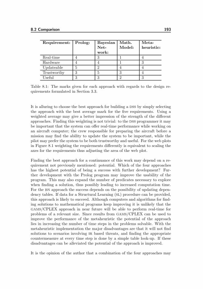
8.2 Comparison 193
Requirement: Prolog: BayesianNet-work:
Math.Model:
Meta-heuristic:
Real-time 4 3 1 4Hardware 4 4 1 3Updateable 5 2 4 4Trustworthy 3 5 3 4Useful 3 3 2 3
Table 8.1: The marks given for each approach with regards to the design re-quirements formulated in Section 3.3.
It is alluring to choose the best approach for building a DSS by simply selectingthe approach with the best average mark for the five requirements. Using aweighted average may give a better impression of the strength of the differentapproaches. Finding this weighting is not trivial: to the DSS programmer it maybe important that the system can offer real-time performance while working onan aircraft computer; the crew responsible for preparing the aircraft before amission may find the ability to update the system to be important, while thepilot may prefer the system to be both trustworthy and useful. For the web plotsin Figure 8.1 weighting the requirements differently is equivalent to scaling theaxes for the requirements thus adjusting the area of the web plot.
Finding the best approach for a continuance of this work may depend on a re-quirement not previously mentioned: potential. Which of the four approacheshas the highest potential of being a success with further development? Fur-ther development with the Prolog program may improve the usability of theprogram. This may also expand the number of predicates necessary to explorewhen finding a solution, thus possibly leading to increased computation time.For the BN approach the success depends on the possibility of updating depen-dency tables. If data for a Structural Learning (SL) procedure can be provided,this approach is likely to succeed. Although computers and algorithms for find-ing solutions to mathematical programs keep improving it is unlikely that theGAMS/CPLEX approach in near future will be able to perform real-time forproblems of a relevant size. Since results from GAMS/CPLEX can be used toimprove the performance of the metaheuristic the potential of the approachlies in increasing the number of time steps in the problems solvable. With themetaheuristic implementation the major disadvantages are that it will not findsolutions to scenarios involving IR based threats, and finding the appropriatecountermeasure at every time step is done by a simple table look-up. If thesedisadvantages can be alleviated the potential of the approach is improved.
It is the opinion of the author that a combination of the four approaches may
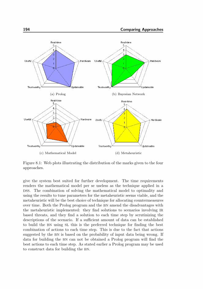
194 Comparing Approaches
(a) Prolog (b) Bayesian Network
(c) Mathematical Model (d) Metaheuristic
Figure 8.1: Web plots illustrating the distribution of the marks given to the fourapproaches.
give the system best suited for further development. The time requirementsrenders the mathematical model per se useless as the technique applied in aDSS. The combination of solving the mathematical model to optimality andusing the results to tune parameters for the metaheuristic seems viable, and themetaheuristic will be the best choice of technique for allocating countermeasuresover time. Both the Prolog program and the BN amend the disadvantages withthe metaheuristic implemented: they find solutions to scenarios involving IR
based threats, and they find a solution to each time step by scrutinizing thedescriptions of the scenario. If a sufficient amount of data can be establishedto build the BN using SL this is the preferred technique for finding the bestcombination of actions to each time step. This is due to the fact that actionssuggested by the BN is based on the probability of input data being wrong. Ifdata for building the BN can not be obtained a Prolog program will find thebest actions to each time step. As stated earlier a Prolog program may be usedto construct data for building the BN.
Chapter 9
Further Work
This chapter suggests further work for improving the results from the four ap-proaches previously described. Also methods for testing the results from theapproaches are described, and finally a few approaches which may be good can-didates for further investigation are suggested.
9.1 Current Approaches
The work with the four approaches has been focussed on providing enough ma-terial to evaluate the concept of each approach as the technology to use in a DSS
for fighter pilots. To fully understand the potential of these approaches furtherwork needs to be done for each of them. Besides improving the understand-ing the tasks described will either improve the usefulness of each approach orlessen the time it takes to suggest actions to the pilot. Some of these tasks aredescribed here.
196 Further Work
9.1.1 Prolog
In Chapter 4 it is mentioned that defining the set of rules to build the Prologprogram upon is best done in iterations, where an implementation of the currentset of rules is evaluated, new rules can be added, and old rules may be removed orchanged. Conducting these iterations will require the co-operation of a numberof experts within the EW domain.
The Prolog program returns every feasible solution to any scenario describedto it. The solutions are composed of combinations of manoeuvres and counter-measures. In performing the proper evasive actions the pilot will benefit fromthese combinations being prioritized. The prioritization can be done by eitherthe increase in survivability given by the combinations, or by how easy they areto perform given the current status of countermeasures and direction of flight.On a graphical display the solutions can be presented in such a way that theperson testing the system will see which threat each combination is mitigating.
The Prolog program does not take advantage of any knowledge about threatsthat will be encountered in the near future. Doing so will require a set of rulesdescribing this to be formulated. Even though this formulation is not a trivialtask, it can be introduced as part of the iterative improvement of the set ofrules.
9.1.2 Bayesian Network
The time it takes for HUGIN to propagate evidence throughout the networkdepends on the number of nodes in the network. Section 5.3.2 explains that 36combinations of states within four action nodes must be tested to find the onegiving the highest survivability for a threat scenario. Since these combinationsare mutually exclusive a single action node with 36 states can be constructedinstead. This reduces the number of evidence propagations for each change inthe BN from 36 to just one, which will result in a decrease of the total runningtime.
The BN model lacks the ability to determine the manoeuvre resulting in thebest survivability. As it is any manoeuvre is preferred since deploying a coun-termeasure will almost always require a manoeuvre. If angles are introduced intothe model the manoeuvre providing the best survivability can be found. Thedrawback of introducing angles is that the time it takes to propagate changesthroughout the network is likely to increase.
9.1 Current Approaches 197
The model includes only three types of countermeasures: flares, chaff, and jam-mer. If more countermeasures are included, and both new and existing coun-termeasures are described by a number of programs, the model will be closer todescribing the situation for a fighter pilot. This will make it easier for e.g. afighter pilot to perform an evaluation of the abilities of a BN approach.
Large parts of the BN model can be build using Structural Learning (SL). Thelearning feature offered by HUGIN seems to provide good results and it is thusa good candidate for performing the SL, although other tools for doing this maybe investigated. Doing SL requires statistical data to be available. Statisticaldata from trials and real-life experience may be sufficient for the task, butthe nature of these data makes them difficult to acquire. Synthetic data, e.g.provided by the Fly-In tool, may have the same characteristics as data fromreal aircraft. Gathering synthetic data can be a time-consuming task dependingon the number of parameters included in the simulations. It will require morein-depth analysis to determine the parameters and the values of these to basethe simulations on. Writing a Prolog program for delivering parts of these datamay prove to be a viable approach; for instance in deciding proper angles formanoeuvres in conjunction with countermeasure deployments.
9.1.3 Mathematical Model
In Chapter 8 it was ascertained that solving the mathematical model using theGAMS/CPLEX approach is unlikely to produce usable results in real-time. An-other use of the model is to find optimal solutions for problems that can be usedin tuning parameters for the metaheuristic approach. Since parameter tuningis best done on problems similar to those which must be solved using the meta-heuristic the implementation of the mathematical model must be able to solvethese problems. In Section 6.4.3 it is estimated that a time frame may includeup till 1500 time steps. Since finding the optimal solution to the CMOP with20 time steps may take several hours with the GAMS/CPLEX approach, findingan optimal solution to a problem with 1500 time steps can not be done withinreasonable time. Introducing more advanced OR techniques may be helpful infinding solutions to problems of this size faster, as relaxing the integer require-ments may also prove to be beneficial.
The mathematical model is used to optimise the survivability for the aircraftflying a route defined by a set of IPs. A similar model may be developed to findIPs describing the route providing the optimal survivability. As route planningis a task that is most often carried out before a mission is initiated, finding asolution in real-time is no requirement.
198 Further Work
9.1.4 Metaheuristic
As mentioned in Section 7.6 the initial solution to all but the first run of theSimulated Annealing may be a modification of the solution found at the previ-ous run. The implementation of the metaheuristic may take advantage of thispossibility. This initial solution might need to be modified if new threats haveoccurred, or if the battlefield scenario has otherwise changed.
In [40] the techniques for accelerating Simulated Annealing are classified intothree categories: designing a faster algorithm by improving the cooling sched-ule, the neighbourhood, or the objective function; using hardware accelerationwhere time consuming parts of the algorithm is implemented in hardware; andfinally parallelising the algorithm to take advantage of multiple processors. TheSimulated Annealing implementation in this work has been evaluated using onlya single neighbourhood definition and a single definition of the objective func-tion. Experimenting with more implementations of these, as well as a varietyof cooling schedules, may result in better performance within the fixed timeinterval given.
Since this work is of an exploratory nature implementing parts of the SimulatedAnnealing in hardware is considered beyond the scope. If a DSS is being im-plemented, and the choice of technique to use for this is a Simulated Annealingimplementation, experiments using hardware acceleration need to be carriedout. The aircraft computer running a DSS will probably be dedicated to thisand having hardware running parts of the Simulated Annealing algorithm inthis computer may thus be feasible. A disadvantage by having parts of the DSS
implemented in hardware is that updating the DSS is likely to be more difficult.
According to [15, 40] parallelising the Simulated Annealing has been the subjectof several studies. The parallelisation can be done in different ways, three ofwhich are described here. The simplest way is to run an instance of the algorithmon each available processor. The instances would be stopped at the same timedue to the fixed running time allowed, and the best solution is chosen. Theimmediate advantage of this approach is that it is relatively easy to implementsince a minimum of synchronization between the processors is involved. If theinstances are given the same initial solution and a very limited time to improveit, they may all explore the same part of the search space. It is not unlikely thatthe solutions found will be close, and there will little benefit from an increasein the number of available processors.
Introducing communication between the processors may result in better results.Each instance of the algorithm may search for solutions near the incumbentand report to the other instances when an accepted solution is found. This
9.2 Testing with Flight Data 199
solution will then be the incumbent for all instances in the continued search.This parallelisation will search larger parts of the search space during the fixedcomputation time allowed and the results is likely to be improved.
Having each processor working on a subproblem instead of the full problem mayimprove the solution found to each subproblem. For n processors the problemsolved by the first processor may then contain only the first 1/n time steps, thenext problem will describe the next 1/n time steps, and so on. The solutionsfound by each instance of the algorithm is reported in due time and everyprocessor will have the fixed computation time allowed for solving only 1/n’th ofthe problem. While the quality of the solutions to each of these subproblems willhopefully improve it can not be guaranteed that the combination of solutionsto the subproblems constitute a good solution to the entire problem. Whichparallelisations best suited for improving the results found using the SimulatedAnnealing may be the subject of further work.
With the implementation of the Simulated Annealing reported here the choicesof cooling schedule, neighbourhood, and objective function may be subject forre-evaluation. Also the choice of metaheuristic may be re-evaluated. In Section7.2.4 it is mentioned that the Simulated Annealing performs at its best if givenenough time and if data describing the problem are uniform. Since the natureof the CMOP and the environment in which it needs to be solved offers neitheroptimal time conditions nor uniform data the choice of Simulated Annealingas metaheuristic may not be the best and other metaheuristics needs to beconsidered as well.
9.2 Testing with Flight Data
The four approaches have all been tested using synthetic data from scenariosfabricated to this purpose only. The Prolog program has been tested usingwarnings issued from the RWR and the MWS in well defined scenarios. Thesewarnings are all caused by threats in the scenarios and the possibility of falsewarnings has not been exploited. Testing both the mathematical model andthe metaheuristic implementations are done using a high-level description ofscenarios where interaction with sensors on-board the aircraft is ignored. Testingwith flight data instead of data constructed for test only may reveal flaws in thedesign of each of the approaches. It is recommended that this type of testing iscarried out before further development is commenced.
200 Further Work
9.2.1 Flight Simulator
At DDRE there has been some experience using the PC-based Falcon 4.0 flightsimulator for supplying data to a tactical trainer [18]. These data can alsobe used for testing a PC-based DSS, where data may either be fed live to thesystem, or it may be recorded for later off-line data processing. With the livedata feed the flight simulator will deliver flight data at a given frequency. TheDSS then finds the combination of actions with the highest survivability giventhe flight data and these actions can be displayed on a monitor adjacent to theone showing the flight simulator.
If the DSS is run on the PC also running the flight simulator it might be difficultto meet the 200 milliseconds response time requirement. Therefore a two-PCsetup is suggested; one running the flight simulator and one running the DSS.The connection between the computers can be established using an ordinarycomputer network cable. The delay in the transmission of data between theflight simulator and the DSS can be ignored since finding solutions to the scenariowill still be the time consuming part of the process.
Falcon 4.0 will only supply the DSS with RWR data and the current amountof chaff and flares. While this is a drawback for testing the influence by MWS
warnings and jammer data the connection between the Falcon 4.0 flight simu-lator and a DSS is still considered a good approach for performing flight datatests.
9.2.2 Flight Recorder Data
For some aircraft an on-board flight data recorder may deliver input to the testof a DSS. These data may consist of frequently collected aircraft positions andorientations, airspeed, sensor warnings, etc. An advantage with these data isthat they carry the uncertainties experienced by the sensors aboard a real-lifeaircraft. A drawback is that the effect of actions suggested by the DSS will notbe part of the data. While it may be possible to infer actions taken by thepilot, mapping these to possible actions suggested by the DSS may prove to bedifficult.
9.3 Other Techniques 201
9.2.3 Live Data Feed
The best way to test the actions suggested by a DSS will be to present theresults to the fighter pilot during flight. Since the space in most fighter aircraftis limited it may be difficult to fit a DSS prototype into the cockpit. The testof a DSS does not require the aircraft to be a fighter aircraft, and it might aswell be installed in a larger aircraft, e.g. in a military transport aircraft. Heredata can be acquired from a MIL-STD-1553B (see Section 3.5.1) bus in muchthe same way as in a fighter aircraft1. A transport aircraft may be equippedwith largely the same countermeasures as a fighter aircraft and although thespeed and manoeuvrability of the transport aircraft is different from those ofthe fighter aircraft it is still possible to measure the effects of actions suggestedby the DSS.
To ensure input data from on-board warning system such as RWR and MWS thetesting of the system needs to be performed flying over threats. Flying a trans-port aircraft over enemy territory can not be regarded as optimal conditions fordoing countermeasure or DSS tests. For this the NATO Air Force ArmamentsGroup organise a series of tests with the participation of equipment and air-craft from different NATO countries. Here the aircraft overfly real or simulatedthreats to test the effect of aircraft countermeasures. Two series are organised:trial MACE covers RF based threats and trial EMBOW covers testing againstelectro-optical systems including IR threats [43].
9.3 Other Techniques
Other techniques than the four described in this work may be viable for the con-struction of a DSS for fighter pilots. Some of the candidates that were discussedduring the work are described in this section.
9.3.1 Constraint Logic Programming
Constraint Logic Programming (CLP) is a combination of two declarative pro-gramming paradigms: logic programming and constraint solving. With logicprogramming variables have the scope of the current predicate only. In CLP
constraints are introduced to represent relations between variables throughout
1Not all military transport or fighter aircraft are equipped with the MIL-STD-1553Bdatabus. Acquiring data from a non-standard databus may be inconvenient but still pos-sible.
202 Further Work
a given domain such as trees and sets. Handling these constraints is done usinga programming language that adds to the functionality of Prolog [56]. Generallythere is a strong connection between Prolog and CLP, and many Prolog inter-preters offers some degree of CLP, while compilers dedicated to CLP will oftenbe able to compile Prolog programs.
CLP can be used for adding functionality to the Prolog program described inChapter 4, and according to e.g. [56] it may enhance both the productivity ofsoftware development and software maintainability. Several CLP systems can beinvestigated for this, e.g. the B-Prolog system introduced in Chapter 4 and theECLiPSe system [2].
9.3.2 Artificial Neural Net
Using an Artificial Neural Net (ANN) a number of neurons can represent thesame set of variables as introduced in the BN approach. While the results witha BN is found by propagating probabilities throughout the entire network, theresults from a ANN is found using a number of functions integrated with therelevant sequences of neurons from the input to the output.
Updating the dependency tables in the BN has shown to be a disadvantage withthis approach. Learning the structure and dependency tables using SL requiresrepresentative data for all combinations of states within the variables of the BN.If only parts of this set of data is available SL will come short of providing ausable BN. If a learning ANN is used instead the setup of functions and weighswithin the network will be adjusted according to the data it can be trained with.If this training is done using e.g. data from a flight simulator it may show thatdata representing all combinations of states are not necessary to train the ANN
to provide good solutions.
In [38] an ANN is taught to play poker without knowing any expert strategies.The ANN here showed the ability to play and win a poker game where knowledgeof cards held by the opponents was unavailable. A similar teaching scheme canbe applied to an ANN for finding actions to be performed by a pilot when ground-based threats emerge. Here the opponent represent the enemy, the card held bythe opponent are hidden to the system in much the same way as the numberand positions of threats, and finally information about approaching missiles canbe compared to the revealed community cards in Texas Hold’em poker.
Exploring the ANN approach can be done by either developing relevant softwareor by using commercial software such as the Neural Net Toolbox in MATLAB.

9.3 Other Techniques 203
9.3.3 Stochastic Programming
Stochastic Programming is a framework for modelling uncertainty involved inoptimisation problems. The mathematical model described in Chapter 6 de-scribes a deterministic optimisation problem where the parameters describingboth the threats and the effects of countermeasures are known. In a real-worldscenario each of these parameters can be subject to uncertainty and a Stochas-tic Programming approach will include these uncertainties when suggesting acombination of actions to the pilot. As with the BN it is not a trivial task todetermine the uncertainties to include in the model.

204 Further Work
Chapter 10
Conclusion
Describing the problematics involved in deciding the optimal response to enemythreats is a rather complex task that involves many facets. For each of themodels developed in this work a large part of these facets are left out while othershave been simplified to obtain a working model. For domain experts within thefield of EW these omissions and simplifications may seem unnecessary and thesolutions found using the models may be too simple to have any practical value.
Early on in the work with this project it was decided to focus the work onground-based threats only. This was done to eliminate the number of facetsinvolved in the models, and the assumption was that ”raising” the threats intothe air was probably only a matter of introducing an altitude to the descriptionof each threat. During the work it has been shown that besides modellingthe problem another critical issue was to obtain responses from the systemsin real-time. While this is a cornerstone in the requirements for a DSS findingmitigating actions to ground-based threats it is even more important if thethreats are airborne. Here the pilot alone does not determine e.g. the distanceto an enemy aircraft and any manoeuvres performed to avoid missiles maybe countered by the enemy. Since there may be little risk of a fighter aircraftengaging in a dogfight, focussing on ground-based threats only is still considereda good decision.
A large part of the time spent on this project has been used on the construction

206 Conclusion
of data for the development and testing of the models. This construction hasbeen necessary since real-world data have not been available. Although theconstructed data have some resemblance to data that may be gathered in real-world scenarios they must be considered with great caution. One must exercisegreat care when executing decisions based on the models build or tested usingconstructed data since these data may give a poor representation of the worldsurrounding a real-world aircraft. If representative data had been availablethroughout the project less time had been spent on the construction of data anddata generating models, and more time had been dedicated to improving theresults of the four approaches. It is likely that this had improved the usabilityof the systems developed.
With the approaches chosen for this work it has been shown that it is possibleto find usable results to different formulations of the situation for a fighter pilot.Whether one of these approaches, or perhaps a combination of them, will providethe best results possible has not been shown. Determining the best approachfor the development of a real-world DSS requires further work.
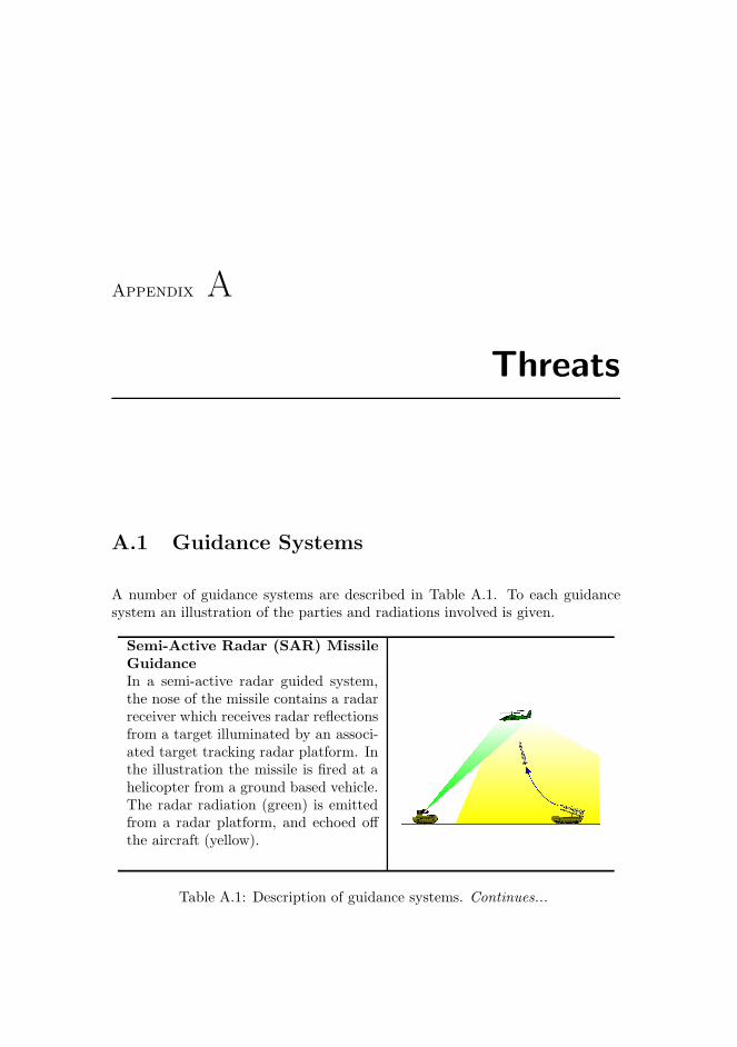
Appendix A
Threats
A.1 Guidance Systems
A number of guidance systems are described in Table A.1. To each guidancesystem an illustration of the parties and radiations involved is given.
Semi-Active Radar (SAR) MissileGuidanceIn a semi-active radar guided system,the nose of the missile contains a radarreceiver which receives radar reflectionsfrom a target illuminated by an associ-ated target tracking radar platform. Inthe illustration the missile is fired at ahelicopter from a ground based vehicle.The radar radiation (green) is emittedfrom a radar platform, and echoed offthe aircraft (yellow).
Table A.1: Description of guidance systems. Continues...
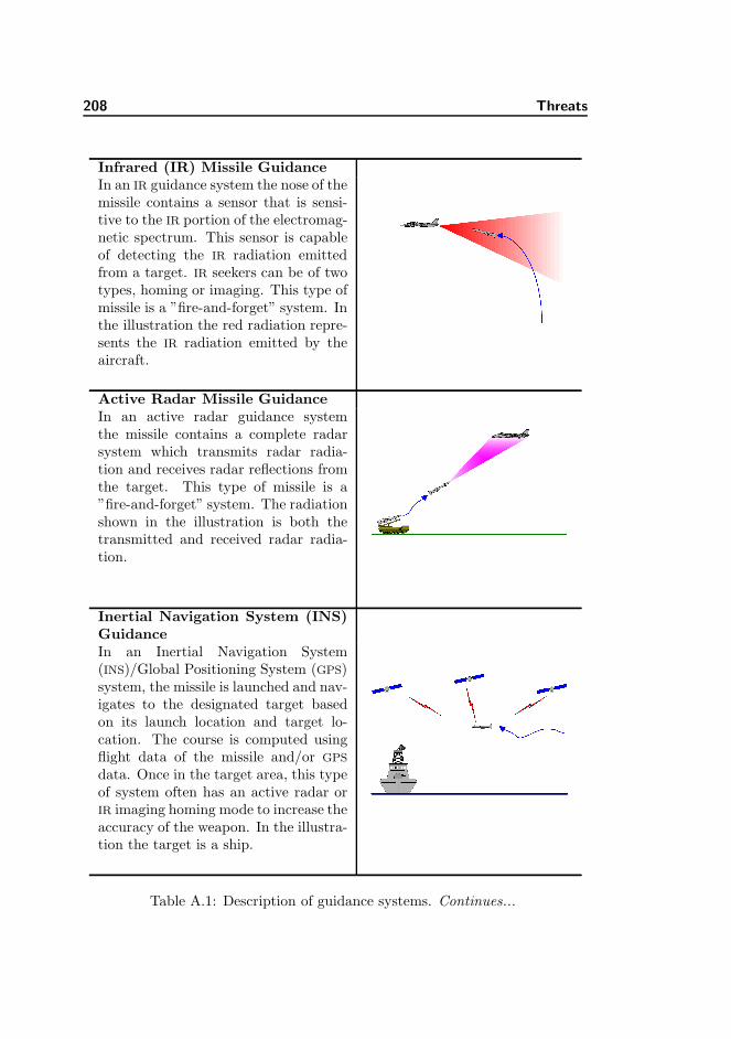
208 Threats
Infrared (IR) Missile GuidanceIn an IR guidance system the nose of themissile contains a sensor that is sensi-tive to the IR portion of the electromag-netic spectrum. This sensor is capableof detecting the IR radiation emittedfrom a target. IR seekers can be of twotypes, homing or imaging. This type ofmissile is a ”fire-and-forget” system. Inthe illustration the red radiation repre-sents the IR radiation emitted by theaircraft.
Active Radar Missile GuidanceIn an active radar guidance systemthe missile contains a complete radarsystem which transmits radar radia-tion and receives radar reflections fromthe target. This type of missile is a”fire-and-forget” system. The radiationshown in the illustration is both thetransmitted and received radar radia-tion.
Inertial Navigation System (INS)GuidanceIn an Inertial Navigation System(INS)/Global Positioning System (GPS)system, the missile is launched and nav-igates to the designated target basedon its launch location and target lo-cation. The course is computed usingflight data of the missile and/or GPS
data. Once in the target area, this typeof system often has an active radar orIR imaging homing mode to increase theaccuracy of the weapon. In the illustra-tion the target is a ship.
Table A.1: Description of guidance systems. Continues...
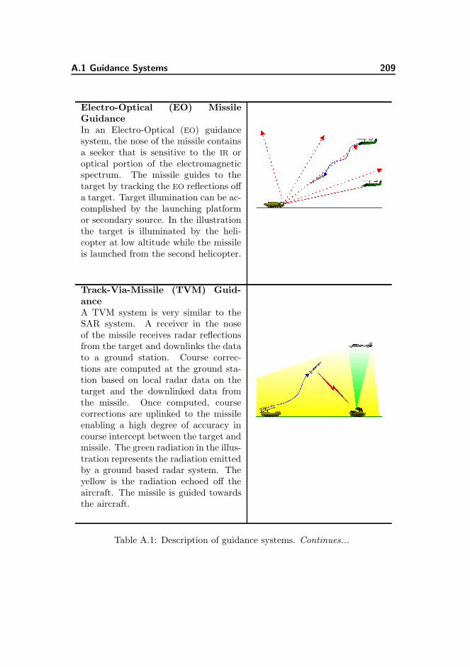
A.1 Guidance Systems 209
Electro-Optical (EO) MissileGuidanceIn an Electro-Optical (EO) guidancesystem, the nose of the missile containsa seeker that is sensitive to the IR oroptical portion of the electromagneticspectrum. The missile guides to thetarget by tracking the EO reflections offa target. Target illumination can be ac-complished by the launching platformor secondary source. In the illustrationthe target is illuminated by the heli-copter at low altitude while the missileis launched from the second helicopter.
Track-Via-Missile (TVM) Guid-anceA TVM system is very similar to theSAR system. A receiver in the noseof the missile receives radar reflectionsfrom the target and downlinks the datato a ground station. Course correc-tions are computed at the ground sta-tion based on local radar data on thetarget and the downlinked data fromthe missile. Once computed, coursecorrections are uplinked to the missileenabling a high degree of accuracy incourse intercept between the target andmissile. The green radiation in the illus-tration represents the radiation emittedby a ground based radar system. Theyellow is the radiation echoed off theaircraft. The missile is guided towardsthe aircraft.
Table A.1: Description of guidance systems. Continues...
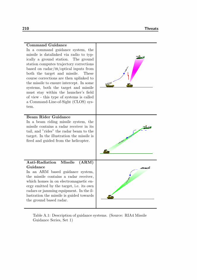
210 Threats
Command GuidanceIn a command guidance system, themissile is datalinked via radio to typ-ically a ground station. The groundstation computes trajectory correctionsbased on radar/IR/optical inputs fromboth the target and missile. Thesecourse corrections are then uplinked tothe missile to ensure intercept. In somesystems, both the target and missilemust stay within the launcher’s fieldof view - this type of systems is calleda Command-Line-of-Sight (CLOS) sys-tem.
Beam Rider GuidanceIn a beam riding missile system, themissile contains a radar receiver in itstail, and ”rides” the radar beam to thetarget. In the illustration the missile isfired and guided from the helicopter.
Anti-Radiation Missile (ARM)GuidanceIn an ARM based guidance system,the missile contains a radar receiver,which homes in on electromagnetic en-ergy emitted by the target, i.e. its ownradars or jamming equipment. In the il-lustration the missile is guided towardsthe ground based radar.
Table A.1: Description of guidance systems. (Source: RIA4 MissileGuidance Series, Set 1)
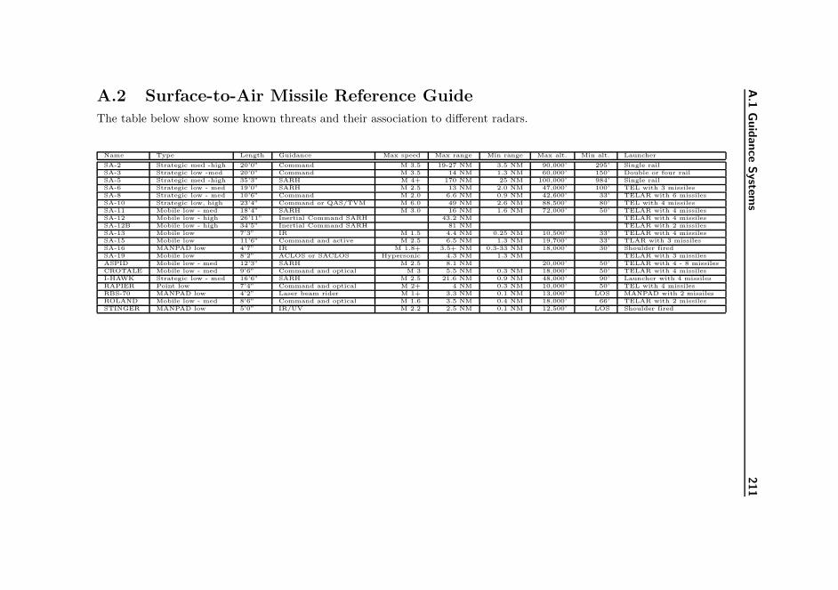
A.1
Guid
ance
Syste
ms
211
A.2 Surface-to-Air Missile Reference Guide
The table below show some known threats and their association to different radars.
Name Type Length Guidance Max speed Max range Min range Max alt. Min alt. Launcher
SA-2 Strategic med -high 20’0” Command M 3.5 19-27 NM 3.5 NM 90,000’ 295’ Single rail
SA-3 Strategic low -med 20’0” Command M 3.5 14 NM 1.3 NM 60,000’ 150’ Double or four rail
SA-5 Strategic med -high 35’3” SARH M 4+ 170 NM 25 NM 100,000’ 984’ Single rail
SA-6 Strategic low - med 19’0” SARH M 2.5 13 NM 2.0 NM 47,000’ 100’ TEL with 3 missiles
SA-8 Strategic low - med 10’6” Command M 2.0 6.6 NM 0.9 NM 42,600’ 33’ TELAR with 6 missiles
SA-10 Strategic low, high 23’4” Command or QAS/TVM M 6.0 49 NM 2.6 NM 88,500’ 80’ TEL with 4 missiles
SA-11 Mobile low - med 18’4” SARH M 3.0 16 NM 1.6 NM 72,000’ 50’ TELAR with 4 missiles
SA-12 Mobile low - high 26’11” Inertial Command SARH 43.2 NM TELAR with 4 missiles
SA-12B Mobile low - high 34’5” Inertial Command SARH 81 NM TELAR with 2 missiles
SA-13 Mobile low 7’3” IR M 1.5 4.4 NM 0.25 NM 10,500’ 33’ TELAR with 4 missiles
SA-15 Mobile low 11’6” Command and active M 2.5 6.5 NM 1.3 NM 19,700’ 33’ TLAR with 3 missiles
SA-16 MANPAD low 4’7” IR M 1.8+ 3.5+ NM 0.3-33 NM 18,000’ 30’ Shoulder fired
SA-19 Mobile low 8’2” ACLOS or SACLOS Hypersonic 4.3 NM 1.3 NM TELAR with 3 missiles
ASPID Mobile low - med 12’3” SARH M 2.5 8.1 NM 20,000’ 50’ TELAR with 4 - 8 missiles
CROTALE Mobile low - med 9’6” Command and optical M 3 5.5 NM 0.3 NM 18,000’ 50’ TELAR with 4 missiles
I-HAWK Strategic low - med 16’6” SARH M 2.5 21.6 NM 0.9 NM 48,000’ 90’ Launcher with 4 missiles
RAPIER Point low 7’4” Command and optical M 2+ 4 NM 0.3 NM 10,000’ 50’ TEL with 4 missiles
RBS-70 MANPAD low 4’2” Laser beam rider M 1+ 3.3 NM 0.1 NM 13,000’ LOS MANPAD with 2 missiles
ROLAND Mobile low - med 8’6” Command and optical M 1.6 3.5 NM 0.4 NM 18,000’ 66’ TELAR with 2 missiles
STINGER MANPAD low 5’0” IR/UV M 2.2 2.5 NM 0.1 NM 12,500’ LOS Shoulder fired

212 Threats
Appendix B
The Prolog Program
B.1 Rules
1. Probable threats are determined pre-mission.
2. Environment hostility depends on the number of anticipated threats.
3. Number of anticipated threats is based on intelligence.
4. A transport aircraft experience hostile environment during take-off andlanding.
5. Data is collected real-time via datalink and warning systems.
6. The breaklock zones for chaff are at 4 o’clock and at 8 o’clock.
7. In case of a missile warning there is no time to deploy the towed decoy.
8. Dispense chaff and flares only when the distance to the threat is right.
9. For chaff the distance to the threat should be less than 5 km and morethan 500 m.
10. If flares are to be used reactively, the distance to the threat should be lessthan 1 km and more than 100 m.

214 The Prolog Program
11. If flares are to be used pre-emptively they should be dispensed as soon aspossible, regardless of any distance.
12. Flares are to be used if the aircraft is in very hostile environment andflying in an altitude below 1000 m.
13. Chaff has no effect against a Doppler radar. Use the jammer instead.
14. At altitudes above 20,000 ft MANPADS is not posing a threat. Use onlychaff.
15. At altitudes below 1,000 ft RF guided missiles are not posing a threat.
16. Chaff and flares can be used as responses to missile warnings.
17. For timing issues jammer and towed decoy can not be used as responsesto warnings, unless they are already in use.
18. If the MWS indicates a missile in a given direction, and the RWR does not,the missile is IR guided.
19. Dispense flares if an approaching missile is IR guided.
20. If both the MWS and the RWR indicate a missile in a given direction, themissile is RF guided.
21. Dispense chaff if an approaching missile is RF guided.
22. If a missile is approaching select the proper countermeasure and manoeu-vre.
23. Manoeuvres are determined by the breaklock zones of the proper counter-measure.
24. The plumes from other aircraft, e.g. wingman and coalition forces, maycause false alarms by the MWS.
25. The positions of other aircraft may be continuously updated, e.g. viadatalink.
26. When the jammer is in ’auto’ mode, it will jam the RF sources detected.
27. Jamming will not commence before the power of the RF source is abovedetection level.
28. The jammer mode is set to ’auto’ when the aircraft fly over hostile envi-ronment.
29. When the jammer is jamming it may influence the RWR and jammers ofother aircraft.
B.2 dss.pro 215
30. The jammer will reveal the position of the aircraft.
31. When flying at high altitudes, the surrounding air is thinner than whenflying at low altitudes.
32. To maintain the effect of flares, when flying in thin air, the amount offlares should be increased.
33. Chaff and flare programs depend on the remaining amount of chaff andflares.
34. Chaff and flare programs depend on the estimated TTG.
35. Flare programs depend on the type of an approaching missile and thealtitude.
36. The types of missiles to anticipate depend on intelligence, and are givenas pre-mission support.
37. The jammer and the towed decoy should not be used simultaneously, un-less they cover different threats.
38. The use of a towed decoy may limit the aircraft manoeuvrability.
39. The RF countermeasure to use may depend on table lookups.
40. The MWS can not distinguish between different types of IR threats
B.2 dss.pro
%−−−−−−−−−−−−−−−−−% Inc lude a d d i t i o n a l f i l e s .%−−−−−−−−−−−−−−−−−:− i n c lude ( ’ t h r e a t s . pro ’ ) .:− i n c lude ( ’cm . pro ’ ) .:− i n c lude ( ’ miss ion . pro ’ ) .:− i n c lude ( ’ cu r r en t . pro ’ ) .:− i n c lude ( ’ warnings . pro ’ ) .:− i n c lude ( ’ u t i l . pro ’ ) .
%−−−−−−−−−−−−−−−−−% The main entry . ’ go ’ w i l l r e turn the t o t a l execu t i on time ,% measured in mi l i s econds .%−−−−−−−−−−−−−−−−−go :−
s ta t i s t i c s ( runtime , [ S tar t | ] ) ,
216 The Prolog Program
what to do ,s ta t i s t i c s ( runtime , [ End | ] ) ,T i s End−Start ,nl , write ( ’ Execution time i s ’ ) ,write (T) , write ( ’ m i l l i s e c on d s ’ ) , nl .
%−−−−−−−−−−−−−−−−−% Warnings are handled and responses to the environment are
found .%−−−−−−−−−−−−−−−−−what to do :−
%−−− Handle warnings(
s e t o f ( ( Warner , WarnInfo ) , warning (Warner , WarnInfo ) ,Warnings ) ,
s e t o f ( , ( memberof (W, Warnings ) , handle warning (W) ) ,) , !
;true
) ,
%−−− Environment responses(
ir mode ( preemptive ) ,a l t i t u d e ( Alt ) ,Alt < 6000 ,(
a v a i l a b l e ( f l a r e s ) ,not ( cm has e f f e c t ( f l a r e s ) ) ,write cm ( f l a r e s , f l a r e s d e f ) , !;a v a i l a b l e ( dircm ) ,not ( cm has e f f e c t ( dircm ) ) ,write cm ( dircm , auto ) , !
);true
) , (r f h o s t i l i t y ( high ) ,a l t i t u d e ( Alt ) ,Alt > 300 ,(
cm has e f f e c t ( jammer ) , !;cm has e f f e c t ( towed decoy ) , !;
B.2 dss.pro 217
cm has e f f e c t ( cha f f ) , !;a v a i l a b l e ( jammer ) ,write cm ( jammer , auto ) , !;a v a i l a b l e ( towed decoy ) ,write cm ( towed decoy , auto ) , !;a v a i l a b l e ( cha f f ) ,write cm ( cha f f , c h a f f d e f ) , !
);true
) .
%−−−−−−−−−−−−−−−−−% Find ac t i on s to each warning , and wr i te them to the screen .%−−−−−−−−−−−−−−−−−handle warning ( ( Sensor , ( Angle , WarnData ) ) ) :−
(Sensor = rwr;Sensor = mws,not ( f r i e n d ( Angle ) )
) ,recommend action ( ( Sensor , ( Angle , WarnData ) ) , Cm, Man,
Prog ) ,
%−−− Write r e s u l t swr i t e t h r e a t ( ( Sensor , ( Angle , WarnData ) ) ) ,write manoeuvre (Man) ,write cm (Cm, Prog ) .
%−−−−−−−−−−−−−−−−−% Recommend ac t i on ( countermeasure , manoeuvre , and programme)%−−−−−−−−−−−−−−−−−recommend action (Warning , Cm, Man, Prog ) :−
recommend cm(Warning , Cm) ,recommend man (Warning , Cm, Man) ,prog (Cm, Prog ) .
%−−−−−−−−−−−−−−−−−% Which countermeasures shou l d be recommended to m i t i g a t e% t h r e a t s at Angle?
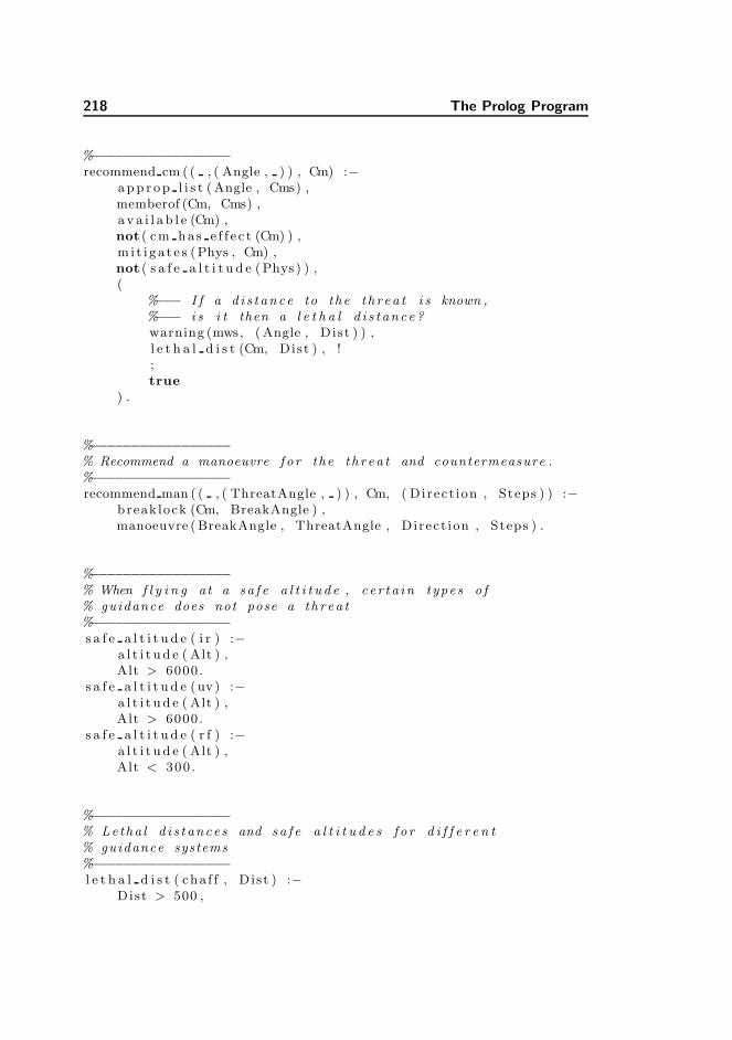
218 The Prolog Program
%−−−−−−−−−−−−−−−−−recommend cm ( ( , ( Angle , ) ) , Cm) :−
app r op l i s t ( Angle , Cms) ,memberof (Cm, Cms) ,a v a i l a b l e (Cm) ,not ( cm has e f f e c t (Cm) ) ,m i t i ga t e s (Phys , Cm) ,not ( s a f e a l t i t u d e (Phys ) ) ,(
%−−− I f a d i s t ance to the t h r ea t i s known ,%−−− i s i t then a l e t h a l d i s t ance ?warning (mws, ( Angle , Dist ) ) ,l e t h a l d i s t (Cm, Dist ) , !;true
) .
%−−−−−−−−−−−−−−−−−% Recommend a manoeuvre f o r the t h r ea t and countermeasure .%−−−−−−−−−−−−−−−−−recommend man ( ( , ( ThreatAngle , ) ) , Cm, ( Direct ion , Steps ) ) :−
break lock (Cm, BreakAngle ) ,manoeuvre ( BreakAngle , ThreatAngle , Direct ion , Steps ) .
%−−−−−−−−−−−−−−−−−% When f l y i n g at a sa f e a l t i t u d e , c e r t a i n types o f% guidance does not pose a th r ea t%−−−−−−−−−−−−−−−−−s a f e a l t i t u d e ( i r ) :−
a l t i t u d e ( Alt ) ,Alt > 6000.
s a f e a l t i t u d e (uv ) :−a l t i t u d e ( Alt ) ,Alt > 6000.
s a f e a l t i t u d e ( r f ) :−a l t i t u d e ( Alt ) ,Alt < 300 .
%−−−−−−−−−−−−−−−−−% Letha l d i s t ance s and sa f e a l t i t u d e s f o r d i f f e r e n t% guidance systems%−−−−−−−−−−−−−−−−−l e t h a l d i s t ( cha f f , Dist ) :−
Dist > 500 ,
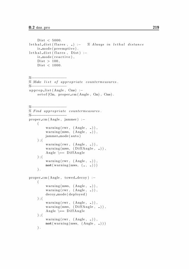
B.2 dss.pro 219
Dist < 5000.l e t h a l d i s t ( f l a r e s , ) :− % Always in l e t h a l d i s t ance
ir mode ( preemptive ) .l e t h a l d i s t ( f l a r e s , Dist ) :−
ir mode ( r e a c t i v e ) ,Dist > 100 ,Dist < 1000.
%−−−−−−−−−−−−−−−−−% Make l i s t o f appropr i a te countermeasures .%−−−−−−−−−−−−−−−−−app r op l i s t ( Angle , Cms) :−
s e t o f (Cm, proper cm ( Angle , Cm) , Cms) .
%−−−−−−−−−−−−−−−−−% Find appropr i a te countermeasures .%−−−−−−−−−−−−−−−−−proper cm ( Angle , jammer ) :−
(warning ( rwr , ( Angle , ) ) ,warning (mws, ( Angle , ) ) ,jammer mode ( auto )
) ; (warning ( rwr , ( Angle , ) ) ,warning (mws, ( Di f fAngle , ) ) ,Angle \== Dif fAngle
) ; (warning ( rwr , ( Angle , ) ) ,not ( warning (mws, ( , ) ) )
) .
proper cm ( Angle , towed decoy ) :−(
warning (mws, ( Angle , ) ) ,warning ( rwr , ( Angle , ) ) ,decoy mode ( deployed )
) ; (warning ( rwr , ( Angle , ) ) ,warning (mws, ( Di f fAngle , ) ) ,Angle \== Dif fAngle
) ; (warning ( rwr , ( Angle , ) ) ,not ( warning (mws, ( Angle , ) ) )
) .
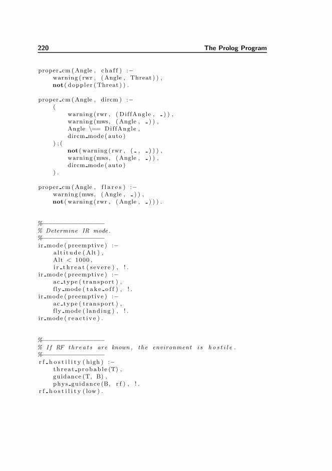
220 The Prolog Program
proper cm ( Angle , ch a f f ) :−warning ( rwr , ( Angle , Threat ) ) ,not ( doppler ( Threat ) ) .
proper cm ( Angle , dircm ) :−(
warning ( rwr , ( Di f fAngle , ) ) ,warning (mws, ( Angle , ) ) ,Angle \== Dif fAngle ,dircm mode ( auto )
) ; (not ( warning ( rwr , ( , ) ) ) ,warning (mws, ( Angle , ) ) ,dircm mode ( auto )
) .
proper cm ( Angle , f l a r e s ) :−warning (mws, ( Angle , ) ) ,not ( warning ( rwr , ( Angle , ) ) ) .
%−−−−−−−−−−−−−−−−−% Determine IR mode .%−−−−−−−−−−−−−−−−−ir mode ( preemptive ) :−
a l t i t u d e ( Alt ) ,Alt < 1000 ,i r t h r e a t ( seve re ) , ! .
ir mode ( preemptive ) :−ac type ( t ran spor t ) ,f ly mode ( t a k e o f f ) , ! .
ir mode ( preemptive ) :−ac type ( t ran spor t ) ,f ly mode ( land ing ) , ! .
ir mode ( r e a c t i v e ) .
%−−−−−−−−−−−−−−−−−% I f RF t h r e a t s are known , the environment i s h o s t i l e .%−−−−−−−−−−−−−−−−−r f h o s t i l i t y ( high ) :−
t h r e a t p r obab l e (T) ,guidance (T, B) ,phys gu idance (B, r f ) , ! .
r f h o s t i l i t y ( low ) .
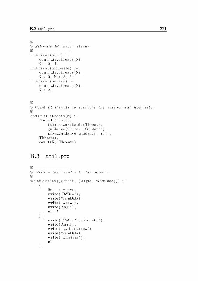
B.3 util.pro 221
%−−−−−−−−−−−−−−−−−% Estimate IR th r ea t s t a t u s .%−−−−−−−−−−−−−−−−−i r t h r e a t ( none ) :−
c ou n t i r t h r e a t s (N) ,N = 0 , ! .
i r t h r e a t ( moderate ) :−c ou n t i r t h r e a t s (N) ,N > 0 , N < 3 , ! .
i r t h r e a t ( seve re ) :−c ou n t i r t h r e a t s (N) ,N > 2 .
%−−−−−−−−−−−−−−−−−% Count IR t h r e a t s to es t imate the environment h o s t i l i t y .%−−−−−−−−−−−−−−−−−c ou n t i r t h r e a t s (N) :−
f indal l ( Threat ,( t h r e a t p r obab l e ( Threat ) ,guidance ( Threat , Guidance ) ,phys gu idance ( Guidance , i r ) ) ,
Threats ) ,count (N, Threats ) .
B.3 util.pro
%−−−−−−−−−−−−−−−−−% Writing the r e s u l t s to the screen .%−−−−−−−−−−−−−−−−−wr i t e t h r e a t ( ( Sensor , ( Angle , WarnData ) ) ) :−
(Sensor = rwr ,write ( ’RWR: ’ ) ,write (WarnData ) ,write ( ’ at ’ ) ,write ( Angle ) ,nl , !
) ; (write ( ’MWS: M i s s i l e at ’ ) ,write ( Angle ) ,write ( ’ , d i s t an c e ’ ) ,write (WarnData ) ,write ( ’ meters ’ ) ,nl
) .
222 The Prolog Program
write manoeuvre ( ( Direct ion , Steps ) ) :−(
Steps == 0 ,write ( ’ Stay on cour se ’ ) ,nl , !
) ; (write ( ’Turn ’ ) ,write ( D i r ec t ion ) ,write ( ’ , ’ ) ,write ( Steps ) ,write ( ’ s tep ( s ) ’ ) ,nl
) .
write cm (Cm, Prog ) :−write ( ’Use ’ ) ,write (Cm) ,write ( ’ , program ’ ) ,write ( Prog ) ,nl ,nl .
%−−−−−−−−−−−−−−−−−% Angles .%−−−−−−−−−−−−−−−−−t u rn r i gh t ( one o c lock , two o c lock ) .t u rn r i gh t ( two o c lock , t h r e e o c l o c k ) .t u rn r i gh t ( t h r e e o c l o ck , f o u r o c l o c k ) .t u rn r i gh t ( f ou r o c l o ck , f i v e o c l o c k ) .t u rn r i gh t ( f i v e o c l o c k , s i x o c l o c k ) .t u rn r i gh t ( s i x o c l o c k , s ev en o c l o ck ) .t u rn r i gh t ( seven o c lock , e i g h t o c l o c k ) .t u rn r i gh t ( e i gh t o c l o ck , n i n e o c l o c k ) .t u rn r i gh t ( n in e o c l o ck , t en o c l o ck ) .t u rn r i gh t ( t en o c l o ck , e l e v e n o c l o c k ) .t u rn r i gh t ( e l e v en o c l o ck , twe l v e o c l o ck ) .t u rn r i gh t ( twe lv e o c lock , on e o c l o ck ) .
t u r n l e f t (X, Y) :−t u rn r i gh t (Y, X) .
%−−−−−−−−−−−−−−−−−% Manoeuvres .%−−−−−−−−−−−−−−−−−
B.4 cm.pro 223
manoeuvre l e f t (Same , Same , Steps ) :−Steps i s 0 .
manoeuvre l e f t (From , To , Steps ) :−t u r n l e f t (From , NewAngle ) ,manoeuvre l e f t (NewAngle , To , MoreSteps ) ,Steps i s MoreSteps + 1 .
manoeuvre r ight (Same , Same , Steps ) :−Steps i s 0 .
manoeuvre r ight (From , To , Steps ) :−t u rn r i gh t (From , NewAngle ) ,manoeuvre r ight (NewAngle , To , MoreSteps ) ,Steps i s MoreSteps + 1 .
manoeuvre (From , To , Direct ion , Steps ) :−manoeuvre l e f t (From , To , S tep sLe f t ) ,manoeuvre r ight (From , To , StepsRight ) ,
( S t ep sLe f t < StepsRight , Steps i s StepsLeft , D i r ec t ion =l e f t , ! ;
Steps i s StepsRight , D i r ec t ion = r igh t , ! ) .
%−−−−−−−−−−−−−−−−−% Li s t f unc t i on s .%−−−−−−−−−−−−−−−−−%−−− Number o f memberscount (0 , [ ] ) :− ! .count (N, [ | Tai l ] ) :−
count (N1 , Ta i l ) ,N i s N1 + 1 .
%−−− Membershipmemberof (X, [X | ] ) .memberof (X, [ | Tai l ] ) :− memberof (X, Ta i l ) .
B.4 cm.pro
%−−−−−−−−−−−−−−−−−% Break−l o c k zones%−−−−−−−−−−−−−−−−−break lock ( cha f f , f o u r o c l o c k ) .break lock ( cha f f , e i g h t o c l o c k ) .break lock ( jammer , on e o c l o ck ) .break lock ( jammer , f i v e o c l o c k ) .break lock ( jammer , s i x o c l o c k ) .break lock ( jammer , s ev en o c l o ck ) .
224 The Prolog Program
break lock ( jammer , e l e v e n o c l o c k ) .break lock ( jammer , twe l v e o c l o ck ) .break lock (Cm, ) :−
(Cm = chaf f , ! , f a i l ) ;(Cm = jammer , ! , f a i l ) ;true .
%−−−−−−−−−−−−−−−−−% Countermeasure programs%−−−−−−−−−−−−−−−−−%−−− Flare programs
prog ( f l a r e s , f l a r e s 0 1 ) :−f l a r e s l e f t (FL) ,FL > 5 ,a l t i t u d e ( Alt ) ,Alt < 300 , ! .
prog ( f l a r e s , f l a r e s 0 2 ) :−f l a r e s l e f t (FL) ,FL > 7 ,a l t i t u d e ( Alt ) ,Alt < 500 , ! .
prog ( f l a r e s , f l a r e s d e f ) :−f l a r e s l e f t (FL) ,FL > 7 , ! .
prog ( f l a r e s , none ) :− f a i l , ! .
%−−− Chaff programsprog ( cha f f , cha f f01 ) :−
c h a f f l e f t (CL) ,CL > 6 ,a l t i t u d e ( Alt ) ,Alt < 500 ,warning ( rwr , ( , sa2 ) ) , ! .
prog ( cha f f , cha f f01 ) :−c h a f f l e f t (CL) ,CL > 6 ,a l t i t u d e ( Alt ) ,Alt < 1000 ,warning ( rwr , ( , sa6 ) ) , ! .
prog ( cha f f , c h a f f d e f ) :−
B.5 threats.pro 225
c h a f f l e f t (CL) ,CL > 5 , ! .
prog ( cha f f , ) :− f a i l , ! .
%−−− Defau l t ( at the end )prog ( , d e f au l t ) .
%−−−−−−−−−−−−−−−−−% Are the countermeasures cu r r en t l y m i t i g a t i n g ?%−−−−−−−−−−−−−−−−−cm has e f f e c t ( towed decoy ) :−
decoy mode ( deployed ) .
cm has e f f e c t ( jammer ) :−jammer mode ( auto ) .
cm has e f f e c t ( dircm ) :−dircm mode ( auto ) .
cm has e f f e c t ( cha f f ) :−c h a f f d i s p (Time) ,Time < 3 .
cm has e f f e c t ( f l a r e s ) :−f l a r e s d i s p (Time) ,Time < 1 .
B.5 threats.pro
%−−−−−−−−−−−−−−−−−% Mi s s i l e systems%−−−−−−−−−−−−−−−−−guidance ( sa2 , command) .guidance ( sa3 , command) .guidance ( sa5 , sarh ) . % Dopplerguidance ( sa6 , sarh ) .guidance ( sa8 , command) .guidance ( sa10 , command) . % Dopplerguidance ( sa10 , qas tvm ) .guidance ( sa11 , sarh ) .guidance ( sa12 , i n e r t i a l ) .guidance ( sa12 , command) .guidance ( sa12 , sarh ) .guidance ( sa12b , i n e r t i a l ) .
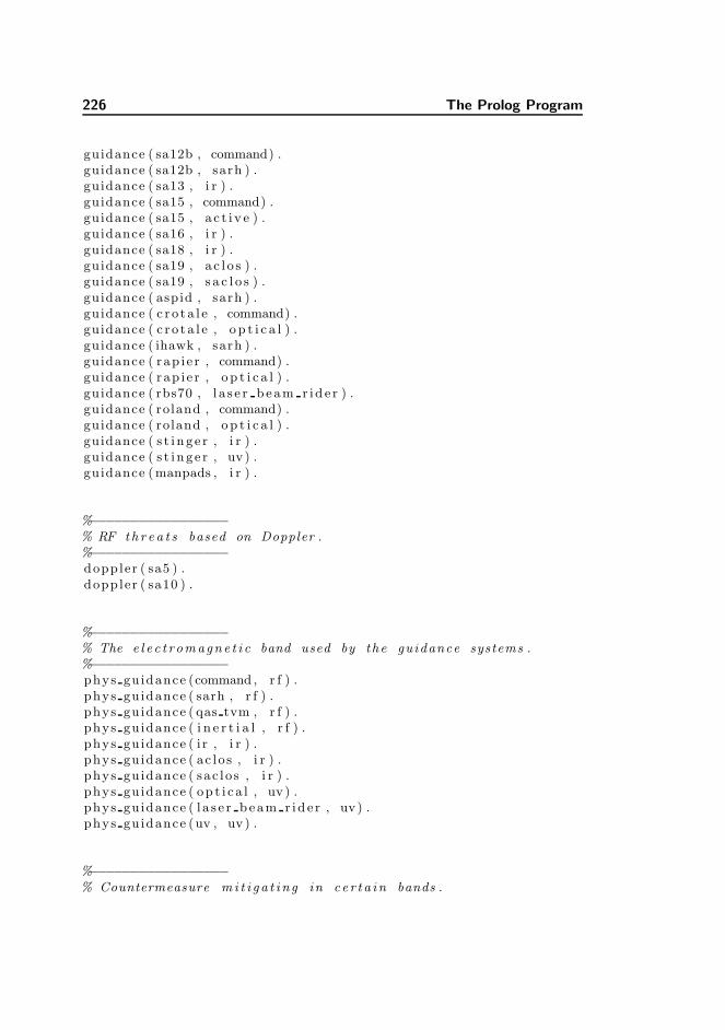
226 The Prolog Program
guidance ( sa12b , command) .guidance ( sa12b , sarh ) .guidance ( sa13 , i r ) .guidance ( sa15 , command) .guidance ( sa15 , a c t i v e ) .guidance ( sa16 , i r ) .guidance ( sa18 , i r ) .guidance ( sa19 , a c l o s ) .guidance ( sa19 , s a c l o s ) .guidance ( aspid , sarh ) .guidance ( c r o t a l e , command) .guidance ( c r o t a l e , o p t i c a l ) .guidance ( ihawk , sarh ) .guidance ( rap i e r , command) .guidance ( rap i e r , o p t i c a l ) .guidance ( rbs70 , l a s e r b eam r id e r ) .guidance ( roland , command) .guidance ( roland , o p t i c a l ) .guidance ( s t i n g e r , i r ) .guidance ( s t i n g e r , uv ) .guidance (manpads , i r ) .
%−−−−−−−−−−−−−−−−−% RF th r e a t s based on Doppler .%−−−−−−−−−−−−−−−−−doppler ( sa5 ) .doppler ( sa10 ) .
%−−−−−−−−−−−−−−−−−% The e l e c t r omagne t i c band used by the guidance systems .%−−−−−−−−−−−−−−−−−phys gu idance (command , r f ) .phys gu idance ( sarh , r f ) .phys gu idance ( qas tvm , r f ) .phys gu idance ( i n e r t i a l , r f ) .phys gu idance ( i r , i r ) .phys gu idance ( ac lo s , i r ) .phys gu idance ( sac lo s , i r ) .phys gu idance ( op t i c a l , uv ) .phys gu idance ( l a s e r b eam r id e r , uv ) .phys gu idance (uv , uv ) .
%−−−−−−−−−−−−−−−−−% Countermeasure m i t i g a t i n g in c e r t a i n bands .
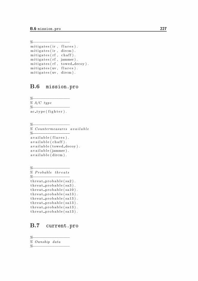
B.6 mission.pro 227
%−−−−−−−−−−−−−−−−−mit i ga t e s ( i r , f l a r e s ) .m i t i ga t e s ( i r , dircm ) .m i t i ga t e s ( r f , c h a f f ) .m i t i ga t e s ( r f , jammer ) .m i t i ga t e s ( r f , towed decoy ) .m i t i ga t e s (uv , f l a r e s ) .m i t i ga t e s (uv , dircm ) .
B.6 mission.pro
%−−−−−−−−−−−−−−−−−% A/C type%−−−−−−−−−−−−−−−−−ac type ( f i g h t e r ) .
%−−−−−−−−−−−−−−−−−% Countermeasures a v a i l a b l e%−−−−−−−−−−−−−−−−−av a i l a b l e ( f l a r e s ) .a v a i l a b l e ( cha f f ) .a v a i l a b l e ( towed decoy ) .a v a i l a b l e ( jammer ) .a v a i l a b l e ( dircm ) .
%−−−−−−−−−−−−−−−−−% Probab le t h r e a t s%−−−−−−−−−−−−−−−−−t h r e a t p r obab l e ( sa2 ) .t h r e a t p r obab l e ( sa3 ) .t h r e a t p r obab l e ( sa10 ) .t h r e a t p r obab l e ( sa13 ) .t h r e a t p r obab l e ( sa13 ) .t h r e a t p r obab l e ( sa13 ) .t h r e a t p r obab l e ( sa13 ) .t h r e a t p r obab l e ( sa13 ) .
B.7 current.pro
%−−−−−−−−−−−−−−−−−% Ownship data%−−−−−−−−−−−−−−−−−
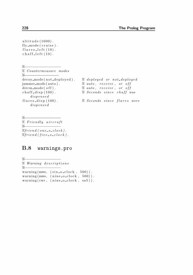
228 The Prolog Program
a l t i t u d e (1600) .f ly mode ( c r u i s e ) .f l a r e s l e f t ( 10) .c h a f f l e f t ( 10) .
%−−−−−−−−−−−−−−−−−% Countermeasure modes%−−−−−−−−−−−−−−−−decoy mode ( not dep loyed ) . % deployed or no t dep l oyedjammer mode ( auto ) . % auto , rece i ve , or o f fdircm mode ( o f f ) . % auto , rece i ve , or o f fc h a f f d i s p (100) . % Seconds s ince c h a f f was
d i spensedf l a r e s d i s p (100) . % Seconds s ince f l a r e s were
d i spensed
%−−−−−−−−−−−−−−−−−% Fri end l y a i r c r a f t%−−−−−−−−−−−−−−−−−%f r i end ( one o c l o c k ) .%f r i end ( f i v e o c l o c k ) .
B.8 warnings.pro
%−−−−−−−−−−−−−−−−−% Warning d e s c r i p t i o n s%−−−−−−−−−−−−−−−−−warning (mws, ( s i x o c l o c k , 500) ) .warning (mws, ( n in e o c l o ck , 500) ) .warning ( rwr , ( n in e o c l o ck , sa5 ) ) .
Appendix C
Survival Score
C.1 Constructing a score system
In medicine score systems like Glasgow Coma Score [50] and Apgar Score [8] areused to give the medical staff a fast overview of the conditions of a patient. Theadvantage of score systems is that they will get this overview without the labourand time it will take to do a more detailed examination. The score systems areoften used to make decisions on the treatment of the patient when there is notime to do more examinations. A score may include scores from other scoresystems.
Constructing a score system for the survivability of a fighter aircraft has muchthe same use as a medical score system. A higher score indicates a highersurvivability for the aircraft. Optimising the score is another way of givingthe aircraft the best chances of surviving. A difference is the use of simplicity:a medical score is often fast calculated by the medical staff based on a fewobservations, and without any tools for doing the calculations. It thereforehas to be relatively simple and easy to calculate. The survival score can becalculated with more complex parts since it will be calculated automatically.

230 Survival Score
C.1.1 Contributions to the score
The list below shows some of the aspects to be taken into account when calcu-lating a survival score:
1. Threats contribute with a negative value. Probability of the threat is usedfor weighing the value.
2. Multiple threats increase the threat value. The increase is not proportionalto the number of threats since applied countermeasures may influence morethan one threat.
3. Applying proper countermeasures should add a positive number of thesame magnitude as that of the threat being treated. Difference betweencurrent aspect angle and the preferred angle is used as weight.
4. The score can have a temporal aspect, depending on the recent history.If proper countermeasures have already been applied, and the effect ofthese has not yet been registered, the threat contributes with a numericalsmaller value.
5. The score may also depend on the remaining amount of chaff and flares.Having the possibility of using a proper countermeasure adds one value,actually using it adds another.
6. Using the wrong countermeasure adds a penalty value, since this mightdecrease the survivability later on in the mission.
7. The probability of emerging threats, depending on e.g. the territory, willalso have an influence on the score. This may make the altitude relevant.
Some of the contributing parts do not need to be included every time the scoreis calculated. An example of this is the part concerning the altitude. Changingthe altitude is a relatively slow process, and even though a change in altitudeis in progress it is fair to assume that this part should not be considered moreoften than once every two seconds or even more infrequently.
C.2 Optimising the score 231
C.1.2 Formalizing the score
S The survivability scoreK = {IR, RF, ...} The domains of threat to considerP (k), k ∈ K The probability of a threat k. Depends on sensor outputak ∈ {0, 1} The applicability of the score from the k’th domainsk Score for the k’th domainLk ∈ {0, 1} Countermeasures loaded/presentP (Ak) The probability of the countermeasure being appliedP (Wk) The probability of the countermeasure working as intendedTk ∈ R− Maximal threat valueCk ∈ R+ Maximal countermeasure valuepk(t) The penalty for using countermeasures at time t
The survivability score can be calculated as:
S =Xk∈K
ak · sk (C.1)
sk = −P (k) · Tk (C.2)
+Lk · P (Ak) · P (Wk) · Ck (C.3)
−pk(t) · P (Ak) (C.4)
In the above (C.2) is the threat part of the survival score, (C.3) is the counter-measure part, and (C.4) is the penalty part.
C.2 Optimising the score
Let us rewrite the equation (C.2) – (C.4) as:
sk = −Tk + Ck − Pk (C.5)
It is obvious from equation (C.5) that the maximum value for sk is found whenthe threat part (Tk) and the penalty (Pk) are small and when the countermeasure(Ck) is high. Of these the pilot can only directly influence the countermeasureand penalty parts. If no threat is present the penalty part should have a valuenumerical larger than that of the countermeasure part.

232 Survival Score
Tk = 0⇒ Pk > Ck
Tk 6= 0⇒ Pk � Tk
C.3 Further work
In deciding on the formulation of the survival score one must consider the fol-lowing:
1. More countermeasures to same kind of threat
2. Threats without countermeasures
3. When is a score system ”good enough”?
4. How bad can a full description be, before it is too bad?
Appendix D
The GAMS Program
D.1 tempasp.gms
∗ use : gams tempasp u1=” f l i g h t . dat”
$eolcom //opt ion i t e r l im = 999999999; // avoid l im i t on i t e r a t i o n sopt ion r e s l im = 86400; // time l im i t f o r s o l v e r in
sec .opt ion optcr = 0 . ; // gap t o l e r an c eopt ion s o l p r i n t = ON; // inc lude s o l u t i o n p r i n t in
. l s t f i l eopt ion limrow = 100 ; // l im i t number o f rows in
. l s t f i l eopt ion l imco l = 100 ; // l im i t number o f columns in
. l s t f i l e//−−−−−−−−−−−−−−−−−−−−−−−−−−−−−−
////////////////////Sets
cm ’ Countermeasures ’ / ’ jammer ’ , ’ decoy ’ , ’ cha f f ’ ,’noCm’/
ang ’ Angles o f Attack ’ / 0 ∗ 360 /
234 The GAMS Program
d i s t ’ Distances ’ / 0 ∗ 100 /t ’Time steps ’thr ’ Threats ’;
////////////////////Parameters
redAlpha (cm, ang ) ’ Reduction o f l e t h a l i t y ( Alpha ) ’redRho(cm, d i s t ) ’ Reduction o f l e t h a l i t y (Rho) ’flyAng ( t , thr ) ’ Angles during f l i g h t ’f l yD i s t ( t , thr ) ’ Distances during f l i g h t ’l e t h a l i t y ( t , thr ) ’ L e tha l i t y o f t h r e a t s during f l i g h t ’probThreat ( t , thr ) ’ P r obab i l i t y o f threat ’Rjmr( t , thr ) ’ Reduction by jammer ’Rjmra ( t , thr ) ’ . . . angle ’Rjmrd ( t , thr ) ’ . . . d i s tance ’Rdec ( t , thr ) ’ Reduction by decoy ’Rdeca ( t , thr ) ’ . . . angle ’Rdecd ( t , thr ) ’ . . . d i s tance ’Rchf ( t , thr ) ’ Reduction by cha f f ’Rchfa ( t , thr ) ’ . . . angle ’Rchfd ( t , thr ) ’ . . . d i s tance ’minDist ( t , thr ) ’ Distance to th reat ( l e s s than 200) ’;
$ in c lude ” reduct ion s . dat” // Inc lude reduct ion s$ inc lude ”%gams . user1%” // Inc lude angles , d i s tance s , and
l e t h a l i t i e s
///////// Find the reduct ion sa l i a s ( t , t1 ) ;a l i a s ( d i s t , d1 ) ;a l i a s ( ang , a1 ) ;a l i a s ( thr , thr1 ) ;
loop ( t1 ,loop ( thr1 ,
loop (d1 ,i f ( ord ( d1 )−1 = f l yD i s t ( t1 , thr1 ) ,
Rjmrd ( t1 , thr1 ) = redRho ( ’ jammer ’ , d1 )) ;
) ;loop ( a1 ,
i f ( ord ( a1 )−1 = flyAng ( t1 , thr1 ) ,Rjmra ( t1 , thr1 ) = redAlpha ( ’ jammer ’ , a1 )
D.1 tempasp.gms 235
) ;) ;
) ;) ;Rjmr( t , thr ) = Rjmrd ( t , thr ) ∗ Rjmra ( t , thr ) ;
loop ( t1 ,loop ( thr1 ,
loop (d1 ,i f ( ord ( d1 )−1 = f l yD i s t ( t1 , thr1 ) ,
Rdecd ( t1 , thr1 ) = redRho ( ’ decoy ’ , d1 )) ;
) ;loop ( a1 ,
i f ( ord ( a1 )−1 = flyAng ( t1 , thr1 ) ,Rdeca ( t1 , thr1 ) = redAlpha ( ’ decoy ’ , a1 )
) ;) ;
) ;) ;Rdec ( t , thr ) = Rdecd ( t , thr ) ∗ Rdeca ( t , thr ) ;
loop ( t1 ,loop ( thr1 ,
loop (d1 ,i f ( ord ( d1 )−1 = f l yD i s t ( t1 , thr1 ) ,
Rchfd ( t1 , thr1 ) = redRho ( ’ cha f f ’ , d1 )) ;
) ;loop ( a1 ,
i f ( ord ( a1 )−1 = flyAng ( t1 , thr1 ) ,Rchfa ( t1 , thr1 ) = redAlpha ( ’ cha f f ’ , a1 )
) ;) ;
) ;) ;Rchf ( t , thr ) = Rchfd ( t , thr ) ∗ Rchfa ( t , thr ) ;
///////// Find minimum d i s t an c e to th reatminDist ( t1 , thr1 ) = min(199 , f l yD i s t ( t1 , thr1 ) ) ; // Keep
under 200
///////// Find the p robab i l i t y o f a th reatloop ( t1 ,
loop ( thr1 ,
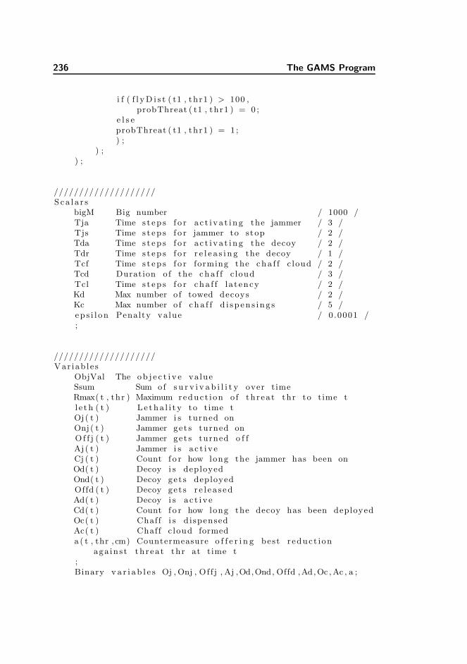
236 The GAMS Program
i f ( f l yD i s t ( t1 , thr1 ) > 100 ,probThreat ( t1 , thr1 ) = 0 ;
e l s eprobThreat ( t1 , thr1 ) = 1 ;) ;
) ;) ;
////////////////////S ca l a r s
bigM Big number / 1000 /Tja Time s t ep s f o r a c t i v a t i n g the jammer / 3 /Tjs Time s t ep s f o r jammer to stop / 2 /Tda Time s t ep s f o r a c t i v a t i n g the decoy / 2 /Tdr Time s t ep s f o r r e l e a s i n g the decoy / 1 /Tcf Time s t ep s f o r forming the cha f f c loud / 2 /Tcd Duration o f the cha f f c loud / 3 /Tcl Time s t ep s f o r cha f f l a t ency / 2 /Kd Max number o f towed decoys / 2 /Kc Max number o f cha f f d i sp en s i n g s / 5 /ep s i l on Penalty value / 0.0001 /;
////////////////////Var iab l e s
ObjVal The ob j e c t i v e valueSsum Sum of s u r v i v a b i l i t y over timeRmax( t , thr ) Maximum reduct ion o f th reat thr to time tl e t h ( t ) Le tha l i t y to time tOj ( t ) Jammer i s turned onOnj ( t ) Jammer get s turned onO f f j ( t ) Jammer get s turned o f fAj ( t ) Jammer i s a c t i v eCj ( t ) Count f o r how long the jammer has been onOd( t ) Decoy i s deployedOnd( t ) Decoy get s deployedOffd ( t ) Decoy get s r e l e a s edAd( t ) Decoy i s a c t i v eCd( t ) Count f o r how long the decoy has been deployedOc( t ) Chaff i s d ispensedAc( t ) Chaff c loud formeda ( t , thr , cm) Countermeasure o f f e r i n g best r educt ion
aga in s t th reat thr at time t;Binary v a r i a b l e s Oj , Onj , Off j , Aj ,Od,Ond, Offd ,Ad,Oc ,Ac , a ;
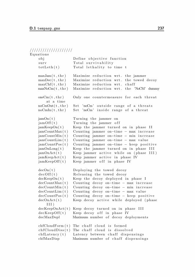
D.1 tempasp.gms 237
////////////////////Equations
obj Def ine ob j e c t i v e funct ionsurv Total s u r v i v a b i l i t ytotLeth ( t ) Total l e t h a l i t y to time t
maxJam( t , thr ) Maximize r educt ion wrt . the jammermaxDec( t , thr ) Maximize r educt ion wrt . the towed decoymaxChf( t , thr ) Maximize r educt ion wrt . ch a f fmaxNoCm( t , thr ) Maximize r educt ion wrt . the ’NoCM’ dummy
oneCm( t , thr ) Only one countermeasure f o r each th reatat a time
noCmOut( t , thr ) Set ’noCm’ out s ide range o f a th r ea t snoCmIn( t , thr ) Set ’noCm’ i n s i d e range o f a th reat
jamOn( t ) Turning the jammer onjamOff ( t ) Turning the jammer o f fjamKeepOn( t ) Keep the jammer turned on in phase I IjamCountMax ( t ) Counting jammer on−time − max in c r e a s ejamCountMin ( t ) Counting jammer on−time − min in c r e a s ejamCountLim ( t ) Counting jammer on−time − max valuejamCountPos ( t ) Counting jammer on−time − keep p o s i t i v ejamOnLong( t ) Keep the jammer turned on in phase I I IjamOnAct ( t ) Keep jammer ac t i v e whi le on ( phase I I I )jamKeepAct ( t ) Keep jammer ac t i v e in phase IVjamKeepOff ( t ) Keep jammer o f f in phase IV
decOn( t ) Deploying the towed decoydecOff ( t ) Re l eas ing the towed decoydecKeepOn( t ) Keep the decoy deployed in phase IdecCountMax ( t ) Counting decoy on−time − max in c r e a s edecCountMin ( t ) Counting decoy on−time − min in c r e a s edecCountLim ( t ) Counting decoy on−time − max valuedecCountPos ( t ) Counting decoy on−time − keep p o s i t i v edecOnAct( t ) Keep decoy ac t i v e whi le deployed ( phase
I I I )decKeepOnAct( t ) Keep decoy turned on in phase I I IdecKeepOff ( t ) Keep decoy o f f in phase IVdecMaxDepl Maximum number o f decoy deployments
chfCloudForm ( t ) The cha f f c loud i s formedchfCloudDiss ( t ) The cha f f c loud i s d i s s o l v edchfLatency ( t ) Latency between cha f f d i sp en s i n g schfMaxDisp Maximum number o f cha f f d i sp en s i n g s
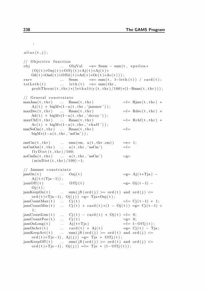
238 The GAMS Program
;
a l i a s ( t , j ) ;
// Object ive funct ionobj . . ObjVal =e= Ssum − sum( t , ep s i l on ∗
(Oj ( t )+Onj ( t )+Of f j ( t )+Aj ( t )+Aj ( t )+Od( t )+Ond( t )+Offd ( t )+Ad( t )+Oc( t )+Ac( t ) ) ) ;
surv . . Ssum =e= sum( t , 1− l e t h ( t ) ) / card ( t ) ;totLeth ( t ) . . l e t h ( t ) =e= sum( thr ,
probThreat ( t , thr ) ∗( l e t h a l i t y ( t , thr ) /100) ∗(1−Rmax( t , thr ) ) ) ;
// General c on s t r a i n t smaxJam( t , thr ) . . Rmax( t , thr ) =l= Rjmr ( t , thr ) ∗
Aj ( t ) + bigM∗(1−a ( t , thr , ’ jammer ’ ) ) ;maxDec( t , thr ) . . Rmax( t , thr ) =l= Rdec ( t , thr ) ∗
Ad( t ) + bigM∗(1−a ( t , thr , ’ decoy ’ ) ) ;maxChf( t , thr ) . . Rmax( t , thr ) =l= Rchf ( t , thr ) ∗
Ac( t ) + bigM∗(1−a ( t , thr , ’ cha f f ’ ) ) ;maxNoCm( t , thr ) . . Rmax( t , thr ) =l=
bigM∗(1−a ( t , thr , ’noCm’ ) ) ;
oneCm( t , thr ) . . sum(cm, a ( t , thr , cm) ) =e= 1 ;noCmOut( t , thr ) . . a ( t , thr , ’noCm’ ) =l=
f l yD i s t ( t , thr ) /100;noCmIn( t , thr ) . . a ( t , thr , ’noCm’ ) =g=
( minDist ( t , thr ) /100) −1;
// Jammer c on s t r a i n t sjamOn( t ) . . Onj ( t ) =g= Aj ( t+Tja ) −
Aj ( t+(Tja−1) ) ;jamOff ( t ) . . O f f j ( t ) =g= Oj ( t−1) −
Oj ( t ) ;jamKeepOn( t ) . . sum( j$ ( ord ( j ) >= ord ( t ) and ord ( j ) <=
ord ( t )+Tja−1) , Oj ( j ) ) =g= Tja∗Onj ( t ) ;jamCountMax( t ) . . Cj ( t ) =l= Cj ( t−1) + 1 ;jamCountMin ( t ) . . Cj ( t ) + card ( t ) ∗(1 − Oj( t ) ) =g= Cj ( t−1) +
1 ;jamCountLim ( t ) . . Cj ( t ) − card ( t ) ∗ Oj ( t ) =l= 0 ;jamCountPos ( t ) . . Cj ( t ) =g= 0 ;jamOnLong( t ) . . Aj ( t+Tjs ) =l= 1−Of f j ( t ) ;jamOnAct ( t ) . . card ( t ) ∗ Aj ( t ) =g= Cj ( t ) − Tja ;jamKeepAct ( t ) . . sum( j$ ( ord ( j ) >= ord ( t ) and ord ( j ) <=
ord ( t )+Tjs−1) , Aj ( j ) ) =g= Tjs ∗ Of f j ( t ) ;jamKeepOff ( t ) . . sum( j$ ( ord ( j ) >= ord ( t ) and ord ( j ) <=
ord ( t )+Tjs−1) , Oj ( j ) ) =l= Tjs ∗ (1−Of f j ( t ) ) ;
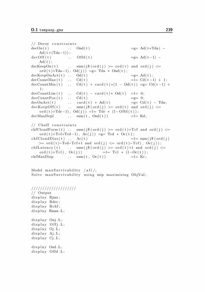
D.1 tempasp.gms 239
// Decoy c on s t r a i n t sdecOn( t ) . . Ond( t ) =g= Ad( t+Tda) −
Ad( t+(Tda−1)) ;decOff ( t ) . . Offd ( t ) =g= Ad( t−1) −
Ad( t ) ;decKeepOn( t ) . . sum( j$ ( ord ( j ) >= ord ( t ) and ord ( j ) <=
ord ( t )+Tda−1) , Od( j ) ) =g= Tda ∗ Ond( t ) ;decKeepOnAct( t ) . . Od( t ) =g= Ad( t ) ;decCountMax ( t ) . . Cd( t ) =l= Cd( t−1) + 1 ;decCountMin ( t ) . . Cd( t ) + card ( t ) ∗(1 − Od( t ) ) =g= Cd( t−1) +
1 ;decCountLim ( t ) . . Cd( t ) − card ( t ) ∗ Od( t ) =l= 0 ;decCountPos ( t ) . . Cd( t ) =g= 0 ;decOnAct( t ) . . card ( t ) ∗ Ad( t ) =g= Cd( t ) − Tda ;decKeepOff ( t ) . . sum( j$ ( ord ( j ) >= ord ( t ) and ord ( j ) <=
ord ( t )+Tdr−1) , Od( j ) ) =l= Tdr ∗ (1−Offd ( t ) ) ;decMaxDepl . . sum( t , Ond( t ) ) =l= Kd;
// Chaff c on s t r a i n t schfCloudForm ( t ) . . sum( j$ ( ord ( j ) >= ord ( t )+Tcf and ord ( j ) <=
ord ( t )+Tcf+Tcd−1) , Ac( j ) ) =g= Tcd ∗ Oc( t ) ;ch fCloudDiss ( t ) . . Ac( t ) =l= sum( j$ ( ord ( j )
>= ord ( t )−Tcd−Tcf+1 and ord ( j ) <= ord ( t )−Tcf ) , Oc( j ) ) ;chfLatency ( t ) . . sum( j$ ( ord ( j ) >= ord ( t )+1 and ord ( j ) <=
ord ( t )+Tcl ) , Oc( j ) ) =l= Tcl ∗ (1−Oc( t ) ) ;chfMaxDisp . . sum( t , Oc( t ) ) =l= Kc ;
Model maxSurv ivab i l i ty / a l l / ;Solve maxSurv ivab i l i ty us ing mip maximizing ObjVal ;
////////////////////// Outputd i sp l ay Rjmr ;d i sp l ay Rdec ;d i sp l ay Rchf ;d i sp l ay Rmax.L ;
d i sp l ay Onj .L ;d i sp l ay O f f j .L ;d i sp l ay Oj . L ;d i sp l ay Aj . L ;d i sp l ay Cj . L ;
d i sp l ay Ond .L ;d i sp l ay Offd .L ;

240 The GAMS Program
d i sp l ay Od.L ;d i sp l ay Ad .L ;
d i sp l ay Oc .L ;d i sp l ay Ac .L ;d i sp l ay a .L ;
d i sp l ay Ssum .L ;d i sp l ay objVal . L ;
F i l e out The r e s u l t s / tempasp . r e s / ;out . nd=5;out . ap=1;Put out ;Put system . date ,
@10 system . time ,@20 card ( t ) ,@30 Ssum .L ,@42 ObjVal . L ,@62 system . e lapsed ,@70 ’%gams . user1 % ’;
PutClose out ;
Appendix E
Software and Hardware
This appendix gives a short description of parts of the software and hardwareinvolved in the development of the models described in the work.
E.1 Software
This section describes the software that is used for main parts of the develop-ment. Where extra information is available on the Internet relevant URLs aregiven.
B-Prolog For the development and tests of the Prolog program described inChapter 4 the B-Prolog interpreter is used. This is chosen since it seemsrobust, it has an easy to use prompt interface, it is fairly well documented,and it is free for academic use.
B-Prolog can be downloaded from http://www.probp.com/.
HUGIN During development of the BN described in Chapter 5 version 6.3 ofHUGIN is used. The tests have been performed using HUGINTM version6.7 (build 6702).
242 Software and Hardware
A limited version of HUGIN, known as HUGIN LiteTM, can be downloadedfor free from http://www.hugin.com/. Following platforms are covered:Windows, Solaris Sparc, Solaris x86, Linux, Mac OS X 10.3, and Mac OSX 10.4.
Fly-In The Fly-In 2000 GUI version 2.3.4 software is used to produce data forthe Structural Learning of a BN. The software comes with the followingmessage: ”The Fly-In software was produced and released to EWS 5/SCI-067 by DSTL.”
MATLAB MATLAB is used for the construction of scenarios and the samplingof time steps used in both the mathematical model (Chapter 6) and withthe metaheuristics (Chapter 7). Various versions of MATLAB are used inthe work. For the final work MATLABr version 7.1.0.183, R14, ServicePack 3 is used.
See http://www.mathworks.com/ for more information on MATLAB.
GAMS In solving the mathematical model GAMS is run on a license given tothe Technical University of Denmark. The 140th revision, dated November11th, 2004, has been used.
Information on GAMS can be found at http://www.gams.com/.
CPLEX GAMS uses CPLEX as solver. The name ”CPLEX” comes from thecombination of the letter ”C” for the programming language, and theword ”simplex” for the simplex method for linear programming. Version9.130 of the ILOG CPLEX software is run. It is licensed to the TechnicalUniversity of Denmark.
http://www.ilog.com/gives more information on the ILOG CPLEX soft-ware.
E.2 Hardware
For most work a laptop PC with an Intel PentiumTM 4 1.79 GHz Mobile CPUand 512 MB of RAM is used. The PC is running Microsoft Windows XP, andit has been used to run B-Prolog, HUGIN, Fly-In, and MATLAB.
The mathematical model was developed and run on a SUN Fire 3800 1200 MHzwith 8 CPUs and 16 GB RAM running Solaris 9.
Implementing and running the metaheuristics is done using a stationary PCwith an AMD AthlonTM 64 X2 Dual Core Processor 4200+ 2.21 GHz and 2 GBof RAM. It is running Microsoft Windows XP.

E.2 Hardware 243
The dissertation is written using WinEdt/MikTeX running mainly on the laptopPC. Parts of the dissertation have been written on handheld devices such as aPalm III, a Compaq iPaq, and a Sony Ericsson K510i mobile phone.

244 Software and Hardware
Bibliography
[1] Directional infrared counter measures. [http://en.wikipedia.org/wiki/DIRCM],February 2007.
[2] ECLiPSe. [http://eclipse.crosscoreop.com/], March 2007.
[3] International Society for Bayesian Analysis. [http://www.bayesian.org/],March 2007.
[4] MIL-STD-1553. [http://en.wikipedia.org/wiki/MIL-STD-1553], March2007.
[5] OODA Loop. [http://en.wikipedia.org/wiki/OODA Loop], March 2007.
[6] The Missile Index. [http://missile.index.ne.jp/], February 2007.
[7] Stig K. Andersen, Kristian G. Olesen, Finn V. Jensen, and Frank Jensen.HUGIN – a shell for building Bayesian belief universes for expert systems.pages 332–337, 1990.
[8] Virginia Apgar. A proposal for a new method of evaluation of the newborninfant. Current Researches in Anesthesia and Analgesia, pages 261–262,July-August 1953.
[9] J.M. Arroyo and A.J. Conejo. Optimal response of a thermal unit to anelectricity spot market. IEEE Transactions on Power Systems, 15(3):1098–1104, 2000.
[10] Robert E. Ball. The Fundamentals of Aircraft Combat Survivability Anal-ysis and Design. AIAA Education Series. Naval Postgraduate School, 2edition, 2003.
246 BIBLIOGRAPHY
[11] Sheila B. Banks and Carl S. Lizza. Pilot’s associate: a cooperative,knowledge-based systemapplication. IEEE Expert, 6(3):18–29, June 1991.
[12] Ivan Bratko. PROLOG Programming for Artificial Intelligence. Addison-Wesley, 2. edition, 1990.
[13] Bruce D’Ambrosio. Inference in Bayesian networks. AI Magazine, 20(2):21–36, 1999.
[14] Danish Defence Research Establishment. Maaleradarsystemet mrs.
[15] Kathryn A. Dowsland. Modern heuristic techniques for combinatorial prob-lems, chapter 2, pages 20–69. John Wiley & Sons, Inc., New York, NY,USA, 1993.
[16] Morten Enevoldsen. Decision support for fighter pilots. Master’s thesis,Informatics and Mathematical Modelling, Technical University of Denmark,DTU, Richard Petersens Plads, Building 321, DK-2800 Kgs. Lyngby, 2003.
[17] Peter Haddawy. An overview of some recent developments in Bayesianproblem solving techniques. AI Magazine, Summer 1999.
[18] Jonas Lundbek Hansen, Steen Søndergaard, and Erik Thisen. FOFT EKtaktiske træner. FOFT Nyt, (3), December 2003.
[19] Hovland Harald. Optimisation of flare and chaff programs – an analyti-cal approach. Technical Report 2006/01460, Norwegian Defence ResearchEstablishment, 2006.
[20] Clyde W. Holsapple and Andrew B. Whinston. Decision Support Systems– A Knowledge-Based Approach. West Publishing Company, 1996.
[21] Finn Verner Jensen. An introduction to Bayesian networks. UCL Press,1996.
[22] Finn Verner Jensen. Bayesian Networks and Decision Graphs. SpringerVerlag, 2001.
[23] Uffe Bro Kjærulff and Anders L. Madsen. Probabilistic Networks – AnIntroduction to Bayesian Networks and Influence Diagrams. Aalborg Uni-versity, 2005.
[24] E. C. Labatt, Jr., editor. Automated threat response recommendation in en-vironments of high data uncertainty using the Countermeasure AssociationTechnique (CMAT), September 1991.
[25] Helge Langseth and Thomas D. Nielsen. Fusion of domain knowledge withdata for structural learning in object oriented domains. Journal of MachineLearning Research, 4, 2003.
BIBLIOGRAPHY 247
[26] Steffen L. Lauritzen. The EM algorithm for graphical association modelswith missing data. Comput. Stat. Data Anal., 19(2):191–201, 1995.
[27] H.R. Lourenco, O. Martin, and T. Stutzle. A beginner’s introduction toiterated local search. In Proceedings of the Fourth Metaheuristics Interna-tional Conference, volume 1, pages 1–6, 2001.
[28] Anders L. Madsen, Michael Lang, Uffe B. Kjærulff, and Frank Jensen. TheHugin tool for learning Bayesian networks. In Lecture Notes in ComputerScience, volume 2711, April 2004.
[29] Bruce A. McCarl. GAMS User Guide. Texas A&M University, 22.2 edition,March 2006. Developed in cooperation with GAMS Development Corpo-ration.
[30] Jamison Jo Medby and Russell W. Glenn. Street Smart: Intelligence Prepa-ration of the Battlefield for Urban Operations. 2002.
[31] F. W. Moore. A methodology for missile countermeasures optimizationunder uncertainty. Evolutionary Computation, 10(2):129–149, 2002.
[32] F. W. Moore and O. N. Garcia. A genetic programming methodology formissile countermeasures optimization under uncertainty. Lecture Notes inComputer Science, (1447):367–376, 1998.
[33] John H. Painter, III Wallace E. Kelly, Jeffrey A Tang, Kristopher A. Lee,Paul A. Branham, John W. Crump, Donald T. Ward, Karthik Krishna-murty, Disk L. Y. Woo, William P. Alcorn, Andrew C. Robbins, and Ren-Jye Yu. Decision support for the general aviation pilot. In Proceedings of the1997 IEEE International Conference on Systems, Man, and Cybernetics,Orlando, FL, October 1997.
[34] Judea Pearl. Probabilistic Reasoning in Intelligent Systems: Networks ofPlausible Inference. Morgan Kaufmann, 1988.
[35] William H. Press, Saul A. Teukolsky, William T. Vetterling, and Brian P.Flannery. Numerical recipes in FORTRAN: the art of scientific computing.Cambridge University Press, New York, NY, USA, 2. edition, 1992.
[36] A. Quan, R. Crawford, H. Shao, K. Knudtzon, A. Schuler, D. Scott, S Hay-ati, Jr Higginbotham, R., and R. Abbott. Automated threat response usingintelligent agents (ATRIA). Aerospace Conference, 2001, IEEE Proceed-ings, 6:2721–2730, March 2001.
[37] Per Husmann Rasmussen. Feasibility-studie, Intelligente Systemer, chapter4, ,,Beslutningsstøttesystem”, pages 15–19. Royal Danish Defence College,March 2003.
248 BIBLIOGRAPHY
[38] Mathias Ravn and Lars Vadstrup Hansen. Neuroevolution af computer-styrede pokerspillere uden anvendelse af ekspertstrategi. Master’s thesis,University of Aarhus, November 2005.
[39] William B. Rouse, Normann D. Geddes, and John M. Hammer. Computer-aided fighter pilots. IEEE Spectrum, 27(3):38–41, March 1990.
[40] Sadiq M. Sait and Habib Youssef. Iterative Computer Algorithms with Ap-plications in Engineering: Solving Combinatorial Optimization Problems.IEEE Computer Society Press, Los Alamitos, CA, USA, 1999.
[41] D. Curtis Schleher. Introduction to Electronic Warfare. Artech House,1986.
[42] M.I. Skolnik. Radar Handbook. McGraw-Hill, 1970.
[43] Steen Søndergaard. FOFT støtter flyvevabnet ved NATO forsøg. FOFTNyt, (2), August 1998.
[44] P. Spirtes, C. Glymour, and R. Schneies. Causation, Prediction, andSearch. Adaptive Computation and Machine Learning. MIT Press, 2 edi-tion, January 2000.
[45] Peter Spirtes and Clark Glymour. An algorithm for fast recovery of sparsecausal graphs. Social Science Computer Review, 9(1), 1991.
[46] G.W. Stimson. Introduction to Airborne Radar. SciTech Publishing, Inc.,2. edition, 1998.
[47] Dan Stromberg. Decision-making using temporal reasoning. IJCAI’99Workshop on Teams, 1999.
[48] Peter Svenmarck. Decision support in a fighter aircraft: From expert sys-tems to cognitive modelling. HFA Report 1998-04, Linkopings Universitet,Swedish Centre for Human Factors in Aviation, 1998.
[49] Peter Svenmarck and Sidney Dekker. Decision support in fighter aircraft:From expert systems to cognitive modelling. Behaviour and InformationTechnology, 22(3):175–184, 2003.
[50] G. Teasdale and B. Jennett. LANCET (ii), pages 81–83, 1974.
[51] Terma. AN/ALQ-213(V) Electronic Warfare Management System.Brochure.
[52] Jim D. Titley. Integrated Defensive Aids Systems, a matter of definition.DDRE Report F-13/2003, Danish Defence Research Establishment, 2003.
BIBLIOGRAPHY 249
[53] Thomas Verma and Judea Pearl. An algorithm for deciding if a set ofobserved independencies has a causal explanation. In Proceedings of theeighth conference on Uncertainty in Artificial Intelligence, pages 323–330,San Francisco, CA, USA, 1992. Morgan Kaufmann Publishers Inc.
[54] Patrick Henry Winston. Artificial Intelligence. Series in Computer Science.Addison-Wesley, 2. edition, 1984.
[55] Fred Wright. Automated electronic warfare with threat response process-ing. Georgia Tech Research Institute, May 2006.
[56] Neng-Fa Zhou. B-Prolog User’s Manual. Afany Software, December 2006.
Related Documents


