DECISION SUPPORT FOR URBAN WIND ENERGY EXTRACTION

Welcome message from author
This document is posted to help you gain knowledge. Please leave a comment to let me know what you think about it! Share it to your friends and learn new things together.
Transcript

DECISION SUPPORT FOR URBAN WIND ENERGY EXTRACTION

DECISION SUPPORT FOR
URBAN WIND ENERGY EXTRACTION
By
RUTH C. COOPER, B.ENG
A Thesis
Submitted to the School of Graduate Studies
in Partial Fulfilment of the Requirements
for the Degree
Master of Applied Science (M.A.Sc.)
McMaster University

Department of Civil Engineering
© Copyright by Ruth C. Cooper, July 2007
ii

MASTER OF APPLIED SCIENCE (2007) McMaster
University
(Civil Engineering) Hamilton, Ontario
TITLE: Decision Support for Urban Wind Energy Extraction
AUTHOR: Ruth C. Cooper, B.Eng. (Carleton University)
SUPERVISOR: Dr. Brian W. Baetz
NUMBER OF PAGES: xxii, 247
ii

ABSTRACT
In the wake of the environmental movement theburgeoning wind energy industry, equipped with arudimentary understanding of the wind resource andlimited socio-economic policies, created today's windenergy paradigm characterised by farms of tower-mounted, 3-bladed, horizontal-axis wind turbines(HAWTs). This research undertaking proposes that aparadigm shift is in order and that commissioning ofdecentralised, in-situ, urban-scale wind energyconversion devices could assist the industry.
Project WEB, which was commissioned by the EuropeanUnion in the framework of Joule III (2000) to explorethe aerodynamic properties of built structures andsuitable wind energy conversion system configurations,coined the terms Urban Wind Energy Conversion System(UWECS) and Building Augmented Wind Turbine (BAWT).The theory behind BAWTs is primarily founded on largeskyscrapers and building-integrated HAWTs. Thisresearch undertaking focused on alternativelyconfigured UWECS and the potential of smaller buildings(e.g., residential and commercial buildings) to producesufficient building aerodynamics-induced windamplification to make urban wind energy generation aviable option.
The assessment of urban morphology-induced windamplification, specifically in support of sitingbuilding-integrated and/or mounted UWECSs, is a veryrecent undertaking. Only a small number of windturbine manufacturers are even exploring thedevelopment of suitably-scaled devices whoseperformance characteristics are tailored to urban windconditions. As such, this research explored thefeasibility of BAWT-theory in an urban setting through
iii

the development of a prototype Urban Wind EnergyPlanning (UWEP) Decision Support System (DSS).
The prototype UWEP DSS focuses primarily onbuilding aerodynamics-induced wind amplification,including consideration of peak-wind seasons.Microsoft® Excel was selected as the platform for theUWEP DSS, supporting development of user forms andintegral databases. This tool is intended for a broadrange of users, including the average home owner, UWECSdevelopers, and energy planners. With minimal userinput, the UWEP DSS determines the mean wind speedwithin the amplification zones, the location of theamplification zones, and the energy that couldpotentially be generated by an appropriately-sitedUWECS.
Two case study applications of the UWEP DSS wereconducted to validate the estimations and demonstratethe capabilities of the tool. The University ofToronto Robarts Library application and the GreenVenture EcoHouse application yielded credible mean windspeed and potential wind energy estimates on comparisonto the online wind atlases. The EcoHouse case studyapplication included the selection and siting ofvarious UWECSs. It highlighted the potential of ahypothetical wind energy conversion device being ableto generate almost 40% of the 700 kWh per month,average household energy demand. Conversely, itdemonstrated that the traditional tower-mountedhorizontal axis wind turbines, situated outside of thepotential amplification zones in accordance withcurrent siting guidelines, would only be able togenerate 5% of the demand.
By demonstrating the prototype UWEP DSS through aninstitutional and a residential application case study,it is hoped that the scope and capabilities of, and the
iv

amplified wind energy potential identified by, thistool will foster further research in urban wind energyplanning, building aerodynamics-induced amplificationassessment, and development of new UWECSs. Theprototype UWEP DSS appears to be the first to estimatebuilding aerodynamics-induced amplification from peakcomposite pressure-gust coefficients published inbuilding codes. Further research is recommended togain a better understanding of sustained, as opposed topeak, wind amplification. The modular nature of theUWEP DSS lends itself to the modifications that willundoubtedly be required as further knowledge isdeveloped in this field.
v

ACKNOWLEDGEMENTS
As I reflect on the last twenty months, I can nothelp but to feel a pang of regret to see this stage ofmy life come to an end. I will surely miss the highsand lows that accompany the thrill of discovery and thedespair in failed hypotheses. I would like to takethis opportunity to acknowledge a few key individualswho supported me through times during which thechallenges appeared insurmountable.
First and foremost, I appreciate having beenprovided with this opportunity to expound on thevirtues of Dr. Brian Baetz. I initially contacted Dr.Baetz out of interest in pursuing graduate studieswithin the department of Civil Engineering at McMasterin the spring of 2005. Without his support andassistance throughout the whole application process, Iwould not have been afforded the opportunity to conductresearch as a Masters candidate. Especially during thelast few months, his continued support, encouragement,and ability to sort the wheat from the chaff, so tospeak, have been invaluable. I would also like tothank Drs. Sarah Dickson and Michael Tait of theDepartment of Civil Engineering for their contributionsas thesis examination committee members.
The association with the Barry Rawn's team at theUniversity of Toronto was a fortuitous accident,instigated by Dr. Ursula Franklin. The data providedby this team of urban wind energy enthusiasts are whathelp to ground the results produced by application ofthe UWEP DSS in reality.
The concept of building aerodynamics induced windamplification, which started as a mere notion, wouldnot have been substantiated had it not been for theresearch conducted by Mr. Neil Campbell and associates
vi

under the auspices of Project WEB. Further research onBAWT theory conducted at TU Delft by Dr. Gerard vanBussel and Dr. Sander Mertens yielded numerous journalarticles, the collection of which I refer to as 'thebible'.
Assessment of the mean wind speed below the urbancanopy layer would not have been possible were it notfor the work of Dr. Robert MacDonald of the Universityof Waterloo. Unfortunately, in attempting to contacthim, I discovered that he had passed away in April of2004.
Last, but by no means least, this researchundertaking would not have been possible without thesupport of the staff and faculty of the Department ofCivil Engineering.
vii

TABLE OF CONTENTS
ABSTRACT....................................iii
ACKNOWLEDGEMENTS..............................v
LIST OF FIGURES...............................x
LIST OF TABLES.............................xiii
NOMENCLATURE................................xiv
1 INTRODUCTION...............................11.1 Climate Change and Government / Industry Response..........................................31.2 The Wind Energy Industry......................71.3 The Building Industry........................111.4 Building Aerodynamics........................141.5 Urban Wind Energy Conversion Systems.........161.6 Scope and Objectives of the Research Undertaking......................................191.7 Thesis Structure.............................21
2 LITERATURE REVIEW.........................222.1 The Interdisciplinary Nature of this Research 232.2 Wind Power Meteorology Overview..............252.3 The Urban Boundary Layer.....................27
2.3.1..........................The Wind Climate31
2.3.2...................Frequency Distributions34
2.4 Boundary Layer Modelling.....................362.4.1..........................Mesoscale Models
372.4.2.........................Microscale Models
38
viii

2.4.3........................Model Combinations39
2.5 The Wind Atlas...............................412.5.1............The Canadian Wind Energy Atlas
472.5.2...........The Ontario Wind Resource Atlas
492.6 Wind Atlas Methodology.......................52
2.6.1...............The Mean Wind Speed Profile54
2.7 Wind Resource Assessment.....................562.7.1.......................Commercial Software
592.8 The Built Environment........................62
2.8.1........................Urban Canopy Layer62
2.8.2............Urban Parameterisation Schemes64
2.8.3...................Mean Wind Speed Profile65
2.8.4.....................Building Aerodynamics67
2.9 Decision Support Systems.....................762.10......................Literature Review Summary
81
3 CONCEPTUAL MODEL DEVELOPMENT..............833.1 Urban Renewable Energy Source Assessment.....843.2 Scope of Applicability.......................863.3 Configuration of the Conceptual Model........873.4 Wind Energy Assessment Methodology...........90
3.4.1.............Meteorological Considerations90
3.4.2..............Morphological Considerations92
4 DECISION SUPPORT SYSTEM DEVELOPMENT.......96
ix

4.1 Overview.....................................984.2 User Interface..............................1014.3 External Databases..........................1034.4 Internal Database...........................104
4.4.1............Roughness Classification Table105
4.4.2..............Urban Parameterisation Table108
4.4.3...........Wind Amplification Factor Table113
4.5 UWEP module.................................1184.5.1....................Wind Data Extrapolator
1214.5.2....................Wind Data Interpolator
1314.5.3............................Wind Amplifier
1344.5.4.........................Energy Calculator
1464.6 Summary Report..............................1484.7 Architectural Configurator..................148
5 APPLICATION OF THE DECISION SUPPORT SYSTEM1505.1 Institutional Case Study....................151
5.1.1.............Annual Wind Energy Assessment1525.1.1.1..................Mean Wind Climate
1535.1.1.2..........Amplified Mean Wind Speed
1605.1.1.3........................Wind Energy
1705.1.1.4.....................Summary Report
1725.1.2...........Seasonal Wind Energy Assessment
173
x

5.1.2.1..................Mean Wind Climate174
5.1.2.2..........Amplified Mean Wind Speed179
5.1.2.3........................Wind Energy181
5.1.3........UWEP DSS Credibility Investigation1825.1.3.1..................Mean Wind Climate
1845.1.3.2.................Wind Power Density
1935.1.3.3........................Limitations
1955.2 Residential Case Study......................196
5.2.1..............Mean Annual Energy Potential198
5.2.2.............UWECS Selection and Placement201
5.2.3.............Architectural Reconfiguration209
5.2.4. .Potential Limitations of the Application210
6 SUMMARY, CONCLUSIONS & RECOMMENDATIONS...2136.1 Summary.....................................2136.2 Conclusions.................................2156.3 Recommendations.............................220
7 REFERENCES...............................228
xi

APPENDICES
Appendix A Boundary Layer Meteorology PrimerAppendix B Wind Atlas Comparison TableAppendix C Topographical Acceleration PrimerAppendix D - 1 Development of the Roughness Classification TableAppendix D - 1a Roughness Classification SchemesAppendix D - 2 Development of the Urban Parameterisation TableAppendix D - 3 Development of the Wind Amplification Factor TableAppendix E Background and Assumptions: Wind Data ExtrapolationAppendix F Background and Assumptions: Wind Data InterpolationAppendix G Background and Assumptions: Wind AmplificationAppendix H Background and Assumptions: Energy CalculationAppendix I - 1 Wind Statistics WorksheetAppendix I - 2 Wind Amplification WorksheetAppendix I - 3 Wind Energy WorksheetAppendix I - 4a Equation SummaryAppendix I - 4b Internal Database Development WorkbookAppendix J - 1a Robarts Library: Summary ReportAppendix J - 1b Robarts Library: Wake Streamline PlotsAppendix J - 2a Green Venture EcoHouse: Summary ReportAppendix J - 2b Green Venture EcoHouse: Wake StreamlinePlotsAppendix K UWECS Photo MontageAppendix L Economic Assessment Tools matrixAppendix M Anemometer Heights of Canadian Meteorological StationsAppendix N UWEP DSS Application
xii

LIST OF FIGURES
Figure 1.1. Brush Windmill Cleveland, OH (1888).. . . .1Figure 1.2. Wind Farm in Coachella Valley, California
(US)..............................................2Figure 1.3. G8 Countries CO2 emissions per capita for
1990 and 2002.....................................3Figure 1.4. Canadian stationary source combustion GHG
Emissions (2004)..................................4Figure 1.5. Canadian electricity generation source mix
in GW (2004)......................................6Figure 1.6. Ontario electricity generation source mix
in GW (2007)......................................7Figure 1.7. Installed wind energy capacity (GW) by
country as of 12/2006.............................8Figure 1.8. Technical renewable energy potential in
Canada in GW by source............................8Figure 1.9. Building Augmented Wind Turbines.......10Figure 1.10. An artists rendition of the Burj al-Taqa
(Energy Tower)...................................12Figure 1.11. General WECS Configurations...........16Figure 1.12. Rooftop wind energy conversion devices.
.................................................17Figure 1.13. Modular Rooftop modular wind energy
conversion devices...............................17Figure 1.14. Building augmented wind energy conversion
systems..........................................18Figure 2.1. The interdisciplinary blocks of urban wind
energy research..................................24Figure 2.2. The Osaka City 'klimatope'.............26Figure 2.3. Urban boundary layer structural sketch. 28Figure 2.4. The terrain dependent velocity shear
profiles.........................................29Figure 2.5. Variation of the primary northern
hemisphere wind climates.........................32Figure 2.6. The components of the instantaneous wind
speed............................................33
xiii

Figure 2.7. Northern hemisphere wind climate frequencydistributions....................................34
Figure 2.8. The Toronto Island airport wind directionrose of June 2005................................35
Figure 2.9. Flow chart of the Riso wind power prediction model.................................40
Figure 2.10. Wind Energy Resource Atlas of the United States...........................................42
Figure 2.11. Analyzed Winter Season Average Wind Resource Maps....................................43
Figure 2.12. Wind resource estimates in the Northwest region of the US.................................44
Figure 2.13. The wind resource in Europe at 50 m a.g.l..................................................46
Figure 2.14. Worldwide status of the wind atlas methodology......................................47
Figure 2.15. The 65 tiles or quadrangles of the Canadian Wind Energy Atlas.......................48
Figure 2.16. Canadian Wind Atlas Quadrangle 40 - Mean Wind Speed at 30m................................49
Figure 2.17. Ontario Wind Resource Atlas demonstration....................................51
Figure 2.18. Wind Atlas Methodology flow chart.. . . .52Figure 2.19. Wind atlas methodology removal &
application of local effects.....................53Figure 2.20. PBL Day and night mean wind speed
profiles.........................................54Figure 2.21. Sketch of mean wind speed profile.. . . .55Figure 2.22. General form of packaged wind resource
assessment software..............................58Figure 2.23. Digital still video aerial imagery
extraction techniques............................65Figure 2.24. Flow regimes within the UCL...........69Figure 2.25. Vortex structure categorisation.......71Figure 2.26. Effect of varying building height on
canyon vortex structure..........................72
xiv

Figure 2.27. Effect of roof configuration on canyon vortex structure.................................73
Figure 2.28. Cross-canyon horizontal mean wind speed variation........................................74
Figure 2.29. The flow chart of the DAD-based WiLDE application......................................77
Figure 2.30. Solar energy decision support system.. 80Figure 3.1. Urban Renewable Energy Source (URES) DSS.
.................................................84Figure 3.2. Conceptual Model of the UWEP DSS.......87Figure 3.3. The vertical stratification of the urban
boundary layer...................................91Figure 3.4. Wind speed histogram (a) and direction
rose (b).........................................92Figure 3.5. Morphology-induced wind amplification.. 94Figure 4.1. Block model of the UWEP DSS............97Figure 4.2. Illustrative representation of the UWEP
module’s methodology............................100Figure 4.3. The Control Centre of the UWEP DSS.. . .102Figure 4.4. The logarithmic wind speed profile.. . .106Figure 4.5. The sky view factor as a measure of street
canyon geometry.................................109Figure 4.6. The geometry of urban morphology.......111Figure 4.7. Satellite plan image of urban subregion
category # 1....................................112Figure 4.8. Cubic array representation of urban
subregion category # 1..........................112Figure 4.9 Neighbourhood-scale aerodynamic effects.
................................................115Figure 4.10. Idealised representations of building-
scale aerodynamic effects.......................116Figure 4.11. Idealised 3D representation of the UBL
sublayers.......................................120Figure 4.12. The WDE submodule of the UWEP module. 122Figure 4.13. The Project Details tab of the Site
Specification form..............................123
xv

Figure 4.14. The Location tab of the Site Specification form..............................124
Figure 4.15. The Topographical tab of the Site Specification form..............................125
Figure 4.16. The Meteorological tab of the Site Specification form (annual).....................126
Figure 4.17. The Meteorological tab of the Site Specification form (seasonal)...................127
Figure 4.18. The mean wind speed profile generated by the WDI.........................................133
Figure 4.19. The Wind Amplifier submodule of the UWEP module..........................................135
Figure 4.20. The Neighbourhood Morphology form.. . .136Figure 4.21. The relationship of urban road type
classifications.................................137Figure 4.22. Typical cross-sectional elements of an
urban road......................................138Figure 4.23. Reconfigured cubic array of category # 1.
................................................138Figure 4.24. The critical angles..................139Figure 4.25. The Aerodynamic Effects form.........140Figure 4.26. The Building Features form...........142Figure 4.27. Linear and angular building-specific
variables.......................................143Figure 4.28. Plan (left) and elevation (right) wake
zone developments...............................144Figure 4.29. Amplification zones..................145Figure 4.30. The Architectural Configurator module of
the UWEP DSS....................................148Figure 5.1. Robarts Library (left) and the Green
Venture EcoHouse (right)........................151Figure 5.2. The southeast side of the J.P. Robarts
Library.........................................152Figure 5.3. The John P. Robarts Research Library.. 153Figure 5.4. A satellite image of a portion of the St.
George campus...................................154
xvi
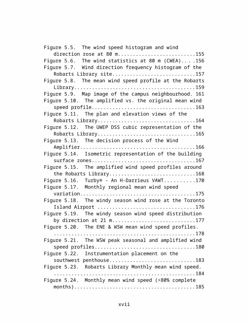
Figure 5.5. The wind speed histogram and wind direction rose at 80 m..........................155
Figure 5.6. The wind statistics at 80 m (CWEA).. . .156Figure 5.7. Wind direction frequency histogram of the
Robarts Library site............................157Figure 5.8. The mean wind speed profile at the Robarts
Library.........................................159Figure 5.9. Map image of the campus neighbourhood. 161Figure 5.10. The amplified vs. the original mean wind
speed profile...................................163Figure 5.11. The plan and elevation views of the
Robarts Library.................................164Figure 5.12. The UWEP DSS cubic representation of the
Robarts Library.................................165Figure 5.13. The decision process of the Wind
Amplifier.......................................166Figure 5.14. Isometric representation of the building
surface zones...................................167Figure 5.15. The amplified wind speed profiles around
the Robarts Library.............................168Figure 5.16. Turby® - An H-Darrieus VAWT..........170Figure 5.17. Monthly regional mean wind speed
variation.......................................175Figure 5.18. The windy season wind rose at the Toronto
Island Airport .................................176Figure 5.19. The windy season wind speed distribution
by direction at 21 m............................177Figure 5.20. The ENE & WSW mean wind speed profiles.
................................................178Figure 5.21. The WSW peak seasonal and amplified wind
speed profiles..................................180Figure 5.22. Instrumentation placement on the
southwest penthouse.............................183Figure 5.23. Robarts Library Monthly mean wind speed.
................................................184Figure 5.24. Monthly mean wind speed (>80% complete
months).........................................185
xvii

Figure 5.25. The windy season wind rose vs. TIA data veered 90 degrees...............................186
Figure 5.26. Wind direction frequency comparison.. 187Figure 5.27. The windy season wind speed distribution
comparison......................................188Figure 5.28. The primary & secondary direction wind
speed distributions.............................189Figure 5.29. Computational fluid dynamics models
created by CFX..................................190Figure 5.30. Wind power density at 80 m (CWEA) with
Toronto inset...................................194Figure 5.31. Idealised representation of conical
delta-wing vortices.............................195Figure 5.32. The extensions of the Robarts Library.
................................................196Figure 5.33. The Green Venture EcoHouse - Then & Now.
................................................197Figure 5.34. The UWEP DSS representation of the
EcoHouse........................................198Figure 5.35. EcoHouse site wind direction rose
overlay.........................................200Figure 5.36. Power coefficient as a function of tip
speed...........................................202Figure 5.37. UWECSs proposed for installation at the
EcoHouse site...................................204Figure 5.38. Roof ridge and ground mounted UWECSs at
the EcoHouse Site...............................207Figure 6.1. The Bahrain World Trade Center........217Figure 6.2. Primary and secondary wind speed frequency
distributions (TIA).............................222Figure 6.3. Velocity in a Rankine Vortex..........225Figure 6.4. Sun and wind orientation diagram......226
xviii

LIST OF TABLES
Table 2.1. Causes and time scale of temporal wind variation........................................31
Table 2.2. Broad-scale classification of meteorological models............................36
Table 2.3. Wind Resource Estimation Methods.........57Table 2.4. Commercial Wind Resource Assessment
Software.........................................60Table 4.1. The Roughness Classification table of the
UWEP DSS........................................105Table 4.2. The urban subregions of the Urban
Parameterisation table..........................110Table 4.3. Neighbourhood-scale Wind Amplification
Factor table....................................114Table 4.4. Pressure coefficient-based Wind
Amplification Factor table......................117Table 5.1. The wind direction frequencies for the
Robarts Library site............................156Table 5.2. Wind Statistics Summary................158Table 5.3. Representative neighbourhood street
characteristics.................................161Table 5.4. Neighbourhood inter-building spaces and
angles of flow incidence........................162Table 5.5. Summary of the first stage of the
amplification assessment........................162Table 5.6. Summary of the second stage of the
amplification assessment........................167Table 5.7. Characteristic dimensions and amplification
zone areas......................................169Table 5.8. Wind power by building face and zone at the
Robarts Library.................................171Table 5.9. Mean annual wind energy by building face
and zone........................................172Table 5.10. Summary of the WSW amplification
assessment......................................179
xix

Table 5.11. The peak season contributions from the WSWwind direction..................................181
Table 5.12. Mean wind speed and direction summaries.................................................191
Table 5.13. Mean wind speed and associated wind power density comparison..............................193
Table 5.14. Wind energy by building face and zone at the EcoHouse....................................198
Table 5.15. EcoHouse building face-specific assessmentsummary.........................................199
Table 5.16. Performance characteristics of the proposed UWECSs.................................205
Table 5.17. UWECS power generation and percent of rated power.....................................209
Table 5.18. Roof top wind energy by building face at the EcoHouse....................................210
xx

NOMENCLATURE
Nomenclature Primer
Due to conflicting symbol-definitions both within theboundary layer meteorology literature and between thevarious disciplines, some compromises had to be made.For example, h appears as the height of the boundarylayer and the reference height on a building, urepresents the wind speed and the horizontal componentthereof, and P is used to designate both power andpressure.For most cases these conflicts were left unresolvedsince the multiple definitions did not come to bearwithin the same context. For example, B is usedthroughout to designate building breadth, a geostrophicdrag law constant, and a transitional profile equationparameter. In situations where there appeared to be anindustry standard more specifically applicable to thisundertaking, it was adopted for the body of the textand equated to the variables ascribed to the graphs ortables from the literature presented in the section.For example, the designation of building width as Bused within the building code was adopted as opposed tousing B to represent the street canyon width, as isdone in the wind power meteorology literature. Thistype of inconsistency is locally defined as anexception. In other cases, new symbols were introduced(e.g., M for wind magnitude).In general, subscripts are used to maintain consistencyand convention (e.g., D typically designates buildingdepth, so DS is used to designate the smaller of thetwo building plan dimensions (i.e., B & D)). Whenessentially identical variables already adorned withsubscripts occur within the same section, lower andupper case subscripts are used (i.e., CP (pressurecoefficient) vs. Cp (coefficient of performance)).
xxi

Nomenclature is presented in two sections: Acronyms andNotation. Subscripted variables not listed in theNotation section are defined in the Subscripts sub-section of the Notation section.
Acronyms
ABL Atmospheric Boundary Layeragl above ground levelART Advanced Renewable TariffsASCE American Society of Civil Engineersasl above sea levelBAWT Building Augmented Wind TurbineBEPA Biomass Energy Potential AssessmentBLWT Boundary Layer Wind TunnelBRE Building Research EstablishmentBREDEM Building Research Establishment Domestic
Energy ModelBREEAM Building Research Establishment Environmental
Assessment MethodBUWT Building augmented, integrated, and/or
mounted Wind TurbineCanWEA Canadian Wind Energy AssociationCERI Canadian Energy Research InstituteCETC CANMET Energy Technology CentreCFD Computational Fluid DynamicsCHC Canadian Hydraulics Centre (NRC)COM COMpressed (referring to climate data sets)CORINE CoORdination of INformation on the
EnvironmentCPZ Control Potential ZonesCT Canadian TireCWE Computational Wind EngineeringCWEA Canadian Wind Energy AtlasDAD Database-Assisted DesignDD Decimal-DegreesDEM Digital Elevation Model or MapDM Degrees:Minutes
xxii

DMS Degrees:Minutes:SecondsDOE Department of Energy (US)DSM Digital Surface ModelDSS Decision Support SystemDTM Digital Terrain MapEC Environment CanadaECMRF European Centre for Medium Range (weather)
ForecastingEEP Energy and Environmental PredictionEnSim Environmental SimulationEP Energy PlanningeQuest QUick Energy Simulation ToolEU European UnionEWEA European Wind Energy Associationfad frontal area density [f]far frontal aspect ratio [B or L / H]FIWF Fully Independent Wake FlowFRG Federal Republic of GermanyFS Frontal Stagnation (point).fst Format Standard file format, formerly .rpnGEM Global Environmental MultiscaleGESIMA GEesthacht SImulation Model of the AtmosphereGFS Global Forecast SystemGHG Green House GasGIS Geographic Information SystemGPS Global Positioning SystemGS Ground Separation (point)GUI Graphical User InterfaceGWEC Global Wind Energy CouncilHAWT Horizontal Axis Wind TurbineHIRLAM HIgh Resolution Limited Area ModelHOMER Hybrid Optimization Model for Electric
RenewablesHPDM Hybrid Plume Dispersion ModelIBC International Building CodeIBL Internal Boundary LayerICC International Code Council
xxiii

IRF Isolated Roughness FlowISL Inertial Sub-LayerIWA Industrial Wind Action (Group)KAMM Karlsruhe Atmospheric Mesoscale ModelLEED Leadership in Energy and Environmental DesignLES Large Eddy SimulationLIDAR LIight Direction And RangingLSR Least-Squares RegressionLULUCF Land Use, Land Use-Change, and ForestryM Moments (Method of)MASS Mesoscale Atmospheric Simulation SystemMC2 Mesoscale Compressible CommunityML Maximum Likelihood (Method)MM5 Mesoscale Model - 5th generationMML Modified Maximum Likelihood (Method)mn monthMNR Ministry of Natural ResourcesMO Monin-ObukhovMODIS MODerate resolution Imaging SpectroradiometerMOS Model Output StatisticsMOST Monin-Obukhov Similarity TheoryMPAC Municipal Property Assessment CorporationMPC Measure-Predict-CorrelateMRF Medium Range Forecast (MRF)MSC Meteorological Service of CanadaMSFD Mixed Spectral Finite DifferenceNBC National Building CodeNCAR National Center for Atmospheric ResearchNCD&IA National Climate Data and Information ArchiveNCEP National Centers for Environmental PredictionNIMBY Not In My BackYardNOAA National Oceanic and Atmospheric
AdministrationNRCan Natural Resources CanadaNTS National Topographic SystemNWA Numerical Wind AnalysisNWP Numerical Weather Prediction
xxiv

OWA Observational Wind AnalysisOWRA Ontario Wind Resource Atlaspad plan area density [P]PBL Planetary Boundary LayerPCA Principle Component Analysispdf probability density functionPEI Prince Edward IslandPLEA Passive and Low Energy ArchitecturePNL Pacific Northwest LaboratoryPSS Planning Support SystemRANS Reynolds Averaged Navier-StokesRE Renewable EnergyRES Renewable Energy SourceRET Renewable Energy TariffsRETScreen Renewable Energy Technology ScreenRL Robarts Libraryrpm rotations per minuteRPN Recherche en Prévision NumériqueRSL Roughness SublayerRSME Root-Square Mean ErrorRST Retail Sales TaxRWC Regional Wind Climatesar side aspect ratio [D/H] or [W/H]SATP Standard Atmospheric Temperature & Pressure
(25 ºC & 101 kPa) ~ 1.169 kPa
SDSS Spatial Decision Support SystemSEP Solar Energy PlanningSF Skimming FlowSGS SubGrid Scale (LES CFD model based on
filtering)SISL Semi-Implicit Semi-LagrangianSOC Standard Offer Contract (also SOP)SOP Standard Offer ProgramSL Surface LayerSOI Spatial Openness IndexSP Separation Point
xxv

SRTM Shuttle Radar Topographic MissionSTP Standard Temperature & Pressure (0 ºC &
101.325 kPa)~ 1.293 kg/m3
SVF Sky View FactorTAC Transport Association of CanadaTI Turbulence IntensityTIA Toronto Island AirportTKE Turbulence Kinetic EnergyTMY Test Meteorological YearTRY Test Reference YearTSD Time Series DataTVM Temperature Variance MethodUBL Urban Boundary LayerUCL Urban Canopy LayerUHI Urban Heat IslandUQAM Université du Québec à MontréalURES Urban Renewable Energy SourceUS Unites States of AmericaUSGBC US Green Building CouncilUWECS Urban Wind Energy Conversion SystemUWEP Urban Wind Energy PlanningVAWT Vertical Axis Wind TurbineVBA Visual Basic for ApplicationsWAM Wind Atlas MethodologyWAsP Wind Atlas analysis and application ProgramWDE Wind Data ExtrapolatorWDI Wind Data InterpolatorWEB Wind Energy for the Built environmentWECS Wind Energy Conversion SystemWEP Wind Energy PlanningWEST Wind Energy Simulation ToolkitWFLC Wind Farm Location CriteriaWIF Wake Interference FlowWMO World Meteorological OrganisationWPD Wind Power Density W/m2
WWEA Worldwide Wind Energy Association
xxvi

ZED Zero Emissions Development
Notation
A geostrophic drag law constantA cross-sectional area (m2)A intermediate mean wind speed profile equation
parameterAd lot area (m2)Af frontal area (m2)Ap plan area (m2)AS swept area or characteristic area of a wind
energy conversion device (m2)At total area (m2)AZ amplification zone area (m2)a roughness layer height parameter, 2 < a < 5a attenuation coefficientB cross-wind building breadth (m)B geostrophic drag law constantB street canyon width, more typically
represented by W (m)B intermediate mean wind speed profile equation
parameterB/H frontal aspect ratio (far)b Rayleigh pdf parameterCD drag coefficientCg gust coefficientCP pressure coefficientCP Cg peak composite pressure-gust coefficientc Weibull distribution scale factor (m/s)cd elemental drag coefficientCp coefficient of performanceD along-wind building depth (m)D/B fineness ratioD/H side aspect ratio (sar)DC characteristic dimension (m)Di elemental drag (N)
xxvii

DS smaller of the two building plan dimensions (m)
d zero plane displacement (m)d0 zero plane displacement height [z0 + d] (m)E theoretical maximum extractable wind energy
(Wh per time period)Ea actual energy generated by wind energy
conversion device (Wh per time period)Et theoretical maximum extractable wind energy,
based on wind energy conversion device performance criteria (Wh per time period)
coriolis force (s-1)g the force of gravity ~ 9.8 m/s2
g/T buoyancy parameter (m/s2 C)G geostrophic wind speed (m/s)H weighted average building height (m)H height of roughness element (e.g., building)
(m)H1 upwind building height (m)H2 downwind building height (m)H1/H2 cross-canyon building height aspect or
relative height ratioH/B slenderness ratioH/D height-to-depth aspect ratioHe height of building eaves (m)Hm mid-roof height (m)HS smaller of the cross-wind dimensions (e.g., B
or H)h height of the planetary boundary layer (PBL)
(m)h reference height (e.g., He, Hm, or Hr) (m)I turbulence intensityk Weibull distribution shape factorL Ubukhov length (m)L length, typically horizontal length of a
street canyon (m)L/H frontal aspect ratio (far)
xxviii

LB block length of shortest block(m)Lc drag length scale (m)Lg geometric influence scale (m)lm mixing length profilelc mixing or turbulence length scale (m)P wind power (W)Pa actual power generated by wind energy
conversion device (W)p pressure (kPa)QH sensible heat flux (kg/s)q velocity pressure (Pa)R2 correlation coefficientRD rotor diameter (m)RH rotor height (m)r average great circle radius of the earth ~
6372.795 kmS inter-building space width (m)S/H space width-to-height aspect ratioS change in wind speed (for topographical
amplification)SB cross-wind inter-building space width (m)SD along-wind inter-building space width (m)SC orthogonal inter-building space width (m)Sm minimum inter-building space width (m)SV in-line inter-building space width (m)T temperature (C)t timeu horizontal wind speed (m/s)u* friction velocity (m/s)u*/ surface Rossby length scaleui cut-in wind speed (m/s)umax wind speed yielding the most energy (m/s)ump most probable horizontal wind speed (m/s)u0 WECS cut-out or furling wind speed (m/s)
mean wind speed (m/s)mean turbulent component of horizontal wind speed (m/s)
xxix

gust speed (m/s)W street canyon width (m)W/H side, street, or canyon aspect ratio (sar)w vertical wind speed (m/s)
mean turbulent component of vertical wind speed (m/s)
x horizontal distance (m)x0 horizontal adjustment distance length scale
or fetch (m)zH average height of roughness elements ~ height
of the urban canopy layer (UCL) (m)zi height of the inversion layer or top of the
planetary boundary layer (PBL) (m)z0 roughness length (m)z* height of the top of the roughness sublayer
(RSL) (m)zSL height of the top of the surface layer (SL)
(m)zW wake diffusion height (m)
Greek wind shear exponent2 chi-square error delta or change in the variable, which the
symbol precedes height of the internal and/or pertinent
boundary layer (m) degrees latitude () gamma function amplification factor angle of flow incidence () grid orientation ()B building orientation ()R roof-ridge orientation () von-Karman constant ~ 0.4 degrees longitude () tip speed ratio
xxx

p plan area density (pad) (%)f frontal area density (fad) or roughness density (%)s mean building height to street width aspect ratio cardinal sector from which the wind originates () roof pitch or slope () density (kg/m3) standard deviation Reynolds stress (m2/s2) angular velocity of the earth (2/seconds perday) ~ 7.25E-05 rad/s frequency of rotation (Hz) stability correction function comfort parameter
Subscriptsa amplifiedc criticalH mean building height-levell leewardp pedestrian level ~ 1.75 - 2.6 m or primaryr referenceR rateds secondary or sidet topw windward
xxxi

M. A. Sc. Thesis - R. Cooper McMaster University - Civil Engineering
1 INTRODUCTION
The technology to harness the energy of the wind to
create electricity was
developed in the mid-
1800s (Figure 1.1),
while mechanical
application of wind
energy dates back to
the Egyptians circa
2800 BCE (Park, 1981).
An excellent history,
with a mild European
bias, is provided by
the Danish Wind Industry Association (2006). Along a
parallel timeline, Hein's (2003) series of articles
details the development of the omnipotent,
intrinsically connected electricity industry.
Figure 1.1. Brush Windmill Cleveland, OH (1888).Figure Note: The Brush windmill was considered the world's largestat the time, with a rotor diameter of 17 m (50 ft.) and 144 cedarwood rotor blades. The circled figure to the right of the turbineis a man mowing the lawn (Danish Wind Industry Association, 2003)copyright © the Charles F. Brush Special Collection, Case Western
Reserve University, Cleveland, Ohio.
During the 20th Century, further developments of
this technology were rather sporadic. Once the
1

M. A. Sc. Thesis - R. Cooper McMaster University - Civil Engineering
electrical transmission grid was developed and deemed
reliable (~ 1930s (Hein, 2003)), advancements were
limited to crisis periods (i.e., war, oil shortage, and
the advent of the environmental movement).
Correspondingly, the largest collection of relevant
technical literature was published between the mid
1970s and the early 1980s. In the wake of the
environmental movement and the advent of the PC, the
development of numerical models enabled numerous
disciplines to assess the impact of urban development
on the global ecosystem, introducing such terms as
anthropogenic heating, the urban heat island (UHI), and
bioclimatic urban design. Wind-related studies
included assessment of pollutant dispersion for air
quality, natural ventilation, soil erosion, and
pedestrian comfort. In response to the times, the
burgeoning wind industry equipped with a very
rudimentary understanding of the wind resource and
economy of scale-perspectives, created today's wind
energy paradigm that is best illustrated by Figure 1.2.
2

M. A. Sc. Thesis - R. Cooper McMaster University - Civil Engineering
Figure 1.2. Wind Farm in Coachella Valley, California(US).
(Gilbert, 2005).
At the beginning of the 21st Century, heightened
awareness of non-renewable resource depletion, global
warming, and the concept of security of energy supply
have stimulated new interdisciplinary research. But
concepts such as aerodynamic urbanism (Dunster, 2001)
and wind energy planning are still very much hampered
by the original paradigm. This resulted in the mere
relocation of the existing wind farm-sized turbines
into an urban setting and/or mounting the towers on
existing buildings to, unknowingly, ensure exposure to
3

M. A. Sc. Thesis - R. Cooper McMaster University - Civil Engineering
adequate wind speeds. The advent of R-Urbanism,
advocating sustainable integration of rural and urban
areas (Revi et al., 2006), will possibly further
encourage this inappropriately-scaled integration of
wind turbines into urban developments. As remote
locations are finite, and not without various
drawbacks, it is feared that the soldiers of the wind
industry (Figure 1.2) are planning an invasion on the
urban domain (Wind Stop, 2006).
So, why should one even be focussing on electricity
generation, let alone the consideration of wind as a
viable renewable source?
1.1 Climate Change and Government / Industry Response
As of 2004, Canadian greenhouse gas emissions (GHG)
have increased by 26.6% above the 1990 baseline.
Canada is not only one of the largest producers of CO2
emissions, but the leader in establishing a trend in
the wrong direction between 1990 and 2002 in comparison
to the G8 countries and India, Brazil, and China, as
illustrated below.
4

M. A. Sc. Thesis - R. Cooper McMaster University - Civil Engineering
Figure 1.3. G8 Countries CO2 emissions per capita for1990 and 2002.
(Environment Canada (EC), 2006)
Between 1990 and 2002 Canadian GHG emission
contributions from the energy sector alone increased by
25.3%, accounting for over 70% of Canadian GHG
emissions by 2004 (EC, 2006). Energy Industries (i.e.,
public electricity and heat production, petroleum
refining, and manufacture of solid fuels and other
energy industries (Intergovernmental Panel on Climate
Change (IPCC), 1997)), were responsible for 37.9% of
the aforementioned increase (Adejuwon, Herold, & Hanna,
2005). The Land-use, Land-use Change, and Forestry
(LULUCF) sector contributes 10% as the second highest
source of Canadian GHG emissions.
5

M. A. Sc. Thesis - R. Cooper McMaster University - Civil Engineering
Energy sector data are primarily categorised as
pertaining to either stationary or mobile combustion
sources, with the former accounting for the majority of
this sector's GHG Emissions. Analysis of the
stationary combustion source category data suggests
that targeting Electricity and Heat Generation, which
accounts for approximately 36% of the contribution
within this subsector, could have a substantial impact
on Canadian GHG emissions.
36%
22%
14%
12%
11%5%
Electricity and Heat G enerationFossil Fuel IndustriesM anufacturing IndustriesResidentialC om m ercial & InstitutionalO ther
Figure 1.4. Canadian stationary source combustion GHGEmissions (2004).
The percentage contributed by the subcategories of the StationarySource Combustion category of the Energy Sector (EC, 2006).
Canada was one of the first countries to sign the
Kyoto protocol, formally ratified in 2002. The
intensity based, polluter-pays strategy detailed in the
made-in-Canada solution named “Turning the Corner”
6

M. A. Sc. Thesis - R. Cooper McMaster University - Civil Engineering
unveiled in late April 2007, is under close scrutiny by
global experts (Liberal Party of Canada, 2007). On
February 12th, 2007 the Canadian government announced
that $1.5 billion of an anticipated 2006-07 budgetary
surplus would be used to establish the “Canada ecoTrust
for Clean Air and Climate Change”, which is intended to
finance Provincial initiatives (Office of the Prime
Minister, 2007b). On March 6th, 2007 $586.2 million of
this ecoTrust was granted to the province of Ontario
(Office of the Prime Minister, 2007a). In Ontario,
Standard Offer Contracts (SOC) have been in place for
over a year as a financial incentive to encourage
individuals to generate electricity from renewables. A
SOC pays the producer for feeding electricity back into
the grid (i.e., for wind energy-based generation:
$0.11/kWh + $0.0352 for peak hour supply and for solar
energy-based generation: $0.42/kWh). The Retail Sales
Tax (RST) rebate is yet another incentive program in
Ontario, which was expanded in 2004 to include wind,
micro hydro-electric, and geothermal energy systems for
residential premises (Ministry of Revenue, 2007).
From 1990 to 2004 the total electricity generation
capacity in Canada grew 24%, while the associated GHG
emissions over the same time period increased by 35%
(EC, 2006)! Figure 1.5 summarises Canada's hydro-
7

M. A. Sc. Thesis - R. Cooper McMaster University - Civil Engineering
dominated, electricity generation source mix for 2004.
The data concerning renewable energy (RE) sources are
from 2005 and yet renewables still constitute a mere
1.1% of the mix.
10.8
9.7
2.21.1
38.6
3.4
0.2hydrocoalnuclearnatural gasoilrenewablesother fossil-fuels
Figure 1.5. Canadian electricity generation source mixin GW (2004).
Categories are in order of percent contribution. Renewables dataare from 2005 (EC, 2006).
The current electricity generation source mix for the
Ontario, contrary to popular belief, is dominated by
nuclear, not hydro, as illustrated below. Renewables,
primarily due to 395 MW (0.4 GW) of installed wind
energy capacity, come in at 1.5%. Ontario has
established renewable energy targets to increase this
contribution to 5% by 2007 and 10% by 2010 (EC, 2006).
Of all the Canadian provinces, Ontario should be the
8

M. A. Sc. Thesis - R. Cooper McMaster University - Civil Engineering
most motivated to explore a more diverse generation
source mix in light of the blackout in 2003.
36.6%
24.9%
20.6%
16.4%
1.3%
0.2%
1.5%
nuclearhydrocoalnatural gas & oilwindbiom ass
Figure 1.6. Ontario electricity generation source mixin GW (2007).
Categories are in order of percent contribution. Installed nuclearcapacity is 14 GW (Ontario Power Authority (OPA), 2007).
Wind energy may be one answer to increasing the
contribution of renewable sources to the electricity
generation mix and reducing the Energy Industry GHG
emissions.
1.2 The Wind Energy Industry
Wind power is the fastest-growing electricity
source in Canada. From 1995 to 2006 wind energy
capacity grew by almost 4000% to 776 MW (~0.8 GW),
placing Canada 12th in the ranking of countries with
the highest installed wind energy capacity, as depicted
9

M. A. Sc. Thesis - R. Cooper McMaster University - Civil Engineering
in Figure 1.7 (Brazeau, 2007). Growth is not expected
to subside in the near future (EC, 2006).
20.6
11.6
11.68.7
6.3
3.12.62.12.01.71.61.6
21.7
0.8
G erm anySpainUSO thersIndiaD enm arkC hinaItalyUKPortugalFranceNetherlandsC anada
Figure 1.7. Installed wind energy capacity (GW) bycountry as of 12/2006.
The total global capacity of 74.223 GW is enough to power 22.5million homes (Brazeau, 2007).
The Canadian Energy Research Institute (CERI) (2005)
has estimated the technical renewable energy potential
from a variety of sources, totalling 136 GW as
summarised below. To date, Canada has only realised
less than 2% of the 40 GW potential from wind energy.
10

M. A. Sc. Thesis - R. Cooper McMaster University - Civil Engineering
70
40
13
103
solarwindwavesm all hydrotidal
Figure 1.8. Technical renewable energy potential inCanada in GW by source.
Wave energy is estimated to be between 10 and 16 GW (CanadianEnergy Research Institute (CERI), 2005).
Wind was undoubtedly one of the first renewable
resources harnessed for practical application. Upon
reintroduction into the technological era, it is
currently the youngest child of the renewable energy
family. Modern wind industry project initiatives are
primarily based on an assessment of cost-effective
energy production. The large scale of these
undertakings is due to the exponential growth in energy
consumption since the days of the first windmill and
the greatly undervalued cost of readily available
energy generated from non-renewable resources. This
has created the MW windfarms of the common era;
11

M. A. Sc. Thesis - R. Cooper McMaster University - Civil Engineering
shrouded in socio-environmental controversy, attracting
the notion of “not in my backyard” (commonly
abbreviated as NIMBY), the majority of the proponents
appear to be those in whose backyard these machines do
not sit.
Europe, specifically Germany, Spain, and Denmark,
has long been a leader of the wind energy charge.
Meteorological organisations have mapped out the entire
planet, producing estimates of global renewable energy
potential which are astounding. The challenges to
realising this potential are primarily considered to be
financial, due to the current market-based paradigm and
the fiscally-biased restraints it imposes. Working
within these confines, many have long proposed
introduction of Advanced Renewable Tariffs (ART) and/or
Renewable Energy Tariffs (RET) (Gipe, 2007), which
successfully stimulated the industry in Europe. This
advocacy is what lead to the development of Ontario's
SOCs in March of 2006.
Though much work has been done in Europe, the wind
farm paradigm remained, even there, until late into the
1990's when Project ZED (Zero Emissions Development)
was commissioned. Project ZED was one of the first
serious attempts at seeking to enhance and/or
12

M. A. Sc. Thesis - R. Cooper McMaster University - Civil Engineering
concentrate the wind and integrate wind energy
conversion systems (WECSs) into
building architecture. In early
2000, Joule III - Project WEB,
commissioned by the European Union
(EU) and based on Project ZED,
further explored the aerodynamic
properties of built structures and suitable WECS
configurations. These projects coined the terms Urban
Wind Energy Conversion System (UWECS) and Building
Augmented Wind Turbine (BAWT). Until recently, the
outcome of Projects ZED & WEB was only a plethora of
journal articles detailing siting, building
architecture, and WECS design guidelines. The only
drawback to the concepts proposed through these
projects is that a complete re-design of large
skyscrapers is required to put the conceptualised BAWT-
theory into practice.
Figure 1.9. Building Augmented Wind Turbines.Extracted from BDSP Partnership Ltd., MECAL Applied Mechanics BV,
Imperial College, & University of Stuttgart (2001)
Regardless, this wind enhancement work was a
milestone for the wind energy industry. Prior to this,
wind turbine siting was primarily dictated by the
presence of an adequate free-stream wind speed, while
13

M. A. Sc. Thesis - R. Cooper McMaster University - Civil Engineering
wind enhancement was, by and large, unwanted if not
actually considered an outright nuisance. Large-scale
wind farms, though perhaps a solution in some areas,
are not necessarily the only solution. While advocates
of expansive wind farms would argue that small-scale
WECSs are not as efficient, the opponents concerned
about noise, low-frequency vibrations, safety, bird-
kills, and aesthetic impact, would become wind-energy
converts on discovering that these issues could be
rendered inconsequential through installation of small-
scale, in situ, wind energy generation devices.
Large wind farms in remote areas require a costly,
extensive infrastructure of lines to connect the farm
to the grid; often involving deforestation to allow for
the construction of service access roads. The GHG
emissions resulting from the land-use change
(previously identified as the second largest
contributor to GHG emissions in Canada) associated with
such an undertaking could conceivably offset the
reductions achieved through increasing the percentage
of renewables in the generation source mix. Current
initiatives further complicate matters by placing the
wind turbine towers offshore. There are also losses to
be considered when transmitting electricity over great
distances. If the electricity could be created at the
14

M. A. Sc. Thesis - R. Cooper McMaster University - Civil Engineering
point of use the need for this infrastructure, and its
inherent losses, would be diminished if not removed.
By integrating wind and solar energy extraction, the
impacts of inherent energy fluctuations could be
minimised. Through co-operatives, community networks
could be developed, wherein buildings producing more
energy than they required would provide their excess to
those less favourably situated. Making energy
production a local responsibility would take pressure
off the grid, currently primarily powered by non-
renewable resources, and enhance a community’s level of
self-sufficiency.
So, one may still be asking, “What does the building
industry have to do with wind energy?”
1.3 The Building Industry
The building industry as a whole, including urban
planners and developers, is coming to the realisation
that urban sprawl is unsustainable. New concepts,
including urban infill and the rehabilitation of
brownsites are being explored. Councils, coalitions,
and alliances are collaborating all over the world
advocating green building (e.g., the US Green Building
Council (USGBC) and Natural Resources Canada (NRCan) -
Office of Energy Efficiency), as society has come to
15

M. A. Sc. Thesis - R. Cooper McMaster University - Civil Engineering
realise that a large percentage of our energy is
consumed through heating and cooling the built
environment. Developers, architects, and consulting
firms are developing expertise regarding the provisions
of various energy efficiency rating systems (e.g.,
LEED). More aggressive advocates are proposing a whole
building policy to take the industry beyond green (D. L.
Jones, 1998) through efficiency vigilance and the
creation of buildings that produce all of their own
energy, as is the case for the proposed eco- or energy
tower illustrated below.
16
M. A. Sc. Thesis - R. Cooper McMaster University - Civil Engineering
Figure 1.10. An artists rendition of the Burj al-Taqa(Energy Tower).
Proposed for Riyadh, Dubai and Bahrain by Eckhard Gerber'sarchitectural firm and DS-Plan engineering company, Stuttgart
(Thaduesz, 2007).
Ontario’s Building Code was recently under review
to ensure that the necessary provisions are in place
for the green building movement and that there are no
stipulations that may restrict improvements to building
energy efficiency, including provisions for alternative
17

M. A. Sc. Thesis - R. Cooper McMaster University - Civil Engineering
energy extraction devices. There are a myriad of
stand-alone renewable energy (RE) extraction systems
currently on the market, focussing on generating
electricity, heating, and cooling. Solar panels, given
their relatively low complexity, are the leading device
being used, while geothermal properties are being
exploited in the form of heat pumps. In the field of
wind energy, the focus has been on large wind farms and
stand-alone single towers, typically situated in rural
settings. As such, a need has been identified to
explore the feasibility of urban-scale wind energy
extraction.
Given the proliferation of new codes, guidelines,
and alternative energy extraction device options there
is a dependence on multiple data sources, including:
meteorological data (e.g., solar radiation and wind speed),
geological data (e.g., ground water flows, soil composition, and land-use),
morphological (e.g., neighbourhood configuration, building orientation, and architectural features),
RE device performance data, financial data (to determine pay-back period and
feasibility), and socio-economic data.
18

M. A. Sc. Thesis - R. Cooper McMaster University - Civil Engineering
Therefore the task of creating a new building or
refurbishing an old one suddenly becomes even more
complex. What is required is an architectural design
and simulation tool that supports assessment of the
implications of morphological and meteorological site
characteristics on the performance of various RE
extraction devices/systems. Ideally, it would take
seasonal variation into account, balance generation
potential against need, and determine storage and/or
supplementation requirements.
Though there are numerous Decision Support System
(DSS) tools in existence, including guidelines and
checklists, they are for the most part isolated
applications concerned with the assessment of
individual subsystems without consideration of
morphological implications. Since several tools (e.g.,
RETScreen) have already been developed regarding solar
energy assessment, the main focus of this research
undertaking is on small-scale wind energy extraction
devices in an urban setting.
Based on the scale of the modern day wind turbine
and the conventional siting tools in place, it is not
surprising that real life examples of urban wind energy
conversion systems (UWECSs) are difficult to find.
19
M. A. Sc. Thesis - R. Cooper McMaster University - Civil Engineering
That said, wind turbines in an urban setting are by no
means new. In North America, the 1981 installation of
a roof-mounted wind turbine on a community dwelling at
Eleventh St. and Bronx is considered as the pioneer in
urban wind energy (Hurwood, 1981), while numerous other
stand-alone wind turbines in urban settings are
identified in the reports of Campbell & Stankovic
(2001a and 2001b). Unfortunately, the current concept
of a small wind energy industry, advocated by the
Canadian Wind Energy Association (CanWEA), is a bit of
a misnomer as it deals primarily with rural
installations of 30 m tower-mounted three-bladed wind
turbines. This research undertaking correspondingly
advocates, what must now be called, the microscale wind
energy industry in hopes of enacting a paradigm shift.
This microscale perspective will need to account for
neighbourhood morphology and building design details to
reasonably assess the implications of building
aerodynamics on wind energy potential.
1.4 Building Aerodynamics
There is much that the wind energy industry could
learn by exploring the aerodynamic nature of buildings.
Even though ground-level wind speeds are considered to
generally be lower, with turbulence becoming an
20

M. A. Sc. Thesis - R. Cooper McMaster University - Civil Engineering
important factor in urban areas, the presence of
current studies looking to reduce wind levels in
pedestrian corridors suggests that there are building
affected zones that could potentially produce favourable
wind conditions for urban wind energy extraction. Wind
amplification, resulting in a cubed increase of the
wind energy available for extraction and an associated
potential reduction in turbulence, can be achieved
through careful consideration of:
neighbourhood morphology, building feature configuration and orientation, WECS mounting-tower architecture, and WECS design features.
Studies suggest that the combined amplification
produced by designs which incorporate the
aforementioned factors could conceivably increase the
mean wind speed into the WECS by a factor of four or
five, (i.e., 2X due to neighbourhood morphology
(Gandemer, 1977; Canadian Commission on Building and
Fire Codes, 2006) times 1.5X due to building
augmentation (Campbell & Stankovic, 2001a) times 1.4X -
1.8X due to mounting tower architecture (ENECO, 1999)).
These levels of mean wind speed amplification
correspond to a 64 and a 125 fold increase in wind
energy, respectively. This research undertaking
21

M. A. Sc. Thesis - R. Cooper McMaster University - Civil Engineering
primarily focuses on consideration of the neighbourhood
morphology- and building feature-induced wind
amplification, best explained by the building augmented
wind turbine (BAWT) concept, while advocating design
and development of truly urban-scale WECSs.
BAWT theory proposes exploitation of building
aerodynamics-induced wind amplification through the
following three WECS installation configurations:
Roof-top, Near-building ground-level, and Building-integrated.
Building-integrated installations use the geometry of
the building (Figure 1.9) and/or ducting (Figure 1.14)
to amplify the mean wind speed and direct it into the
extraction device.
Project WEB coined the acronym BUWT to encompass
all three configurations. The assessment of urban
morphology-induced wind amplification, specifically in
support of siting building-integrated and/or mounted
wind energy conversion systems (WECSs), appears to be a
very recent undertaking. A growing number of wind
turbine manufacturers are exploring the development of
suitable urban-scale devices (Dutton, Halliday, &
Blanch, 2005; Wineur, 2007). To assist the reader in
22
M. A. Sc. Thesis - R. Cooper McMaster University - Civil Engineering
envisioning how a wind turbine could possibly be
mounted anywhere near, let alone on, a building, urban
wind energy conversion system (UWECS) concepts will now
be discussed.
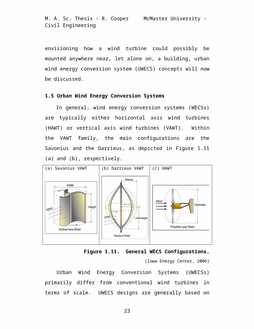
1.5 Urban Wind Energy Conversion Systems
In general, wind energy conversion systems (WECSs)
are typically either horizontal axis wind turbines
(HAWT) or vertical axis wind turbines (VAWT). Within
the VAWT family, the main configurations are the
Savonius and the Darrieus, as depicted in Figure 1.11
(a) and (b), respectively.(a) Savonius VAWT (b) Darrieus VAWT (c) HAWT
Figure 1.11. General WECS Configurations.(Iowa Energy Center, 2006)
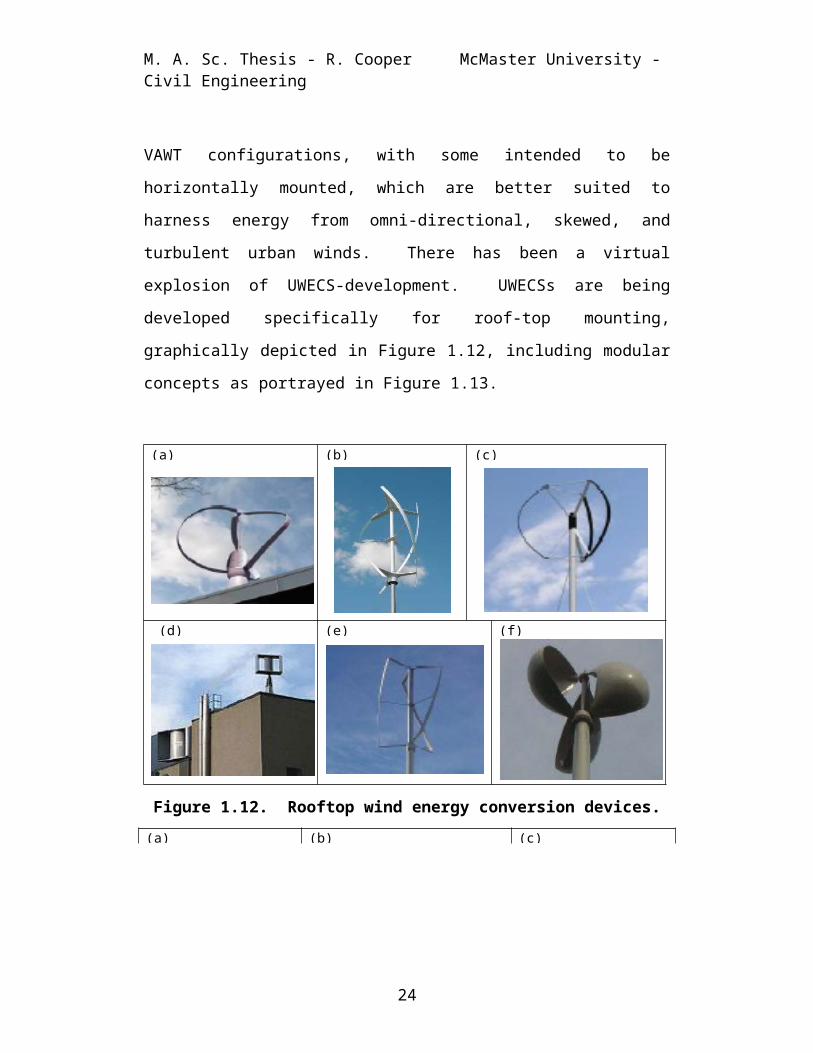
Urban Wind Energy Conversion Systems (UWECSs)
primarily differ from conventional wind turbines in
terms of scale. UWECS designs are generally based on
23
M. A. Sc. Thesis - R. Cooper McMaster University - Civil Engineering
VAWT configurations, with some intended to be
horizontally mounted, which are better suited to
harness energy from omni-directional, skewed, and
turbulent urban winds. There has been a virtual
explosion of UWECS-development. UWECSs are being
developed specifically for roof-top mounting,
graphically depicted in Figure 1.12, including modular
concepts as portrayed in Figure 1.13.
(a) (b) (c)
(d) (e) (f)
Figure 1.12. Rooftop wind energy conversion devices.(a) (b) (c)
24

M. A. Sc. Thesis - R. Cooper McMaster University - Civil Engineering
(d) (e)
Figure 1.13. Modular Rooftop modular wind energyconversion devices.
The reader is directed to the photomontage matrix in
Appendix K for details pertaining to WECS type,
manufacturer, and image credits related to Figures 1.12
- 1.14, inclusive.
Configurations exploiting BAWT theory are roof-
mounting (Figure 1.14 (a)), ground-mounted near
buildings (b), or integrated into a building, as is the
case in the recently constructed Bahrain World Trade
Center in Figure 1.14 (c) and the University of
Strathclyde's ducted wind turbine (d).
(a) (b)
25

M. A. Sc. Thesis - R. Cooper McMaster University - Civil Engineering
(c) (d)
Figure 1.14. Building augmented wind energy conversionsystems.
Excellent reviews of the BUWT industry, including
concepts, research, and current manufacturers are
provided by Blanch (2002) and Wineur (2007). A
comprehensive tabulation of more than 60 WECSs
developed throughout Europe and North America,
including BUWT-potential and performance
26

M. A. Sc. Thesis - R. Cooper McMaster University - Civil Engineering
characteristics, has been compiled by Dutton et al.
(2005). The scope and objectives of this research
undertaking will now be discussed.
1.6 Scope and Objectives of the Research Undertaking
The recent privatisation of various sectors of the
utilities industry, namely natural gas and electricity,
has created supposedly beneficial-to-the-customer
competition amongst the various providers. But the end
result is that the consumer must now deal with the
worry about the future viability of the chosen provider
and continually ‘do the numbers’ to ensure that s/he is
getting the best price. Insecurity, especially in
light of the blackout of 2003, and concern about cost,
prevails. Given the current climate, literally,
politically, and economically, this is an ideal time to
give the security of energy supply and financial
control back to the building owner.
What if one could produce a large portion of their
energy needs right on their own property? The
questions that need to be answered would include:
What is the site's renewable energy (RE) potential(e.g., wind and solar energy generated)?
What efficiency, cost, etc. can be expected of thevarious RE extraction devices?
27

M. A. Sc. Thesis - R. Cooper McMaster University - Civil Engineering
Where is the optimal placement for RE extraction devices?
What are the implications of site layout on RE energy potential?
What is the effect of building configuration on REpotential?
Could individual architectural features enhance REpotential?
What is the efficiency of the dwelling? What is the energy demand incurred by the
building's occupants? What is the estimated energy surplus / deficit? What are the various energy storage options? What are the current and projected utility costs? When will payback be realised?
The scope of this research undertaking proposes to
address assessment of the potential wind energy,
optimal placement and scale of UWECSs, and the
implications of building aerodynamics-induced wind
amplification. Evaluation of other RE sources,
dwelling efficiency, energy demand, and various socio-
economic aspects can be conducted using existing
applications. The reader is directed to Appendix L to
view a matrix of tools supporting such evaluations.
The main objectives of this research are:
Development of a prototype urban wind energy planning (UWEP) decision support system (DSS) for
28

M. A. Sc. Thesis - R. Cooper McMaster University - Civil Engineering
homeowners, urban designers or planners, architects, and UWECS developers;
Assessment of building aerodynamics-induced wind amplification;
Assessment of the seasonal variation of the wind resource; and
Determination of optimal UWECS placement.
In accordance with the objectives and underlying
motivation behind this research undertaking, this
Thesis primarily documents the development of a
prototype urban wind energy planning (UWEP) decision
support system (DSS). It includes a first attempt
approach at estimating building-aerodynamics induced
wind amplification dependent on neighbourhood
characteristics, meteorological conditions, and a
subject building. The UWEP DSS will support wind
energy potential assessment of both an existing and a
proposed building, by providing the capability to make
various building feature-related changes (e.g., roof
type and pitch) in an iterative fashion. It will be
capable of conducting a mean annual as well as a
seasonal or monthly assessment. The proposed tool will
link the user to various online applications and
databases, thereby requiring a minimal amount of user
knowledge concerning meteorology, geography, or
29

M. A. Sc. Thesis - R. Cooper McMaster University - Civil Engineering
building aerodynamics. The UWEP DSS will inform the
user on the:
potentially amplified mean wind speeds at the site,
potential energy that could be extracted, approximate size of an appropriate UWECS, placement location most appropriate for the
subject site, and months with the greatest potential.
1.7 Thesis Structure
This Thesis is divided into the following six
chapters:
Chapter 1 - Introduction Chapter 2 - Literature Review Chapter 3 - Conceptual Model Development Chapter 4 - Decision Support System Development Chapter 5 - Application of the Decision Support
System Chapter 6 - Summary, Conclusions, and
Recommendations
Following this introduction, Chapter Two of the Thesis
is devoted to a literature review, which draws from
numerous interrelated disciplines to explore the
feasibility of BAWT theory in an urban setting. This
chapter includes a review of the current state of the
relatively new field of wind power meteorology, related
30

M. A. Sc. Thesis - R. Cooper McMaster University - Civil Engineering
fields of research in support of defining the flow-
field in the building affected zone, and an overview of
the various applications and DSSs currently in
existence. Chapter Three details the development of
the conceptual model of the proposed UWEP DSS. The
fourth chapter details the development of the UWEP DSS
based on the conceptual model. This chapter includes
discussion on the form, function, and theory behind the
mathematical computations of the proposed tool.
Chapter Five contains a discussion on the performance
of, and results produced by, the UWEP DSS when applied
to case studies. Finally, in Chapter Six, a summary of
the research undertaking is provided, including
conclusions and recommendations for future research.
31

M. A. Sc. Thesis - R. Cooper McMaster University - Civil Engineering
2 LITERATURE REVIEW
Recognising the highly interdisciplinary nature of
this research, an extensive manual and electronic
search was conducted. Initially, an internet search
was performed to identify the various national and
international institutions, organisations, and
associations advocating wind energy. The World Wide
Wind Energy Association (WWEA) (2006) created in 2001
and the Global Wind Energy Council (GWEC) (2007)
established in early 2005, were identified as key
organisations providing a forum for this truly
international pursuit. Even though there is an
overwhelming amount of published information and
ongoing research activity, completed and planned
installations are largely based on the traditional
approach to wind energy extraction, namely through wind
farms and stand-alone rural towers. It was through the
European Wind Energy Association (EWEA) that Project
WEB (Wind Energy for the Built Environment), funded in
part by the European Commission (EC) in the framework
of Joule III, was identified.
Having identified the disciplines and key concepts,
a search of Journals and Conference Proceedings was
conducted through McMaster University’s online
32

M. A. Sc. Thesis - R. Cooper McMaster University - Civil Engineering
Information Portal known as Morris. Databases such as
INSPEC, Science Citation Index, Compendex, SAGE Full-
Text Collection, etc., accessed through Scholars
Portal, Web of Knowledge, and Engineering Village 2,
identified the following key journals:
Atmospheric Environment, Boundary-Layer Meteorology, Energy and Buildings, Energy Conversion and Management, Environment & Urbanisation, Journal of Applied Meteorology, Journal of Wind Engineering, Journal of Wind Engineering and Industrial
Aerodynamics, ReFocus, Renewable Energy, Theoretical and Applied Climatology, Wind & Structures, Wind Energy, and Wind Engineering.
To develop the structure of the proposed Decision
Support System (DSS), regulations, codes, standards,
and guides pertaining to wind turbine siting and
building construction were reviewed. Several articles
pertaining to decision support regarding other
renewable energy sources were also assessed.
33

M. A. Sc. Thesis - R. Cooper McMaster University - Civil Engineering
Additional information was found in various trade
magazines (e.g., North American Wind Power, Wind
Directions, HomePower, and Popular Mechanics). Not
surprisingly, comments by organisations countering wind
energy industry initiatives (e.g. Industrial Wind
Action Group (IWA) (2006)) provided the impetus and
encouragement to pursue unconventional means for wind
energy extraction.
Finally, several software applications and online
assessment tools were explored to determine their
applicability and to further develop the methodology of
the proposed DSS.
2.1 The Interdisciplinary Nature of this Research
The wind in urban and suburban areas is a field of
study of, and interest to, many applied sciences (e.g.
climatology and meteorology, bioclimatic design and
building physics, pollutant dispersion studies, urban
and landscape planning, etc). It is only in the last
10+ years that findings from the field of agricultural
and forest meteorology have been explored for their
applicability to the built environment. Starting with
the formulation of the Urban Heat Island (UHI) concept
by Oke (1978), research proceeded to further
exploration of the correlation between meteorological
34

M. A. Sc. Thesis - R. Cooper McMaster University - Civil Engineering
conditions and the morphological and anthropogenic
impact of urban/suburban developments.
The organisation of this literature review is based
on these interdisciplinary correlations and best
summarised using building blocks, as illustrated in
Figure 2.1.
Modelling, including Global Information
Systems (GIS)
Planning
Urban, inc
luding
landscape
Energy Managem
ent & Pow
er Transmission
Decision Support System(DSS)
Energy SciencesSystem s
ConservationAlternatives
Fluid Dynam ics
BuildingAerodynam ics W ind Engineering
Turbom achinery
Energy Conversion
EngineeringCivil
M echanicalAerospaceElectricalChem ical
Atm ospheric SciencesM eteorologyClim atologyW eather
Sustainable
Urban Boundary Layer
Renewable
W indSolarEtc.
Roughness
Resources
Building SciencesEnergy M anagem entResource M anagem ent
ArchitecturalBuilt Environm ent … . Passive & Low Energy
Environm ental SciencesUrban Environm entPollution DispersionG lobal Change
Im pact Assessm ent
Alternative Energy
Geographic
Information
Syste
m (GIS)
Canopy Layer
EcologyForestryAgricultureGeographyTopography
i.e.Orography
G lobal Political Econom yEco-Socialism
Energy & Resource Policies … Building Codes & Legislation … Incentives & Research Funding
Computer Science
Figure 2.1. The interdisciplinary blocks of urban windenergy research.
The foundation is the field of atmospheric
sciences. Looking to the lower right hand quadrant in
Figure 2.1, geography & ecology are seen as the first
fields to explore earth-atmosphere interactions.
Contributions from these fields include development of
35

M. A. Sc. Thesis - R. Cooper McMaster University - Civil Engineering
the geographic information system (GIS), the concept of
roughness, and the definition of a canopy layer, upon
which the concept of the urban canopy layer (UCL) is
based. The interdisciplinary fields of energy,
environmental, and building science combine various
engineering disciplines under the influence of these
concepts and developments. Ideally, the field of
architecture should encompass the whole.
The core group of disciplines, indicated by the
dot-shaded region within the building block model in
Figure 2.1, is then regulated by the global political
economy and organised through various planning
disciplines. Finally, it is the contributions from the
field of computer science that provide the practitioner
with tools and decision support systems to be able to
put the entirety of this body of knowledge into
application.
Due to the interdisciplinary nature of the research
undertaking and the intrinsic connection between urban
morphology and the local climate, new concepts often
need to be introduced in one section while detailed
discussion thereof is withheld until a later section.
That said, the structure of the literature review
attempts to build background as it proceeds, while
36

M. A. Sc. Thesis - R. Cooper McMaster University - Civil Engineering
reserving detailed discussion to concepts that pertain
directly to the proposed DSS. It is divided into the
following main sections:
Wind Power Meteorology Overview; The Urban Boundary Layer (UBL), including
modelling; Wind Atlases; Wind Atlas Methodology (WAM); Wind Resource Assessment; The Built Environment; and Decision Support Systems (DSS).
2.2 Wind Power Meteorology Overview
Wind power meteorology is an applied science,
founded in boundary layer meteorology and based on wind
climatology and geography, specifically focussed on
wind resource assessment to optimise wind energy
conversion system (WECS) placement (Petersen,
Mortensen, Landberg, Højstrup, & Frank, 1998a). The
'klimatope' (landscape climate) in Figure 2.2 provides
an illustrative portrayal of this combination of
geographic, land-use, and climatic elements (Tanaka &
Moriyama, 2005). The climate analysis map includes
arrows indicating the direction of the regional land
and sea breezes, radar plots identifying locally
observed wind direction by frequency and cardinal
37

M. A. Sc. Thesis - R. Cooper McMaster University - Civil Engineering
sector, and colour-coded dots indicating mean
temperatures.
Figure 2.2. The Osaka City 'klimatope'.Extracted from the prototype of overlaid “Climate Analysis Map” of
Osaka City (Tanaka & Moriyama, 2005).
Wind climatology, based on planetary boundary layer
(PBL) meteorology, deals primarily with the
geographical and temporal distribution of the wind
regime, including both speed and direction. The PBL is
the layer of the atmosphere at the bottom of the
troposphere where both mechanical and thermal processes
occur. A short primer on PBL meteorology is provided
in Appendix A, while terminology is defined in the
Glossary, for the reader seeking more background. This
38

M. A. Sc. Thesis - R. Cooper McMaster University - Civil Engineering
review will focus on the urban boundary layer (UBL)
within the PBL.
The geophysical components of interest are the
terrain topography (including vegetation, built-up
areas, and soil and water surfaces, known as roughness
elements) and the orography or large-scale terrain
features (including hills, cliffs, ridges, escarpments,
and valleys). The retardation effect of the size and
distribution of these surface features on the wind near
ground level is mathematically represented by a
roughness length [z0] parameter (Petersen, et al.,
1998b).
The rudimentary fundamentals of the climatological
aspects of this discipline are covered in the following
sections.
2.3 The Urban Boundary Layer
The urban boundary layer (UBL) is modelled as
either an internal boundary layer (IBL) of the PBL
(Fisher et al., 2004; L. Landberg & Watson, 1994;
Verkaik & Smits, 2001) or as a two-layer PBL (Clarke &
Hess, 1974; Verkaik & Smits, 2001; Verkaik, 1999).
Figure 2.3, based on the earlier works of Oke (1978),
appears in numerous articles by fellow researchers,
representing the most widely recognised and accepted
39

M. A. Sc. Thesis - R. Cooper McMaster University - Civil Engineering
conceptual structure of an unstable daytime UBL. The
boundary layer is considered to be unstable during the
day while the surface is transferring heat to the
atmosphere and stable at night when the heat transfer
is reversed. The addition of a height scale attempts
to add clarity to the notes, including the designation
of the PBL height [zi] ~ u*/f (Verkaik & Smits, 2001;
Clarke & Hess, 1974). The average height of the
roughness elements [zH] is assumed to represent the
approximate height of the urban canopy layer (UCL),
with the term canopy pertaining to a group of roughness
elements. The height of the roughness sublayer (RSL)
[z*] is equated to a zH; where 2 < a < 5 (Fisher et
al., 2004). The inertial sublayer (ISL) lies roughly
between z = a zH and 0.25, where is the boundary-
layer height (MacDonald, 2000 after (Raupach et al.,
1980)). The top of the UBL is designated as or h.
In Figure 2.3 c) the sky view factor (SVF) is used to
define street canyon width-to-height ratio and an
idealised canyon vortex is illustrated. As illustrated
in Figure 2.3, the UBL can be broadly stratified into
mesoscale, local scale, and microscale layers, in order
of increasing complexity and resolution.
Defining the extents and properties of these layers
is crucial to wind power meteorology for estimation of
40

M. A. Sc. Thesis - R. Cooper McMaster University - Civil Engineering
mean wind speed as a function of height and terrain-
induced roughness. Boundary layer theory (i.e., the
two-layer and the IBL) defines how to estimate this
mean wind speed profile within various layers of the
UBL.
a) M esoscale
RURAL
b) Local scale
z
SUBURBAN
c) M icroscale
URBAN
U C L
Inertial Sublayer
Roughness Sublayer
zH
z*
UC L
Urban Boundary Layer
W ind Direction
)z(u
PBL
Surface Layer
Outer Layer
SVF
Surface Layer
Figure 2.3. Urban boundary layer structural sketch.Based on Fisher et al. (2004) and Rotach et al. (2004), modified
after Oke (1987).
The IBL theory is based on well-defined upwind and
downwind roughness transitions, such as the rural
41

M. A. Sc. Thesis - R. Cooper McMaster University - Civil Engineering
through suburban to urban in Figure 2.3 a), which
modify the wind regime as it passes through. Figure
2.4 below further serves to illustrate the effect of
terrain roughness on the mean wind speed profile. It
is proposed within the literature that turbulent
kinetic energy (TKE) is what facilitates mean wind
speed adaptation and/or adjustment to substantially
different terrain (e.g., open country vs. a small town)
(Chan, 2001).
34 m /s
14 m /s
W oodland / Sm all Town
150 21 m /s
225 30 m /s
City Centre Open Country
Height [z] (m
)
75 32 m /s20 m /s
29 m /s
36 m /s
38 m /s
300
)z(u
Figure 2.4. The terrain dependent velocity shearprofiles.
Terrain roughness decreases from left to right (i.e., from CityCentre to Open Country). Modified after Dalgliesh & Boyd (1962).
This original approach worked well when applied to
vegetative stands (e.g., crops or forest) but does not
42

M. A. Sc. Thesis - R. Cooper McMaster University - Civil Engineering
have the two-layer model's advantage of being able to
deal with the multiple roughness transitions typical of
an urban surface. (van Kuik & Bierbooms, 2005 p. 47)
The IBL model cannot accommodate multiple transitions
due to the fetch associated with each roughness region,
which is often longer than the distance between
transition zones (e.g., urban-to-suburban in Figure 2.3
a). The fetch is the horizontal distance required for
the wind profile to adjust to the new roughness. To
address this deficiency, some attempts have been made
to imbed individual IBL models within an IBL model
(Belcher, Jerram, & Hunt, J. C. R., 2003). Models
considering only the surface layer are also called
surface layer (SL) models (e.g., COAST (Verkaik,
1999)). In wind power meteorology, IBL theory is
applied to determine orographic terrain-induced
accelerations.
In the two-layer UBL conceptualisation, the
vertical structure is comprised of a surface layer (ISL
+ RSL) and an outer (mixed) layer (Figure 2.3 a)).
Over urban surfaces the upper and lower limits of the
inertial sublayer (between z/z0 >>1 and z/u* <<1) are
thought to coincide (Rooney, 2001). Two-layer theory
does not factor in orographic terrain-induced
43
M. A. Sc. Thesis - R. Cooper McMaster University - Civil Engineering
accelerations. The theory behind this approach will be
covered in Section 2.6.
The past two decades of extensive research
involving the UBL has resulted in numerous advances in
boundary layer climatology, including a better
understanding of the roughness sublayer (RSL)
(Arnfield, 2003). As the research focus has shifted to
the development of numerical models, improved methods
of evaluating the crucial parameters (e.g., roughness
length [z0]) from urban form, methods of linking
microscale to mesoscale urban climate work, and model
validation are required. To decrease uncertainty,
careful consideration of spatial and temporal relations
is recommended. (Şahin, 2004)
Numerical models are based on the two-layer UBL
theory, the IBL theory, or a combination of the two.
UCL modelling, for the most part, will be covered in
Section 2.8 though some overlap is unavoidable. It is
within the UCL that urban-type roughness elements
induce complex turbulence fields and localised speed-
ups, which are of greatest importance to this research
undertaking. This section of the literature review
will focus primarily on defining the wind climate.
44

M. A. Sc. Thesis - R. Cooper McMaster University - Civil Engineering
2.3.1 The Wind Climate
Wind is a complex, three-dimensional phenomenon
generated by large scale pressure differences caused by
the unequal distribution of solar radiation affected by
both thermal (Souch & Grimmond, 2006) and mechanical
processes. In wind power meteorology, interest
primarily lies in an assessment of the implications of
mechanical processes on the horizontal component of the
wind speed vector. The wind speed is also a function
of the local climate (hence year, time of year, and
time of day). Time series data (TSD) for the
horizontal component of wind speed and the associated
direction are available through most national
meteorological organisations. In Canada, national
climate data are available online through the National
Climate and Information Archive (EC, 2005d).
In order to apply the boundary layer theory, an
accurate representation of the wind climate, including
temporal variation (Table 2.1) and frequency
distribution must be developed.
Table 2.1. Causes and time scale of temporal wind
variation.
45

M. A. Sc. Thesis - R. Cooper McMaster University - Civil Engineering
Cause Tim e ScaleGusts (e.g. turbulence) Sub-second to secondDiurnal cycle DayInversion layers Hour(s)W eather patterns Hours to daysSeasonal cycle (e.g. m onsoon) SeasonalAnnual variation Years
(Ackermann & Söder, 2000) The inversion layer is explained inAppendix A. †Discussion on turbulence is reserved for Section 2.8.
Studies concerning temporal variability (Li & Li,
2005a) have been conducted, investigating diurnal
(Weisser & Foxon, 2003), seasonal (T. Chang, Wu, Hsu,
Chu, & Liao, 2003; Lun & Lam, 2000), and inter-annual
(Voorspools & D’ haeseleer, 2007) time scale
implications. Temporal variability in wind direction
is considered negligible, except in coastal regions
where land-sea breezes are prevalent (Dandou, Tombrou,
Akylas, Soulakellis, & Bossioli, 2005).
To account for inter-annual variation, thereby
minimising the impact of the so-called 'windy years'
(the 90's), a full set of chronological data spanning
at least 30 years is recommended (van Kuik & Bierbooms,
2005). Alternatively, analysis based on one year of
data has been proven to yield predictions accurate to
within 10% (Jamil, Parsa, & Majidi, 1995 p. 623).
Compared to a rural environment, the influence of
seasonal variation within the UBL is reduced due to
46
†

M. A. Sc. Thesis - R. Cooper McMaster University - Civil Engineering
roughness-induced wind field modifications (Radics,
Bartholy, & Pongrácz, 2002).
To reduce the computational effort required to take
into account temporal variation, the development of a
compressed (COM) wind data set is proposed (Celik,
2003). COM is currently available for solar radiation,
representing the important statistics of an entire
month using less than a month's worth of data. Another
useful data summary tool is the test reference or
meteorological year (TRY/TMY). Figure 2.5 illustrates
the (a) monthly and (b) diurnal variation of the mean
wind speed, comprised of instantaneous wind
measurements, of three different wind regimes.
(a) (b)
Figure 2.5. Variation of the primary northern hemisphere wind climates.The magnification portion shows the actual instantaneous wind measurements from which the mean is calculated. Modified after Petersen et al. (1997) p. 12.
47

M. A. Sc. Thesis - R. Cooper McMaster University - Civil Engineering
On closer examination of the instantaneous wind
measurements, highlighted by the magnifying glass in
Figure 2.6 (b) above, the mean and turbulent components
can be seen (as illustrated below). Turbulence, or
gustiness, is generally three-dimensional and defined
as any irregular velocity perturbation superimposed on
the mean. Turbulence can be mechanically and/or
thermally induced, through what are called ground
forcings. The primary mechanical forcings are
frictional drag (i.e., terrain-induced roughness and
form drag, e.g. flow deflection around obstacles,
including orographic terrain features (Roulet, 2004)).
Thermal forcings are primarily due to solar heating of
the ground and buildings, which causes the air in
contact to become warmer than the surrounding air mass,
generating buoyancy-induced thermals.
48

M. A. Sc. Thesis - R. Cooper McMaster University - Civil Engineering
Figure 2.6. The components of the instantaneous windspeed.
(Stull, 1988)
It is due to turbulent momentum flux (i.e.,
Reynolds stress) that the effect of the ever changing
surface forcings is transmitted throughout the boundary
layer (Stull, 1988). In wind power meteorology, a
turbulence intensity factor (TI), based on the standard
deviation of the wind speed, is the most commonly used
indicator of turbulence (Singh, Bhatti, & Kothari,
2006). In boundary layer meteorology, turbulence
kinetic energy (TKE) is used to more fully define the
variance. The reader is directed to the works of
Petersen et al. (1998a) and Stull (1988) for additional
detail.
Wind power meteorology relies on the friction
velocity [u*] parameter for the mathematical
representation of Reynolds stress in the formulation of
the wind profile as a function of terrain-induced
roughness and height, which is discussed in Section
2.6.
2.3.2 Frequency Distributions
While temporal variation is concerned with the
variability of the mean over a specific time period,
49

M. A. Sc. Thesis - R. Cooper McMaster University - Civil Engineering
frequency distributions are used to define the
probability of observing specific wind directions and
speeds about the mean. Referring back to Figure 2.5,
Figure 2.7 below illustrates the wind speed frequency
distributions associated with the same three wind
climates.
Figure 2.7. Northern hemisphere wind climate frequencydistributions.
Extracted from Petersen et al. (1997) p. 12.
The frequency of the wind direction is typically
portrayed in a wind rose, which illustrates frequency
by directional sector. Wind is inherently multi-
directional, but the wind direction at a particular
location can usually be considered as predominantly bi-
50

M. A. Sc. Thesis - R. Cooper McMaster University - Civil Engineering
directional, and occasionally uni-directional as
illustrated in Figure 2.8.
0.0%5.0%10.0%15.0%20.0%25.0%
N
NNE
ENE
E
ESE
SSE
S
SSW
W SW
W
W NW
NNW
Figure 2.8. The Toronto Island airport wind directionrose of June 2005.
The wind speed frequency distribution is portrayed
in histogram form and/or a representative probability
density function (pdf). Histogram bins are often based
on wind speed class, a predefined classification system
representing wind speed ranges (e.g., the Beaufort
scale (University of the Southern Pacific, & UNESCAP,
2004)).
Extensive research has been conducted fitting time-
series wind speed data to pdfs, primarily the log-
normal, Rayleigh (Li & Li, 2005b), and Weibull (Nigim &
Parker, 2007; Jamil et al., 1995; Seguro & Lambert,
2000) distributions. The two-parameter Weibull
51

M. A. Sc. Thesis - R. Cooper McMaster University - Civil Engineering
distribution, below, has been found to yield the most
accurate estimation of the wind speed distribution:
Frequency; (2.1)
where: u is the horizontal wind speed, k is the shape
parameter, and c is the scale parameter. Further
detail regarding the Weibull pdf, including the double-
peaked, bi-Weibull distribution, can be found in
Burton, Sharpe, Jenkins, & Bossanyi (2001).
2.4 Boundary Layer Modelling
The defining equations of boundary layer theory are
the Navier-Stokes equations, which are derived from the
basic principles of conservation of mass, momentum, and
energy. Due to the highly non-linear nature of
atmospheric phenomena within the UBL, numerical models
are used to explicitly or implicitly solve the defining
equations. These models are typically either based on,
or validated by, field observations. Wind tunnel
testing (scale-modelling) appears to be reserved for
the assessment of the complexities associated with the
UCL and terrain orography. Over the last 20 years,
computers have allowed for the development of powerful
numerical models based on the theory developed by
earlier researchers. Much of the current research is
52

M. A. Sc. Thesis - R. Cooper McMaster University - Civil Engineering
focussed on improving the accuracy and increasing the
resolution of these numerical models, while reducing
computational effort.
A simplified classification of meteorological
models, Table 2.2, is provided by Petersen et al.
(1998b). Models are actually comprised of a
combination of these classifications (e.g., MC2 is a
non-hydrostatic, linear, diagnostic, mesoscale,
neutral, turbulent closure model). Complexity
generally increases from left to right in the below
tabulation.
Table 2.2. Broad-scale classification of
meteorological models.Classifica ComplexityDynamics kinematic (mass-consistent), Advection linear, non-linear.Time diagnostic, prognostic.Spatial Global (synoptic), mesoscale > 5 km, Stratifica neutral, non-neutral.Friction frictionless, turbulent closure.Formulatio analytical, spectral, grid point.Type flow model, wind climate model.
Modified after Petersen et al. (1998b) p. 65. † verticalacceleration is considered negligible compared to vertical
pressure gradients and vertical buoyancy forces, which typifies athermally vs. mechanically-driven process. Global scale is
typically in the order of > 100 km.
Models are generally discussed in terms of their
spatial scale, also referred to as resolution.
53

M. A. Sc. Thesis - R. Cooper McMaster University - Civil Engineering
Regional numerical weather prediction (NWP) models are
classified as mesoscale. The most common mesoscale
models used in wind power meteorology are:
Karlsruhe Atmospheric Mesoscale Model (KAMM) - theUniversity of Karlsruhe,
5th generation Mesoscale Model (MM5) - Penn State/NCAR
Mesoscale Compressible Community (MC2) model - MSC,
HIgh Resolution Limited Area Model (HIRLAM) - the European Meteorological Institute, and
Mesoscale Atmospheric Simulation System (MASS) - Meso Inc.
(van Kuik & Bierbooms, 2005)
Unfortunately, a Unix workstation or a Linux-based PC
is required to run these models, in addition to a
thorough understanding of meteorological processes and
the associated parameterisation schemes.
As the aim of this literature review is to provide
a reasonable background for the scope of the associated
research, only a condensed description of the relevant
mesoscale and microscale models on which wind atlases
and associated commercial software development are
based will be provided, highlighting key findings and
limitations.
54

M. A. Sc. Thesis - R. Cooper McMaster University - Civil Engineering
2.4.1 Mesoscale Models
Mesoscale models (A. Martilli, Clappier, & Rotach,
2002) (e.g., Geesthacht Simulation Model of the
Atmosphere (GESIMA) (Mengelkamp, 1999)) are typically
bounded by large-scale climatological parameters (e.g.,
reanalysis data) and use a statistical-dynamical
downscaling procedure (Frey-Buness, Heimann, & Sausen,
1995) to calculate the regional wind climate. The two
main international models are the MM5 and the MC2. The
NCAR series of MMx models, particularly the MM5, and
the MSC's MC2 are both non-hydrostatic models, which
became available at about the same time, in the mid-
1990's (Benoit et al., 1997).
The foundation of the Canadian wind atlases is the
MC2 model. It was developed in the mid-1980s at MSC-
RPN (Recherche en Prévision Numérique) and the
Université du Québec à Montréal (UQAM) (EC, 2005c).
Benoit et al.'s (1997) work documents the developmental
research and early results of the MC2. It is governed
by the fully compressible Euler, or Navier-Stokes,
equations, which include the full time derivatives of
all three components of velocity. “It is probably the
only currently available 3D fully compressible model
55

M. A. Sc. Thesis - R. Cooper McMaster University - Civil Engineering
that uses a semi-implicit semi-Lagrangian (SISL) time
scheme” (Benoit et al., 1997 p. 2382).
Over the last decade these models have been used in
numerous bodies of interdisciplinary research (e.g.,
pollutant dispersion studies by Tong, Walton, Sang, &
Chan (2005) and anthropogenic impact studies by Pino,
Vila-Guerau De Arellano, Comeron, & Rocadenbosch (2004)
and Dandou et al. (2005)). These studies have served
to validate the models and to identify their
limitations. The authors emphasise the importance of
accurate boundary conditions and suggest that some of
the inaccuracies may be attributed to very local
effects unresolved by model resolution. Resolution
improvements can be achieved by imbedding a UCL model,
typically referred to as an urban parameterisation
scheme (to be addressed in Section 2.8.2), into the
mesoscale model (Dandou et al., 2005; Tong et al.,
2005) or by using a microscale model. The reader is
directed to the previously cited references for more
in-depth information pertaining to the theory behind
the models.
2.4.2 Microscale Models
While mesoscale models define the regional wind
regimes, the increased horizontal resolution of
56

M. A. Sc. Thesis - R. Cooper McMaster University - Civil Engineering
microscale models can take the effects of complex
surfaces on the local flow field into consideration.
These models require meteorological data, typically
generated by mesoscale models and provided as
microscale model boundary conditions, as well as
geophysical data. The geophysical data are extracted
from digital elevation models (DEM), Shuttle Radar
Topographic Mission (SRTM) data, and/or land cover and
topographic databases.
In the field of wind power meteorology, the
microscale models, specifically developed to assess the
local wind climate, are most often imbedded in the
associated application software (see Section 2.7).
Examples of microscale models include the Riso
Laboratory of Denmark's Wind Atlas Analysis and
Application Program (WAsP) (Petersen et al., 1998b),
Environment Canada's MS-Micro (Walmsley, Taylor, &
Keith, 1986), and WindMAP (based on MC2).
Computational fluid dynamics (CFD) models, or wind flow
solvers, based on Reynolds Averaged Navier-Stokes
(RANS) equations (e.g., WindSim) are also used for
microscale assessment.
MS-Micro, developed through a partnership between
MSC and Zephyr North, specifically analyses steady-
57
M. A. Sc. Thesis - R. Cooper McMaster University - Civil Engineering
state flow over complex terrain. MS-Micro/3, the
latest version of the linear 3D MS3DJH/3R numerical
flow model (Walmsley et al., 1986), employs the two-
layer UBL model theory to calculate roughness-change
induced flow modifications without requiring “that the
wind data be taken upstream of the site of interest”
(Jacobson & Malte, 2005 p. 11). MS-Micro is only
capable of modelling the steady-state and neutrally
stratified boundary layer over gentle mountainous
terrain without flow separation. For more rugged
terrain and non-neutral atmospheric stratification,
other microscale models must be used (Scholtz & Liu,
2005).
2.4.3 Model Combinations
As a precursor to the modern day wind atlas, one of
the first applications of combined models was in
forecasting the weather. In wind power meteorology,
weather forecasting is a critical component of wind
farm production prediction. The flow chart in Figure
2.9 depicts the components of Zephyr/Predictor (Giebel
& Risø National Laboratory, 2006), a wind farm
production-prediction system, combining mesoscale and
microscale models.
58

M. A. Sc. Thesis - R. Cooper McMaster University - Civil Engineering
Figure 2.9. Flow chart of the Riso wind powerprediction model.
The boxed-in regions represent the mesoscale generation of thesurface or regional wind climate (solid line) and the microscale
generation of the local wind climate (dashed line). Modified afterPetersen et al. (1998b p. 68).
One of the main challenges in numerical modelling
comes from having to weigh computational effort (i.e.,
time to model convergence) against accuracy and/or
resolution. By combining NWP, mesoscale, and
microscale models, optimised for a specific scale or
type of complexity, accuracy and resolution can be
retained without adversely affecting convergence. The
integration of these three types of models has not yet
59

M. A. Sc. Thesis - R. Cooper McMaster University - Civil Engineering
been perfected, but software along these lines has been
developed and proven to yield more accurate results
(Section 2.7.2). (Jacobson & Malte, 2005) The wind
atlas methodology (WAM) used to create wind atlases is
an example of just such an integration.
Wind atlases represent the outcome of the first
stage (i.e., the development of the regional wind
climate (Figure 2.9 - solid-line boxed region)) or the
first two stages (i.e., the development of the local
wind climate (Figure 2.9 - dashed-line boxed region)),
as illustrated above.
2.5 The Wind Atlas
Creation of a wind atlas, a systematic and
comprehensive collection of regional wind climates
(RWC) (Mortensen, 2007), is typically based on the
mesoscale-portion of the WAM, as delineated in Figure
2.9 above. As such, differentiation is made between
wind data, a wind atlas, and wind resource assessment
(see Section 2.7) (Landberg et al., 2003).
In general, the methodology extrapolates detailed
information about the mean wind climate from one
location to another. The Risø National Laboratory
proposes two main methodologies: the observational wind
atlas (OWA) methodology, based on data collected at
60

M. A. Sc. Thesis - R. Cooper McMaster University - Civil Engineering
numerous meteorological stations (Mortensen, 2006) and
the numerical wind atlas (NWA) methodology, based on
mesoscale modelling and a reanalysis data set
(Mortensen, 2006a). Though wind mapping began in the
early 1970s, this review will focus on the Canadian
Wind Energy Atlas and the Ontario Wind Resource Atlas,
both based on NWA methodology. A summary table of the
primary features of these and other atlases is provided
in Appendix B.
The Wind Energy Resource Atlas of the United States
(US) was developed in the late 1970s by Pacific
Northwest Laboratory (PNL) in support of the Federal
Wind Energy Program's aim to assess the nation’s wind
resource. Figure 2.10 indicates the twelve regions for
which wind energy atlases were produced using a wide
variety of data and analysis techniques. Each region
is divided into its individual states (Figure 2.10),
while each state is further subdivided into grid cells
as follows: 1/4° latitude by 1/3° longitude (in the
contiguous US), 1/2° latitude by 1° longitude (in
Alaska), and 1/8° latitude by 1/8° longitude (in
Hawaii, Puerto Rico, and the Virgin Islands).
61

M. A. Sc. Thesis - R. Cooper McMaster University - Civil Engineering
Figure 2.10. Wind Energy Resource Atlas of the UnitedStates.
The 12 regions are outlined in bold and the individual states indashed lines (National Renewable Energy Laboratory (NREL), 1986).
The digitised maps provide mean wind speeds and
power densities at heights of 10 m and 50 m (Figure
2.11). Though seasonal mapping was conducted, no
consideration was given to orographic terrain-induced
variability.
62

M. A. Sc. Thesis - R. Cooper McMaster University - Civil Engineering
Figure 2.11. Analyzed Winter Season Average WindResource Maps.
(NREL, 1986)
Detailed maps provide mean wind speed and wind
power density by class at a height of 50 m (Figure 2.12
(a)). Low resolution topographical maps are provided
at both the region and individual state level (Figures
2.12 (b) & (c)). At the individual state level, only
wind power class contour intervals are depicted (Figure
2.12 (c)).
63

M. A. Sc. Thesis - R. Cooper McMaster University - Civil Engineering
(a) Winter wind power classifications
Figure 2.12. Wind resource estimates in the Northwestregion of the US.
In a) shaded regions identify power classifications @ 50 a g.l.while the legend provides the associated wind power density and
speed (NREL, 1986). A dynamic map is available in the form of theNew York Wind Resource Explorer, powered by Wind Resource
Explorer (AWS Truewind, 2004a).
64
(b) Geographic map of Northwest region
(c) New York state average annual wind power density by class

M. A. Sc. Thesis - R. Cooper McMaster University - Civil Engineering
This atlas is one of the few to include wind
resource certainty ratings, to account for the
complexity of the topography and the reliability of the
available data. It also provides data on met station
locations, including seasonal summary data and
anemometer height. Text summaries of average annual
and seasonal resources are provided at the regional
level. This atlas is freely accessible via the
internet (NREL, 1986). In 1983, the maps were revised
as new site data were gathered. Dynamic interaction
with these maps over the internet is provided through
the United States Annual Wind Resource Potential map
(NREL, 1997). More detailed wind maps have been
created for New Jersey, New York, and Ohio, which are
accessible through AWS Truewind's Wind Resource
Explorer (WRE), an on-line interactive map viewer
(AWS Truewind, 2004b).
The European Wind Atlas was first published in 1989
by Risø National Laboratory, based on the Danish Wind
Atlas. It uses data from 220 meteorological stations
to cover the following 12 countries within the European
Union (EU): Belgium, Denmark, France, Germany (FRG),
Greece, Ireland, Italy, Luxembourg, Netherlands,
Portugal, Spain, and United Kingdom. Weibull
parameters of the wind regime are given at five heights
65

M. A. Sc. Thesis - R. Cooper McMaster University - Civil Engineering
for twelve 30-degree sectors over four different
surface roughness values (Petersen et al., 1998b).
Digitised, low resolution maps are available online
(Mortensen, 2005) (Figure 2.13), but the actual Wind
Atlas (text + CD) must be purchased from the Wind
Energy Department at the Risø National Laboratory. A
rather comprehensive review of the development of the
European Wind Atlas is presented in the two-part
article by Petersen et al. (1998b and 1998a).
66

M. A. Sc. Thesis - R. Cooper McMaster University - Civil Engineering
Figure 2.13. The wind resource in Europe at 50 m a.g.l.Wind resources at 50 meters above ground level for five different
topographic conditions (Troen & Petersen, 1989).
The Atlas includes:
European wind climate data from over 200 stations,including comprehensive statistics and a CD of observed and modelled wind direction roses and wind speed distributions for each station;
67

M. A. Sc. Thesis - R. Cooper McMaster University - Civil Engineering
Colour maps of wind resources of each EU country; and
A handbook for regional and site-specific wind resource assessment, including computational procedures.
On purchase of the Wind Atlas Analysis and Application
Program (WAsP) (see Section 2.7.2), the Danish Wind
Atlas is provided free of charge.
The associated website: 'The World of Wind Atlases'
(Mortensen, 2006b), provides a comprehensive global
listing of other wind atlases, as illustrated below,
and related databases, in addition to providing the
coordinates of all the European & Russian
meteorological stations through Google Earth.
Figure 2.14. Worldwide status of the wind atlasmethodology.
The worldwide status is summarised by country using a grey scalekey as follows: (dark grey) national wind atlases exist, (black)WAsP has been applied for regional and local studies; or (lightgrey) no information was available at the time (Landberg et al.,
68

M. A. Sc. Thesis - R. Cooper McMaster University - Civil Engineering
2003). Since this map was published, Columbia, Pakistan, and SaudiArabia have developed national wind atlases (Mortensen, 2006b).
2.5.1 The Canadian Wind Energy Atlas
The internet-based Canadian Wind Energy Atlas
(CWEA), a contribution from the EOLE research project
hosted by Environment Canada (EC), was inaugurated in
late 2004. It is based on NCAR/NCEP reanalysis data,
the mesoscale portion of the Wind Energy Simulation
Toolkit (WEST) (based on MC2), and the US Geographical
Survey database for orography & land-use data. The
wind atlas map is subdivided into 65 partially
overlapping tiles, based on the primary quadrangles of
the National Topographic System (NTS) of Canada (Figure
2.15). Statistical post-processed data are available
in RPN standard file format (i.e., *.fst) while mean
wind speed and power are also available in MID/MIF file
format, for use by microscale models (e.g., MS-Micro or
WAsP).
69

M. A. Sc. Thesis - R. Cooper McMaster University - Civil Engineering
Figure 2.15. The 65 tiles or quadrangles of theCanadian Wind Energy Atlas.
(EC, 2005a)
This interactive atlas allows users to superimpose
limited topographic content (i.e., cities, roads, power
lines, and rivers and lakes) onto contour region maps
of elevation, roughness length, mean wind speed, and
power density by tile. Higher resolution maps are made
available through print preview functionality. Figure
2.16 illustrates cities and roads superimposed onto the
mean wind speed map of quadrangle 40 within
southwestern Ontario (EC, 2005b; CMC/RPN - Comm Groupe,
2002).
70

M. A. Sc. Thesis - R. Cooper McMaster University - Civil Engineering
Figure 2.16. Canadian Wind Atlas Quadrangle 40 - MeanWind Speed at 30m.
(EC, 2005a)
The atlas also provides a link through which
mesoscale results can be compared to measurements taken
by meteorological stations in the region of interest.
2.5.2 The Ontario Wind Resource Atlas
The Ontario Wind Resource Atlas (OWRA), released by
Ontario's Ministry of Natural Resources (MNR) in
partnership with Helimax Energy Inc. and AWS Truewind
in early 2005, enhances knowledge of the wind resource
within the province of Ontario. It is based on
71

M. A. Sc. Thesis - R. Cooper McMaster University - Civil Engineering
NCAR/NCEP reanalysis data, MC2, and WindMAP. The
orographic data are obtained from Ontario Geospatial
Database DEMs and SRTM data while topographical land-
cover data are obtained from the MNR's Ontario
Provincial Landcover database and the North American
Percentage Tree Cover database (based on the Moderate
Resolution Imaging Spectroradiometer (MODIS) database).
The combination of a mesoscale and microscale model
(i.e., MASS and WindMAP) are used to produce diurnal
and monthly variation, extreme monthly variation (for
July and January), and a 20-year inter-annual variation
wind speed plot.
This interactive atlas allows users to superimpose
towns, roads, contour elevations, power lines, and
political boundaries, onto contour region maps of mean
wind speed and power density. Land-use is presented in
high resolution thematic detail, as illustrated by the
legend associated with Figure 2.17, instead of mapping
representative roughness length, as is done in the
CWEA. The print preview functionality combines maps,
legends, and the overlay filter menu into a
comprehensive image. Figure 2.17 portrays some of the
atlas' features by zooming in on the greater-Hamilton
area.
72

M. A. Sc. Thesis - R. Cooper McMaster University - Civil Engineering
In general, the OWRA offers increased resolution
over the CWEA for the province of Ontario, through
topographical map detail and the temporal data, and is
freely accessible through the Ontario Wind Resource
Atlas website (Ministry of Natural Resources (MNR),
2006b).
(a) Ontario wind speed map @ 50 m agl
(b) The greater Hamilton area
73

M. A. Sc. Thesis - R. Cooper McMaster University - Civil Engineering
(c) Land-use data legend
Figure 2.17. Ontario Wind Resource Atlasdemonstration.
(a) includes contour line and town overlay; (b) includes roads,towns, contour elevations, and land-use data; and (c) is the land-
use legend. All images were created by the OWRA (MNR, 2006a and2006b).
The OWRA was created through full integration of
NWP, mesoscale, and microscale models, unlike the CWEA,
which only utilises the mesoscale-portion of the WAM.
Figure 2.18 serves to illustrate the general flow chart
of the full WAM. Provincial Wind Atlases have also
been created for Quebec (Ressource Naturelles et Faune,
Québec, 2004), Prince Edward Island (PEI), and New
Brunswick (Gasset, 2005).
Surface W ind Statistics
M icroscale m odel e.g. W AsP
Local wind clim ate
orography
land-use
M esoscale m odel e.g. KAM Mroughness
generator
local orography
local roughness
Clim atology
74

M. A. Sc. Thesis - R. Cooper McMaster University - Civil Engineering
Figure 2.18. Wind Atlas Methodology flow chart.Modified after the KAMM (Petersen et al., 1998b).
Since neither the CWEA nor the OWRA produce monthly
wind statistics, a more detailed understanding of the
WAM is required to estimate monthly, local wind
climates from available data.
2.6 Wind Atlas Methodology
In the previous sections, an overview of the modern
methods used to define the wind climate from synoptic
network station and/or large scale reanalysis data sets
was provided, culminating in the development of the
modern day wind atlas. The primary focus has been on
the climatological aspects of wind power meteorology,
with broad reference to key geophysical components.
The limitations of both the CWEA and the OWRA,
concerning spatial and temporal resolution and the need
for powerful workstations to run the underlying
meteorological models, suggest that a more detailed
understanding of the theory behind the WAM is required.
The WAM is the theory behind wind atlas creation
(Troen & Petersen, 1989; Landberg et al., 2003). It
includes fitting time series wind data to a
representative pdf and wind direction rose. At the
heart of the WAM are the techniques involved in
75

M. A. Sc. Thesis - R. Cooper McMaster University - Civil Engineering
transferring a known wind climate from one location to
another. These techniques estimate the regional wind
climate from a known local climate, through the removal
of local-effect influences (Figure 2.19 upward arrow)
and conversely, estimate a local climate from a known
regional, through application of the site-specific
local-effect influences (Figure 2.19 down arrow).
76

M. A. Sc. Thesis - R. Cooper McMaster University - Civil Engineering
Figure 2.19. Wind atlas methodology removal &application of local effects.
Artistic illustrations credited to Søren Rasmussen (Landberg etal., 2003, modified after (Troen & Petersen, 1989)).
This is done by using boundary layer theory to
estimate the mean wind speed profile in response to
77

M. A. Sc. Thesis - R. Cooper McMaster University - Civil Engineering
energetic and dynamic influences of the local
geophysical reality (Figure 2.20).
W ind Speed
Geostrophic
Figure 2.20. PBL Day and night mean wind speedprofiles.
The free atmosphere is considered to be in a state of geostrophicequilibrium. Due to model resolution and complexity, the profiles
do not represent the wind speed profiles in the UCL (i.e.,consider the bottom of the Surface Layer (SL) to be the top of the
UCL). Based on a combination of figures from Stull (1988).
2.6.1 The Mean Wind Speed Profile
The response of the mean wind speed to terrain
roughness-induced friction (mechanical) as a function
of height [z] and dependent on boundary layer stability
(thermal) is estimated by mean wind speed profiles. As
illustrated in Figure 2.20 (above), diurnal variations
have a profound effect on the nature of this profile.
Figure 2.21 stratifies the profiles within a UBL in
relation to a day-time PBL stratification. The use of
78

M. A. Sc. Thesis - R. Cooper McMaster University - Civil Engineering
these profiles, to estimate mean wind speeds at various
heights within the UBL, is the heart of the WAM.
Figure 2.21. Sketch of mean wind speed profile.
is the mean wind speed; , where is the meanhorizontal and the mean vertical wind speed, respectively.
Mean vertical wind speeds are quite small (i.e., mm/s or cm/s). Gis the geostophic wind speed. The surface layer includes the ISL &
the RSL. Modified after Stull (1988).
Extensive research has been conducted regarding the
formulation and validation of these profiles. Within
the surface layer, local free-convection or the Monin-
Obukhov (MO) similarity theory (MOST) is applied to
develop the mean wind speed profile, also called the
velocity shear profile (Verkaik, 2006; Rooney, 2001; J.
Liu & Kotoda, 1997; Petersen et al., 1998a; de Wit,
Stathopoulos, & Wisse, 2002; MacDonald, 2000). The
79

M. A. Sc. Thesis - R. Cooper McMaster University - Civil Engineering
logarithmic or semi-logarithmic profile (also referred
to as the log law) (Weber, 1999) and the power law
(Akpinar & Akpinar, 2005; de Wit et al., 2002; Petersen
et al., 1998a) are used to represent the velocity shear
profile within this region of the UBL. Above the
surface layer, the general approach is to apply the
geostrophic drag law (Landberg & Watson, 1994; Verkaik
& Smits, 2001), as detailed in Figure 2.21.
Within the wind speed profile equations, the
displacement height [d] and roughness length [zo]
represent the primary length scales parameterising
roughness, while friction velocity [u*] is used to
scale the mean wind speed. When the number of unknowns
exceeds the number of available defining equations,
parameterisation is applied through which unknown terms
are approximated by functions of known quantities (for
which equations exist) and/or empirically determined
constants. Scaling is the practice of using
parameterised variables to non-dimensionalise the
variables of interest, facilitating inter-study
comparison. The majority of more recent research has
been focused on defining and estimating these scaling
parameters. Studies using meteorological data from
network stations (de Wit et al., 2002) and land-use
80

M. A. Sc. Thesis - R. Cooper McMaster University - Civil Engineering
maps (Verkaik, 1999) highlight the need for better
means to estimate these parameters.
Having reviewed the existing mesoscale and
microscale models, wind atlases, and the theory behind
the WAM, we now proceed to the heart of wind power
meteorology, namely wind resource assessment.
2.7 Wind Resource Assessment
The heart of wind power meteorology is wind
resource assessment. Wind resource assessment involves
measuring or estimating the wind statistics at a
particular site of interest and determining the
associated energy that could potentially be extracted
by a wind energy conversion system (WECS). In wind
resource assessment various combinations of techniques
and models, as summarised in Table 2.3 (Landberg et
al., 2003), are applied. The choice of technique
and/or model depends on the availability of a wind
atlas, time series wind climate data, land-use and/or
topographical database, hardware/software, etc., the
nature of the study, and time available to conduct the
study.
81

M. A. Sc. Thesis - R. Cooper McMaster University - Civil Engineering
Table 2.3. Wind Resource Estimation Methods.M ETHODS
1 2 3 4 5 6 7 8CO M PO NENTS Folklore 1 Data 2 M CP 3 Global 4 W AM 5 Site 4 M eso 6 Com bo 7m easurem ents
geostrophic winds database
land-use database
orographic database
local roughness & orography
M esoscale m odel
CFD
m icroscale m odel
geostrophic drag law
Statistical m odels
Observation
‘Measurements’ refers to traditional on-site measurements taken atmeteorological stations often located at airports. An example of
a database of geostrophic winds is the one compiled by theNCEP/NCAR and of a land-use database, the Coordination of
Information on the Environment (CORINE) database. Modified after(Landberg et al., 2003 p. 262).
(1) Folklore include hearsay, flagging vegetation, snowaccumulation, smoke stack plume patterns, etc. (2) measurements
only (3) measure-predict-correlate (MCP) (4) data on scaleindicated (5) namely transference of a known wind climate to asite of interest (6) mesoscale model (7) mesoscale + microscale
models.
Landberg et al. (2003) and Petersen et al. (1998a)
provide a comprehensive overview of the different
techniques that can be used to estimate the wind
resource at a site, including the use of the WAM,
geostrophic wind databases, mesoscale and microscale
models, measured data, and statistical models. Wind
82

M. A. Sc. Thesis - R. Cooper McMaster University - Civil Engineering
resource assessment studies have been conducted at
numerous locations throughout the world (e.g., Basel by
Rotach et al. (2005); Waterloo, Canada by Li & Li
(2005a); Turkey by Sahin, Bilgili, & Akilli (2005);
Taiwan by T. Chang et al. (2003); Vashon Island, USA by
Jacobson & Malte (2005); and Grenada by Weisser & Foxon
(2003)).
Packaging mesoscale wind atlases and microscale
wind flow models together, through a graphical user
interface (GUI) for PC-based systems, produced an
assortment of customised software for wind resource
assessment (e.g., WAsP and WindPro). The majority of
the software that has been developed is in support of
'conventional citing' (i.e., wind farm development).
Additional simplified tools exist for sizing and
selecting stand-alone conventional wind turbines (i.e.,
3 blades, horizontal-axis, and tower-mounted). The
general form of resource assessment software can be
depicted as shown in Figure 2.22.
83

M. A. Sc. Thesis - R. Cooper McMaster University - Civil Engineering
M eteorological Database
M icroscale W ind Clim ate Database
M esoscale W ind Database
Terrain Database
DEM & Land-use
Global Clim ate Database e.g.
NCEP Reanalysis
M esoscale W ind Atlas
M icroscale M odel
M esoscale M odel
Surface Property Generator
Statistics M odule
Statistics M odule
Setup
Initialisation
Classification Schem es
Setup
Figure 2.22. General form of packaged wind resourceassessment software.
Modified after the WEST Flowchart (Pinard, Benoit, & Yu, 2005).
Wind resource assessment ultimately comes down to
determining how much wind energy is available to be
extracted at the site of interest. Wind atlases
typically present this information in the form of wind
power density (WPD) maps.
84

M. A. Sc. Thesis - R. Cooper McMaster University - Civil Engineering
2.7.1 Commercial Software
Table 2.4 provides a summary of some of the most
popular software currently in use for both micro-siting
(i.e., placement of individual WECSs and wind farm
development). Details pertaining to climatological and
geographical (land-use, orography, and roughness)
inputs required by the incorporated mesoscale and
microscale models are not included. The full
capability of either model is not necessarily utilised
within packaged offerings. Accuracy levels are not
presented as there is too much variation, or no
information, pertaining to the various models and
packages in the literature. Ancillary wind data
analysis software (e.g., Windographer and WAsP -
Observable Wind Climate (OWC) Wizard) is also available
for creating wind speed histograms and wind direction
roses.
85

M. A. Sc. Thesis - R. Cooper McMaster University - Civil Engineering
Table 2.4. Commercial Wind Resource Assessment
Software.
Software(Developer) Cost 1 Platform
Model OutputApplic. 6Meso Micro
WindMaps Assessment
U WPD E $HOMER 10 (Mistaya Engineering
FREEWIN 95/98/ME/2000/ XP
EconomicAssessment
Turbine
Renewables DSS
Renewable Energy Calculator 11 (CT)
FREEWIN 95/98/ME/2000/ XP
EconomicAssessment
Turbine
RETScreen (CANMET) FREE
WIN98/NT/2000/ XP
EconomicAssessment
Turbine
Anemoscope 8 (EC&NRC)
$CDN10,000
2
WIN XP ++
WindScope + EnSim3 Wind
Wind Resource Assessment
- WindScope(WEST) ŧ
UNIX /Linux
MC2(CWEA)
MS-Micro/3
Wind
Wind Resource Explorer™ ŧ
Online Viewer Mesomap SiteWind™ Wind
- AWSTruewind
Mesomap Proprietary MASS WindMap Wind
- SiteWind™7 Proprietary MASS MSFD 9
wind flow Wind
WAsP (Reso) 2950 €WIN
98/ME/2000/XP
WindAtlas
WAsPWind flow
Turbine
Turbine(s)
Micrositi
WindSim (WindSim AS)
8250 €WIN
2000/XP++
PHOENICSwind flow
5
Wind Resource
Turbine &Farm
WindPro (EMD)
1500 €12
WIN 98/ME/NT/2000/XP
Modules Turbine &Farm
Wind FarmDesignGH
WindFarmer (GH&P)
7000 €4
WIN2000/XP
+
Modules Farm
86
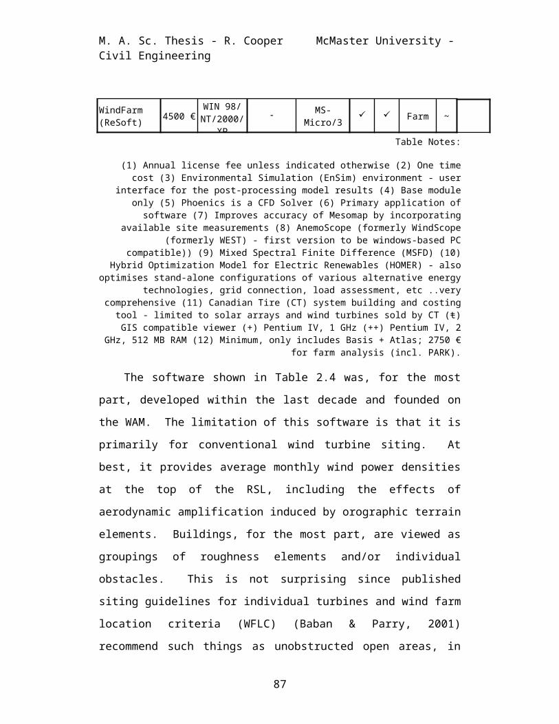
M. A. Sc. Thesis - R. Cooper McMaster University - Civil Engineering
WindFarm (ReSoft) 4500 €
WIN 98/NT/2000/
XP MS-
Micro/3 Farm ~
Table Notes:
(1) Annual license fee unless indicated otherwise (2) One timecost (3) Environmental Simulation (EnSim) environment - user
interface for the post-processing model results (4) Base moduleonly (5) Phoenics is a CFD Solver (6) Primary application ofsoftware (7) Improves accuracy of Mesomap by incorporating
available site measurements (8) AnemoScope (formerly WindScope(formerly WEST) - first version to be windows-based PC
compatible)) (9) Mixed Spectral Finite Difference (MSFD) (10)Hybrid Optimization Model for Electric Renewables (HOMER) - also
optimises stand-alone configurations of various alternative energytechnologies, grid connection, load assessment, etc ..very
comprehensive (11) Canadian Tire (CT) system building and costingtool - limited to solar arrays and wind turbines sold by CT (ŧ)GIS compatible viewer (+) Pentium IV, 1 GHz (++) Pentium IV, 2
GHz, 512 MB RAM (12) Minimum, only includes Basis + Atlas; 2750 €for farm analysis (incl. PARK).
The software shown in Table 2.4 was, for the most
part, developed within the last decade and founded on
the WAM. The limitation of this software is that it is
primarily for conventional wind turbine siting. At
best, it provides average monthly wind power densities
at the top of the RSL, including the effects of
aerodynamic amplification induced by orographic terrain
elements. Buildings, for the most part, are viewed as
groupings of roughness elements and/or individual
obstacles. This is not surprising since published
siting guidelines for individual turbines and wind farm
location criteria (WFLC) (Baban & Parry, 2001)
recommend such things as unobstructed open areas, in
87

M. A. Sc. Thesis - R. Cooper McMaster University - Civil Engineering
the path of prevailing winds, and preferably near the
crest of a hill or ridge (Canadian Wind Energy
Association, 2005). As models led to model
combinations, the development of commercial software is
prompting the evolution of integrated modelling
systems, which combine commercial software, specialised
microscale models, and GIS-functionality (e.g., WINDA
(Blennow & Sallnäs, 2004)).
In wind power meteorology, no attempt appears to
have been made to estimate the potential aerodynamic
amplification such obstacles may have on the flow;
amplification assessment seems to be limited to
orographic terrain and yet terrain terminology is being
carried over to the urban canopy (e.g., street canyon).
This research undertaking proposes that the
building-wind interaction produces aerodynamic
amplification that increases the wind speed in areas
within the UCL to at least levels experienced aloft.
Providing a way to estimate these winds would be of
great benefit to urban-scale WECS developers, urban
planners, architects, etc. To develop the theory
behind this concept, further understanding of the UCL
and the associated parameterisation schemes is
required.
88

M. A. Sc. Thesis - R. Cooper McMaster University - Civil Engineering
2.8 The Built Environment
In boundary layer modelling, the built or man-made
environment is represented by the UCL. Up to this
point, representation of the influence of an urban area
has generally been limited to its retardation effect on
the wind flow, as defined by the mean wind speed
profile and restricted in applicability to the region
above the UCL.
2.8.1 Urban Canopy Layer
The primary components within the urban canopy are
the buildings and the street canyons. Combined, these
components produce the urban form or morphology (i.e.,
the layout, density, shape, size, and orientation of
buildings and streets within the city). UCL modelling
simplifies the urban morphology by equating it to an
array of obstacles. Plate & Kiefer (2001) after
(Theurer, 1993) proposed that urban complexes could be
categorised into three basic patterns (i.e.,
homogeneous row, heterogeneous rectangular grid, and
real city block).
Wind resource assessment, for the most part, treats
urban terrain as a collection of roughness elements
(buildings) parameterised by roughness length [zo] and
an average height [zH]. These parameters are then used
89

M. A. Sc. Thesis - R. Cooper McMaster University - Civil Engineering
to estimate the wind speed velocity profile above the
UCL using wind speed measurements typically available
from meteorological stations within. At the
microscale, buildings are considered as obstacles,
which impede or significantly reduce the wind speed
(e.g., WAsP uses the dimensions, position, and porosity
of each obstacle to perform shelter modelling (Petersen
et al., 1998b)). This traditional approach fails to
reproduce the vertical structure of the flow
perturbations observed within an urban canopy (Cai,
2000), which is primarily governed by street canyon
energetics and dynamics (Rotach et al., 2005) (i.e.,
sensible heat flux [QH] (thermal) and turbulent kinetic
energy (TKE) (dynamic) (Martilli et al., 2002)). In
modelling the UCL, both horizontal and vertical
resolution must be increased. The use of higher-order
closure scheme CFD models is recommended (Dandou et
al., 2005) to account for mechanical turbulence
generated by airflow over and around buildings (Hanna &
Chang, 1992) and shadowing and street canyon radiation-
trapping (Hildebrand & Ackerman, 1984; Roulet, 2004).
The higher resolution and complexity in the UCL is
modelled using boundary layer wind tunnel (BLWT)
modelling (Plate, 1999; C. A. Miller & Davenport, 1998;
Maruyama & Ishizaki, 1988; Grant, Heisler, Gordon, &
90

M. A. Sc. Thesis - R. Cooper McMaster University - Civil Engineering
Herrington, 1988; Isyumov, 1978), computational fluid
dynamics (CFD) (Dayan, 2006), and mesoscale model-
imbedded urban parameterisation schemes (MacDonald,
2000; Martilli et al., 2002; Grosso, 1998). The
literature also includes research on enhancing existing
IBL (Landberg & Watson, 1994; Verkaik, 1999; Belcher et
al., 2003) and two-layer models (Clarke & Hess, 1974;
Verkaik, 1999; Verkaik, 2006) to more accurately
portray the urban RSL (MacDonald, 2000).
Research pertaining to UCL modelling and urban
parameterisation is being conducted in support of
erosion studies (Grant et al., 1988), air quality /
pollutant dispersion investigations (Fisher et al.,
2004; Rotach et al., 2005; Roulet, 2004; Christen,
Vogt, & Rotach, 2003; Berg, De Wekker, Shaw, Coulter, &
Allwine, 2004), pedestrian comfort and safety (Isyumov,
1978; Plate, 1999) and urban planning (Eliasson, 2000;
de Schiller & Evans, 1998; Bitan, 1992). This
literature can be broadly categorised as either
concerned with flow within and above the street
canyons, or with exchange processes between. A
comprehensive review of the last two years of
multidisciplinary and international urban climate
research has been compiled by Souch & Grimmond (2006).
91

M. A. Sc. Thesis - R. Cooper McMaster University - Civil Engineering
The challenge in modelling the UCL comes from the
need to average the mean and turbulent components of
velocity over both space and time, using RANS
equations, to evaluate the spatial and temporal
complexities of the flow field (Coceal & Belcher,
2005). The resulting momentum equations introduce new
terms that need to be parameterised. Of primary
significance is the parameterisation of elemental
canopy drag [Di] (Coceal & Belcher, 2005). Recent
urban-climate, scale-modelling developments have
focussed on turbulence, dispersion, and radiation
balance, and the need to compliment these findings with
both numerical and field observations. Findings from
both indoor and outdoor experiments indicate that
further research is required regarding the analysis of
thermally-stratified conditions and additional data
need to be provided for basic evaluation of the energy
balance (Kanda, 2006).
2.8.2 Urban Parameterisation Schemes
The theory behind UCL parameterisation (Souch &
Grimmond, 2006; Rotach et al., 2005) is founded on the
parameterisation of plant canopies (MacDonald, 2000;
Belcher et al., 2003; Coceal & Belcher, 2005; Cionco &
Ellefsen, 1998). Early studies on pesticide dispersion
92

M. A. Sc. Thesis - R. Cooper McMaster University - Civil Engineering
in crop fields laid the foundation for pollutant
dispersion studies within the UCL (Belcher et al.,
2003). Urban parameterisation schemes (e.g., the
porosity-drag approach (Dandou et al., 2005 after
(Piringer, 2002)) attempt to capture the significant
features of building and street canyon geometry using
appropriate scaling factors, or parameters, which
account for the thermal (Martilli, 2002) and mechanical
(Martilli et al., 2002) effects of the urban morphology
on the flow, within the fundamental conservation
equations. The primary scaling parameters applicable
within the UCL are the turbulence length [lc], the drag
length [Lc] or friction coefficient [] (MacDonald,
2000), and the horizontal adjustment distance length
scale or fetch [xo] (Coceal & Belcher, 2005).
Extensive research has been conducted defining and
developing these scaling parameters (Coceal & Belcher,
2005; Belcher et al., 2003) and mapping and/or
categorising urban morphology (Souch & Grimmond, 2006;
Fisher-Gewirtzman, Pinsly, Wagner, & Burt, 2005; C. A.
Miller & Davenport, 1998; Ellefsen, 1991; Grosso,
1998).
Related research is being conducted to define urban
terrain zones (Ellefsen, 1991) based on correlating
morphological values (e.g., plan area density (pad)
93

M. A. Sc. Thesis - R. Cooper McMaster University - Civil Engineering
[p] and frontal area density (fad) [f]) to land-use
classification. Application of LIDAR (Souch &
Grimmond, 2006) and GIS-assisted data-extraction from
DEMs (e.g., WINDA (Blennow & Sallnäs, 2004); Tanaka &
Moriyama, 2005; Bishop, 1998) have also been
investigated, as illustrated below.
Figure 2.23. Digital still video aerial imageryextraction techniques.
(a) A section of original image; (b) enhanced orthoimage; (c)digital surface model (DSM); (d) DSM minus digital terrain map(DTM); (e) classified shadows; (f) shack hypotheses; (g) ground
truth data (Bishop, 1998).
2.8.3 Mean Wind Speed Profile
The most important urban effects on the airflow are
summarised as follows:
94

M. A. Sc. Thesis - R. Cooper McMaster University - Civil Engineering
Pressure (form) drag, due to building walls; Friction (viscous) drag, due to street canyon
floors and roofs; Wake diffusion, due to the eddy structure within
turbulent wakes; Mean kinetic energy conversion into TKE in the
intense shear layer at the top of the UCL; and Heat flux modifications, due to shadowing,
radiation trapping, and building heat storage.(Roulet, 2004; Martilli et al., 2002; Roth, 2000)
The first four phenomena are mechanical processes,
while the last, which can lead to the generation of the
UHI effect, is due to thermal processes. Wake
diffusion entails both the mixing and diffusion of
momentum, heat, moisture, and pollutants.
Given the complex effects of urban morphology on
the flow within the UCL and the difficulties in
developing a unified parameterisation scheme, simple
estimations of the wind speed profile are obviously
problematic. In the literature, a simplified
exponential profile has been developed (MacDonald,
2000), which seems to be reserved for qualitative
comparisons vs. quantitative assessment of the actual
wind profile within the UCL (Coceal & Belcher, 2005).
Three-dimensional numerical modelling results
suggest that the urban canopy layer impacts both upwind
95
M. A. Sc. Thesis - R. Cooper McMaster University - Civil Engineering
and downwind flows (Belcher et al., 2003). The
disturbance, or IBL, is roughly the same as the mean
building height in a homogeneous canopy but can extend
to twice that height in heterogeneous canopies and/or
rough terrain (Grosso, 1998).
Ground level wind accelerations are caused by the
vertical pressure gradients that can be created by
taller buildings within the canopy (Coceal & Belcher,
2005) and building aerodynamics. Research attempting
to characterise street canyon flows suggests that three
flow regimes can develop (i.e., the isolated roughness
(f<0.13), wake interference ((0.13<f<0.25), and
skimming flow regimes (f>0.25) (Plate & Kiefer, 2001;
Xie, Huang, & Wang, 2006; MacDonald, 2000 after (Oke,
1992)). These are typified by turbulent, and/or
recirculating flow fields.
2.8.4 Building Aerodynamics
In the previous section urban parameterisation
schemes were discussed, which develop an estimate of
the mean wind speed profile within the UCL, using
scaling parameters based on the underlying urban
morphology. Homogenous zones within the heterogeneous
UCL were defined using key morphological values and
parameters, and the effect of transitioning between
96

M. A. Sc. Thesis - R. Cooper McMaster University - Civil Engineering
zones was explained as primarily governed by the fetch
of each zone.
Building aerodynamics research augments urban
parameterisation schemes by increasing the complexity
of the simplified cubic-array type representation of
the UCL, to include the effects of individual buildings
and their architectural details (e.g., roof shape).
The literature can be broadly categorised by angle of
flow incidence []. Orthogonal flow is seen as
producing Rankine vortex structures within street
canyons and horseshoe vortex structures in the wake of
buildings (Cook, 1985). Parallel flow can produce what
is generally referred to as channelling, (i.e., street
canyon and building geometry-induced flow amplification
similar to the orographic terrain induced speed-ups
previously discussed), while oblique or skewed flow is
characterised by complex vortex structures, including
delta-wind vortices (Zhang, Jiang, & Hu, 2006; Cook,
1990). The majority of the literature pertains to
orthogonal flow studies, including assessment of 2D vs.
3D modelling (Choi & Britter, 2004) and the influence
of roof configuration (Xie, Huang, & Wang, 2005).
Parallel and oblique flow studies range from simple
single canyon channelling (Skote, Sandberg, Westerberg,
Claesson, & Johansson, 2005) to complex networks of
97

M. A. Sc. Thesis - R. Cooper McMaster University - Civil Engineering
buildings and streets (P. J. Jones, Alexander, &
Burnett, 2004), including the effects of passages
through buildings (Blocken & Carmeliet, 2004),
interpreted as the venturi-effect (Bottema, 1999).
Field data collection to map out the complexities
of the flow field involving both temporal and spatial
variation is an onerous undertaking. The need to place
numerous instruments in various locations and heights
and difficulties in measuring direction result in
research in this field having to rely on a combination
of numerical methods and boundary layer wind tunnel
(BLWT) studies. Numerous studies have been conducted
comparing the results obtained using CFD models against
those produced in a BLWT (P. J. Jones et al., 2004;
Dalgliesh & Surry, 2003; Blocken & Carmeliet, 2004).
In BLWT studies point methods (e.g., hot-wire
anemometer or pressure sensor measurements), area
methods (Blocken & Carmeliet, 2004) (e.g. erosion or
scouring of a seeding material (P. J. Jones et al.,
2004)) and/or smoke visualisation (Blocken & Carmeliet,
2004; Guirguis, Hanna, Kotkata, & Gad, 1998) are used
to assess a scaled version of the generated flow field.
To apply BLWT results all of the significant processes
have to be scaled in a consistent fashion so that their
interaction reflects what would be observed in the real
98

M. A. Sc. Thesis - R. Cooper McMaster University - Civil Engineering
atmosphere (Xie et al., 2005). One of the main
challenges in using BLWT methods to study pollutant
dispersion and pedestrian comfort is that low wind
speeds are difficult to maintain (Choi & Britter, 2004;
Xie et al., 2005). The earliest BLWT building
aerodynamic studies were primarily interested in wind
loading, defined by pressure distributions, and dynamic
effects on the building structure. Pedestrian-level
wind studies did not begin until the late 1960s
(Blocken & Carmeliet, 2004).
Numerical methods primarily rely on CFD turbulence
models. These models can be classified as classical or
large eddy simulation (LES). The classical model is
based on RANS equations (e.g., the k– closure model),
which is by far the most used and validated (Zhang et
al., 2006). LES models (Cai, 2000) are based on the
subgrid scale (SGS) filtering model (Murakami, Ooka,
Mochida, Yoshida, & Sangjin, 1999), which is
computationally very demanding and mainly used in
research applications (Xie et al., 2005). At present,
there is some concern regarding the extent and location
of the wind amplification areas (P. J. Jones et al.,
2004) and turbulence structures, in general, generated
by CFD models (Zhang et al., 2006; Gratia, Reiter, & De
Herde, 2005), but results have been found to be
99

M. A. Sc. Thesis - R. Cooper McMaster University - Civil Engineering
sufficiently accurate in the presence of steady winds
(Riley, Gadgil, & Bazaroff, 1996). CFD, validated
through wind tunnel testing, is being applied in
dispersion or air quality studies (Zhang et al., 2006;
Xie et al., 2006; Xie et al., 2005), for pedestrian
comfort (C. Chang, 2006) and natural ventilation
(Gratia et al., 2005) assessments and urban planning
(Jun, 2005). These fields are actually at odds with
each other, since ideal conditions for pollutant
dispersion and natural ventilation often result in
pedestrian discomfort (Chan, So, & Samad, 2001).
Computational wind engineering (CWE), the application
of CFD in the field of wind engineering, is seen as a
relatively new undertaking (Murakami et al., 1999).
At the mesoscale, or perhaps even local level, the
orthogonal flow has been categorised into the following
three regimes: skimming flow (SF), isolated roughness
flow (IRF), and wake interference flow (WIF), as
illustrated below (Xie et al., 2006).
100

M. A. Sc. Thesis - R. Cooper McMaster University - Civil Engineering
Figure 2.24. Flow regimes within the UCL.The dashed-lines represent the wake development. As the streetcanyon width [W] is reduced, the flow regime (characterised by
wake development) transitions from isolated roughness flow (IRF)to wake interference flow (WIF) at W 3H, to finally produce theskimming flow (SF) regime at W 1.5H (Gratia et al., 2005 after
(Hussain & Lee, 1988)), where H is the representative buildingheight.
Given truly isolated buildings in an otherwise
homogeneous terrain (i.e., W > 50H (Sini, Anquetin, &
Mestayer, 1996)), the resulting flow regime is known as
fully independent wake flow (FIWF), wherein classic
vortex shedding occurs. This region does not typically
develop within an UCL due to plan area density. At the
other end of the scale where W <<1.5H, it becomes
evident that the effect of increased areal density has
a limit beyond which further increases have little
effect (Mfula, Kukadia, Griffiths, & Hall, 2005).
101

M. A. Sc. Thesis - R. Cooper McMaster University - Civil Engineering
A wake is the region of flow produced by a
perturbation (e.g., drag) characterised by unstructured
and/or structured turbulence commonly referred to as
eddies and vortices, respectively. van Bussel &
Mertens (2005) used CFD to validate the empirical
equation for the semi-elliptical wake zone proposed by
Wilson (1979). Bottema (1999) used the geometric
influence scale parameter [Lg] (Cook, 1990) to
establish frontal (1Lg) and leeward (4Lg) wake region
lengths (Bottema, 1993) to develop a 2D representation
of the wake region. It is within a relatively small
region of the wake, seen in 3D as having a similar
horizontal profile at the vertical edges of buildings
to that produced vertically at horizontal edges, that
flow amplification is observed (van Bussel & Mertens,
2005). Defining the thresh-hold aspect ratios of each
flow regime is crucial to the development of a
comprehensive description of the flow above, and the
recirculation structures within, street canyons. The
parameters of interest are the geometric aspect ratios,
primarily the street, canyon, or side aspect ratio
(sar) [W/H] and the frontal aspect ratio (far) [L/H],
where L is the length of the canyon normal to the wind
direction. Variation in how these aspect ratios are
defined makes it difficult to compare study findings.
102

M. A. Sc. Thesis - R. Cooper McMaster University - Civil Engineering
Wind tunnel model aspect ratios based on street canyon
geometry (Sini et al., 1996) produce opposite far and
sar definitions from those based on building geometry
(Hussain & Lee, 1980). Other studies create additional
confusion by defining the reciprocals of these ratios
(e.g., H/W (Xie et al., 2006)).
At the microscale within each of the flow regimes,
further stratification has been defined based on the
street canyon vortex structure, as illustrated in
Figure 2.25. Vortex structure categorisation pertains
to orthogonal flow and is primarily based on direction
of rotation and number of vortices within a given
street canyon.
(a) Vortex Structure I(a)
(b) Vortex Structure I (b)
103

M. A. Sc. Thesis - R. Cooper McMaster University - Civil Engineering
(c) Vortex Structure II
(d) Vortex Structure III
Figure 2.25. Vortex structure categorisation.The associated canyon and building aspect ratios are (a) W/H1=0.29& H1/H2=1 (b) W/H1 = 0.5 & H1/H2 = 1 (c) W/H1 = 1.11 & H1/H2 = 0.9
(d) W/H1 = 5.88 & H1/H2 = 1 (Xie et al., 2006)
Additional research involving buildings of varying
heights has explored the implications of cross-canyon
building height aspect ratio (Xie et al., 2006) or
relative height ratio [H1/H2] (Chan et al., 2001) on
vortex structure development as illustrated, where H1
and H2 are the upwind and downwind building heights,
respectively.
104

M. A. Sc. Thesis - R. Cooper McMaster University - Civil Engineering
Figure 2.26. Effect of varying building height oncanyon vortex structure.
The proportion of four buildings is figured to the left of eachconfiguration (Xie et al., 2005 p. 4527)
Detailed investigation of canyon vortex structures
has been conducted through LES, highlighting the
influence of flow direction (Zhang, Weimei Jiang, &
Miao, 2006), secondary flows (Macfarlane & Joubert,
1998), and roof configuration (Souch & Grimmond, 2006)
(Figure 2.27). Louka, Belcher, & Harrison (2000)
suggest that structured vortices are actually very
short lived and weaker than unsteady turbulent
105

M. A. Sc. Thesis - R. Cooper McMaster University - Civil Engineering
fluctuations due to the unsteady position of the shear
layer. Worthy of further exploration are the
inherently higher wind speeds at the radius of the
forced-vortex core of these vortices. It is suggested
that most of the vortices experienced in the field of
wind engineering can be represented by the Rankine
vortex, within which the core is surrounded by a free-
vortex outer region (Cook, 1985). There is very little
in the literature regarding delta-wing vortex
development, as it pertains to skewed flow angles whose
investigation is under-represented.
106

M. A. Sc. Thesis - R. Cooper McMaster University - Civil Engineering
Figure 2.27. Effect of roof configuration on canyonvortex structure.
(Xie et al., 2005 p. 4523)
Figure 2.28 below, summarises the cross-canyon wind
speed variation as observed in each of the numbered
configurations illustrated above.(a) Configuration 1 through 4 (b) Configuration 1, and 5
through 7
107

M. A. Sc. Thesis - R. Cooper McMaster University - Civil Engineering
Figure 2.28. Cross-canyon horizontal mean wind speedvariation.
Situations relate to the configurations illustrated in Figure2.27. Dimensionless cross-canyon distance [X/B], where B is the
canyon width and X is the cross-canyon horizontal distance.Negative velocities correspond to clockwise rotating vortices at
street-level. Extracted from Xie et al. (2005) p. 4525.
The literature pertaining to oblique flow studies
primarily focuses on architectural details (Jamieson,
Carpenter, & Cenek, 1992) (e.g., pilotis or support
columns, passages (Isyumov. & Davenport, 1977), and
setbacks (Yamamura & Kondo, 1993)) and street canyon-
induced wind amplification (P. J. Jones et al., 2004;
Bottema, 1999). The majority pertains to the effect of
the presence of a tall building on pedestrian-level
winds (Yamamura & Kondo, 1993). Explicit formulation
of wind amplification in terms of aspect ratios is
difficult due to complexities and non-linearities. For
the most part, oblique flow research has produced more
qualitative than quantitative findings. These findings
108
M. A. Sc. Thesis - R. Cooper McMaster University - Civil Engineering
categorise various effects by architectural detail
(e.g., venturi, gap, channel, tower, and shelter
effects (Gandemer, 1977)), provide illustrative plots
based on aspect ratios (Chan et al., 2001), and/or
suggest general rules of thumb (Bottema, 1999).
In the field of wind engineering, concerned with
wind loading on structures, decades worth of BLWT study
findings have been summarised in the form of non-
dimensional pressure coefficient tables (Canadian
Commission on Building and Fire Codes, 2005). These
pressure coefficients are dependent on the flow regime
(i.e., mean wind speed and angle of incidence), UCL
parameters, and the geometrical aspect ratios of the
built environment (Gratia et al., 2005; Canadian
Commission on Building and Fire Codes, 2006). In
Canada, these data are published in the National
Building Code (NBC), along with recommended correction
factors intended to assist designers in calculating
mean pressures and forces on built structures and their
components for safety and durability considerations.
The wealth of data available from this field has
only recently been tapped by other fields (e.g.,
natural ventilation (Hussain & Lee, 1980) and
contaminant infiltration (Riley et al., 1996)).
109

M. A. Sc. Thesis - R. Cooper McMaster University - Civil Engineering
Literature on the use of pressure coefficients to
determine local wind velocities, includes correlating
surface pressure fields to the flow regime (Hussain &
Lee, 1980) and Grosso's (1992) parametric pressure
distribution model. The field of wind power
meteorology should further explore the applicability of
these data in the determination of wind amplification
zones in support of truly urban-scale BAWTs.
Under closer scrutiny, there is some concern
regarding the transferability of these pressure
coefficients. One of the primary challenges is that
the intended reference (or design) wind speed used in
calculating the pressure and/or force on the structure
and/or its elements, is a statistically derived maximum
gust. Other challenges are presented through the
various correction factors. Hanzlik, Diniz, Grazini,
Grigoriu, & Simiu (2005) question the neglect of the
influence of building orientation within ASCE 7
'Minimum Design Loads for Buildings and Other
Structures', published by the American Society of Civil
Engineers (ASCE) and referenced by the International
Building Code (IBC), published by the International
Code Council (ICC). Correction factors, in general,
are applied only to a design wind speed while the
pressure coefficients used to calculate the wind-
110

M. A. Sc. Thesis - R. Cooper McMaster University - Civil Engineering
induced pressures and forces remain based on the
results of tests on isolated bodies under specific BLWT
flow conditions (Hussain & Lee, 1980). Based on this
neglect of the influence of neighbouring structures,
Plate & Kiefer (2001) state that standard wind tunnel
results cannot be used in the assessment of urban
areas. The reader is referred to Plate & Kiefer’s
(2001) article for an excellently illustrated and
explained summary of building code correction factors
and BLWT conditions in boundary layer meteorology
terms.
Similar to the notion of codifying diffusion
processes presented by Plate & Kiefer (2001) and the
already codified wind forces/pressures, this research
undertaking proposes the need for codification of
building-induced flow amplification. Most studies are
concerned with forces and pressures, the velocity
field, or the pollutant concentration field, and not
with the relation of the three to each other within the
UCL. More specifically, there appears to be very
little literature pertaining to a correlation between
forces or pressures and mean wind velocities.
In wind power meteorology input, analysis, and
storage of wind, land-use, and urban parameterisation
111

M. A. Sc. Thesis - R. Cooper McMaster University - Civil Engineering
data suggest that a structured data management and
decision support system would be beneficial. As such,
a review of literature pertaining to various systems
currently used in support of renewable energy
assessment was conducted.
2.9 Decision Support Systems
In the literature, a computer-based structured
presentation of a combination of analytical tools
accessing pertinent data in support of making a
decision is generally called a decision support system
(DSS). At the heart of every DSS is the ability to
collect, analyse, and report in a fashion conducive to
making a decision regarding the matter at hand, as
illustrated below for the Wind Load Design Environment
(WiLDE) application.
112
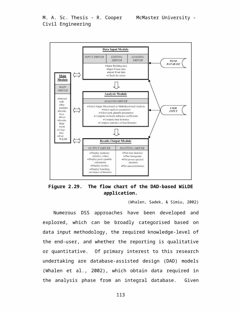
M. A. Sc. Thesis - R. Cooper McMaster University - Civil Engineering
Figure 2.29. The flow chart of the DAD-based WiLDEapplication.
(Whalen, Sadek, & Simiu, 2002)
Numerous DSS approaches have been developed and
explored, which can be broadly categorised based on
data input methodology, the required knowledge-level of
the end-user, and whether the reporting is qualitative
or quantitative. Of primary interest to this research
undertaking are database-assisted design (DAD) models
(Whalen et al., 2002), which obtain data required in
the analysis phase from an integral database. Given
113

M. A. Sc. Thesis - R. Cooper McMaster University - Civil Engineering
the multi-criteria analysis required in this
undertaking, expert systems, based on rules of thumb
and guidelines (Kaminaris, Tsoutsos, Agoris, & Machias,
2006), were also explored. These are often coupled
with qualitative modelling using fuzzy-logic (Rylatt,
Gadsden, & Lomas, 2001), which is seen as justified in
analysis involving high levels of uncertainty (Germano
& Roulet, 2006, after (Paelinck, 1978).
The majority of the DSSs involving assessment of
the interaction between the built environment and
climatological processes have been developed in support
of sustainable urban planning and development (Tweed &
Jones, 2000). Primarily qualitative in nature,
planning support systems (PSSs) (Bishop, 1998), spatial
decision support systems (SDSSs) (Ramachandra, Krishna,
& Shruthi, 2004), and urban planning simulations and
decision support technologies (O’Looney, 2001) produce
guidelines and rules of thumb (de Schiller & Evans,
1998). In the field of passive and low energy
architecture (PLEA), encompassing bioclimatic design
principles and green building design optimization
algorithms (Wang, Rivard, & Zmeureanu, 2005), pre-
design guidelines for passive solar architecture (Rabah
& Mito, 2003) and the concept of an energy and
environmental prediction (EEP) model (Tweed & Jones,
114

M. A. Sc. Thesis - R. Cooper McMaster University - Civil Engineering
2000) have been developed. In the field of wind
engineering the Wind Load Design Environment for Low-
Rise Structures (WiLDE-LRS) has been developed to
provide design guidance by improving on the empirical
nature of the data presented in the building codes
(Whalen et al., 2002).
Energy planning (EP) DSSs focus on the impact of
urban planning concepts on renewable energy potential
(e.g., solar energy planning (SEP) (Rylatt et al.,
2001; Ramachandra, 2006) and biomass energy potential
assessment (BEPA) (Ramachandra et al., 2004)).
Renewable energy source (RES) DSSs (Bishop, 1998) in
support of EP are generally concerned with defining the
technological potential (i.e., the performance of the
renewable energy extraction device) based on the
theoretical climatic potential subject to socio-
economic restraints (Voivontas, Assimacopoulos,
Mourelatos, & Corominas, 1998). With the advent of
commercially available software, existing DSSs
specifically in support of wind energy assessment have,
for the most part, focused on high-level socio-economic
aspects. These assessments involve determination of
the financial and legal aspects of connecting wind
farms to the electrical grid (Kaminaris et al., 2006)
115
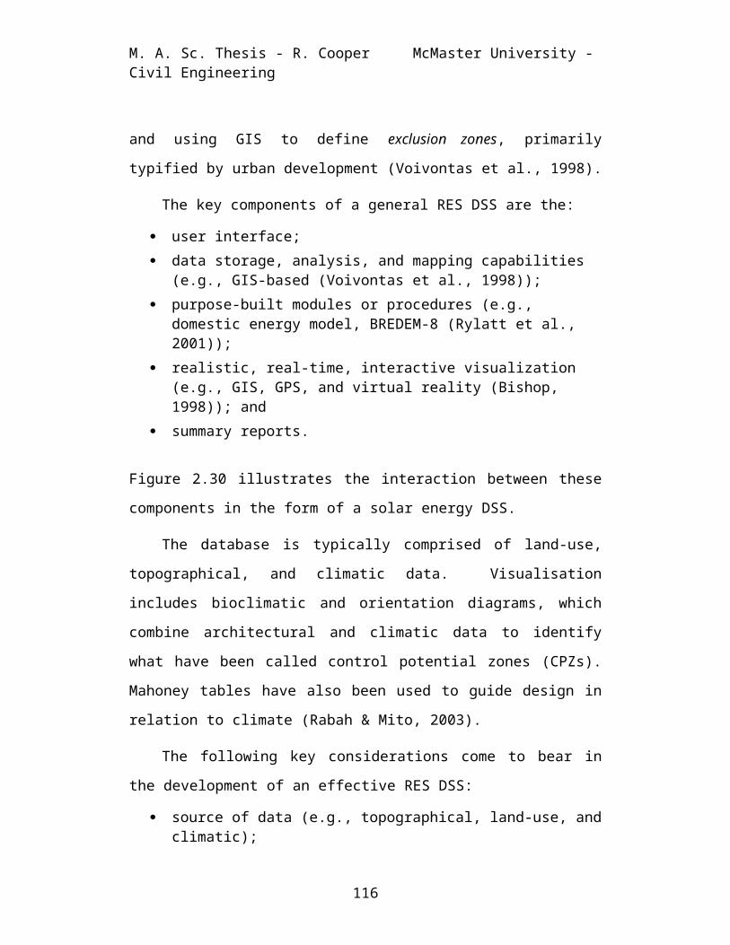
M. A. Sc. Thesis - R. Cooper McMaster University - Civil Engineering
and using GIS to define exclusion zones, primarily
typified by urban development (Voivontas et al., 1998).
The key components of a general RES DSS are the:
user interface; data storage, analysis, and mapping capabilities
(e.g., GIS-based (Voivontas et al., 1998)); purpose-built modules or procedures (e.g.,
domestic energy model, BREDEM-8 (Rylatt et al., 2001));
realistic, real-time, interactive visualization (e.g., GIS, GPS, and virtual reality (Bishop, 1998)); and
summary reports.
Figure 2.30 illustrates the interaction between these
components in the form of a solar energy DSS.
The database is typically comprised of land-use,
topographical, and climatic data. Visualisation
includes bioclimatic and orientation diagrams, which
combine architectural and climatic data to identify
what have been called control potential zones (CPZs).
Mahoney tables have also been used to guide design in
relation to climate (Rabah & Mito, 2003).
The following key considerations come to bear in
the development of an effective RES DSS:
source of data (e.g., topographical, land-use, andclimatic);
116

M. A. Sc. Thesis - R. Cooper McMaster University - Civil Engineering
data collection methodology (e.g., database-assisted and/or user-input);
level of required technical expertise; integration of analysis modules; adaptability and re-use of algorithms (Wang et
al., 2005); accessibility & effort-level vs. accuracy; and ease of use.
117
M. A. Sc. Thesis - R. Cooper McMaster University - Civil Engineering
Figure 2.30. Solar energy decision support system.(Ramachandra, 2006)
Task-specific DSSs are being advocated as opposed
to the creation of an all-encompassing, monolithic
system (Bishop, 1998), which may be impossible to
implement and/or yield difficult to interpret results
(Tweed & Jones, 2000). In design, which is primarily
an iterative undertaking, simplicity of input,
processing, and output are vital (Whalen et al., 2002).
2.10Literature Review Summary
This literature review has attempted to organise
the wealth of transferable, interdisciplinary knowledge
in support of the development of an urban-scale RES
DSS. Given that wind power meteorology is a relatively
new field, solutions to perceived limitations
conceivably reside in related disciplines. Though
plagued by inconsistencies, areas of outright dispute,
and serious limitations regarding a quantitative
parameterised assessment of building-induced wind
amplification, there is sufficient material within the
published literature to conceptualise a stratified
approach to the assessment of urban-scale wind energy
potential.
118

M. A. Sc. Thesis - R. Cooper McMaster University - Civil Engineering
An astounding amount of transferable research has
already been conducted in other fields. As an
interesting example, acid rain studies are producing
the urban terrain characterisation-zone maps required
by UCL modellers (Ellefsen, 1991). In the wake of a
growing awareness regarding the impact on human
comfort, air quality, and energy consumption (Eliasson,
2000) that urban architecture can have, there is a
movement underfoot to bridge the gap between scientific
understanding of climatic processes and the associated
impact of design practices (Wisse, 1988). A myriad of
available software, the relatively recent refocus on
bioclimatic design, and the green building movement all
support the need for DSSs linking urban planning,
architectural detail, and their associated climatic
implications. The prevalence of such systems in
support of urban-scale solar energy planning (SEP)
calls for augmentation by an associated urban-scale
wind energy planning (WEP) DSS, given the intrinsic
connection between solar and wind energy potential.
The primary challenge in this research undertaking
will be to assimilate what has been accomplished to
date in the field of wind power meteorology and augment
it with a more detailed appraisal of building-induced
acceleration zones. The uncertainties involving key
119

M. A. Sc. Thesis - R. Cooper McMaster University - Civil Engineering
parameters (e.g., roughness length), wind speed
profiles, and pressure coefficients (potentially
providing a summarisation of building-induced wind
amplification) will need to be resolved, in order to
develop a comprehensive assessment of these wind energy
potential micro-zones. Land-use data, especially
details pertaining to building height, will need to be
gathered and/or generated. It is primarily the
stratified, multi-disciplinary approach to wind field
assessment, within the existing literature, that is
providing the greatest challenge. For example, at the
microscale, drag-based effective roughness length is
not correlated to mesoscale roughness maps. A
generalised approach will need to be developed to
generate the pertinent variables based on available
land-use data to calculate the parameters necessary to
estimate the wind speed profiles. For the most part,
wind speed profile equations and probability
distributions, require an iterative approach to solve
and fit, respectively. Careful consideration of
accuracy vs. simplicity and ease of use will be
required in the development of the proposed DSS.
Given the focus of recent research on validating
numerical models based on empirical and theoretical
equations, one must delve back over a decade to gain a
120

M. A. Sc. Thesis - R. Cooper McMaster University - Civil Engineering
better understanding of the underlying transferable
scientific principles. In general, the literature is
severely lacking with regard to structure-induced wind
amplification, primarily focussing on orthogonal flow-
induced canyon vortex structures. Finally, there is
some concern regarding the compounding of inaccuracies
(i.e., using a probability distribution function
estimation of the mean wind speed to develop the mean
wind speed profile using a logarithmic profile, which
is then used as the reference velocity for building-
induced amplification assessment). Careful
consideration of unavoidable inaccuracies will be
required to calculate appropriate tolerance bands for
the amplified mean wind speed and wind power density
estimates.
The development of a conceptual model for urban
wind energy planning (UWEP) will be discussed in the
following chapter. This conceptual model develops the
methodology upon which the proposed prototype UWEP DSS
is based.
121

M. A. Sc. Thesis - R. Cooper McMaster University - Civil Engineering
3 CONCEPTUAL MODEL DEVELOPMENT
The building industry has made considerable
progress in evaluating the energy and environmental
implications of resource deployment in building
construction using assessment tools such as the
Building Research Establishment's Environmental
Assessment Method (BREEAM) and ECD Energy & Environment
Canada Ltd.'s Green Globes. Numerous guidelines (e.g.,
Leadership in Energy and Environmental Design (LEED)
and R2000/EnerGuide) have been developed to direct
practitioners in the investigation of life-cycle costs
associated with building material and construction
methodology selection. Simulation tools such as the
Sustainable Buildings Industry Council's Energy-10, the
Californian Energy Design Resources program's QUick
Energy Simulation Tool (eQuest), and the Department of
Energy's DOE-2 have been developed, through which the
energy efficiency of the latest building technologies
can be comparatively assessed.
Industry must now move beyond the current
guidelines, which focus primarily on energy efficiency,
to a consideration of how to make a structure self-
sufficient through its ability to produce the energy
its occupants will inevitably consume. An urban
122

M. A. Sc. Thesis - R. Cooper McMaster University - Civil Engineering
renewable energy source (URES) assessment tool would
help achieve this objective. The photovoltaics
algorithm, recently developed for DOE-2.2 suggests that
industry is heading in this direction (Hirsch, 2006).
Unfortunately, the only consideration that wind is
given within existing building energy simulation tools
is with regard to its role in natural ventilation and
the impact of infiltration on building heating and
cooling costs. This research undertaking takes steps
towards future assessment of wind as an energy source
within building energy simulation tools.
3.1 Urban Renewable Energy Source Assessment
The inherent opportunities to maximise renewable
energy (RE) from various sources (e.g., sun, wind,
ground heat, etc.) depend on the urban morphology
(e.g., plan orientation, placement of structures within
the plan, and the architectural detail of the
individual structures) and the meteorological-
morphological interactions (Grosso, 1998). URES
assessment would primarily differ from classic RES
assessment by including an analysis of the interaction
between pertinent meteorological processes and the
underlying morphology. Such an assessment could
support iterative evaluation of building configuration
123

M. A. Sc. Thesis - R. Cooper McMaster University - Civil Engineering
implications on potentially extractable renewable
energy. One possible configuration of a modular URES
DSS is portrayed in Figure 3.1.
DECISION M AKER URES-DSSDATABASESANALYSIS M O DULES
SOCIO -ECO NO M IC M O DULELife-cycle analysis
Energy Policy M akersLegal fram ework & financial incentives
RES ASSESSM ENT M O DULE(e.g. hydro, biom ass, geotherm al, solar, wind, etc.)
Theoretical PotentialBased on m eteorological, hydrological, geological, etc. data.
RES DataG eographicalM eteorological ArchiveW ind Atlasetc.
Available Potential
Influence of local terrain, land-use, built environm ent m orphology, etc.
G eophysical DataTopographicalLand-useRoad ClassificationBldg Classification
Technological Potential
Portion of available energy that can be extracted by the energy conversion device.
Technical DataPerform ance characteristicsSystem efficiencies
ENERG Y CO M PUTATIO N
M O DULE
Energy Dem and Data(including conservation m easures)Forecasting Data
Econom ic DataConstruction costs M aintenance costs DepreciationInflationProject life span
Select a SIte
Can sufficient energy be produced?
Are there negative socio-
econom ic im plications?
Can they be
overcom e or
m itigated?
Yes
LO CAL AUTHO RITIES
UTILITIESon vs. off grid
INVESTO RS
No
Yes
Yes
Viable Project
No
1
2
ENVIRO NM ENTAL IM PACT M O DULE
SO CIO -ECO NO M IC CO ST
No
Figure 3.1. Urban Renewable Energy Source (URES) DSS.Based on Ramachandra (2006) and Voivontas et al. (1998). The
shaded areas highlight areas of focus of the proposed WEP module.
The URES module algorithms would be structured in such
a way as to accommodate the assessment of a variety of
RES for a given location. Modularisation of the
analysis algorithms and integral databases would
produce an extremely versatile framework. It is
124

M. A. Sc. Thesis - R. Cooper McMaster University - Civil Engineering
through the inclusion of detailed morphological data,
parameterised using road and building classification
schemes, that calculations of available potential energy can
truly reflect urban-scale influences (e.g., street-
canyon radiation trapping, shadowing, and building
aerodynamics-induced wind-amplification).
Since there are several solar energy planning (SEP)
DSSs already in existence (Ramachandra, 2006; Rylatt et
al., 2001) and the other RES currently have limited
applicability in an urban setting, the body of this
research will focus on the development of an urban wind
energy planning (UWEP) module. The UWEP module would
fit into a complete URES DSS as illustrated by the
shaded regions within Figure 3.1. Studies have shown
that traditional wind turbine siting guidelines may
result in the selection of suboptimal heights and
locations (Campbell & Stankovic, 2001b). An assessment
of the potentially amplified wind speed in the
neighbourhood of urban morphological features could
have a profound effect on both the design of wind
energy extraction devices and their siting. The body
of this research introduces the concept of urban wind
as a manipulable resource, drawing on theory from
several different fields. Concepts long understood in
the field of meteorology and geography, such as tunnel
125

M. A. Sc. Thesis - R. Cooper McMaster University - Civil Engineering
and hill effects, will be brought to bear in the
assessment of the wind resource within the urban canopy
layer (UCL). Research findings and theory from the
field of building aerodynamics will be used to quantify
building-induced wind amplification phenomena.
The concept of urban-scale building integrated
and/or mounted wind turbines (BUWT) is still in its
infancy. There are only a small number of
manufacturers currently exploring the development of
urban wind energy conversion systems (Campbell &
Stankovic, 2001b). The underlying premise is that if
the configuration of structures on a site, and/or
individual features of a structure, can accelerate the
air flow through the energy extraction device, smaller
urban-scale machines could conceivably become
economically viable. Since these designs are still at
the patent-pending stage, performance characteristics
required to determine how much energy could be
extracted given particular wind conditions are not yet
available. As such, the proposed DSS will focus on
quantifying the energy potentially available for
extraction, leaving the assessment of the socio-
economic feasibility of urban-scale electrical energy
production (Celik, 2003) to other software applications
(e.g., HOMER and RETScreen). A preliminary study of
126

M. A. Sc. Thesis - R. Cooper McMaster University - Civil Engineering
the socio-economic considerations pertaining to wind
turbines in a built environment can be found in Cace et
al.’s (2007) report.
3.2 Scope of Applicability
The planning tool is intended for use by a broad
spectrum of individuals, including, but not limited to
homeowners, engineers, architects, and developers. The
tool would be applicable to both new and existing urban
developments. To facilitate UWEP at an existing site,
and/or in the early stages of urban development, the
proposed tool would need to be flexible, interactive,
and able to extract data from, and provide data to, a
suitable design platform (e.g., AutoCad). For existing
sites, ideally, the site plan would be uploaded into
the assessment tool, to allow for topographical,
geographical, and meteorological detail to be
superimposed. For new developments the superimposed
detail, in conjunction with a predefined optimal plan
and architectural feature configuration, would form the
initial layout. The proposed planning tool, as
conceptualised in Figure 3.2, would incorporate a
database-assisted design (DAD)-type approach and
encompass the shaded portions of the RES assessment
module in Figure 3.1.
127

M. A. Sc. Thesis - R. Cooper McMaster University - Civil Engineering
3.3 Configuration of the Conceptual Model
The platform of the proposed UWEP DSS, illustrated
below, will be based on Microsoft Excel, due to the
various calculations that will be required throughout
the assessment, the need to build databases and store
data, and the desire to accommodate as many future
users as possible. Visual Basic for Applications
(VBA)-based forms will provide the user-interface for
data input, internal database-data extraction, and the
capability to populate fields within the module's
worksheets, wherein the calculations are performed.
This will simplify the exchange of data and protect the
integrity of both the integral database and the
analysis worksheets.
128

M. A. Sc. Thesis - R. Cooper McMaster University - Civil Engineering
DATA INPUT O UTPUT
USER INTERFACE
UW EP M ODULE
EXTERNAL DATABASE
Sum m ary Reporte.g. site and building configuration, am plification zones, estim ated wind energy, peak energy m onths, and recom m endations.
INTERNAL DATABASE
Site Characteristicse.g. location, orientation, land-use category, building and road classification.
Building Characteristicse.g. orientation, height, width, depth, roof type, and pitch.
M eteorological Datae.g. hourly wind speed and direction.
Figure 3.2. Conceptual Model of the UWEP DSS.
Data will primarily be obtained from external internet-
based databases and applications, while parameters
required for mathematical computations will be
extracted from an internal database. The required data
can be categorised as:
Meteorological (e.g., wind speed and direction), Geographical (i.e., latitude and longitude co-
ordinates), Topographical (e.g., land-use and urban
subregion), and Morphological, (e.g., street widths and building
configurations).
129

M. A. Sc. Thesis - R. Cooper McMaster University - Civil Engineering
Meteorological data would be obtained from an internet-
based wind atlas (e.g., the Ontario Wind Resource Atlas
and the Canadian Wind Energy Atlas) or generated from
the time series data (TSD) of a nearby meteorological
station, provided by Environment Canada's internet-
based National Climate Data and Information Archive.
Co-ordinate data would be obtained from an online
database (e.g., Geo-coder). Topographical and
morphological data would be input by the user through
selection of predefined options within an associated
VBA form. The user would be directed to a national-
level, geographical society and/or government regulated
website (e.g., Natural Resources Canada (NRCan) (2006)
Atlas of Canada) to identify land-use categories and
satellite image applications (e.g., MapQuest and
Google Maps) to identify the representative urban
subregion. To limit the scope of this research
undertaking, it is proposed that orographic terrain
(e.g., mountains and hills) feature-induced effects be
assessed by an add-on submodule through future
development of the proposed UWEP DSS. The reader is
directed to the literature of Jacobson & Malte (2005),
Troen & Petersen (1989), and Verkaik (1999) for details
130

M. A. Sc. Thesis - R. Cooper McMaster University - Civil Engineering
regarding the underlying methodology of such an
undertaking.
The UWEP module will be comprised of various
submodules to manipulate the wind speed and direction
data, assess wind amplification, identify the location
and size of the amplification zones, and calculate the
wind energy available for extraction. The UWEP
submodules would extract the appropriate parameters
required in the calculations from specialised tables of
an internal database based on user input. This
internal database will minimise the level of expertise
and user-effort required to parameterise the urban
morphology and building aerodynamics-induced wind
amplification. It would be comprised of the following
tables:
latitude and longitude co-ordinates (for select cities),
roughness parameters (based on land-use categorisation),
urban parameters (based on road and building type classification), and
wind speed amplification factors.
The results of the assessment will be presented in
a summary report, generated from the data, calculated
values, and associated graphs stored in the analysis
131

M. A. Sc. Thesis - R. Cooper McMaster University - Civil Engineering
worksheets. The primary outputs of the proposed tool
will be:
Project details summary (e.g., name, address, comments, etc.)
Morphological (e.g., urban subregion) Subject building dimensions and features (e.g.,
roof type and pitch) Amplification zone areas by building face Wind power density by zone Wind energy by building face Windy season months
Graphical representations will be comprised of user-
saved images and graphs generated by the proposed tool.
The summary report would include recommendations
concerning building orientation and architectural
feature characteristic (i.e., roof type and pitch)
changes. These recommendations could potentially
enhance wind amplification, which in turn would yield
higher levels of wind energy available for extraction.
The proposed methodology of wind energy assessment,
including the meteorological-morphological interactions
resulting in wind amplification, will now be discussed.
3.4 Wind Energy Assessment Methodology
Wind energy assessment requires estimation of
temporally and spatially variable wind statistics. The
132

M. A. Sc. Thesis - R. Cooper McMaster University - Civil Engineering
proposed tool would accommodate both vertical and
horizontal spatial variation by defining the following
scales:
Region, City (mesoscale), Neighbourhood (local scale), and Site (microscale).
The horizontal spatial variation is only considered at
the microscale. Correspondingly, the tool would
perform the following tasks in developing the wind
statistics:
Estimate the regional wind statistics, Develop the mesoscale wind speed profile, Determine the local scale wind amplification, and Calculate the building aerodynamics-induced
microscale wind amplification.
Performance of these tasks involves meteorological and
morphological considerations, which will now be
discussed in turn.
3.4.1 Meteorological Considerations
The first task performed by the UWEP module would
be to assess the spatial and temporal variation of the
wind at the site. Spatial variation is represented by
the mean wind speed profile [ ], as illustrated in
133

M. A. Sc. Thesis - R. Cooper McMaster University - Civil Engineering
Figure 3.3. The UWEP module will calculate the mean
wind speed profile based on the regional wind
statistics. It will consider the mean annual, regional
wind statistics provided by the wind atlases as the
mesoscale wind. The mesoscale wind is considered to
prevail above the surface layer (SL) and remain
relatively constant over several kilometres.z
Urban Boundary LayerSurface Layer
G eostrophic W ind
M esoscale W ind
W ind Direction
)z(u
Figure 3.3. The vertical stratification of the urbanboundary layer.
In regions where there are distinct seasons, a
seasonal assessment would be conducted using time
series data (TSD). The TSD will be used to calculate
the mesoscale wind statistics unless the meteorological
station is greater than five kilometres from the site
in which case the geostrophic wind statistics will be
calculated. The geostrophic wind prevails above the
urban boundary layer (UBL) and remains relatively
constant over distances greater than five kilometres.
In these regions a hybrid solar-wind energy extraction
134

M. A. Sc. Thesis - R. Cooper McMaster University - Civil Engineering
system should be considered (Eke, Kara, & Ulgen, 2005),
given that the wind resource is typically plentiful
during periods when solar energy is less plentiful and
vice versa.
Temporal variation is defined by the regional wind
statistics in the form of a wind speed histogram
(Figure 3.4 (a)) and/or probability distribution and an
associated wind direction rose (Figure 3.4 (b)). Wind
direction is of primary importance when considering
fixed-direction, wind energy extraction devices. Given
that very few sites are truly subjected to uni-
directional winds, with most actually experiencing
omni-directional winds, the data are best presented in
the form of a wind direction rose. By grouping
cardinal sectors by quadrant, two to three dominant
wind directions can often be identified for most sites.
For example, in Figure 3.4 (b) the dominant directions
could be summarised as SSW (combining WSW, SSW, and S),
SE (SSE and ESE), and N. The assessment tool would
primarily rely on the two most dominant directions, to
be referred to as the primary and secondary wind
directions, to determine the presence and type of
aerodynamic effect likely to result in wind
amplification.
135

M. A. Sc. Thesis - R. Cooper McMaster University - Civil Engineering
(a) Wind Speed Histogram (b) Wind Direction Rose
Figure 3.4. Wind speed histogram (a) and directionrose (b).
Having fully defined the wind climate, the UWEP module
would proceed on to the assessment of wind
amplification involving morphological considerations at
both the local and microscale.
3.4.2 Morphological Considerations
The literature concerning the implications of
building aerodynamics on the flow field indicates that
wind amplification is governed by the morphological
parameters of the underlying terrain on several scales
and dependent on the associated flow regime. Though
there is a general awareness of wind amplification,
including folklore pertaining to windy street corners
and/or intersections, the underlying sentiment is best
136

M. A. Sc. Thesis - R. Cooper McMaster University - Civil Engineering
summarised by “wind patterns in complex terrain … are
so complicated that they defy analysis or accurate
description” (H. Liu, 1991 p. 62). The underlying
premise of this body of research is that local scale
and microscale amplification can be estimated using
published comfort parameters and pressure coefficients,
respectively. Wind amplification exceeding a factor of
2 has been recorded (H. Liu, 1991) resulting in a
potential 8X wind power increase. Amplification up to
a factor of 3 has been predicted by CFD analysis of an
urban area (Gandemer, 1977), corresponding to a
potential 27X wind power increase. Determination of
the magnitude and location of amplified wind speed
zones within an urban setting may prove that urban wind
energy extraction is a viable undertaking.
Studies involving the influence of building
configurations on ground-level wind speeds have
developed the concept of a comfort parameter as a
function of turbulence intensity and wind amplification
(Gandemer, 1977), dependent on the morphological
configuration at a local scale. The proposed tool
would correlate the urban subregion morphology to
comfort parameter-based amplification factors for
various aerodynamic effects, within an internal
137

M. A. Sc. Thesis - R. Cooper McMaster University - Civil Engineering
database. Urban subregion morphology would be
characterised by:
plan area density, mean building height, building classification, and road classification, for an assortment of distinct
urban subregions.
In the field of Civil Engineering, specifically
structural design and the assessment of wind loading,
the primary focus is on maximum wind speeds of limited
duration. The empirical relations, correlating
structural geometry to dynamic pressure, are obtained
from this field of study and the associated building
codes. As a first attempt at quantifying the magnitude
of building-aerodynamics induced wind amplification,
the pressure and pressure-gust coefficients provided in
the National Building Code would be used and correlated
to architectural features and building dimensions
within an internal database. The gust coefficient
component will prove to be problematic, requiring
assumptions and simplifications. Further research will
be requiring involving data collection to gain a better
understanding of sustained, as opposed to sporadic,
wind amplification.
138

M. A. Sc. Thesis - R. Cooper McMaster University - Civil Engineering
Wind amplification would be assessed in two stages.
The first stage would consider the wind amplification
potential of the urban subregion's morphology at the
local scale. The channel effect, as illustrated in
Figure 3.5 (a), is one of several aerodynamic effects
that could result in wind amplification at this scale.
The second stage would entail a more detailed
structure-specific assessment, taking into
consideration building dimensions and architectural
features such as roof type and pitch. Figure 3.5 (b)
illustrates the presence of microscale amplification
through depiction of compressed streamlines overtop of
the windward slope of the roof. The urban subregion
morphology and the architectural features of the
subject building have the potential to accelerate the
local wind speed (Dayan, 2006) and affect its
direction. This concept is at the core of this
research undertaking.
(a) Local scaleamplification (b) Microscale amplification
139

M. A. Sc. Thesis - R. Cooper McMaster University - Civil Engineering
Figure 3.5. Morphology-induced wind amplification.Modified after (a) Gandemer (1977) and (b) Dalgliesh & Schriever
(1968).
The final task of the UWEP module will be to
calculate the energy available for extraction, based on
the amplified wind speed, the areas within which these
amplified wind speeds are considered to prevail, and
the wind speed and direction frequency distributions.
The conceptual model developed in this chapter,
pertaining to the assessment of a potentially amplified
wind resource within an urban surface layer with
consideration of plan geometry and architectural
features, is the foundation upon which the assessment
tool will be based. The detailed development of the
prototype UWEP DSS is presented in Chapter Four.
140

M. A. Sc. Thesis - R. Cooper McMaster University - Civil Engineering
4 DECISION SUPPORT SYSTEM DEVELOPMENT
The Urban Wind Energy Planning (UWEP) DSS is
intended to provide decision makers with quantitative
information regarding wind energy potential zones in
support of development, appropriate type-selection,
and/or placement of wind energy conversion systems
(WECSs) within an urban environment. The UWEP DSS does
not address the ever-changing and complex nature of the
associated socio-economic implications of such an
undertaking. This is primarily due to the fact that
these implications are not yet known, since suitable
urban wind energy conversion systems (UWECSs) are still
at the developmental stage. It is further surmised
that the well documented implications associated with
traditional wind turbines will not necessarily be
applicable to these UWECSs. An additional supposition
is that a quantitative assessment of the urban wind
environment will be of tremendous assistance to the
development of suitably sized and configured urban wind
energy conversion systems.
This chapter elaborates on the development of the
UWEP DSS through the following sections, as illustrated
in the block model in Figure 4.1 below:
user interface,
141

M. A. Sc. Thesis - R. Cooper McMaster University - Civil Engineering
external databases, internal databases, UWEP module, Summary Report, and Architectural Configurator module.
In Figure 4.1 the hollow arrows indicate data
exchanges. Module and submodule data are stored within
the analysis worksheets. More involved calculations
are performed in associated calculation worksheets,
which provide summary results to the analysis
worksheets. The related background theory and
assumptions are provided as Appendices, with the
associated computer algorithms and mathematical
computations provided in an attached disk. An overview
of the UWEP DSS will now be provided followed by a
discussion on each of its sections in turn.
142

M. A. Sc. Thesis - R. Cooper McMaster University - Civil Engineering
Figure 4.1. Block model of the UWEP DSS.
143

M. A. Sc. Thesis - R. Cooper McMaster University - Civil Engineering
4.1 Overview
The UWEP DSS is primarily comprised of algorithm-
driven submodules, which perform mathematical
computations. Groupings of task-specific data-entry
forms and worksheets are designated as submodules,
which combine to form the UWEP module. On project
launch, the UWEP module guides the user through the
data-input process using a series of forms. Based on
user-input, the forms extract values from an internal
database to populate appropriate fields of associated
analysis worksheets. The forms and analysis worksheets
contain links to pertinent web-based external databases
(e.g., maps, climate data, and wind atlas applications)
to provide the user with the means to obtain the
required data. To reduce dependence on user knowledge,
the forms primarily contain selectable options. The
analysis worksheets store key data for, and extract
summaries from, the calculation worksheets. The
calculation worksheets perform all the required
calculations and produce the associated graphs. More
detail pertaining to the individual forms, worksheets,
modules, and submodules will be provided in the UWEP
module section. At the end of the data-input sequence,
the Summary Report is presented. The Architectural
Configurator is a sub-path through the UWEP DSS, which
144
M. A. Sc. Thesis - R. Cooper McMaster University - Civil Engineering
provides access to the forms and analysis worksheets
pertaining specifically to building features,
dimensions, and orientation. This sub-path streamlines
the iteration process for the user who can change these
aspects of the subject site to affect wind energy
potential.
The UWEP module is the main module of the UWEP DSS.
It calculates the mean annual or mean seasonal wind
energy by zone through interaction with the user and
iteration between the four submodules, as depicted in
Figure 4.1. The methodology of the UWEP module is
based on the two-layer urban boundary layer (UBL)
model, comprised of a surface layer (SL) and an outer
mixed layer, as previously discussed. The SL is
further stratified into its sublayers, namely the
inertial sublayer (ISL), the roughness sublayer (RSL),
and the urban canopy layer (UCL), as illustrated in
Figure 4.2 (c).
Figures 4.2 (a) through (c) illustrate how the
submodules of the UWEP module delve into the UBL,
sequentially increasing the resolution of the analysis.
Figure 4.2 (a) represents a typical city block in
elevation view, including the associated idealised wind
speed profile [ ]. At this resolution the effect
145

M. A. Sc. Thesis - R. Cooper McMaster University - Civil Engineering
of the street canyons and individual building
dimensions is represented by the parameters tabulated
within the internal database. The initial estimate of
the mean wind speed profile, based on traditional
theory, occurs at this resolution. Figure 4.2 (b) is
the same city block in plan view, with the hashed
blocks pertaining to the buildings shown in (a). At
this resolution user-input assists in calculating the
required street widths and the resulting inter-building
spaces to re-estimate the mean wind speed profile
within the UCL. Figure 4.2 (c) is the elevation view
of the last street of the city block, as indicated by
the section line in (b). This view includes the
designation of the top of the UCL [zH] and the top of
the RSL [z*]. At this resolution, the user is required
to provide the dimensions of the subject building to
assess potential wind amplification.
146

M. A. Sc. Thesis - R. Cooper McMaster University - Civil Engineering
Figure 4.2. Illustrative representation of the UWEPmodule’s methodology.
In this figure z0 represents the roughness length, d thedisplacement height, zH the top of the UCL, z* the top of the
147

M. A. Sc. Thesis - R. Cooper McMaster University - Civil Engineering
roughness sublayer (RSL), zSL is the top of the surface layer(SL), and u(z) the mean wind speed profile. The dashed line
representation of z* in (c) is intended to indicate that the topof the RSL is not necessarily the bottom of the inertial sublayer
(ISL) (based in part on (Fisher et al., 2004) and (Dalgliesh &Boyd, 1962)).
More detail regarding the correlation between the
submodules, the UBL stratification, and user-input will
be provided in the UWEP module section. The main
sections of the UWEP DSS will now be discussed in turn.
4.2 User Interface
The platform of the UWEP DSS is based on
Microsoft Excel, using Visual Basic for Applications
(VBA) macros for navigation, data entry form
interaction, and to automate computational analysis,
including the generation of graphs. The main elements
of the application are the:
Control Centre, data-entry forms, analysis and calculation worksheets, databases, and reports.
The graphical design layout of the individual
worksheets, including the Control Centre, is modelled
after the Wind Energy Project Model of NRCan's
148

M. A. Sc. Thesis - R. Cooper McMaster University - Civil Engineering
RETScreen® International Clean Energy Project Analysis
Software.
The Control Centre, illustrated below, is the
primary user interface and the launch point for all
assessment projects. It is divided into the following
four sections:
Help, Worksheets Reports, and Tools.
Figure 4.3. The Control Centre of the UWEP DSS.
The Help section contains links to files explaining the
methodology behind the UWEP DSS and detailed
instructions on how to conduct an assessment. It
149

M. A. Sc. Thesis - R. Cooper McMaster University - Civil Engineering
includes a glossary of terms and a field legend
explaining the source of the data for each field within
the analysis worksheets. The Worksheets and Reports
sections provide alternate means through which to view
the analysis worksheets and reports. The Tools section
contains links to external database applications, which
assist the user in obtaining the data required to
conduct an assessment.
The data entry forms are the secondary user
interface. The data entry forms are opened by clicking
Project Launch in the Control Centre. The submodule
specific data-entry forms are the primary means through
which to access the databases, analysis worksheets, and
the reports. The user is provided with additional help
through task-specific instructions on the individual
forms. The user has read-only access to the analysis
worksheets and no access to the calculation worksheets.
The UWEP DSS contains an internal and an external
database. The external database is comprised of
internet-based applications and accessible to the user
as previously discussed. The internal database is only
accessible to the analysis worksheets and comprised of
various tabulations. The databases are the heart of
150

M. A. Sc. Thesis - R. Cooper McMaster University - Civil Engineering
the UWEP DSS. The composition of the external
databases will now be discussed.
4.3 External Databases
The external databases are a key component of the
UWEP DSS. They provide the user with the necessary
data to fill out the UWEP submodule forms. Since
climatological and land-use data change over time,
providing access to a variety of free online resources
was considered to be more appropriate than attempting
to create a comprehensive internal database. The user
is able to link to the following external resources
and/or databases through the Control Centre and through
the forms and associated analysis worksheets to which
they pertain:
GeoCoder.ca (Ruci, 2005), NRCan's Atlas of Canada (NRCan, 2006), Google Maps (Google, 2007), MapQuest (MapQuest, 2007), National Climate Data and Information Archive
(NCD&IA) (EC, 2005d), CWEA (EC, 2005a), and OWRA (MNR, 2006b).
The GeoCoder.ca provides longitude and latitude co-
ordinates for a given location in North America. The
Atlas provides topographical land-use coverage detail,
151

M. A. Sc. Thesis - R. Cooper McMaster University - Civil Engineering
enhanced through satellite imagery provided by the map
applications. The NCD&IA provides time series data
(TSD) on wind speed and direction dating back to 1971,
for all registered meteorological stations in Canada
equipped with the instrumentation to collect this type
of data. The CWEA and the OWRA provide regional wind
statistics, comprised of the mean wind speed, the
associated frequency distribution parameters, and the
wind direction frequency distribution.
The majority of the data gathered by the user from
the external database applications must be
parameterised for the UWEP DSS to be able to use it in
calculations. The term parameterisation is being
broadly applied in this context to include conversion
of text variables into numeric variables.
Parameterisation is the primary function of the
internal database, which will now be discussed.
4.4 Internal Database
Within the UWEP submodules, the equations used to
calculate the mean wind speed at various heights and
locations use empirically derived parameters to
represent the complexity of the underlying terrain and
its effects. To ensure repeatability of the
calculations and to reduce the amount of detailed
152

M. A. Sc. Thesis - R. Cooper McMaster University - Civil Engineering
information and associated level of user-skill and/or
knowledge required, the empirically derived parameters
are contained in an internal database. The internal
database is comprised of a:
Co-ordinate data table, Roughness classification table, Urban parameterisation table, and Wind amplification factor table.
The internal database is the heart of the UWEP DSS.
This section provides conceptual overviews and brief
descriptions of the composition of these tables, as
they will be referred to within the UWEP module section
of this chapter. The associated background theory,
assumptions, and calculations pertaining to their
development are provided in Appendix D.
The Co-ordinate Data table is self explanatory; it
contains latitude and longitude co-ordinates for a
select group of cities, primarily within Canada. It is
intended to be of use if a specific building site has
not been determined. An overview of the remaining
tables within the internal database will now be
provided in turn.
153

M. A. Sc. Thesis - R. Cooper McMaster University - Civil Engineering
4.4.1 Roughness Classification Table
The Roughness Classification table of the internal
database of the UWEP DSS correlates land-use categories
to their associated local roughness length [z0] as
tabulated below. The local roughness length represents
the influence of the surface layer on the overlying
flow in two-layer boundary layer methodology.
Roughness length parameterisations are required at
three different resolutions, to be referred to as
mesoscale, local, and microscale, to develop the mean
wind speed profile equations within the UWEP module.
Table 4.1. The Roughness Classification table of the
UWEP DSS.
154

M. A. Sc. Thesis - R. Cooper McMaster University - Civil Engineering
Class Roughness Class Sub-categories Length(#) Description z0 (m )
W ater4 10
Snow4 4
Built features, sm ooth (e.g. airport runways) 3
Desert4 4
Soil 5
Sand (e.g. beaches & dunes)4 1
Built features, sem i-rough (e.g. airport, including buildings & trees) 1
G rassland 7
Built features, rough (e.g. roads, railways & parking lots) 1
Bedrock3 1
Agricultural land 8
Vegetation 6
W etlands 4
Rural area, sm all town (e.g. low buildings & trees) 7
Urban area (e.g. suburbs or m edium -sized town) 7
Forest2 8
5 Urban area, m ixed1 1.5 6
6 Urban area, city centre1 >2 6
4
0
1
2
3
0.15
0.30
# Refs
1.00
0.005
0.05
Table Notes:
1 details to be provided in urban parameterisation. 2 furthercategorised into deciduous, coniferous, mixed, and transitional
(e.g., regrowth, burns, and cuts). 3 (e.g., mine tailings,quarries, outcrops, alvar, and stone or pavement). 4 wind
dependent. Individual category values are weighted averages byfrequency of occurrence within the literature. Smooth, semi-rough, rough, etc. categorisation is based on resulting flow
regime classification.
The local roughness length is the primary length
scale parameter of the mean wind speed equation for a
seasonal assessment. The roughness length is most
often derived from plan area density [p] and mean
roughness element height [H] (Mertens, 2003) or frontal
area density [f] (MacDonald, 2000 after (Plate,
1995)). Further elaboration on these variables, which
155

M. A. Sc. Thesis - R. Cooper McMaster University - Civil Engineering
are the main variables used to characterise urban
terrain, is provided in the Urban Parameterisation
table portion of this section. Theoretically, the
roughness length is the height or zero-plane [d0] at
which the mean wind speed equates to zero through
downward extrapolation of the logarithmic wind speed
profile (Verkaik & Smits, 2001). As such, it defines
the lowest height at which the logarithmic profile is
applicable. Figure 4.4 illustrates how the roughness
length, combined with the displacement height [d],
determines the vertical position of the logarithmic
profile.
zH
dz0 + d
z*
z
0
*zdzlnu)z(u
)z(u
Figure 4.4. The logarithmic wind speed profile.
156

M. A. Sc. Thesis - R. Cooper McMaster University - Civil Engineering
The equation shown is the logarithmic mean wind speed profile,including the displacement height [d]. z0 is the roughness length.
z* is the top of the RSL, zH the top of the UCL, and z0+d is thezero-plane [d0]. Based on Dalgliesh & Boyd (1962).
It is recommended that if the roughness length
exceeds 0.1 m (e.g., urban-type roughness) the
displacement height should be included in the equation
for the logarithmic profile (Taylor & Lee, 1984) as
shown in Figure 4.4, to ensure that the resulting mean
wind speed is undefined below the upper region of the
RSL. The displacement height [d], or zero-plane
displacement, serves to elevate the zero plane to
account for the fact that the top of the RSL is not
necessarily the bottom of the ISL (Wieringa, 1993).
The displacement height parameter, primarily required
in locations characterised by urban-type roughness, is
provided to the UWEP through the Urban Parameterisation
table.
Land-use and topographical data, upon which
roughness length is most often based, can be obtained
from a land-use database, topographical maps, aerial
photos, and satellite imagery, accessible through the
external database(s). The roughness length parameter
can be displayed in various formats, including a
roughness map of the area of interest (EC, 2005a), a
roughness rose corresponding to the up-wind terrain by
157

M. A. Sc. Thesis - R. Cooper McMaster University - Civil Engineering
compass sector, and correlation tables. An extensive
assessment of various classification schemes, with
consideration of the land-use categories represented in
topographical maps within the external database (e.g.,
The Atlas of Canada and the OWRA), prompted the
development of a new roughness classification scheme
based on an amalgamation of findings from the
literature. A correlation table was considered to be
the most appropriate configuration for the Roughness
Classification table within the internal database of
the UWEP DSS. Further details pertaining to the
background theory, assumptions, and calculations
substantiating the development of this table are
provided in Appendix D - 1.
The meteorological parameters of displacement
height and roughness length are related to the urban
morphology through definition of the height of the top
of the RSL [z*]. Accurate estimation of this height is
critical to the development of the Urban
Parameterisation table discussed in the next section.
Within the literature there is much controversy
regarding the height and depth of the RSL. The
background theory, assumptions, and calculations
pertaining to the height of the RSL are provided in
Appendix E.
158

M. A. Sc. Thesis - R. Cooper McMaster University - Civil Engineering
4.4.2 Urban Parameterisation Table
The Urban Parameterisation table of the internal
database of the UWEP DSS correlates readily
identifiable urban subregions to parameters required by
the UWEP module to perform various calculations. Urban
terrain is primarily characterised by its plan area
density (pad) [p], frontal area density (fad) [f], and
mean building height [H]. Plan area density is the
ratio of the building footprint area to the building
lot area: . These areas can, to some extent, be
determined from land-use databases, aerial photos, and
thematic maps. Frontal area density is the ratio of
the building face area to the building lot area: ,
based on building height and pad. Building height, for
the most part, is estimated using the statistical
probability of a certain height of building existing in
a given urban region and summarised through the
calculation of a plan area, weighted-average building
height (Coceal & Belcher, 2005). A simplified
representation of these areas is provided in Figure
4.6. Considering the effort required by the user to
determine the pad, fad, and weighted-average building
height of a subject site, the development of an
159

M. A. Sc. Thesis - R. Cooper McMaster University - Civil Engineering
integral urban parameterisation scheme was deemed
crucial.
In the literature on the characterisation of urban
morphology, concepts such as the sky view factor (SVF)
(Souch & Grimmond, 2006; Eliasson, 2000), as
illustrated, and the spatial openness index (SOI) or
the ISOVIST “the space visible 360 degrees around a
particular point” (Fisher-Gewirtzman et al., 2005 after
(Benedikt,1979)) have been developed.
Figure 4.5. The sky view factor as a measure of streetcanyon geometry.
The sky view factor (SVF) is a measure of the street geometry asillustrated by the photos of three sites located within a distance
of 200 m in central Göteborg. (a) Open square: SVF = 0.93, (b)Street intersection: SVF = 0.47, and (c) Street canyon: SVF = 0.29
(Eliasson, 2000).
These concepts, primarily used by urban planners, could
have been employed in the development of urban
parameterisations such as the urban porosity model
(Grosso, 1998) and related wind permeability roses
(Steemers, 1997). Unfortunately, no generic yet
160

M. A. Sc. Thesis - R. Cooper McMaster University - Civil Engineering
comprehensive, suitable urban characterisation schemes
were found in the literature, prompting the development
of the Urban Parameterisation table. In the following
paragraphs, an overview of the nature and development
of the Urban Parameterisation table of the UWEP DSS is
provided. Details pertaining to the background theory,
assumptions, and calculations substantiating the
development of this table are provided in Appendix D -
2.
The Urban Parameterisation table simplifies the
heterogeneity of the urban morphology by defining
homogeneous urban subregions. These subregions are
primarily based on a combination of published
tabulations of urban subregion configurations
distinguished by their densities (i.e., frontal and
plan area) and mean building height (Plate, 1995 after
(Theurer, 1993); Coceal & Belcher, 2005 after (Burian
et. al, 2002)). Within the table, the urban terrain is
classified by region as follows:
Suburban, Urban, and City Centre.
These regions are further divided into the following
primary-use categories:
161

M. A. Sc. Thesis - R. Cooper McMaster University - Civil Engineering
Residential, Industrial, Commercial, and Mixed.
The urban subregions are defined through further
delineation of the primary-use categories by street
configuration (e.g., row or block) and mean building
height (e.g., 1-2 storey), as tabulated below.
Table 4.2. The urban subregions of the Urban
Parameterisation table.M ean
Building Height
Plan Area Density
Frontal Area
DensityH
pf
Description (#) (m ) - -Suburban, warehousing, isolated, < 3 s 1 11 0.04 0.03Suburban, business/industrial 2 10 0.30 0.07Urban, residential, 1-2 s 3 8 0.26 0.19Suburban, residential, 1-2 s 4 9 0.15 0.12Urban, industrial, < 3 s 5 9 0.33 0.11Urban, residential, 1-3 s 6 10 0.25 0.15Urban, residential, 3-5 s, r 7 16 0.25 0.10Urban, m ixed industrial/com m ercial, 3 - 4 s 8 12 0.27 0.19Urban, industrial rows, > 3 s 9 20 0.35 0.12Urban, m ixed industrial/com m ercial, ~ 2 s 10 7 0.47 0.14Urban, com m ercial district, > 5 s 11 21 0.28 0.24Urban, residential, 3-5 s, b 12 18 0.30 0.15Urban, city centre (e.g. irregular s, b, & r) 13 34 0.31 0.29
CategoryUrban Subregion
In the table s, r, and b are used to represent storey, row, andblock, respectively.
The urban subregion category numbers simplify the
presentation of parameter tabulations by subregion in
subsequent sections and facilitate database navigation.
Columns titled category in subsequent tabulations,
162

M. A. Sc. Thesis - R. Cooper McMaster University - Civil Engineering
pertain to the urban subregion categories as defined in
Table 4.2.
For each subregion the average building areas
(i.e., frontal [Af] and plan [Ap]) and associated lot
[Ad] and total [At] surface areas were calculated,
based upon various parameters including the densities
and mean building height, as illustrated below. The
frontal area is the area of the surface exposed to the
wind (i.e., Af = H x B) and the plan area is the
building foot-print (i.e., Ap = D x B). The lot
surface area [Ad], defined as the total area [At]
divided by the number of structures, is used in
conjunction with the density values to quantify the
average space [S] between buildings. The total area,
for the purpose of these calculations, is set equal to
the square of the fetch, (i.e., At = x02). These areas
are illustrated in Figure 4.6 (modelled after MacDonald
(2000)), with the associated linear dimensions depicted
in Figure 4.8 below.
163

M. A. Sc. Thesis - R. Cooper McMaster University - Civil Engineering
Figure 4.6. The geometry of urban morphology.
Through calculation of these morphometric
dimensions, the relatively
heterogeneous nature of the
urban subregions is translated
into homogeneous building
arrays. For example, urban
164

W IND S
x0
D
S
B
M. A. Sc. Thesis - R. Cooper McMaster University - Civil Engineering
subregion category # 1, representing a suburban
warehouse district as depicted in the satellite image,
is transformed into the cubic array illustrated below.
Figure 4.7. Satellite plan image of urban subregion category # 1.
(Google, 2007)
The array representations of the urban subregions
within the Urban Parameterisation table provide the
UWEP module with the morphometric dimensions required
to redevelop the mean wind speed profile within the
UCL, define the potential wind
amplification zones, and
extract the appropriate wind
amplification factors from the
Wind Amplification Factor
table. The cross-wind building breadth [B], along-wind
building depth [D], and average inter-building space
[S], as depicted, along with the mean building height
[H] define the cubic array for each urban subregion
category.
Figure 4.8. Cubic array representation of urbansubregion category # 1.
165

M. A. Sc. Thesis - R. Cooper McMaster University - Civil Engineering
The average inter-building space includes parks,
yards, roads, and parking lots, thereby increasing the
average linear space dimension beyond what is normally
encountered between urban buildings. As such, minimum
inter-building space widths [Sm] were assigned based on
observed urban subregion geometry. User-selected road
classification parameters determine the street widths
[W], based on the road classification sub-table of the
Urban Parameterisation table. Additional detail
pertaining to inter-building space widths is provided
in Appendix D - 2.
In the literature, the primary linear dimensions
are non-dimensionalised through formation of aspect
ratios, namely the:
frontal aspect ratio (far) [B/H], side aspect ratio (sar) [D/H], and space [S/H] or street canyon aspect ratio [W/H].
In the field of wind engineering, the following wind
direction-dependent ratios have also been defined:
slenderness ratio [H/B], fineness ratio [D/B] (Cook, 1990), and height-to-depth aspect ratio [H/D] (Canadian
Commission on Building and Fire Codes, 2006).
166

M. A. Sc. Thesis - R. Cooper McMaster University - Civil Engineering
Tabulation of urban subregion specific aspect ratios
within the Urban Parameterisation table assists the
UWEP module in navigating the Wind Amplification Factor
table, to be discussed in the following section. The
Urban Parameterisation table attempts to cover the most
common urban subregion configurations, but is by no
means exhaustive. Differing plan area-to-frontal area
pairings may be in existence, with either higher or
lower mean building heights.
4.4.3 Wind Amplification Factor Table
The Wind Amplification Factor table of the internal
database of the UWEP DSS provides the UWEP module with
wind amplification factors at two scales. An overview
of the key concepts and components of the Wind
Amplification Factor table is provided through the
following paragraphs. Details pertaining to the
background theory, assumptions, and calculations
substantiating the development of this table are
provided in Appendix D - 3.
The wind amplification factor [] is defined as:
, where: (4.1)
167

M. A. Sc. Thesis - R. Cooper McMaster University - Civil Engineering
is the amplified gust speed at a reference
height, and
is the reference gust speed at the same height,
calculated within the UWEP module.
Since wind must pass through the immediate
neighbourhood prior to impinging on an individual
building, the Wind Amplification Factor table is
correspondingly divided into neighbourhood- and building
feature-scale portions.
In the neighbourhood scale portion, the aerodynamic
effect-dependent wind amplification factor [] is
tabulated by effect for urban subregions within which
these effects could possibly occur based on comfort
parameters developed by Gandemer (1977). The
aerodynamic effects, illustrated in Figure 4.9, are
created by the orientation of building groupings in
relation to the primary wind direction. Compiled from
images extracted from Gandemer’s (1977) conference
paper, this figure is merely intended to illustrate the
aerodynamic effects considered during the
neighbourhood-scale portion of the amplification
assessment. As such, the text on the images is
inconsequential. The neighbourhood-scale portion of
the Wind Amplification Factor table is shown below.
168

M. A. Sc. Thesis - R. Cooper McMaster University - Civil Engineering
Table 4.3. Neighbourhood-scale Wind Amplification
Factor table.
Bar Venturi Blocks Passages Tow er Channel Pyram idUrban Sub-region
Category7 1.35 1.65 1.40 1.35 1.80 1.30 1.609 1.34 1.64 1.39 1.34 1.79 1.29 1.5911 1.37 1.67 1.42 1.37 1.82 1.32 1.6212 1.34 1.64 1.39 1.34 1.79 1.29 1.59
W ind Am plification Factor
Aerodynam ic Effect
(a) Bar (b) Venturi
(c) Blocks (d) Passages
(e) Tower (f) Channel
169

M. A. Sc. Thesis - R. Cooper McMaster University - Civil Engineering
(g) Pyramid
Figure 4.9 Neighbourhood-scale aerodynamic effects.
In the building scale portion, wind amplification
factors are primarily tabulated by building surface
zone, based on the composite pressure-gust and pressure
coefficients provided by the National Building Code
(NBC). Idealised representations of the responsible
aerodynamic effects are provided below (Gandemer,
1977). The edge effect can occur along side and/or
overtop of a building. The wake effect primarily
produces turbulence on the leeward side of a building,
while the vortex effect is seen as producing flow
reversal and turbulence on the windward side of a
170

M. A. Sc. Thesis - R. Cooper McMaster University - Civil Engineering
building at street level. All three effects produce
flow acceleration in discrete regions. (a) Edge (b) Wake
(c) Vortex
Figure 4.10. Idealised representations of building-scale aerodynamic effects.
As a first attempt to use published coefficients to
estimate potential wind amplification factors,
simplifications and assumptions were required. For
low-rise buildings pressure coefficients had to be
estimated from composite pressure-gust coefficients.
For the prototype DSS, to simplify wind amplification
factor calculations, a constant gust coefficient equal
to two was assumed. Under actual conditions, given the
171

M. A. Sc. Thesis - R. Cooper McMaster University - Civil Engineering
temporal nature of gusts, this value may vary
considerably.
The building surface zone portion of the Wind
Amplification Factor table is primarily categorised by
building classification (i.e., low-rise and high-rise)
as tabulated below. The low-rise portion of the
database is further classified by roof type and
critical pitch [C]. Angle of flow incidence []
dependency is only considered in the whole building
surface assessments, due to NBC limitations.
Table 4.4. Pressure coefficient-based Wind
Amplification Factor table.
172

M. A. Sc. Thesis - R. Cooper McMaster University - Civil Engineering
BuildingType Building Zone
CriticalRoofSlope[C]
Angle ofFlow
Incidence[ Data
ReferenceHeight[h]
RefNBC
Figure #{{551}}
Side - - Hm I - 8Top
General 0 - 90 0 - 90 Hm I - 7G abled & Hipped
(single-ridge) 7 - H e I - 9
Low-rise
> 7 - Hm I - 11H/DS < 1
G abled(M ultiple-ridge) 10 - H e I - 9
& > 10 - Hm I - 12H 20 m M onoslope 3 - H e I - 9
10 - H e I - 9Sawtoothed> 10 -
CPCg
Hm I - 14High-riseH/DS 1
orH > 20 m
Side & Top 0 90CP&CP*
H I - 15
Stepped flat and monoslope 3 < C 30 roof configurations arealso tabulated within the building code but not included within
the internal database. Modified after Canadian Commission onBuilding and Fire Codes (2006). He designates eaves height and Hm
mid-roof height.
The Wind Amplification Factor table provides
amplification factors for all available combinations of
critical roof pitch and angle of flow incidence by
building type and building element (e.g., roof or
wall), based on the NBC tabulations. These
amplification factors are further tabulated by surface
zone. Details pertaining to the background theory,
assumptions, and calculations supporting the use of
173

M. A. Sc. Thesis - R. Cooper McMaster University - Civil Engineering
pressure coefficients to estimate amplification are
provided in Appendix D - 3.
In summary, the inclusion of the Roughness
Classification, Urban Parameterisation, and Wind
Amplification Factor tables within the internal
database of the UWEP DSS reduces the complexity of the
assessment and the level of knowledge required by the
user. Means by which the UWEP DSS interacts with these
crucial integral databases is covered in the following
sections. The main analytical module of the UWEP DSS
will now be discussed.
4.5 UWEP module
The UWEP module is the main module of the UWEP DSS.
It calculates the mean annual or mean seasonal wind
energy through the following submodules:
Wind data extrapolator (WDE), Wind data interpolator (WDI), Wind amplifier, and Energy Calculator.
Extrapolation primarily pertains to upward or
horizontal translations of the wind statistics, while
interpolation pertains to downward translations. The
wind statistics are comprised of the mean wind speed,
the wind speed frequency distribution parameters, and
174

M. A. Sc. Thesis - R. Cooper McMaster University - Civil Engineering
wind direction frequency data. The WDE and WDI
submodules are responsible for calculating the wind
statistics at the regional level and throughout the
entire wind speed profile (Figure 4.11 (a)). The Wind
Amplifier submodule calculates the amplified mean wind
speeds within the amplification zones and the
amplification zone areas for the Energy Calculator
submodule.
Figure 4.11 is a graphical overview of the UWEP
module. The function of the WDE is represented by
Figure 4.11 (a). The WDE is primarily responsible for
calculating the friction velocity parameter [u*] from
the regional wind statistics. The friction velocity is
the velocity scaling parameter of the logarithmic mean
wind speed profile. This empirically derived parameter
quantifies the effect of the turbulence created by the
underlying terrain on the mean wind speed. The
logarithmic profile has been published in various
forms, including forms that attempt to correct for
thermally-induced buoyancy or instability. It is
suggested that at higher wind speeds (i.e., > 3 m/s
(Taylor & Lee, 1984)), the buoyancy effect and the
associated instability is negligible. Averaging
diurnal values also reduces stability effects (Verkaik
& Smits, 2001). The WDE and WDI primarily use the
175

M. A. Sc. Thesis - R. Cooper McMaster University - Civil Engineering
logarithmic profile, without stability correction, for
extrapolation and interpolation of the mean wind speed
above the top of the RSL. The WDI develops the multi-
segment mean wind speed profile (Figure 4.11 (a)) from
above the RSL through the urban canopy layer (UCL) down
to the ground (Figure 4.11 (c)) for the subject
location, based on the friction velocity calculated by
the WDE. The Wind Amplifier calculates the amplified
mean wind speed based on amplification factors and the
mean wind speed calculated by the WDI. It also
calculates the amplification zone areas, which
potentially exist between (Figure 4.11 (b)) and above
(Figure 4.11 (c)) the buildings.
176

M. A. Sc. Thesis - R. Cooper McMaster University - Civil Engineering
Figure 4.11. Idealised 3D representation of the UBLsublayers.
In (a) d is the displacement height or zero-plane displacement, d+ z0 is the zero plane height [d0], and zH is the average height of
177

M. A. Sc. Thesis - R. Cooper McMaster University - Civil Engineering
the buildings. In (c) z* is the height of the roughness layer ~ azH, where 2 < a < 5. Amplification zones potentially exist between(b) and above (c) buildings. Based in part on Fisher et al. (2004)
and Dalgliesh & Boyd (1962).
Each of the submodules will now be discussed, including
the associated data entry forms, analysis worksheets,
and database interfaces.
4.5.1 Wind Data Extrapolator
The wind data extrapolator (WDE) is the base module
of the UWEP DSS. On project launch from the Control
Centre, the WDE offers the user the option of
conducting an annual or a seasonal assessment and,
accordingly, guides the user through the following
steps:
locate the site (geographically), select the representative urban subregion, determine the mesoscale roughness length, determine regional wind statistics, and calculate the local friction velocity.
The seasonal option entails the following additional
steps:
identify a suitable meteorological station, collect hourly time series data (TSD) from the
station, fit the data to a Rayleigh pdf,
178

M. A. Sc. Thesis - R. Cooper McMaster University - Civil Engineering
determine the roughness class of the station's terrain, and
calculate the regional wind statistics.
The data gathered through the above steps are inserted
into the appropriate fields of the Wind Statistics
worksheet, which calculates the mean wind speed, the
associated wind statistics, and the local friction
velocity for the site. Ideally, the average of the TSD
collected from three different meteorological stations,
triangulating the site of interest, should be used to
determine the regional wind statistics. The proposed
prototype UWEP DSS will only be capable of analysing
one year's worth of data from one meteorological
station. A more advanced user may choose to pre-
process data from three different stations and provide
the resulting averaged dataset to the UWEP DSS.
The user interface is the Site Specification form,
which includes the Project Details, Location,
Topographical, and Meteorological subforms or tabs
using the tabbed form-functionality within Excel.
Figure 4.12 depicts the interaction between the Site
Specification form, internal and external databases,
and the Wind Statistics worksheet within the WDE.
179

M. A. Sc. Thesis - R. Cooper McMaster University - Civil Engineering
W ind Data Extrapolator (W DE)
M aps
OW RA
Atlas
NCD&IA
CW EA
W ind StatisticsW orksheet
Urban Param eterisation
Roughness Classification
Co-ordinates
Site SpecificationProject DetailsLocationTopographicalM eteorological
GeoCoder
Figure 4.12. The WDE submodule of the UWEP module.OWRA is the Ontario Wind Resource Atlas. CWEA is the Canadian WindEnergy Atlas. NCD&IA is the National Climate Data and Information
Archive.
The primary tab of the Site Specification form shown
below has fields for entering the name of the
assessment project and additional details and/or
comments.
180

M. A. Sc. Thesis - R. Cooper McMaster University - Civil Engineering
Figure 4.13. The Project Details tab of the SiteSpecification form.
It is through this form that the user indicates whether
an annual or seasonal assessment is being conducted.
The Location tab depicted below is comprised of two
sections. If an actual site has not been selected,
selection of a city within the City section inserts its
co-ordinates, from the Co-ordinate Data table, into the
appropriate fields on the Wind Statistics worksheet.
If a subject site has been selected, the user fills out
the Site section and uses the external GeoCoder to
obtain the latitude and longitude co-ordinates of the
181

M. A. Sc. Thesis - R. Cooper McMaster University - Civil Engineering
site. These co-ordinates are required to locate the
site in the atlases and for distance calculations.
Figure 4.14. The Location tab of the SiteSpecification form.
The Topographical tab (Figure 4.15) provides access
to the external mapping applications (i.e., Google
Maps and MapQuest) and contains the selectable urban
subregion options. Additional information on the urban
subregion categories is accessed through the Category
Details button. The user selects a representative
urban subregion by examining the satellite image with
consideration of the urban subregion characteristics.
The user is instructed to save the map images gathered
into the Projects folder for future reference.
182

M. A. Sc. Thesis - R. Cooper McMaster University - Civil Engineering
Selection of a subregion inserts the subregion's
parameters, extracted from the Urban Parameterisation
table, into the appropriate fields of the analysis
worksheets.
Figure 4.15. The Topographical tab of the SiteSpecification form.
The Meteorological subform functionality depends on
whether an annual or seasonal assessment is being
conducted. There are actually two Meteorological tabs
with the appropriate one activated based on user-
selection of assessment type.
For an annual assessment, the Meteorological tab
links the user to the external wind atlases to gather
183

M. A. Sc. Thesis - R. Cooper McMaster University - Civil Engineering
the wind statistics, as detailed below, at a height of
80 m based on the latitude and longitude co-ordinates
of the site. The user is instructed to save the wind
direction rose to the Projects folder for future
reference.
Figure 4.16. The Meteorological tab of the SiteSpecification form (annual).
If the seasonal option is selected, the seasonal
version of the Meteorological tab depicted below
assists the user in identifying a suitable
meteorological station and the mesoscale roughness
length through the Canadian Wind Energy Atlas (CWEA).
It then links the user to the National Climate Data and
Information Archive (NCD&IA) to download the time
184

M. A. Sc. Thesis - R. Cooper McMaster University - Civil Engineering
series wind data into monthly statistics calculation
worksheets. For locations in Ontario, the OWRA can be
referenced to identify peak wind speed months, to be
referred to as the windy season. Time Series data
analysis within the UWEP DSS is based on either the
windy season or a year's worth of data. Given that a
twelve month sample size has been proven to yield
results accurate to within 5 - 7 % (AWS Truewind,
2007), this sample size is considered acceptable in
light of other uncertainties and to reduce data
handling. Using the Atlas and the co-ordinates of the
meteorological station provided by the CWEA or NCD&IA,
the user selects the land-use category most
representative of the meteorological station's terrain.
185

M. A. Sc. Thesis - R. Cooper McMaster University - Civil Engineering
Figure 4.17. The Meteorological tab of the SiteSpecification form (seasonal).
Selection of a land-use category extracts the
corresponding local roughness length from the Roughness
Classification table of the internal database.
Once all the fields of the Site Specification form
have been filled, the user instructs the WDE to
populate the fields of the Project, Location,
Topography, and Meteorology sections of the Wind
Statistics worksheet and launches the WDI by clicking
the OK or Continue button. The OK button brings the
user back to the Control Centre from where the Wind
Statistics worksheet (Appendix I-1), including the
186

M. A. Sc. Thesis - R. Cooper McMaster University - Civil Engineering
associated mean wind speed profile plot(s) and wind
direction rose(s), can be reviewed. Clicking the
Continue button launches the Wind Amplifier.
The calculations performed by the WDE within the
Wind Statistics worksheet primarily depend on whether
an annual or seasonal assessment is being conducted.
An overview of the main calculations is provided below,
with background theory, assumptions, and detailed
calculations made available through Appendix E.
For an annual assessment, the WDE extrapolates the
regional mean wind speed to the site by calculating the
maximum local friction velocity [u*] using the
logarithmic profile equation as follows: ,
where: (4.2)
is the regional mean wind speed obtained from
the wind atlas at height z,
z is the height of the top of the surface layer
(SL) [zSL] ~ 80 m,
d is the urban subregion displacement height,
z0 is the urban subregion microscale roughness
length, and
187

M. A. Sc. Thesis - R. Cooper McMaster University - Civil Engineering
is von-Karman's constant ~ 0.4.
The WDE obtains z0 and d from the Urban
Parameterisation table based on the urban subregion
selected by the user.
If the seasonal option is selected, the WDE
develops the local wind statistics from a Rayleigh
distribution fit of the TSD obtained by the user from
the NCD&IA, for each of the twelve compass sectors.
These calculations are performed in the monthly
statistics calculation worksheets. Summaries are
posted to the Mean Seasonal and the Mean Monthly
worksheets, which are accessible through the Wind
Statistics worksheet. The mean wind speed is related
to the Rayleigh pdf parameter [b] through .
The regional mean wind speed and maximum local friction
velocity are then calculated using two different
methods depending on the proximity of the
meteorological station to the site.
The WDE considers the regional wind to be either
the mesoscale or the geostrophic wind. The mesoscale
and geostrophic winds are distinguished by the altitude
at, and the fetch over, which they are considered to
prevail. The mesoscale wind speed is defined as the
mean wind speed at the top of the SL [zSL] and is
188

M. A. Sc. Thesis - R. Cooper McMaster University - Civil Engineering
relatively constant over a horizontal distance of
several kilometres. The geostrophic wind speed is the
mean wind speed at a height above the UBL (i.e.,
) and considered constant over horizontal
distances greater than 5 km (Rooney, 2001; Clarke &
Hess, 1974). For an annual assessment, the regional
wind speed is considered to be the mesoscale wind speed
provided by the wind atlases at an elevation of 80 m.
For a seasonal assessment, determination of the
appropriate regional wind speed depends on how far the
meteorological station is from the site.
If the meteorological station is less than 5 km
from the site, the regional wind speed is considered to
be the mesoscale mean wind speed, calculated by
extrapolating the local wind speed to the top of the SL
using the logarithmic profile: , where:
(4.3)
z is the height of the top of the SL;
z0 is the local roughness length provided by the
Roughness Classification table; and
u* is the friction velocity associated with the
mean wind speed and terrain at the meteorological
189

M. A. Sc. Thesis - R. Cooper McMaster University - Civil Engineering
station, calculated using Equation 4.3 with z = 10
m and z0 = the roughness length associated with the
terrain at the meteorological station.
The displacement height [d] is not included in this
calculation based on the assumption that most
meteorological stations are in areas characterised by a
roughness length of less than 0.1 m. The site-
specific, local friction velocity is then calculated
from the regional, mesoscale mean wind speed in the
same fashion as in the annual option.
Use of the logarithmic profile to calculate the
friction velocity for the meteorological station and to
extrapolate values upward from within the RSL is not
entirely appropriate. To compensate for the inaccuracy
of the logarithmic profile below the RSL, attempts have
been made to calculate the maximum friction velocity
through development of a friction velocity profile
(Christen & Rotach, 2004). Unfortunately, extrapolated
wind speeds calculated using the maximum friction
velocity appeared unreasonably high. As such, to ere
on the conservative side, the local friction velocity
associated with the meteorological station is used
instead of the maximum. This practice was deemed
acceptable due to lack of alternative options given the
190

M. A. Sc. Thesis - R. Cooper McMaster University - Civil Engineering
measurement height of the data provided by the climate
data archive and the fact that precedence to do so has
been well established (Verkaik, 2006; Petersen et al.,
1998a; de Wit et al., 2002).
If the meteorological station is more than 5 km
from the site the maximum local friction velocity does
not change, but the regional wind is considered to be
the geostrophic wind as opposed to the mesoscale wind
(Landberg & Watson, 1994) and calculated using the
geostrophic drag law as follows:
, where: (4.4)
A and B are empirically derived constants equated
to 1.8 and 4.5 for a neutral boundary layer,
respectively;
u* is the local friction velocity;
is the coriolis parameter of the meteorological
site; and
z0 is the mesoscale roughness length from the wind
atlas for the region.
Once the geostrophic wind speed is calculated, Equation
4.4 is again applied in an iterative fashion to
determine the local friction velocity at the site, with
191
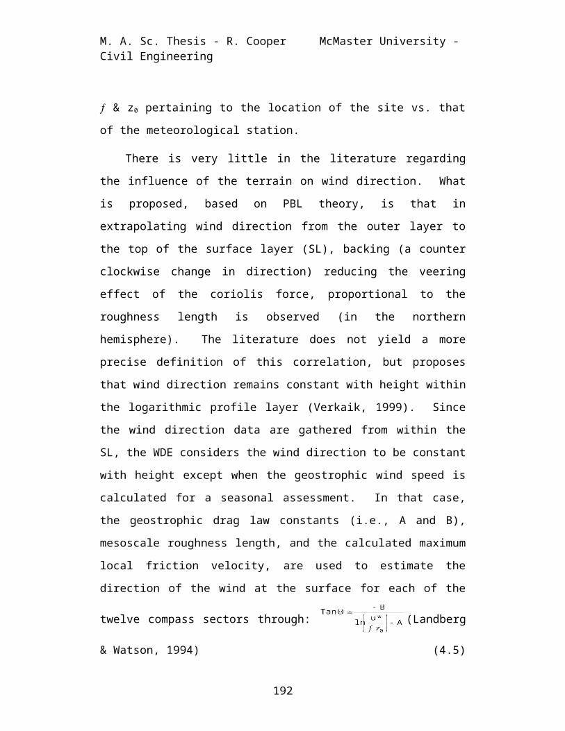
M. A. Sc. Thesis - R. Cooper McMaster University - Civil Engineering
& z0 pertaining to the location of the site vs. that
of the meteorological station.
There is very little in the literature regarding
the influence of the terrain on wind direction. What
is proposed, based on PBL theory, is that in
extrapolating wind direction from the outer layer to
the top of the surface layer (SL), backing (a counter
clockwise change in direction) reducing the veering
effect of the coriolis force, proportional to the
roughness length is observed (in the northern
hemisphere). The literature does not yield a more
precise definition of this correlation, but proposes
that wind direction remains constant with height within
the logarithmic profile layer (Verkaik, 1999). Since
the wind direction data are gathered from within the
SL, the WDE considers the wind direction to be constant
with height except when the geostrophic wind speed is
calculated for a seasonal assessment. In that case,
the geostrophic drag law constants (i.e., A and B),
mesoscale roughness length, and the calculated maximum
local friction velocity, are used to estimate the
direction of the wind at the surface for each of the
twelve compass sectors through: (Landberg
& Watson, 1994) (4.5)
192

M. A. Sc. Thesis - R. Cooper McMaster University - Civil Engineering
In summary, the WDE:
collects (annual option) or calculates (seasonal option) the regional wind statistics;
develops the local wind statistics at the top of the SL, through calculation of the local friction velocity; and
launches the wind data interpolator (WDI).
The function of the WDI will now be discussed.
4.5.2 Wind Data Interpolator
The Wind Data Interpolator (WDI) is the second
submodule of the UWEP module. Its function is to
estimate the mean wind speed profile from the top of
the SL down to the ground. Provided with data from the
Wind Statistics worksheet generated by the WDE and the
Wind Amplifier, the WDI does not require additional
user-interaction. The function of the WDI is
essentially instantaneously completed within the Mean
Wind Speed Profile calculation worksheet when the user
clicks either the OK or Continue button on the Site
Specification form. The profile plot is posted to the
Wind Statistics worksheet. The WDI is established as a
submodule primarily to allow for future modifications
pertaining specifically to equations involving the
estimation of the mean wind speed profile.
193

M. A. Sc. Thesis - R. Cooper McMaster University - Civil Engineering
The WDI is activated three times within the UWEP
module. The first time, the WDI calculates the mean
wind speed profile from the top of the SL down to the
ground, based on the local friction velocity calculated
by the WDE. The second time, the profile is calculated
from the top of the UCL both upward and downward based
on the amplified mean wind speed at the top of the UCL
calculated by the Wind Amplifier in the first stage of
its amplification assessment. Finally, the WDI
generates the profiles associated with the second stage
of the amplification assessment. This section provides
an overview of the key concepts pertaining to the WDI.
Background theory, assumptions, and detailed
calculations are made available through Appendix F.
The mean wind speed profile developed by the WDI is
comprised of the following three SL sublayer-specific
profile segments:
Mesoscale Transitional, and Microscale.
The mesoscale portion pertains to the ISL where z* < z
< zSL, while the microscale portion defines the profile
below the UCL where z zH. The transitional portion
defines the transition between the mesoscale and
194

M. A. Sc. Thesis - R. Cooper McMaster University - Civil Engineering
microscale portions where zH < z < z*. Figure 4.18
depicts the mean wind speed profile as developed
through this multi-layer approach, compared to the
traditional logarithmic profile extrapolation.
195

M. A. Sc. Thesis - R. Cooper McMaster University - Civil Engineering
Figure 4.18. The mean wind speed profile generated bythe WDI.
The profile segments are as follows: solid - logarithmic, diamond- mesoscale, long dash - transitional, and short dash -
196
zSL
zH
z*

M. A. Sc. Thesis - R. Cooper McMaster University - Civil Engineering
exponential. zSL is the height of the top of the SL, z* is theheight of the RSL, and zH is the height of the UCL.
By establishing the complete profile, as opposed to
merely calculating individual mean wind speeds at
specific heights, the WDI provides the Wind Amplifier
submodule with the flexibility to determine the
appropriate reference wind speed for calculating the
amplified mean wind speed at various heights. The wind
speed profile plot is appended to the Wind Statistics
worksheet accessible through the Control Centre.
Activation of the Wind Amplifier submodule and
generation of the wind speed profile essentially occur
simultaneously. The function of, and the required user
inputs for, the Wind Amplifier submodule will now be
discussed.
4.5.3 Wind Amplifier
The Wind Amplifier submodule of the UWEP module
calculates the amplified mean wind speeds and the
characteristic dimensions and areas of the associated
amplification zones. As previously discussed in the
development of the Wind Amplification database, wind
amplification is assessed in two stages. In the first
stage, aerodynamic effect-induced amplification depends
on the configuration of the neighbourhood and the
197

M. A. Sc. Thesis - R. Cooper McMaster University - Civil Engineering
primary and secondary wind directions. In the second
stage, it depends on the subject building and its
individual features.
The user interface within the Wind Amplifier is the
Building Aerodynamics form, including the Neighbourhood
Morphology, Aerodynamic Effects, and Building Feature
subforms. The interaction between the user form,
internal and external databases, and the analysis
worksheet within the Wind Amplifier submodule is
depicted below. The two stages of wind amplification
assessment, including the associated user-input
subforms and worksheets, will now be discussed.
Background theory, assumptions, and detailed
calculations are provided in Appendix G.
W ind Am plifier
W ind Am plificationW orksheet
Urban Param eterisation
Roughness Classification
W ind Am plification
M apQ uest
G oogle M apsBuilding Aerodynam icsAerodynam ic EffectsNeighbourhood M orphologyBuilding Features
Figure 4.19. The Wind Amplifier submodule of the UWEPmodule.
198

M. A. Sc. Thesis - R. Cooper McMaster University - Civil Engineering
For the first stage of the amplification
assessment, the required neighbourhood configuration
and meteorological data are provided to the Wind
Amplifier by the Urban Parameterisation table, the Wind
Statistics worksheet, and the first two tabs of the
Building Aerodynamics form. The Neighbourhood
Morphology tab (Figure 4.20) assists the user in
determining
road classification, and neighbourhood configuration variables.
These characteristics are used by the Wind Amplifier to
reconfigure the inter-building spaces of the urban
subregion selected by the user in the first part of the
assessment.
199
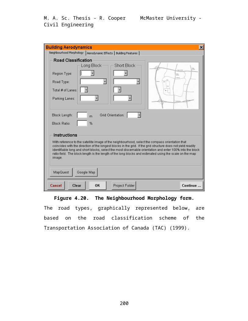
M. A. Sc. Thesis - R. Cooper McMaster University - Civil Engineering
Figure 4.20. The Neighbourhood Morphology form.
The road types, graphically represented below, are
based on the road classification scheme of the
Transportation Association of Canada (TAC) (1999).
200

M. A. Sc. Thesis - R. Cooper McMaster University - Civil Engineering
Figure 4.21. The relationship of urban road typeclassifications.
(TAC, 1999)
Road classification is correlated to street canyon
width [W] within a sub-table of the internal Urban
Parameterisation table, based on the summation of road
type cross-sectional element widths (e.g., the parking
lane, travel lane, sidewalk, etc.). Illustrated below
are the typical cross-sectional elements of an urban,
local, single lane street with two-side parking.
201

LB
SC
W
Sm
SV
M. A. Sc. Thesis - R. Cooper McMaster University - Civil Engineering
Figure 4.22. Typical cross-sectional elements of anurban road.
(Perry & Associates, 2001)
The neighbourhood configuration variables are grid
orientation [] and block
length [Lb], as illustrated.
The block length is the
length of the shortest
block. The longer block
length is calculated by the
Wind Amplifier using the
user-specified block ratio. The block ratio is the
202

M. A. Sc. Thesis - R. Cooper McMaster University - Civil Engineering
ratio of the short block length to the long block
length, expressed as a percentage.
Figure 4.23. Reconfigured cubic array of category # 1.
The user estimates these
variables by referencing
the images of the site's
neighbourhood. These
variables, along with
primary wind direction []
from the Wind Statistics
worksheet and subregion-specific building dimensions
from the Urban Parameterisation table, are used to
estimate the number of streets within the grid and the
angle of flow incidence []. Estimation of the number
of streets within the grid enables the Wind Amplifier
to distinguish inter-building spaces (i.e., the inline
[SV] and orthogonal [SC] space widths) from street
canyon widths [W], as illustrated in Figure 4.23. The
angle of flow incidence [] is defined as the included
angle between the wind direction vector and the grid
orientation vector [], as depicted in Figure 4.24.
Figure 4.24. The critical angles.
The widths and orientations of the spaces dictate the
amplitude and nature of the potential wind
203

M. A. Sc. Thesis - R. Cooper McMaster University - Civil Engineering
amplification. These calculations are performed within
the Amplification Calculations worksheet, which posts
summaries to the Wind Amplification worksheet.
The Aerodynamic Effects tab illustrated below
provides graphical representations of the aerodynamic
effects to assist the user in selecting those that may
be in effect within their site's neighbourhood.
Figure 4.25. The Aerodynamic Effects form.
204

M. A. Sc. Thesis - R. Cooper McMaster University - Civil Engineering
To determine which effects may be applicable, the user
compares satellite images of the site's neighbourhood
obtained from Google Maps and/or MapQuest, with
consideration of the primary and secondary wind
directions, to the portrayed effect images.
Neighbourhood images stored in the Project folder
earlier in the assessment can be accessed through the
Project Folder button. Wind direction data are
obtained from the Wind Statistics worksheet accessed
through the button of the same name or retrieved from
the Canadian Wind Energy Atlas (CWEA).
For each user-selected aerodynamic effect, the Wind
Amplifier compares the calculated inter-building
spaces, angle of flow incidence, and the applicable
urban subregion morphological dimensions against the
critical morphological dimension- and angle of flow
incidence-limits tabulated within the neighbourhood-scale
portion of the Wind Amplification Factor table of the
internal database. If all criteria are met, the
maximum applicable amplification factor is used to
calculate the maximum local gust speed [ ]:
, where: (4.6)
is the maximum amplification factor, and
205

M. A. Sc. Thesis - R. Cooper McMaster University - Civil Engineering
is the reference gust speed based on the
microscale mean wind speed [ ] at the mean
building height of the urban subregion, provided by
the WDI.
The mean wind speed and gust speed can be related to
one other through the wind speed frequency, pdf
parameter(s) (Nigim & Parker, 2007). The Wind
Amplifier provides the amplified local mean wind speed
to the WDI to recalculate the mean wind speed profile.
This step ensures that the appropriate reference wind
speed is available for the second stage of the
amplification assessment. The first stage essentially
recovers a portion of the wind speed lost through the
theoretical extrapolation of the regional wind speed
into the UCL (Christen & Rotach, 2004).
During the second stage, additional potential wind
amplification is assessed based on the dimensions of
the subject building. The wind amplification factors
pertaining to this stage are tabulated by building
surface zone within the Wind Amplification Factor table
of the internal database. For this stage of the
amplification assessment the Building Features tab
illustrated below assists the user in defining the
key dimensions of the subject building, and
206

M. A. Sc. Thesis - R. Cooper McMaster University - Civil Engineering
roof type and orientation.
Figure 4.26. The Building Features form.
207

M. A. Sc. Thesis - R. Cooper McMaster University - Civil Engineering
The key building
dimensions, as
illustrated, are:
eave height [He]or mid-roofheight [Hm],
along-wind depth[D],
cross-windbreadth [B],
buildingorientation [B] or roof ridge orientation [R],
roof type (i.e., flat, hipped, gabled, monoslope, and saw-toothed), and
roof pitch [].
Figure 4.27. Linear and angular building-specificvariables.
If building orientation is not equal to neighbourhood
grid orientation, the angle of flow incidence [] is
redefined as the included angle between the wind
direction vector and the building orientation vector,
as illustrated. The building dimensions are used by
the Wind Amplifier to extract the appropriate values
from the building-scale portion of the Wind
Amplification Factor table and to calculate the
208

M. A. Sc. Thesis - R. Cooper McMaster University - Civil Engineering
corresponding reference height [h], defined within the
National Building Code (NBC). The reference height
determines the height of the reference wind speed,
provided by the WDI, used in the amplification
calculation.
As this appears to be the first attempt at using
published pressure and composite pressure-gust
coefficients to estimate microscale wind amplification,
the reader is directed to Appendix D – 3 for details
pertaining to the assumptions and simplifications
employed by the prototype DSS. The primary limitation
is that peak gusts, to which produce the composite
pressure-gust coefficients pertain, are temporarily
discrete and not necessarily related to the mean wind
speed.
The extracted amplification factors are used by the
Wind Amplifier to calculate the amplified gust speed [
] by building surface zone, defined in the Wind
Amplification Factor table, through , where:
(4.7)
is the reference gust speed, provided by the
WDI based on the neighbourhood-scale amplification
assessment, at the calculated reference height; and
209
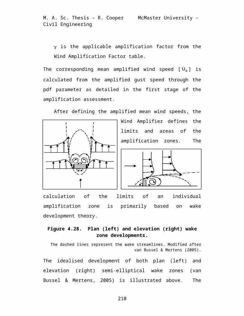
M. A. Sc. Thesis - R. Cooper McMaster University - Civil Engineering
is the applicable amplification factor from the
Wind Amplification Factor table.
The corresponding mean amplified wind speed [ ] is
calculated from the amplified gust speed through the
pdf parameter as detailed in the first stage of the
amplification assessment.
After defining the amplified mean wind speeds, the
Wind Amplifier defines the
limits and areas of the
amplification zones. The
calculation of the limits of an individual
amplification zone is primarily based on wake
development theory.
Figure 4.28. Plan (left) and elevation (right) wakezone developments.
The dashed lines represent the wake streamlines. Modified aftervan Bussel & Mertens (2005).
The idealised development of both plan (left) and
elevation (right) semi-elliptical wake zones (van
Bussel & Mertens, 2005) is illustrated above. The
210

M. A. Sc. Thesis - R. Cooper McMaster University - Civil Engineering
following paragraphs outline the amplification zone
concept. Background theory, assumptions, and detailed
calculations are provided in Appendix G.
Wind amplification is thought to be limited to a
relatively thin band immediately outside of the wake
streamlines illustrated above. The thickness of this
band is approximately 20% of the associated
characteristic dimension (van Bussel & Mertens, 2005).
The characteristic dimension is the building height [H]
for zones above the building corresponding to the
linear dimension of DCt and half the cross-wind
building breadth [B] for
zones on either side of
the building corresponding
to DCs, as illustrated.
The appropriate cross-wind
areas are then calculated
as and
. These areas represent the constant cross-
wind areas of the amplification zones in the along-wind
direction immediately outside of the wake stream line.
The Wind Amplifier calculates the wake streamline
equations, characteristic dimensions, and amplification
zone areas (i.e. side and top) for the four building
211

M. A. Sc. Thesis - R. Cooper McMaster University - Civil Engineering
walls. Detailed calculations are performed in the
Amplification Calculations worksheet, which posts
summaries to the Wind Amplification worksheet.
Figure 4.29. Amplification zones.
To determine whether to calculate a top area [AZt],
side area [AZs], or both, the Wind Amplifier uses the
slenderness ratio [H/B] of the subject building. Cook
(1990) proposes that when 2H/B > 1, the majority of the
wind flows around the sides of the building, while at
2H/B < 1 the majority flows over the building. At 2H/B
1 the wind flows both over and around the building
in a relatively evenly distributed fashion.
In summary, the Wind Amplifier calculates the
amplified mean wind speeds based on the gust speeds and
associated revised pdf parameters, the wake streamline
equations, and the amplification zone areas. Once all
the fields of the Building Aerodynamics form have been
filled, the user instructs the Wind Amplifier to
populate the fields of the Wind Amplification analysis
worksheet and launches the Energy Calculator by
clicking the OK or Continue button. Clicking on the OK
button brings the user back to the Control Centre from
where the worksheets can be reviewed. Clicking the
Continue button generates and opens the Summary Report
212

M. A. Sc. Thesis - R. Cooper McMaster University - Civil Engineering
directly. The function of the Energy Calculator will
now be discussed.
4.5.4 Energy Calculator
The Energy Calculator submodule of the UWEP module
estimates the site's wind energy potential, based on
the amplified mean wind speeds and the amplification
zone areas calculated by the Wind Amplifier. This
submodule does not require a user interface since it
obtains the required data from the worksheets of the
Wind Amplifier and the WDE. All calculations are
performed within the Energy Calculations worksheet with
summaries posted to the Wind Energy worksheet. The
main concepts and equations of the Energy Calculator
will now be discussed. Background theory, assumptions,
and detailed calculations are available through
Appendix H.
The Energy Calculator calculates the theoretical
maximum extractable energy [E] for each building face
by zone (i.e. side and top) through:
, where:
(4.8)
Ei is the wind energy in kWh per time period;
213

M. A. Sc. Thesis - R. Cooper McMaster University - Civil Engineering
i indicates an individual building face zone [AZi],
with each building face having two sides and one
top amplification zone (as illustrated in the last
section of the Wind Amplifier section above);
CP is the coefficient of performance limit (Betz
limit) ~ 0.593;
WPDi is the wind power density in W/m2;
AZi is the amplification zone area in m2;
f()i is the sum of the associated wind direction
frequencies; and
Time Period is one year or one windy season,
depending on whether an annual or seasonal
assessment is being conducted.
The WPD is calculated through: ,
where: (4.9)
is the Rayleigh pdf approximation of the wind
speed frequency distribution: ,
and (4.10)
u is the wind speed class associated with the
frequency.
214

M. A. Sc. Thesis - R. Cooper McMaster University - Civil Engineering
For Equation 4.9, the Rayleigh parameter [b] in
Equation 4.10 is the revised parameter calculated from
the amplified gust speed [ ] by the Wind Amplifier.
The area associated with the building face-specific
amplification zone [AZ] is provided by the Wind
Amplifier. For side amplification zones, as the mean
wind speed varies with height, the pdf parameter
associated with the two-thirds-height mean wind speed
is used in the WPD calculation. Within the literature,
derivation of the Betz limit suggests that the maximum
energy actually available for extraction by a WECS is
approximately 59.3% of the maximum kinetic energy
(Johnson, 2004).
The UWEP module, which contains the WDE, WDI, Wind
Amplifier, and Energy Calculator submodules, stores all
of the data and calculations in the Wind Statistics,
Wind Amplification, and Wind Energy worksheets, from
which the Summary Report is created.
4.6 Summary Report
The Summary Report of the UWEP DSS is generated by
extracting key data and graphs from the Wind
Statistics, Wind Amplification, and Wind Energy
worksheets. The images for the report are obtained
from the Project folder. This report serves two
215

M. A. Sc. Thesis - R. Cooper McMaster University - Civil Engineering
purposes. Primarily, it summarises the site assessment
by identifying the wind energy potential by zone for
the subject site. Secondly, it suggests building
orientation and roof configuration and pitch changes,
which could potentially increase wind amplification
resulting in an increase in the wind energy available
for extraction. If the user is in a position to make
such site adjustments, the Architectural Configurator
connects the user to the appropriate submodule forms
within the UWEP module to do so and rerun the
assessment.
4.7 Architectural Configurator
The Architectural Configurator provides access to
the forms specifically pertaining to building
orientation, roof configuration, and roof pitch data.
It is a structured sub-path within the overall
structure of the UWEP DSS, as illustrated.
Architectural Configurator
Building Aerodynam ics
W ind Am plificationW orksheet
W ind Am plification
W ind EnergyW orksheet
216

M. A. Sc. Thesis - R. Cooper McMaster University - Civil Engineering
Figure 4.30. The Architectural Configurator module ofthe UWEP DSS
The Architectural Configurator can be launched from the
Summary Report or the Control Centre. Once the changes
have been made by the user within the Building
Aerodynamics form, the building-scale stage wind
amplification is reassessed by the Wind Amplifier. The
revised amplified mean wind speeds and amplification
zone areas and characteristics are provided to the
Energy Calculator to recalculate the building zone-
specific, potential wind energy. The Summary Report is
automatically updated.
Within this Chapter the development of the proposed
UWEP DSS was discussed. Lack of similar undertakings
within the literature suggests that this is the first
attempt to develop a prototype DSS in support of
quantifying building aerodynamics-induced wind
amplification for the purpose of estimating wind energy
potential within an urban setting. Unfortunately,
limited suitable data exist in support of validating
the proposed UWEP DSS. Fortunately, time series data
(TSD) collected from a rooftop location on the
University of Toronto's J.P. Robarts Library were made
available. In Chapter 5 the application of the UWEP
DSS to the Robarts Library site, including a comparison
217

M. A. Sc. Thesis - R. Cooper McMaster University - Civil Engineering
of the collected TSD to the wind speeds and directions
calculated by the UWEP module, is discussed. As the
first of two case studies, the Robarts Library site
assessment is intended to lend credibility to the
results generated by the UWEP DSS. The second case
study involves application of the UWEP DSS to determine
the wind energy potential at the site of the Green
Venture Ecohouse.
218

M. A. Sc. Thesis - R. Cooper McMaster University - Civil Engineering
5 APPLICATION OF THE DECISION SUPPORT SYSTEM
The prototype UWEP DSS outlined in Chapter 4 is
believed to be theoretically sound, including the
associated assumptions required to simplify this rather
complex undertaking. To determine whether the
developed tool can yield credible results requires
application of the UWEP DSS in the assessment of
various sites and subsequent comparison of the
calculated values against data collected at these same
sites. Unfortunately, very little suitable urban wind
speed and direction data appear to have been published.
Meteorological stations, for which several decades
worth of data are made readily available, are primarily
located at airports whose terrain characteristics are
not comparable to those of typical urban subregions
(e.g., the categories within the Urban Parameterisation
table of the UWEP DSS). Other urban meteorological
stations collect data at heights above the established
10 m reference height (e.g., Hamilton Royal Botanical
Gardens ID 6153300 ~ 18 m), don't collect wind speed
and direction data (e.g., Toronto City ID 6158355) (EC,
2005d), don't meet the United Nations World
Meteorological Organisation (WMO) Standards (e.g.,
Hamilton Psychiatric Hospital ID 6153298), or are
219

M. A. Sc. Thesis - R. Cooper McMaster University - Civil Engineering
characterised by a combination of the aforementioned.
A tabulation of the historical data collection heights
by station ID for meteorological stations registered
with Environment Canada is provided in Appendix M.
Fortunately, a team of students lead by Barry Rawn
within the Energy Sustainability Community (ESC) of the
University of Toronto (U of T) has been conducting an
assessment of the available wind energy over top of the
Robarts Library on the St. George campus (Rawn, 2006).
In support of this assessment, two years worth of wind
speed and direction data have been collected. This
data, the dimensional details of the Robarts Library,
and preliminary computational fluid dynamics (CFD)
study findings were generously offered in support of
this research undertaking. Although much more data are
required to truly validate the UWEP DSS, this case
study was conducted as a first step in validating the
generated assessment results.
This chapter documents the capabilities of the UWEP
DSS through discussion of two case study applications.
220

M. A. Sc. Thesis - R. Cooper McMaster University - Civil Engineering
Figure 5.1. Robarts Library (left) and the GreenVenture EcoHouse (right).
Photographs are credited to Bell (1978) for the Robarts Libraryand Peterson (2005) for the EcoHouse.
The first case study involves application of the UWEP
DSS in the assessment of the wind energy potential at
the site of the Robarts Library, including a peak
seasonal and a mean annual assessment. The discussion
includes comparison of the amplified mean wind speeds
to the data collected by the U of T's ESC team and a
comparison between the calculated wind power density
(WPD) and the estimate provided by the Canadian Wind
Energy Atlas (CWEA). The second case study pertains to
an assessment of the mean annual wind energy potential
at the site of the Green Venture EcoHouse in Hamilton,
including the selection, siting, and energy generation
potential of appropriate UWECSs.
The chapter is accordingly divided into two
sections pertaining to the institutional and
residential case study applications, respectively.
5.1 Institutional Case Study
The Robarts Library site was selected for the case
study primarily based on the availability of the wind
speed and direction data collected on site. The
221

M. A. Sc. Thesis - R. Cooper McMaster University - Civil Engineering
suitability of an academic campus as a case study site
is further supported by the campus sustainability
movement, which appears to be underway. The Claudette
MacKay-Lassonde Pavilion of the University of Western
Ontario (University of Western Ontario, 2007) and the
Environmental Studies (ES) Green Building of the
University of Waterloo (Office of
Development, University of
Waterloo, 2007) are just a few
examples of green building
projects in support of campus sustainability. The
creation of a Sustainability Office within the Centre
of the Environment at the U of T is yet another example
of campus-based sustainable development. These
initiatives and the multi-disciplinary intellectual
capacity within academia, make a university campus an
ideal site for a case study. This case study will
hopefully act as a catalyst for similar undertakings.
Figure 5.2. The southeast side of the J.P. Robarts Library.In the foreground is the Thomas Fisher Rare Book Library Building;
the head of the peacock (Noyes, 2004).
This case study is documented through two main sections
corresponding to the mean annual and the peak seasonal
energy assessment, respectively. Application of the
222

M. A. Sc. Thesis - R. Cooper McMaster University - Civil Engineering
UWEP DSS to assess the mean annual wind energy
potential at the Robarts Library site will now be
discussed.
5.1.1 Annual Wind Energy Assessment
The mean annual, wind energy assessment portion of
the case study is presented through the following
sections:
Mean wind climate, Amplified mean wind speed, Wind energy, and Summary Report.
These sections will summarise the site-specific user
form data that are provided to the UWEP DSS by the user
and will present tables and graphs summarising the
results at various stages throughout the assessment
process. The detailed calculations, performed within
the calculation worksheets of the UWEP DSS, are
provided as Appendix I - 4 on the compact disc (CD).
5.1.1.1 Mean Wind Climate
The first step of the assessment process involves
the WDE submodule in the determination of the local
wind statistics. During this step the user is required
to fill out the four subforms or tabs of the Site
223

M. A. Sc. Thesis - R. Cooper McMaster University - Civil Engineering
Specification form. The following information is
entered into the fields of the Project Details tab:
Type: Annual Assessment Scope: Site Assessment Project Name: Case Study # 1 - JP Robarts Library Details/Comments: This case study involves the
first step towards validating the UWEP DSS, through the comparison of thecalculated results againstcollected data and CWEA windpower density (WPD) estimates.
In the Site section on the Location
tab, the user enters:
Name: Robarts Library building City: Toronto Province: Ontario Street Address: 130 St. George St. Postal Code: M5S 1A5
Figure 5.3. The John P. Robarts Research Library.(University of Toronto, 2006)
Providing the Geocoder with the address of the Robarts
Library yields the following latitude and longitude co-
ordinates, which the user enters into the corresponding
form fields:
Latitude: 43.664797 ° Longitude: -79.398693 °
224

M. A. Sc. Thesis - R. Cooper McMaster University - Civil Engineering
On the Topographical tab the user is required to
compare the morphology of the campus to the urban
subregion descriptions and characteristics, to
determine which of the urban subregions is most
representative of the campus. To assist the user in
making this comparison, the satellite image of the
campus (Figure 5.4) is obtained by the user using the
satellite imagery application (e.g., Google Maps) and
the address of the Robarts Library. The user is
instructed to save the image to the Project folder of
the UWEP DSS. This comparison suggests that urban
subregion category # 11 is the most representative.
Category # 11 is an urban commercial district
characterised by an average building height greater
than five storeys, a plan area density of 28%, and a
frontal area density of 24%. Category # 13 and # 8,
city centre and mixed commercial / industrial,
respectively could also have been considered but were
dismissed due to their mean building height.
225

M. A. Sc. Thesis - R. Cooper McMaster University - Civil Engineering
Figure 5.4. A satellite image of a portion of the St.George campus.
(Google, 2007)
On the Meteorological tab, the Canadian Wind Energy
Atlas (CWEA) and the Ontario Wind Resource Atlas (OWRA)
buttons link the user to the selected internet-based
wind atlas. For this case study the CWEA is selected
and provided with the site's co-ordinates to obtain the
wind statistics and associated plots at an elevation of
80 m, as illustrated. The user is instructed to save
the wind rose image (Figure 5.5 (b)) to the Project
folder.(a) Mean Wind Speed Histogram (b) Wind Direction Rose
226

M. A. Sc. Thesis - R. Cooper McMaster University - Civil Engineering
Figure 5.5. The wind speed histogram and winddirection rose at 80 m
(EC, 2005a)
With reference to the Turbine formula tab of the Wind rose,
wind speed histogram, turbine formula at a point window, screen-
captured in Figure 5.6 below, the user selects CWEA
from the Data source field options and enters the
following information into the form fields:
Mean: 5.45 m/s Weibull scale parameter: 6.15 m/s Weibull shape parameter: 2.00
227

M. A. Sc. Thesis - R. Cooper McMaster University - Civil Engineering
Figure 5.6. The wind statistics at 80 m (CWEA).
With reference to the data file associated with the
wind rose, available for downloading from the Rose and
histogram tab of the CWEA screen (Figure 5.6), the user
enters the wind direction frequencies for the site into
the compass direction fields, as tabulated below.
Table 5.1. The wind direction frequencies for the
Robarts Library site.
228

M. A. Sc. Thesis - R. Cooper McMaster University - Civil Engineering
N 4.84% S 5.67%NNE 1.05% SSW 13.28%ENE 4.20% W SW 21.08%E 9.04% W 16.99%ESE 4.06% W NW 8.85%SSE 2.61% NNW 8.32%
In selecting the primary and secondary wind directions,
the user should reference the wind rose as opposed to
merely selecting the two directions corresponding to
the highest frequencies. Through grouping cardinal
sectors by quadrant, two to three dominant wind
directions can often be identified for most sites,
which otherwise appear to have relatively omni-
directional frequency distributions. The histogram
plot of the directional frequencies for the Robarts
Library, provided below, perhaps emphasises the tri-
modal nature of the distribution more distinctly than
the wind rose (Figure 5.5 (b)).
0.00%
5.00%
10.00%
15.00%
20.00%
25.00%
W NW NNW N NNE ENE E ESE SSE S SSW W SW WD irection
Frequency %
229

M. A. Sc. Thesis - R. Cooper McMaster University - Civil Engineering
Figure 5.7. Wind direction frequency histogram of theRobarts Library site.
The gridded column represents the primary wind direction,including SSW & W, while the secondary wind directions, diagonal
line columns, are identified as NNW (including WNW & N) and E(including ENE & ESE).
With reference to the wind rose and consideration of
sector combinations as illustrated in Figure 5.7, the
user selects the following directions:
Primary wind direction: WSW Secondary wind direction: E or NNW
A comparison between wind statistics provided by the
OWRA and the CWEA for the Robarts Library site is
summarised in Table 5.2.
Table 5.2. Wind Statistics Summary.
Roughness Length
M ean W ind Speed
z0 (m ) u (m /s) k c (m /s) Prim ary SecondaryOW RA 2.50 4.98 1.97 5.62 SSW NCW EA 2.00 5.45 2.00 6.15 W SW E
Data Source
Elevation (m ) 80
W ind DirectionW eibull Param eters
Once the user has entered the mean wind speed pdf
parameters and the wind direction data, the WDE
calculates the friction velocity within the Wind
230

M. A. Sc. Thesis - R. Cooper McMaster University - Civil Engineering
Statistics worksheet. The friction velocity and urban
subregion category # 11 parameters, stored in the Wind
Statistics worksheet, are used by the WDI to generate
the mean wind speed profile. A copy of the Wind
Statistics worksheet is provided in Appendix I - 1.
The plot of the mean wind speed profile, illustrated
below, is displayed on the Wind Statistics worksheet.
231

M. A. Sc. Thesis - R. Cooper McMaster University - Civil Engineering
232

M. A. Sc. Thesis - R. Cooper McMaster University - Civil Engineering
Figure 5.8. The mean wind speed profile at the RobartsLibrary
At this point the user could choose to continue on
to the wind amplification portion of the assessment or
return to the Control Centre to review the Wind
Statistics worksheet prior to continuing. The wind
amplification portion of the Robarts Library site
assessment will now be discussed.
5.1.1.2 Amplified Mean Wind Speed
During this stage the Wind Amplifier assesses the
potential wind amplification in two stages, requiring
the user to fill out the three subforms of the Building
Aerodynamics form. The first stage of the
amplification assessment re-establishes the true mean
wind speed based on the configuration of the
neighbourhood around the Robarts Library and the
primary and secondary wind directions.
With reference to the map image of the campus
(Figure 5.9), obtained through MapQuest and stored in
the Project folder, the user selects the compass
orientation that coincides with the direction of the
longest blocks in the street grid. If the grid
structure does not yield readily identifiable long and
short blocks, the most discernible orientation is
233

M. A. Sc. Thesis - R. Cooper McMaster University - Civil Engineering
selected and 100% is entered into the block ratio
field. The block length is the average length of the
shorter blocks and the block ratio is the ratio of
short block length-to-long block length, both of which
are estimated using the scale on the map. These
variables define the morphology of the campus. In
summary, the following details are entered into the
appropriate fields on the Neighbourhood Morphology tab:
grid orientation [] NNW block length [Lb] 100 m block ratio 50%
Figure 5.9. Map image of the campus neighbourhood.
This form also contains the Road Classification section
from which the user selects both long block-end and
short block-end, representative street characteristics,
234

M. A. Sc. Thesis - R. Cooper McMaster University - Civil Engineering
with reference to neighbourhood images, the road type
diagram on the form, and/or personal knowledge, as
tabulated below.
Table 5.3. Representative neighbourhood street
characteristics.Long Block Short Block
Region Type - Urban UrbanRoad Type - m inor arterial m ajor arterialLanes # 2 2Parking Lanes # one-side two-sideRoad W idth [W ] m 18.4 24.6
Sussex Ave. Huron St.Harbord St. St. G eorge St.
Characteristics
-Representative block-end Street Nam es
The road width is extracted from a sub-table within the
Urban Parameterisation table, based on the user
selected road classification characteristics. The Wind
Amplifier's redefinition of the inter-building spaces
and the angles of flow incidence for the Robarts
Library neighbourhood are tabulated below. These
values assist in determining whether a particular
aerodynamic effect could be producing neighbourhood-
scale amplification on campus.
Table 5.4. Neighbourhood inter-building spaces and
angles of flow incidence.
235

M. A. Sc. Thesis - R. Cooper McMaster University - Civil Engineering
O rthogonal In-line M inim um Angle of Flow Incidence
SC SV Sm
(degrees)17.5 13.2 0.6 90
(m )
Inter-building Space W idth
The Aerodynamic Effects tab provides selectable
illustrations of the aerodynamic effects tabulated
within the Wind Amplification Factor table to assist
the user in identifying the potentially applicable
effects. Selection is based on a comparison between
the presented images and the images of the campus,
further enhanced by user-knowledge of the area. The
Wind Amplifier compares the critical values of the
user-selected aerodynamic effects, tabulated within the
Wind Amplification Factor table, against the campus'
inter-building spaces and angles of flow incidence
(Table 5.4) to determine the maximum applicable
amplification factor. Based on this comparison, the
tower effect is selected, resulting in the calculation
of the maximum local gust speed [ ] and amplified mean
wind speed [ ] as tabulated below. The amplified
mean wind speed is provided to the WDI to regenerate
the amplified mean wind speed profile, as illustrated
in Figure 5.10.
236

M. A. Sc. Thesis - R. Cooper McMaster University - Civil Engineering
Table 5.5. Summary of the first stage of the
amplification assessment.MeanWindSpeed
Gustspeed
Amplification Factor
GustSpeed
Mean WindSpeed
(H) (H) (H) (H)(referen
ce)(referen
ce)(towereffect)
(localmaximum)
(amplified)
m/s m/s - m/s m/s1.39 2.22 1.82 4.05 2.54
All wind speeds are at the mean building height [H] of 21 massociated with urban subregion category # 11.
237

M. A. Sc. Thesis - R. Cooper McMaster University - Civil Engineering
238

M. A. Sc. Thesis - R. Cooper McMaster University - Civil Engineering
Figure 5.10. The amplified vs. the original mean windspeed profile.
The mean building height [H] of the representative
urban subregion is 21 m, while the eaves height [He] of
the Robarts Library is 80 m. As such, neighbourhood
morphology-induced wind amplification is not considered
to be present at the roof height of the Robarts
Library, but is considered to exist at heights below
twice the mean building height of the representative
urban subregion category (i.e. 2H = 42 m).
In the second stage of the amplification assessment
the user selects the appropriate roof type and provides
the following key building dimensions through the
Building Features subform:
building eaves height [He] = 80 m along-wind depth [D] = 102 m cross-wind breadth [B] = 91 m building orientation [B] = NNW roof ridge orientation [R] = N/A roof type ~ flat roof slope [] = 0
239

M. A. Sc. Thesis - R. Cooper McMaster University - Civil Engineering
Figure 5.11. The plan and elevation views of theRobarts Library.
On user-selection of the flat roof type, the roof ridge
orientation field and roof pitch fields automatically
equate to N/A and 0, respectively. The appropriate
cross-wind breadth is identified by recalling that the
primary wind direction is out of the WSW, with
reference to the plan view of the Robarts Library. The
depth is then defined as the dimension perpendicular to
the breadth. The UWEP DSS transforms this triangular
building into its rectangular cross-wind equivalent, as
illustrated below.
240

M. A. Sc. Thesis - R. Cooper McMaster University - Civil Engineering
Figure 5.12. The UWEP DSS cubic representation of theRobarts Library.
The block arrows indicate the building face designations assignedby the Wind Amplifier.
Using the information provided through the Building
Features tab, the Wind Amplifier selects the
appropriate amplification factor(s) from the Wind
Amplification Factor table of the internal database.
The pertinent portion of the flow chart of this
selection process is illustrated below, where I -15
corresponds to the pressure coefficient plot (Figure I-
241

M. A. Sc. Thesis - R. Cooper McMaster University - Civil Engineering
15) from the National Building Code (NBC) (Canadian
Commission on Building and Fire Codes, 2006).
W hole Building
Building Structure
I - 15
~ 90
building surface
N/A
He 20 m No
No
Figure 5.13. The decision process of the WindAmplifier.
I - 15 corresponds to Figure I - 15 from Commentary I of the NBC.
The building surfaces, from this portion of the Wind
Amplification Factor table, are the edge-zones of the
three surfaces perpendicular to an associated windward
building face (i.e., the roof and both sides) as
illustrated below.
242

M. A. Sc. Thesis - R. Cooper McMaster University - Civil Engineering
Figure 5.14. Isometric representation of the buildingsurface zones.
FS is the frontal stagnation point, above which the wind primarilyflows over the top of the building.
Table 5.6 summarises the amplification factors and
building-scale, amplified mean wind speeds for the side
and top surfaces of the four faces of the cuboidal
representation of the Robarts Library.
Table 5.6. Summary of the second stage of the
amplification assessment.MeanWindSpeed
Amplification Factor AmplifiedMean Wind Speed
243

M. A. Sc. Thesis - R. Cooper McMaster University - Civil Engineering
(He) (h)(referen
ce)(side) (top) (side) (top)
m/s - - m/s m/s5.45 1.43 1.58 7.35 8.62
h is the reference height = He (eave height of the RobartsLibrary) for the top and the mid-point of the upper third of the
eaves height (i.e. 67 m) for the side.
Figure 5.15 provides a comparison between the amplified
reference profile and the additional amplification
along side and overtop of the building faces of the
Robarts Library.
244

M. A. Sc. Thesis - R. Cooper McMaster University - Civil Engineering
Figure 5.15. The amplified wind speed profiles aroundthe Robarts Library.
In the final step of the amplification assessment
the Wind Amplifier submodule calculates the critical
245

M. A. Sc. Thesis - R. Cooper McMaster University - Civil Engineering
slenderness ratio of the Robarts Library, the
characteristic dimensions, amplification zone areas,
and the equations for the semi-elliptical wake
streamlines. These calculations are made for each
building face, as tabulated below, based on the
building dimensions.
Table 5.7. Characteristic dimensions and amplification
zone areas.Slenderness Ratio [2H/B] : 1.76
Side Characteristic Dim ension
Top Characteristic Dim ension
Side Am plification Zone Area
Top Am plification Zone Area
D Cs D Ct AZs AZt
- m m m 2 m 2
NW 10.2 16.0 816 1632SW 9.1 16.0 728 1456SE 10.2 16.0 816 1632NE 9.1 16.0 728 1456
Building Face
The wake streamline equations position the
amplification zones in relation to the sides and the
top of the building (Cook, 1990). The wake streamline
plots are provided in Appendix J - 1b. The slenderness
ratio suggests that the wind will primarily flow around
the sides except near the top of the building above the
frontal stagnation (FS) point (Figure 5.14). The FS
point, typically at 2/3H, is the theoretical point at
which the free stream wind velocity is brought to rest,
corresponding to u = 0 m/s and CP = 1 (Cook, 1985).
246

M. A. Sc. Thesis - R. Cooper McMaster University - Civil Engineering
The amplification zone areas are quite large due to the
size of the Robarts Library, which is directly
proportional to the characteristic dimensions used to
calculate these areas.
Ideally, appropriately dimensioned, modular UWECSs
would be mounted both on top and along side of the
Robarts library. The appropriate dimensions are
defined as the characteristic dimensions of the UWECS,
which would produce an area taking up as much of the
amplification zone area as possible. For a horizontal
axis wind turbine (HAWT) the characteristic dimension
is the rotor diameter [RD] and the area, or swept area
[AS], is equal to .
Vertical axis wind turbines (VAWTs) are typically
based on either the Savonius (Figure 1.11a) or the
Darrieus (Figure 1.11b) configuration. The
characteristic dimensions are
the rotor diameter and the
rotor height [RH]. The area of
a Savonius VAWT is equated to
. For a Darrieus-based
VAWT the area is estimated as
247

M. A. Sc. Thesis - R. Cooper McMaster University - Civil Engineering
(D. L. Miller, 1981). Variations on the Darrieus
configuration have been developed, which straighten out
the sides of the classic egg beater shape.
Consequently, this configuration of VAWT is often
called an H-Darrieus (Mertens, van Kuik, & van Bussel,
2003a; Mertens, van Kuik, & van Bussel, 2003b) an
example of which is Turby®, illustrated in Figure 5.16.
Figure 5.16. Turby® - An H-Darrieus VAWT
The area of an H-Darrieus VAWT is (van Bussel,
Mertens, Polinder, & Sidler, 2004).
At the end of the amplification assessment the Wind
Amplifier returns the user to the Control Centre. No
further user input is required for the Energy
Calculator submodule of the UWEP module.
5.1.1.3 Wind Energy
The Energy Calculator calculates the theoretical
maximum extractable energy [Ei] for each building face
by zone [AZi] (i.e., side and top) using Equation
(5.1).
, where: (5.1)
Ei is the wind energy in Wh per time period;
248

M. A. Sc. Thesis - R. Cooper McMaster University - Civil Engineering
i indicates an individual building face zone [AZi],
with each building face having two sides and
one top amplification zone (as illustrated in
Figure 5.14);
, where: (5.2)
CP is the coefficient of performance ~ 0.593
(Betz limit);
is the wind power density in
W/m2, with f(u) representing the wind speed
frequency distribution;
AZi is the amplification zone area in m2;
f()i is the sum of the wind direction
frequencies associated with the wind
directions considered orthogonal to a
particular building face; and
Time Period is one year or one windy season,
depending on whether an annual or seasonal
assessment is being conducted.
The theoretical maximum wind power density (WPD) and
wind power available for extraction at the Robarts
Library by building face and zone are summarised below.
249

M. A. Sc. Thesis - R. Cooper McMaster University - Civil Engineering
Table 5.8. Wind power by building face and zone at the
Robarts Library.
W PD NW SW SE NEZone W /m 2
Side 442.8 47.2 98.2 26.4 27.3Top 707.2 150.6 313.5 84.5 87.3
Building Face
Pow er [P] (kW )
Values corresponding to the side zone are per-side values. The topis at 80 m and the side is at 67 m.
The values are higher within the top zones, since
wind speed increases with height and the top wind
amplification factor is larger than the one applied at
the side of the building. The variation between faces
is due to differing amplification zone areas and the
corresponding wind direction frequencies. As
previously mentioned, the power is based on the
idealised assumption that the UWECS can occupy the
entire amplification zone area. Based on the
aforementioned assumption, the theoretical maximum
extractable energy per building face and zone per year
is summarised in Table 5.9. An appropriately
configured UWECS could conceivably extract wind energy
from both sides of a building face, all faces at the
top edges, etc., in which case it would generate a
summation of the corresponding tabulated values for the
entire building. A comparison of the potentially
250

M. A. Sc. Thesis - R. Cooper McMaster University - Civil Engineering
extractable energy vs. the energy needs of this
building is beyond the scope of this research
undertaking.
Table 5.9. Mean annual wind energy by building face
and zone.
NW SW SE NEZoneSide 413.1 859.9 231.6 239.3Top 1319.6 2746.6 739.8 764.3
Energy [E] (M W h per year)
Building Face
At this point the UWEP module has completed its
tasks within the assessment process and the user is
presented the Summary Report.
5.1.1.4 Summary Report
The Summary Report summarises the assessment
findings, including details pertaining to building
features and/or orientation changes that could
potentially increase the wind energy available for
extraction. The Summary Report in its entirety is
provided in Appendix J - 1.
Unfortunately, the changes suggested by the UWEP
DSS primarily involve roof type and pitch
modifications, which are limited to low-rise buildings
(i.e., He < 20 m) due to NBC data limitations. If low-
251
M. A. Sc. Thesis - R. Cooper McMaster University - Civil Engineering
rise, roof-related NBC data can be considered
transferable to high-rise buildings, retrofitting the
Robarts Library with a sawtoothed roof could
conceivably increase the roof top amplification from
the maximum of 1.58 to 1.71. This would result in a
greater than 25% increase in available wind energy for
extraction. Based on the cubic representation of the
subject building, the building is sub-optimally
oriented. If its largest face, as opposed to its
smallest, were perpendicular to the primary wind
direction, the size of the amplification zone area
orthogonal to the primary wind direction would be
increased. An increase in amplification zone area
allows for a larger UWECS to be installed and more
energy to be extracted. Considering the true
triangular shape of the building, the prevailing winds
out of the SSW and E impinge on building corners. The
nature of the flow field above and around building
corners will be explored in the Discussion section of
this chapter.
One of the shortcomings of an annual assessment
using the wind atlases is that the atlases do not
correlate wind speed frequency to wind direction.
Traditional, tower mounted, horizontal-axis wind
turbines (HAWT) are equipped to align themselves with
252

M. A. Sc. Thesis - R. Cooper McMaster University - Civil Engineering
the wind direction, but due to the size of modern day
turbines, additional external energy is most often
required to do so. Building mounted or augmented wind
turbines (BUWTs), if primarily based on the vertical
axis wind turbine (VAWT) configuration, can utilise
wind from all directions without needing to change
their position, but building-integrated systems are
usually bi-directional or unidirectional. In the
latter case, determination of which sectors yield the
most energy is of utmost importance. This is achieved
by using the UWEP DSS to conduct a seasonal assessment,
as will now be discussed.
5.1.2 Seasonal Wind Energy Assessment
The seasonal mean wind energy assessment of the
Robarts Library site primarily differs from the annual
assessment within the WDE submodule of the UWEP DSS,
affecting wind amplification and the resulting wind
energy potential. This portion of the case study is
accordingly presented through the following sections:
Mean wind climate, Wind Amplification, and Energy calculation.
Unlike an annual assessment, a seasonal assessment
allows the user to identify which months are
253

M. A. Sc. Thesis - R. Cooper McMaster University - Civil Engineering
characterised by higher mean wind speeds and the
corresponding peak energy available for extraction
during these months. Throughout this discussion these
months will be collectively referred to as the windy
season. The time series data (TSD) available for a
seasonal assessment also allow for the correlation
between wind speed and wind direction to be determined.
Establishing this correlation yields more accurate
energy estimations since direction-specific mean wind
speed distributions are used in the calculations.
During an annual assessment, due to wind atlas
limitations, the UWEP DSS assigns the same wind speed
frequency distribution to each wind direction sector
when calculating the potential energy.
A seasonal assessment is based on mean hourly data
over a twelve month period. If the site is located in
Ontario the OWRA can be used to identify the windy
season, reducing the amount of data that need to be
downloaded from the climate data archive. The steps
specific to the seasonal assessment of the Robarts
Library site will now be discussed.
5.1.2.1 Mean Wind Climate
When a seasonal assessment is being conducted, the
initial differences are observed in the Meteorological
254

M. A. Sc. Thesis - R. Cooper McMaster University - Civil Engineering
tab of the Site Specification form. This subform is
different from the one presented during an annual
assessment. For the Robarts Library site, the seasonal
assessment is simplified by determining which months
constitute the windy season using the graph obtained
through the OWRA, illustrated below.
With reference to the monthly mean wind speed
graph, the user selects: November, December, and
January from the drop down menus in the Windiest Months
section of the form. Accessing the CWEA, the following
additional information is entered:
Roughness Length: 2 m Station Name: Toronto Island Airport Latitude: 43.630 Longitude: -79.400
Figure 5.17. Monthly regional mean wind speedvariation.
255

M. A. Sc. Thesis - R. Cooper McMaster University - Civil Engineering
Using the Atlas the land-use in the vicinity of the
meteorological station is approximated to 'Built
features, semi-rough (e.g., airport, including
buildings & trees)', which the Roughness Classification
table equates to a roughness length of 0.03 m. Using
the co-ordinates of the Robarts Library and those of
the Toronto Island airport, the WDE calculates that the
meteorological station is approximately 4 km from the
Robarts Library. As such, the wind statistics from the
meteorological station are used to calculate the
mesoscale wind statistics at 80 m.
The user obtains the mean hourly TSD recorded at
the meteorological station of the Toronto Island
Airport (TIA) from the National Climate Data &
Information Archive (NCD&IA) website. Pasting a
concatenation of the three months of wind speed and
direction data into the appropriate columns of the
Windy Season Statistics Calculations worksheet,
calculates the mesoscale regional wind speed for each
of the twelve cardinal sectors of the season and
produces the associated wind direction rose. The wind
direction rose for the windy season is illustrated
below. The mean wind speed during the windy season was
found to be 1.3X the mean annual wind speed, based on
256

M. A. Sc. Thesis - R. Cooper McMaster University - Civil Engineering
the hourly TSD collected at 10 m at the TIA for the
year 2005.
0.0%5.0%10.0%15.0%20.0%25.0%
N
NNE
ENE
E
ESE
SSE
S
SSW
W SW
W
W NW
NNW
Figure 5.18. The windy season wind rose at the TorontoIsland Airport .
During a seasonal assessment the wind speed
frequency distribution is determined for each of the
twelve cardinal sectors for each month or the windy
season. This case study only involves assessment of
the windy season. Figure 5.19 illustrates the
variation in the sector-specific, wind speed frequency
distributions, by comparing ESE, the direction from
where the lowest mean wind speed is expected, against
ENE and WSW from where the highest mean wind speeds
originate. The wind speed distribution produced by
combining all directions, represented by All in Figure
257

M. A. Sc. Thesis - R. Cooper McMaster University - Civil Engineering
5.19, yields a mean wind speed of ~ 21% less than the
highest mean wind speed associated with the WSW
direction. In other words, the mean wind speed out of
the WSW is ~ 1.26X the windy season mean wind speed.
Since wind energy is proportional to the wind speed
cubed, depending on the direction-specific frequency
distributions and the associated mean wind speeds,
using the windy season mean wind speed to calculate the
wind energy potential could result in an
underestimation by a factor of 2. The potential wind
energy calculated using individual direction-specific
wind speed distributions and the associated directional
frequencies was estimated to be ~ 6% greater than that
calculated based on the windy season mean wind speed
occurring 100% of the time.
258

M. A. Sc. Thesis - R. Cooper McMaster University - Civil Engineering
0%
10%
20%
30%
40%
50%
60%
70%
0 1 2 3 4 5 6 7 8 9 10W ind Speed Class (m /s)
Frequency %
W SW ESE ENE All
Figure 5.19. The windy season wind speed distributionby direction at 21 m.
The WDI generates the mean wind speed profiles at
the site for all twelve of the cardinal sectors. The
mean wind speed profiles corresponding to winds out of
the ENE and WSW at the Robarts Library site are
depicted below. These cardinal sector-specific
profiles are used by the Wind Amplifier to determine
the appropriate reference wind speed during the wind
amplification assessment.
259

M. A. Sc. Thesis - R. Cooper McMaster University - Civil Engineering
Figure 5.20. The ENE & WSW mean wind speed profiles.
260
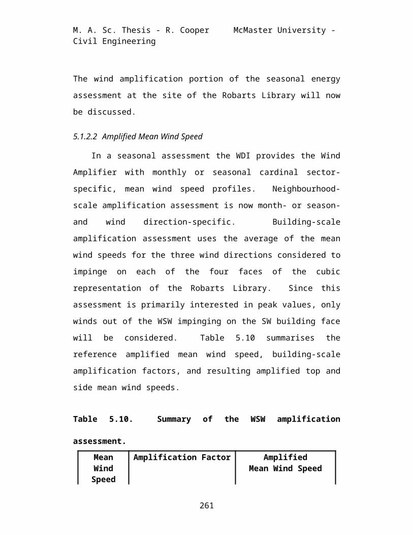
M. A. Sc. Thesis - R. Cooper McMaster University - Civil Engineering
The wind amplification portion of the seasonal energy
assessment at the site of the Robarts Library will now
be discussed.
5.1.2.2 Amplified Mean Wind Speed
In a seasonal assessment the WDI provides the Wind
Amplifier with monthly or seasonal cardinal sector-
specific, mean wind speed profiles. Neighbourhood-
scale amplification assessment is now month- or season-
and wind direction-specific. Building-scale
amplification assessment uses the average of the mean
wind speeds for the three wind directions considered to
impinge on each of the four faces of the cubic
representation of the Robarts Library. Since this
assessment is primarily interested in peak values, only
winds out of the WSW impinging on the SW building face
will be considered. Table 5.10 summarises the
reference amplified mean wind speed, building-scale
amplification factors, and resulting amplified top and
side mean wind speeds.
Table 5.10. Summary of the WSW amplification
assessment.MeanWindSpeed
Amplification Factor AmplifiedMean Wind Speed
261

M. A. Sc. Thesis - R. Cooper McMaster University - Civil Engineering
(H) (h)(referen
ce)(side) (top) (side) (top)
m/s - - m/s m/s4.90 1.43 1.58 14.17 16.61
The reference height [h] is 80 m for the building-top zone and 67m for building-side zone.
The amplified reference profile and the along side and
overtop profiles resulting from building-scale
amplification associated with the SW building face of
the Robarts Library are depicted in Figure 5.21 below.
262

M. A. Sc. Thesis - R. Cooper McMaster University - Civil Engineering
Figure 5.21. The WSW peak seasonal and amplified windspeed profiles.
The amplification zone areas and wake streamline
equations are the same as in an annual assessment. The
263

M. A. Sc. Thesis - R. Cooper McMaster University - Civil Engineering
peak seasonal potential wind energy at the Robarts
Library site will now be discussed.
5.1.2.3 Wind Energy
In a seasonal assessment, wind energy is calculated
based on a unique wind speed distribution for each of
the twelve cardinal sectors. Since the case study is
interested in peak seasonal values, the wind power
density (WPD), power, and energy per zone associated
with winds out of the WSW are tabulated below. The
power and energy calculations take into account the
frequency of winds originating out of the WSW.
Table 5.11. The peak season contributions from the WSW
wind direction.
W ind Power Density
Power Energy
W PD [P] [E](W /m 2) (kW ) (M W h / yr)
Side 2037.5 186.9 1637.3Top 2303.8 422.7 3702.7
Zone
Building FaceSW
The peak mean seasonal energy potential associated
with winds out of the WSW overtop of the SW face of the
Robarts Library is approximately 3X greater than the
mean annual associated with the same wind direction.
264
M. A. Sc. Thesis - R. Cooper McMaster University - Civil Engineering
Given that wind energy is proportional to the wind
speed cubed, this finding suggests that the windy
season mean amplified wind speed is ~ 1.4X the mean
annual wind speed. Considering that the windy season,
mean wind speed without amplification was previously
determined to be 1.3X the mean annual wind speed and
that 2 - 3X amplification has been found to exist, the
potential peak mean seasonal energy estimation is quite
reasonable.
The Summary Report for a seasonal assessment is
primarily the same as the one generated for the annual
assessment, except that it provides seasonal and/or
monthly estimates vs. mean annual. This added level of
detail is considered crucial in the development of
hybrid solar-wind energy conversion systems, since wind
speeds are typically higher during seasons when solar
radiation levels are lower. It also assists in
determining the most promising cardinal sectors for
uni- or bi-directional, building-integrated UWECS
installations.
This concludes the application of the UWEP DSS to
the case study of the wind energy potential at the site
of the Robarts Library. Prior to delving into the
second case study, a discussion regarding the validity
265

M. A. Sc. Thesis - R. Cooper McMaster University - Civil Engineering
of the results generated by the UWEP DSS application is
provided. In the following section, a comparison
between the amplified mean wind speed as calculated by
the UWEP DSS and the data provided by the U of T team
will be discussed, including directional persistence
and seasonal influences. The section also includes a
comparison between the calculated wind power density
(WPD) and the estimated WPD proposed by the wind
atlases and the limitations of the UWEP DSS with
respect to the case study application.
5.1.3 UWEP DSS Credibility Investigation
This discussion section is primarily intended to
lend credibility to the results produced by the UWEP
DSS in assessing the wind energy potential at the site
of the Robarts Library. To that end, the time series
data (TSD) collected by the roof-mounted anemometer and
wind direction vane were analysed to determine the mean
wind speeds and dominant wind directions on the roof of
the Robarts Library.
The NRG#40 anemometer and NRG #200P direction vane
were mounted near the mechanical room of the southwest
penthouse, approximately 9.8 m above the main roofline
of the Robarts Library. The accuracy of the anemometer
is 0.1 m/s for wind speeds ranging from 5 m/s to 25
266

M. A. Sc. Thesis - R. Cooper McMaster University - Civil Engineering
m/s and undefined below 4 m/s (Gee, 2007). The
accuracy of the wind direction vane is 3.6. In
Figure 5.22, the location of the instrumentation is
indicated by the star in the satellite image plan view.
The arrow on top of the Bahen Centre is from where the
photograph was taken, with the cross hairs indicating
the approximate location of the anemometer. The
simplified elevation sketch corresponds to the
photograph, with the mechanical room portion of the
southwest penthouse detailed in the lower left image.
267

M. A. Sc. Thesis - R. Cooper McMaster University - Civil Engineering
Figure 5.22. Instrumentation placement on thesouthwest penthouse.
This discussion is presented through the following
sections:
Mean wind climate, Wind power density, and Limitations.
5.1.3.1 Mean Wind Climate
The analysis of the time series data (TSD)
collected by the roof-mounted anemometer proved
problematic. Unfortunately, even though mean minutely
data were collected for almost a year and a half, no
data were collected through the summer during either
year and some months were too incomplete to be
considered in the comparison. With the summer season
data missing, the mean annual wind speed could not be
determined from the data provided. As such, the
268

M. A. Sc. Thesis - R. Cooper McMaster University - Civil Engineering
comparison is limited to the months identified as
corresponding to the highest mean wind speed. Figure
5.23 depicts the mean wind speed by month as calculated
from the TSD collected during 2005 and 2006.
0
1
2
3
4
5
6
7
Jan Feb M ar Apr M ay Jun Jul Aug Sep O ct Nov D ec
Mean Wind Sp
eed [u] (m/s)
2005 2006-Inc. 2005-Inc. 2006
Figure 5.23. Robarts Library Monthly mean wind speed.Chart Notes: No data were collected in 2005 between Apr and
August, inclusive. Data collection stopped at the end of May in2006. In 2005 the incomplete months (diagonal-hatch) were Feb and
Mar at 2.8% and 0.1% complete, respectively. In 2006 theincomplete months (horizontal-hatch) were Jan and May at 33.3% and
27.0% complete, respectively.
Considering only the months with greater than 80%
complete data sets, November, December, and February
were identified as the months during which the highest
mean wind speeds occurred. The mean wind speed for
February was greater than that for January, identified
by the OWRA in the seasonal assessment, possibly due to
the fact that the data set for January was only 81.2%
269

M. A. Sc. Thesis - R. Cooper McMaster University - Civil Engineering
complete. The data sets for all the other months
plotted in Figure 5.24 were greater than 95% complete.
The mean wind speed during the windy season was
calculated to be 5.62 m/s.
0
1
2
3
4
5
6
7
Jan Feb M ar Apr Sep O ct Nov D ec
Mean Wind Sp
eed [u] (m/s)
~ 85% W indy Season > 95%
Figure 5.24. Monthly mean wind speed (>80% completemonths).
The column fill indicates: less than 85% complete data set (hatch-marks), greater than 95% (grey), and highest mean wind speed
(black).
Wind direction data were limited by the same
findings as previously detailed pertaining to wind
speed data. Defining the windy season as the three
months during which the highest mean wind speeds were
recorded, as identified in Figure 5.24, the wind
direction rose illustrated below suggests that the
270

M. A. Sc. Thesis - R. Cooper McMaster University - Civil Engineering
primary and secondary wind directions during this
season are NNW/N and S, respectively.
0.0%
5.0%
10.0%
15.0%
20.0%
25.0%N
NNE
ENE
E
ESE
SSE
S
SSW
W SW
W
W NW
NNW
W indy Season TIA veered 90 deg
Figure 5.25. The windy season wind rose vs. TIA dataveered 90 degrees.
Though the same three dominant directions were
identified through analysis of the Toronto Island
Airport (TIA) windy season data, the primary direction
identified from the Robarts Library data is the
direction identified as tertiary at the TIA. There are
several possible explanations for this observation.
Firstly, measurement instrument resolution, the
number of cardinal sectors into which data are
categorised, and definition of category limits can have
271

M. A. Sc. Thesis - R. Cooper McMaster University - Civil Engineering
a profound effect on the identification of primary and
secondary wind directions. Figure 5.26 illustrates how
categorising the wind direction frequencies into four
inter-cardinal directions, as opposed to twelve, NW
emerges as the secondary wind direction for the TIA and
CWEA data vs. E or ENE.
0.0%
5.0%
10.0%
15.0%
20.0%25.0%
30.0%
35.0%
40.0%
45.0%
50.0%
SW NW NE SEDirection
Frequency %
TIA W indy Season RL W indy Season CW EA Annual
Figure 5.26. Wind direction frequency comparison.The abbreviations are TIA = Toronto Island Airport, RL = Robarts
Library, and CWEA = Canadian Wind Energy Atlas.
The Robarts Library wind direction data are in degrees
to four decimal places and the Toronto Island Airport
data are in tens of degrees. The UWEP DSS categorises
TSD into twelve cardinal sectors, centering each sector
within the category limits (i.e., 15 N > 345).
With the TIA data provided in tens of degrees, it is
conceivable that directional data may have been skewed
272

M. A. Sc. Thesis - R. Cooper McMaster University - Civil Engineering
by 5 due to the category limit definitions of the UWEP
DSS. The CWEA groups the frequencies into twelve
cardinal sectors, but does not provide details
regarding category limit definitions.
Secondly, if the TIA wind rose for the same three
months is veered 90 (clockwise) or backed 270, a very
similar wind direction frequency distribution can be
created, as depicted in the dashed-line wind rose
overlay in Figure 5.25. In the northern hemisphere an
increase in friction, represented by an increase in
roughness length in wind power meteorology, causes a
counter-clockwise change in the wind direction or
backing. This finding suggests that the net change in
roughness length between the airport and the Robarts
Library and the height differential (i.e., 10 m at the
airport vs. 80 m at the library) may have combined to
result in either veering or backing of the wind
direction at the data collection site.
Lastly, perhaps the data were collected within
penthouse- and/or building corner-induced wakes below
the wake streamline, characterised by turbulence and
vortices. The reduced mean wind speed observed during
the windy season on the roof of the Robarts Library
compared to that calculated by the UWEP DSS from the
273

M. A. Sc. Thesis - R. Cooper McMaster University - Civil Engineering
Toronto Island Airport (TIA) TSD at 80 m, suggests that
the measurement location was perhaps suboptimal within
the aforementioned wake zones.
0%
2%
4%
6%
8%
10%
12%
14%
16%
0 2 4 6 8 10 12 14 16 18 20 22 24 26W ind Class (m /s)
Frequency %
Robarts W indy Season @ 90 m
TIA W indy Season @ 80 m
Figure 5.27. The windy season wind speed distributioncomparison.
TIA data are from the Toronto Island Airport meteorologicalstation at 80 m, while Robarts data are at ~ 90 m.
Considering only the primary and secondary wind
directions, the Robarts Library data once again yield
slightly lower mean wind speeds even though the data
were collected at ~ 89 m, while the TIA data were
measured at 10 m at the Toronto Island Airport (TIA)
and extrapolated to 80 m.
274

M. A. Sc. Thesis - R. Cooper McMaster University - Civil Engineering
0%
2%
4%
6%
8%
10%
12%
14%
16%
0 2 4 6 8 10 12 14 16 18 20 22 24 26W ind Class (m /s)
Frequency %
Robarts Prim ary W ind Direction
Robarts Secondary W ind Direction
TIA Prim ary W ind Direction
TIA Secondary W ind Direction
Figure 5.28. The primary & secondary direction windspeed distributions.
The profiles associated with the primary and secondary winddirections are represented by the solid lines and dashed lines,
respectively, with diamond markers for the TIA-based data. The TIAdata are the 80 m un-amplified, while the Robarts data are at ~ 90
m.
The supposition that the data were collected below
the wake streamline is thus far supported by the wind
direction discrepancies and the 89 m mean wind speeds
being lower than even those observed at an elevation of
10 m at the Toronto Island Airport. Further support of
this assumption is provided by the wake development
theory-based stream line equations. Considering winds
out of the WSW and the position of the anemometer at
47.4 m downstream of the roof's edge, wake development
theory suggests that the height of the wake stream line
275

M. A. Sc. Thesis - R. Cooper McMaster University - Civil Engineering
at the location of the anemometer is ~ 17.5 m above the
eaves height of the Robarts Library. The anemometer
collecting the data was mounted at ~ 10 m above the
eaves height, conceivably well within the wake.
Initial computational fluid dynamics (CFD)
investigation of a portion of the Robarts Library
subjected to 10 m/s winds out of the SSW (Figure 5.29)
also indicates that the anemometer may be situated
within the turbulent region of initial flow separation.
In the side view of the Robarts Library CFD model
(Figure 5.29 b)), the instrumentation is possibly
located in the green area where a 30% reduction in the
free stream wind speed is expected.
(a) Frontal view.
276

M. A. Sc. Thesis - R. Cooper McMaster University - Civil Engineering
(b) Side View
Figure 5.29. Computational fluid dynamics modelscreated by CFX.
The free stream wind speed was set to 10 m/s for the computationalanalysis. Wind amplification up to 1.4X the free stream wind speedwas predicted by the model above and to the sides of the RobartsLibrary when subjected to skewed flow. The cross hairs on the
inset image represent the approximate location of the anemometerand direction vane (Rawn, 2006).
277

M. A. Sc. Thesis - R. Cooper McMaster University - Civil Engineering
Table 5.12 summarises the mean annual and windy
season mean wind speeds and directions, pertaining to
the case study. The OWRA and the CWEA provide mean
regional values, averaged over 1 km and 5 km,
respectively. The mean wind speed estimates provided
by the atlases differ from each other by ~ 10%. The
UWEP DSS values pertain to the calculated, estimated
mean wind speeds within the amplification zones. The
TIA (Toronto Island Airport) and the Robarts mean wind
speeds (bolded) were calculated based on a Rayleigh pdf
fit of provided data. Based on the TIA data, the mean
windy season wind speed was estimated to be 1.3X the
mean annual. This value is provided as reference for
mean windy season vs. mean annual comparison.
Table 5.12. Mean wind speed and direction summaries.
10 80Source Prim ary SecondaryO W RA 2.20 4.98 SSW NCW EA - 5.45 W SW E
UW EP DSS 2.84 8.62 W SW ETIA TSD 6.15 - W SW ENE
Robarts TSD - 5.62 t NNW S1.3X Am plified M ean Annual 3.69 11.21 - -
UW EP DSS 4.34 13.19 W SW ENE
Height [z] (m )W ind Direction
M ean Annual
M ean W indy Season
M ean W ind Speed [u] (m /s)
ŧ This value is based on a Rayleigh pdf fit of data collected at89 m.
278

M. A. Sc. Thesis - R. Cooper McMaster University - Civil Engineering
In summary, the mean annual wind speeds within the
amplification zones of the Robarts Library, at ~ 1.5X
the un-amplified average regional wind speeds provided
by the atlases, appear reasonable. Additionally, the
UWEP DSS windy season mean wind speed within the
amplification zones at ~ 1.9X the OWRA estimate of the
mean wind speed at 10 m is conceivable on consideration
of published findings regarding pedestrian level wind
speed amplifications ranging from 2X to 4X (Coceal &
Belcher, 2005) and the finding that the windy season
mean seasonal wind speed was 1.3X the mean annual. The
mean wind speed at the TIA is higher than the mean wind
speeds calculated by the UWEP DSS and that provided by
the atlas primarily due to the relatively open terrain
at the airport and the proximity of the lake. The
relative agreement between the mean wind speed
calculated from the windy season portion of the Robarts
Library TSD at 89 m and the CWEA at 80 m is considered
coincidental.
Though 13.19 m/s is ~ 18% higher than the 11.21 m/s
estimate based on 1.3X mean annual amplified wind
speed, given the 10% difference between wind speeds
provided by the atlases for the same elevation it is
conceivable that the actual error is closer to 8%.
Additional consideration should be given to the fact
279
M. A. Sc. Thesis - R. Cooper McMaster University - Civil Engineering
that the mean seasonal assessment was based on the TIA
data collected at 10 m, while the mean annual
assessment was based on the CWEA estimate at 80 m.
Noting that the mean wind speed recorded at the TIA at
10 m is 2.8X that estimated by the OWRA further
emphasises the implications of the use of area-averaged
mean wind speeds and logarithmic extrapolation of the
mean wind speed profile. There is additional error
associated with the instrumentation at the TIA,
parameterisation, and significant digits of values used
in all calculations. Case-specific studies of the
over- and under-predictions produced by the wind
atlases, of up to 40%, are provided by Pinard et al.
(2005) and Yu et al. (2006).
Another way to lend credibility to the windy season
amplified mean wind speed estimates produced by the
UWEP DSS is to consider the OWRA-based projections.
Based on the regional mean wind speed at 80 m provided
by the OWRA and the finding that the windy season mean
wind speed was 1.3X the mean annual wind speed, the
mean wind speed during the windy season could have been
estimated to be ~ 6.47 m/s, as opposed to the 5.62 m/s
measured by the roof top mounted anemometer. If the
instrumentation had been placed within the building
aerodynamics-induced amplification zones, it is then
280

M. A. Sc. Thesis - R. Cooper McMaster University - Civil Engineering
conceivable that given an average amplification of ~ 2
a mean wind speed of ~ 13 m/s could have been observed.
The discussion will now proceed to an exploration of
the wind power density as estimated by the UWEP DSS vs.
the applicable Canadian wind atlases.
5.1.3.2 Wind Power Density
Wind power density (WPD) is the ultimate indicator
of wind energy potential. As WPD is primarily a
function of the wind speed distribution, WPD
calculations require determination of the appropriate
statistical distribution and definition of its
parameters. The UWEP DSS fits all data to the Rayleigh
distribution, whose statistical parameters can be
related to the mean wind speed. Table 5.13 summarises
the mean annual wind speeds and WPDs from the wind
atlases as compared to those calculated by the UWEP DSS
during the mean annual assessment.
Table 5.13. Mean wind speed and associated wind power
density comparison.
281

M. A. Sc. Thesis - R. Cooper McMaster University - Civil Engineering
Height(m ) Side Top Side Top10 2.20 2.84 - 15.54 25.6 -30 3.46 3.93 4.61 - 57.65 109.4 -50 4.09 4.58 6.61 - 92 322.4 -80 4.98 5.45 7.80 8.62 158.79 528.3 707.2100 5.34 8.34 9.22 195.44 642.9 854.4
(m /s)Average W ind Pow er
(W /m 2)Average W ind Speed
O W RA UW EP DSS UW EP DSSO W RACW EA
The wind speeds and associated WPDs calculated by the
UWEP DSS specifically pertain to the amplification
zones, while the wind atlases provide mean regional
values at resolutions of 52 km (CWEA) and 12 km (OWRA).
CWEA only provides low resolution contour plots of
regional wind power density, as illustrated in Figure
5.30.
282

M. A. Sc. Thesis - R. Cooper McMaster University - Civil Engineering
Figure 5.30. Wind power density at 80 m (CWEA) withToronto inset.
The star represents the approximate location of the U of T campus.The wind power density in this region at 80 m is 0 W/m2 > WPD >
200 W/m2.
In summary, the CWEA suggests that the WPD could
conceivably be 25% higher than that estimated by the
OWRA, as one would expect given that wind power is
proportional to the wind speed cubed and that the CWEA
mean wind speed estimate is ~ 1.1X that provided by the
OWRA. The OWRA should be used to assess locations in
283
100
W /m 2
500
300

M. A. Sc. Thesis - R. Cooper McMaster University - Civil Engineering
Ontario as opposed to the CWEA, given its increased
resolution (i.e. 12 km vs. 52 km). The UWEP DSS
proposes that ~ 4.5X higher WPDs could exist within the
building-top amplification zones, corresponding to a
mean wind speed amplification of ~ 1.65.
5.1.3.3 Limitations
The building aerodynamics methodology of the UWEP
DSS is based on cubic array representations of typical
urban subregions for local-scale amplification
assessment and a cubic representation of the subject
building for microscale amplification assessment. Both
the triangular shape and the bridged-sections of the
Robarts Library introduce complexity beyond the
capabilities of the UWEP DSS. Recalling Figure 5.12,
the UWEP DSS idealises the northwest point of the
library as a flat projection of its frontal area. The
true nature of the flow field on either side of this
point in the side zones could be less turbulent and
exhibit greater amplification due to reduced flow
separation.
At the roof level, when the prevailing winds are
perpendicular to any of the three building corners, the
development of delta wind vortices could conceivably be
expected along the edges of the roof as idealistically
284

M. A. Sc. Thesis - R. Cooper McMaster University - Civil Engineering
illustrated below. The effect of the size and location
of these vortices on the magnitude of the wind
amplification and location and size of the
amplification zones, is beyond the scope of this
research undertaking. Interested readers are directed
to the works of Banks, Meroney, Sarkar, Zhao, & Wu
(2000).
Figure 5.31. Idealised representation of conicaldelta-wing vortices.
(Banks et al., 2000)
Finally, it is conceivable that greater than calculated
wind speeds could be
experienced under the
bridged extensions on
either side of the
library's east corner,
connecting the library
285

M. A. Sc. Thesis - R. Cooper McMaster University - Civil Engineering
to the Thomas Fisher Rare Book Library and the Claude
T. Bissell Building, respectively.
Figure 5.32. The extensions of the Robarts Library.The Claude T. Bissell Building is on the right and the Thomas
Fisher Rare Book Library Building on the left (Friedland, 2002).
Having established the relative credibility of the
amplified wind speeds and associated potential wind
energy at the Robarts Library as produced by the UWEP
DSS through the institutional case study application,
the residential case study application will now be
discussed.
5.2 Residential Case Study
The Green Venture EcoHouse in Hamilton, which
serves as an environmental technologies and sustainable
living practices demonstrator, was considered to be an
ideal site for the residential case study. The
Ecohouse, known prior to April 2002 as the Veevers
Estate or Glen Manor, is located in east end of
Hamilton at 22 Veevers Drive, in the neighbourhood of
the Quigley Road / Greenhill Avenue intersection. It
is a pre-Confederation, circa 1850, 1½ storey stone
farmhouse on 1.5 acres of land. Extensive renovations,
which began in 1968, transformed the original row of
286

M. A. Sc. Thesis - R. Cooper McMaster University - Civil Engineering
upper storey windows into 5 individual dormers, added a
two-storey wing and garage in the southeast corner, and
a glass conservatory in the back (Green Venture, 2005).
Late 1960s 1997
Figure 5.33. The Green Venture EcoHouse - Then & Now.Late 1960s picture is from the Veevers' personal collection (GreenVenture, 2005) and the 1997 picture is from a Hamilton Spectator
article (1997).
Given the mandate of the EcoHouse and the new Power
Shift program, designed to facilitate economic
development around local Renewable Energy and Energy
Efficiency products, services, processes and
technologies (Green Venture, 2007), the outcome of this
case study could conceivably serve as a first step in
determining how best to showcase wind energy
technologies at the site of the EcoHouse.
287

M. A. Sc. Thesis - R. Cooper McMaster University - Civil Engineering
This section documents the application of the UWEP
DSS for the assessment of the mean annual wind energy
potential at the site of the EcoHouse. Documentation
of the case study will primarily focus on the
estimation of the energy, which could potentially be extracted on site;
selection, siting, and energy generation of suitable UWECSs; and
demonstration of the Architectural Configurator.
The detailed data entry steps, having been thoroughly
documented in the first case study, are not included.
5.2.1 Mean Annual Energy Potential
To assess the potential wind energy available for
extraction, the UWEP DSS developed a rectangular
approximation of the irregular foot print of the
EcoHouse and assigned cardinal sector labels to the
four building faces, as illustrated.
288

M. A. Sc. Thesis - R. Cooper McMaster University - Civil Engineering
Figure 5.34. The UWEP DSS representation of theEcoHouse.
Extracted from Peterson’s (2004) Landscape Master Plan.
The mean annual energy estimated by the UWEP DSS is the
maximum possible kilowatt hours per month that could
potentially be extracted by hypothetical UWECSs mounted
on the roof or beside the EcoHouse in the building
face-specific amplification zones, as summarised in
Table 5.14.
Table 5.14. Wind energy by building face and zone at
the EcoHouse.
289
WNW
SSW
ESE
NNE

M. A. Sc. Thesis - R. Cooper McMaster University - Civil Engineering
W NW SSW ESE NNEZoneSide 2.2 21.9 6.0 7.6 37.7Top 17.4 173.0 47.2 59.8 297.4
Building Face
Energy [E] (kW h per m onth)Total
A hypothetical UWECS is one whose characteristic or
swept area [AS] is equal to the corresponding
amplification zone area and whose coefficient of
performance [Cp] is equal to the Betz limit (i.e.,
59.3%). The building face-specific zone areas are
summarised in Table 5.15.
Each building face is assessed separately due to
the discrete locations of the amplification zones.
That is to say, wind speed amplification occurring on
the left side of the WNW face cannot apply to winds
originating out of the SSW. It is conceivable, though,
that a UWECS mounted outside the wakes to the left of
the WNW face could be subjected to the amplified winds
originating from the NNE and SSW. There is also the
potential of an appropriately configured UWECS mounted
on the roof to harness the amplified wind energy from
all directions. The advantage of building face-
specific energy estimations is that they allow for
identification of the best site to install a building
integrated UWECS, which can only extract energy from
wind originating out of a portion of the cardinal
290

M. A. Sc. Thesis - R. Cooper McMaster University - Civil Engineering
range. Ideally, such a device would be installed so as
to harness the wind originating from the most frequent
direction (i.e., SSW) and/or the wind direction
associated with the highest mean wind speed. The
frequency of the wind orthogonal to each of the four
building faces is summarised in Table 5.15.
Table 5.15. EcoHouse building face-specific assessment
summary.M ean W ind Speed [u] (m /s) 1.69 2.67
Side Am plification Zone Area
Top Am plification Zone Area
Side Characteristic Dim ension
Top Characteristic Dim ension
[AZs] [AZt] [D Cs] [D Ct]- % m 2 m 2 m m
W NW 7 13.5 27.0 1.5 1.8SSW 55 17.1 34.2 1.9 1.8ESE 19 13.5 27.0 1.5 1.8NNE 19 17.1 34.2 1.9 1.8
Building Face Incident W ind Frequency
Based on the estimates summarised in Table 5.14 and
with reference to the wind direction rose site overlay
provided below, the following UWECS installation
sitings are considered to potentially generate the most
energy:
Roof ridge mounted, and/or Ground mounted on either side of the SSW face.
291

M. A. Sc. Thesis - R. Cooper McMaster University - Civil Engineering
Figure 5.35. EcoHouse site wind direction roseoverlay.
UWEP DSS wind rose overlay on Peterson’s (2004) EcoHouse landscapeplan.
The following section explores appropriate UWECSs for
the aforementioned installation configurations,
estimates their energy production capacity given the
projected conditions at the EcoHouse, and compares
energy production vs. average household need.
292

M. A. Sc. Thesis - R. Cooper McMaster University - Civil Engineering
5.2.2 UWECS Selection and Placement
When endeavouring to select the most appropriate
WECS it is recommended that the characteristics of the
device be matched to the wind statistics at the site as
opposed to the perceived energy demand of the site
(Jangamshetti & Guruprasada Rau, 2001). In other
words, rather than selecting a WECS based on its power
rating, emphasis should be placed on rated, cut-in, and
cut-out wind speeds in relation to the mean wind speed
and wind speed distribution at the installation site.
The rated wind speed is typically the design point of
the WECS, corresponding to its highest efficiency and
rated power. The peak efficiency of a WECS, typically
referred to as the power coefficient or coefficient of
performance [Cp], cannot exceed the Betz limit of ~
59.3%.
As illustrated in Figure 5.36, wind energy
extraction devices are designed for optimal performance
over a range of tip speed ratios centred on the design
point ratio. The graph illustrates the relationship
between the power [Cp] and torque [CM} coefficients and
the tip speed ratio [] for several configurations of
wind energy conversion device. The tip speed ratio is
defined as
293

M. A. Sc. Thesis - R. Cooper McMaster University - Civil Engineering
, where (5.3)
is the frequency of rotation in Hz.
The rotational frequency is a function of machine
design and wind speed. For example, the 3.5 kW
Cleanfield Energy VAWT with a rotor diameter of 2.75 m
and a rated rotational frequency of 170 rpm at a rated
wind speed of 12.5 m/s has a tip speed ratio of 0.3.
According to Figure 5.36, this tip speed ratio is
characteristic of a multi-bladed HAWT (curve B) and a
Savonius VAWT (curve A), corresponding to a maximum
power coefficient of ~ 36% and 20%, respectively.
Unfortunately, the performance curve associated
with VAWTs based on the Darrieus configuration (Figure
1.11b) is not provided in Figure 5.36. Additionally,
rotational frequencies [] are not published for most
of the selected UWECSs. As such, the power coefficient
of each of the selected UWECSs had to be estimated as
detailed in Equation 5.4. Using Equation 5.4, based on
the published 3.5 kW power rating at the rated wind
speed of 12.5 m/s, the maximum power coefficient of the
Cleanfield VAWT is estimated to be ~ 36%. Design
characteristics play a key role in optimising the
efficiency of the device. Figure 5.36 is primarily
294

M. A. Sc. Thesis - R. Cooper McMaster University - Civil Engineering
intended to illustrate that high tip speed ratio
devices are typically more efficient. Unfortunately,
high tip speed ratio machines are usually large and
noisy.
Figure 5.36. Power coefficient as a function of tipspeed.
(Ackermann & Söder, 2000)
If the rated wind speed is much higher or lower
than the mean wind speed at the site, the WECS will be
performing outside of its design range and produce
considerably less than its rated power. If the cut-in
speed, the wind speed at which the WECS starts to
295

M. A. Sc. Thesis - R. Cooper McMaster University - Civil Engineering
produce energy, is above the mean wind speed, the
device will not be producing energy much of the time.
Conversely, if the cut-out speed, the wind speed at
which the WECS stops generating energy, is relatively
low, the wind speeds that produce the greatest energy
will go by unharnessed. To assist in the selection of
an appropriate UWECS, based on the wind statistics of a
site of interest, the literature proposes that the
capacity factor (Jangamshetti
& Guruprasada Rau, 2001) of the candidate UWECSs be
calculated; the higher the capacity factor, the more
appropriate the device. Alternatively, this equation
could be used to determine the rated wind speed [uR],
based on the wind statistics [f(u)], which would
maximise the capacity factor.
Additional consideration should be given to the
characteristic dimensions of the UWECS in relation to
the area and characteristic dimensions of the
amplification zones. The characteristic dimensions of
the three main configurations on which current WECSs
are typically based were defined at the end of Section
5.1.1.2. With reference to the characteristic
dimensions summarised in Table 5.15, the rotor diameter
296

M. A. Sc. Thesis - R. Cooper McMaster University - Civil Engineering
of a HAWT, the diameter of a ground-mounted VAWT, and
the rotor height of roof-top mounted VAWTs should not
exceed 2 m for UWECSs intended for installation at the
site of the EcoHouse (Jenkins & Graham, 1995).
As mean wind speed is a function of height, the
appropriate wind speed reference height needs to be
determined, based on the characteristic dimensions of
the UWECS and any associated mounting apparatus. WECS
performance is typically quoted as producing a rated
power at a rated wind speed, with both parameters
varying from device to device. To compare one UWECS to
another, the rated power should be normalised (Nigim &
Parker, 2007; Jangamshetti & Guruprasada Rau, 2001).
Simple normalisation can be achieved by dividing the
rated power by the rated wind speed. Extensive
summaries of known UWECS performance characteristics
have been compiled by Wineur (2007) and Cace et al.
(2007). Table 5.16 summarises the performance
characteristics, potential on-site energy production,
and mounting configuration of the UWECSs illustrated in
Figure 5.37, which were selected for installation at
the EcoHouse based on the aforementioned criteria.
297

M. A. Sc. Thesis - R. Cooper McMaster University - Civil Engineering
MarlecEngineering
Rutland 910 - 3
SouthwestWindpowerWhisper 100
Windwall B.V.WW 2000
Turby B.V.2.5 kW
WindsaveWS 1000
RenewableDevices
Swift Rooftop
Oy WindsideWS 12
Figure 5.37. UWECSs proposed for installation at theEcoHouse site.
All images were obtained from Wineur (2007), except as follows:Rutland 913 shown from Marlec Engineering (2007) and Oy Windside
WS 30B shown from Raigatta Energy Inc.(2007).
Table 5.16. Performance characteristics of the
proposed UWECSs.
298

M. A. Sc. Thesis - R. Cooper McMaster University - Civil Engineering
Rated Pow er
Rated W ind Speed
Characteristic / Swept Area
Theoretical Power
Coefficient of Perform ance
Energy Produced
UW EC [PR] [uR] [AS] [P] [C p] [Ea] M ounting- (W ) (m /s) (m 2) (W ) % (kW h/m n) -
Rutland 910-3 90 10 0.655 393 23% 5.1 TraditionalW indkraft W B 20 600 10 3.14 1884 32% 36.3 TraditionalW indside W S 12 † 8000 20 12 57600 14% 4.1 GroundW indwall W W 2000 † 2900 10.5 10 6946 42% 44.8 Roof RidgeTurby † 2500 14 5.3 8726 29% 20.4 Roof RidgeSwift Rooftop † 1500 12.5 3.46 4055 37% 22.0 Roof RidgeW indsave W S 1000 † 1000 12 2.41 2499 40% 14.2 Roof RidgeW hisper 100 † 900 12.5 3.46 4059 22% 12.5 Roof RidgeHypothetical UW EC ‡ N/A 6 32.3 N/A 42% 274.2 Roof Ridge
The coefficient of performance values were estimated based onrated power divided by the theoretical wind power. †Values are
average-per-individual-UWECS with room on the roof ridge toinstall two of any individual roof ridge-mounted type.
Performance characteristics for all UWECSs were obtained fromWineur (2007), except as follows: Whisper 100 from Southwest
Windpower (2007) and Swift Rooftop from Renewable Devices EnergySolutions Ltd. (2006).
Traditional mounting refers to a tower-mounted HAWT
at the height recommended by the Canadian Wind Energy
Association (CanWEA), where building aerodynamics-
induced amplification is no longer typically assumed to
be present. Ground and roof mounted configurations are
subjected to a combination of amplified and un-
amplified winds as dictated by placement in relation to
the building. All calculations include wind direction
frequency, summed for each applicable building face.
Actual energy production [Ea] was calculated using
Equation 5.4. It is conceivable that less energy than
estimated will be generated by the selected UWECSs,
given that the calculations were based on an estimation
of the peak power coefficient, only applicable at rated
299

M. A. Sc. Thesis - R. Cooper McMaster University - Civil Engineering
wind speed, and that individual rated wind speeds were
higher than the mean wind speed at the site.
, where: (5.4)
Ea is the actual energy produced in Wh per time
period;
is the dimensionless peak performance or
power coefficient, with
PR representing the rated power and P the
theoretical maximum wind power at the rated
wind speed; and
is the theoretical wind energy
(T. Chang et al., 2003), where: (5.5.)
t is the time period of interest in hours per
time period (i.e., hours per month);
is the wind
power as a function of rated, cut-in, and
cut out wind speed and wind speed frequency
distribution;
300

M. A. Sc. Thesis - R. Cooper McMaster University - Civil Engineering
f(u) is the Rayleigh estimation of the wind
speed frequency distribution (i.e.,
);
is the density of air at standard temperature
and pressure (STP) ~ 1.169 kg/m3;
AS is the characteristic or swept rotor area of
the UWECS;
ui is the cut-in wind speed;
uR is the rated wind speed; and
uo is the cut-out wind speed.
For UWECSs where, either by design or placement, there
was a directional dependency, the actual energy
produced was multiplied by the frequency of the
corresponding direction(s). For example, the roof-
ridge-mounted Windwall WW 2000 was considered as only
being subjected to winds originating out of the SSW and
the NNE for the purpose of energy calculation.
Based on Table 5.16, mounting two Windwall WW 2000
units on the roof ridge (2 in Figure 5.38) and two
Windside WS 12 units at mid-depth of the WNW and ESE
building faces on the ground at the site of the
EcoHouse (1 in Figure 5.38), could potentially result
301

M. A. Sc. Thesis - R. Cooper McMaster University - Civil Engineering
in the generation of 98 kWh per month (mn).
Alternatively, a traditional tower-mounted Windkraft WB
20 with one meter long blades could potentially produce
36 kWh per month.
2
1
1
Figure 5.38. Roof ridge and ground mounted UWECSs atthe EcoHouse Site.
Extracted from Peterson’s EcoHouse Landscape Plan (2004).
Installing the multiple UWECSs is projected to result
in the generation of ~ 15% of the average household
energy need approximated as being ~ 700 kWh/mn (Office
of Energy Efficiency, 2005), while the traditional
installation could potentially produce 5% of this same
need. Due to the size of the traditionally mounted
UWECS and the associated wind turbine-generated wakes,
in relation to the size of the property, one
302

M. A. Sc. Thesis - R. Cooper McMaster University - Civil Engineering
traditional device is possibly all that could be
installed. If another traditional device were
installed, wind direction-specific energy yield of the
downwind installation would be reduced.
The primary thrust of this research undertaking is
highlighted by the hypothetical UWECS, which could
potentially generate 40% of the average household need
at the EcoHouse site. Its theoretically design
characteristics are summarised as follows:
Power coefficient of 42% (based on the highest Cp of the selected UWECSs);
Characteristic (swept) area of 32.3 m2, calculatedthrough , with AZi corresponding to the top amplification zone areas of the four building faces, based on the assumption that it could make use of roof-ridge level amplified wind speeds from all directions through appropriate ducting;
Rated wind speed of 6 m/s, calculating through capacity factor optimisation based on the wind statistics of the site;
Rated power of 1.8 kW, based on the Cp, characteristic area, and rated wind speed;
Cut-in wind speed of 2 m/s; and Cut-out wind speed of no less than 26 m/s.
This hypothetical UWECS demonstrates how urban wind
energy extraction could be an even more viable option
through development of devices tailored to the site-
303

M. A. Sc. Thesis - R. Cooper McMaster University - Civil Engineering
specific wind resource. Table 5.17 summarises the
estimated power generation, rated power, and estimated
power generated as a percentage of the rated power for
the selected UWECS. It also serves to highlight, once
again, that the rated power should not be the primary
factor in selecting an appropriate WECS and that an
appropriately designed UWECS could make the best use of
the on-site wind resource.
Table 5.17. UWECS power generation and percent of
rated power.Estim ated Power
GenerationRated Power
% of Rated Power
[Pa] (W ) [PR] (W ) (% )Hypothetical 375.6 1800 20.9%W indwall W W 2000 61.3 2900 2.1%W indkraft W B 20 49.7 600 8.3%Swift Rooftop 30.1 1500 2.0%Turby 28.0 2500 1.1%W indsave W S 1000 19.5 1000 1.9%W hisper 100 17.1 900 1.9%Rutland 910-3 7.0 90 7.8%W indside W S 12 5.6 8000 0.1%
UW EC
304

M. A. Sc. Thesis - R. Cooper McMaster University - Civil Engineering
This assessment, recommended installations, and the
estimations of UWECS-specific energy generation
potential were based on the existing orientation and
configuration of the EcoHouse. Within the Summary
Report, the UWEP DSS provides recommendations regarding
building orientation and/or roof configuration changes
that could potentially increase local wind
amplification. The recalculation of the potentially
extractable energy on implementation of these
recommended changes is controlled by the Architectural
Configurator. The Architectural Configurator's role in
the EcoHouse case study is discussed in the following
section.
5.2.3 Architectural Reconfiguration
In this case study application, the Summary Report
suggested that building orientation was optimal, on
consideration of the primary wind direction. Regarding
roof-configuration, it suggested that having a
multiple-ridge roof could result in an increase in
roof-ridge wind amplification of ~ 6.7%. The maximum
energy that could potentially be generated by a
hypothetical UWECS associated with this reconfiguration
is summarised in Table 5.18. The estimated average
energy yield, based on the root top total, was ~ 15%
305

M. A. Sc. Thesis - R. Cooper McMaster University - Civil Engineering
higher than for the current configuration of the
EcoHouse roof.
Table 5.18. Roof top wind energy by building face at
the EcoHouse.
W NW SSW ESE NNEZoneTop 20.0 199.5 54.4 68.9 342.8
Building Face TotalEnergy [E] (kW h per m onth)
A reduction in roof pitch could increase roof ridge
amplification by ~ 2%, but the reduction in reference
height due to the change in roof pitch and the
associated lower reference wind speed result in a lower
mean wind speed at the original ridge height. Review
of Figure I - 7 (Canadian Commission on Building and
Fire Codes, 2006 p. I - 13) suggests that roof ridge
amplification increases with an increase in roof pitch
up to 20, beyond which increases in pitch actually
reduce roof ridge amplification.
This concludes the application of the UWEP DSS to a
case study of the wind energy potential at the site of
the EcoHouse. In the final section limitations of the
UWEP DSS with respect to the case study are briefly
summarised.
306
M. A. Sc. Thesis - R. Cooper McMaster University - Civil Engineering
5.2.4 Potential Limitations of the Application
The application of the UWEP DSS in the case study
assessment of the wind energy potential at the site of
the Green Venture EcoHouse is a first attempt at such
an undertaking. The following limitations and
assumptions are presented for consideration on
reviewing the results:
Due to the complexities involved in building
aerodynamics-induced wind amplification estimation
in general, the UWEP DSS incorporates several
simplifications. In this case study the primary
simplification of significance involves the
rectangular representation of the EcoHouse's
footprint. Additionally, the actual building
dimensions were not provided in time for the case
study application and had to be estimated from
data obtained from the Municipal Property
Assessment Corporation (MPAC) (2007), the
assumption that the landscape master plan (Figure
5.35) was to scale, and an average storey height
of 4 m. As a result of the aforementioned, it is
conceivable that both the WNW and the ESE ground-
mounted UWECSs are subjected to winds of reduced
amplification, due to the patio located at the WSW
307

M. A. Sc. Thesis - R. Cooper McMaster University - Civil Engineering
corner of the house and the footprint offset in
the ENE quadrant, respectively (Figure 5.34).
Of additional significance are the five dormers on
the NNE side of the roof ridge, whose impact on
the wind speed is beyond the assessment
capabilities of the UWEP DSS. It is conceivable
that they have a channelling effect on winds
originating out of the NNE, resulting in further
local amplification. It may also be appropriate
to consider the roof as multiple-ridged as opposed
to gabled during the amplification assessment,
especially for winds originating out of the WNW
and ESE perpendicular to these dormers.
The building code figures referenced for building-
scale amplification factors for low rise roof
configurations are intended for structural
component and cladding wind-load estimation.
Since local maximums are of primary importance for
individual components, pressure coefficient
variation with wind direction is not provided.
Review of Figure I - 7 (Canadian Commission on
Building and Fire Codes, 2006 p. I - 13),
pertaining to whole building assessment suggests
that wind amplification at the ridge is higher
308

M. A. Sc. Thesis - R. Cooper McMaster University - Civil Engineering
when the wind direction is primarily parallel to
the ridge. Though preliminary steps have been
taken to allow for the UWEP DSS to differentiate
between perpendicular vs. parallel roof-ridge
angle of flow incidence, the tool is currently
limited to perpendicular angles of flow incidence
for roof-top amplification assessment.
This case study application was based on the mean
annual wind speed. It is conceivable that during
the windy season 2.2X the energy originally
estimated could be generated since the windy
season was previously found to yield wind speeds
1.3X the mean annual wind speed.
The case studies summarised in this chapter
pertained to the application of the prototype UWEP DSS
to both an institutional and a residential potential
wind energy assessment. The institutional case study
application included an assessment of both mean annual
and peak seasonal wind energy potential at the site of
the Robarts Library on the U of T's St. George campus.
Reasonable results were obtained on comparison to
pedestrian-level wind speeds documented in the
literature, the data from the Robarts Library urban
wind power project team, and the wind power density
309

M. A. Sc. Thesis - R. Cooper McMaster University - Civil Engineering
estimates provided by the wind atlases. The
residential case study application included selection
and siting of suitable UWECSs, highlighting the need
for new devices specifically designed for urban wind
conditions, including the potential presence and
implications of wind amplification zones. Chapter six
summarises this research undertaking and elaborates on
conclusions and recommendations, some of which were
alluded to in this chapter.
310
M. A. Sc. Thesis - R. Cooper McMaster University - Civil Engineering
6 SUMMARY, CONCLUSIONS & RECOMMENDATIONS
Chapter six summarises this research undertaking,
including a discussion on the key conclusions drawn and
recommendations for further research.
6.1 Summary
This research undertaking was primarily based on
the postulation that building aerodynamics-induced wind
amplification could potentially yield greater wind
energy than traditionally assumed to be available in
urban developments. The premise was based on building
augmented wind turbine (BAWT) theory, building-
aerodynamics induced wind amplification, wake
development theory, and the emergence of urban wind
energy conversion systems (UWECSs). The objectives
were to develop an urban parameterisation scheme and
wind amplification factor table to quantify potential
wind speed amplification magnitudes and identify the
associated zones of potentially amplified wind speed in
support of developing a methodology to assist
practitioners in the selection of appropriate WECSs and
their placement at a particular location of interest.
The extent of the literature review attests to the
truly inter-disciplinary nature of the field of wind
311

M. A. Sc. Thesis - R. Cooper McMaster University - Civil Engineering
power meteorology. The wealth of knowledge particular
to this field is unfortunately hampered by the wind
energy industry paradigm. The theory, guidelines, and
tools, for the most part, recommend siting of wind
farms and/or stand-alone towers well outside of urban
developments. Additionally, existing wind atlases and
assessment tools primarily provide regional, annual
wind power density estimates, neglecting seasonal and
directional variation. The small body of existing
research advocating building-augmented wind turbines
and urban wind energy conversion systems unfortunately
pertains specifically to high-rise development and
large-scale traditional horizontal axis wind turbines
(HAWT). The existing literature further proposes that
complex flow assessment can conceivably be conducted
only through wind tunnel testing and/or use of
numerical computational fluid dynamics (CFD) methods.
There is growing concern over the land-use
implications of large-scale wind farms and traditional
HAWTs in general. In light of the growing interest in
renewable energy sources, security of energy supply,
and energy self-sufficiency, integrated urban wind
energy conversion systems could be a reasonable
solution. To assess the feasibility of such an
undertaking, a thorough knowledge of building
312

M. A. Sc. Thesis - R. Cooper McMaster University - Civil Engineering
aerodynamics, boundary layer meteorology, and wind
power meteorology is required. On a case-by-case
basis, such assessment services are currently provided
by consulting firms (e.g., BSD Partnership and AWS
Truewind) using proprietary in-house software, which
include CFD capabilities. The cost of such services is
typically beyond what an individual homeowner is
willing to afford. As such, the need for an easily
accessible, user friendly, prototype decision support
tool was identified.
With the small wind energy industry in its infancy,
it was considered of utmost importance that the
developed tool cover as wide a user-base as possible,
including homeowners and entrepreneurial UWECS
developers. To that end, it would need to be based on
a common, popular platform and require as little
scientific knowledge on the part of the user as
possible. In combining boundary layer meteorology
theory with comfort parameters published in pedestrian-
level wind studies and amplification factors estimated
from pressure coefficients published in building codes,
it became conceivable that a simplified assessment tool
could be developed. This combination of inter-
disciplinary theories formed the methodological basis
for the developed urban wind energy planning decision
313

M. A. Sc. Thesis - R. Cooper McMaster University - Civil Engineering
support system (UWEP DSS). The simplifications and
assumptions required to estimate amplification factors
from published composite pressure-gust coefficients
suggests that further research, including data collect
and comparison, is required to gain a better
understanding of sustained, as opposed to sporadic,
wind amplification.
The prototype decision support system estimates the
wind energy potentially available for extraction by
zone, based on the morphology of the subject site. It
employs Visual Basics for Applications (VBA) forms to
connect the user to external internet-based
applications and guide the user through the data input
sequence. At the heart of the application is an
internal database that translates user-selected
descriptive phrases into the parameters required to
perform the calculations. This process yields annual
and seasonal/monthly estimates and generates a summary
report, which includes building orientation and roof
geometry change suggestions to increase wind energy
potential. The modular nature of the prototype tool
allows for future enhancements pertaining to urban
parameterisation schemes, mean wind speed profile
estimations, and wind amplification factor
parameterisations.
314

M. A. Sc. Thesis - R. Cooper McMaster University - Civil Engineering
As an apparent first attempt at quantifying
building aerodynamics-induced wind amplification and
the resulting increase in extractable wind energy, this
research undertaking also emphasises that further
amplification can be achieved through both the design
of the WECS and the structure into or onto which it is
mounted. A better understanding of building
aerodynamics-induced wind amplification will also
result in more appropriate siting of urban wind speed
and direction measurement instruments and the
development of WECSs more appropriate for urban
developments, with the potential to enact a wind energy
industry paradigm shift.
6.2 Conclusions
Numerous findings were made throughout this
research endeavour. The principal conclusions will now
be summarised.
Sustainable development within the wind energy
industry requires a paradigm shift toward de-
centralised, in-situ, energy generation. The
implications of large wind farms, both
substantiated and unsubstantiated, involving low
frequency vibration effects on livestock and
people, bird-kills, line losses, cost of
315

M. A. Sc. Thesis - R. Cooper McMaster University - Civil Engineering
infrastructure, signal disruptions, and land-use
impacts, suggest that a paradigm shift away from
large-scale wind farm construction is crucial to a
sustainable future for the wind energy industry.
Wind power meteorology, as a relatively new field
of applied science, could benefit through greater
inter-disciplinary collaboration. Much of the
theory required to develop suitable UWECSs has
already been well established through research in
fluid dynamics and general physics. This
fledgeling industry should draw from the expertise
of the various disciplines involved in developing
an understanding of fluid flow (e.g., aerospace,
naval, hydro-electric, etc.). It is truly
unfortunate that not much has changed when it
comes to wind turbines except for their size.
The year 2005 is considered by many to be the year
of the birth of the Canadian wind energy industry.
Since then, government-funded financial
incentives, public interest, and daily
developments have inundated the news. The
building industry, supported by energy efficiency-
increasing retrofit program incentives, needs to
move towards energy self-sufficiency from both a
316

M. A. Sc. Thesis - R. Cooper McMaster University - Civil Engineering
security of supply and a sustainability/efficiency
stand point.
Building augmented wind turbine (BAWT) theory has
finally been given real life application in the
form of the Bahrain World Trade Centre. It is not
inconceivable that building aerodynamics-induced
amplification in existence at roof-level and
between buildings in urban developments may be
sufficient to yield the necessary energy
requirements of smaller structures (i.e., a
residential dwelling).
Figure 6.1. The Bahrain World Trade Center
317

M. A. Sc. Thesis - R. Cooper McMaster University - Civil Engineering
The Artist's rendition, on the left, was obtained from DTZ BahrainW.L.L. (2006), while the construction photo on the right was
obtained from Atkins (2007).
Within the wind energy industry, there are
numerous initiatives involving vertical axis wind
turbines (VAWTs) in roof-mounted applications,
with little to no focus on identifying zones
within which building-aerodynamics induced flow
amplification could potentially exist. Instead,
several studies have attempted to redesign the
wind energy conversion device to improve its
performance in less than ideal conditions
(Mertens, 2003a & 2003b). A better understanding
of where more ideal flow conditions exist and the
nature of the flow could result in the development
of more suitable devices.
The current commercially available tools used to
conduct an assessment require either extensive
user knowledge and/or rule out wind energy
potential within urban developments. Services
available to conduct such an assessment are too
costly for most individuals to consider without
prior estimates of potential.
In-depth, accurate assessment of the available
wind resource at a site traditionally entails the
318

M. A. Sc. Thesis - R. Cooper McMaster University - Civil Engineering
collection of at least a year's worth of data.
Prior to embarking on such an exercise, one must
have some knowledge on where best to place data
collection instruments. The initial assessment,
as provided by the prototype decision support
system, yields an estimate of the potentially
available wind energy and identifies the zones
within which one could expect greater potential.
By calculating the extent of the amplification
zones and locating their boundaries through
calculation of the wake streamline equations, the
prototype decision support system suggests where
to site data collection devices and provides
flexibility to UWECS type- and placement-
selection.
The urban parameterisation and wind amplification
factor tables of the internal database of the UWEP
DSS minimise the requirement for end-user
knowledge of building aerodynamics and/or boundary
layer meteorology. The structure of the internal
database lends itself well to future enhancements,
in response to new research findings.
The ability of the UWEP DSS to generate the wind
statistics from time series data, including the
319

M. A. Sc. Thesis - R. Cooper McMaster University - Civil Engineering
associated wind direction roses and direction-
specific wind speed frequency distributions,
allows for monthly and/or seasonal wind resource
assessments to be conducted, a capability which at
this point the wind atlases do not have. Its
additional ability to evaluate peak wind months
also appears to be a first in comparison to
assessment tools currently in existence.
The Summary Report, automatically generated by the
UWEP DSS, condenses the assessment findings
through tabulations, graphs, and images for
further use in subsequent economic feasibility
studies.
The Architectural Configurator of the UWEP DSS
facilitates interactive analysis to explore the
implications of building orientation and
architectural feature configuration on wind energy
potential.
The form-guided data entry process of the UWEP
DSS, using descriptive phrases and images, shields
the user from the complexities involved in the
assessment process.
Selection of Microsoft® Excel as the platform for
the UWEP DSS was primarily based on the fact that
320

M. A. Sc. Thesis - R. Cooper McMaster University - Civil Engineering
it is a common, readily available software
application. The user interface that can be
created using VBA-controlled user forms is
visually appealing, very flexible, and lends
itself well to the development of decision support
systems. Unfortunately, Excel does not
efficiently handle large amounts of data and has a
quite limited table look-up functionality.
Additionally, the graphing capabilities of Excel
do not support generating plots with variables on
the abscissa, as is required when plotting mean
wind speed profiles. Finally, though Excel allows
for formulae to be continually active, unlike
solver-based math applications (e.g., Matlab),
additional VBA code is required when an automated
iterative approach is required to solve an
equation. That said, the combination of VBA and
Excel produces a relatively inexpensive, easy-to-
learn application development tool.
Application of the UWEP DSS to the institutional
case study of the potential wind energy at the
site of the Robarts Library on the St. George
campus of the U of T, yielded credible wind speeds
and wind power densities in comparison to the wind
atlases and the collected time series data.
321

M. A. Sc. Thesis - R. Cooper McMaster University - Civil Engineering
The residential case study at the site of the
Green Venture EcoHouse suggested that
approximately 15% of the energy need of an average
household consuming 700 kWh per month could be
generated by strategically located suitably
configured UWECSs. The energy generation estimate
of a traditional tower-mounted HAWT installed at
the site was a mere 5% of this same need, while
the hypothetical UWECS, tailored to the wind
resource at the site and the wind amplification
zone areas, produced an estimated 40% of the
average household need. Wind energy could
generate a larger percentage of the need if the
need were reduced through energy conservation
practices combined with home energy efficiency
improvements. Though characterised by a slightly
more moderate climate, the average household
energy consumption in the Netherlands is 275 kWh
per month (Bird, Wüstenhagen, & Aabakken, 2002).
As a first attempt to assess building aerodynamics-
induced wind amplification in support of decisions
involving the siting of suitable urban wind energy
conversion systems, this research endeavour has yielded
as many credible results and findings as it has
questions and opportunities for future research. The
322

M. A. Sc. Thesis - R. Cooper McMaster University - Civil Engineering
Recommendations section of this chapter summarises a
number of possible next steps in urban wind energy
research.
6.3 Recommendations
The UWEP DSS appears to be the first attempt to
develop an urban wind energy planning tool. The key to
the UWEP DSS is its internal database, including the
Urban Parameterisation and Wind Amplification Factor
tables. The case studies were founded on simplifying
the morphology of the St. George campus and the
neighbourhood of the EcoHouse through representation as
urban subregion category # 6 and # 11, respectively.
These are only two of the thirteen urban subregion
categories defined within the Urban Parameterisation
table of prototype tool. The UWEP DSS needs to be
applied to other case studies for which comparison data
have been collected at appropriate heights and
locations. Data collected during urban boundary layer
studies in Oklahoma City (Brown, Khalsa, Nelson, &
Boswell, 2004) and Basel, Switzerland (Rotach et al.,
2005) may be ideal for further validation of results
generated by application of the UWEP DSS. Throughout
the development and subsequent application of the
prototype DSS, numerous opportunities for future
323

M. A. Sc. Thesis - R. Cooper McMaster University - Civil Engineering
research were identified. These opportunities are
summarised in the following material.
1) The wind speed frequency distribution. Accurate
estimation of the wind speed frequency distribution is
critical to wind energy estimation. Since wind energy
is proportional to the speed cubed, small errors in
wind speed estimation yield large errors in energy
estimation. Exploration of the Weibull and Rayleigh
distributions' ability to accurately fit the frequency
distribution of the time series data (TSD) suggested
similar findings to those in the literature, namely
that the Rayleigh distribution produces a better fit
for lower wind speed data. On thorough examination of
TSD collected by the Toronto Island Airport
meteorological station and used for the Toronto case
study, the aforementioned acceptable fit appeared to be
limited to a small range of intermediate wind speeds,
with lower and higher wind speeds being either grossly
over- or under estimated. Fitting the data
corresponding to the primary and secondary wind
directions separately, appeared to suggest that there
are two distinct distributions (as illustrated below)
perhaps providing an explanation as to why neither the
Rayleigh nor the Weibull distributions are uncontested
within the literature.
324

M. A. Sc. Thesis - R. Cooper McMaster University - Civil Engineering
0.0%
5.0%
10.0%
15.0%
20.0%
25.0%
0 1 2 3 4 5 6 7 8 9 10 11 12 13 14 15 16 17 18W ind Class (m /s)
Freq
uency (%)
Prim ary Secondary
Figure 6.2. Primary and secondary wind speed frequencydistributions (TIA).
It is proposed that the primary wind direction
corresponds to the lower wind speeds associated with
the prevailing wind and can be estimated using the
Rayleigh distribution. The secondary wind direction,
from which higher speeds appear to originate,
corresponds to storms and appears to follow the Weibull
distribution. Since these findings are based on a
single year's worth of data collected at the Toronto
Island Airport, further data would need to be analysed
to confirm the validity and transferability of this
finding.
2) The mean wind speed profile. The mean wind
speed profile equations are crucial to the estimation
325

M. A. Sc. Thesis - R. Cooper McMaster University - Civil Engineering
of the mean wind speed as a function of height and the
morphology of the underlying terrain. In its current
form, the portion of the profile equation applicable
below the mean building height does not retain physical
boundary conditions (i.e., u(0) 0), especially when
reapplied after the amplification assessment. It is
proposed that by using the mixing length profile [lm]
as opposed to the mixing length parameter [lc] in
calculating the attenuation coefficient [a ] of the
exponential profile, this boundary condition would be
restored. The equations proposed by the literature to
calculate the mixing length and the drag length [Lc]
(used to calculate the attenuation coefficient) do not
consider these parameters to be functions of height,
while the mixing length profile equation does. Given
that the frontal area density decreases with height in
heterogeneous urban developments, any parameterisations
that attempt to explain the implications of morphology
on the flow field should be functions of height. Since
the exponential profile and the associated transitional
profile were developed through studies of mean wind
speeds within and above plant canopies of relatively
homogeneous height and density, further research is
required to determine the following:
326

M. A. Sc. Thesis - R. Cooper McMaster University - Civil Engineering
whether the wind speed profile actually varies exponentially below the mean building height within an urban canopy;
the vertical extent over which the exponential profile can truly be considered applicable; and
the effect of heterogeneous canopies on the attenuation coefficient and transitional profile parameters.
3) Urban parameterisation schemes. Urban
parameterisation attempts to develop scaling parameters
that can represent the effects of the underlying
terrain on the wind regime. The key parameters are the
much contested roughness length [z0], zero-plane
displacement [d], and associated friction velocity
[u*]. Most of the wind tunnel studies previously
conducted have explored these parameters using uniform
cubic arrays, characterised by equal plan and frontal
area densities. Unfortunately, this is seldom the case
in urban development and little development has
occurred on this front since 1998 (Grosso, 1998).
Additionally, the logarithmic nature of this portion of
the wind speed profile makes it highly sensitive to
errors in the estimation of these parameters. More
wind tunnel studies need to be conducted using models
more representative of urban terrain.
327

M. A. Sc. Thesis - R. Cooper McMaster University - Civil Engineering
4) Building aerodynamics-induced wind
amplification. This research undertaking involved
amplification assessment on two compounding scales.
Considering the neighbourhood morphology, rudimentary
and near-qualitative comfort parameters from pedestrian
level wind studies were used to calculate the first
stage of the amplification. The resulting amplified
wind speed was then considered to impinge on the
subject building on a more localised scale and pressure
coefficients provided by the national building code
were used to calculate the corresponding amplification
factors. This highly simplified, idealised approach,
especially regarding the low-rise composite pressure-
gust coefficients, is a first attempt to assess
building aerodynamics-induced wind amplification using
the coefficients published in the building codes. A
tremendous amount of additional research is required in
this area. Boundary layer wind tunnel testing,
conducted by the building industry, should be used to
develop a correlation between the pressures and forces
currently measured and the associated mean wind
velocities. These studies should be validated through
on-site data collection.
5) Oblique flow studies. During the wind
amplification assessment the UWEP DSS was required to
328

M. A. Sc. Thesis - R. Cooper McMaster University - Civil Engineering
consider flow as orthogonal to a particular building
face through a range of 45 from orthogonal, due to
lack of data pertaining to the implications of oblique
and/or skewed flow. The literature suggests that flow
can only be truly considered orthogonal through a range
of approximately 12. Computational fluid dynamics
and wind tunnel studies to date have primarily focussed
on orthogonal flow, based on the assumption that it
produces the highest wind loading. Further studies are
required to investigate channelled and skewed flow, in
support of quantifying the amplification levels and
correlating them to various morphological
configurations.
6) Wake interference flow. The UWEP DSS applies
wake development theory to calculate the location and
area of the amplification zones. Unfortunately, the
flow regime in most of the pre-defined urban subregions
should be considered as wake interference flow as
opposed to isolated roughness flow. In wake
interference flow regimes there is insufficient space
between the buildings for full wake development.
Additional research is required to determine the effect
of wake interference on the position and the nature of
the flow within the amplification zones.
329

M. A. Sc. Thesis - R. Cooper McMaster University - Civil Engineering
7) Street canyon vortices. Street canyon vortices,
created by flow orthogonal to
the street canyon are assumed
to yield characteristics
similar to the Rankine vortex
structure. This suggests that
flow amplification could exist
at the interface between the
forced-vortex core and the free-vortex outer region
(Cook, 1985). Additional research is required to
determine the validity and applicability of this
finding, in support of urban wind energy extraction.
Figure 6.3. Velocity in a Rankine Vortex(Cook, 1985)
8) Wind direction. The UWEP DSS, for the most
part, transfers unaltered regional or meteorological
station wind direction frequency data to the subject
site. Analysis of the wind direction data collected at
the Robarts Library suggests that this practice does
not yield a truly accurate assessment of the actual
wind direction frequency distribution at the site.
Additional research is required to establish a
correlation between degrees of backing and meters of
roughness length change.
330

M. A. Sc. Thesis - R. Cooper McMaster University - Civil Engineering
9) UWEP DSS development. Future research should
consider adding the ability to import from, and export
to, various platforms (e.g., AutoCAD or AutoDesk, used
in urban planning and architectural design or ArcView,
a popular desktop GIS). Additionally, a user interface
could be developed between the UWEP DSS and existing
economic assessment tools (e.g., RETScreen and Homer)
and a solar energy planning decision support system
(e.g., RETScreen). Considering the Summary Report, a
graphical portrayal similar to the orientation diagram
superimposed on the plan view of the Robarts Library
below would be of great assistance in the siting of a
hybrid wind / solar energy conversion system. The
orientation diagram could be created by combining the
findings of the UWEP DSS assessment with those of a
solar energy assessment.
331

M. A. Sc. Thesis - R. Cooper McMaster University - Civil Engineering
Figure 6.4. Sun and wind orientation diagram.
Modified after de Schiller & Evans (1998).10) Urban wind energy conversion systems. Current
wind energy initiatives primarily involve the placement
of slightly smaller scale, wind energy conversion
devices into less than ideal flow conditions. It is
proposed that with a better understanding of the true
conditions, more suitably configured wind energy
conversion devices could be developed. For the UWEP
DSS, a tabulation of the dimensional and performance
characteristics of the existing small scale wind energy
conversion devices could be developed to provide an
332

M. A. Sc. Thesis - R. Cooper McMaster University - Civil Engineering
estimate of currently feasible wind energy generation
potential.
333

M. A. Sc. Thesis - R. Cooper McMaster University - Civil Engineering
7 REFERENCES
Ackermann, T., & Söder, L. (2000). Wind energytechnology and current status: A review. [Electronicversion]. Renewable & Sustainable Energy Reviews, 4(4), pp.315-374.
Adejuwon, S. A., Herold, A., & Hanna, J. (2005).Canada: Report of the individual review of the greenhouse gasinventory (Review No. FCCC/WEB/IRI/2004/CAN). Bonn,Germany: United Nations Framework Convention onClimate Change (UNFCCC) Secretariat. Retrieved fromhttp://unfccc.int/files/national_reports/annex_i_ghg_inventories/inventory_review_reports/application/pdf/2004_irr_desk_review_canada.pdf.
Akpinar, E. Kavak, & Akpinar, S. (2005). A statisticalanalysis of wind speed data used in installation ofwind energy conversion systems. [Electronicversion]. Energy Conversion and Management, 46(4), pp.515-532.
Arnfield, A. J. (2003). Two decades of urban climateresearch: A review of turbulence, exchanges ofenergy and water, and the urban heat island.International Journal of Climatology, 23(1), pp. 1-26.
Atkins. (2007). The Bahrain World Trade Center. Atkins ME &India. Retrieved fromhttp://www.atkins-me.com/News.aspx?ItemNo=27.
AWS Truewind. (2004a). The New York Wind Resource Explorer(WRE). AWS Truewind, LLC. Retrieved fromhttp://www.windexplorer.com/wre/CORE/MAIN.ASP?MAP_SERVICE=WRE_NEW_YORK.
AWS Truewind. (2004b). Wind Resource Explorer. Retrievedfrom http://www.windexplorer.com/.
334

M. A. Sc. Thesis - R. Cooper McMaster University - Civil Engineering
AWS Truewind. (2007). AWS Truewind. Retrieved fromhttp://www.awstruewind.com/index.html.
Baban, S. M. J., & Parry, T. (2001). Developing andapplying a GIS-assisted approach to locating windfarms in the UK. Renewable Energy, 24(1), pp. 59-71.
Banks, D., Meroney, R. N., Sarkar, P. P., Zhao, Z., &Wu, F. (2000). Flow visualization of conicalvortices on flat roofs with simultaneous surfacepressure measurement. [Electronic version]. Journal ofWind Engineering and Industrial Aerodynamics, 84(1), pp. 65-85.
BDSP Partnership Ltd., MECAL Applied Mechanics BV,Imperial College, & University of Stuttgart. (2001).Wind Energy for the built environment: The building as aconcentrator. Copenhagen, Denmark: The EuropeanCommission. Retrieved October 29, 2006, fromhttp://www.bdsp.com/web/pdfs/European_Wind_Energy_Conference_2001_Copenhagen_Poster.pdf.
Belcher, S. E., Jerram, N., & Hunt, J. C. R. (2003).Adjustment of a turbulent boundary layer to a canopyof roughness elements. Journal of Fluid Mechanics, 488, pp.369-398.
Bell, G. (1978). Robarts Library viewed from St. George St.Department of Fine Art, University of Toronto.Retrieved fromhttp://www.fineart.utoronto.ca/canarch/ontario/toronto/toronto.jpgs/tor-59.jpg.
Benoit, R., Desgagné, M., Pellerin, P., Pellerin, S.,Chartier, Y., & Desjardins, S. (1997). The CanadianMC2: A semi-lagrangian, semi-implicit widebandatmospheric model suited for finescale processstudies and simulation. Monthly Weather Review, 125(10),pp. 2382-2415.
335

M. A. Sc. Thesis - R. Cooper McMaster University - Civil Engineering
Berg, L. K., De Wekker, S. F. J., Shaw, W. J., Coulter,R. L., & Allwine, K. J. (2004). Observations ofboundary-layer winds in an urban environment. 5thSymposium on the Urban Environment, Aug 23-26 2004, pp. 171-176.
Bird, L., Wüstenhagen, R., & Aabakken, J. (2002). Greenpower marketing abroad: Recent experience and trends(Technical Report No. NREL/TP-620-32155). Golden,Colorado: National Renewable Energy Laboratory(NREL). Retrieved fromhttp://www.eere.energy.gov/greenpower/resources/pdfs/32155.pdf.
Bishop, I. D. (1998). Planning support: Hardware andsoftware in search of a system. Computers, Environmentand Urban Systems, 22(3), pp. 189-202.
Bitan, A. (1992). The high climatic quality city of thefuture. Atmospheric Environment. Part B: Urban Atmosphere,26(3), 313-329.
Blanch, M. J. (2002). Wind energy technologies for usein the built environment. [Electronic version]. WindEngineering, 26(3), p. 125.
Blennow, K., & Sallnäs, O. (2004). WINDA: A system ofmodels for assessing the probability of wind damageto forest stands within a landscape. EcologicalModelling, 175(1), pp. 87-99.
Blocken, B., & Carmeliet, J. (2004). Pedestrian windenvironment around buildings: Literature review andpractical examples. [Electronic version]. Journal ofThermal Envelope and Building Science, 28(2), pp. 107-159.
Bottema, M. (1999). Towards rules of thumb for windcomfort and air quality. Atmospheric Environment, 33(24-25), pp. 4009-4017.
336

M. A. Sc. Thesis - R. Cooper McMaster University - Civil Engineering
Brazeau, L. (2007). 2006 A record breaking year for the globalwind energy industry with Canada now ranking 12th in the world fortotal installed wind energy capacity - Wind energy a growingcontributor to reductions in greenhouse gas emissions. (PressRelease. Ottawa: Canadian Wind Energy Association(CanWEA). Retrieved from http://www.canwea.ca/.
Brown, M. J., Khalsa, H., Nelson, M., & Boswell, D.(2004). Street canyon flow patterns in a horizontalplane: Measurements from the Joint Urban 2003 fieldexperiment. Paper presented at the AMS Fifth Conferenceon the Urban Environment, Vancouver, BC., Session 3 pp. 3.1-3.12. Retrieved fromhttp://ams.confex.com/ams/pdfpapers/80299.pdf.
Burton, T., Sharpe, D., Jenkins, N., & Bossanyi, E.(2001). Handbook of Wind Energy. Toronto, Canada: JohnWiley & Sons, Ltd.
Cace, J., ter Horst, E., Syngellakis, K., Niel, M.,Clement, P., Heppener, R., et al. (2007). Urban windturbines: Guidelines for small wind turbines in the built environment.Europe: Wind Energy Integration in the UrbanEnvironment (Wineur), Intelligent Energy - Europe.Retrieved June 15, 2007, from http://www.urban-wind.org/pdf/SMALL_WIND_TURBINES_GUIDE_final.pdf.
Cai, X. -. (2000). Dispersion of a passive plume in anidealised urban convective boundary layer: A large-eddy simulation. Atmospheric Environment, 34(1), pp. 61-72.
Campbell, N. S., & Stankovic, S. (2001a). Wind energy forthe built environment (Project WEB): Assessment of wind energyutilisation potential in moderately windy built-up areas Report No.JOR3-CT98-0270. The European Commission.
337

M. A. Sc. Thesis - R. Cooper McMaster University - Civil Engineering
Campbell, N. S., & Stankovic, S. (Eds.). (2001b). WindEnergy for the Built Environment (Project WEB). London, UK:BDSP Partnership Ltd.
Canadian Commission on Building and Fire Codes. (2005).Wind load. National Building Code of Canada (NBC) (12thed., pp. 4-16). Ottawa, Ontario: National ResearchCouncil (NRC) - Institute for Research inConstruction (IRC).
Canadian Commission on Building and Fire Codes. (2006).Wind load and effects. User's guide - NBC 2005 StructuralCommentaries (part 4 of division B) (2nd ed., pp. I-2-I-39).Ottawa, Ontario: National Research Council (NRC) -Institute for Research in Construction (IRC).
Canadian Energy Research Institute (CERI). (2005).Energy facts & statistics: Energy fast facts: Canadian fact #18.Retrieved May 28, 2007, fromhttp://www.centreforenergy.com/outsideNav.asp?href=/FastFacts/Canada18.pdf
Canadian Wind Energy Association (CanWEA). (2005).CanWEAs Small Wind Energy Site - Where to put the turbine.Retrieved fromhttp://www.smallwindenergy.ca/en/SmallWindAndYou/YourTurbineSite.html?min
Celik, A. N. (2003). Weibull representative compressedwind speed data for energy and performancecalculations of wind energy systems. [Electronicversion]. Energy Conversion and Management, 44(19), pp.3057-3072.
Chan, A. T. (2001). Atmospheric turbulent boundarylayer development due to a change in surfaceroughness. International Journal of Engineering Science, 39(17),pp. 2001-2014.
338

M. A. Sc. Thesis - R. Cooper McMaster University - Civil Engineering
Chan, A. T., So, E. S. P., & Samad, S. C. (2001).Strategic guidelines for street canyon geometry toachieve sustainable street air quality. AtmosphericEnvironment, 35(24), pp. 4089-4098.
Chang, C. (2006). Computational fluid dynamicssimulation of pedestrian wind in urban area with theeffects of tree. [Electronic version]. Wind &Structures, 9(2), pp. 147-158.
Chang, T., Wu, Y., Hsu, H., Chu, C., & Liao, C. (2003).Assessment of wind characteristics and wind turbinecharacteristics in Taiwan. [Electronic version].Renewable Energy, 28(6), pp. 851-871.
Choi, Edmund C. C., & Britter, R. E. (2004). Re-entrainment around a low-rise industrial building:2D versus 3D wind tunnel study. Atmospheric Environment,38(23), pp. 3817-3825.
Christen, A., Vogt, R., & Rotach, M. W. (2003). Profilemeasurements of selected turbulence characteristicsover different urban surfaces. Paper presented atthe 4th International Conference on Urban Air Quality, Prague.pp. 408-411. Retrieved fromhttp://pages.unibas.ch/geo/mcr/Projects/BUBBLE/docs/prague_christen.pdf.
Christen, A., & Rotach, M. W. (2004). Estimating windspeed at an urban reference height. Paper presentedat the Fifth Symposium on the Urban Environment (AMS),Vancouver. Retrieved fromhttp://ams.confex.com/ams/pdfpapers/79918.pdf.
Cionco, R. M., & Ellefsen, R. (1998). High resolutionurban morphology data for urban wind flow modeling.Atmospheric Environment, 32(1), pp. 7-17.
Clarke, R. H., & Hess, G. D. (1974). Geostrophicdeparture and the functions A and B of Rossby-number
339

M. A. Sc. Thesis - R. Cooper McMaster University - Civil Engineering
similarity theory. [Electronic version]. Boundary-Layer Meteorology, 7(3), pp. 267-287.
CMC/RPN - Comm Groupe. (2002). EOLE wind energy project -MSC/RPN project for wind energy resource and prediction.Retrieved fromhttp://collaboration.cmc.ec.gc.ca/science/rpn/modcom/eole/Home.html
Coceal, O., & Belcher, S. E. (2005). Mean winds throughan inhomogeneous urban canopy. Boundary-LayerMeteorology, 115(1), pp. 47-68.
Cook, N. J. (1985). In Building Research Establishment(Ed.), The Designer's Guide to Wind Loading of Building Structures.Part 1: Background, damage survey, wind data and structuralclassification. London: Butterworths.
Cook, N. J. (1990). In Building Research Establishment(Ed.), The Designer's Guide to Wind Loading of Building Structures.Part 2: Static structures. London: Butterworths.
Dalgliesh, W. A., & Boyd, D. W. (1962). Wind onbuildings. Canadian Building Digest, 28. Retrieved fromhttp://irc.nrc-cnrc.gc.ca/pubs/cbd/cbd028_e.html.
Dalgliesh, W. A., & Schriever, W. R. (1968). Windpressures on buildings. Canadian Building Digest, 34.Retrieved fromhttp://irc.nrc-cnrc.gc.ca/pubs/cbd/cbd034_e.html.
Dalgliesh, W. A., & Surry, D. (2003). BLWT, CFD and HAMmodelling vs. the real world: Bridging the gaps withfull-scale measurements. Journal of Wind Engineering &Industrial Aerodynamics, 91(12-15), pp. 1651-1669.
Dandou, A., Tombrou, M., Akylas, E., Soulakellis, N., &Bossioli, E. (2005). Development and evaluation ofan urban parameterization scheme in the PennState/NCAR mesoscale model (MM5). [Electronic
340

M. A. Sc. Thesis - R. Cooper McMaster University - Civil Engineering
version]. Journal of Geophyscial Research, 110(D10 - D10102),pp. 1-14.
Danish Wind Industry Association. (2006). Guided tour onwind energy. Retrieved fromhttp://www.windpower.org/en/tour.htm.
Dayan, E. (2006). Wind energy in buildings. Refocus, 7(2),pp. 33-38.
de Schiller, S., & Evans, J. M. (1998). Sustainableurban development: Design guidelines for warm humidcities. [Electronic version]. Urban Design International,3(4), pp. 165-184.
de Wit, M. H., Stathopoulos, T., & Wisse, J. A. (2002).Airport wind speeds used for the design in urbanenvironments: The Eindhoven case. Journal of WindEngineering & Industrial Aerodynamics, 90(11), pp. 1289-1298.
DTZ Bahrain W.L.L. (2006). Bahrain World Trade Center -Commercial Complex Brochure. Manama, Bahrain: DTZBahrain W.L.L.
Dunster, B. (2001). SkyZED: The flower tower. RetrievedOctober 2007, 2006, from http://www.zedfactory.com/.
Dutton, A. G., Halliday, M. J., & Blanch, J. A. (2005).The feasibility of building mounted / integrated wind turbines(BUWTs): Achieving their potential for carbon emission reductions(Final Report No. 2002-07-028-1-6). London: EnergyResearch Unit, CCLRC.
Eke, R., Kara, O., & Ulgen, K. (2005). Optimization ofa wind/PV hybrid power generation system.[Electronic version]. International Journal of Green Energy,2(1), pp. 57-63.
Eliasson, I. (2000). The use of climate knowledge inurban planning. [Electronic version]. Landscape andUrban Planning, 48(1-2), pp. 31-44.
341

M. A. Sc. Thesis - R. Cooper McMaster University - Civil Engineering
Ellefsen, R. (1991). Mapping and measuring buildings inthe canopy boundary layer in ten U.S. cities. Energyand Buildings, 16(3-4), pp. 1025-1049.
ENECO. (1999). About WARP TM - Wind amplified rotorplatforms: New technology gives new look towindpower generation. [Electronic version]. ElectricalLine, May/June.
Environment Canada (EC). (2005a). Canadian wind energy atlas(http://www.windatlas.ca/en/maps.php ed.). InVisuInc. Accessed throughhttp://www.windatlas.ca/en/maps.php.
Environment Canada (EC). (2005b). Canadian wind energy atlas– methodology. Retrieved fromhttp://www.windatlas.ca/en/maps.php.
Environment Canada (EC). (2005c). MC2: Mesoscalecompressible community NWP model. Retrieved fromhttp://collaboration.cmc.ec.gc.ca/science/rpn.comm/wiki/doku.php?id=mc2.
Environment Canada (EC). (2005d). The National Climate Dataand Information Archive. Accessed throughhttp://climate.weatheroffice.ec.gc.ca/Welcome_e.html
Environment Canada (EC). (2006). Canada's fourth nationalreport on climate change. Ottawa, Canada: Government ofCanada. Retrieved fromhttp://www.ec.gc.ca/climate/4th_Report_on_CC_e.pdf.
Fisher, B., Joffre, S., Kukkonen, J., Piringer, M.,Rotach, M., & Schatzmann, M. (2004). Meteorologyapplied to urban air pollution problems – Final Report COST 715.Retrieved from http://cost.fmi.fi/wg2/COST715-FinalReport-Dec2004.pdf.
Fisher-Gewirtzman, D., Pinsly, D. S., Wagner, I. A., &Burt, M. (2005). View-oriented three-dimensional
342

M. A. Sc. Thesis - R. Cooper McMaster University - Civil Engineering
visual analysis models for the urban environment.Urban Design International, 10(1), p. 23.
Frey-Buness, F., Heimann, D., & Sausen, R. (1995). Astatistical-dynamical downscaling procedure forglobal climate simulations. [Electronic version].Theoretical and Applied Climatology, 50(3), pp. 117-131.
Friedland, M., Dr. (2002). The University of Toronto: A history.Toronto, Canada: University of Toronto Press.Retrieved fromhttp://www.newsandevents.utoronto.ca/bios/02/history51.htm.
Gandemer, J. (1977). Wind environment around buildings:Aerodynamic concepts. Proceedings of the 4th InternationalConference on Wind Effects on Buildings and Structures, London.pp. 423-432.
Gasset, N. (2005). Atlas éolien du nouveau-brunswick. Accessedthrough http://www.umoncton.ca/cge/atlas_eolien/.
Gee, J. (2007). In Cooper R. (Ed.), Accuracy of the NRG#40anemometer and the NRG #200P wind direction vane. Hinesburg,Vermont: NRG Systems, Inc. [Personal Communication]Also retrieved June 11, 2007, fromhttp://www.nrgsystems.com/store/product_detail.php?cd=11&s=1899;http://www.nrgsystems.com/store/product_detail.php?cd=11&s=1904.
Germano, M., & Roulet, C. (2006). Multicriteriaassessment of natural ventilation potential. SolarEnergy, 80(4), pp. 393-401.
Giebel, G., & Risø National Laboratory. (2006).Zephyr/Prediktor. Retrieved from http://www.prediktor.dk
343

M. A. Sc. Thesis - R. Cooper McMaster University - Civil Engineering
Gilbert, R. (2005). Windmills in blowing sand. FlickrWebsite: Ron's Log. Retrieved with permission fromhttp://www.flickr.com/photos/ronslog/5795246/.
Gipe, P. (2007). Forum on renewable energy tariffs - Marketmechanism for rapid development. Toronto: OntarioSustainable Energy Association (OSEA); David SuzukiFoundation. Retrieved from http://www.ontario-sea.org/Forum/Forum_Presentations/Gipe%20Paul%20Overview%20of%20Forum%20on%20Renewable%20Tariffs%20Toronto%20200.pps.
Global Wind Energy Council. Global wind energy council (GWEC).(2007). Retrieved from http://www.gwec.net/.
Google. (2007). Google TM mapsGoogle. Accessed throughhttp://maps.google.com/.
Grant, R. H., Heisler, Gordon M. Dr., & Herrington, L.P. (1988). Full-scale comparison of a wind-tunnelsimulation of windy locations in an urban area.Journal of Wind Engineering & industrial Aerodynamics, 31(2-3),pp. 335-341.
Gratia, E., Reiter, S., & De Herde, A. (2005). Windpressure distribution influence on naturalventilation for different incidences and environmentdensities. Energy and Buildings, 37(8), pp. 878-889.
Green Venture. (2005). EcoHouse history. Retrieved fromhttp://www.greenventure.ca/ecohouse.asp?ID=105.
Green Venture. (2007). Power shift. Retrieved fromhttp://www.greenventure.ca/gv.asp?ID=274.
Grosso, M. (1992). Wind pressure distribution aroundbuildings: A parametrical model. Energy and Buildings,18(2), pp. 101-131.
Grosso, M. (1998). Urban form and renewable energypotential. Renewable Energy, 15(1-4), pp. 331-336.
344

M. A. Sc. Thesis - R. Cooper McMaster University - Civil Engineering
Guirguis, N. M., Hanna, G. B., Kotkata, M. F., & Gad,I. A. (1998). An investigation of building / windinteraction. [Electronic version]. Renewable Energy,15(1-4), pp. 383-386.
Hamilton Spectator. (1997). Veevers estate. Hamilton,Ontario: Hamilton Spectator. Retrieved fromhttp://www.greenventure.ca/ecohouse.asp?ID=105.
Hanna, S. R., & Chang, J. C. (1992). Boundary-layerparameterizations for applied dispersion modelingover urban areas. [Electronic version]. Boundary-LayerMeteorology, 58(3), pp. 229-259.
Hanzlik, P., Diniz, S., Grazini, A., Grigoriu, M., &Simiu, E. (2005). Building orientation and windeffects estimation. [Electronic version]. Journal ofEngineering Mechanics, 131(3), pp. 254-258.
Hein, J. (2003). The history of the electric industry:1879 - 2003. Closed Circuit, 25, November 3, 2006.Retrieved November 3, 2006, fromhttp://www.wapa.gov/newsroom/cct/2003/sept12/25no193.htm.
Helimax Energy Inc. (2007). Helimax. Retrieved fromhttp://www.helimax.com/.
Hildebrand, P. H., & Ackerman, B. (1984). Urban effectson the convective boundary layer. Journal of theAtmospheric Sciences, 41(1), pp. 76-91.
Hirsch, J. J. (2006). In James J. Hirsch & Associates(JJH), Lawrence Berkeley National Laboratory (LBNL)(Eds.), eQuest ... the quick energy simulation tool (3rd ed.)Enerlogic.
Hurwood, D. L. (1981). Eleventh street & Bronxfrontier: Urban pioneering with wind power. The 2nd
345

M. A. Sc. Thesis - R. Cooper McMaster University - Civil Engineering
Miami International Conference on Alternative Energy Sources, MiamiBeach, Florida. , 4 p. 565.
Hussain, M., & Lee, B. E. (1980). A wind tunnel studyof the mean pressure forces acting on large groupsof low-rise buildings. [Electronic version]. Journal ofWind Engineering & Industrial Aerodynamics, 6(3-4), pp. 207-225.
Industrial Wind Action (IWA) Group. (2006). Facts, analysis,exposure of wind energy's real impacts. Retrieved fromhttp://www.windaction.org/about.
Intergovernmental Panel on Climate Change (IPCC).(1997). Revised 1996 IPCC guidelines for national greenhouse gasinventories: Reporting instructions (Guideline No. Volume 1).Mexico City: The Institute for Global EnvironmentalStrategies (IGES). Retrieved from http://www.ipcc-nggip.iges.or.jp/public/gl/invs4.htm.
Iowa Energy Center. (2006). Wind energy manual., Retrievedfromhttp://www.energy.iastate.edu/renewable/wind/wem/wem-08_power.html.
Isyumov, N., Dr., & Davenport, A. G. (1977). The groundlevel wind environment in built up areas. The 4thInternational Conference on Wind Effects on Building Structures,London. pp. 403-422.
Isyumov, N. (1978). Studies of the pedestrian levelwind environment at the boundary layer wind tunnellaboratory of the University of Western Ontario.[Electronic version]. Journal of Industrial Aerodynamics, 3(2-3), pp. 187-200.
Jacobson, E., & Malte, P. C. (2005). Minimizing thecost of wind energy for Vashon Island – a low windspeed site. (Masters in Mechanical Engineering,University of Washington). , pp. 1-177.
346

M. A. Sc. Thesis - R. Cooper McMaster University - Civil Engineering
Jamieson, N. J., Carpenter, P., & Cenek, P. D. (1992).The effect of architectural detailing on pedestrianlevel winds. Journal of Wind Engineering & IndustrialAerodynamics, 41-44, pp. 2301-2312.
Jamil, M., Parsa, S., & Majidi, M. (1995). Wind powerstatistics and an evaluation of wind energy density.[Electronic version]. Renewable Energy, 6(5-6), pp. 623-628.
Jangamshetti, S. H., & Guruprasada Rau, V. (2001).Normalized power curves as a tool for identificationof optimum wind turbine generator parameters. EnergyConversion, IEEE Transaction on, 16(3), pp. 283-288.
Jenkins, N. H. A., & Graham, J. M. R. (1995).Measurement and prediction of wind energy inassociation with buildings. Paper presented at theThe 17th British Wind Energy Association Conference - Wind EnergyConversion, pp. 223-229.
Johnson, G. L. (2004). Wind Energy Systems (2nd ed.).Englewood Cliffs, NJ: Prentice-Hall, Inc.
Jones, D. L. (1998). The solar office in context.Renewable Energy, 15(1-4), pp. 42-47.
Jones, P. J., Alexander, D., & Burnett, J. (2004).Pedestrian wind environment around high-riseresidential buildings in Hong Kong. Indoor and BuiltEnvironment, 13(4), p. 259.
Jun, L. (2005). Application of fluid dynamics in urbanconstruction planning CVFEM. [Electronic version].Journal of Southeast University (Natural Science), 35(Z1), pp.301-304.
Kaminaris, S. D., Tsoutsos, T. D., Agoris, D., &Machias, A. V. (2006). Assessing renewables-to-
347

M. A. Sc. Thesis - R. Cooper McMaster University - Civil Engineering
electricity systems: A fuzzy expert system model.Energy Policy, 34(12), pp. 1357-1366.
Kanda, M. (2006). Progress in the scale modeling ofurban climate: Review. Theoretical and Applied Climatology,84(1-3), pp. 23-33.
Landberg, L., Myllerup, L., Rathmann, O., Petersen, E.L., Jørgensen, B. H., Badger, J., et al. (2003).Wind resource estimation—An overview. Wind Energy,6(3), p. 261.
Landberg, L., & Watson, S. J. (1994). Short-termprediction of local wind conditions. [Electronicversion]. Boundary-Layer Meteorology, 70(1-2), pp. 171-195.
Li, M., & Li, X. (2005a). Investigation of windcharacteristics and assessment of wind energypotential for Waterloo region, Canada. EnergyConversion and Management, 46(18-19), pp. 3014-3033.
Li, M., & Li, X. (2005b). MEP-type distributionfunction: A better alternative to Weibull functionfor wind speed distributions. Renewable Energy, 30(8),pp. 1221-1240.
Liberal Party of Canada. (2007). Without numbers toprove it, Conservative green plan is “EcoFraud”.[Electronic version]. Media Release.
Liu, H. (1991). Wind Engineering. A handbook for structuralengineers. New Jersey: Prentice Hall.
Liu, J., & Kotoda, K. (1997). Evaluation of surface-layer wind profiles with Heife observations.[Electronic version]. Boundary-Layer Meteorology, 83(1),pp. 27-41.
Louka, P., Belcher, S. E., & Harrison, R. G. (2000).Coupling between air flow in streets and the well-
348

M. A. Sc. Thesis - R. Cooper McMaster University - Civil Engineering
developed boundary layer aloft. Atmospheric Environment,34(16), pp. 2613-2621.
Lun, I. Y. F., & Lam, J. C. (2000). A study of weibullparameters using long-term wind observations.Renewable Energy, 20(2), pp. 145-153.
MacDonald, R. W. (2000). Modelling the mean velocityprofile in the urban canopy layer. Boundary-LayerMeteorology, 97(1), pp. 25-45.
Macfarlane, I., & Joubert, P. N. (1998). Effects ofsecondary flows on developing, turbulent, rotatingboundary layers. Experimental Thermal and Fluid Science, 17(1-2), pp. 79-89.
MapQuest, Inc. (2007). MapQuest maps. Accessed throughhttp://www.mapquest.com/maps/.
Marlec Engineering. Rutland 913 technical data. Retrieved 12May, 2007, fromhttp://www.marlec.co.uk/products/prods/rut913.htm.
Martilli, A., Clappier, A., & Rotach, M. W. (2002). Anurban surface exchange parameterisation formesoscale models. Boundary-Layer Meteorology, 104(2), pp.261-304.
Martilli, A. (2002). Numerical study of urban impact onboundary layer structure: Sensitivity to wind speed,urban morphology, and rural soil moisture. Journal ofApplied Meteorology, 41(12), pp. 1247-1266.
Maruyama, T., & Ishizaki, H. (1988). Wind tunnel teston the boundary layer characteristics above an urbanarea. Journal of Wind Engineering & Industrial Aerodynamics, 28 pt1(1-3), p. 139-148.
Mengelkamp, H. T. (1999). Wind climate simulation overcomplex terrain and wind turbine energy output
349

M. A. Sc. Thesis - R. Cooper McMaster University - Civil Engineering
estimation. Theoretical and Applied Climatology, 63(3/4), p.129.
Mertens, S. (2003). The energy yield of roof mountedwind turbines. Wind engineering, 27(6), pp. 507-517.
Mertens, S., van Kuik, G., & van Bussel, G. (2003a).Performance of a high tip speed ratio H-darrieus inthe skewed flow on a roof. Paper presented at the41st Aerospace Sciences Meeting and Exhibit, Reno Nevada. , AIAA-2003-0523. Retreived fromhttp://www.lr.tudelft.nl/live/binaries/3dcbe092-4334-4d47-9f82-dff9ed15ab5e/doc/aiaa2003-sm.pdf;http://pdf.aiaa.org/preview/CDReadyMASM03_582/PV2003_523.pdf.
Mertens, S., van Kuik, G., & van Bussel, G. (2003b).Performance of an H-Darrieus in the skewed flow on aroof. [Electronic version]. Journal of Solar EnergyEngineering, 125(4), pp. 433-440.
Mfula, A. M., Kukadia, V., Griffiths, R. F., & Hall, D.J. (2005). Wind tunnel modelling of urban buildingexposure to outdoor pollution. Atmospheric Environment,39(15), pp. 2737-2745.
Miller, C. A., & Davenport, A. G. (1998). Guidelinesfor the calculation of wind speed-ups in complexterrain. Journal of Wind Engineering & Industrial Aerodynamics,74-76, pp. 189-197.
Miller, D. L. (1981). Estimating the wind's potentialfor small scale energy generation using availablelocal climatological data. The 2nd Miami InternationalConference on Alternative Energy Sources (1979), Miami Beach,Florida. , 4 pp. 1623-1633.
Ministry of Natural Resources (MNR). (2006a). Ontariowind resource atlas. Retrieved fromhttp://www.ontariowindatlas.ca.
350

M. A. Sc. Thesis - R. Cooper McMaster University - Civil Engineering
Ministry of Natural Resources (MNR). (2006b). Ontariowind resource atlas - maps(http://www.ontariowindatlas.ca/en/maps.html ed.).Ministry of Natural Resources. Accessed throughhttp://www.ontariowindatlas.ca/en/maps.html.
Ministry of Revenue. (2007). Wind, micro hydro-electric andgeothermal energy systems rebate. Retrieved fromhttp://www.rev.gov.on.ca/english/refund/windgeo/.
Mortensen, N. G. (2005). The world of wind atlases - Europesection. Retrieved with permission fromhttp://www.windatlas.dk/Europe/Index.htm.
Mortensen, N. G. (2006). The world of wind atlases -Observational wind atlas. Retrieved fromhttp://www.windatlas.dk/Home/Methodology/OWA.html.
Mortensen, N. G. (2006a). The world of wind atlases - Numericalwind atlas. Retrieved fromhttp://www.windatlas.dk/Home/Methodology/NWA.html.
Mortensen, N. G. (2006b). The world of wind atlases - Windatlases of the world. Retrieved fromhttp://www.windatlas.dk/World/About.html.
Mortensen, N. G. (2007). The world of wind atlases - About thewind atlas. Retrieved fromhttp://www.windatlas.dk/Home/About.html.
Municipal Property Assessment Corporation (MPAC).(2007). AboutMyProperty – 22 Veevers Drive. Retrieved May31, 2007, throughhttp://www.mpac.ca/pages_english/products_services/aboutmyproperty.asp.
Murakami, S., Ooka, R., Mochida, A., Yoshida, S., &Sangjin, K. (1999). CFD analysis of wind climatefrom human scale to urban scale. Journal of WindEngineering & Industrial Aerodynamics, 81(1-3), pp. 57-81.
351

M. A. Sc. Thesis - R. Cooper McMaster University - Civil Engineering
National Renewable Energy Laboratory (NREL). (1986).Wind energy resource atlas of the Unites States(http://rredc.nrel.gov/wind/pubs/atlas/ ed.).National Renewable Energy Laboratory (NREL).Accessed throughhttp://rredc.nrel.gov/wind/pubs/atlas/.
National Renewable Energy Laboratory (NREL). (1997).United States annual wind resource potential - Dynamic map(http://mapserve2.nrel.gov/website/wind_resource1/viewer.htm ed.). National Renewable Energy Laboratory(NREL). Accessed throughhttp://mapserve2.nrel.gov/website/wind_resource1/viewer.htm.
Natural Resources Canada (NRCan). (2006). The atlas ofCanada. Accessed throughttp://atlas.nrcan.gc.ca/site/english/maps/topo/map.
Nigim, K. A., & Parker, P. (2007). Heuristic andprobabilistic wind power availability estimationprocedures: Improved tools for technology and siteselection. Renewable Energy, 32(4), pp. 638-648.
Noyes, S. (2004). Robarts front. Wikimedia Commons:wikipedia.org. Retrieved 2007, fromhttp://en.wikipedia.org/wiki/Image:Robarts_front_750px.jpg;http://en.wikipedia.org/wiki/Robarts_Library.
O’Looney, J. (2001). Sprawl decisions: A simulation anddecision support tool for citizens and policymakers. Government Information Quarterly, 18(4), pp. 309-327.
Office of Development, University of Waterloo. (2007).Faculty priorities. Retrieved June 9, 2007, fromhttp://development.uwaterloo.ca/priorities/faculty.html.
352

M. A. Sc. Thesis - R. Cooper McMaster University - Civil Engineering
Office of Energy Efficiency (OEE). (2005). The stock ofhouses in Canada. Retrieved June 5, 2007, fromhttp://www.oee.nrcan.gc.ca/publications/infosource/pub/energy_use/sheu_e/sheu_1.cfm.
Office of the Prime Minister. (2007a, March 6). PrimeMinister Harper announces ecoTrust funding forOntario - Ontario investment will deliver realresults for Canadians. [Electronic version]. NewRelease.
Office of the Prime Minister. (2007b, February 12).Prime Minister unveils new Canada ecoTrust - Quebecinvestment the first of new funding to deliver realresults for Canadians. [Electronic version]. NewRelease.
Oke, T. R. (1978). Boundary Layer Climates. London: Methuen& Co. Ltd.
Ontario Power Authority (OPA). (2007). Ontario's integratedpower system plan: The road map for Ontario's electricity future(Preliminary Plan). Toronto: Ontario Power Authority(OPA). Retrieved fromhttp://www.powerauthority.on.ca/IPSP/Storage/41/3628_REv._IPSP_brochure_Feb._2007_for_Web_site.pdf.
Park, J. (1981). The Wind Power Book. Palo Alto, CA:Chesire Books.
Perry & Associates. (2001). University of British Columbia midcampus neighbourhood plan - Local street two side parking.Vancouver, Canada: University of British Columbia.
Petersen, E. L., Mortensen, N. G., Landberg, L.,Højstrup, J., & Frank, H. P. (1997). Wind powermeteorology No. Riso I-1206(EN)). Roskilde, Denmark:Riso National Laboratory. fromhttp://www.wasp.dk/Download/DownloadFiles/General/Wind%20Power%20Meteorology.pdf
353

M. A. Sc. Thesis - R. Cooper McMaster University - Civil Engineering
Petersen, E. L., Mortensen, N. G., Landberg, L.,Højstrup, J., & Frank, H. P. (1998a). Wind powermeteorology. Part I: Climate and turbulence. WindEnergy, 1(1), p. 2.
Petersen, E. L., Mortensen, N. G., Landberg, L.,Højstrup, J., & Frank, H. P. (1998b). Wind powermeteorology. Part II: Siting and models. Wind Energy,1(2), p. 55.
Peterson, C. B. (2004). Green venture EcoHouse sustainablelandscape master plan. Guelph, Ontario: C. Brad PetersonEnvironmental Management and Landscape Architecture.Retrieved with permission May 31, 2007, fromhttp://www.greenventure.ca/ecohouse.asp?ID=163;http://www.bradpeterson.ca.
Peterson, C. B. (2005). Green venture EcoHouse. Guelph,Ontario: C. Brad Peterson Environmental Managementand Landscape Architecture. Retrieved fromhttp://www.bradpeterson.ca/images/projects/GV_EcoH01.jpg.
Pinard, J., Benoit, R., & Yu, W. (2005). A WEST windclimate simulation of the mountainous Yukon.Atmosphere-Ocean, 43(2), pp. 259-282.
Pino, D., Vila-Guerau De Arellano, J., Comeron, A., &Rocadenbosch, F. (2004). The boundary layer growthin an urban area. Science of the Total Environment, 334-335,pp. 207-213.
Plate, E. J. (1995). Urban climates and urban climatemodelling: An introduction. In J. E. Cermak, A. G.Davenport, E. J. Plate & D. X. Viegas (Eds.), Windclimate in cities (pp. 23-29). Dordrecht, TheNetherlands: Kluwer Academic Publishers.
354

M. A. Sc. Thesis - R. Cooper McMaster University - Civil Engineering
Plate, E. J. (1999). Methods of investigating urbanwind fields--physical models. Atmospheric Environment,33(24-25), pp. 3981-3989.
Plate, E. J., & Kiefer, H. (2001). Wind loads in urbanareas. Journal of Wind Engineering & Industrial Aerodynamics,89(14-15), pp. 1233-1256.
Rabah, K. V. O., & Mito, C. O. (2003). Pre-designguidelines for passive solar architectural buildingsin Kenya. International Journal of Sustainable Energy, 23(3),pp. 83-119.
Radics, K., Bartholy, J., & Pongrácz, R. (2002).Modelling studies of wind field on urbanenvironment. [Electronic version]. Atmospheric, Chemistryand Physics Discussions, 2(6), pp. 1979-2001.
Raigatta Energy Inc. WS - 0,30B specification sheet. Retrieved12 May, 2007, fromhttp://www.raigattaenergy.com/products.php?pid=20.
Ramachandra, T. V. (2006). Solar energy decision support system. International Journal of Sustainable Energy, 25(1), p. 33.
Ramachandra, T. V., Krishna, S. V., & Shruthi, B. V.(2004). Decision support system to assess regionalbiomass energy potential. [Electronic version].International Journal of Green Energy, 1(4), pp. 407-428.
Rawn, B. (2006). Student-driven projects - Progress inU of T’s energy sustainability community.[Electronic version]. EnviroNews, fall 2006.
Renewable Devices Energy Solutions Ltd. (2006). Swiftrooftop wind energy system. Retrieved 12 May, 2007, fromhttp://www.renewabledevices.com/swift/SWIFT%20Rooftop%20Wind%20Energy%20System.pdf.
355

M. A. Sc. Thesis - R. Cooper McMaster University - Civil Engineering
Ressource Naturelles et Faune, Québec. (2004). Cartes desgisements éoliens exploitables. Accessed throughhttp://www.mrnf.gouv.qc.ca/energie/energie/energie-sources-vent-inventaire.jsp.
Revi, A., Prakash, S., Mehrotra, R., Bhat, G. K.,Gupta, K., & Gore, R. (2006). Goa 2100: Thetransition to a sustainable RUrban design. Environment& Urbanization, 18(1), pp. 51-65.
Riley, W. J., Gadgil, A. J., & Bazaroff, W. W. (1996).Wind-induced ground-surface pressures around asingle-family house. Journal of Wind Engineering & IndustrialAerodynamics, 61(2-3), pp. 153-167.
Rooney, G. G. (2001). Comparison of upwind land use androughness length measured in the urban boundarylayer. Boundary-Layer Meteorology, 100(3), pp. 469-486.
Rotach, M. W., Vogt, R., Bernhofer, C., Batchvarova,E., Christen, A., Clappier, A., et al. (2005).BUBBLE – An urban boundary layer meteorologyproject. Theoretical and Applied Climatology, 81(3-4), pp.231-261.
Roulet, Y. (2004). Validation and application of anurban turbulence parameterisation scheme formesoscale atmospheric models. (PhD, EcolePolytechnique Federale de Lausanne).
Ruci, E. (2005). Geocoder.ca. Ottawa: CarletonUniversity. Accessed through http://geocoder.ca/.
Rylatt, M., Gadsden, S., & Lomas, K. (2001). GIS-baseddecision support for solar energy planning in urbanenvironments. Computers, Environment and Urban Systems,25(6), pp. 579-603.
356

M. A. Sc. Thesis - R. Cooper McMaster University - Civil Engineering
Şahin, A. D. (2004). Progress and recent trends in windenergy. Progress in Energy and Combustion Science, 30(5), pp.501-543.
Sahin, B., Bilgili, M., & Akilli, H. (2005). The windpower potential of the eastern mediterranean regionof Turkey. Journal of Wind Engineering & Industrial Aerodynamics,93(2), pp. 171-183.
Scholtz, T., Dr., & Liu, H. (2005). Wind energy simulationand mapping system (EnSimWE) is in beta testing (Ortech PowerPoint. Mississauga, Ontario: Ortech Power. Retrieved20 January 2007, fromhttp://www.ortech.ca/pdf/power/powerPoints/July%2011,%202005%20-%20Wind%20Energy%20Simulation%20and%20Mapping%20System%20(EnSimWE)%20is%20in%20Beta%20Testing.pdf.
Seguro, J. V., & Lambert, T. W. (2000). Modernestimation of the parameters of the Weibull windspeed distribution for wind energy analysis.[Electronic version]. Journal of Wind Engineering & IndustrialAerodynamics, 85(1), pp. 75-84.
Singh, S., Bhatti, T. S., & Kothari, D. P. (2006). Areview of wind-resource-assessment technology. Journalof Energy Engineering, 132(1), pp. 8-14.
Sini, J., Anquetin, S. A., & Mestayer, P. G. (1996).Pollutant dispersion and thermal effects in urbanstreet canyons. [Electronic version]. AtmosphericEnvironment, 30(15), pp. 2659-2677.
Skote, M., Sandberg, M., Westerberg, U., Claesson, L.,& Johansson, A. V. (2005). Numerical andexperimental studies of wind environment in an urbanmorphology. Atmospheric Environment, 39(33), pp. 6147-6158.
357

M. A. Sc. Thesis - R. Cooper McMaster University - Civil Engineering
Souch, C., & Grimmond, S. (2006). Applied climatology:Urban climate. [Electronic version]. Progress in PhysicalGeography, 30(2), pp. 270-279.
Southwest Windpower. (2007). Whisper 100/200 technicalspecifications. Retrieved 12 May, 2007, fromhttp://www.windenergy.com/documents/spec_sheets/0040_whisper_100-200_spec.pdf.
Steemers, K. (1997). Project ZED - Towards zeroemission urban development. In E. Fitzgerald, & J.Owen Lewis (Eds.), Solar energy in architecture and urbanplanning (Research Digest 8 ed., pp. 11-12). Dublin:The Energy Research Group.
Stull, R. B. (1988). An introduction to boundary layermeteorology. Boston: Kluwer Academic Publishers.
Tanaka, T., & Moriyama, M. (2005). Application of GISto make 'urban environmental climate map' for urbanplanning. Paper presented at the Fifth Symposium on theUrban Environment (AMS), Vancouver. Retrieved fromhttp://ams.confex.com/ams/pdfpapers/79052.pdf;http://ams.confex.com/ams/AFAPURBBIO/techprogram/paper_79052.htm.
Taylor, P. A., & Lee, R. J. (1984). Simple guidelinesfor estimating wind speed variations due to smallscale topographical features. Climatological Bulletin,18(2), pp. 3-32.
Thaduesz, F. (2007, May 11). Zero emissions in thedesert: New tower creates all its own energy.[Electronic version]. Spiegel Online International.
Tong, H., Walton, A., Sang, J., & Chan, J. C. L.(2005). Numerical simulation of the urban boundarylayer over the complex terrain of Hong Kong.Atmospheric Environment, 39(19), pp. 3549-3563.
358

M. A. Sc. Thesis - R. Cooper McMaster University - Civil Engineering
Transportation Association of Canada (TAC). (1999).Geometric Design Guide for Canadian Roads. Ottawa, Ontario:TAC.
Troen, I., & Petersen, E. L. (1989). European Wind Atlas.Roskilde, Denmark: Risø National Laboratory.
Tweed, C., & Jones, P. (2000). The role of models inarguments about urban sustainability. EnvironmentalImpact Assessment Review, 20(3), pp. 277-287.
University of the Southern Pacific (USP), & UnitedNations Economic and Social Commission for Asia andthe Pacific (UNESCAP). (2004). Pilot training onwind energy conversion systems (WECS). Suva, FijiIslands: University of the Southern Pacific.
University of Toronto. (2006). Robarts Library. Retrievedfrom http://content.library.utoronto.ca/general-information/libraries/ROBARTS/.
University of Western Ontario. (2007). Western launches5M green building project. [Electronic version].Western News,April 19, 2007.
van Bussel, G. J. W., & Mertens, S. (2005). Smallwindturbines for the built environment. Paperpresented at The Fourth European & African Conference on WindEngineering (EAWCE4), (Paper # 210). Prague. Retrieved fromhttp://www.lr.tudelft.nl/live/binaries/3dcbe092-4334-4d47-9f82-dff9ed15ab5e/doc/2005Small%20wind%20turbines%20for%20the%20built%20environment.pdf.
van Bussel, G. J. W., Mertens, S., Polinder, H., &Sidler, H. F. A. (2004). The development of Turby®:A small VAWT for the built environment. Paperpresented at the Advanced Small Turbine Technology Session,Global Wind Energy Conference, Chicago. Retrieved fromhttp://www.lr.tudelft.nl/live/binaries/3dcbe092-
359

M. A. Sc. Thesis - R. Cooper McMaster University - Civil Engineering
4334-4d47-9f82-dff9ed15ab5e/doc/Global_Wind_paper.pdf.
van Kuik, G. A. M., & Bierbooms, W. A. A. M. (2005).The status of wind energy. Paper presented at TheFourth European & African Conference on Wind Engineering (EAWCE4)(Paper # 260). Prague.
Verkaik, J. W., & Smits, A. (2001). Interpretation andestimation of the local wind climate. Paperpresented at the 3rd European and African Conference on WindEngineering, Eindhoven, The Netherlands, pp. 43-56.Retrieved fromhttp://www.knmi.nl/samenw/hydra/documents/3eacwe/paper.pdf.
Verkaik, J. W. (1999). A method for the geographicalinterpolation of wind speed over heterogeneous terrain (KNMIHYDRA Project Report). The Netherlands: RoyalNetherlands Meteorological Institute (KNMI).Retrieved fromhttp://www.knmi.nl/samenw/hydra/documents/geograph/interpol.pdf.
Verkaik, J. W. (2006). On wind and roughness over land.Dissertation pp.1-123, Wageningen University andResearch Centre. Retrieved fromhttp://library.wur.nl/wda/dissertations/dis3940.pdf.
Voivontas, D., Assimacopoulos, D., Mourelatos, A., &Corominas, J. (1998). Evaluation of renewable energypotential using a GIS decision support system.Renewable Energy, 13(3), pp. 333-344.
Voorspools, K. R., & D’ haeseleer, W. D. (2007).Critical evaluation of methods for wind-powerappraisal. Renewable & Sustainable Energy Reviews, 11(1), pp.78-97.
360
M. A. Sc. Thesis - R. Cooper McMaster University - Civil Engineering
Walmsley, J. L., Taylor, P. A., & Keith, T. (1986). Asimple model of neutrally stratified boundary-layerflow over complex terrain with surface roughnessmodulations (MS3DJH/3R). [Electronic version].Boundary-Layer Meteorology, 36(1-2), pp. 157-186.
Wang, W., Rivard, H., & Zmeureanu, R. (2005). Anobject-oriented framework for simulation-based greenbuilding design optimization with geneticalgorithms. Advanced Engineering Informatics, 19(1), pp. 5-23.
Weber, R. O. (1999). Remarks on the definition andestimation of friction velocity. [Electronicversion]. Boundary-Layer Meteorology, 93(2), pp. 197-209.
Weisser, D., & Foxon, T. J. (2003). Implications ofseasonal and diurnal variations of wind velocity forpower output estimation of a turbine: A case studyof Grenada. International Journal of Energy Research, 27(13),p. 1165.
Whalen, T. M., Sadek, F., & Simiu, E. (2002). Database-assisted design for wind: Basic concepts andsoftware development. [Electronic version]. Journal ofWind Engineering & Industrial Aerodynamics, 90(11), pp. 1349-1368.
Wieringa, J. (1993). Representative roughnessparameters for homogeneous terrain. [Electronicversion]. Boundary-Layer Meteorology, 63(4), pp. 323-363.
Wind Stop. (2006). Windstop.org - the ugly truth about cape wind.Retrieved from http://www.windstop.org/.
Wineur. (2007). Catalogue of European urban wind turbinemanufacturers. Europe: Wind Energy Integration in theUrban Environment (Wineur), Intelligent Energy -Europe. Retrieved Jun 15, 2007, fromhttp://www.urban-wind.org/pdf/CATALOGUE_V2.pdf.
361

M. A. Sc. Thesis - R. Cooper McMaster University - Civil Engineering
Wisse, J. A. (1988). A philosophy for teaching wind inthe built environment. Paper presented at The 3rdInternational Symposium on “Climate - Building – Housing”, Israel.Retrieved from Energy & Buildings,11(1-3), pp. 157-161.
World Wide Wind Energy Association (WWEA). (2006).World wide wind energy association (WWEA). Retrieved fromhttp://www.wwindea.org/home/index.php.
Xie, X., Huang, Z., & Wang, J. (2006). The impact ofurban street layout on local atmosphericenvironment. Building and Environment, 41(10), pp. 1352-1363.
Xie, X., Huang, Z., & Wang, J. (2005). Impact ofbuilding configuration on air quality in streetcanyon. Atmospheric Environment, 39(25), pp. 4519-4530.
Yamamura, S., & Kondo, Y. (1993). Numerical study onrelationship between building shape and ground-levelwind velocity. Journal of Wind Engineering & IndustrialAerodynamics, 46-47, pp. 773-778.
Yu, W., Benoit, R., Girard, C., Glazer, A., Lemarquis,D., Salmon, J. R., et al. (2006). Wind energysimulation toolkit (WEST): A wind mapping system foruse by the Wind Energy industry. Wind Engineering,30(1), pp. 15-33.
Zhang, N., Jiang, W., & Hu, F. H. (2006). Numericalmethod study of how buildings affect the flowcharacteristics of an urban canopy. [Electronicversion]. Wind & Structures, 7(3), pp. 159-172.
Zhang, N., Weimei Jiang, W., & Miao, S. (2006). A largeeddy simulation on the effect of buildings on urbanflows. [Electronic version]. Wind & Structures, 9(1), pp.23-35.
362
Related Documents