Deciding on the Number of Classes In

STRUCTURAL EQUATION MODELING, 14(4), 535–569Copyright © 2007, Lawrence Erlbaum Associates, Inc.

Deciding on the Number of Classes inLatent Class Analysis and GrowthMixture Modeling: A Monte Carlo

Simulation Study

Karen L. NylundGraduate School of Education & Information Studies,

University of California, Los Angeles

Tihomir AsparouhovMuthén & Muthén

Bengt O. MuthénUniversity of California, Los Angeles

Mixture modeling is a widely applied data analysis technique used to identifyunobserved heterogeneity in a population. Despite mixture models’ usefulness inpractice, one unresolved issue in the application of mixture models is that thereis not one commonly accepted statistical indicator for deciding on the number ofclasses in a study population. This article presents the results of a simulation studythat examines the performance of likelihood-based tests and the traditionally usedInformation Criterion (ICs) used for determining the number of classes in mixturemodeling. We look at the performance of these tests and indexes for 3 types ofmixture models: latent class analysis (LCA), a factor mixture model (FMA), and agrowth mixture models (GMM). We evaluate the ability of the tests and indexes tocorrectly identify the number of classes at three different sample sizes (n D 200,500, 1,000). Whereas the Bayesian Information Criterion performed the best ofthe ICs, the bootstrap likelihood ratio test proved to be a very consistent indicatorof classes across all of the models considered.

Correspondence should be addressed to Karen L. Nylund, Graduate School of Education &Information Studies, University of California, Los Angeles, 2023 Moore Hall, Mailbox 951521, LosAngeles, CA 90095-1521. E-mail: [email protected]

535

536 NYLUND, ASPAROUHOV, MUTHÉN

Mixture modeling techniques, such as latent class analysis (LCA; McCutcheon,1987) and growth mixture modeling (GMM; Muthén & Asparouhov, 2007;Muthén & Shedden, 1999), are statistical modeling techniques that are becom-ing more commonly used in behavioral and social science research. In general,mixture models aim to uncover unobserved heterogeneity in a population and tofind substantively meaningful groups of people that are similar in their responsesto measured variables or growth trajectories (Muthén, 2004).

The use of mixture modeling has allowed for deeper investigation of a va-riety of substantive research areas. Examples of the use of LCA can be foundthroughout the behavioral and social sciences, such as the analysis of data on An-tisocial Personality Disorder (Bucholz, Hesselbrock, Heath, Kramer, & Schuckit,2000) exploring whether subtypes exist with respect to different symptoms, anal-ysis of clinically diagnosed eating disorders identifying four symptom-relatedsubgroups (Keel et al., 2004), and analysis of Attention Deficit/HyperactivityDisorder (ADHD; Rasmussen et al., 2002) exploring typologies of activity dis-orders. For an overview of applications and recent developments in LCA, seethe edited book by Hagenaars and McCutcheon (2002).

Factor mixture analysis (FMA) is a type of cross-sectional mixture analysisconsidered a hybrid model because it involves both categorical and continuouslatent variables. The application of an FMA model to achievement data in Lubkeand Muthén (2005) explored the interaction effect of gender and urban statuson class membership in math and science performance. For more on FMA, seeMuthén (2006), Muthén and Asparouhov (2006) and Muthén, Asparouhov, andRebollo (2006).

GMM is a modeling technique that can be used to identify unobserved dif-ferences in growth trajectories. Different from LCA, which is a cross-sectionalanalysis, GMM is a longitudinal analysis that explores qualitative differencein growth trajectories. These developmentally relevant growth trajectories arebased on differences in growth parameter means (i.e., intercept and slope). Forexample, the application of GMM to college drinking data identified five drink-ing trajectories that differed in their mean number of drinks per week and theirchange over the semester (Greenbaum, Del Boca, Darkes, Wang, & Goldman,2005). Further, this article identified particular drinking trajectories that weremore likely to later develop into problematic drinking patterns. In another studyof alcohol abuse, the application of a two-part GMM tested the hypothesis oftwo different stages in alcohol development, where each group had its owntransition points (Li, Duncan, Duncan, & Hops, 2001). For more on GMM,see Muthén et al. (2002), Muthén and Muthén (1998–2006), and Muthén andShedden (1999).

Despite the usefulness to applied researchers, one unresolved issue in theapplication of mixture models is how to determine the number of classes (e.g.,unobserved subgroups) in a study population, also known as class enumeration.

MIXTURE MODELING 537

Currently, applied researchers use a combination of criteria to guide the decisionon the number of classes in mixture modeling. Such criteria include the combi-nation of statistical information criteria (IC), like Akaike’s Information Criterion(AIC; Akaike, 1987) and Bayesian Information Criterion (BIC; Schwartz, 1978)as well as agreement with substantive theory. A variety of textbooks and arti-cles suggest the use of the BIC as a good indicator for class enumeration overthe rest (Collins, Fidler, Wugalter, & Long, 1993; Hagenaars & McCutcheon,2002; Magidson & Vermunt, 2004). Simulation studies considering LCA modelssuggest that the adjusted BIC (Sclove, 1987) is superior to other IC statistics(Yang, 2006).

There are a variety of simulation studies that explore the issue of deciding onthe number of classes in mixture modeling. These studies differ in the types ofmodels considered (i.e., finite mixture models, cross-sectional vs. longitudinalmixture models, mixture structural equation models, etc.) and the indexes used(e.g., IC, likelihood-based indexes, etc.). In a recent article, Yang (2006) useda simulation study to explore the performance of IC in a set of LCA modelswith continuous outcomes, and as described earlier, indicated that the adjustedBIC was the best indicator of the information criteria considered. Tofighi andEnders (2006), in a simulation study that considered similar fit indexes to thoseused in this study (e.g., AIC, BIC, and Lo–Mendell–Rubin [LMR]), considereda limited number of GMMs and concluded that the adjusted BIC and the LMRare promising in determining the number of classes. The Tofighi and Enders(2006) study did not consider the bootstrap likelihood ratio test (BLRT). Inother studies, the AIC has been shown to overestimate the correct number ofcomponents in finite mixture models (Celeux & Soromenho, 1996; Soromenho,1993), whereas the BIC has been reported to perform well (Roeder & Wasser-man, 1997). Jedidi, Jagpal, and DeSarbo (1997) found that among commonlyused model selection criteria, the BIC picked the correct model most consis-tently in the finite mixture structure equation model. Other authors suggest usingless common techniques that are not easily implemented in software, such asBayesian-based graphical techniques to aid in deciding on the number of classes(Garrett & Zeger, 2000) and the Rudas–Clogg–Lindsay (RCL) index of lack of fit(Formann, 2003).

To date, there is not common acceptance of the best criteria for determiningthe number of classes in mixture modeling, despite various suggestions. This isa critical issue in the application of these models, because classes are used forinterpreting results and making inferences. The goal of this simulation study isto investigate the performance of these tests and indexes, and to provide insightabout which tool is the most useful in practice for determining the numberof classes.

The commonly used log likelihood difference test, which assumes a chi-square difference distribution, cannot be used to test nested latent class models.


Although LCA models with differing numbers of classes are, in fact, consid-ered nested models, the chi-square difference test in the form of the likelihoodratio test (LRT) is not applicable in this setting due to regularity conditionsnot being met. Described in more detail later, if one were to naively apply thismethod, the p value obtained would not be accurate (for this reason, we calledthis the naive chi-square [NCS]). Thus, when one computes the difference inlikelihoods of a k � 1 class and a k class model, the difference is not chi-square distributed (McLachlan & Peel, 2000) and standard difference testing isnot applicable.

As an alternative, Lo, Mendell, and Rubin (2001) proposed an approxima-tion to the LRT distribution, which can be used for comparing nested latentclass models. This test was based on previous work by Vuong (1989), whichconsidered the application of the test for general outcome distributions. TheLMR test compares the improvement in fit between neighboring class models(i.e., comparing k � 1 and the k class models) and provides a p value thatcan be used to determine if there is a statistically significant improvement infit for the inclusion of one more class. Jeffries (2003) claimed that there is aflaw in the mathematical proof of the LMR test for normal outcomes. Earlysimulation studies in the original Lo et al. (2002) paper show that despite thissupposed analytic inconsistency, the LMR LRT may still be a useful empiricaltool for class enumeration. The application of the LMR in practice has been lim-ited and the performance of this test for LCA and GMM models has not beenformally studied.

Another likelihood-based technique to compare the nested LCA models isa parametric bootstrap method described in McLachlan and Peel (2000). Thismethod, which we call the BLRT, uses bootstrap samples to estimate the distri-bution of the log likelihood difference test statistic. In other words, instead ofassuming the difference distribution follows a known distribution (e.g., the chi-square distribution), the BLRT empirically estimates the difference distribution.Similar to the LMR, the BLRT provides a p value that can be used to comparethe increase in model fit between the k � 1- and k class models. To date, theBLRT has not commonly been implemented in mixture modeling software, soit is not commonly used in LCA and GMM modeling applications.

This article helps to further the understanding of the performance of availabletools used for determining the number of classes in mixture models in severalways. First, we explore how inaccurate one would be if the NCS difference testwere to be applied when testing nested mixture models. We also explore theperformance of the two alternative likelihood-based tests, the LMR LRT andthe BLRT, and compare their performances to each other and to the traditionaldifference test if it were applied in the naive fashion. Further, for the sake ofcomparison, the more commonly used IC indexes are considered (AIC, CAIC,BIC, and adjusted BIC, all defined later). All are considered for a select set of


mixture models as a first attempt to understand the performance of the indexesand tests when considering a range of modeling settings. The limited set ofmodels and modeling settings considered restrict the scope of the results of thisstudy. We focus on only a few mixture models and limited model structures.Further, we do not consider situations where model assumptions are violated(e.g., for FMA and GMM models we do not allow for within-class nonnormal-ity). As a result, we are restricted in our interpretation and generalization of theresults to the limited settings we considered.

The structure of this article is as follows. The first section introduces themodels and the class enumeration tools considered in this investigation. Thesecond section describes the Monte Carlo simulation study, describing the pop-ulation from which the data were drawn and the models used to fit the data.Results of the simulation are presented in the third section. The final sectiondraws conclusions and suggests recommendations for use.

THE MIXTURE MODELS CONSIDERED

The Latent Class Model

Lazarsfeld and Henry (1968) introduced the LCA model as a way to identifya latent categorical attitude variable that was measured by dichotomous surveyitems. LCA models identify a categorical latent class variable measured by anumber of observed response variables. The objective is to categorize peopleinto classes using the observed items and identify items that best distinguishbetween classes. Extensions of the LCA model have allowed for a variety ofinteresting applications in a variety of substantive areas. Advances in the sta-tistical algorithms used to estimate the models, and the statistical software foranalyzing them, allow for many types of outcomes (binary, ordinal, nominal,count, and continuous) or any combination of them. Because of this flexibilityof the possible combination of outcomes, in this article we do not distinguishbetween models with categorical or continuous outcomes and refer to them allas LCA models. Models with the combination of categorical and continuousoutcomes are not considered in this article.

There are two types of LCA model parameters: item parameters and classprobability parameters. For LCA models with categorical outcomes, the item

parameters correspond to the conditional item probabilities. These item proba-bilities are specific to a given class and provide information on the probability ofan individual in that class to endorse the item. The class probability parameters

specify the relative prevalence (size) of each class.The LCA model with r observed binary items, u, has a categorical latent vari-

able c with K classes .c D k; k D 1; 2; : : : ; K/. The marginal item probability


for item uj D 1 is

P.uj D 1/ D

KX

kD1

P.c D k/P.uj D 1jc D k/:

Assuming conditional independence, the joint probability of all the r observeditems is

P.u1; u2; : : : ; ur / D

KX

kD1

P.c D k/P.u1jc D k/P.u2jc D k/ : : : P.ur jc D k/:

For LCA models with continuous outcomes, the item parameters are class-specific item means and variances. As with LCA models with categorical out-comes, the class probability parameters specify the relative prevalence of eachclass. The LCA model with continuous outcomes has the form

f .yi / D

KX

kD1

P.c D k/f .yi jc D k/:

Here, yi is the vector of responses for individual i on the set of observedvariables, and the categorical latent variable c has K classes .c D k; k D1; 2; : : : ; K/. For continuous outcomes, y i , the multivariate normal distributionis used for f .yi jc/ (e.g., within class normality) with class-specific means andthe possibility for class-specific variances. To preserve the local independenceassumption, the within-class covariance matrix is assumed diagonal.1 In sum-mary, for LCA models with categorical outcomes, the class-specific item param-eters are item probabilities and for LCA models with continuous outcomes, theclass-specific item parameters are the item means and variances.

Figure 1 is a diagram of the general latent class model. Variables in boxesrepresent measured outcomes (u for categorical outcomes or y for continuous).The circled variable represents the latent variable, c, the unordered latent classvariable with K categories. In this general diagram, the number of observeditems and the number of classes are not specified. The conditional independenceassumption for LCA models implies that the correlation among the us or ys isexplained by the latent class variable, c. Thus, there is no residual covarianceamong the us or ys.

1In general, the within-class covariance structure can be freed to allow within-class item covar-iance.


FIGURE 1 General latent class analysis model diagram.

Factor Mixture Analysis Model

Another type of mixture model we considered is a finite mixture model. Thismodel is a hybrid latent variable model that includes both a continuous andcategorical latent variable. Both latent variables are used to model heterogeneityin the observed items. In general, the categorical latent variable (i.e., the latentclass variable) is used to identify distinct groups in the population and thecontinuous latent variable (i.e., the factor) can be used to describe a continuumthat exists within the classes (e.g., a severity dimension). There are severaldifferent specifications of the FMA model, depicted in Figure 2. For example,FMA models can be specified with or without invariance of the measurementparameters for the latent classes and models can have different numbers of factorand classes. For more on these models and the comparisons to other techniques,see Muthén (2006) and Muthén and Asparouhov (2006).

The Growth Mixture Model

The last type of mixture model we considered is one example of the commonlyused GMM (Muthén et al., 2002; Muthén, & Shedden, 1999). The GMM is

FIGURE 2 Factor mixture model diagram.


FIGURE 3 General growth mixture model with four continuous outcomes.

a type of longitudinal mixture model that is used to model heterogeneity ingrowth trajectories. Like LCA models, GMM identifies a categorical latent classvariable. Instead of being identified by the outcomes themselves, in GMM, thelatent class variable captures heterogeneity in the growth model parameters (i.e.,intercept and slope). GMM and LCA models have the same class enumerationproblem. It therefore makes sense to consider the performance of the fit indexesfor GMMs as well.

Figure 3 is a diagram of a GMM with four repeated measures. The ys repre-sent the continuous repeated measure outcomes. This particular model assumeslinear growth, and thus has two continuous latent growth factors, the intercept(i) and slope (s), which are the growth parameters. These growth factors areconsidered random effects because we estimate both a mean and a variance ofthe latent variables. Lastly, we have the latent class variable, c, which is an un-ordered categorical latent variable indicated by the growth parameters. Becauselongitudinal mixture models are not the major focus of this article, we considera GMM in a very limited setting as a first attempt to understand how theseindexes perform for these models.

FIT INDEXES CONSIDERED

For the purpose of this article, three types of LRTs are considered: the tra-ditional chi-square difference test (NCS), the LMR test, and the BLRT. TheLRT is a commonly used technique that is used to perform significance testingon the difference between two nested models. The likelihood ratio (see, e.g.,


Bollen, 1989) is given by

LR D �2Œlog L.O™r / � log L.O™u/�;

where O™r is the maximum likelihood (ML) estimator for the more restricted,nested model and O™u is the ML estimator for the model with fewer restrictions.The likelihood ratio has a limiting chi-square distribution under certain regularityassumptions, where the degree of freedom for the difference test equals thedifference in the number of parameters of the two models. However, when thenecessary regularity conditions are not met, the likelihood ratio difference doesnot have a chi-square distribution.

As mentioned before, however, this difference test, in its most commonlyused form, is not applicable for nested LCA models that differ in the number ofclasses, as parameter values of the k class model are set to zero to specify thek � 1 class model. Specifically, we set the probability of being in the kth classto zero. By doing this, we are setting the value of a parameter at the borderof its admissible parameter space (as probabilities range from 0–1), makingthis difference not chi-square distributed. Further, when making this restriction,the resulting k parameter space does not have a unique maximum. From hereforward, this difference test is referred to NCS, as it is known that its applicationin this setting is inappropriate for the stated reasons.

The LMR differs from the NCS because the LMR uses an approximation ofthe distribution for the difference of these two log likelihoods (i.e., instead ofusing the chi-square distribution). The specific form of this test is provided indetail in Lo et al. (2001). The LMR test provides a p value, which indicateswhether the k �1 class model is rejected in favor of the k class model. Similarly,the BLRT estimates the log likelihood difference distribution to obtain a p value,which, like the LMR, indicates if the k � 1 class model is rejected in favor ofthe k class model.

Because the BLRT has not traditionally been used widely for LCA and GMMmodels, we describe the process of obtaining the BLRT p value in detail. Themethod of obtaining the BLRT can generally be described in the following steps.

1. Initially estimate the k � 1 and k class models to provide the likelihoodsfor calculating the �2� log likelihood difference.

2. Under the null k�1 class model, generate a bootstrap sample and calculatethe �2� log likelihood difference between the k � 1 and k class models.

3. Repeat this process independently many times and estimate the true dis-tribution of the �2� log likelihood difference.

4. Estimate the p value by comparing the distribution obtained in Step 3 withthe �2� log likelihood difference obtained in Step 1. This p value is thenused to determine if the null k � 1 class model should be rejected in favorof the k class model.


Consider a situation where we generate data using a model with three classes.We then use these data to compare the two- and three-class models, as well asthe three- and four-class models. Using the bootstrapping method describedearlier, we can empirically derive the distribution of the differences. Figure 4displays two empirical distributions of the log likelihood differences betweenclasses with differing numbers of classes. The panel on the left is a histogramof the distribution of differences between the two- and three-class models. Notethat the difference distribution ranges from 2,300 to about 2,850. Because thesedata were generated to be a true three-class model, the BLRT p value shouldreject the null hypothesis of the two-class model in favor of the alternative three-class model. Using this distribution, we can use the observed difference valueof 2839.14 to obtain a p value. The corresponding p value of 0.0 indicates thatwe would reject the null in favor of the alternative three-class hypothesis.

The panel on the right in Figure 4 is the estimated log likelihood differ-ence distribution between the three- and four-class models. When comparingthe three- versus four-class models, the null hypothesis in this model is three-class model and the alternative hypothesis is the four-class model. Note that therange for this difference distribution is between 25 and 60, which is a muchsmaller range than we observe in the panel on the right. For this comparison,we observe a log likelihood difference of 36.2947; placing that observed valueon the bootstrapped distribution results in a p value of p D :2947. Thus, we failto reject the null hypothesis, concluding that the three-class model is superior tothe four-class model. Because the data were generated as a three-class model,in this setting, the BLRT correctly identifies the three-class model.

In addition to the three likelihood-based tests, several other fit criteria areconsidered. Specifically, we explore the performance of commonly used ICs. Intheir general form, IC indexes are based on the log likelihood of a fitted model,where each of the ICs apply a different penalty for the number of model pa-rameters, sample size, or both. Because of the different penalties across the ICs,

FIGURE 4 Log likelihood difference distribution for bootstrap estimates of the differencebetween two- and three-class model (left) and the three- and four-class model (right).


when using them it is possible that each of the ICs points toward a different classsolution as the best model. The ICs considered in this study are the commonlyused AIC, BIC, and adjusted BIC and the less commonly used consistent AIC(CAIC). The AIC is defined as

AIC D �2 log L C 2p;

where p is the number of free model parameters (Akaike, 1987). The CAIC(Bozdogan, 1987) a derivative of the AIC, includes a penalty for models havinglarger numbers of parameters using the sample size n and is defined as

CAIC D �2 log L C p.log.n/ C 1/:

The BIC (Schwartz, 1978) is defined as

BIC D �2 log L C p log.n/:

The adjusted BIC, defined by Sclove (1987), replaces the sample size n in theBIC equation above with n�:

n� D .n C 2/=24:

The IC indexes mentioned earlier, the AIC, CAIC, BIC, and adjusted BIC, areused for comparison across several plausible models where the lowest value ofa given IC indicates the best fitting model.

Latent class models can be tested against data in the form of frequencytables using a chi-square goodness-of-fit test, either Pearson or likelihood-ratio-based. For the purpose of this article, the chi-square goodness-of-fit test is notconsidered for two reasons. The chi-square distribution is not well approximatedin situations with sparse cells, which commonly occurs when the model hasmany items. Our experience with models having sparse cells indicates that asthe number of observed items increases, models are rarely rejected.

METHOD

The Monte Carlo Study

This study has four aims: (a) to understand the danger of incorrectly using theNCS, (b) to compare the performance of the three likelihood-based tests (theNCS, the LMR, and the BLRT), (c) to study common IC fit indexes, and (d) tocompare the performance of the likelihood-based test to the IC indexes. Thebest way to achieve these aims is through a series of Monte Carlo simulations.By using Monte Carlo simulation techniques, we generate sample data with


known population parameters and evaluate the performance of these indexesunder different modeling conditions. Specifically, we analyze these data with“alternative” models, ones that are not the truth (i.e., not the same model thatgenerated the data), and evaluate the performance of the fit indexes and testsmentioned earlier.

There are two types of specifications that are allowed to vary in a simulationstudy: Monte Carlo variables and population specifications. The Monte Carlovariables include the choice of sample size and the number of replications. Wechose three different sample sizes, specifically n D 200, 500, and 1,000. Forthe LCA models with categorical outcomes, 500 replications were generated foreach sample size to ensure that there was sufficient reliability in the summaryinformation calculated. Because of the increased time for estimating models,100 replications were generated for the LCA models with continuous outcomes,and the FMA and GMM models for each of the sample sizes considered. Thepopulation variables, discussed in detail later, were the number of items ina model, item and class probabilities, and the true number of classes in thepopulation.

Data Generation Models

The specification of the population parameters determines the generation of thesample data. As summarized in Table 1, LCA data with three different population

TABLE 1

Summary of Monte Carlo and Population Specifications for LCA, FMA, and GMM,

Models Considered With Categorical and Continuous Outcomes

Population Specification

Sample Size 200, 500, 1000

Replications 100 or 500

Type of Outcome

Categorical and Continuous Categorical Continuous

Model Type Simple LCA Complex LCA FMA GMM

Number of items 8 8 15 10 8 4Population number

of classes4 4 3 4 2 2

Class probabilities Equal Unequal Equal Unequal Equal Unequal

Note. LCA D latent class analysis; FMA D factor mixture analysis; GMM D growth mixturemodel.


model attributes were generated. The number of items, item probabilities, orclass means and the number of classes in the population defined the three modelpopulations for this simulation study. For models with binary outcomes, theconditional item probabilities were used to help distinguish the classes. Formodels with continuous outcomes, item means were used to identify classes,and item variances were held equal across items and classes. The true numberof classes in a given population is K, and the four models considered are asfollows:

� An 8-item model where K D 4 with equal class sizes.� An 8-item model where K D 4 with unequal class sizes.� A 15-item model where K D 3 with equal class sizes.� A 10-item model where K D 4 with unequal class sizes.

These models were considered for both binary and continuous outcomes.The only exception is the 8-item model with unequal class sizes, where weconsidered only categorical outcomes were considered.

For the LCA models, we generated data under two model structures: sim-ple and complex structures. These structures differ in the distribution of theirconditional item probabilities or class means as well as their class probabilities(i.e., class size). Simple structure models are defined by having item probabil-ities or means that are particularly high or low for a given class so that theseitems discriminate among the classes. This structure is similar to a factor anal-ysis model where there are unique items that identify each of the factors (i.e.,no cross-loadings). In simple structure models, the class prevalence (i.e., classsize) is the same across classes. The complex structure, on the other hand, doesnot have any single item that is particularly high or low for a specific class,thus there are not distinguishing items for any given class. Instead, one itemcan have high endorsement probability or class means for more than one of thelatent classes.

Table 2 includes the model specifications for both the categorical and contin-uous outcome LCA models considered. This implies that for both the categoricaland continuous LCA, the item parameters take on similar structures. Looking atthe first item of the 8-item simple model (far left model in Table 2), we see .85(2). This indicates that for the 8-item categorical LCA model, that item has anitem probability of .85, which corresponds to a high probability of endorsement.For the 8-item model with continuous outcomes, that item has a mean of 2, speci-fied by (2), where all item variances are set to 1. Note that the item has high prob-ability (or high item mean) for Class 1 and low probabilities (e.g., zero means)for all remaining classes. As a result, each of the four classes in this modelhas two items that have high endorsement probabilities or item means. Simi-larly, the 15-item simple model is structured such that each class has five items

TABLE 2

Simple and Complex Structure Latent Class Analysis (LCA) Models With Equal and Unequal Class Sizes:

Class and Item Probability/Item Mean Distributions for the LCA Models Considereda

8-item (Simple, Equal) 8-item (Simple, Unequal) 15-item (Simple, Equal) 10-item (Complex, Unequal)

Item

Class 1

25%

Class 2

25%

Class 3

25%

Class 4

25% Item

Class 1

5%

Class 2

10%

Class 3

15%

Class 4

75% Item

Class 1

33%

Class 2

33%

Class 3

33% Item

Class 1

5%

Class 2

10%

Class 3

15%

Class 4

75%

1 0.85 (2) 0.10 (0) 0.10 (0) 0.10 (0) 1 0.85 0.10 0.10 0.10 1 0.85 (2) 0.10 (0) 0.10 (0) 1 0.85 (2) 0.85 (2) 0.10 (0) 0.10 (0)2 0.85 (2) 0.20 (0) 0.20 (0) 0.20 (0) 2 0.85 0.20 0.20 0.20 2 0.85 (2) 0.20 (0) 0.20 (0) 2 0.85 (2) 0.85 (2) 0.20 (0) 0.20 (0)3 0.10 (0) 0.85 (2) 0.10 (0) 0.10 (0) 3 0.10 0.85 0.10 0.10 3 0.85 (2) 0.10 (0) 0.10 (0) 3 0.85 (2) 0.85 (2) 0.10 (0) 0.10 (0)4 0.20 (0) 0.85 (2) 0.20 (0) 0.20 (0) 4 0.20 0.85 0.20 0.20 4 0.85 (2) 0.20 (0) 0.20 (0) 4 0.85 (2) 0.85 (2) 0.20 (0) 0.20 (0)5 0.10 (0) 0.10 (0) 0.85 (2) 0.10 (0) 5 0.10 0.10 0.85 0.10 5 0.85 (2) 0.10 (0) 0.10 (0) 5 0.85 (2) 0.85 (2) 0.10 (0) 0.10 (0)6 0.20 (0) 0.20 (0) 0.85 (2) 0.20 (0) 6 0.20 0.20 0.85 0.20 6 0.10 (0) 0.85 (2) 0.20 (0) 6 0.85 (2) 0.20 (0) 0.85 (2) 0.20 (0)7 0.10 (0) 0.10 (0) 0.10 (0) 0.85 (2) 7 0.10 0.10 0.10 0.85 7 0.20 (0) 0.85 (2) 0.10 (0) 7 0.85 (2) 0.10 (0) 0.85 (2) 0.10 (0)8 0.20 (0) 0.20 (0) 0.20 (0) 0.85 (2) 8 0.20 0.20 0.20 0.85 8 0.10 (0) 0.85 (2) 0.20 (0) 8 0.85 (2) 0.20 (0) 0.85 (2) 0.20 (0)

9 0.20 (0) 0.85 (2) 0.10 (0) 9 0.85 (2) 0.10 (0) 0.85 (2) 0.10 (0)10 0.10 (0) 0.85 (2) 0.20 (0) 10 0.85 (2) 0.20 (0) 0.85 (2) 0.20 (0)11 0.20 (0) 0.20 (0) 0.85 (2)

12 0.10 (0) 0.10 (0) 0.85 (2)

13 0.20 (0) 0.20 (0) 0.85 (2)

14 0.10 (0) 0.10 (0) 0.85 (2)

15 0.20 (0) 0.20 (0) 0.85 (2)

aItem probabilities for categorical LCA models are specified by the probability in each cell, and the class means for the continuous LCA are specified by the value inparentheses.

548


that distinguish it from the other classes. The classes of the LCA models withcontinuous outcomes were specified to have high separation, specifically theobserved item means were set at the value 0 or 2, as specified in Table 2.

The complex model, as seen on the right side of Table 2, was structuredusing a real data example. The 10-item model is from an example in the ADHDliterature. In particular, this model was characterized as having the most prevalentclass considered a normative class—the largest class in which individuals do notexhibit problem behaviors (Class 4 on far right model in Table 2). Two othersmaller classes are identified by having high probability on a subset of the items(Classes 2 and 3 in far right model of Table 2). Lastly, the smallest and mostproblematic class was characterized by having a high probability of endorsing allof the measured symptom items (Class 1 in far right model in Table 2). Note thatfor the 10-item complex structure model, any one item had a high probabilityor means for two classes (i.e., cross loading) and the prevalence (size) of theclasses was not equal.

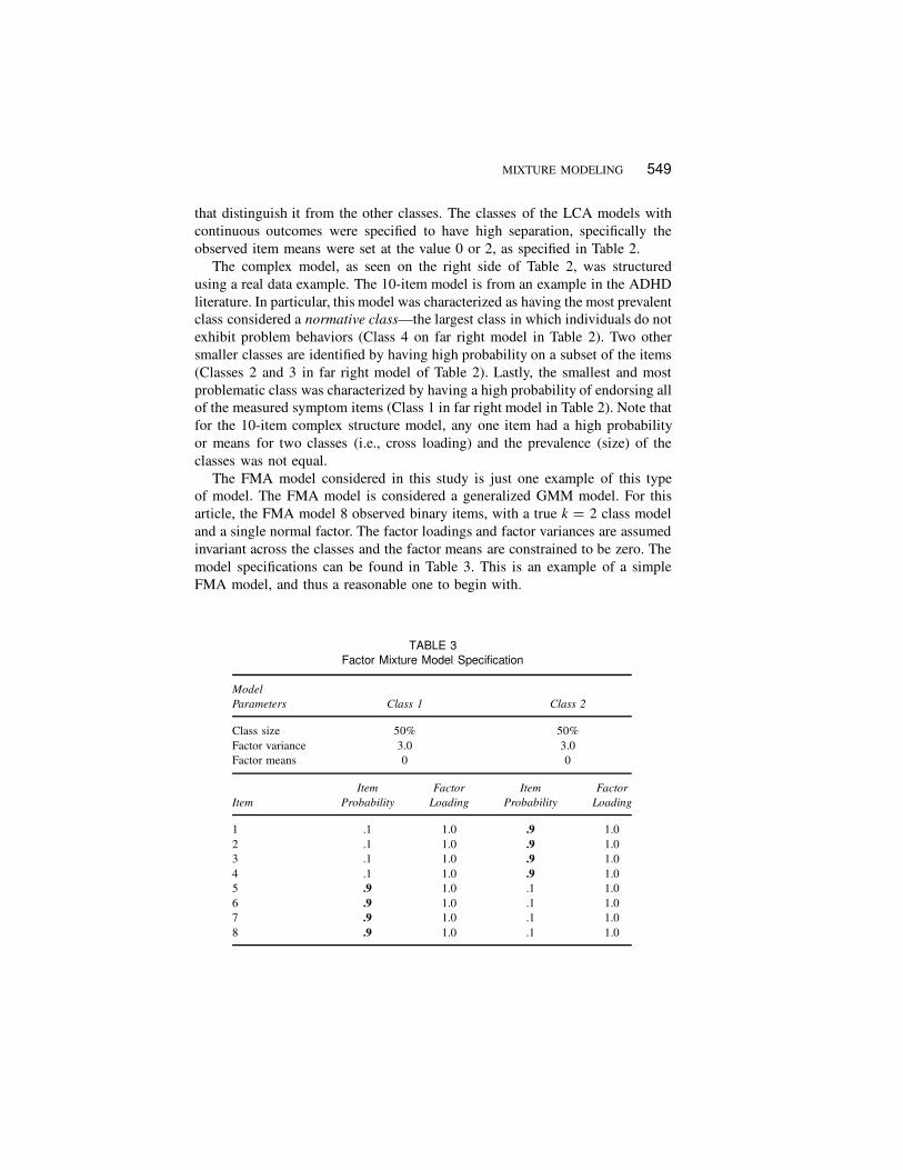
The FMA model considered in this study is just one example of this typeof model. The FMA model is considered a generalized GMM model. For thisarticle, the FMA model 8 observed binary items, with a true k D 2 class modeland a single normal factor. The factor loadings and factor variances are assumedinvariant across the classes and the factor means are constrained to be zero. Themodel specifications can be found in Table 3. This is an example of a simpleFMA model, and thus a reasonable one to begin with.

TABLE 3

Factor Mixture Model Specification

Model

Parameters Class 1 Class 2

Class size 50% 50%Factor variance 3.0 3.0Factor means 0 0

Item

Item

Probability

Factor

Loading

Item

Probability

Factor

Loading

1 .1 1.0 .9 1.02 .1 1.0 .9 1.03 .1 1.0 .9 1.04 .1 1.0 .9 1.05 .9 1.0 .1 1.06 .9 1.0 .1 1.07 .9 1.0 .1 1.08 .9 1.0 .1 1.0


TABLE 4

Growth Mixture Model Specification

Model Parameters

Class 1

Good Dev.

Class 2

Slow Dev.

Class size 75% 25%Growth parameters

Intercept mean 2.00 1.00Var(Intercept) 0.25 0.25Slope mean 0.50 0.00Var(Slope) 0.04 0.04Var(Intercept, Slope) 0.00 0.00

ResidualsVar(Y1) 0.15 0.15Var(Y2) 0.20 0.20Var(Y3) 0.20 0.20Var(Y4) 0.35 0.35

The GMM considered was a simple structure model. The GMM has a truek D 2 class model with continuous outcomes and has linear growth parameters.Specifically, as seen in Table 4, one class of the GMM is characterized as havinggood development where the mean of the intercept growth factor is 2.0 and themean slope factor is 0.5. This class is 75% of the sample. The second class,which is 25% of the sample, is characterized by having a lower intercept factormean (i.e., 1.0) and slope factor mean of zero. The separation of the mean initialvalue of the two classes in the GMM model is two, a value that is thought toprovide well-separated classes. The growth parameter and residual variances arespecified to be equal across the two classes.

For the GMM and FMA models, we specified a one- through four-classmodel and considered 100 replications. For these models, the performance ofthe likelihood-based tests and indexes may be more sensitive to the specificationof the alternative models. We specified alternative models to have similar modelattributes as the generated population model. Specifically, for the GMM models,we constrained the residual variances to be equal across classes, the covariancebetween the intercept and slope parameters were invariant across classes, andthe class prevalences were freely estimated. Further, for the alternative models,the slope and intercept means and variances were allowed to be class specific,where linear growth was assumed within each class.

Data Analysis Models

Data sets were generated according to the previously mentioned populationmodel attributes and were analyzed using a series of models that differed in


the number of classes. Each of the replications and the three different samplesizes were analyzed using two- through six-class analysis models. The LMRand BLRT p values are provided for each replication that converged.

The simulation and analysis of the sample data were conducted using theMonte Carlo facilities in Mplus Version 4.1 (L. Muthén & Muthén, 1998–2006).Within Mplus, the population and analysis models are easily specified and sum-mary information is provided across all completed replications. The LMR andBLRT p value can be obtained by specifying the output options of Tech 11 andTech 14, respectively. Nonconvergence of any given replication occurs becauseof the singularity of the information matrix or an inadmissible solution that wasapproached as a result of negative variances. As a result, model estimates andsummaries were not computed for these replications. This occurred in badlymisspecified models (e.g., where k D 3 in the data generation and the analy-sis specified a six-class model) and occurred less than 1% of the time for theLCA models, and at most 5% for the FMA and GMM models. In the FMA andGMM model setting, nonconvergence was considered an indication of modelmisfit, and was used as evidence that the model with one fewer classes wassuperior.

It is widely known that mixture models are susceptible to converging onlocal, rather than global, solutions. To avoid this, it is often recommended thatmultiple start values for estimated model parameters be considered (McLachlan& Peel, 2000). Observing the same log likelihood obtained from multiple setsof start values increases confidence that the solution obtained is not a localmaximum. Mplus Version 4 has a random start value feature that generates anumber of different random start sets, facilitating the exploration of possiblelocal solutions. Before moving on to the larger simulation study, a variety ofstart value specifications was considered to ensure that a sufficient number ofrandom starts were chosen to overcome local solutions.2 Thus, there is littlechance that the results of this study are based on local solutions. It should benoted that when using random start values in Mplus, the program goes throughthe random start value procedure for both the k �1 and the k class models whencalculating the LMR and BLRT p value.

One way to obtain the parametric BLRT p value is to generate and analyze,say, 500 replicated data sets and obtain a close approximation to the LRT distri-bution. This procedure, however, is computationally demanding. Typically, weneed to know only whether the p value is above or below 5%, as this would de-termine whether the LRT test would reject or accept the null hypothesis. Mplus

uses the sequential stopping rule approach described in the Appendix. When the

2The number random starts for LCA models with categorical outcomes was specified to be“starts D 70 7;” in Mplus. The models with continuous outcomes had differing numbers of randomstarts.


p value is close to 5%, this sequential procedure uses more replications thanwhen the p value is far from 5%.

In simulation studies, the analysis models must be able to accurately recoverthe population parameters. If the models chosen to analyze the simulated data arenot able to provide estimates that are close to the population parameters whencorrectly specified, results of the simulation have little meaning. For example,when four-class data are generated and analyzed with a four-class model, it isexpected that the estimated parameter values are close to the population param-eters that generated the data. The ability of the analysis models to recover thepopulation parameters can be summarized by looking at the number of replica-tions with confidence intervals that contain the true population parameter. Thesevalues are called coverage estimates and are considered for each one of theestimated parameters in the model. A coverage value of say, .93, for a given pa-rameter would indicate that, across all replications, 93% of the model estimatesfall within a 95% confidence interval of the population parameter value.3 Onerule of thumb is that coverage estimates for 95% confidence estimates shouldfall between .91 and .98 (L. Muthén & Muthén, 2002).

RESULTS

This section presents summaries from the simulation study. Results include in-formation on coverage, a comparison of the three likelihood-based tests (NCS,LMR, and BLRT), the performance of the ICs (AIC, CAIC, BIC, and adjustedBIC) in identifying the correct model, and the ability of the LMR and BLRT topick the correct model.

Coverage values for all the models (results are not presented here) werefound to be very good (between .92 and .98).4 The exceptions were in themodeling setting where there was a very small class (e.g., 5%). This occurs inthe complex, 10-item categorical LCA model with sample size n D 200 andthe 8-item categorical LCA with unequal classes with sample size n D 200. Inthis setting, the average coverage estimates for parameters in the smallest class(prevalence of 5%) were low (.54). These results were not surprising given thatclass size is only 10 (5% of 200). As sample size increases, coverage for thisclass increases in both settings to an average of .79 for n D 500 and .91 forn D 1,000.

3It is important to note that when coverage is studied, the random starts option of Mplus shouldnot be used. If it is used, label switching may occur, in that a class for one replication might berepresented by another class for another replication, therefore distorting the estimate.

4The models that presented convergence problems were those that were badly misspecified. Forexample, for the GMM (true k D 3 class model) for n D 500, the convergence rates for the three-,four-, and five-class models were 100%, 87%, and 68%, respectively.


Likelihood-Based Tests

Results comparing the three LRTs are presented in terms of their ability todiscriminate among neighboring class models. By neighboring class models, weare referring to models that differ by one class from the true population model.Thus, we focus on the performance of the LRTs by looking at the rate at whichthe indexes are able to discriminate between both the k �1 versus k class modelsand the k versus kC1 class models, where k is the correct number of classes. Wenarrow our focus in this way because we assume that a very misspecified model(e.g., one where we specify a two-class model and the population is a six-classmodel) would be easily identified by these tests. We are more concerned withthe ability to reject models that are close to the true population model. Generallyspeaking, both the LMR and the BLRT methods are able to distinguish betweenthe k � g and k lass models (where g < k), which is how they are commonlyused in practical applications.

Type I Error Comparison

Table 5 contains information on the Type I error rates for the LRTs considered(NCS, LMR, and BLRT). This information concerns the ability of the tests to“correctly” identify the k class model in comparison to the k C 1 class model.Table 5 gives the estimated Type I error (i.e., the probability of incorrectlyrejecting a true model). If these tests worked perfectly, in that they correctlyidentified the k class model, we would expect the values in the cells to beapproximately .05. The values in this table can be thought of as error rates.For example, looking at the 8-item categorical LCA model column for n D

200, we observe that the LMR’s proportion rejected is .25. This means thatfor 25% of the replications for n D 200, the LMR incorrectly rejects the nullfour-class model in favor of the alternative five-class model. Knowing that thetrue population model has k D 4 classes for the 8-item model, we would notwant to reject the null and hope that the overall rejection proportion would bearound .05.

Looking at Table 5, we first notice that the NCS has an inflated Type Ierror rate across nearly all modeling settings. This is evident by noting that theerror rates are consistently higher than the expected value of .05. The LMR hasinflated Type I error rates for the LCA models with categorical outcomes andfor the FMA and GMM models, but has adequate Type I error rates for theLCA with continuous outcomes. The BLRT works remarkably well, where weobserve Type I error rates near or below .05 for all model structure and samplesize combinations. When comparing the performance across LCA models forall sample sizes, the LMR consistently outperforms the NCS, and the BLRToutperforms both the NCS and LMR.


TABLE 5

Type I Error Rates for the Three Likelihood Ratio Tests: NCS, LMR, and BLRT

8-Item Simple Structure

15-Item

Simple Structure

10-Item

Complex Structure

Equal Classes Unequal Classes Equal Classes Unequal Classes

H0: 4-Class (True) H0: 4-Class (True) H0: 3-Class (True) H0: 4-Class (True)

H1: 5-Class H1: 5-Class H1: 4-Class H1: 5-Class

n NCS LMR BLRT NCS LMR BLRT NCS LMR BLRT NCS LMR BLRT

Latent class analysis with categorical outcomes

200 .33 .25 .05 .30 .11 .04 .97 .10 .08 .51 .17 .06500 .41 .25 .04 .36 .19 .07 .98 .07 .05 .66 .19 .06

1,000 .48 .18 .05 .41 .12 .05 .99 .06 .05 .73 .21 .06

Latent class analysis with continuous outcomes

200 .74 .11 .06 .60 .02 .04 .56 .03 .04500 .76 .06 .03 .62 .06 .01 .47 .03 .03

1,000 .79 .06 .02 .75 .03 .02 .49 .02 .04

Other Mixture Models

FMA 8-Item

Binary Outcome

GMM 4 Time-Point,

Linear Growth

H0: 2-Class (True) H0: 2-Class (True)

H1: 3-Class H1: 3-Class

n NCS LMR BLRT NCS LMR BLRT

200 .48 .22 .10 .11 .07 .05500 .49 .19 .08 .16 .12 .06

1,000 .51 .21 .07 .08 .16 .01

Note. NCS D naive chi-square; LMR D Lo–Mendell–Rubin; BLRT D bootstrap likelihoodratio test; FMA D factor mixture model; GMM D growth mixture model.

Focusing solely on the values in the NCS column, we notice that the error rateincreases as sample size increases, which could be caused by known problems ofthe chi-square statistic when analyzing large samples. Comparing the similarlystructured 8- and 15-item models for both continuous and categorical outcomemodels, the LMR performs better in LCA models with more items. Lookingacross the categorical LCA model results, both the NCS and BLRT performbest for the model with fewest items, the 8-item simple structure model. TheGMM results show the LMR performs about the same as NCS, but the BLRTis the clear winner. Note that for GMMs, the LMR Type I error rate increasesas sample size increases, a pattern not seen in other modeling settings. For theFMA model, the BLRT is the clear winner over the other tests. Overall, the


BLRT performs very well in terms of Type I error (e.g., all values are close to.05) across all model settings.

Power Comparisons

Table 6 is concerned with power (i.e., the probability that the test will rejectthe null hypothesis when it is false). Thus, values of at least .80 would indicatethat the particular test worked well in finding the true k class model. Table 6summarizes testing the k � 1 class model against the correct k class model. Incontrast to the discussion of Type I error in Table 5, in this setting we wantthe null hypothesis to be rejected in favor of the alternative. It is meaningfulto compare the power across approaches only when their Type I error rate is at

TABLE 6

Power Values for the Three Likelihood Ratio Tests: NCS, LMR, and BLRT

8-Item Simple Structure

15-Item

Simple Structure

10-Item

Complex Structure

Equal Classes Unequal Classes Equal Classes Unequal Classes

H0: 3-Class H0: 3-Class H0: 2-Class H0: 3-Class

H1: 4-Class (True) H1: 4-Class (True) H1: 3-Class (True) H1: 4-Class (True)

n NCS LMR BLRT NCS LMR BLRT NCS LMR BLRT NCS LMR BLRT

Latent class analysis with categorical outcomes

200 1.00 .95 1.00 .80 .36 .53 .97 1.00 1.00 .98 .62 .84500 1.00 1.00 1.00 .98 .75 .94 .98 1.00 1.00 1.00 .90 1.00

1,000 1.00 1.00 1.00 1.00 .96 1.00 .99 1.00 1.00 1.00 .98 1.00

Latent class analysis with continuous outcomes

200 1.00 1.00 1.00 .99 1.00 1.00 1.00 .67 .98500 1.00 1.00 1.00 1.00 1.00 1.00 1.00 1.00 1.00

1,000 1.00 1.00 1.00 1.00 1.00 1.00 1.00 1.00 1.00

Other Mixture Models

FMA 8-Item

Binary Outcome

GMM 4 Time-Point,

Linear Growth

H0: 1-Class H0: 1-Class

H1: 2-Class (True) H1: 2-Class (True)

n NCS LMR BLRT NCS LMR BLRT

200 1.00 1.00 1.00 1.00 .85 .95500 1.00 1.00 1.00 1.00 1.00 1.00

1,000 1.00 1.00 1.00 1.00 1.00 1.00

Note. NCS D naive chi-square; LMR D Lo–Mendell–Rubin; BLRT D bootstrap likelihoodratio test; FMA D factor mixture model; GMM D growth mixture model.


an acceptable rate. Because the Type I error rates for the NCS are consistentlyinflated (e.g., well above .05), it does not make sense to compare power rates forthis test. Thus, we consider only the LMR and BLRT for the power comparisons.The LMR, however, does have inflated Type I error in certain settings.

Table 6 shows that for both the LMR and BLRT, there is sufficient power todetect the k class model in almost all of the models. The exceptions are for theLMR where the power is .36 for the categorical LCA with 8 items with unequalclass sizes and is .62 for the 10-item LCA, n D 200 modeling with categoricaloutcomes, and .67 for the 10-item LCA, n D 200 modeling with continuousoutcomes. The only setting where BLRT has lower than expected power is inthe 8-item categorical LCA setting with n D 200 where there is a power of .53.The power quickly reaches an acceptable value as the sample size increases.Even in the 10-class modeling setting with small sample size, the BLRT hassufficient power. The LMR power is low for the GMM, but there are also highType I error rates so power results are not meaningful.

Information Criteria

The likelihood-based results presented in Tables 5 and 6 are concerned withcomparing neighboring class models. For the ICs, we compare values across aseries of model specifications. The values in Table 7 were computed by com-paring the AIC, CAIC, BIC, and adjusted BIC across all models (two- throughsix-class models), then identifying where the lowest values occurred across thosemodels considered. For example, looking at the 8-item LCA model with cate-gorical outcomes (which is a true four-class model) we note that for n D 500,the lowest values of AIC occurred at the four-class model 68% of the time and100% of the time for CAIC, BIC, and adjusted BIC. A value of 100 in the boldedcolumn indicates perfect identification of the k class model by one of the indexes.

Looking across all the models considered there are a few general trends worthnoting. First, the AIC does not seem to be a good indicator for identifying thek class model for any of the modeling settings. The value in the bolded columnindicates that, at best, the AIC correctly identifies the k class model 75% ofthe time when looking across all models and sample size considerations. Also,notice that accuracy decreases as sample size increases, a known problem withAIC because there is no adjustment for sample size. Further, we notice thatwhen AIC is not able to identify the correct k class model, it is most likelyto identify the k C 1 class model as the correct model. The CAIC is able tocorrectly identify the correct k class model close to 100% of the time for boththe 8- and 15-item categorical LCA models and for most of the continuous itemLCA, regardless of sample size, and performs well for both the FMA and GMMmodels, regardless of sample size. For the categorical 10-item, complex model,the CAIC performance was much worse, identifying the correct model only 1%


TABLE 7

Percentage of Times the Lowest Value Occurred in Each Class Model

for the AIC, CAIC, BIC, and Adjusted BIC

Latent Class Analysis with Categorical Outcomes

AIC CAIC BIC Adjusted BIC

Classes Classes Classes Classes

Model n 2 3 4 5 6 2 3 4 5 6 2 3 4 5 6 2 3 4 5 6

8-item(Simple,Equal)

200 0 0 75 22 3 0 5 95 0 0 0 1 99 0 0 0 0 83 15 2500 0 0 68 27 5 0 0 100 0 0 0 0 100 0 0 0 0 100 0 0

1000 0 0 60 32 8 0 0 100 0 0 0 0 100 0 0 0 0 100 0 0


n 2 3 4 5 6 2 3 4 5 6 2 3 4 5 6 2 3 4 5 6

8-item(Simple,Unequal)

200 0 26 48 24 2 83 17 0 0 0 58 42 0 0 0 0 29 58 12 1500 0 2 67 27 4 6 83 11 0 0 1 72 27 0 0 0 12 88 0 0

1000 0 0 62 33 5 0 26 74 0 0 0 12 88 0 0 0 0 100 0 0


n 2 3 4 5 6 2 3 4 5 6 2 3 4 5 6 2 3 4 5 6


200 0 43 41 13 3 0 100 0 0 0 0 100 0 0 0 0 62 31 6 1500 0 32 41 17 6 0 100 0 0 0 0 100 0 0 0 0 99 1 0 0

1000 0 31 45 17 6 0 100 0 0 0 0 100 0 0 0 0 100 0 0 0


n 2 3 4 5 6 2 3 4 5 6 2 3 4 5 6 2 3 4 5 6

10-item(Complex,Unequal)

200 0 5 67 24 3 2 97 1 0 0 0 92 8 0 0 0 7 76 15 2500 0 0 55 35 9 0 44 56 0 0 0 24 76 0 0 0 1 98 1 0

1000 0 0 46 39 14 0 1 99 0 0 0 0 100 0 0 0 0 100 0 0

(continued )

and 56% of the time for n D 200 and n D 500, respectively. For the larger samplesize of n D 1,000, the CAIC performed well. The CAIC’s adjustment for thenumber of parameters using sample size significantly improves its performanceover the AIC.

The BIC and the adjusted BIC are comparatively better indicators of thenumber of classes than the AIC. Both the BIC and adjusted BIC are sample sizeadjusted and show improvement at identifying the true k class model as samplesize increases. The BIC correctly identified the k class model close to 100% ofthe time for both the categorical and continuous 15-item and 8-item LCA modelswith equal class size. In the 10-item categorical LCA model with unequal classsize, it only identified the correct model 8% of the time when n D 200 and for


TABLE 7

(Continued )

Latent Class Analysis with Continuous Outcomes



Model n 2 3 4 5 6 2 3 4 5 6 2 3 4 5 6 2 3 4 5 6

8-item(SimpleStructure)

200 0 0 33 35 32 0 0 100 0 0 0 0 100 0 0 0 0 49 31 20500 0 0 42 34 24 0 0 100 0 0 0 0 100 0 0 0 0 95 5 0

1000 0 0 29 43 28 0 0 100 0 0 0 0 100 0 0 0 0 100 0 0


n 2 3 4 5 6 2 3 4 5 6 2 3 4 5 6 2 3 4 5 6


200 1 39 44 16 0 1 99 0 0 0 1 99 0 0 0 1 58 32 9 0500 0 42 39 17 2 0 99 0 1 0 0 99 0 1 0 0 99 0 1 0

1000 0 29 39 21 11 0 100 0 0 0 0 100 0 0 0 0 100 0 0 0


n 2 3 4 5 6 2 3 4 5 6 2 3 4 5 6 2 3 4 5 6

10-item(ComplexStructure)

200 0 0 65 21 14 0 35 65 0 0 0 26 74 0 0 0 0 75 18 7500 0 0 59 30 11 0 0 100 0 0 0 0 100 0 0 0 0 99 1 0

1000 0 0 68 23 9 0 0 100 0 0 0 0 100 0 0 0 0 100 0 0

Factor Mixture Model with Categorical Outcomes



Model n 1 2 3 4 1 2 3 4 1 2 3 4 1 2 3 4

FMA 200 0 59 33 8 0 94 6 0 0 100 0 0 0 69 27 4500 0 59 27 14 0 100 0 0 0 100 0 0 0 97 3 0

1000 0 58 28 14 0 100 0 0 0 100 0 0 0 94 3 3

Growth Mixture Model with Continuous Outcomes



Model n 1 2 3 4 1 2 3 4 1 2 3 4 1 2 3 4

GMM 200 0 58 22 20 0 98 2 0 16 84 0 0 0 66 18 16500 0 65 24 11 0 100 0 0 0 100 0 0 0 90 9 1

1000 0 64 24 12 0 100 0 0 0 100 0 0 0 100 0 0

Note. Columns in boldface type represent the true k-class for the given model. AIC D Akaike’s InformationCriterion; CAIC D Consistent Akaike’s Information Criterion; BIC D Bayesian Information Criterion.


the categorical 8-item LCA with unequal class size, it was never able to identifythe correct model for n D 200. For the 10-item categorical LCA, performanceincreased as n increased, reaching 100% correct identification when n D 1,000.For the categorical 8-item LCA with unequal class size, the performance ofthe BIC increases as sample size increases, eventually reaching 88% for n D

1,000. The BIC identified the correct model 74% of the time for the 10-itemcontinuous LCA model, n D 200, and jumped to 100% for n D 500. In both theFMA and GMM modeling settings, BIC performed well across all sample sizes.The adjusted BIC performs relatively well across all models, but shows someweakness when the sample size is small. For n D 200 in the categorical LCA15- and 10-item models, adjusted BIC correctly identified the k class model only62% and 76% of the time, respectively. In general, when the adjusted BIC goeswrong, it tends to overestimate the number of classes. In summary, comparingacross all the models and sample sizes, there seems to be strong evidence thatthe BIC is the best of the ICs considered.

Likelihood-Based Tests

Table 8 contains information on the performance of the three likelihood-basedtests: the NCS, LMR, and BLRT. Similar to the results presented in Table 7,these results are based on comparing across different numbers of classes for aset of models. To calculate these values, we examined the p values resultingfrom specifying the two- through six-class models for each replication. Notethat for these LMR and BLRT, when specifying a two-class model, we comparethe one-class model to the two-class model. Note that we specified alternativemodels that range between two and six classes. Thus, for Table 8 the possiblesolution for the LMR and BLRT ranges from a one-class model to a five-class model for the LCA models, and range from one class to three classesfor the FMA and GMM models. For the NCS, we obtain p values using thetraditional chi-square distribution. The p value provided is used to assess ifthere is significant improvement between the specified model and a model withone less class. Looking at these p values, we identified the model selected basedon the occurrence of the first nonsignificant p value (p > .05). A bolded valueclose to .95 would indicate that the test performed close to perfectly. The boldednumber in the LMR column in the categorical LCA eight-class model for n D

500 indicates that 78% of the replications concluded that the correct four-classsolution was the correct model.

Results in Table 8 indicate a clear advantage of the BLRT over the NCS andLMR. In almost all LCA model and sample size considerations, the BLRT isable to correctly identify the true k class model nearly 95% of the time. Lookingat the NCS and considering the LCA models, we notice that the performancedecreases as sample size increases and remains consistently poor. For the FMA


TABLE 8

Percentage of Time a Nonsignificant p Value Selected the Given Class Model

for the NCS, LMR, and BLRT

Latent Class Analysis with Categorical Outcomes

NCS LMR BLRT

Classes Classes Classes

Model n 1 2 3 4 5 6 1 2 3 4 5 1 2 3 4 5


200 0 0 0 67 29 4 4 8 6 64 18 0 0 0 96 4500 0 0 0 58 33 9 0 0 0 78 22 0 0 0 96 5

1000 0 0 0 52 36 13 0 0 0 83 17 0 0 0 95 5


n 1 2 3 4 5 6 1 2 3 4 5 1 2 3 4 5

8-item(Simple,Unequal)

200 0 0 20 50 26 4 6 30 39 21 4 0 0 47 49 4500 0 0 1 62 28 9 0 10 23 53 10 0 0 6 87 7

1000 0 0 0 60 31 9 0 7 4 78 11 0 0 0 95 5


n 1 2 3 4 5 6 1 2 3 4 5 1 2 3 4 5


200 0 0 3 29 40 29 0 0 90 9 1 0 0 92 7 1500 0 0 2 19 34 45 0 0 93 6 1 0 0 95 5 0

1000 0 0 1 17 31 50 0 0 94 6 0 0 0 95 5 0


n 1 2 3 4 5 6 1 2 3 4 5 1 2 3 4 5

10-item(Complex,Unequal)

200 0 0 2 48 41 10 5 9 34 43 9 0 0 16 78 6500 0 0 0 34 45 21 1 4 9 72 14 0 0 0 94 6

1000 0 0 0 26 41 33 0 2 2 80 17 0 0 0 94 6

(continued )

model, the NCS performs consistently poorly, specifically identifying the correctmodel only about 60% of the time across all sample sizes. For the GMM model,however, the NCS performed consistently well, although not as well as theBLRT. In the categorical LCA 15-item models, the LMR performs almost aswell as the BLRT, where between 90% and 94% of the time the LMR picked thecorrect number of classes. In this same setting, the NCS performs very poorly,identifying the correct model, at most, only 3% of the time. For LCA modelswith continuous outcomes, the LMR and BLRT perform very well for n D 500and 1,000. For both the categorical and continuous LCA, in the 15-item models,the LMR performs rather well, where it identifies the correct model over 90%of the time for all sample sizes.


TABLE 8

(Continued )

Latent Class Analysis with Continuous Outcomes

NCS LMR BLRT


Model n 1 2 3 4 5 6 1 2 3 4 5 1 2 3 4 5


200 0 0 0 26 37 37 0 5 0 84 9 0 0 0 94 6500 0 0 0 24 36 40 0 0 0 94 5 0 0 0 97 3

1000 0 0 0 21 44 35 0 0 0 94 5 0 0 0 98 2


n 1 2 3 4 5 6 1 2 3 4 5 1 2 3 4 5


200 0 1 39 41 17 2 0 0 98 2 0 0 0 96 3 1500 0 0 38 44 18 0 0 0 94 6 0 0 0 99 1 0

1000 0 0 25 49 21 5 0 0 97 3 0 0 0 98 2 0


n 1 2 3 4 5 6 1 2 3 4 5 1 2 3 4 5

10-item(ComplexStructure)

200 0 0 0 56 34 10 0 21 30 48 1 0 0 2 94 3500 0 0 0 46 36 18 0 5 0 93 1 0 0 0 97 3

1000 0 0 0 49 34 17 0 4 0 94 2 0 0 0 96 3

Factor Mixture Model

with Categorical Outcomes

NCS LMR BLRT


Model n 1 2 3 4 1 2 3 1 2 3

FMA 200 0 60 40 0 0 80 20 0 87 13500 0 61 39 0 0 84 16 0 92 8

1000 0 60 40 0 0 84 16 0 93 7

Growth Mixture Model

with Continuous Outcomes

NCS LMR BLRT


Model n 1 2 3 4 1 2 3 1 2 3

GMM 200 0 90 10 0 14 81 5 5 90 5500 0 84 14 2 0 90 10 0 94 6

1000 0 92 8 0 0 85 15 0 99 1

Note. NCS D naive chi-square; LMR D Lo–Mendell–Rubin; BLRT D bootstrap likelihood ratio test.


DISCUSSION AND CONCLUSIONS

This simulation considered the performance of the three likelihood-based tests(NCS, LMR, and BLRT) and commonly used fit indexes used for determiningthe number of classes in mixture models with both categorical and continuousoutcomes. We set out to understand how misleading it would be if the NCStest was used for these models compared to the newly proposed LMR and theBLRT. We also considered the conventional IC indexes.

Comparing the Likelihood-Based Tests

The results of this study support the fact that a researcher using the NCS fortesting the k �1 versus k class model would reject the true model too frequently.It is noted that the NCS is especially sensitive to sample size, and its performanceactually worsens as sample size increases for LCA models. As mentioned before,we know that this test is not appropriate for testing nested mixture models. Itcould be that this assumption violation is amplified as sample size is increased.It is important to note that, as seen in Table 8, when the NCS goes wrong, ittends to overestimate the number of classes. As an alternative to the NCS, theother LRTs, the LMR and BLRT, were shown to have the ability to identifythe correct model more accurately. The BLRT clearly performed better than theLMR in almost all modeling settings.

We consider only the power results for the LMR and BLRT because there arehigh Type I error rates for the NCS test. There is good power for both the LMRand BLRT for nearly all the models considered in this study. The BLRT hasmore consistent power across all sample sizes than the LMR. Slight differencesin power across the BLRT and LMR do not indicate a significant distinctionin performance between the two tests in terms of power (i.e., distinguishingbetween the k and k � 1 class models).

Considering the LMR results in Table 8, we notice that, in general, for LCAmodels if the LMR incorrectly identifies a model, it tends to overestimate thenumber of classes. Thus, to the analyst using the LMR as a tool for classenumeration, when the p value indicates a nonsignificant difference for the LMR,one can feel somewhat confident that there is, at most, that number of classes,but that there might, in fact, be fewer. Overestimating the number of classescan be thought of as being better than underidentifying classes, as the true k

class solution can still be extracted from a k C 1 class solution. For example, ifthe true solution is k D 3 and the model LMR identified a four-class solution,it could be the case that one of the classes in the four-class solution does notmake substantive sense or there is a very small class that is hard to identify.This could result in the decision to not go with the four-class solution despitethe LMR results, and instead settle on the true three-class solution. If LMR had


indicated that a two-class model was most fitting, it might be more difficult tosomehow increase the number of classes and settle on the true k D 3 classmodel.

For LCA models, the BLRT has better accuracy for correctly identifyingthe true number of classes. The only setting in which the BLRT has a correctidentification rate below 92% is in the categorical LCA 10-item setting whenn D 200. As noted before, this was a difficult modeling setting, where there wasone small class with very few observations. Further, for the LCA models withcontinuous outcomes, FMA and GMM models, the BLRT performs the best outof the likelihood tests presented.

As mentioned previously, both the LMR test and BLRT provide a p value thatcan be used to decide whether the k � 1-class model should be rejected in favorof the k class model. In practice, for a researcher fitting a series of LCA models,the LMR may result in p values that bounce around from being significant tononsignificant and then back to significant again. This does not appear to be thecase for the p value based on the BLRT. Findings show that once the BLRT p

value is nonsignificant, it remains nonsignificant for the subsequent increasedclass models. Based on experience and the findings of this study, preliminaryresults suggest the first time the p value of the LMR is nonsignificant might bea good indication to stop increasing the number of classes.

Comparing the Information Criteria

Summary information for the AIC, CAIC, BIC, and adjusted BIC were includedto aid in understanding the utility of these indexes in LCA and GMM modelingsettings. The results are in agreement with previous research indicating the AICis not a good indicator for class enumeration for LCA models with categoricaloutcomes (Yang, 2006). Based on the results, the AIC is not a good indicatorof class for any of the models considered in this study. The CAIC showed aclear improvement over the AIC in both categorical and continuous LCA, butwas sensitive to the combination of unequal class sizes and a small sample sizefor LCA models with categorical outcomes. The CAIC is not widely used forclass enumeration, and more studies should look at its performance given itsclear superiority to AIC in certain modeling situations.

Based on the results of this study, when comparing across all modeling set-tings, we conclude that the BIC is superior to all other ICs. For categorical LCAmodels, the adjusted BIC correctly identifies the number of classes more consis-tently across all models and all sample sizes. In this setting, the BIC performedwell for the 8- and 15-item categorical LCA models with equal class sizes, butperformance decreased for the two categorical LCA models with unequal classsize (e.g., the 10-item, complex structure with unequal class size and the 8-item,simple structure with unequal class size). When considering continuous LCA,


however, the superiority of the BIC is more evident. The BIC more consistentlyidentifies the correct model over the adjusted BIC, where the adjusted BIC dropsas low as 49% for the 8-item model with n D 200. For both the FMA and GMM,the BIC performs well, where at worst it identifies the correct model 84% ofthe time. Based on these results, we conclude that the BIC is the most consis-tent IC among those considered for correctly identifying the number of classes.Table 7 shows that the BIC has sensitivity to small sample sizes, regardless ofthe type of model. Undoubtedly, there needs to be further study to facilitatea greater understanding of the impact of the structure on the performance ofthese ICs.

Comparing the BIC and BLRT

We can compare the results of Tables 7 and 8 to understand the performance ofthe BIC, the best performing of the ICs, to the BLRT, the best performing of theLRTs. For the LCA with categorical outcomes, the BLRT is more consistent atidentifying the correct number of classes than the BIC, because at its worst, theBLRT identifies the correct number of classes 49% of the time. This is betterthan the BIC, which at its worst, is not able to identify the correct numberof classes at all for the 8-item categorical outcome LCA model with unequalclasses, n D 200. Considering the LCA with continuous outcomes, the BICperforms well, but it correctly identifies the correct model only 74% of the timefor n D 200. In this setting, the BLRT is consistent; it identifies the correctmodel a remarkable 94% of the time. Comparing the results of Tables 7 and 8for the FMA and GMM models, both the BIC and BLRT perform well. In thissetting, BIC, at its worst, identifies the correct model 84% of the time for theGMM where n D 200; at its worst, the BLRT identifies the correct model 87%of the time for the FMA with n D 200. Thus, considering all the models inthis study, the BLRT stands out as the most consistent indicator for the correctnumber of classes when comparing results from Tables 7 and 8.

Although the results presented here represent only a small subset of all mix-ture models, it is important to note that the FMA and GMM results are based ononly one model of each. Thus, when comparing the results presented in Tables 7and 8, the FMA and GMM results are not given as much weight as the LCAmodels. A recent simulation study by Tofighi and Enders (2006) more closelyexamines class enumeration issues for a wider range of GMM models.

In summary, the results of this study indicate a clear advantage of the BLRTtest compared to NCS and LMR, and show that it can be used as a reliable toolfor determining the number of classes for LCA models. The BIC was found tocorrectly identify the number of classes better than the other ICs considered, forLCA models and FMA and GMM models. The LMR performed better than theNCS, but not as well as the BLRT. If one had to choose one of the IC indexes,


the BIC would be the tool that seems to be the best indicator of the number ofclasses. The BLRT would be chosen over the LMR because of its consistency inchoosing the correct class model. Overall, by comparing the results in Tables 7and 8 across all models and sample sizes, the BLRT is the statistical tool thatperforms the best of all the indexes and tests considered for this article.

The BLRT, however, does have its disadvantages. It should be noted thatwhen using the BLRT, the computation time increased 5 to 35 times in ourexamples. Another disadvantage of the BLRT approach is that it depends ondistributional and model assumptions. The replicated data sets are generatedfrom the estimated model and have the exact distributions as the ones used inthe model. Thus, if there is a misspecification in the model or the distributions ofthe variables, the replicated data sets will not be similar in nature to the originaldata set, which leads to incorrect p value estimation. For example, if data within aclass are skewed but modeled as normal, the BLRT p value might be incorrect.Outliers can also lead to incorrect p value estimates. In addition, the BLRTcannot currently accommodate complex survey data. Similarly, the various ICsdepend on the model, distributional and sampling assumptions. On the otherhand, the LMR is based on the variance of the parameter estimates, which arerobust and valid under a variety of model and distributional assumptions andcan accommodate complex survey data. Thus, the LMR may be preferable insuch contexts. Our simulations, however, did not evaluate the robustness of thetests and more research on this topic is needed.

Recommendations for Practice

Due to the increased amount of computing time of the BLRT, it might be better tonot request the BLRT in the initial steps of model exploration. Instead, one coulduse the BIC and the LMR p values as guides to get close to possible solutionsand then once a few plausible models have been identified, reanalyze thesemodels requesting the BLRT. Further, although it is known that the likelihoodvalue cannot be used to do standard difference testing, the actual value of thelikelihood can be used as an exploratory diagnostic tool to help decide on thenumber of classes in the following way.

Figure 5 displays four plots of log likelihood values for models with differ-ing numbers of classes that can be used as a descriptive for deciding on thenumber of classes. Looking at the upper left panel, the 8-item LCA with cate-gorical outcomes (n D 1,000), we see a pattern of the likelihood increasing bya substantial amount when moving from two classes to three classes, and alsowhen we move from three classes to four classes. Then there is a flattening outwhen moving from four classes to five classes and similarly when moving fromfive classes to six classes. The flattening out of the lines between four and fiveclasses suggests that there is a nonsubstantial increase in the likelihood when


you increase from four to five. In addition, we observed a flattening out thathappens at the correct point for the 8-item model because we know that it is atrue k D 4 class model. We see a similar pattern for almost all modeling settings.The 10-item, n D 200 model does not have as dramatic of a flattening out asthe others, but as discussed before this is the most difficult modeling setting.This is also observed for the GMM model plot. Although there are only fourplots included, the general findings suggest that the log likelihood plot fairlyconsistently identifies the correct model for the LCA models with n D 500

and n D 1,000. Although we know we cannot test these log likelihood valuesfor difference testing using conventional methods, this plot is a way to use thelikelihoods as a descriptive tool when exploring the number of classes.

It is important to note that the selection of models for this study did notallow conclusions to be made about the specific model and sample attributes’impact on the results. For example, we do not generalize about the performanceof these tests and indexes for a particular type model structure, like the simplestructure model. Rather, model and sample selection were motivated by want-ing to explore a range of mixture models to understand the performance ofthe LRTs and the ICs. Future studies could aim to better understand the per-formance of the indexes for class enumeration and interrelation between thestructure of the models, nature of the outcomes (categorical vs. continuous), andnumber of items.

CONCLUSIONS AND FUTURE DIRECTIONS

This study explored the performance of IC and likelihood-based tests to identifythe correct number of classes in mixture modeling. Among the tools consideredin this study, results indicated that the BLRT outperformed the others. Secondbest was the BIC, followed by the adjusted BIC. Although previous researchhas looked at a variety of fit indexes and tests for deciding on the number ofclasses, this article is one of the first to closely examine the performance of theBLRT method for these types of mixture models. By considering LCA modelswith both categorical and continuous outcomes as well as a limited number ofFMA and GMM models, we expand the understanding of the performance of theICs and likelihood-based tests beyond what has been examined before. Theseresults, however, are merely a preview. More studies looking at the BLRT andits performance over a wider range of LCA models (e.g., including covariates,differently structured models, and the combination of continuous and categoricaloutcomes) should be considered before broad statements about its utility aremade. Nevertheless, these results contribute to a further understanding of howto decide on the number of classes in mixture models by providing more insightinto the performance of these indicators.


ACKNOWLEDGMENTS

Karen L. Nylund’s research was supported by Grant R01 DA11796 from theNational Institute on Drug Abuse (NIDA) and Bengt O. Muthén’s research wassupported by Grant K02 AA 00230 from the National Institute on Alcohol Abuseand Alcoholism (NIAAA). We thank Mplus for software support, Jacob Cheadlefor programming expertise, and Katherine Masyn for helpful comments.

REFERENCES

Akaike, H. (1987). Factor analysis and AIC. Psychometrika, 52, 317–332.Bollen, K. (1989). Structural equations with latent variables. New York: Wiley.Bozdogan, H. (1987). Model selection and Akaike’s information criterion (AIC): The general theory

and its analytical extensions. Psychometrika, 52, 345–370.Bucholz, K., Hesselbrock, V., Heath, A., Kramer, J., & Schuckit, M. (2000). A latent class analysis

of antisocial personality disorder symptom data from a multi-centre family study of alcoholism.

Addiction, 95, 553–567.Celeux, G., & Soromenho, G. (1996). An entropy criterion for assessing the number of clusters in

a mixture model. Journal of Classification, 13, 195–212.Collins, L. M., Fidler, P. L., Wugalter, S. E., & Long, J. D. (1993). Goodness-of-fit testing for latent

class models. Multivariate Behavioral Research, 28, 375–389.Formann, A. K. (2003). Latent class model diagnostics-A review and some proposals. Computational

Statistics & Data Analysis, 41, 549–559.Garrett, E. S., & Zeger, S. L. (2000). Latent class model diagnosis. Biometrics, 56, 1055–1067.Greenbaum, P., Del Boca, F., Darkes, J., Wang, C.-P., & Goldman, M. (2005). Variation in the

drinking trajectories of freshmen college students. Journal of Consulting and Clinical Psychology,

73, 229–238.Hagenaars, J., & McCutcheon, A. (Eds.). (2002). Applied latent class analysis models. New York:

Cambridge University Press.Jedidi, K., Jagpal, H., & DeSarbo W. S. (1997). Finite-mixture structural equation models for

response-based segmentation and unobserved heterogeneity. Marketing Science, 16, 39–59.Jeffries, N. (2003). A note on “Testing the number of components in a normal mixture.” Biometrika,

90, 991–994.Keel, P., Fichter, M., Quadflieg, N., Bulik, C., Baxter, M., Thornton, L., et al. (2004). Application

of a latent class analysis to empirically define eating disorder phenotypes. Archives of General

Psychiatry, 61, 192–200.Lazarsfeld, P., & Henry, N. (1968). Latent structure analysis. New York: Houghton-Mifflin.Li, F., Duncan, T., Duncan, S., & Hops, H. (2001). Piecewise growth mixture modeling of adolescent

alcohol use data. Structural Equation Modeling, 8, 175–204.Lo, Y., Mendell, N., & Rubin, D. (2001). Testing the number of components in a normal mixture.

Biometrika, 88, 767–778.Lubke, G. H., & Muthén, B. (2005). Investigating population heterogeneity with factor mixture

models. Psychological Methods, 10, 21–39.Magidson, J., & Vermunt, J. (2004). Latent class models. In D. Kaplan (Ed.), Handbook of quanti-

tative methodology for the social sciences (pp. 175–198). Newbury Park, CA: Sage.McCutcheon, A. C. (1987). Latent class analysis. Beverly Hills, CA: Sage.McLachlan, G., & Peel, D. (2000). Finite mixture models. New York: Wiley.


Muthén, B. (2004). Latent variable analysis: Growth mixture modeling and related techniques forlongitudinal data. In D. Kaplan (Ed.), Handbook of quantitative methodology for the social

sciences (pp. 345–368). Newbury Park, CA: Sage.Muthén, B. (2006). Should substance use disorders be considered as categorical or dimensional?

Addiction, 101(Suppl. 1), 6–16.Muthén, B., & Asparouhov, T. (2006). Item response mixture modeling: Application to tobacco

dependence criteria. Addictive Behaviors, 31, 1050–1066.Muthén, B., & Asparouhov, T. (2007). Growth mixture analysis: Models with non-Gaussian random

effects. Forthcoming in Fitzmaurice, G., Davidian, M., Verbeke, G., & Molenberghs, G. (eds.),Advances in Longitudinal Data Analysis. Chapman & Hall/CRC Press.

Muthén, B., Asparouhov, T., & Rebollo, I. (2006). Advances in behavioral genetics modeling usingMplus: Applications of factor mixture modeling to twin data. Twin Research and Human Genetics,

9, 313–324.Muthén, B., & Shedden, K. (1999). Finite mixture modeling with mixture outcomes using the EM

algorithm. Biometrics, 55, 463–469.Muthén, L., & Muthén, B. (1998–2006). Mplus user’s guide (4th ed.). Los Angeles: Muthén &

Muthén.Muthén, L., & Muthén, B. (2002). How to use a Monte Carlo study to decide on sample size and

determine power. Structural Equation Modeling, 4, 599–620.Rasmussen, E., Neuman, R., Heath, A., Levy, F., Hay, D., & Todd, R. (2002). Replication of the

latent class structure of attention-deficit/hyperactivity disorder (ADHD) subtypes in a sampleof Australian twins. Journal of Child Psychology and Psychiatry and Allied Disciplines, 43,

1018–1028.Roeder, K., & Wasserman, L. (1997). Practical Bayesian density estimation using mixtures of nor-

mals. Journal of the American Statistical Association, 92, 894–902.Schwartz, G. (1978). Estimating the dimension of a model. The Annals of Statistics, 6, 461–464.Sclove, L. (1987). Application of model-selection criteria to some problems in multivariate analysis.

Psychometrika, 52, 333–343.Soromenho, G. (1993). Comparing approaches for testing the number of components in a finite

mixture model. Computational Statistics, 9, 65–78.Tofighi, D., & Enders, C. K. (2007). Identifying the correct number of classes in a growth mix-

ture model. In G. R. Hancock (Ed.), Mixture models in latent variable research (pp. 317–341).Greenwich, CT: Information Age.

Vuong, Q. (1989). Likelihood ratio tests for model selection and non-nested hypotheses. Economet-

rica, 57, 307–333.Yang, C. (2006). Evaluating latent class analyses in qualitative phenotype identification. Computa-

tional Statistics & Data Analysis, 50, 1090–1104.

APPENDIX

The BLRT is implemented in Mplus Version 4.1 as follows. To minimize com-puting time for estimating the p value, a sequential stopping rule is used. Thesequential stopping rule consists of a number of lower or upper stopping points.ni ; pi/. We continue to generate and analyze data until the stopping rule is ineffect. The replication process is terminated at an upper stopping point .ni ; pi / ifafter ni replications the current estimate of the p value is greater or equal to pi .The replication process is terminated at a lower stopping point .ni ; pi/ if after


TABLE A.1

Probability for p Values Less Than 10%

True p

Value

Probability of

Agreement Between

Sequential Procedure and

Infinite Replication Procedure

1% 100%2% 95%3% 82%4% 64%6% 72%7% 83%8% 90%9% 95%

10% 97%

ni replications the current estimate of the p value is less than or equal to pi .The upper stopping points we utilize are as follows: .n; 2=n/, for n D 2; 3;.n; 3=n/; n D 4; : : : ; 9; .n; 4=n/; n D 10; : : : ; 17; .n; 5=n/; n D 18; : : : ; 26;.n; 6=n/, for n D 27; : : : ; 99; and (100, 0). The lower stopping points we uti-lize are as follows: (49, 0), (78, 1/78). In addition, we use conditional lowerstopping points .ni ; p; si/. The replication process is terminated at a conditionallower stopping point if after ni replications the current estimate of the p value isless than or equal to pi and the LRT statistic is more than s standard deviationunits away from the mean of the LRT distribution obtained from the first ni

replications. The conditional lower stopping points we utilize are as follows:(5, 0, 20), (10, 0, 10), and (20, 0, 5). By using these conditional stopping points,we implicitly assume that the LRT distribution does not severely deviate froma normal distribution; however, usually this is the case.

With certain probability, this stopping rule gives the same result in termsof rejecting or accepting the null hypothesis, as would the procedure based oninfinitely many replications. The conditional lower stopping points make theseprobabilities dependent on the LRT distribution. If we exclude these stoppingpoints from the stopping rule, however, we can obtain approximate probabilitiesof agreement. If the true p value is greater than 10%, this probability is close to100%. If the true p value is less than 10%, the probability is given in Table A.1.When the p value is 5% or close to 5%, this procedure equally likely estimatesa p value above or below 5% and thus the results should be interpreted as beinginconclusive.

Mixture Modeling 58

-5000-4900-4800-4700-4600-4500-4400-4300-4200-4100-4000-3900

Number of Classes

Log

likel

ihoo

d V

alu

-3250-3200-3150-3100-3050-3000-2950-2900-2850-2800-2750-2700

Number of Classes

Log

likel

ihoo

d V

alue

-4600

-4400

-4200

-4000

-3800

-3600

-3400

-3200

-3000

Number of Classes

Logl

ikel

ihoo

d Va

lues

-6700

-6650

-6600

-6550

-6500

-6450

-6400

-6350

Number ofCasses

LogL

ikel

ihoo

d Va

lue

2 3 4 5 6Number of Classes

15-item, Equal Class LCA with Categorical Outcomes (k = 3), n = 500

4-item GMM with Continuous Outcomes (k = 3), n = 500



8-item, Equal Class LCA with Categorical Outcomes (k = 4), n = 1,000


10-item, Unequal Class LCA with Continuous Outcomes (k = 4), n = 200

Deciding on the Number of Classes In

Documents

use of mixture modeling

application of mixture

factor mixture analysis

analysis of data

agrowth mixture models

factor mixture model

growthmixture modeling

los angelesmixture modeling