Technische Universit ¨ at M ¨ unchen Master Thesis Decentralized Synchronization for Wireless Sensor Networks Author: Hauke Holtkamp Supervisor: Dr. Robert Vilzmann arXiv version March 31, 2008 arXiv:1304.0646v1 [cs.NI] 2 Apr 2013

Welcome message from author
This document is posted to help you gain knowledge. Please leave a comment to let me know what you think about it! Share it to your friends and learn new things together.
Transcript
Technische Universitat Munchen
Master Thesis
Decentralized Synchronizationfor Wireless Sensor Networks
Author:Hauke Holtkamp
Supervisor:Dr. Robert Vilzmann
arXiv version
March 31, 2008
arX
iv:1
304.
0646
v1 [
cs.N
I] 2
Apr
201
3
Technische Universitat MunchenLehrstuhl fur Kommunikationsnetze
Prof. Dr.-Ing. Jorg Eberspacher
Master Thesis
Decentralized Synchronization
for Wireless Sensor Networks
Hauke Andreas Holtkamp
Abstract
Decentralized Synchronization for Wireless Sensor Networks
Due to their heavy restrictions on the hardware side, Wireless Sensor Networks (WSN)require specially adapted synchronization protocols to maximize measurement precisionand minimize computation efforts and energy costs. A promising approach is given by the”Firefly Protocol”. Inspired by the behavior of fireflies it is intrinsically robust, specificto the wireless broadcast nature of WSNs and promises high precision. So far only the-oretically evaluated, this thesis implements the ”Firefly Protocol” on a system of MICAzBerkeley motes using TinyOS 2.x. In order to implement the theoretical framework on ac-tual hardware, several adaptations were made to compensate hardware delays. AlthoughBerkeley motes have the advantage of being readily available and highly flexible, they bearmany delay sources which have to be addressed. In small networks, the protocol was foundto deliver precisions up to three microseconds over one hop.
2
Contents
Contents 3
1 Introduction 5
2 Synchronization in Wireless Sensor Networks 72.1 Synchronization Aspects . . . . . . . . . . . . . . . . . . . . . . . . . . . . 72.2 Literature Survey . . . . . . . . . . . . . . . . . . . . . . . . . . . . . . . . 8
2.2.1 Prominent Synchronization Protocols . . . . . . . . . . . . . . . . . 92.2.2 Novel Synchronization Protocols . . . . . . . . . . . . . . . . . . . . 11
2.3 Summary . . . . . . . . . . . . . . . . . . . . . . . . . . . . . . . . . . . . 12
3 Firefly Synchronization 163.1 Biological Inspiration . . . . . . . . . . . . . . . . . . . . . . . . . . . . . . 163.2 Pulse Coupled Oscillators (PCOs) . . . . . . . . . . . . . . . . . . . . . . . 173.3 Application to Wireless Networks - The Firefly Protocol . . . . . . . . . . 193.4 Phase Diagram . . . . . . . . . . . . . . . . . . . . . . . . . . . . . . . . . 203.5 Modifications of the Firefly Model in this Work . . . . . . . . . . . . . . . 223.6 Firefly 2.0 . . . . . . . . . . . . . . . . . . . . . . . . . . . . . . . . . . . . 24
4 The MICAz Network Node 274.1 TinyOS Programming on MICAz . . . . . . . . . . . . . . . . . . . . . . . 274.2 Implementation Issues with Synchronization . . . . . . . . . . . . . . . . . 29
4.2.1 Simulation of the Model . . . . . . . . . . . . . . . . . . . . . . . . 294.2.2 Time and Clocking on MICAz . . . . . . . . . . . . . . . . . . . . . 304.2.3 Medium Access Delay . . . . . . . . . . . . . . . . . . . . . . . . . 31
5 Implementation 345.1 Important Issues . . . . . . . . . . . . . . . . . . . . . . . . . . . . . . . . 345.2 Measurement Setup . . . . . . . . . . . . . . . . . . . . . . . . . . . . . . . 36
6 Results 376.1 Single Node Evaluation . . . . . . . . . . . . . . . . . . . . . . . . . . . . . 386.2 Dual Node Evaluation . . . . . . . . . . . . . . . . . . . . . . . . . . . . . 39
3

CONTENTS 4
6.3 Four Node System Evaluation . . . . . . . . . . . . . . . . . . . . . . . . . 416.4 Five Node System Evaluation . . . . . . . . . . . . . . . . . . . . . . . . . 436.5 28 Node System Evaluation . . . . . . . . . . . . . . . . . . . . . . . . . . 44
7 Summary and Outlook 50
A Appendix 52A.1 Tools . . . . . . . . . . . . . . . . . . . . . . . . . . . . . . . . . . . . . . . 52
A.1.1 BaseStation . . . . . . . . . . . . . . . . . . . . . . . . . . . . . . . 52A.1.2 BSJitterSerial . . . . . . . . . . . . . . . . . . . . . . . . . . . . . . 52A.1.3 LabSync . . . . . . . . . . . . . . . . . . . . . . . . . . . . . . . . . 52A.1.4 ReadTime . . . . . . . . . . . . . . . . . . . . . . . . . . . . . . . . 53A.1.5 TimerCheck . . . . . . . . . . . . . . . . . . . . . . . . . . . . . . . 53A.1.6 TrafficSource . . . . . . . . . . . . . . . . . . . . . . . . . . . . . . 53
A.2 TinyOS Modules and Components Used . . . . . . . . . . . . . . . . . . . 53A.3 Errors . . . . . . . . . . . . . . . . . . . . . . . . . . . . . . . . . . . . . . 54
List of Figures 55
List of Tables 56
Bibliography 57
Chapter 1
Introduction
Characterization of Wireless Sensor Networks
Diminishing prices in electronics and increasing overall computing capacity enable thecreation of small and cheap sensors, which allow to monitor the environment in detail.For example, even the simple and well established application of a fire detection systemin a large residential building would be greatly reduced in price and complexity if it werepossible to use ad hoc network nodes with built-in smoke sensors instead of wired detectors.Being able to measure the ”real world” efficiently creates new options for future computerapplications in the form of Wireless Sensor Networks (WSN). WSNs consist of low-cost, low-power sensor nodes that are small in size and create a multihop network throughradio communication over short distances. Such networks possess numerous differencesas compared to currently available wireless systems. Since wireless sensor nodes run onbatteries, energy efficiency is the prime target to maximize life time, as batteries’ sizes andcapacities will not change dramatically over the coming years (1). Compared to currentsystems like mobile phones or wireless LAN, sensor lifetimes are aimed significantly higherin the range of several years. To enable small and energy efficient network nodes the systemhas to be ad hoc in nature and communicate over multiple hops instead of a base stationcell setup (like today’s mobile phone networks). To save energy, nodes should only activelycommunicate with the network when they have data to transmit or are queried.
Due to pricing, there are severe limits on the available hardware in a sensor node. Currentlyavailable sensor nodes have the computation and storage capacities of personal comput-ers from the 1980s (e.g. an 8 MHz processor). The clock (time) precision is limited bythe internal quartz quality, which is a determining factor in synchronization. In addition,depending on the type of application the sensor nodes may become so cheap, that failurerates go up and, combined with lack of battery power, frequent node losses can be expectedand have to be accounted. It is very attractive to imagine WSNs with hundreds or eventhousands of nodes, all gathering data over a large area. This opens challenges regard-ing scalability and high node densities and precludes manual configuration of individual
5
CHAPTER 1. INTRODUCTION 6
nodes (2). A major difference to all existing computer networks (e.g. the internet) isthat WSNs gather sensing data. Instead of high bandwidth or computation power, WSNsystem designs aim at taking timed measurements. This type of network is called datacentric (3) (as compared to network centric) because the focus is on gathering data withspecific properties such as, for example, location, time or type.
Applications
Over the past years the first WSN systems have been deployed. After introducing someparticularly interesting examples, an outlook into possible extended scenarios is given below
Ocean Water Monitoring In the ARGO project1 free-drifting sensor units are used toobserve temperature and salinity in the upper level of earth’s oceans for climate analysis.Once dropped from ships these nodes cycle through different ocean depths. Whenever theyare at surface, the nodes report the measurement data via satellite. As of February 2008,over 3000 nodes were actively deployed, each costing more than US$ 10,000.
Parking Space Localization Many of today’s parking garages have wired car sensor ateach parking space to accurately determine the number of free spaces and direct incomingcars to their destination quickly. Project Networked Parking Spaces (4) uses WSNs whichform a static multihop network to achieve the same goal. Even cars may be equipped withsensor nodes to query the system for free spots.
Acoustic Localization For a posteriori clues, law enforcement (5) uses multihop WSNsto localize a sound source, like a sniper. For example, sound sensors may be deployedaround a podium at a president’s speech. By comparing the time of arrival of a gunshotsound at each sensor node, a sniper can be localized with a precision of about one meter.
Outlook - Sensor networks can be envisioned in almost any area of life, be it speciesmonitoring, environmental monitoring, agriculture, production and deliver, disaster relief,building and automation, traffic and infrastructure, home and office, healthcare or militaryand law enforcement (3). An entire hospital may equip its patients with sensors to observetheir vital signs without inhibiting their mobility. Also, the military is specifically inter-ested in WSNs for battlefield monitoring in order to quickly establish a well supervisedperimeter by dropping sensors from an airplane and to decrease the number of personnelin the danger zone.
1ARGO - Global Ocean Sensor Network. www.argo.ucsd.edu
Chapter 2
Synchronization in Wireless SensorNetworks
2.1 Synchronization Aspects
This thesis implements a new type of synchronization protocol. In order to evaluate asynchronization protocol, it is important to understand the critical factors of timing.
In WSNs, energy efficiency is the prime design goal. Sleep modes (where almost all partsof a node are switched off except for the internal clock or a low power listening compo-nent) allow to reduce power consumption to less than 0.1 percent of the power duringtransmission1. Therefore, it is of major importance to synchronize sleep modes to performconcurrent measurements and to be able to communicate over multiple hops. Take thescenario of a node in a wireless network, which wakes up to transmit data, but finds thatall other nodes are still in sleep mode. The node would then have to remain poweredup waiting for other nodes to awake, thus wasting precious energy. Low power sensingis an option to wake a sleeping node. However, precise and reliable synchronization isby far the superior option to choose, since it can be used for additional tasks like precisemeasurements.
Unlike centralized systems, where there is no time ambiguity and a clear ordering of events,distributed systems (like a sensor network) have no global clock or common memory. Eachinternal clock has its own notion of time which may easily drift seconds per day, accumu-lating significant errors over time (6).
Two types of synchronization exist, (global) time synchronization and slot synchroniza-tion(7; 8): In a globally time synchronized WSN, all members are aware of the currenttime on a common timescale. This allows to timestamp measurement data at the time
1MICAz Datasheet:http://www.xbow.com/Products/Product pdf files/Wireless pdf/MICAz Datasheet.pdf
7
CHAPTER 2. SYNCHRONIZATION IN WIRELESS SENSOR NETWORKS 8
of its taking. Like ”This reading was taken on June 1st, 2008 at 12:10 pm and 235 ms”.Alternatively, some synchronization systems allow to recursively conclude at what timedata was taken at some later point in time. Here, the node does not know the date ortime, but it can estimated backwards at the time of data collection by the collector.
Slot synchronization, on the other hand, ensures that all nodes have a common perceptionof time frames (i.e. slots). The borders of these slots are matched exactly, such that theycan be subdivided or used as a time unit. For example, a node may be instructed to receiveor take a measurement at the beginning of every slot. If nothing is perceived, they go backto sleep. These slots can have arbitrary length from milliseconds to hours or even days.
Often, the limiting factor on synchronization (as on almost any engineered device) is theproduction cost. Many applications only become feasible, if their cost is below a certainthreshold (e.g. (1) proposes US$ 1 for a standard sensor node). If money was not an issue,all network nodes would be equipped with a costly GPS receiver. However, only in fewsystems (e.g. Ocean Water Monitoring), GPS is feasible due to the fact that other costfactors outweigh the GPS receiver price2.
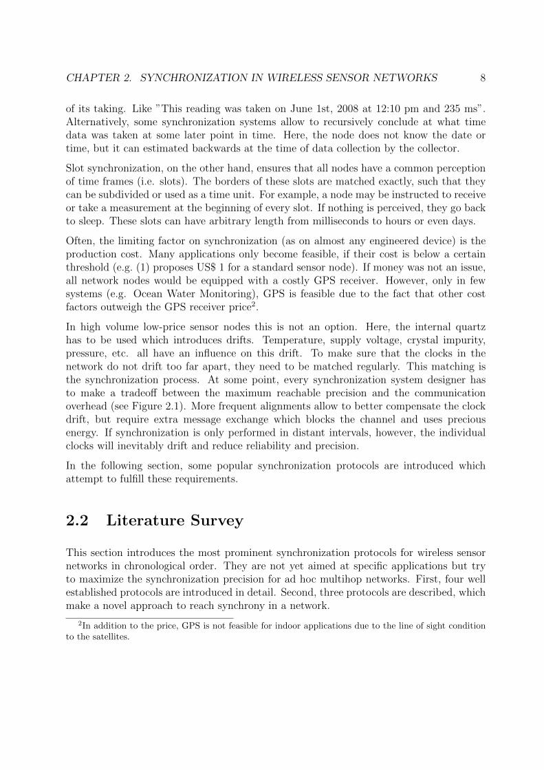
In high volume low-price sensor nodes this is not an option. Here, the internal quartzhas to be used which introduces drifts. Temperature, supply voltage, crystal impurity,pressure, etc. all have an influence on this drift. To make sure that the clocks in thenetwork do not drift too far apart, they need to be matched regularly. This matching isthe synchronization process. At some point, every synchronization system designer hasto make a tradeoff between the maximum reachable precision and the communicationoverhead (see Figure 2.1). More frequent alignments allow to better compensate the clockdrift, but require extra message exchange which blocks the channel and uses preciousenergy. If synchronization is only performed in distant intervals, however, the individualclocks will inevitably drift and reduce reliability and precision.
In the following section, some popular synchronization protocols are introduced whichattempt to fulfill these requirements.
2.2 Literature Survey
This section introduces the most prominent synchronization protocols for wireless sensornetworks in chronological order. They are not yet aimed at specific applications but tryto maximize the synchronization precision for ad hoc multihop networks. First, four wellestablished protocols are introduced in detail. Second, three protocols are described, whichmake a novel approach to reach synchrony in a network.
2In addition to the price, GPS is not feasible for indoor applications due to the line of sight conditionto the satellites.
CHAPTER 2. SYNCHRONIZATION IN WIRELESS SENSOR NETWORKS 9
Overhead
Price
Clock Accuracy
Compensation
Figure 2.1: The production price determines the possible inherent clock precision. A lessprecise clock requires more frequent compensation. Compensation creates communicationoverhead which is costly in regard to bandwidth and energy.
2.2.1 Prominent Synchronization Protocols
Wireline synchronization protocols like the Network Time Protocol (NTP) (9; 10) are notapplicable to WSNs due to their large memory requirements and comparably low precision(10 - 100ms). Therefore, in recent years several protocols have been proposed to createsynchrony between self-organizing network nodes, each of them tackling specific problemsarising in ad hoc networks, reaching precisions of up to 2.24 µs per hop (11; 12). However,high precision comes with a trade-off in complexity and scalability. Whilst designed forand tested in numbers of up to 60 nodes (12), it is yet open how these approaches willperform in numbers of several hundreds or thousands. Most of these established protocolshave been around for several years and have been tested and described in detail. Theseare the most prominent ones3:
Synchronization by Romer
Kay Romer’s approach from 200 (17) tried to address different challenges than many ofthe later to come synchronization protocols. Not aiming at a high precision, Romer devel-oped a technique to compare temporal relationships and realtime issues in sparse ad hocnetworks. The focus was for nodes to be able to communicate their measurements withtimestamps a posteriori, even if at the time of the real world occurence the nodes were notin communication proximity, for example in an inherently mobile sensor environment or a
3Several additional synchronization protocols have been suggested (13; 14; 15; 16) which explore dif-ferent aspects of synchronization in wireless networks, but are not directly connected to this work.
CHAPTER 2. SYNCHRONIZATION IN WIRELESS SENSOR NETWORKS 10
drive-by data collection setup. The protocol is not intended to synchronize all nodes of thenetwork to a common time. Instead, it only adjusts the timestamp of a message locally asit is passed to its destination. This is achieved through a round trip delay measurementon each hop. The achieved maximum precision of 3 ms (over 5 hops) is only sufficient forfew applications. Nevertheless, Romer’s work was one of the early practical approachesand was interpreted and improved by many synchronization protocols to follow.
Reference Broadcast Sychronization (RBS)
In 2002, Elson and Estrin (11) proposed the widely regarded Reference Broadcast Synchro-nization (RBS) which was tailored for sensor network requirements and adressed systemspecific delays in order to maximize precision, reaching 3 µs. The two major innovationswere the use of reference messages and the elimination of the non-deterministic hardwaredelays Send Time (propagation of a message through the OSI layers) and Access Time(time to wait until the channel is free). In RBS, any node can send a reference beaconsignal. All adjacent nodes who pick up this beacon timestamp it and then compare theirfindings with each other in order to adjust their internal clocks. Over time, all nodes willhave referenced and compared their findings and the network will synchronize. The mainstrength of RBS is its applicability to commodity hardware and existing software in sensornetworks.
Timing-sync Protocol for Sensor Networks (TPSN)
The Timing-sync Protocol for Sensor Networks (TPSN) (18), 2003, was a direct replyto RBS. Ganeriwal et al. specifically chose a strongly hierarchical approach, combinedwith pair-wise synchronization, while using some of RBS’ suggestions like reduction ofthe critical hardware delays. At first setup, a tree structure is established amongst equalnodes which from then on is the basis for top-down pair-wise synchronization. Duringeach synchronization hop the round trip time is measured. The constant updates fromthe surrounding nodes are used for correction of the internal clock. While TPSN arguesto be theoretically superior to RBS by a factor of 2 in terms of accuracy, the providedlaboratory test results are in the range of 17 µs which is below the 3 µs accuracy of RBS.The carefully established tree structure setup has not been tested towards robustness ormobility and appears to be a rather complex approach to synchronization. The authorsdid not go into detail how the protocol could support a sensor sleep mode without breakingthe tree structure. It is therefore to be seen how well TPSN synchronization will converge,perform and deliver in real world applications. However, it is noteworthy that TPSN wassimulated in an environment of 300 nodes. This is the largest test provided in a WSNsynchronization publication.
CHAPTER 2. SYNCHRONIZATION IN WIRELESS SENSOR NETWORKS 11
Flooding Time Synchronization Protocol (FTSP)
Maroti et al. (12) proposed the Flooding Time Synchronization Protocol (FTSP) in 2004,utilizing previous progress from RBS and TSPN. FTSP combines a dynamic flat nodehierarchy with medium access control (MAC) layer timestamping and clock correction.First, the node with the lowest ID is elected as master. The master node regularly floodsthe network with timing information. Eliminating most possible hardware delays the nodescommunicate single timestamps (no round trip information) through the network. Theinternal clocks are continually updated and corrected via linear regression. Remarkably,the authors ran a very large live experiment on 60 network nodes, testing on maliciousdevices, mobility and root election. Here, the average clock offset was 2.24 µs (maximum8, 64 µs), capping RBS. Also, this is the only approach for which the convergence time4 (15min equalling 30 synchronization rounds) is listed which can be a determining criterion forthe choice of a sychronization protocol.
2.2.2 Novel Synchronization Protocols
Whilst the previously described protocols use well-known procedures from computer net-working, all of the following go beyond the more traditional attempts in synchronizationand try to exploit the cooperative nature of wireless networks in more detail. Here, theadvantage is that theoretically the synchronization precision does not degrade over thenumber of hops, as it is reached through a consensus amongst nodes. As can be seenin a closer study, it is difficult to compare these suggestions with the above, since theyare strongly theoretical and (in their original descriptions) require different hardware thanstandard motes (apart from Tyrrell et al. (19)).
This novel suggestion comes from biology and is described in detail in Chapter 3.1. Inspiredby the phenomenon of thousands of fireflies gathering on trees in Malaysia and pulsingin synchrony, the approaches assume a very high number and density of nodes. Theseprotocols have only been simulated and not yet been technically implemented.
Scalable Synchronization Protocol
Inspired by the challenge of scalability and nature’s example for a solution in the formof Malaysian Fireflies, Scaglione et al. (20) propose a protocol for slot synchronizationwith minimal message overhead in 2005. Employing the PCO model (21) all nodes slowlyadjust to a pulse. The authors prove in theory that the nodes will quickly yield a commontime scale. Although making some assumptions regarding actual hardware and delays, thismodel is still very theoretical and makes no specification regarding precision. Simulationssuggest that the convergence time is optimally short. Scaglione et al. suggest to apply
4Convergence Time: Time to reach synchrony after startup
CHAPTER 2. SYNCHRONIZATION IN WIRELESS SENSOR NETWORKS 12
this system for a waveform ”reach-back”, where data can be transmitted over a longerdistance by the sensor group than each individual would have accomplished, for examplethrough pulse-position modulation. A strong practical drawback stems from the fact thatthis approach requires specific hardware that emits and senses the synchronization pulsesolely on the physical layer (i.e. no software interpretation).
Algorithmically Optimal Time Synchronization
Servetto et al. (22) propose a protocol that is very closely related to Scaglione et al. (20) andshares most of the ideas and conclusions. The two authors do not refer to each other andhave published in close succession. Picking up the problem of scalability in sensor networks,Servetto et al. suggest an approach where an elected and centrally located node initiatesregular pulses and data packets that propagate through the network. The surroundingnodes listen to the pulses and messages and ”tune in”. In this way, a synchonizationwaveform is established throughout the network. The election procedure for the masternode is not provided. Like Scaglione et al., Servetto et al. suggest to apply this methodto reach back to a distant receiver which can either be synchronized or obtain sensordata. Although the protocol proposes some innovations like node density dependent powerscaling, it is nearly identical to the Scalable Synchronization Protocol.
Firefly Role Model Synchronization
The most recent and most practical approach of the ”Firefly Models” is by Tyrrell etal. (19; 23). Based on Scaglione et al.’s findings, it transforms the model to transmissionmessages of non-zero length (i.e. no pulses) and works with some assumptions on delaysthat can occur in hardware. Also, node deafness during transmission is considered whichposes a major difference between off-the-shelf hardware and the theoretical model. Thisapproach is the basis for this work and is described in detail in Chapter 3.
2.3 Summary
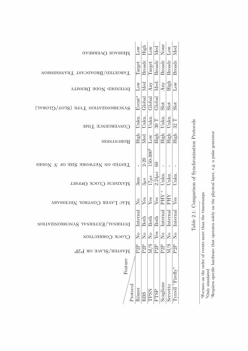
Table 2.1 summarizes all of the described protocols regarding key aspects.
Master/Slave or P2P Hierarchy is an important factor for the applicability of a proto-col. Do all nodes behave the same or does a master node exist? Whereas TPSN creates astrict tree hierarchy which make is sensible to topology changes, protocols like by Scaglioneet al. or Tyrrell et al. assume all network nodes to be equal members of a peer-to-peersystem.
CHAPTER 2. SYNCHRONIZATION IN WIRELESS SENSOR NETWORKS 13
Clock Correction For maximum accuracy it is indispensable to compensate for theinherent clock drift by internal clock correction in each network node. Although someprotocols do comment on this point, this survey states which ones have actively used clockcorrection to achieve higher precisions. Clock correction allows to space communicationintervals further apart, as each node ”learns” about its long term drifts.
Internal/External Synchronization Protocols strongly differ regarding their type oftime reference. Whereas RBS, TPSN and FTSP explicitly aim at distributing a (global)external reference time into the network, the other approaches only ensure that the clocksinside the network are synchronized, disregarding the external time frame.
MAC Layer Control Necessity For a wider usability on standard hardware, it isdesirable for a protocol to have little to no requirements regarding the medium accesscontrol or physical layer. For timestamping it is necessary to have limited access to thepacket queue in the radio chip, which several protocols require. The novel protocols,however, assume that extra radio hardware is available, aside from the standard radiocomponents.
Maximum Clock Offset This column reflects the maximum precision that each proto-col claims. Since some have only been simulated so far, no values are provided.
Tested Network Size Since scalability is a highly anticipated criterion in WSNs, it isdisplayed here, which network sizes (i.e. number of nodes) the authors have tested theirsystem on, if available.
Robustness Since node failures and topology changes can be expected in most scenarios,this column is an estimate of the protocol robustness by the author of this work. TPSNreceives a low rating due to the strict hierarchy of the approach. All P2P protocols can beexpected to possess high robustness due to their inherent self organization.
Convergence Time Although this is a very interesting parameter, it is only providedby two protocols. It describes the time a network requires to reach synchrony (startingfrom a random setting). Since comparison intervals differ, the duration is given in the unitof ”synchronization periods T”. For example, in FTSP T = 30 s.
Synchronization Type (Slot/Global) The protocols can be split into two groups(plus one special case) regarding the type of time they provide to the network. Either theyprovide a global reference (e.g. Universal Time Coordinated (UTC)) or create time slots
CHAPTER 2. SYNCHRONIZATION IN WIRELESS SENSOR NETWORKS 14
of predefined lengths. Romer’s suggestions focuses on the causal ordering of events morethan the exact time and is marked specifically.
Intended Node Density Synchronization protocols are specifically aimed at certaindensities. Sparse networks require a protocol to be robust and be able to reliably dis-tribute time over a single and unreliable link. High density network protocols use themultiple existing paths and broadcast nature to their advantage. When a protocol forsparse networks is deployed in a high density environment, contention may occur due totoo many messages occupying the channel. A high density protocol in a sparse networkmay not find the minimum number of nodes in range necessary to perform a synchroniza-tion step. Romer, for example, aims at nodes which may be out of reach for a long time.In contrast, Servetto et al. assumes that all nodes are in close proximity, if not even insingle hop range.
Targeted/Broadcast Transmission It is interesting for the classification of a protocolwhether it uses the broadcast property of the wireless channel or whether it behaves likein a wired system. For example, TPSN specifically addresses each node and only performsround trip measurements. Other protocols strongly base on the fact that a message willalways be heard by multiple receivers.
Message Overhead For energy efficiency, it is of prime importance how much radiocommunication is necessary to keep the network synchronized. This column is an estimateof the author, interpreting protocol descriptions. RBS receives a high overhead rating,because nodes always have to compare their perceived reference with all other nodes inrange, which may become a large number. Scaglione et al., in contrast, employs specialpulsing hardware which does not create message overhead.
XXX
XXX
XXX
XXX
Pro
toco
lF
eatu
re
Master/SlaveorP2P
ClockCorrection
Internal/ExternalSynchronization
MacLayerControlNecessary
MaximumClockOffset
TestedonNetworkSizeofNNodes
Robustness
ConvergenceTime
SynchronizationType(Slot/Global)
IntendedNodeDensity
Targeted/BroadcastTransmission
MessageOverhead
Rom
erP
2PN
oIn
tern
alN
o3m
s-
Hig
hU
nkn.
Eve
nta
Low
Tar
get
Low
RB
SP
2PN
oB
oth
Yes
3µs
2-20
Med
Unkn.
Glo
bal
Med
Bro
adc
Hig
hT
PSN
M/S
No
Bot
hY
es17µs
150-
300b
Low
Unkn.
Glo
bal
Any
Tar
get
Low
FT
SP
P2P
Yes
Bot
hY
es2.
24µs
60H
igh
30T
Glo
bal
Med
.B
road
cM
edSca
glio
ne
P2P
No
Inte
rnal
PH
Yc
Unkn.
-H
igh
Unkn.
Slo
tA
ny
Bro
adc
Non
eSer
vett
oM
/SN
oIn
tern
alP
HY
Unkn.
-H
igh
Unkn.
Slo
tH
igh
Bro
adc
Low
Tyrr
ell
”Fir
efly”
P2P
No
Inte
rnal
Yes
Unkn.
-H
igh
32T
Slo
tL
owB
road
cM
ed
Tab
le2.
1:C
ompar
ison
ofSynch
roniz
atio
nP
roto
cols
aF
ocu
ses
onth
eor
der
ofev
ents
mor
eth
anth
eti
mes
tam
ps
bO
nly
sim
ula
ted
cR
equ
ires
spec
ific
har
dw
are
that
oper
ates
sole
lyon
the
physi
cal
laye
r,e.
g.
ap
uls
egen
erato
r
Chapter 3
Firefly Synchronization
The present chapter introduces the biological phenomenon which inspired researchers toscrutinize a novel approach in synchronization. After following the research that has ledto the Firefly Protocol, the necessary adaptations are discussed which were made in thisthesis.
3.1 Biological Inspiration
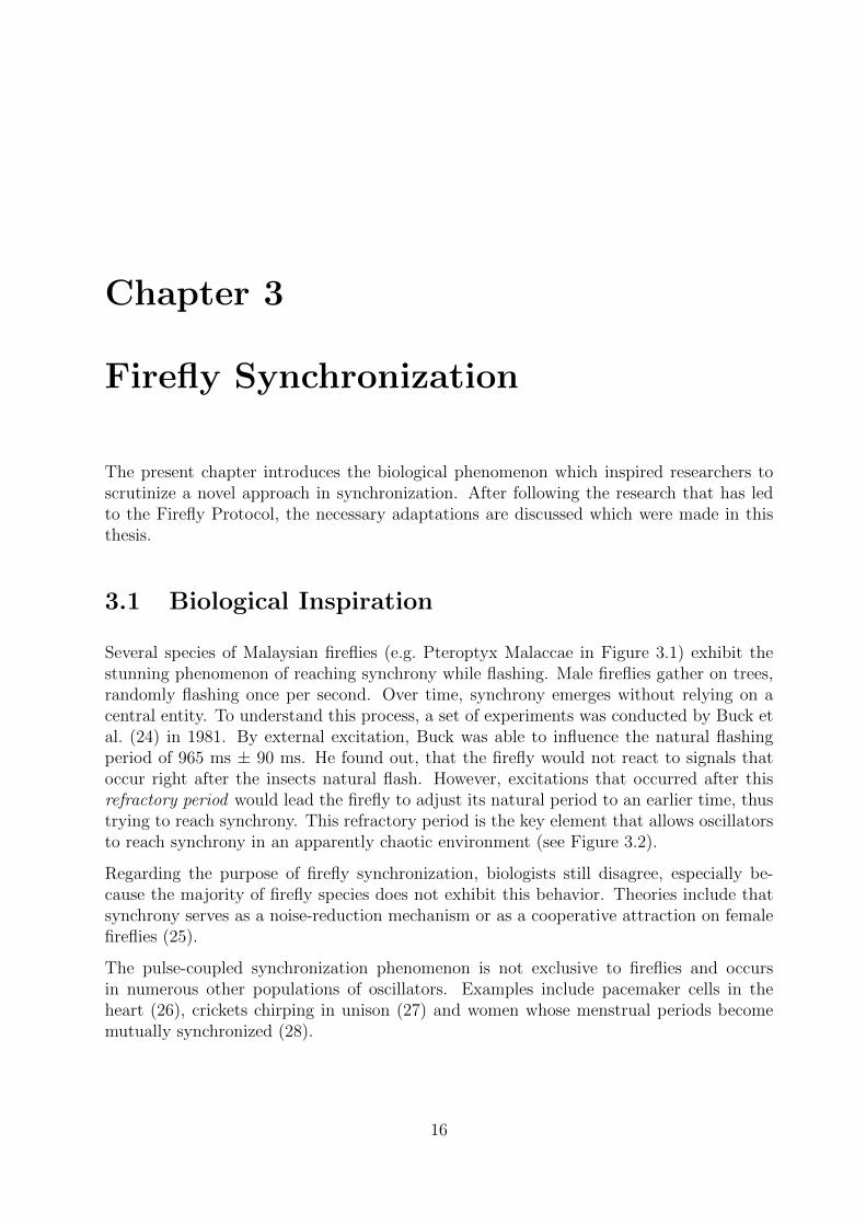
Several species of Malaysian fireflies (e.g. Pteroptyx Malaccae in Figure 3.1) exhibit thestunning phenomenon of reaching synchrony while flashing. Male fireflies gather on trees,randomly flashing once per second. Over time, synchrony emerges without relying on acentral entity. To understand this process, a set of experiments was conducted by Buck etal. (24) in 1981. By external excitation, Buck was able to influence the natural flashingperiod of 965 ms ± 90 ms. He found out, that the firefly would not react to signals thatoccur right after the insects natural flash. However, excitations that occurred after thisrefractory period would lead the firefly to adjust its natural period to an earlier time, thustrying to reach synchrony. This refractory period is the key element that allows oscillatorsto reach synchrony in an apparently chaotic environment (see Figure 3.2).
Regarding the purpose of firefly synchronization, biologists still disagree, especially be-cause the majority of firefly species does not exhibit this behavior. Theories include thatsynchrony serves as a noise-reduction mechanism or as a cooperative attraction on femalefireflies (25).
The pulse-coupled synchronization phenomenon is not exclusive to fireflies and occursin numerous other populations of oscillators. Examples include pacemaker cells in theheart (26), crickets chirping in unison (27) and women whose menstrual periods becomemutually synchronized (28).
16
CHAPTER 3. FIREFLY SYNCHRONIZATION 17
Figure 3.1: Pteroptyx Mallaccae (Source: www.rspg.org)
In 1990, Strogatz et al. (21) derived and proved a mathematical model for this phenomenon,called the Pulse-Coupled Oscillator (PCO), which is described in detail in the followingsection.
3.2 Pulse Coupled Oscillators (PCOs)
Inspired by a model for two interacting oscillators in cardiac pacemakers (29), Mirolloand Strogatz (21) extended the model to entire populations of oscillators (like fireflies), bysimplifying the dynamical phase function which describes the firing period. The internalclock of a firefly which determines the firing instant is modeled as an oscillator whichinteracts with other oscillators through discrete events (i.e. pulses).
Peskin describes the dynamics as
dxidt
= S0 − γxi, 0 ≤ xi ≤ 1, i = 1, ..., N.
When xi = 1, the ith oscillator ”fires” and xi jumps back to zero, for an initial conditionS0, dissipation γ and N oscillators.
Strogatz et al. lift the differential equation condition by assuming that x will increasemonotonically and smoothly from 0 to 1, described by a phase function φi(t). When φi(t)reaches 1, the oscillator ”fires” and φi(t) is reset to zero. If not coupled to other oscillators,it will naturally fire with period T .
When coupling occurs (i.e. two oscillators fire in each others’ range), the phase functionwill be adjusted as follows:
{φj(τj) = 0
φj(τj) = φi(τj) + ∆φ(φi(τj)) for i 6= j
CHAPTER 3. FIREFLY SYNCHRONIZATION 18
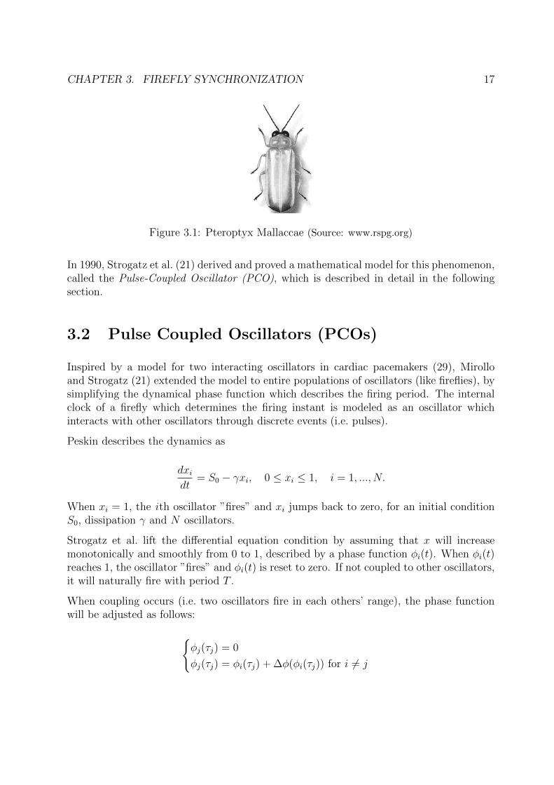
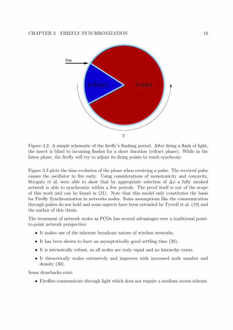
Figure 3.2: A simple schematic of the firefly’s flashing period. After firing a flash of light,the insect is blind to incoming flashes for a short duration (refract phase). While in thelisten phase, the firefly will try to adjust its firing points to reach synchrony.
Figure 3.3 plots the time evolution of the phase when receiving a pulse. The received pulsecauses the oscillator to fire early. Using considerations of monotonicity and concavity,Strogatz et al. were able to show that by appropriate selection of ∆φ a fully meshednetwork is able to synchronize within a few periods. The proof itself is out of the scopeof this work and can be found in (21). Note that this model only constitutes the basisfor Firefly Synchronization in networks nodes. Some assumptions like the communicationthrough pulses do not hold and some aspects have been extended by Tyrrell et al. (19) andthe author of this thesis.
The treatment of network nodes as PCOs has several advantages over a traditional point-to-point network perspective:
• It makes use of the inherent broadcast nature of wireless networks.
• It has been shown to have an asymptotically good settling time (20).
• It is intrinsically robust, as all nodes are truly equal and no hierarchy exists.
• It theoretically scales extensively and improves with increased node number anddensity (30).
Some drawbacks exist:
• Fireflies communicate through light which does not require a medium access scheme.

CHAPTER 3. FIREFLY SYNCHRONIZATION 19
Figure 3.3: Time evolution of the phase function in the Firefly Protocol (23)
Wireless networks, on the other hand, rely on carrier sense multiple access (CSMA).This imposes a strong limitation on precision and scalability.
• Compared to most other sensor synchronization protocols this approach synchronizesslots instead of a universal time reference. Some sensor applications may require auniversal time frame.
3.3 Application to Wireless Networks - The Firefly
Protocol
The PCO model (see Chapter 3.2) has inspired numerous research groups (19; 22; 31; 20)to look into possible applications in communication networks. The most interesting beingby Tyrrell et al. (23), because it tackles specific challenges common to wireless networksand is closest to an implementation on commodity hardware like MICAz.
Three issues are specifically addressed that allow utilization of the PCO model in networknodes:
• Node deafness during transmission
• Non-zero message length
• Processing delay
Node Deafness Network nodes are usually equipped with a single radio chipset thatcan either send or receive with a tuning interval in between the two states. Therefore, a
CHAPTER 3. FIREFLY SYNCHRONIZATION 20
node is ”deaf” while it transmits a message. If the PCO model were directly applied tonetwork nodes the attainable precision would be lower bound by the message transmissiontime TTX . While a node is transmitting, it is unable to recognize or interpret anothernode’s synchronization message. For example, at 250 kbits/sec an 18 byte message wouldtake 576 µs to transmit. This limit on precision is clearly unacceptable.
To overcome this limitation, Tyrrell et al. suggest to (randomly) create two groups in thenetwork, each transmitting and listening in turn. Therefore, group A would be transmittingwhile group B listens and group A can then adjust its timing when B transmits.
Non-Zero Message Length Pulses (as suggested by Scaglione et al. (32)) are not agood option in radio communication systems since they require special hardware and arevirtually impossible to detect. Rather, a synchronization word is used, which can berecognized by all receivers. Since a synchronization message has non-zero length, the PCOmodel has to be adapted. Tyrrell et al. suggest to reserve a fixed amount of time for thetransmission of radio signals.
Processing Delay Similar to the finite message length problem, the PCO model has tobe modified since digital receivers require significant encoding and decoding time. Marotiet al. (12) set these delays at around 200µs. To allow the system to still synchronize, thesedelays have to be accounted for.
3.4 Phase Diagram
Combining these three challenges results in the Firefly phase diagram (Figure 3.4), whichcreates two groups of transmitters and reserves a transmission window TTX .
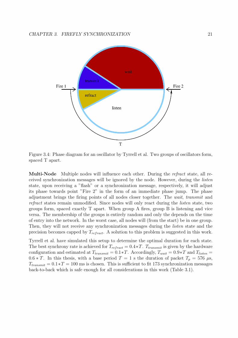
Single Node When a node with Firefly Synchronization is switched on it will oscillatewith period 2 T, starting at the point ”Fire 1”. It will run through the refract state,where the node ignores all synchronization influences. During the succeeding listen state,the node is susceptible to synchronization signals. If no messages are received, it willmove into the wait state, which is similar to refract. At the end of the wait state, thenode will internally issue the firing command. Because of the processing delay, this hasto occur exactly on time such that the message will leave the transmitter at point ”Fire1”. Therefore, according to Tyrrell et al., the transmit state is as long as the internalprocessing time of the node. After the message has left the transmitter at point ”Fire 1”,the cycle will reiterate.
CHAPTER 3. FIREFLY SYNCHRONIZATION 21
Figure 3.4: Phase diagram for an oscillator by Tyrrell et al. Two groups of oscillators form,spaced T apart.
Multi-Node Multiple nodes will influence each other. During the refract state, all re-ceived synchronization messages will be ignored by the node. However, during the listenstate, upon receiving a ”flash” or a synchronization message, respectively, it will adjustits phase towards point ”Fire 2” in the form of an immediate phase jump. The phaseadjustment brings the firing points of all nodes closer together. The wait, transmit andrefract states remain unmodified. Since nodes will only react during the listen state, twogroups form, spaced exactly T apart. When group A fires, group B is listening and viceversa. The membership of the groups is entirely random and only the depends on the timeof entry into the network. In the worst case, all nodes will (from the start) be in one group.Then, they will not receive any synchronization messages during the listen state and theprecision becomes capped by Trefract. A solution to this problem is suggested in this work.
Tyrrell et al. have simulated this setup to determine the optimal duration for each state.The best synchrony rate is achieved for Trefract = 0.4∗T . Ttransmit is given by the hardwareconfiguration and estimated at Ttransmit = 0.1∗T . Accordingly, Twait = 0.9∗T and Tlisten =0.6 ∗ T . In this thesis, with a base period T = 1 s the duration of packet Tp = 576 µs,Ttransmit = 0.1∗T = 100 ms is chosen. This is sufficient to fit 173 synchronization messagesback-to-back which is safe enough for all considerations in this work (Table 3.1).
CHAPTER 3. FIREFLY SYNCHRONIZATION 22
State wait transmit/TX refract listenDuration [ms] 900 100 400 600
Table 3.1: State durations used in this work
3.5 Modifications of the Firefly Model in this Work
Although the Firefly Protocol introduces some powerful ideas that bring the PCO modelcloser to actual hardware, there are several significant weaknesses which have to be coun-tered, before an implementation on network nodes is possible.
In order to implement Firefly Synchronization in a functional manner, some previous as-sumptions no longer hold and have to be adapted:
1. No constant transmission timing possible (12)
2. Medium access control
3. Immediate phase jump (22)
4. Dead lock case elimination
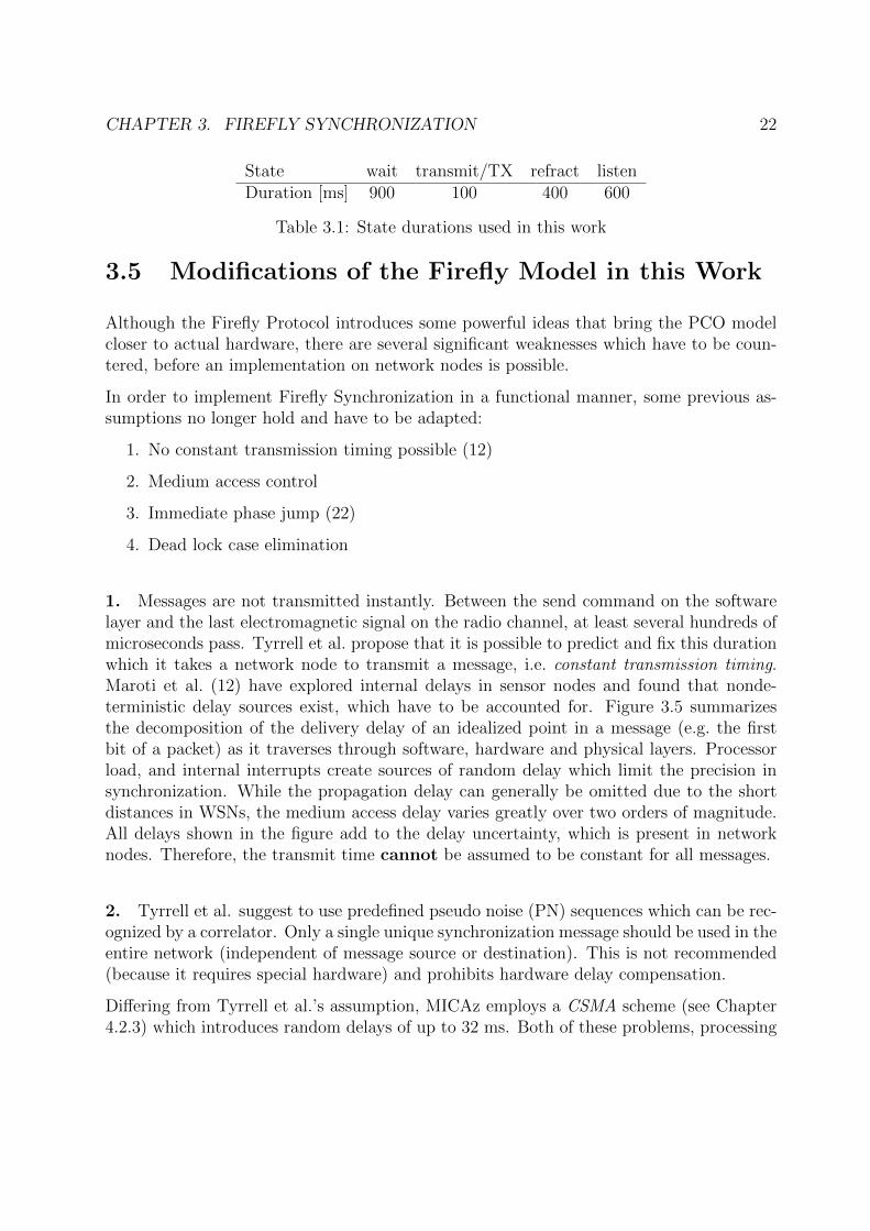
1. Messages are not transmitted instantly. Between the send command on the softwarelayer and the last electromagnetic signal on the radio channel, at least several hundreds ofmicroseconds pass. Tyrrell et al. propose that it is possible to predict and fix this durationwhich it takes a network node to transmit a message, i.e. constant transmission timing.Maroti et al. (12) have explored internal delays in sensor nodes and found that nonde-terministic delay sources exist, which have to be accounted for. Figure 3.5 summarizesthe decomposition of the delivery delay of an idealized point in a message (e.g. the firstbit of a packet) as it traverses through software, hardware and physical layers. Processorload, and internal interrupts create sources of random delay which limit the precision insynchronization. While the propagation delay can generally be omitted due to the shortdistances in WSNs, the medium access delay varies greatly over two orders of magnitude.All delays shown in the figure add to the delay uncertainty, which is present in networknodes. Therefore, the transmit time cannot be assumed to be constant for all messages.
2. Tyrrell et al. suggest to use predefined pseudo noise (PN) sequences which can be rec-ognized by a correlator. Only a single unique synchronization message should be used in theentire network (independent of message source or destination). This is not recommended(because it requires special hardware) and prohibits hardware delay compensation.
Differing from Tyrrell et al.’s assumption, MICAz employs a CSMA scheme (see Chapter4.2.3) which introduces random delays of up to 32 ms. Both of these problems, processing
CHAPTER 3. FIREFLY SYNCHRONIZATION 23
Figure 3.5: Delay estimates for an idealized point of a message (e.g. a data bit) throughthe components of two network nodes in a transmission system with estimated associateddelays
and MAC delay, can be solved by a technique employed in numerous synchronizationprotocols, called MAC layer time stamping (12; 11; 18), which works as follows:
When a transmit command is issued, the synchronization message is properly establishedand queued for transmission. However, when - on the physical layer - the transmission ofthe first bit starts, ”last minute” time stamping is performed. In a previously reserved placewithin the message a time value is inserted while the beginning of the message is alreadybeing transmitted. This is done in the memory of the radio chip. The time stampingallows to write additional information into the message, regarding how long the creationand processing of the message took the transmitter. In turn, this enables all receivers ofthis message to calculate when the send command was issued and eliminates the senderdelays, which would otherwise pose the bound on precision.
3. Two options exist how a node can react to a received synchronization message. Itcan either increase its internal phase slightly (suggested by (21)) and reach synchrony overseveral periods. Or it can immediately adjust its phase to ”fire”, i.e. perform a phase
CHAPTER 3. FIREFLY SYNCHRONIZATION 24
jump (22). In reference to the phase diagram, Figure 3.4, a stepwise increase would meanto shorten the listen phase slightly after the reception of a message. In case of a phasejump scheme, the listen state would be ended immediately, followed by the wait state. Inthis thesis, the immediate phase jump option is chosen to minimize convergence time.
4. Tyrrell et al.’s scheme divides the network in two groups. As mentioned earlier, adead lock case exists where all nodes may (by accident) be part of the same group. Theprobability of this occurrence is highest for scarce networks and depends on the durationof the refract state. A solution to this problem is proposed here. The protocol has beenadapted to keep a counter of periods which are missing incoming synchronization messages.If for a number of nP periods, no synchronization message has been received a node mayeither be out of radio range of other nodes or locked up in the same group, where nP is arandom number between 10 and 25. Therefore, it will repeat its listening state and resetthe counter. This assures that after no more than nP cycles the groups will be separatedagain.
3.6 Firefly 2.0
This section brings the above considerations together, and describes the details of thesynchronization protocol as implemented in this thesis. Succinctly, the implementation ofthe Firefly Protocol on MICAz network nodes required the protocol from Tyrrell et al.,the methods regarding delays and precision from Maroti et al. and the infrastructure andcontrol provided by TinyOS. It is called ”Firefly 2.0”. Only combining these three keyelements and the four adaptations from the previous section results in a functioning andprecisely running system.
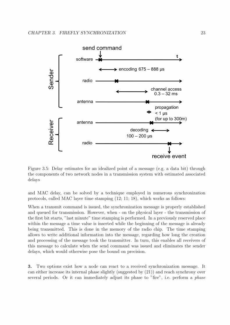
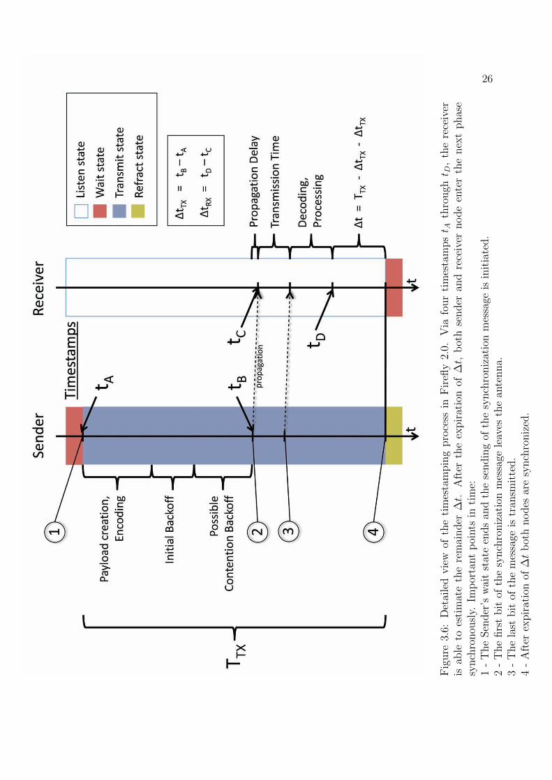
Figure 3.6 goes into detail regarding delay handling as it is performed in Firefly 2.0. TheFigure is a more precise view of the transmit state from Figure 3.4. Firstly, a fixed timeinterval is reserved for the transmission of all synchronization messages, TTX . This in-terval has to be chosen large enough to fit all synchronization messages in a high trafficenvironment and is determined by the contention of the network. Since a higher nodedensity creates more messages, TTX should be larger for higher densities or the contentionbackoff must be limited for all nodes. It must under all circumstances be prevented thatsynchronization messages are still being sent after expiration of the transmit phase.
Whenever a node finishes the wait state and enters the transmit state, it commands thetransmission of a synchronization message and marks the command time with a timestamptA. After processing (encoding delay) and the initial backoff, the channel will be checkedfor clearance. Depending on traffic, additional delays may occur through the contentionbackoff. When the message is then ready to be sent, up to 32 ms may have passed.Now, when the first byte of the message is being transmitted onto the radio channel, it is

CHAPTER 3. FIREFLY SYNCHRONIZATION 25
timestamped for a second time with timestamp tB. The difference of ∆tTX = tB − tA iswritten into the outgoing message.
In the receiver, a similar procedure is implemented. Upon the first received byte, a times-tamp tC is created. When the message is entirely received, aligned, decoded and found tobe a synchronization message, it is recorded again with timestamp tD. ∆tRX = tD − tCis the processing time of the receiver. Knowledge of ∆tTX and ∆tRX allows the receiverto infer when the sending command was given. Since the duration of the transmit phaseTTX is predefined, the receiver can count down the remainder of this duration and beginthe wait state at the same instant as the transmitter enters the refract state, thus reachingsynchrony.
CHAPTER 3. FIREFLY SYNCHRONIZATION 26
Fig
ure
3.6:
Det
aile
dvie
wof
the
tim
esta
mpin
gpro
cess
inF
irefl
y2.
0.V
iafo
ur
tim
esta
mpst A
thro
ugh
t D,
the
rece
iver
isab
leto
esti
mat
eth
ere
mai
nder
∆t.
Aft
erth
eex
pir
atio
nof
∆t,
bot
hse
nder
and
rece
iver
node
ente
rth
enex
tphas
esy
nch
ronou
sly.
Imp
orta
nt
poi
nts
inti
me:
1-
The
Sen
der
’sw
ait
stat
een
ds
and
the
sendin
gof
the
synch
roniz
atio
nm
essa
geis
init
iate
d.
2-
The
firs
tbit
ofth
esy
nch
roniz
atio
nm
essa
gele
aves
the
ante
nna.
3-
The
last
bit
ofth
em
essa
geis
tran
smit
ted.
4-
Aft
erex
pir
atio
nof
∆t
bot
hnodes
are
synch
roniz
ed.
Chapter 4
The MICAz Network Node
This chapter introduces the MICAz network node (Section 4.1) on which the synchroniza-tion protocol for the present work was implemented in detail. It provides all necessaryinformation to perform operations relevant to timing.
4.1 TinyOS Programming on MICAz
IEEE 802.15.4 / ZigBee
”IEEE Std 802.15.4-2003 defined the protocol and compatible interconnection for datacommunication devices using low-data-rate, low-power, and low-complexity short-rangeradio frequency (RF) transmissions in a wireless personal area network (WPAN).”1 TheIEEE standard specifies the network topologies, architecture, MAC aspects as well asphysical layer details necessary to design a compliant network node. All Berkeley motes(like MICAz) are designed according to this standard.
The IEEE standard is extended by the ZigBee specification2 which enables network exten-sions like discovery, multicasting or security. It is not directly involved in this synchroniza-tion protocol and is mentioned here only for a complete description of the MICAz networknode.
MICAz
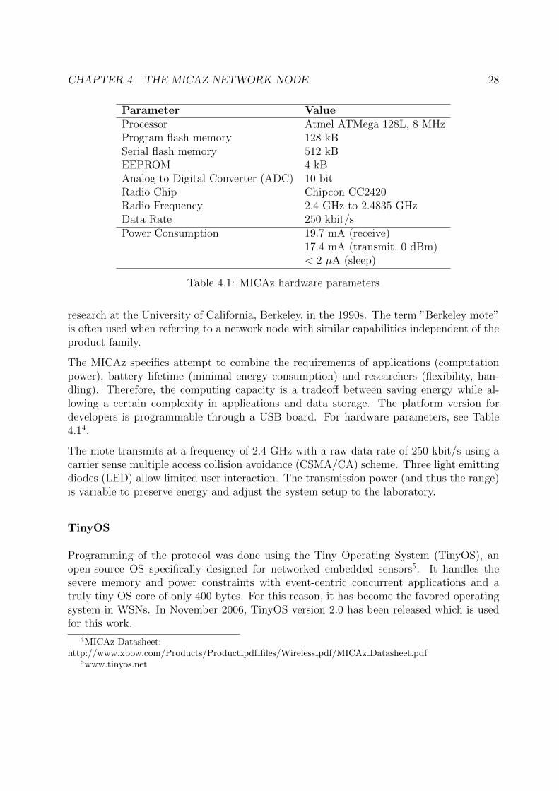
The MICAz (Figure 4.1) is the latest generation of MICA Motes from Crossbow Technol-ogy3. The term ”mote” refers to a node in a wireless sensor network and was coined during
1http://ieeexplore.ieee.org/servlet/opac?punumber=42994942www.zigbee.org3www.xbow.com
27
CHAPTER 4. THE MICAZ NETWORK NODE 28
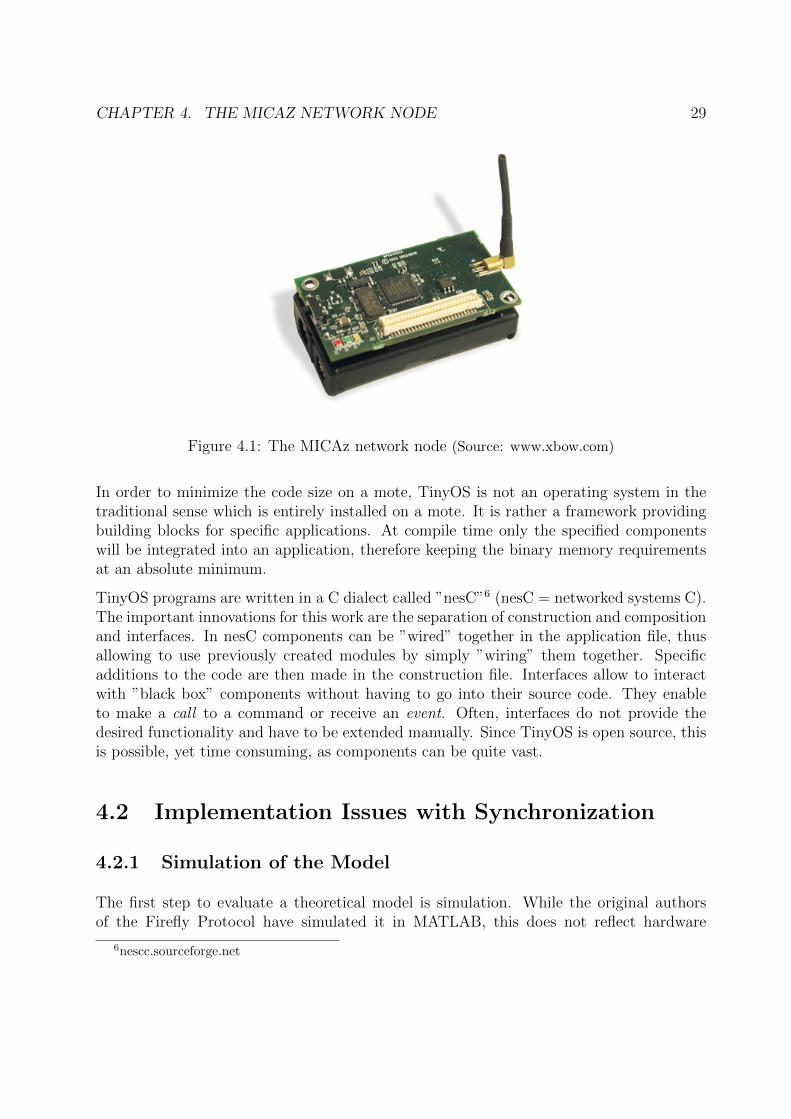
Parameter ValueProcessor Atmel ATMega 128L, 8 MHzProgram flash memory 128 kBSerial flash memory 512 kBEEPROM 4 kBAnalog to Digital Converter (ADC) 10 bitRadio Chip Chipcon CC2420Radio Frequency 2.4 GHz to 2.4835 GHzData Rate 250 kbit/sPower Consumption 19.7 mA (receive)
17.4 mA (transmit, 0 dBm)< 2 µA (sleep)
Table 4.1: MICAz hardware parameters
research at the University of California, Berkeley, in the 1990s. The term ”Berkeley mote”is often used when referring to a network node with similar capabilities independent of theproduct family.
The MICAz specifics attempt to combine the requirements of applications (computationpower), battery lifetime (minimal energy consumption) and researchers (flexibility, han-dling). Therefore, the computing capacity is a tradeoff between saving energy while al-lowing a certain complexity in applications and data storage. The platform version fordevelopers is programmable through a USB board. For hardware parameters, see Table4.14.
The mote transmits at a frequency of 2.4 GHz with a raw data rate of 250 kbit/s using acarrier sense multiple access collision avoidance (CSMA/CA) scheme. Three light emittingdiodes (LED) allow limited user interaction. The transmission power (and thus the range)is variable to preserve energy and adjust the system setup to the laboratory.
TinyOS
Programming of the protocol was done using the Tiny Operating System (TinyOS), anopen-source OS specifically designed for networked embedded sensors5. It handles thesevere memory and power constraints with event-centric concurrent applications and atruly tiny OS core of only 400 bytes. For this reason, it has become the favored operatingsystem in WSNs. In November 2006, TinyOS version 2.0 has been released which is usedfor this work.
4MICAz Datasheet:http://www.xbow.com/Products/Product pdf files/Wireless pdf/MICAz Datasheet.pdf
5www.tinyos.net
CHAPTER 4. THE MICAZ NETWORK NODE 29
Figure 4.1: The MICAz network node (Source: www.xbow.com)
In order to minimize the code size on a mote, TinyOS is not an operating system in thetraditional sense which is entirely installed on a mote. It is rather a framework providingbuilding blocks for specific applications. At compile time only the specified componentswill be integrated into an application, therefore keeping the binary memory requirementsat an absolute minimum.
TinyOS programs are written in a C dialect called ”nesC”6 (nesC = networked systems C).The important innovations for this work are the separation of construction and compositionand interfaces. In nesC components can be ”wired” together in the application file, thusallowing to use previously created modules by simply ”wiring” them together. Specificadditions to the code are then made in the construction file. Interfaces allow to interactwith ”black box” components without having to go into their source code. They enableto make a call to a command or receive an event. Often, interfaces do not provide thedesired functionality and have to be extended manually. Since TinyOS is open source, thisis possible, yet time consuming, as components can be quite vast.
4.2 Implementation Issues with Synchronization
4.2.1 Simulation of the Model
The first step to evaluate a theoretical model is simulation. While the original authorsof the Firefly Protocol have simulated it in MATLAB, this does not reflect hardware
6nescc.sourceforge.net
CHAPTER 4. THE MICAZ NETWORK NODE 30
effects like delays, which are the central issue of this thesis. Another option, here, isTOSSIM (33), a simulator provided along with TinyOS (TOSSIM = TinyOS SIMulator).It permits increased interaction capabilities which is especially useful for debugging, asit is particularly difficult to find the source of an error in a network node, if the onlyhuman interaction interfaces are three LEDs. However, TOSSIM does not implement timeconsumption and therefore assumes every function call to finish instantly. Also, physicalnetwork aspects like medium access control are only marginally fitted. For these reasonsit was not used in this work and is only mentioned for completeness.
4.2.2 Time and Clocking on MICAz
Regarding timing, no interfaces or components are provided by TinyOS that go beyond theabsolute basics. There is no internal representation for time stamps like minutes, hoursor days. Probably, because of the numerous platforms which TinyOS supports and therequirements towards precision that are not yet defined, this functionality is still to besupplied.
All clocking and timing functions on a MICAz radio mote are provided by the onboard mi-crocontroller, ATmega128L7. The microcontroller is clocked at f0 = 7.3728 MHz. All timedoperations base on f0, but different derivations exist. The flexible millisecond timer (namedTimerMilliC in TinyOS) increments every 32 ticks of a Jiffy = 32,768 Hz = 30.518 µs, i.e.1024 times per second. The more precise microsecond counter (CounterMicro32C) runsat f1 = f0/8 = 0.9216 Mhz (Table 4.2). This counter is linked to the chip over compareregisters. Therefore, the number of simultaneous counters is limited to three, whereas avirtually unlimited number of timers can be created. After initially using both timers inthis project, the program was later slimmed to run all operations on a single microsecondcounter.
Name MilliC 32kHz MicroCFrequency 1,024 Hz 32,768 Hz 0.9216 MHzPeriod 976 ms 30.518 µs 1.084 µs
Table 4.2: Available timer precisions in TinyOS/MICAz
This leads to the fact that all clock values used in this thesis are of unit clock ticks, whichis
1 clocktick = 1/f1 = 1/0.9216 MHz = 1.085µs.
The timer and counter components are precise up to the accuracy of the system clock. Theinitial starting of a timer costs between 100 and 500 µs. However, every successive startor stop of that timer is correct to the microsecond.
7http://www.atmel.com/dyn/resources/prod documents/doc2467.pdf
CHAPTER 4. THE MICAZ NETWORK NODE 31
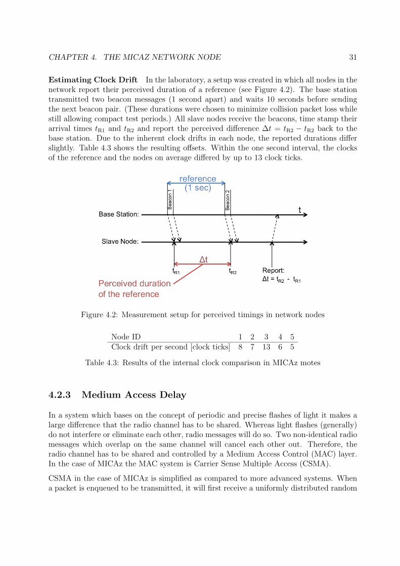
Estimating Clock Drift In the laboratory, a setup was created in which all nodes in thenetwork report their perceived duration of a reference (see Figure 4.2). The base stationtransmitted two beacon messages (1 second apart) and waits 10 seconds before sendingthe next beacon pair. (These durations were chosen to minimize collision packet loss whilestill allowing compact test periods.) All slave nodes receive the beacons, time stamp theirarrival times tR1 and tR2 and report the perceived difference ∆t = tR2 − tR2 back to thebase station. Due to the inherent clock drifts in each node, the reported durations differslightly. Table 4.3 shows the resulting offsets. Within the one second interval, the clocksof the reference and the nodes on average differed by up to 13 clock ticks.
Figure 4.2: Measurement setup for perceived timings in network nodes
Node ID 1 2 3 4 5Clock drift per second [clock ticks] 8 7 13 6 5
Table 4.3: Results of the internal clock comparison in MICAz motes
4.2.3 Medium Access Delay
In a system which bases on the concept of periodic and precise flashes of light it makes alarge difference that the radio channel has to be shared. Whereas light flashes (generally)do not interfere or eliminate each other, radio messages will do so. Two non-identical radiomessages which overlap on the same channel will cancel each other out. Therefore, theradio channel has to be shared and controlled by a Medium Access Control (MAC) layer.In the case of MICAz the MAC system is Carrier Sense Multiple Access (CSMA).
CSMA in the case of MICAz is simplified as compared to more advanced systems. Whena packet is enqueued to be transmitted, it will first receive a uniformly distributed random
CHAPTER 4. THE MICAZ NETWORK NODE 32
time offset (Initial Backoff) with limits defined in the IEEE 802.15.4 standard. Afterthis initial delay, the transmitter checks the channel for transmissions. In case the ClearChannel Assessment (CCA) returns a busy channel, the packet will once again be put onhold for a random amount of time (Congestion Backoff). This procedure is repeated untilthe channel is found to be clear and the packet can be transmitted. The risk of two motesboth simultaneously recognizing the channel as free and transmitting - thus eliminatingeach other - still exists. Also, other MAC specific problems like the Hidden Terminal ormessage acknowledgment are not addressed in the standard and are left to the applicationlayer (34; 35).
In MICAz motes, unexpectedly, the CSMA protocol is software controlled. This means thatthe radio chip takes orders from the CPU and reports back with flags and will not makedecisions on its own. The advantage is here, that the programmer can take direct influenceon the CCA and backoff intervals over the RadioBackoff interface. For each individualmessage, CCA can be allowed or disallowed and the backoffs separately configured. Thisinformation is contained within the TinyOS system libraries for the CC2420 chipset.
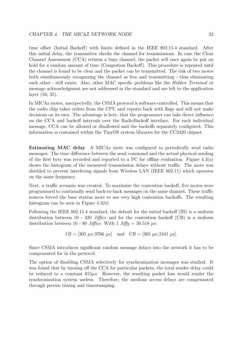
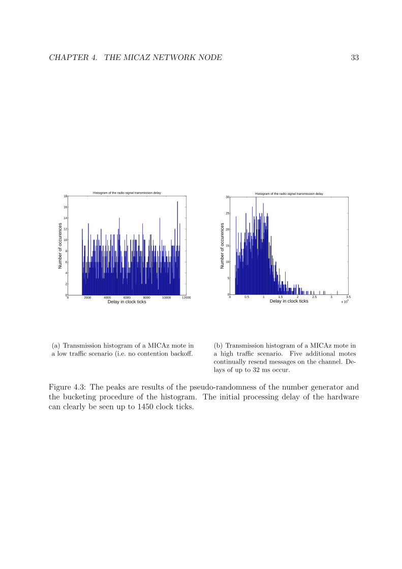
Estimating MAC delay A MICAz mote was configured to periodically send radiomessages. The time difference between the send command and the actual physical sendingof the first byte was recorded and reported to a PC for offline evaluation. Figure 4.3(a)shows the histogram of the measured transmission delays without traffic. The mote wasshielded to prevent interfering signals from Wireless LAN (IEEE 802.11) which operateson the same frequency.
Next, a traffic scenario was created. To maximize the contention backoff, five motes wereprogrammed to continually send back-to-back messages on the same channel. These trafficsources forced the base station mote to use very high contention backoffs. The resultinghistogram can be seen in Figure 4.3(b)
Following the IEEE 802.15.4 standard, the default for the initial backoff (IB) is a uniformdistribution between 10 - 320 Jiffies and for the contention backoff (CB) is a uniformdistribution between 10 - 80 Jiffies. With 1 Jiffy = 30.518 µs:
IB = [305 µs; 9766 µs] and CB = [305 µs; 2441 µs].
Since CSMA introduces significant random message delays into the network it has to becompensated for in the protocol.
The option of disabling CSMA selectively for synchronization messages was studied. Itwas found that by turning off the CCA for particular packets, the total sender delay couldbe reduced to a constant 655µs. However, the resulting packet loss would render thesynchronization system useless. Therefore, the medium access delays are compensatedthrough precise timing and timestamping.
CHAPTER 4. THE MICAZ NETWORK NODE 33
0 2000 4000 6000 8000 10000 120000
2
4
6
8
10
12
14
16
18Histogram of the radio signal transmission delay
Delay in clock ticks
Num
ber
of o
ccur
ence
s
(a) Transmission histogram of a MICAz mote ina low traffic scenario (i.e. no contention backoff.
0 0.5 1 1.5 2 2.5 3 3.5
x 104
0
5
10
15
20
25
30Histogram of the radio signal transmission delay
Delay in clock ticks
Num
ber
of o
ccur
ence
s
(b) Transmission histogram of a MICAz mote ina high traffic scenario. Five additional motescontinually resend messages on the channel. De-lays of up to 32 ms occur.
Figure 4.3: The peaks are results of the pseudo-randomness of the number generator andthe bucketing procedure of the histogram. The initial processing delay of the hardwarecan clearly be seen up to 1450 clock ticks.
Chapter 5
Implementation
Up to this point, the necessary background for the implementation has been provided.This chapter covers what implementation details were necessary to realize Firefly Synchro-nization on MICAz motes, and summarizes the central issues from chapter 4.
5.1 Important Issues
Communication Firstly, the behavior of MICAz motes regarding communication is notdistinct, since the IEEE standard 802.15.4 leaves many options open which can be config-ured on the software level. It was found that acknowledgment of messages is not inherentlyactive and the nodes follow a ”fire and forget” scheme. Therefore, packet loss can not bedetected by a node. For synchronization, this is advantageous since a possible re-requestof messages introduces large delays which need to be avoided if possible. Also, there is nolimit on the number of contention backoffs taken when the channel is found to be busy.Theoretically, if the channel were continuously busy, a node would never send a packet andat the same time never drop the packet.
When running unmodified, frequent packet losses occur because of the simple CSMAscheme applied. Therefore, to increase packet delivery reliability it is useful to add anadditional random component to transmit times even before the CSMA process is initi-ated. In addition to the radio channel packet loss, the serial port poses a bottleneck. Ithas a lower bit-rate than the radio channel and in the case of burst traffic (at the synchro-nization points) frequent packet losses occur. This problem was solved by adding a packetqueue to the base station mote.
TinyOS version 2.x Secondly, major changes were made to the system core of TinyOSduring the transition from version 1.x to 2.x. Source code for version 1.x will not compileunder 2.x. This means that any applications developed before the release of 2.x have to be
34
CHAPTER 5. IMPLEMENTATION 35
converted and to date only few applications exist for 2.x. Many issues once solved have tobe resolved in new data structures. For example, access to the MAC layer time stampingwas changed significantly.
Time representation When implementing the protocol on the wireless nodes, it wasunclear how the representation of time works inside of a MICAz mote. No specific inter-face exists which allows for seamless access, conversion and modification of time. Threeprecisions of counting exist, milliseconds, 32 kHz (i.e. 32,768 clock ticks per second), andmicroseconds. These options were explored and the decision was clearly made for microsec-ond precision which offers the best resolution. For this accuracy, the counter component(which counts up and can be read out) and the alarm component (which counts down andfires on reaching zero) can be used.
Next, several components were explored which had to be discarded because of limitations.For example, the TinyOS provides a RadioTimeStamping interface, which allows to times-tamp incoming and outgoing radio messages. However, this timestamp is of size 8 bit =65,536 values. When running at 32 kHz, this creates an overflow every 2 seconds. Sincesynchronization intervals are much longer than this, this interface is not useful and thetimestamping was implemented manually.
Disabling the medium access control As described in Section 4.2.3 it is importantto estimate medium access which creates the dominating delays. An attempt was madeto follow Tyrrell et al.’s suggestions (19) of fixed transmit times by disabling the clearchannel assessment (CCA) of the CSMA scheme. This is possible, as the entire scheme isimplemented on software level. However, packet losses due to collisions by far outweighedpossible gains of the CCA shut-off. Therefore, timestamping was used instead.
MAC layer timestamping The previously mentioned and critically important MAClayer timestamping is possible via direct access to the radio chip (CC2420). The chipdesigners offer an interface, the CC2420Transmit, which allows to access the send bufferfrom software. If the internal bit offset is known, pieces of the send buffer memory canbe replaced. In this particular case it works as follows: An IEEE 802.15.4 radio messageconsists of a header and a data field. The header contains 11 bytes of meta information like,for example, message length, message source or message type. The data field is of variablelength. Knowledge of the header size and the position of the desired data piece inside themessage allow to modify a particular group of bytes in the memory. Extreme care has to betaken regarding this offset and the endianness of the layers in between. TinyOS providesthe network data type which internally corrects the endianness as necessary.
Practically, the operation runs as follows: On the software level a send command is issued.The data payload is constructed, filled and added to the header. The message is passedto the radio chip. The radio chip initiates the channel assessment of the CSMA scheme.
CHAPTER 5. IMPLEMENTATION 36
When the channel is found to be clear, the software layer is informed and calls the memorymodification function. This modification is, therefore, performed in the last moment whenthe header of the message is already being transmitted.
Files The protocol was programmed as a compact nesC component consisting of a headerfile, a configuration file and an implementation file1. The transition through the phasestates was realized through an alarm with microsecond precision that was instructed tostart, stop and reset as needed upon state changes. All nodes are programmed identically.
5.2 Measurement Setup
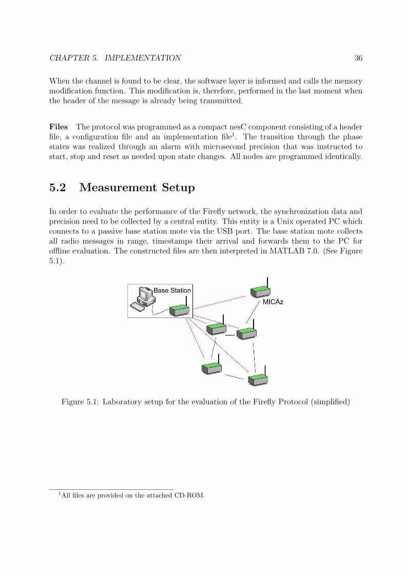
In order to evaluate the performance of the Firefly network, the synchronization data andprecision need to be collected by a central entity. This entity is a Unix operated PC whichconnects to a passive base station mote via the USB port. The base station mote collectsall radio messages in range, timestamps their arrival and forwards them to the PC foroffline evaluation. The constructed files are then interpreted in MATLAB 7.0. (See Figure5.1).
Figure 5.1: Laboratory setup for the evaluation of the Firefly Protocol (simplified)
1All files are provided on the attached CD-ROM.
Chapter 6
Results
Because of the inherent robustness and flexibility within the Firefly network, it is extremelydifficult to evaluate. Since there exists no external or network wide reference, what pointin time should be used for comparison? And since nodes are free to make mistakes orswitch groups, there is no immediate right or wrong for a mote, as long as the networkas a whole is clocked correctly. Since this approach creates a dynamical system, it is alsovery difficult to explain and predict its behavior. Small offsets or delays of a single nodemay disturb the entire system for several cycles.
To categorize and evaluate systems with a different number of nodes, the following criteriaand plots will be discussed:
1. Mean and variance of the offsets from the reference
2. Probability Distribution Function (PDF) of the offsets on a millisecond andmicrosecond scale, compared with the offset positions in each node
3. Cycle durations over time
4. Offsets from the reference plotted over time (to recognize specific network behavior)
Before going into detailed scenarios, the term ”reference” has to be clarified as it is notgiven by the system and has to be defined.
Regarding the Reference The point of reference in this evaluation is the average ofthe ”firing points”, in between 600 ms intervals. This means that if the base station (asdata collector) does not receive any messages for at least 600 ms, it considers it the startof a new interval. Within this interval, all message timestamps are averaged. This averageis treated as the reference from which the time offsets are calculated. For example, forthree nodes firing at ti = {2.9, 3.0, 3.1} the reference becomes tref = 3 and the offsetsare oi = {−0.1, 0, 0.1}. Since in this evaluation the average offset is equal to zero due to
37
CHAPTER 6. RESULTS 38
symmetry, all offset statistics are created from absolute values. In the example, the averageoffset is ‖oi‖ = 0.1.
Since the base station is a passive reader of the synchronization messages, it must be inrange of all network nodes. Thus, all systems analyzed are single hop networks with allnodes in range to each other. Such networks are also called fully meshed networks inliterature.
Cycle durations are calculated as the differences between the reference points in each group.Thus, a ”cycle” is a complete tour around the phase state circle (Figure 3.4) - not the halfcircle between two adjacent firings of Group A and Group B. A change in cycle durationscan shed light on a constant drift of the network due to, for example, asymmetries in thesynchronization period.
As stated in Section 4.2.2, clock ticks are the basis for all timing operations in a node andhave a duration of 1.085 µs. All measurements and operations base on this unit. However,for the sake of simplicity and without loss of generality, clock ticks will in this section betreated as having a duration of 1 µs. This makes plots and scales easier to understand.Since all nodes and instruments in the system count similarly, all results scale correctly toeach other and differ from reality through the factor 1.085.
The analysis is performed stepwise - with a higher number of nodes in each experiment -to go into specific aspects in turn as they appear in the more complicated systems.
6.1 Single Node Evaluation
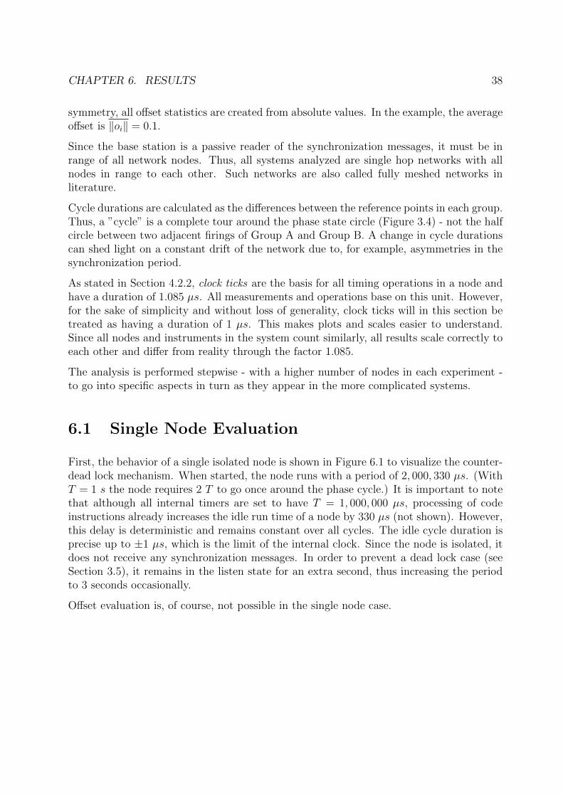
First, the behavior of a single isolated node is shown in Figure 6.1 to visualize the counter-dead lock mechanism. When started, the node runs with a period of 2, 000, 330 µs. (WithT = 1 s the node requires 2 T to go once around the phase cycle.) It is important to notethat although all internal timers are set to have T = 1, 000, 000 µs, processing of codeinstructions already increases the idle run time of a node by 330 µs (not shown). However,this delay is deterministic and remains constant over all cycles. The idle cycle duration isprecise up to ±1 µs, which is the limit of the internal clock. Since the node is isolated, itdoes not receive any synchronization messages. In order to prevent a dead lock case (seeSection 3.5), it remains in the listen state for an extra second, thus increasing the periodto 3 seconds occasionally.
Offset evaluation is, of course, not possible in the single node case.
CHAPTER 6. RESULTS 39
Figure 6.1: Cycle duration for a single isolated node. In most cases, the node ran witha period of approximately 2 seconds. It can be clearly seen that occasionally the noderepeats half of a period, amounting to 3 seconds. This is caused by the node trying tobreak a deadlock case as described in Section 3.5
6.2 Dual Node Evaluation
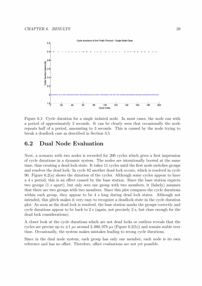
Next, a scenario with two nodes is recorded for 200 cycles which gives a first impressionof cycle durations in a dynamic system. The nodes are intentionally booted at the sametime, thus creating a dead lock state. It takes 11 cycles until the first node switches groupsand resolves the dead lock. In cycle 82 another dead lock occurs, which is resolved in cycle90. Figure 6.2(a) shows the duration of the cycles. Although some cycles appear to havea 4 s period, this is an effect caused by the base station. Since the base station expectstwo groups (1 s apart), but only sees one group with two members, it (falsely) assumesthat there are two groups with two members. Since this plot compares the cycle durationswithin each group, they appear to be 4 s long during dead lock states. Although notintended, this glitch makes it very easy to recognize a deadlock state in the cycle durationplot. As soon as the dead lock is resolved, the base station marks the groups correctly andcycle durations appear to be back to 2 s (again, not precisely 2 s, but close enough for thedead lock considerations).
A closer look at the cycle durations which are not dead locks or outliers reveals that thecycles are precise up to ±1 µs around 2, 000, 078 µs (Figure 6.2(b)) and remain stable overtime. Occasionally, the system makes mistakes leading to wrong cycle durations.
Since in the dual node system, each group has only one member, each node is its ownreference and has no offset. Therefore, offset evaluations are not yet possible.
CHAPTER 6. RESULTS 40
(a) The cycle durations illustrate how the systems behaves over time. The cycle duration duringthe dead lock is not actually twice as long, but is specifically marked by the base station to allowfor an easier display.
(b) On the small scale, cycle durations are precise within ±1 µs. The cycle durations are 78 µslonger than the designated 2 s due to small software processing delays (similar to the idle cycleduration).
Figure 6.2: Evaluation of the two node Firefly system
CHAPTER 6. RESULTS 41
6.3 Four Node System Evaluation
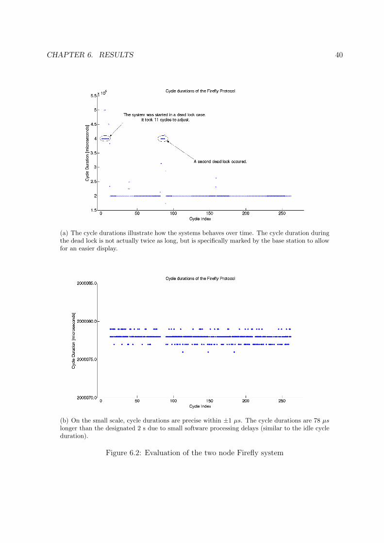
The four node system is analyzed, because it reaches maximum precision. The system islarge enough to have a group size > 1 , yet small enough to have a low probability ofrandom outliers. Figure 6.3 shows that on the millisecond scale, outliers still go as far as600 ms. However, 99 % of the values lie within 100 µs of each other, and 95 % are within5 µs. Disregarding outliers with an offset of more than 5 ms, this results in average offsetsbetween 1.5 µs and 4.5 µs (see Table 6.1).
Figure 6.3: Offset values and distribution of the four node Firefly system
Regarding cycle durations, details can be taken from Figure 6.4. Since the cycle durationsare calculated as the difference of two reference points, they are not constant and varywithin 20 - 30 µs of the mean at 2, 000, 084 µs. There are two dominating cycle durations
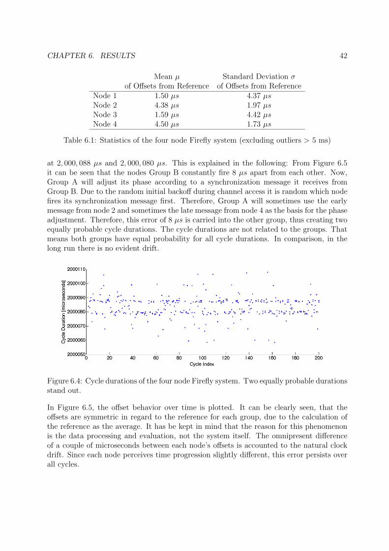
CHAPTER 6. RESULTS 42
Mean µ Standard Deviation σof Offsets from Reference of Offsets from Reference
Node 1 1.50 µs 4.37 µsNode 2 4.38 µs 1.97 µsNode 3 1.59 µs 4.42 µsNode 4 4.50 µs 1.73 µs
Table 6.1: Statistics of the four node Firefly system (excluding outliers > 5 ms)
at 2, 000, 088 µs and 2, 000, 080 µs. This is explained in the following: From Figure 6.5it can be seen that the nodes Group B constantly fire 8 µs apart from each other. Now,Group A will adjust its phase according to a synchronization message it receives fromGroup B. Due to the random initial backoff during channel access it is random which nodefires its synchronization message first. Therefore, Group A will sometimes use the earlymessage from node 2 and sometimes the late message from node 4 as the basis for the phaseadjustment. Therefore, this error of 8 µs is carried into the other group, thus creating twoequally probable cycle durations. The cycle durations are not related to the groups. Thatmeans both groups have equal probability for all cycle durations. In comparison, in thelong run there is no evident drift.
Figure 6.4: Cycle durations of the four node Firefly system. Two equally probable durationsstand out.
In Figure 6.5, the offset behavior over time is plotted. It can be clearly seen, that theoffsets are symmetric in regard to the reference for each group, due to the calculation ofthe reference as the average. It has be kept in mind that the reason for this phenomenonis the data processing and evaluation, not the system itself. The omnipresent differenceof a couple of microseconds between each node’s offsets is accounted to the natural clockdrift. Since each node perceives time progression slightly different, this error persists overall cycles.
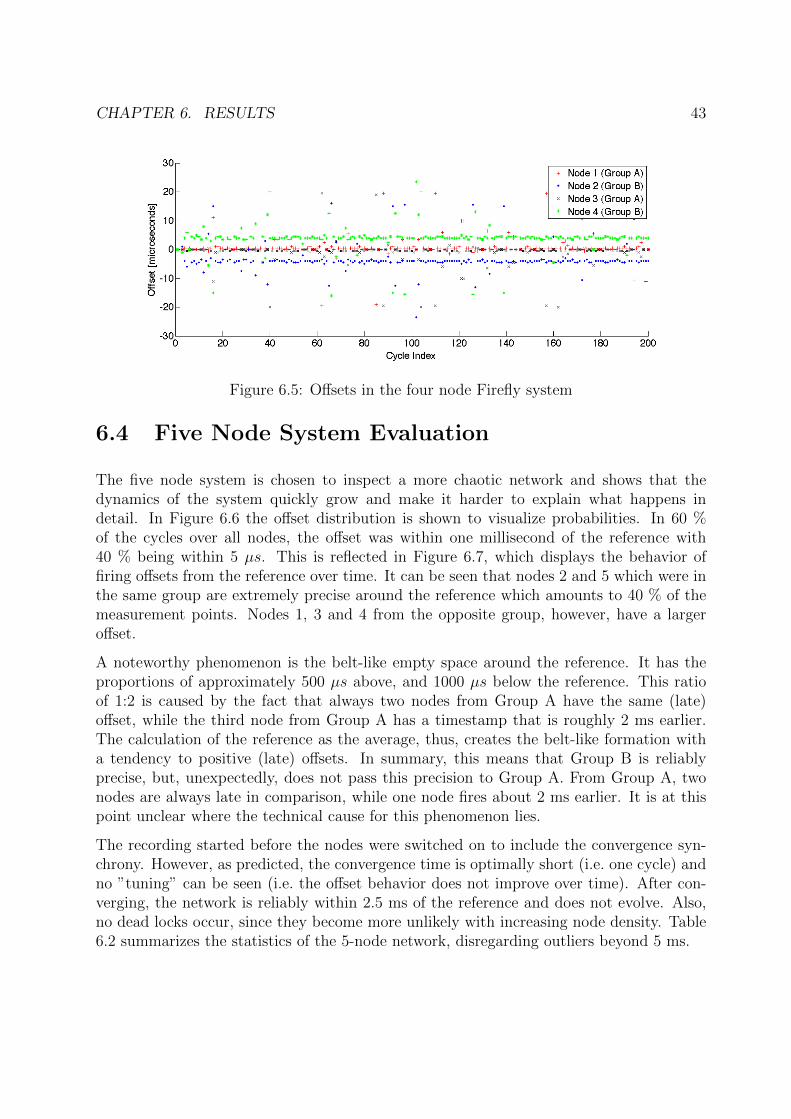
CHAPTER 6. RESULTS 43
Figure 6.5: Offsets in the four node Firefly system
6.4 Five Node System Evaluation
The five node system is chosen to inspect a more chaotic network and shows that thedynamics of the system quickly grow and make it harder to explain what happens indetail. In Figure 6.6 the offset distribution is shown to visualize probabilities. In 60 %of the cycles over all nodes, the offset was within one millisecond of the reference with40 % being within 5 µs. This is reflected in Figure 6.7, which displays the behavior offiring offsets from the reference over time. It can be seen that nodes 2 and 5 which were inthe same group are extremely precise around the reference which amounts to 40 % of themeasurement points. Nodes 1, 3 and 4 from the opposite group, however, have a largeroffset.
A noteworthy phenomenon is the belt-like empty space around the reference. It has theproportions of approximately 500 µs above, and 1000 µs below the reference. This ratioof 1:2 is caused by the fact that always two nodes from Group A have the same (late)offset, while the third node from Group A has a timestamp that is roughly 2 ms earlier.The calculation of the reference as the average, thus, creates the belt-like formation witha tendency to positive (late) offsets. In summary, this means that Group B is reliablyprecise, but, unexpectedly, does not pass this precision to Group A. From Group A, twonodes are always late in comparison, while one node fires about 2 ms earlier. It is at thispoint unclear where the technical cause for this phenomenon lies.
The recording started before the nodes were switched on to include the convergence syn-chrony. However, as predicted, the convergence time is optimally short (i.e. one cycle) andno ”tuning” can be seen (i.e. the offset behavior does not improve over time). After con-verging, the network is reliably within 2.5 ms of the reference and does not evolve. Also,no dead locks occur, since they become more unlikely with increasing node density. Table6.2 summarizes the statistics of the 5-node network, disregarding outliers beyond 5 ms.
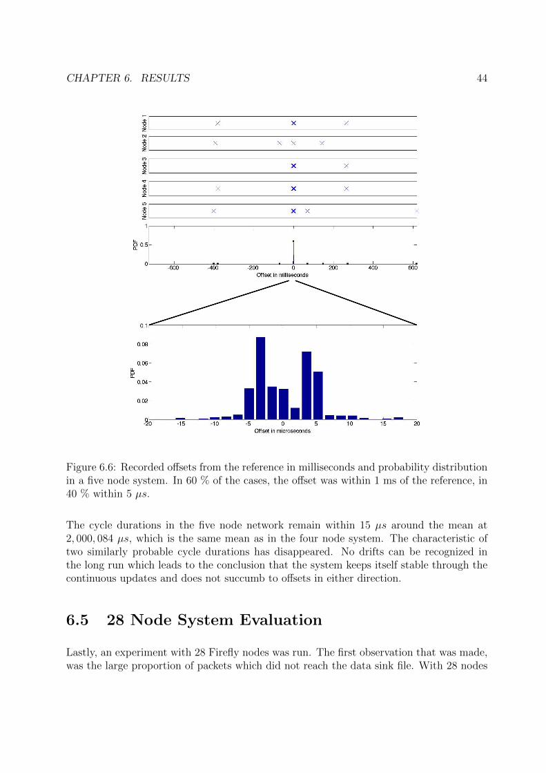
CHAPTER 6. RESULTS 44
Figure 6.6: Recorded offsets from the reference in milliseconds and probability distributionin a five node system. In 60 % of the cases, the offset was within 1 ms of the reference, in40 % within 5 µs.
The cycle durations in the five node network remain within 15 µs around the mean at2, 000, 084 µs, which is the same mean as in the four node system. The characteristic oftwo similarly probable cycle durations has disappeared. No drifts can be recognized inthe long run which leads to the conclusion that the system keeps itself stable through thecontinuous updates and does not succumb to offsets in either direction.
6.5 28 Node System Evaluation
Lastly, an experiment with 28 Firefly nodes was run. The first observation that was made,was the large proportion of packets which did not reach the data sink file. With 28 nodes
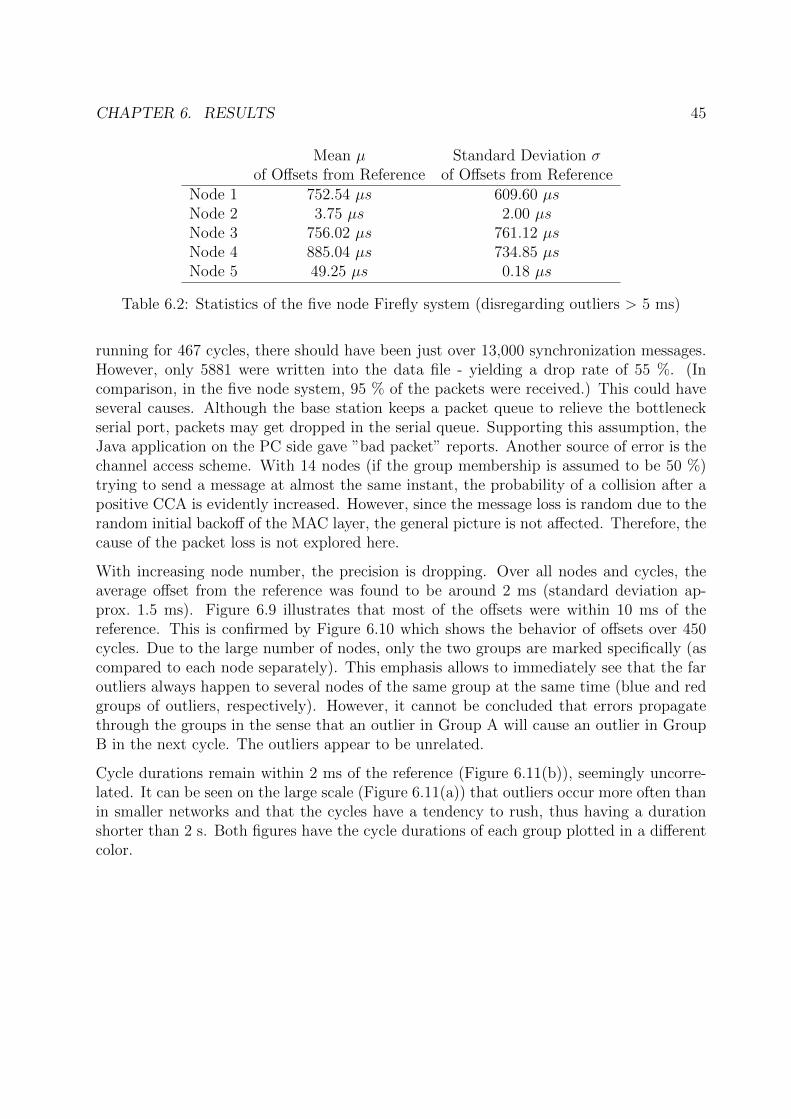
CHAPTER 6. RESULTS 45
Mean µ Standard Deviation σof Offsets from Reference of Offsets from Reference
Node 1 752.54 µs 609.60 µsNode 2 3.75 µs 2.00 µsNode 3 756.02 µs 761.12 µsNode 4 885.04 µs 734.85 µsNode 5 49.25 µs 0.18 µs
Table 6.2: Statistics of the five node Firefly system (disregarding outliers > 5 ms)
running for 467 cycles, there should have been just over 13,000 synchronization messages.However, only 5881 were written into the data file - yielding a drop rate of 55 %. (Incomparison, in the five node system, 95 % of the packets were received.) This could haveseveral causes. Although the base station keeps a packet queue to relieve the bottleneckserial port, packets may get dropped in the serial queue. Supporting this assumption, theJava application on the PC side gave ”bad packet” reports. Another source of error is thechannel access scheme. With 14 nodes (if the group membership is assumed to be 50 %)trying to send a message at almost the same instant, the probability of a collision after apositive CCA is evidently increased. However, since the message loss is random due to therandom initial backoff of the MAC layer, the general picture is not affected. Therefore, thecause of the packet loss is not explored here.
With increasing node number, the precision is dropping. Over all nodes and cycles, theaverage offset from the reference was found to be around 2 ms (standard deviation ap-prox. 1.5 ms). Figure 6.9 illustrates that most of the offsets were within 10 ms of thereference. This is confirmed by Figure 6.10 which shows the behavior of offsets over 450cycles. Due to the large number of nodes, only the two groups are marked specifically (ascompared to each node separately). This emphasis allows to immediately see that the faroutliers always happen to several nodes of the same group at the same time (blue and redgroups of outliers, respectively). However, it cannot be concluded that errors propagatethrough the groups in the sense that an outlier in Group A will cause an outlier in GroupB in the next cycle. The outliers appear to be unrelated.
Cycle durations remain within 2 ms of the reference (Figure 6.11(b)), seemingly uncorre-lated. It can be seen on the large scale (Figure 6.11(a)) that outliers occur more often thanin smaller networks and that the cycles have a tendency to rush, thus having a durationshorter than 2 s. Both figures have the cycle durations of each group plotted in a differentcolor.
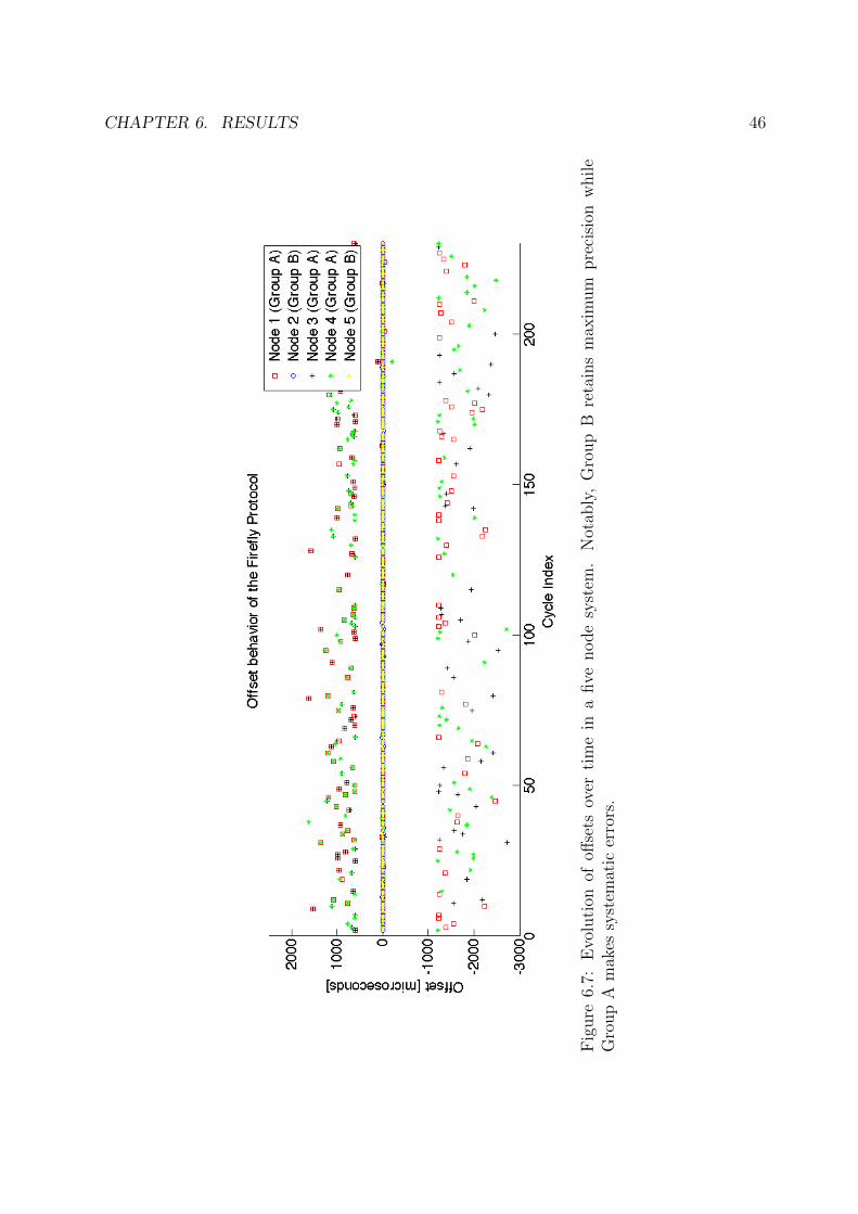
CHAPTER 6. RESULTS 46
Fig
ure
6.7:
Evo
luti
onof
offse
tsov
erti
me
ina
five
node
syst
em.
Not
ably
,G
roup
Bre
tain
sm
axim
um
pre
cisi
onw
hil
eG
roup
Am
akes
syst
emat
icer
rors
.
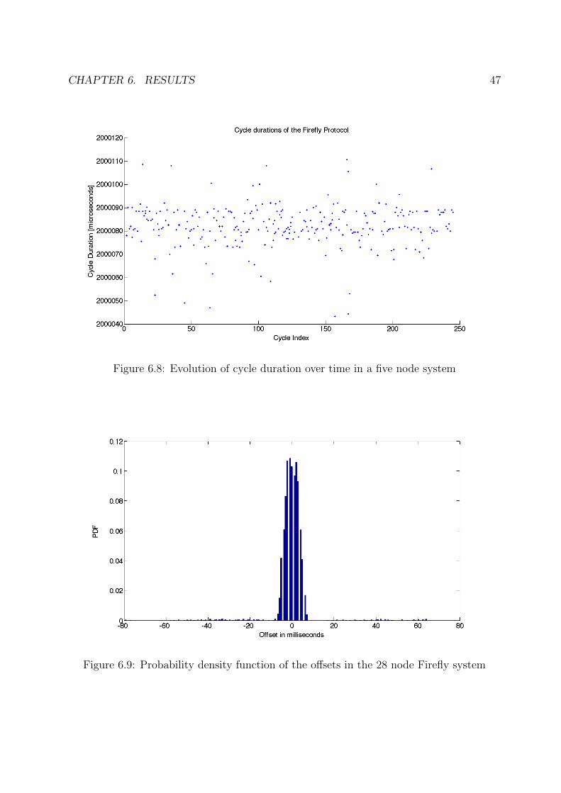
CHAPTER 6. RESULTS 47
Figure 6.8: Evolution of cycle duration over time in a five node system
Figure 6.9: Probability density function of the offsets in the 28 node Firefly system
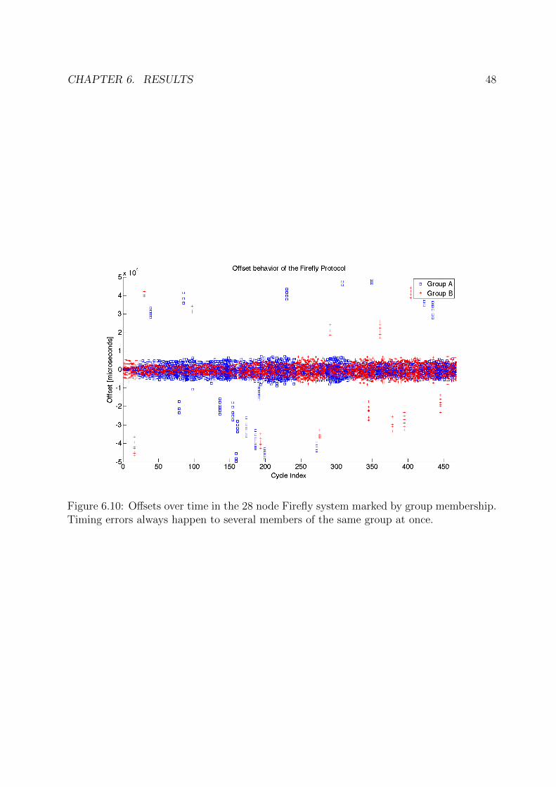
CHAPTER 6. RESULTS 48
Figure 6.10: Offsets over time in the 28 node Firefly system marked by group membership.Timing errors always happen to several members of the same group at once.
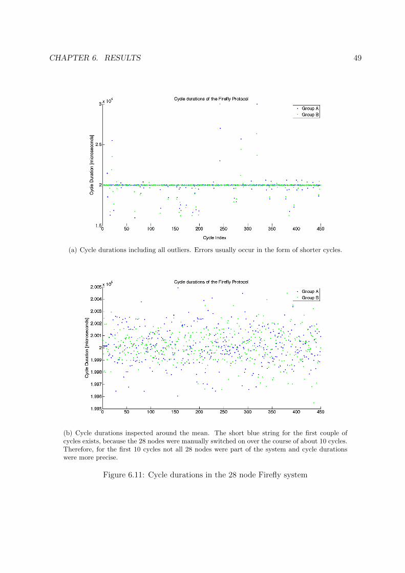
CHAPTER 6. RESULTS 49
(a) Cycle durations including all outliers. Errors usually occur in the form of shorter cycles.
(b) Cycle durations inspected around the mean. The short blue string for the first couple ofcycles exists, because the 28 nodes were manually switched on over the course of about 10 cycles.Therefore, for the first 10 cycles not all 28 nodes were part of the system and cycle durationswere more precise.
Figure 6.11: Cycle durations in the 28 node Firefly system
Chapter 7
Summary and Outlook
In this thesis, the biologically inspired Firefly Protocol (as suggested by Tyrrell et al. (19))is implemented on MICAz network nodes in TinyOS 2.0. The Firefly Protocol by Tyrrellet al., as well as the ”Firefly 2.0” Protocol implemented in this thesis, leave the traditionalhierarchical approach in synchronization behind and stride to enable a synchronized net-work of equal nodes. All synchronization protocols that have been implemented so far haveused notions of hierarchy (either static or elected) to clarify the source of reference timein a network (11; 18; 12). The Firefly approach drops this necessity by allowing nodes toreach a consensus as pulse-coupled oscillators. After the system had been implemented, ithas been tested on networks consisting of 1, 2, 4, 5 and 28 nodes.
Several adjustments were necessary to apply the theoretical model in practice: The as-sumption of a constant and predictable transmit time in network nodes does not hold dueto internal non-deterministic delays. In addition, the wireless channel requires an accessscheme which was not considered in the model. Both of these delays sources can onlybe compensated a posteriori by the receiver of a synchronization message through knowl-edge of timestamps, which are created at message creation, transmission and reception.To reach microsecond precision it is necessary to methodically a) compensate for all non-deterministic and b) predict all deterministic delay sources in the system. In addition, thisthesis proposes a solution to the dead lock situation which can occur in a sparse Fireflynetwork.
Nodes were found to make mistakes creating large offsets up to 400 ms, and thus, as aneffect of the consensus system, irritating the network as a whole. Therefore, the precisionof the entire network is of the order of 300 µs for five nodes and 2 ms for 28 nodes.However, in a single hop four node network individual nodes can reach up to 1.5 µs averageoffset. Therefore, in matters of precision, this protocol is in the range of the hierarchicalapproaches. Yet, it remains to be tested over multiple hops. In the current setting, theprotocol is not consistent enough, to allow for longer cycle durations which are necessaryfor better energy efficiency. In regard to the other synchronization protocols which were
50
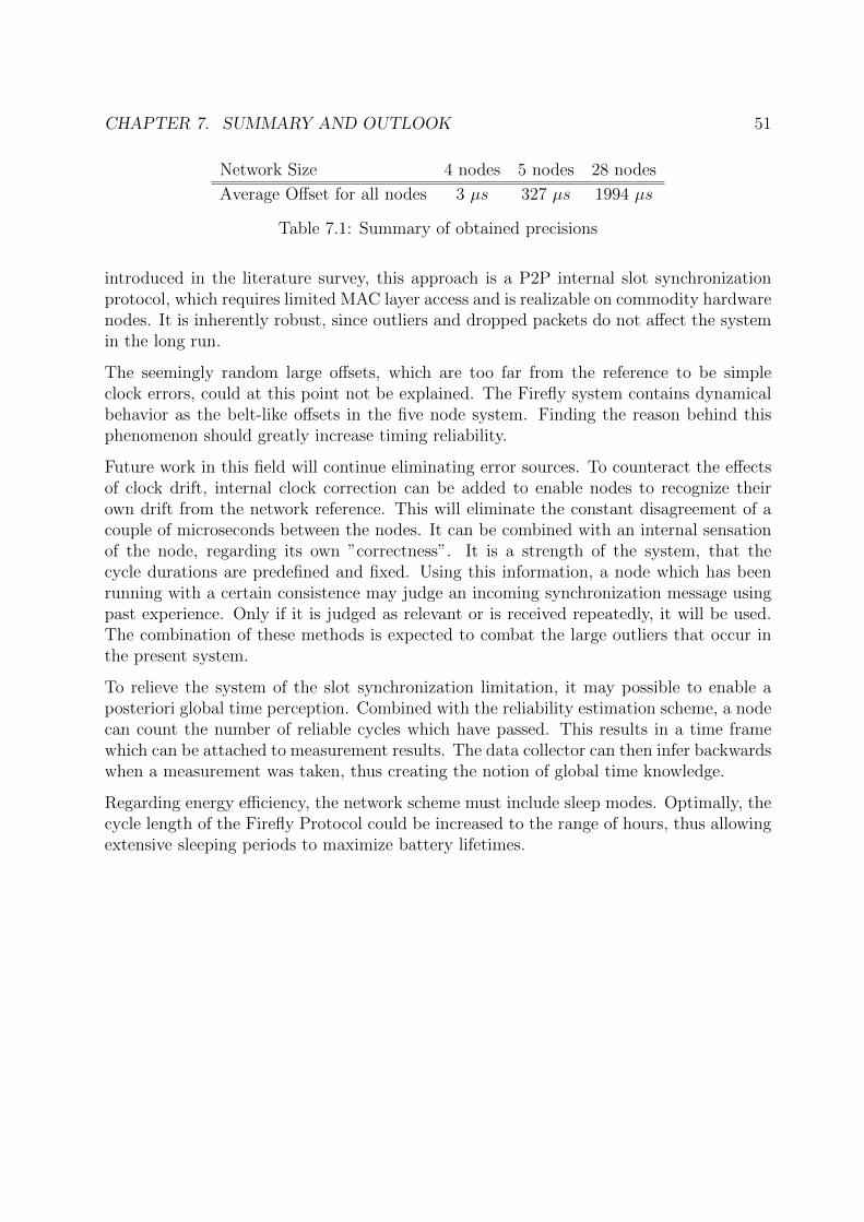
CHAPTER 7. SUMMARY AND OUTLOOK 51
Network Size 4 nodes 5 nodes 28 nodes
Average Offset for all nodes 3 µs 327 µs 1994 µs
Table 7.1: Summary of obtained precisions
introduced in the literature survey, this approach is a P2P internal slot synchronizationprotocol, which requires limited MAC layer access and is realizable on commodity hardwarenodes. It is inherently robust, since outliers and dropped packets do not affect the systemin the long run.
The seemingly random large offsets, which are too far from the reference to be simpleclock errors, could at this point not be explained. The Firefly system contains dynamicalbehavior as the belt-like offsets in the five node system. Finding the reason behind thisphenomenon should greatly increase timing reliability.
Future work in this field will continue eliminating error sources. To counteract the effectsof clock drift, internal clock correction can be added to enable nodes to recognize theirown drift from the network reference. This will eliminate the constant disagreement of acouple of microseconds between the nodes. It can be combined with an internal sensationof the node, regarding its own ”correctness”. It is a strength of the system, that thecycle durations are predefined and fixed. Using this information, a node which has beenrunning with a certain consistence may judge an incoming synchronization message usingpast experience. Only if it is judged as relevant or is received repeatedly, it will be used.The combination of these methods is expected to combat the large outliers that occur inthe present system.
To relieve the system of the slot synchronization limitation, it may possible to enable aposteriori global time perception. Combined with the reliability estimation scheme, a nodecan count the number of reliable cycles which have passed. This results in a time framewhich can be attached to measurement results. The data collector can then infer backwardswhen a measurement was taken, thus creating the notion of global time knowledge.
Regarding energy efficiency, the network scheme must include sleep modes. Optimally, thecycle length of the Firefly Protocol could be increased to the range of hours, thus allowingextensive sleeping periods to maximize battery lifetimes.
Appendix A
Appendix
A.1 Tools
At many points during this work, it was necessary to check, evaluate or measure com-ponents of a node or the entire system. For this purpose, various test applications werecreated which are shortly mentioned here and can be found on the accompanying CD.
A.1.1 BaseStation
The BaseStation component was the data collector for the Firefly network. The standardBaseStation which is provided with TinyOS was modified to have an increased messagebuffer. All incoming radio messages are timestamped and passed to the serial port.
A.1.2 BSJitterSerial
The original base station jitter measurement component was used to measure radio sendinghardware delays and medium access delays. It was extended over the course of the projectto perform outgoing and incoming message timestamps, AM ID-dependent timestampsand shut-off of CCA. Later it was the basis for the round trip measurement system asdescribed in Section 4.2.2.
A.1.3 LabSync
LabSync was the most basic approach to a firefly system and was designed as a problemsubmission for the wireless sensor laboratory. Operating in the millisecond range, LabSyncallows to blink LEDs synchronously.
52
APPENDIX A. APPENDIX 53
A.1.4 ReadTime
The RadioTimeStamping interface was explored in the ReadTime component. As describedin Section 4.2.2, the 8-bit counter was found to be too narrow.
A.1.5 TimerCheck
The TimerCheck component was used to compare the different timers that are available onMICAz. By starting, stopping and restarting various timers repeatedly, hardware delaysand timer reliability were explored.
A.1.6 TrafficSource
A mote which runs TrafficSource will continually send back-to-back messages. Each suc-cessful transmission of a dummy packet triggers the transmission of the next message. Itwas used to push the Contention Backoff of the CSMA scheme.
A.2 TinyOS Modules and Components Used
The most straightforward way to describe the components of the Firefly Protocol is toprint the contents of the configuration file. All components and wirings used are listedbelow:
// Main component
components FireflyC as App;
components MainC;
App.Boot -> MainC;
// LED control
components LedsC;
App.Leds -> LedsC;
// Random number generator (used in the dead lock circumvention)
components RandomC;
App.Random -> RandomC;
// Timers
components CounterMicro32C as Counter32;
App.Counter -> Counter32;
APPENDIX A. APPENDIX 54
components new AlarmMicro32C() as Alarm32;
App.Alarm -> Alarm32;
// ActiveMessageRadio
components ActiveMessageC as AM;
App.RadioControl -> AM;
App.RadioPacket -> AM;
App.SyncSend -> AM.AMSend[AM_FIREFLY_SYNC_MSG];
App.SyncReceive -> AM.Receive[AM_FIREFLY_SYNC_MSG];
// Radio chip control interface - used for timestamping
components CC2420TransmitC;
App.RadioTimeStamping -> CC2420TransmitC;
App.CC2420Transmit -> CC2420TransmitC;
// Optional interface for backoff modification and CCA control
components CC2420CsmaC;
App.RadioBackoff -> CC2420CsmaC.RadioBackoff[AM_FIREFLY_SYNC_MSG];
A.3 Errors
Node Lock-up
There exists an error where the network node software freezes. The frozen node will remainwith one LED switched on and not be susceptible to incoming messages. It is assumedthat this problem is caused by the message receive interrupt. While one synchronizationmessage is still being processed and states are about to change, the next message interruptis triggered, thus stopping the state change and locking the node. This error has not beeninvestigated further as it can be easily recognized in the laboratory and fixed through areboot. It becomes more probable with growing network size and has been not encounteredwith less than 5 nodes. The probability of this error is roughly estimated at 1 lock-up per5,000 synchronization messages (e.g. 10 nodes going through 500 cycles will probably causeone lock-up).
List of Figures
2.1 From Production Price to Overhead . . . . . . . . . . . . . . . . . . . . . . 9
3.1 Pteroptyx Mallaccae (Source: www.rspg.org) . . . . . . . . . . . . . . . . . . 173.2 The Firefly’s flashing phases . . . . . . . . . . . . . . . . . . . . . . . . . . 183.3 Time evolution of the phase function in the Firefly Protocol (23) . . . . . . 193.4 Phase diagram for an oscillator by Tyrrell et al. Two groups of oscillators
form, spaced T apart. . . . . . . . . . . . . . . . . . . . . . . . . . . . . . . 213.5 Delay estimates for an idealized point of a message . . . . . . . . . . . . . 233.6 Timestamping of the Firefly 2.0 protocol in detail . . . . . . . . . . . . . . 26
4.1 The MICAz network node (Source: www.xbow.com) . . . . . . . . . . . . . 294.2 Measurement setup for perceived timings in network nodes . . . . . . . . . 314.3 CSMA Characterization . . . . . . . . . . . . . . . . . . . . . . . . . . . . 33
5.1 Laboratory setup for the evaluation of the Firefly Protocol (simplified) . . 36
6.1 Single Node Cycle Duration . . . . . . . . . . . . . . . . . . . . . . . . . . 396.2 Evaluation of the two node Firefly system . . . . . . . . . . . . . . . . . . 406.3 Offset values and distribution of the four node Firefly system . . . . . . . . 416.4 Cycle durations of the four node Firefly system . . . . . . . . . . . . . . . 426.5 Offsets in the four node Firefly system . . . . . . . . . . . . . . . . . . . . 436.6 Offsets in the five node system . . . . . . . . . . . . . . . . . . . . . . . . . 446.7 Evolution of offsets over time in a five node system . . . . . . . . . . . . . 466.8 Evolution of cycle duration over time in a five node system . . . . . . . . . 476.9 Probability density function of the offsets in the 28 node Firefly system . . 476.10 Offsets over time in the 28 node Firefly system . . . . . . . . . . . . . . . . 486.11 Cycle durations in the 28 node Firefly system . . . . . . . . . . . . . . . . 49
55
List of Tables
2.1 Comparison of Synchronization Protocols . . . . . . . . . . . . . . . . . . . 15
3.1 State durations used in this work . . . . . . . . . . . . . . . . . . . . . . . 22
4.1 MICAz hardware parameters . . . . . . . . . . . . . . . . . . . . . . . . . . 284.2 Available timer precisions in TinyOS/MICAz . . . . . . . . . . . . . . . . 304.3 Results of the internal clock comparison in MICAz motes . . . . . . . . . . 31
6.1 Statistics of the four node Firefly system (excluding outliers > 5 ms) . . . 426.2 Statistics of the five node Firefly system (disregarding outliers > 5 ms) . . 45
7.1 Summary of obtained precisions . . . . . . . . . . . . . . . . . . . . . . . . 51
56
Bibliography
[1] Ian Akyildiz and Weilian Su. A survey on sensor networks. IEEE CommunicationsMagazine, 13:102–114, 2002.
[2] Ivan Stojmenovic. Handbook of Sensor Networks. Wiley Interscience, 2005.
[3] Kay Roemer. Time Synchronization and Localization in Sensor Networks. Ph.D.thesis, Swiss Federal Institute of Technology Zurich, 2005.
[4] Pritvish Basu and Thomas Little. Networked parking spaces: architecture and ap-plications. Proceedings of the 56th Vehicular Technology Conference, 2:1153 – 1157,2002.
[5] Gyula Simon, Miklos Maroti, Akos Ledeczi, Gyorgy Balogh, Branislav Kusy, AndrasNadas, Gabor Pap, Janos Sallai, and Ken Frampton. Sensor network-based coun-tersniper system. In SenSys ’04: Proceedings of the 2nd international conference onEmbedded networked sensor systems, pages 1–12. ACM, New York, NY, USA, 2004.ISBN 1-58113-879-2. doi:http://doi.acm.org/10.1145/1031495.1031497.
[6] B. Sundaraman, Ugo Buy, and Ajay Kshemkalyani. Clock Synchronization for WirelessSensor Networks: A Survey. Master’s thesis, University of Illinois at Chicago, 2005.
[7] Fikret Sivrikaya and Bulent Yener. Time synchronization in sensor networks: A survey.IEEE Network, 18:45 – 50, 2004.
[8] Holger Karl and Andreas Willig. Protocols and Architectures for Wireless SensorNetworks. John Wiley & Sons, 2005.
[9] David Mills. Internet time synchronization: The internet time protocol. IEEE Trans-actions on Communications, 39:1482–1493, 1991.
[10] David Mills. Improved algorithms for synchronizing computer network clocks.IEEE/ACM Transactions on Networking, 3:245 – 254, 1995.
[11] Jeremy Elson, Deborah Estrin, and Lewis Girod. Fine-grained network time syn-chronization using reference broadcasts. In Proceedings of the Fifth Symposium onOperating Systems Design and Implementation. 2002.
57
BIBLIOGRAPHY 58
[12] Miklos Maroti and Branislav Kusy. The flooding time synchronization protocol. InProceedings of the 2nd international conference on Embedded networked sensor sys-tems, pages 39 – 49. 2004.
[13] Ian Akyildiz and Weilian Su. Time-diffusion synchronization protocol for wirelesssensor networks. IEEE Transactions on Networking, 13:384–397, 2005.
[14] Qun Li and Daniela Rus. Global clock synchronization in sensor networks. IEEETransactions on Computers, 55:214 – 226, 2006.
[15] Jang-Ping Sheu and Chih-Min Chao. A clock synchronization algorithm for multi-hop wireless ad hoc networks. Wireless Personal Communications: An InternationalJournal, 43:185 – 200, 2007.
[16] Hui Dai and Richard Han. Tsync: A lightweicht bidirectional time synchronizationservice for wireless sensor networks. Mobile Computing and Communications Review,8:125 – 139, 2003.
[17] Kay Roemer. Time and location in sensor networks. In Proc. GI/ITG Workshop onSensor Networks, pages 57–60. 2003.
[18] Saurabh Ganeriwal and Ram Kumar. Timing-sync protocol for sensor networks. InProceedings of the 1st international conference on Embedded networked sensor systems.2003.
[19] Alexander Tyrrell, Gunther Auer, and Christian Bettstetter. Fireflies as role modelsfor synchronization in ad hoc networks. In 1st Conference on Bio-Inspired Models ofNetwork, Information and Computing Systems. 2006.
[20] Yao-Win Hong and Anna Scaglione. A scalable synchronization protocol for largescale sensor networks and its applications. IEEE Journal on Selected Areas in Com-munications, 23:1085–1099, 2005.
[21] R. Mirollo and S. Strogatz. Synchronization of pulse-coupled biological oscillators.SIAM J. Appl. Math, 50:1645–1662, 1990.
[22] An-Swol Hu and Sergio Servetto. Algorithmisc aspects of the time synchronizationproblem in large-scale sensor networks. Mobile Networks and Applications, 10:491–503,2005.
[23] Alexander Tyrrell, Gunther Auer, and Christian Bettstetter. Synchronization inspiredfrom nature for wireless meshed networks. International Conference on Wireless Com-munications, Networking and Mobile Computing, 1:1 – 4, 2006.
[24] John Buck, Elisabeth Buck, and James Case. Control of flashing in fireflies. pacemakersynchronization in pteroptyx cribellata. Journal of Comparative Physiology, 144:630– 633, 1981.
BIBLIOGRAPHY 59
[25] Daniel Otte. Synchrony in texas fireflies with a consideration of male interactionmodels. Biology of Behaviour, 2:143–158, 1977.
[26] John Jalife. Mutual entrainment and electrical coupling as mechanisms for syn-chronous firing of rabbit sino-atrial pace-maker cells. Journal of Physiology, 356:221– 243, 1984.
[27] Thomas Walker. Acoustic synchrony: Two mechanisms in the snowy tree cricket.Science, 166:891–894, 1969.
[28] Martin McClintock. Menstrual synchrony and suppression. Nature, 229:244 – 245,1971.
[29] Charles Peskin. Mathematical Aspects of Heart Physiology. Courant Institute of Math-ematical Sciences, 1975.
[30] An-Swol Hu and Sergio Servetto. Asymptotically optimal time synchronization indense sensor networks. Proceedings of the 2nd ACM international conference on Wire-less sensor networks and applications, 1:1 – 10, 2003.
[31] Dennis Lucarelli and Jeng Wang. Decentralized synchronization protocols with near-est neighbor communication. In Proceedings of the 2nd International Conference onEmbedded Networked Sensor Systems. 2004.
[32] Yao-Win Hong and Anna Scaglione. Time synchronization and reach-back commu-nications with pulse-coupled oscillators for uwb wireless ad hoc networks. In IEEEConference on Ultra Wideband Systems and Technologies. 2003.
[33] Philip Levis and Nelson Lee. Tossim: accurate and scalable simulation of entire tinyosapplications. In Proceedings of the 1st international conference on Embedded networkedsensor systems. 2003.
[34] Andrew S. Tanenbaum. Computer networks: 2nd edition. Prentice-Hall, Inc., UpperSaddle River, NJ, USA, 1988. ISBN 0-13-162959-X.
[35] Anis Koubaa and Mario Alves. A comprehensive simulation study of slotted csma/cafor ieee 802.15.4 wireless sensor networks. In IEEE International Workshop on FactoryCommunication Systems. 2006.
[36] G. J. Pottie and W. J. Kaiser. Wireless integrated network sensors. Commun. ACM,43(5):51–58, 2000. ISSN 0001-0782. doi:http://doi.acm.org/10.1145/332833.332838.
Related Documents