J. Fluid Mech. (2005), vol. 522, pp. 1–33. c 2005 Cambridge University Press DOI: 10.1017/S002211200400120X Printed in the United Kingdom 1 Decaying grid turbulence in a strongly stratified fluid By OLIVIER PRAUD, ADAM M. FINCHAM† AND JOEL SOMMERIA Laboratoire des Ecoulements G´ eophysiques et Industriels (LEGI) CNRS-UJF-INPG, Coriolis, BP53, 38041 Grenoble, cedex9, France (Received 5 September 2002 and in revised form 15 June 2004) Grid turbulence experiments have been carried out in a stably stratified fluid at moderately large Reynolds numbers (160 based on the Taylor microscale). A scanning particle image velocimetry technique is used to provide time-resolved velocity fields in a relatively large volume. For late times, in the low-Froude-number regime, the flow consists of quasi-horizontal motion in a sea of weak internal gravity waves. Here the dynamics of the flow is found to be independent of the ambient stratification. Fundamental differences with two-dimensional turbulence, due to the strong vertical shearing of horizontal velocity, are observed. In this regime, a self-similar scaling law for the energy decay and the length-scale evolution is observed. This behaviour reflects a process of adjustment of the eddy aspect ratio based on a balance between the horizontal advective motion which tends to vertically decorrelate the flow and the dissipation due to strong vertical shear. The characteristic vertical size of the eddies grows according to a diffusion law and is found to be independent of the turbulence generation. The organization of the flow into horizontal layers of eddies separated by intense shear leads to a strong anisotropy of the dissipation: this has been checked by direct measurement of the different tensorial components of the viscous dissipation. 1. Introduction The dynamical evolution of freely evolving turbulence in the presence of stable stratification is of great importance to the understanding of atmospheric and oceanic turbulence. The influence of stable density stratification on initially homogeneous three-dimensional turbulence has been studied by a number of workers. In one of the first experiments Dickey & Mellor (1980) dropped a biplane grid through a fluid at rest, and Britter et al. (1983) dragged a grid through a stratified fluid. They obtained interesting data concerning the decay rate of the vertical velocity. Britter et al. (1983) have shown that the main effect of the buoyancy forces is to suppress the vertical velocity component. Experiments were performed by Stillinger, Helland & Van Atta (1983) and Itsweire, Helland & Van Atta (1986) in a close loop channel, stratified with ten layers of salt water, and similar work was done later in a wind tunnel using stratified heated air by Lienhard & Van Atta (1990) and Yoon & Warhaft (1990). All these experiments have characterized the initial collapse of the three-dimensional turbulence, the damping effect of the density stratification on turbulence, and the statistical properties of the flow at early time. † Address for correspondence: AME Department, USC, 854 W 36th Place, Los Angeles, CA 90089-1191, USA

Welcome message from author
This document is posted to help you gain knowledge. Please leave a comment to let me know what you think about it! Share it to your friends and learn new things together.
Transcript
J. Fluid Mech. (2005), vol. 522, pp. 1–33. c© 2005 Cambridge University Press
DOI: 10.1017/S002211200400120X Printed in the United Kingdom
1
Decaying grid turbulence in a stronglystratified fluid
By OLIVIER PRAUD, ADAM M. FINCHAM†AND JOEL SOMMERIA
Laboratoire des Ecoulements Geophysiques et Industriels (LEGI) CNRS-UJF-INPG,Coriolis, BP53, 38041 Grenoble, cedex9, France
(Received 5 September 2002 and in revised form 15 June 2004)
Grid turbulence experiments have been carried out in a stably stratified fluid atmoderately large Reynolds numbers (160 based on the Taylor microscale). A scanningparticle image velocimetry technique is used to provide time-resolved velocity fieldsin a relatively large volume. For late times, in the low-Froude-number regime, theflow consists of quasi-horizontal motion in a sea of weak internal gravity waves. Herethe dynamics of the flow is found to be independent of the ambient stratification.Fundamental differences with two-dimensional turbulence, due to the strong verticalshearing of horizontal velocity, are observed. In this regime, a self-similar scalinglaw for the energy decay and the length-scale evolution is observed. This behaviourreflects a process of adjustment of the eddy aspect ratio based on a balance betweenthe horizontal advective motion which tends to vertically decorrelate the flow and thedissipation due to strong vertical shear. The characteristic vertical size of the eddiesgrows according to a diffusion law and is found to be independent of the turbulencegeneration. The organization of the flow into horizontal layers of eddies separated byintense shear leads to a strong anisotropy of the dissipation: this has been checked bydirect measurement of the different tensorial components of the viscous dissipation.
1. IntroductionThe dynamical evolution of freely evolving turbulence in the presence of stable
stratification is of great importance to the understanding of atmospheric and oceanicturbulence. The influence of stable density stratification on initially homogeneousthree-dimensional turbulence has been studied by a number of workers. In one of thefirst experiments Dickey & Mellor (1980) dropped a biplane grid through a fluid atrest, and Britter et al. (1983) dragged a grid through a stratified fluid. They obtainedinteresting data concerning the decay rate of the vertical velocity. Britter et al. (1983)have shown that the main effect of the buoyancy forces is to suppress the verticalvelocity component. Experiments were performed by Stillinger, Helland & Van Atta(1983) and Itsweire, Helland & Van Atta (1986) in a close loop channel, stratifiedwith ten layers of salt water, and similar work was done later in a wind tunnel usingstratified heated air by Lienhard & Van Atta (1990) and Yoon & Warhaft (1990).All these experiments have characterized the initial collapse of the three-dimensionalturbulence, the damping effect of the density stratification on turbulence, and thestatistical properties of the flow at early time.
† Address for correspondence: AME Department, USC, 854 W 36th Place, Los Angeles,CA 90089-1191, USA
2 O. Praud, A. M. Fincham and J. Sommeria
As well as experiments, a number of three-dimensional numerical studies of forcedor decaying stratified homogeneous turbulence have been performed, within theBoussinesq approximation. Riley, Metcalfe & Weissman (1981), Herring & Metais(1989) and Metais & Herring (1989) have examined the vertical structure and thedistribution of energy between wave and vortical modes. In these works the collapseof the turbulence under the effect of stratification was found to affect both thedynamical properties of the flow and its structure. They observed a reduction ofenergy transfer and an inhibition of vertical scale growth.
After the collapse of the turbulence, the effect of stratification becomes dominantand the flow evolves in the low-Froude-number regime. It is this regime in which weare interested here. In this regime, vertical displacement is inhibited by stratification,leaving only two possible modes of motion: internal waves and vortices withhorizontal motion. The flow is then characterized by a field of quasi-two-dimensionalvortices undulating in a sea of internal gravity waves (see Riley et al. 1981). Laboratoryexperiments on this stage of stratified turbulence (see Hopfinger 1987; Fincham,Maxworthy & Spedding 1996; Bonnier, Eiff & Bonneton 2000; de Rooij, Linden &Dalziel 1999) and numerical simulation (see Riley et al. 1981; Herring & Metais1989; Kimura & Herring 1996) have revealed that these vortices look like ‘pancakes’with a vertical extent thinner than the horizontal scale. A fine review of this stronglystratified limit can be found in Riley & Lelong (2000). In such a layered flow, energydissipation is associated with the strong vertical shear (see Riley et al. 1981; Herring &Metais 1989; Metais & Herring 1989; Fincham et al. 1996). This strong vertical shearis supposed to be responsible for the profound difference observed between two-dimensional turbulence and the late stages of stratified turbulence. However, themechanism of layering is still unclear, and the selection and the evolution of verticallength scale also remain an open question. Experiments where no vertical scale isinitially imposed (see Park, Whitehead & Gnanadeskian 1994; Fincham et al. 1996;Billant & Chomaz 2000a) show that layers can spontaneously emerge from two-dimensional horizontal flow.
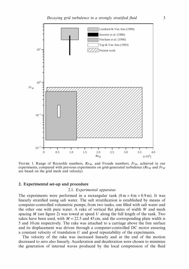
In the present paper, we study this low-Froude-number regime at higher Reynoldsnumbers than in previous studies, thanks to the large size of the facility. This allowsto get one step closer to the ideal inertial regimes typical of the ocean and theatmosphere. A Reynolds number of 160 is reached based on the vertical Taylormicroscale (36 000 based on grid mesh and velocity), while the Froude number issmaller than 0.6. Our parameters are compared in figure 1 with previous studies ofgrid-generated turbulence in a stratified fluid.
The main objectives of this work are to characterize the decay of stratifiedturbulence and to study the role of coherent structures in this regime. We willshow the profound differences that exist between this quasi-horizontal turbulence andpurely two-dimensional turbulence. The organization of the flow into staggered layersof quasi-horizontal motion leads to a strong anisotropy of the dissipation processthat will be described and quantified.
The paper is organized as follows. The experimental set-up and procedure arepresented in § 2. A general description of the flow is proposed in § 3, including thethree-dimensional structure, the energy decay and the evolution of the horizontaland vertical length scales. The spectral analysis of the flow is presented in § 4. In § 5we consider the contribution of the internal waves to the fluid motion by splittingthe velocity field into its vortical and wave parts. Finally, anisotropy and dissipationprocesses are discussed and quantified in § 6.
Decaying grid turbulence in a strongly stratified fluid 3
101
100
10–1
10–2
0 0.5 1.0 1.5 2.0 2.5 3.0 3.5 4.0ReM (×104)
Lienhard & Van Atta (1990)
Itsweire et al. (1986)
Fincham et al. (1996)
Yap & Van Atta (1993)
Present work
FrM
Figure 1. Range of Reynolds numbers, ReM , and Froude numbers, FrM , achieved in ourexperiments, compared with previous experiments on grid-generated turbulence (ReM and FrM
are based on the grid mesh and velocity).
2. Experimental set-up and procedure2.1. Experimental apparatus
The experiments were performed in a rectangular tank (8 m × 4 m × 0.9 m). It waslinearly stratified using salt water. The salt stratification is established by means ofcomputer-controlled volumetric pumps, from two tanks, one filled with salt water andthe other one with pure water. A rake of vertical flat plates of width W and meshspacing M (see figure 2) was towed at speed U along the full length of the tank. Tworakes have been used, with M =22.5 and 45 cm, and the corresponding plate width is5 and 10 cm respectively. The rake was attached to a carriage above the free surfaceand its displacement was driven through a computer-controlled DC motor ensuringa constant velocity of translation U and good repeatability of the experiments.
The velocity of the rake was increased linearly and at the end of the motiondecreased to zero also linearly. Acceleration and deceleration were chosen to minimizethe generation of internal waves produced by the local compression of the fluid
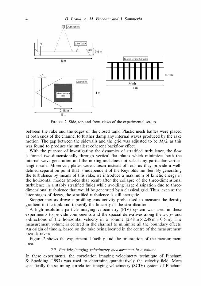
4 O. Praud, A. M. Fincham and J. Sommeria
U Laser sheet
CCD camera
ρ(z)
8 m
0.9 m
U
Measurementarea
Laser sheet
2.48 m8 m
4 m
4 mMesh
0.9 m
Rake of vertical flat plates
Figure 2. Side, top and front views of the experimental set-up.
between the rake and the edges of the closed tank. Plastic mesh baffles were placedat both ends of the channel to further damp any internal waves produced by the rakemotion. The gap between the sidewalls and the grid was adjusted to be M/2, as thiswas found to produce the smallest coherent backflow effect.
With the purpose of investigating the dynamics of stratified turbulence, the flowis forced two-dimensionally through vertical flat plates which minimizes both theinternal wave generation and the mixing and does not select any particular verticallength scale. Moreover, plates were chosen instead of rods as they provide a well-defined separation point that is independent of the Reynolds number. By generatingthe turbulence by means of this rake, we introduce a maximum of kinetic energy inthe horizontal modes (modes that result after the collapse of the three-dimensionalturbulence in a stably stratified fluid) while avoiding large dissipation due to three-dimensional turbulence that would be generated by a classical grid. Thus, even at thelater stages of decay, the stratified turbulence is still energetic.
Stepper motors drove a profiling conductivity probe used to measure the densitygradient in the tank and to verify the linearity of the stratification.
A high-resolution particle imaging velocimetry (PIV) system was used in theseexperiments to provide components and the spacial derivatives along the x-, y- andz-directions of the horizontal velocity in a volume (2.48 m × 2.48 m × 0.5 m). Themeasurement volume is centred in the channel to minimize all the boundary effects.An origin of time t0, based on the rake being located in the centre of the measurementarea, is taken.
Figure 2 shows the experimental facility and the orientation of the measurementarea.
2.2. Particle imaging velocimetry measurement in a volume
In these experiments, the correlation imaging velocimetry technique of Fincham& Spedding (1997) was used to determine quantitatively the velocity field. Morespecifically the scanning correlation imaging velocimetry (SCIV) system of Fincham
Decaying grid turbulence in a strongly stratified fluid 5
(1998) was used to explore its three-dimensional structure. The fluid was seeded with600 µm diameter polystyrene beads that were carefully prepared (by a process ofcooking, which decreases slightly the density and successive density separations)to have a flat distribution of densities matching that of the salt stratification.This process ensures that there are equal number densities of particles at eachdepth. A photographic surfactant (Ilfotol) was added to the working fluid is smallconcentrations to prevent the polystyrene beads from agglomerating. The particleconcentration must be sufficient to achieve good SCIV results but an excessive densityleads to a serious damping of laser light. We use a typical concentration of 0.02 particleper pixel. The corresponding volume concentration is about 10−4 g cm−3 which doesnot perturb the flow properties. We can also derive an estimate of the characteristictime, τs , needed for particles to attain velocity equilibrium with the fluid using Stockesdrag: τs = d2
pρp/18µ, where dp is the diameter and ρp the density of the tracer particlesand µ the dynamic viscosity. Using 600 µm diameter particles, the relaxation timeis about 0.02 s which is much shorter than the characteristic time scale of the flow.We can therefore consider that the particles passively follow the fluid motion.
Coherent light originating from an 8 W argon laser was passed into an optical fibrethe other end of which was attached to a small optical assembly which directs thelight onto a small oscillating mirror (Cambridge Technology model 6850) creatinga vertical light sheet. This small optical assembly moves horizontally on a linearbearing traverse. The light sheet then passes through a thin glass plate held parallelto and just touching the surface of the water above a 45 mirror placed in the water.In this way, horizontal motion of the optical assembly above the water translatesdirectly into vertical motion of the horizontal laser sheet within the fluid. Due to therefractive-index variation with depth, an initially horizontal beam of light will tendto curve downwards parabolically. In order to minimize this, only relatively weakstratifications were used and the angle of the horizontal light sheet was carefullyinclined upwards a few degrees such that the summit of its parabolic trajectorycorresponded to the centre of the measurement area. In this way the maximumdeviation from horizontal occurs at the edges of the images and is limited to about5 mm which is close to the light-sheet thickness.
The volume scanning process proceeded as follows: an initial scan through alldepths is made with continuous image acquisition to memory, the light sheet is quicklyreturned to the starting position, and after an appropriate time interval the scanprocess is repeated to acquire the second image in each pair. The images are acquiredby a 1024 × 1024 pixels 12-bit SMD 1M60 digital progressive scan camera operatingat 60 f.p.s., placed 4 m above the free surface. Each slice (corresponding to a pairof images) is treated as described by Fincham & Spedding (1997) and Fincham &Delerce (2000). This correlation imaging velocimetry (CIV) technique is based onthe calculation in physical space of the cross-correlation between local regions in thetwo images. The first image is divided into small rectangular boxes and the meandisplacement of a given box is determined from the location of the maximum of thecross-correlation function. In an iterative way, the deformation of the fluid withineach box is accounted for by locally deforming the images through use of a continuousfunction describing the discretely measured pixel intensities. As the true position ofeach velocity vector is located midway between the initial and final position of eachpattern box, the velocity field is then reinterpolated onto a rectangular Cartesiangrid using the thin-shell spline routines of Paihua (1978), as described in Spedding &Rignot (1993). The resulting two-dimensional vector fields are combined into a cubethat is fitted with a three-dimensional fourth-order tensor spline. Spatial derivatives
6 O. Praud, A. M. Fincham and J. Sommeria
along x, y and z are then computed analytically from the coefficients of the splinetensor. Typical measurement conditions produce 80 × 80 × 50 independent vectorsin a volume of 250 × 250 × 50 cm3. A combination of numerical simulations of thescanning technique, combined with actual hardware tests using real particles frozeninside a clear resin block, along with tests on stagnant fluid, showed that underoptimum conditions the measured mean r.m.s. error in velocity is less than 2%.
2.3. Scales and parameters
The relative importance of stratification is indicated by the Froude number,Fr = u/NL, where u is the r.m.s. turbulence velocity, L a length scale of the energy-containing motion and N =
√−g/ρo(∂ρ/∂z) the buoyancy frequency, ∂ρ/∂z is the
ambient density gradient and ρo the mean density. The Froude number is a measureof the relative importance of the buoyancy effects compared to the inertial forces. Inthe early time after the generation of turbulence some patches with relatively largeFroude number are found, suggesting the domination of the inertial effect. However,as the turbulence decays, the Froude number rapidly decreases as u decreases and L
tends to grow. As time goes on, and turbulence decays further, Fr becomes small andthe flow is completely dominated by stratification.
We define an initial Froude number, FrM , from the mesh size M , the grid velocityU and the Brunt–Vaisala frequency N , which are the main control parameters:
FrM =U
NM.
We similarly define the initial Reynolds number ReM :
ReM =UM
ν
where ν is the mean kinematic viscosity, i.e. the viscosity of the salt solution at mid-depth of the tank (viscosity varies by 5.6% with depth for the highest stratification).For a given stratification, ReM and FrM are related by ReM = FrMNM2/ν so that theFroude and Reynolds numbers vary together with U .
Experiments were performed for towing speeds U of 0.5, 1, 2, 4, 8 cm s−1 anddensity gradients with buoyancy frequencies N of 0.52 and 0.26 rad s−1. Two differentgrids were used: M = 45 cm and M = 22.5 cm. The corresponding Reynolds andFroude numbers are in the range 1125< ReM < 36 000 and 0.02 < FrM < 0.7. Table 1summarizes the parameters of the different experiments. The Reynolds number basedon the vertical Taylor microscale, Reλ = u∗λ∗
vReM = 0.85 Re1/2M , is also indicated.
Here the non-dimensional turbulent velocity u∗ and scale λ∗v are given from the
measurements respectively using (3.1) and (3.6). This Reynolds number slightlydecreases with time, and the data of table 1 are obtained with t∗ ≡ tU/M = 10,corresponding roughly to the beginning of the well-established turbulent decay.
3. General description3.1. Global decay of turbulence
Depending on the experimental parameters, two different initial behaviours areobserved. For low towing speeds, a laminar initial wake in which the motion remainstwo-dimensional and the vortices are initially columnar is observed. For higher towingspeeds, the flow behind the rake is initially fully turbulent but rapidly collapses underthe effect of stratification.
Decaying grid turbulence in a strongly stratified fluid 7
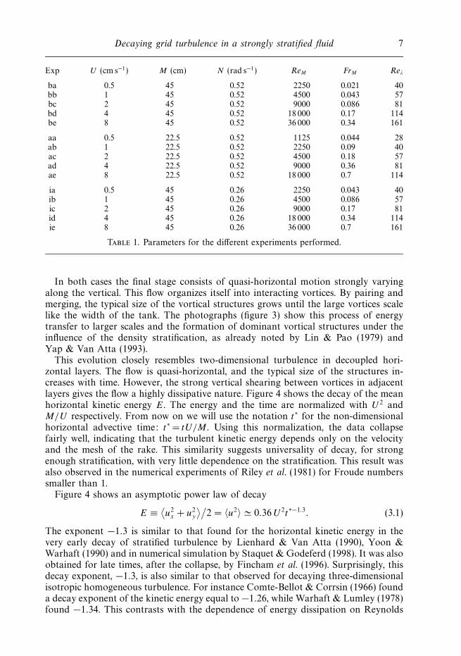
Exp U (cm s−1) M (cm) N (rad s−1) ReM FrM Reλ
ba 0.5 45 0.52 2250 0.021 40bb 1 45 0.52 4500 0.043 57bc 2 45 0.52 9000 0.086 81bd 4 45 0.52 18 000 0.17 114be 8 45 0.52 36 000 0.34 161
aa 0.5 22.5 0.52 1125 0.044 28ab 1 22.5 0.52 2250 0.09 40ac 2 22.5 0.52 4500 0.18 57ad 4 22.5 0.52 9000 0.36 81ae 8 22.5 0.52 18 000 0.7 114
ia 0.5 45 0.26 2250 0.043 40ib 1 45 0.26 4500 0.086 57ic 2 45 0.26 9000 0.17 81id 4 45 0.26 18 000 0.34 114ie 8 45 0.26 36 000 0.7 161
Table 1. Parameters for the different experiments performed.
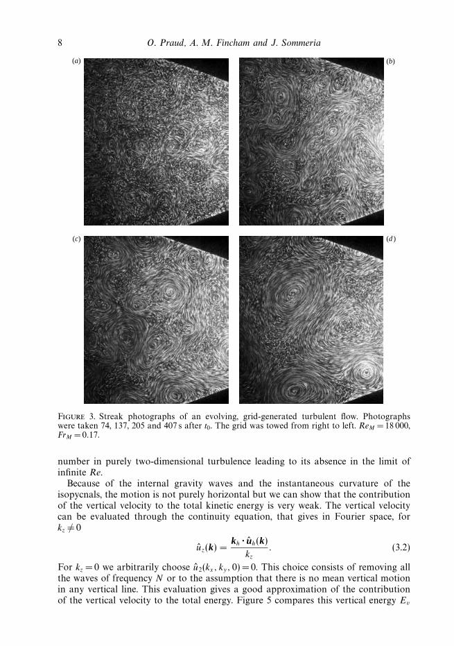
In both cases the final stage consists of quasi-horizontal motion strongly varyingalong the vertical. This flow organizes itself into interacting vortices. By pairing andmerging, the typical size of the vortical structures grows until the large vortices scalelike the width of the tank. The photographs (figure 3) show this process of energytransfer to larger scales and the formation of dominant vortical structures under theinfluence of the density stratification, as already noted by Lin & Pao (1979) andYap & Van Atta (1993).
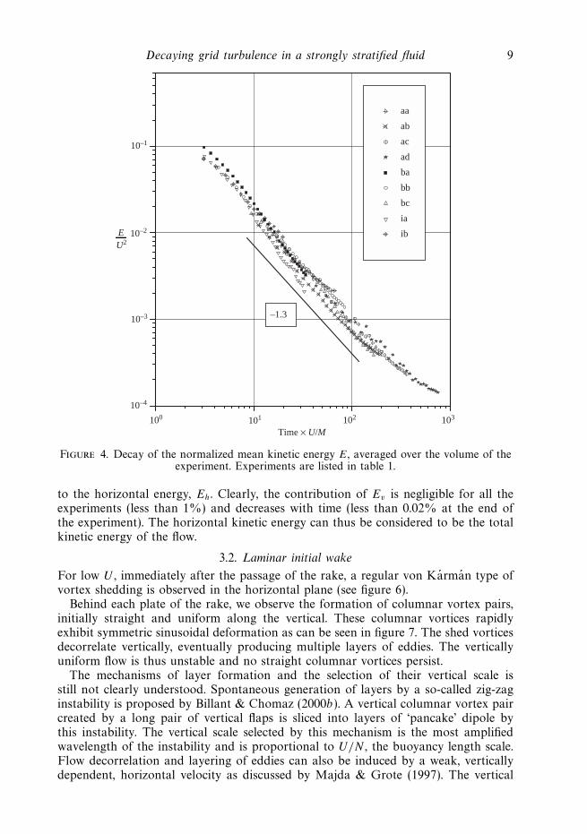
This evolution closely resembles two-dimensional turbulence in decoupled hori-zontal layers. The flow is quasi-horizontal, and the typical size of the structures in-creases with time. However, the strong vertical shearing between vortices in adjacentlayers gives the flow a highly dissipative nature. Figure 4 shows the decay of the meanhorizontal kinetic energy E. The energy and the time are normalized with U 2 andM/U respectively. From now on we will use the notation t∗ for the non-dimensionalhorizontal advective time: t∗ = tU/M . Using this normalization, the data collapsefairly well, indicating that the turbulent kinetic energy depends only on the velocityand the mesh of the rake. This similarity suggests universality of decay, for strongenough stratification, with very little dependence on the stratification. This result wasalso observed in the numerical experiments of Riley et al. (1981) for Froude numberssmaller than 1.
Figure 4 shows an asymptotic power law of decay
E ≡⟨u2
x + u2y
⟩/2 = 〈u2〉 0.36 U 2t∗−1.3. (3.1)
The exponent −1.3 is similar to that found for the horizontal kinetic energy in thevery early decay of stratified turbulence by Lienhard & Van Atta (1990), Yoon &Warhaft (1990) and in numerical simulation by Staquet & Godeferd (1998). It was alsoobtained for late times, after the collapse, by Fincham et al. (1996). Surprisingly, thisdecay exponent, −1.3, is also similar to that observed for decaying three-dimensionalisotropic homogeneous turbulence. For instance Comte-Bellot & Corrsin (1966) founda decay exponent of the kinetic energy equal to −1.26, while Warhaft & Lumley (1978)found −1.34. This contrasts with the dependence of energy dissipation on Reynolds
8 O. Praud, A. M. Fincham and J. Sommeria
(a)
(c) (d )
(b)
Figure 3. Streak photographs of an evolving, grid-generated turbulent flow. Photographswere taken 74, 137, 205 and 407 s after t0. The grid was towed from right to left. ReM =18 000,FrM = 0.17.
number in purely two-dimensional turbulence leading to its absence in the limit ofinfinite Re.
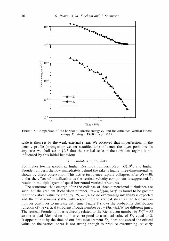
Because of the internal gravity waves and the instantaneous curvature of theisopycnals, the motion is not purely horizontal but we can show that the contributionof the vertical velocity to the total kinetic energy is very weak. The vertical velocitycan be evaluated through the continuity equation, that gives in Fourier space, forkz = 0
uz(k) =kh · uh(k)
kz
. (3.2)
For kz = 0 we arbitrarily choose u2(kx, ky, 0) = 0. This choice consists of removing allthe waves of frequency N or to the assumption that there is no mean vertical motionin any vertical line. This evaluation gives a good approximation of the contributionof the vertical velocity to the total energy. Figure 5 compares this vertical energy Ev
Decaying grid turbulence in a strongly stratified fluid 9
10–1
10–2
10–3
10–4
100 101 102 103
–1.3
aa
ab
ac
ad
ba
bb
bc
ia
ibE
Time × U/M
U2
Figure 4. Decay of the normalized mean kinetic energy E, averaged over the volume of theexperiment. Experiments are listed in table 1.
to the horizontal energy, Eh. Clearly, the contribution of Ev is negligible for all theexperiments (less than 1%) and decreases with time (less than 0.02% at the end ofthe experiment). The horizontal kinetic energy can thus be considered to be the totalkinetic energy of the flow.
3.2. Laminar initial wake
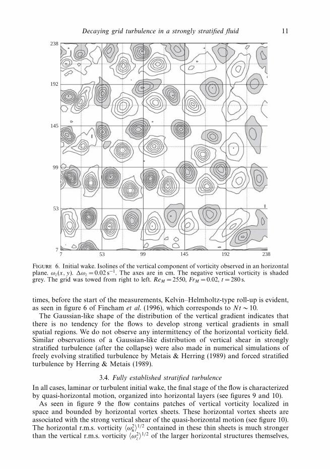
For low U , immediately after the passage of the rake, a regular von Karman type ofvortex shedding is observed in the horizontal plane (see figure 6).
Behind each plate of the rake, we observe the formation of columnar vortex pairs,initially straight and uniform along the vertical. These columnar vortices rapidlyexhibit symmetric sinusoidal deformation as can be seen in figure 7. The shed vorticesdecorrelate vertically, eventually producing multiple layers of eddies. The verticallyuniform flow is thus unstable and no straight columnar vortices persist.
The mechanisms of layer formation and the selection of their vertical scale isstill not clearly understood. Spontaneous generation of layers by a so-called zig-zaginstability is proposed by Billant & Chomaz (2000b). A vertical columnar vortex paircreated by a long pair of vertical flaps is sliced into layers of ‘pancake’ dipole bythis instability. The vertical scale selected by this mechanism is the most amplifiedwavelength of the instability and is proportional to U/N , the buoyancy length scale.Flow decorrelation and layering of eddies can also be induced by a weak, verticallydependent, horizontal velocity as discussed by Majda & Grote (1997). The vertical
10 O. Praud, A. M. Fincham and J. Sommeria
10 100
10–1
10–2
10–3
10–4
10–5
10–6
Ev
Eh
Kin
etic
ene
rgy
(cm
2 s–2
)
Time × U/M
Figure 5. Comparison of the horizontal kinetic energy Eh and the estimated vertical kineticenergy Ev . ReM = 18 000, FrM = 0.17.
scale is then set by the weak external shear. We observed that imperfections in thedensity profile (stronger or weaker stratification) influence the layer positions. Inany case, we shall see in § 3.5 that the vertical scale in the turbulent regime is notinfluenced by this initial behaviour.
3.3. Turbulent initial wake
For higher towing speeds, i.e higher Reynolds numbers, ReM =O(104), and higherFroude numbers, the flow immediately behind the rake is highly three-dimensional, asshown by direct observation. This active turbulence rapidly collapses, after Nt ∼ 30,under the effect of stratification as the vertical velocity component is suppressed. Itresults in multiple layers of quasi-horizontal vortical structures.
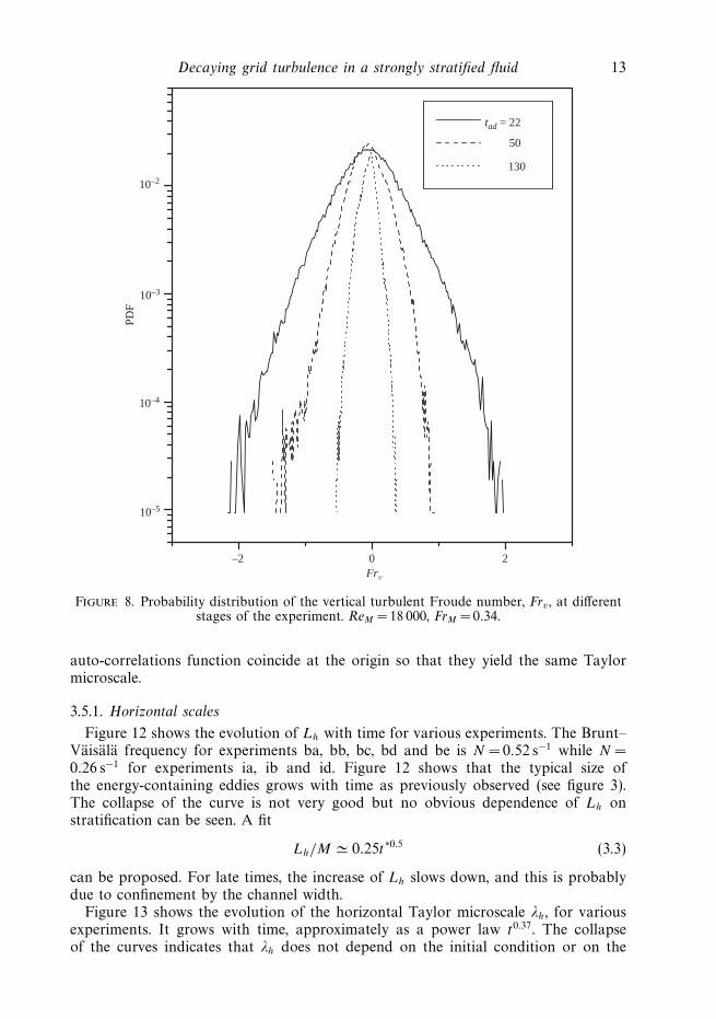
The structures that emerge after the collapse of three-dimensional turbulence aresuch that the gradient Richardson number, Ri = N 2/(∂ux/∂z)2, is found to be greaterthan the critical value for stability: Ric = 1/4. So no overturning instability is expectedand the fluid remains stable with respect to the vertical shear as the Richardsonnumber continues to increase with time. Figure 8 shows the probability distributionfunction of the vertical turbulent Froude number Frv = (∂ux/∂z)/N for different times.The vertical Froude number is directly related to the Richardson number by Fr−2
v = Riso the critical Richardson number correspond to a critical value of Frv equal to 2.It appears that by the time of our first measurement Frv does not exceed the criticalvalue, so the vertical shear is not strong enough to produce overturning. At early
Decaying grid turbulence in a strongly stratified fluid 11
238
192
99
53
77 53 99 145 192 238
145
Figure 6. Initial wake. Isolines of the vertical component of vorticity observed in an horizontalplane. ωz(x, y). ωz =0.02 s−1. The axes are in cm. The negative vertical vorticity is shadedgrey. The grid was towed from right to left. ReM = 2550, FrM = 0.02, t = 280 s.
times, before the start of the measurements, Kelvin–Helmholtz-type roll-up is evident,as seen in figure 6 of Fincham et al. (1996), which corresponds to Nt ∼ 10.
The Gaussian-like shape of the distribution of the vertical gradient indicates thatthere is no tendency for the flows to develop strong vertical gradients in smallspatial regions. We do not observe any intermittency of the horizontal vorticity field.Similar observations of a Gaussian-like distribution of vertical shear in stronglystratified turbulence (after the collapse) were also made in numerical simulations offreely evolving stratified turbulence by Metais & Herring (1989) and forced stratifiedturbulence by Herring & Metais (1989).
3.4. Fully established stratified turbulence
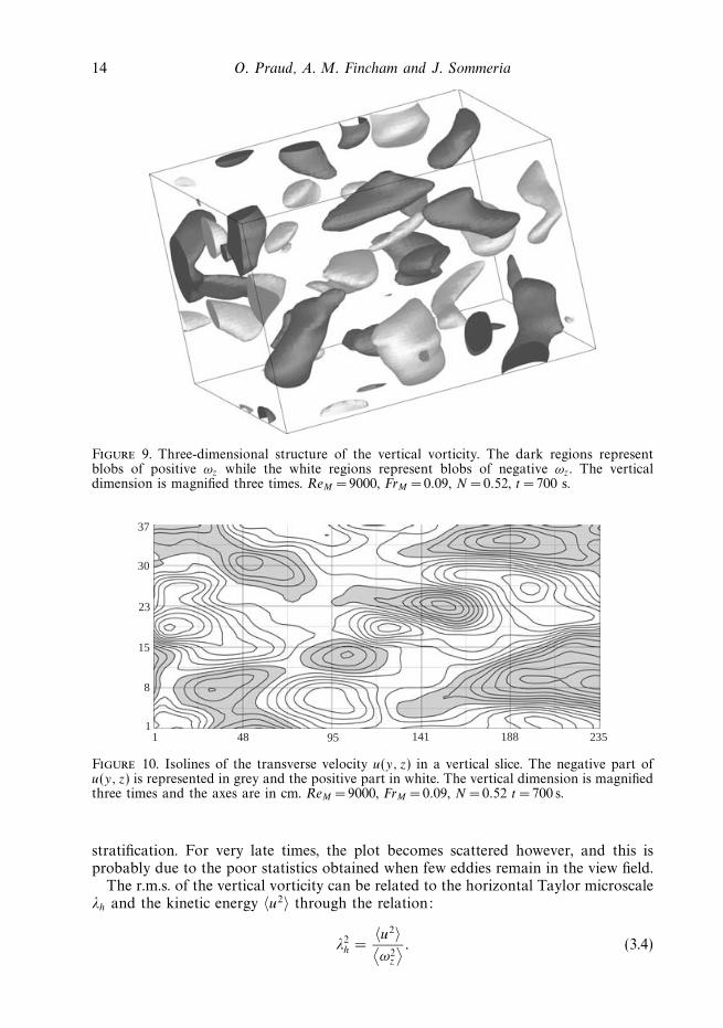
In all cases, laminar or turbulent initial wake, the final stage of the flow is characterizedby quasi-horizontal motion, organized into horizontal layers (see figures 9 and 10).
As seen in figure 9 the flow contains patches of vertical vorticity localized inspace and bounded by horizontal vortex sheets. These horizontal vortex sheets areassociated with the strong vertical shear of the quasi-horizontal motion (see figure 10).The horizontal r.m.s. vorticity 〈ω2
h〉1/2 contained in these thin sheets is much strongerthan the vertical r.m.s. vorticity 〈ω2
z〉1/2 of the larger horizontal structures themselves,
12 O. Praud, A. M. Fincham and J. Sommeria
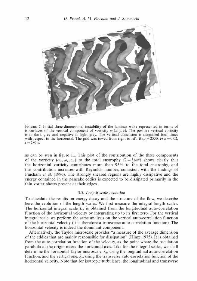
Figure 7. Initial three-dimensional instability of the laminar wake represented in terms ofisosurfaces of the vertical component of vorticity ωz(x, y, z). The positive vertical vorticityis in dark grey and negative in light grey. The vertical dimension is magnified four timeswith respect to the horizontal. The grid was towed from right to left. ReM = 2550, FrM = 0.02,t = 280 s.
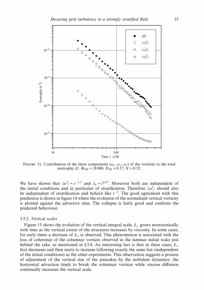
as can be seen in figure 11. This plot of the contribution of the three componentsof the vorticity (ωx, ωy, ωz) to the total enstrophy Ω = 1
2〈ω2〉 shows clearly that
the horizontal vorticity contributes more than 95% to the total enstrophy, andthis contribution increases with Reynolds number, consistent with the findings ofFincham et al. (1996). The strongly sheared regions are highly dissipative and theenergy contained in the pancake eddies is expected to be dissipated primarily in thethin vortex sheets present at their edges.
3.5. Length scale evolution
To elucidate the results on energy decay and the structure of the flow, we describehere the evolution of the length scales. We first measure the integral length scales.The horizontal integral scale Lh is obtained from the longitudinal auto-correlationfunction of the horizontal velocity by integrating up to its first zero. For the verticalintegral scale, we perform the same analysis on the vertical auto-correlation functionof the horizontal velocity (it is therefore a transverse auto-correlation function). Thehorizontal velocity is indeed the dominant component.
Alternatively, the Taylor microscale provides “a measure of the average dimensionof the eddies that are mainly responsible for dissipation” (Hinze 1975). It is obtainedfrom the auto-correlation function of the velocity, as the point where the osculationparabola at the origin meets the horizontal axis. Like for the integral scales, we shalldetermine the horizontal Taylor microscale, λh, using the longitudinal auto-correlationfunction, and the vertical one, λv , using the transverse auto-correlation function of thehorizontal velocity. Note that for isotropic turbulence, the longitudinal and transverse
Decaying grid turbulence in a strongly stratified fluid 13
–2 0 2
10–2
10–3
10–4
10–5
Frv
tad = 22
50
130
PD
F
Figure 8. Probability distribution of the vertical turbulent Froude number, Frv , at differentstages of the experiment. ReM = 18 000, FrM = 0.34.
auto-correlations function coincide at the origin so that they yield the same Taylormicroscale.
3.5.1. Horizontal scales
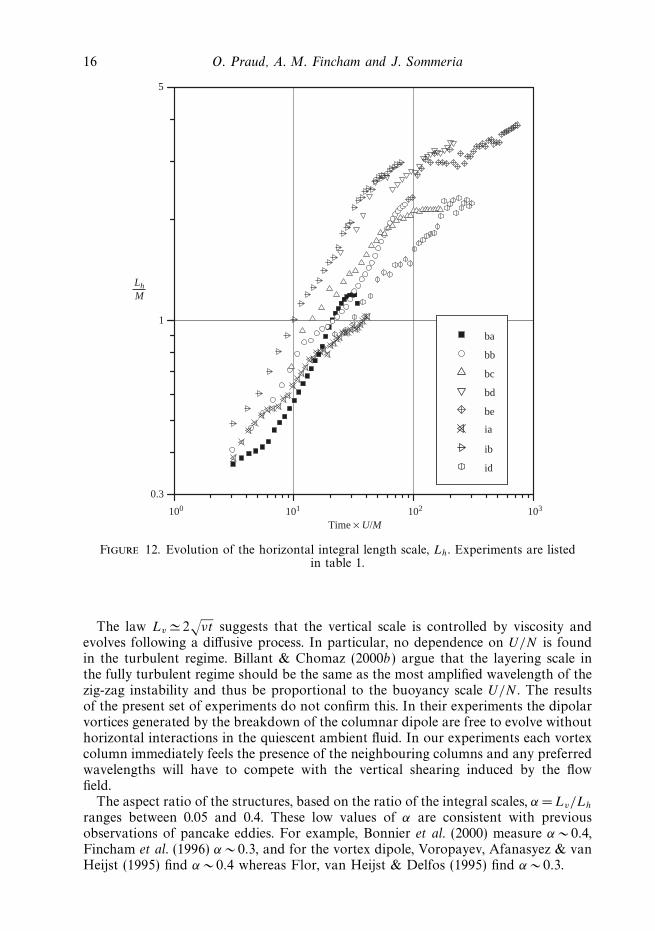
Figure 12 shows the evolution of Lh with time for various experiments. The Brunt–Vaisala frequency for experiments ba, bb, bc, bd and be is N = 0.52 s−1 while N =0.26 s−1 for experiments ia, ib and id. Figure 12 shows that the typical size ofthe energy-containing eddies grows with time as previously observed (see figure 3).The collapse of the curve is not very good but no obvious dependence of Lh onstratification can be seen. A fit
Lh/M 0.25t∗0.5 (3.3)
can be proposed. For late times, the increase of Lh slows down, and this is probablydue to confinement by the channel width.
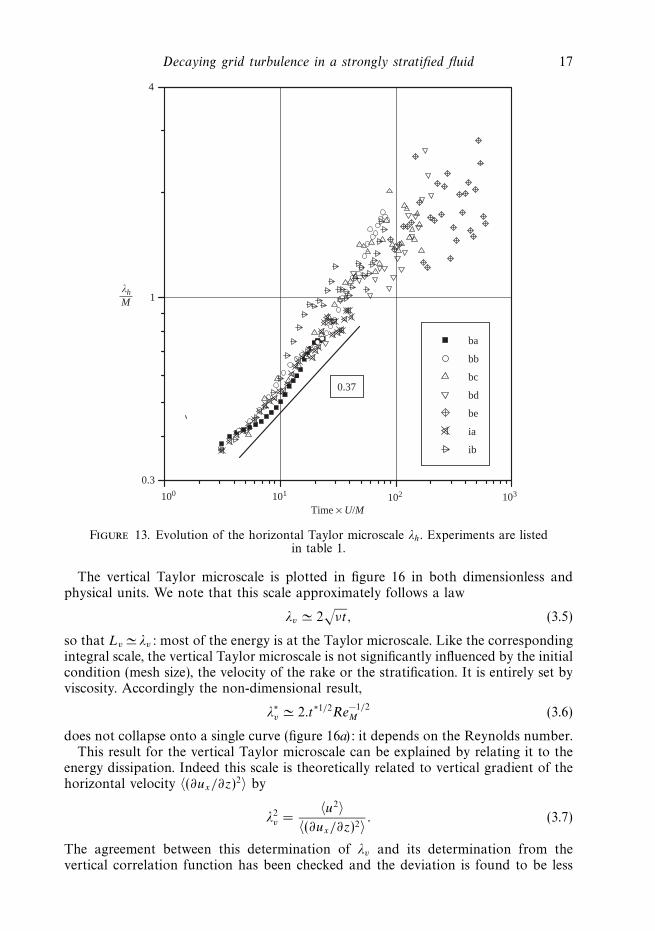
Figure 13 shows the evolution of the horizontal Taylor microscale λh, for variousexperiments. It grows with time, approximately as a power law t0.37. The collapseof the curves indicates that λh does not depend on the initial condition or on the
14 O. Praud, A. M. Fincham and J. Sommeria
Figure 9. Three-dimensional structure of the vertical vorticity. The dark regions representblobs of positive ωz while the white regions represent blobs of negative ωz. The verticaldimension is magnified three times. ReM = 9000, FrM = 0.09, N = 0.52, t = 700 s.
37
30
23
15
8
11 188 2351419548
Figure 10. Isolines of the transverse velocity u(y, z) in a vertical slice. The negative part ofu(y, z) is represented in grey and the positive part in white. The vertical dimension is magnifiedthree times and the axes are in cm. ReM = 9000, FrM = 0.09, N =0.52 t = 700 s.
stratification. For very late times, the plot becomes scattered however, and this isprobably due to the poor statistics obtained when few eddies remain in the view field.
The r.m.s. of the vertical vorticity can be related to the horizontal Taylor microscaleλh and the kinetic energy 〈u2〉 through the relation:
λ2h =
〈u2〉⟨ω2
z
⟩ . (3.4)
Decaying grid turbulence in a strongly stratified fluid 15
10 100
10–2
10–3
10–4
10–5
2Ω
ωx2
ωy2
ωy2
Ens
trop
hy (
s–2)
Time × U/M
Figure 11. Contribution of the three components (ωx, ωy, ωz) of the vorticity to the totalenstrophy Ω . ReM =18 000, FrM =0.17, N = 0.52.
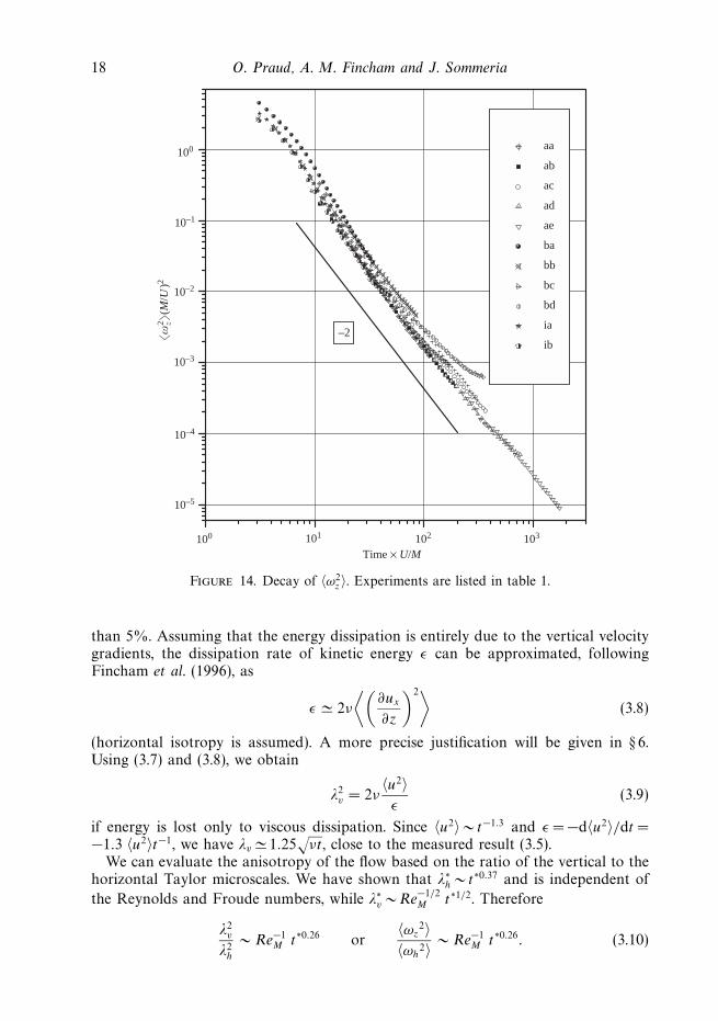
We have shown that 〈u2〉 ∼ t−1.3 and λh ∼ t0.37. Moreover both are independent ofthe initial conditions and in particular of stratification. Therefore 〈ω2
z〉 should alsobe independent of stratification and behave like t−2. The good agreement with thisprediction is shown in figure 14 where the evolution of the normalized vertical vorticityis plotted against the advective time. The collapse is fairly good and confirms thepredicted behaviour.
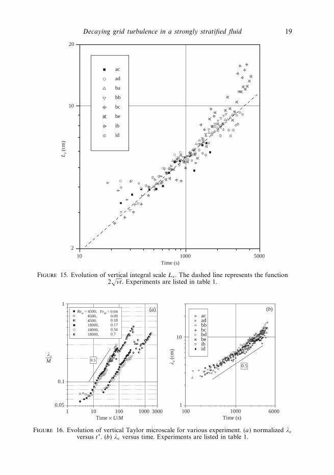
3.5.2. Vertical scales
Figure 15 shows the evolution of the vertical integral scale. Lv grows monotonicallywith time as the vertical extent of the structures increases by viscosity. In some cases,for early times a decrease of Lv is observed. This phenomenon is associated with theloss of coherence of the columnar vortices observed in the laminar initial wake justbehind the rake, as mentioned in § 3.4. An interesting fact is that in these cases, Lv
first decreases and then starts to increase following exactly the same law (independentof the initial conditions) as the other experiments. This observation suggests a processof adjustment of the vertical size of the pancakes by the turbulent dynamics: thehorizontal advection tends to break the columnar vortices while viscous diffusioncontinually increases the vertical scale.
16 O. Praud, A. M. Fincham and J. Sommeria
100 101 102 103
0.3
1
5
Lh
Time × U/M
ba
bb
bc
bd
be
ib
ia
id
M
Figure 12. Evolution of the horizontal integral length scale, Lh. Experiments are listedin table 1.
The law Lv 2√
νt suggests that the vertical scale is controlled by viscosity andevolves following a diffusive process. In particular, no dependence on U/N is foundin the turbulent regime. Billant & Chomaz (2000b) argue that the layering scale inthe fully turbulent regime should be the same as the most amplified wavelength of thezig-zag instability and thus be proportional to the buoyancy scale U/N . The resultsof the present set of experiments do not confirm this. In their experiments the dipolarvortices generated by the breakdown of the columnar dipole are free to evolve withouthorizontal interactions in the quiescent ambient fluid. In our experiments each vortexcolumn immediately feels the presence of the neighbouring columns and any preferredwavelengths will have to compete with the vertical shearing induced by the flowfield.
The aspect ratio of the structures, based on the ratio of the integral scales, α = Lv/Lh
ranges between 0.05 and 0.4. These low values of α are consistent with previousobservations of pancake eddies. For example, Bonnier et al. (2000) measure α ∼ 0.4,Fincham et al. (1996) α ∼ 0.3, and for the vortex dipole, Voropayev, Afanasyez & vanHeijst (1995) find α ∼ 0.4 whereas Flor, van Heijst & Delfos (1995) find α ∼ 0.3.
Decaying grid turbulence in a strongly stratified fluid 17
100 101 102 103
0.3
1
4
0.37
λh
Time × U/M
ba
bb
bc
bd
be
ia
ib
M
Figure 13. Evolution of the horizontal Taylor microscale λh. Experiments are listedin table 1.
The vertical Taylor microscale is plotted in figure 16 in both dimensionless andphysical units. We note that this scale approximately follows a law
λv 2√
νt, (3.5)
so that Lv λv: most of the energy is at the Taylor microscale. Like the correspondingintegral scale, the vertical Taylor microscale is not significantly influenced by the initialcondition (mesh size), the velocity of the rake or the stratification. It is entirely set byviscosity. Accordingly the non-dimensional result,
λ∗v 2.t∗1/2Re−1/2
M (3.6)
does not collapse onto a single curve (figure 16a): it depends on the Reynolds number.This result for the vertical Taylor microscale can be explained by relating it to the
energy dissipation. Indeed this scale is theoretically related to vertical gradient of thehorizontal velocity 〈(∂ux/∂z)2〉 by
λ2v =
〈u2〉〈(∂ux/∂z)2〉 . (3.7)
The agreement between this determination of λv and its determination from thevertical correlation function has been checked and the deviation is found to be less
18 O. Praud, A. M. Fincham and J. Sommeria
100
10–1
10–2
10–3
10–4
10–5
100 101 102 103
–2
aa
ab
ac
ad
ae
ba
bb
bc
bd
ia
ib
ωz2
(M/U
)2
Time × U/M
Figure 14. Decay of 〈ω2z〉. Experiments are listed in table 1.
than 5%. Assuming that the energy dissipation is entirely due to the vertical velocitygradients, the dissipation rate of kinetic energy ε can be approximated, followingFincham et al. (1996), as
ε 2ν
⟨(∂ux
∂z
)2⟩(3.8)
(horizontal isotropy is assumed). A more precise justification will be given in § 6.Using (3.7) and (3.8), we obtain
λ2v = 2ν
〈u2〉ε
(3.9)
if energy is lost only to viscous dissipation. Since 〈u2〉 ∼ t−1.3 and ε = −d〈u2〉/dt =−1.3 〈u2〉t−1, we have λv 1.25
√νt , close to the measured result (3.5).
We can evaluate the anisotropy of the flow based on the ratio of the vertical to thehorizontal Taylor microscales. We have shown that λ∗
h ∼ t∗0.37 and is independent of
the Reynolds and Froude numbers, while λ∗v ∼ Re−1/2
M t∗1/2. Therefore
λ2v
λ2h
∼ Re−1M t∗0.26 or
〈ωz2〉
〈ωh2〉 ∼ Re−1
M t∗0.26. (3.10)
Decaying grid turbulence in a strongly stratified fluid 19
10 1000 5000
2
10
20
ac
ad
ba
bb
bc
be
ib
id
Lv
(cm
)
Time (s)
Figure 15. Evolution of vertical integral scale Lv . The dashed line represents the function2
√νt . Experiments are listed in table 1.
1 10 100 1000 30000.05
0.1
1
0.5
(a)
λv
Time × U/M
Rem = 4500,
100 1000 60001
10
(b)acadbbbcbdbeibid
0.5λv
(cm
)
Time (s)
FrM = 0.044500,4500,18000,
18000,18000,
0.090.180.170.340.7
M
Figure 16. Evolution of vertical Taylor microscale for various experiment. (a) normalized λv
versus t∗. (b) λv versus time. Experiments are listed in table 1.
20 O. Praud, A. M. Fincham and J. Sommeria
10–2 10–1
100
10–1
10–2
10–3
10–4
t* = 3
8
15
27
37
50
66
84
–2.0
–3.8
E(kh)
kh
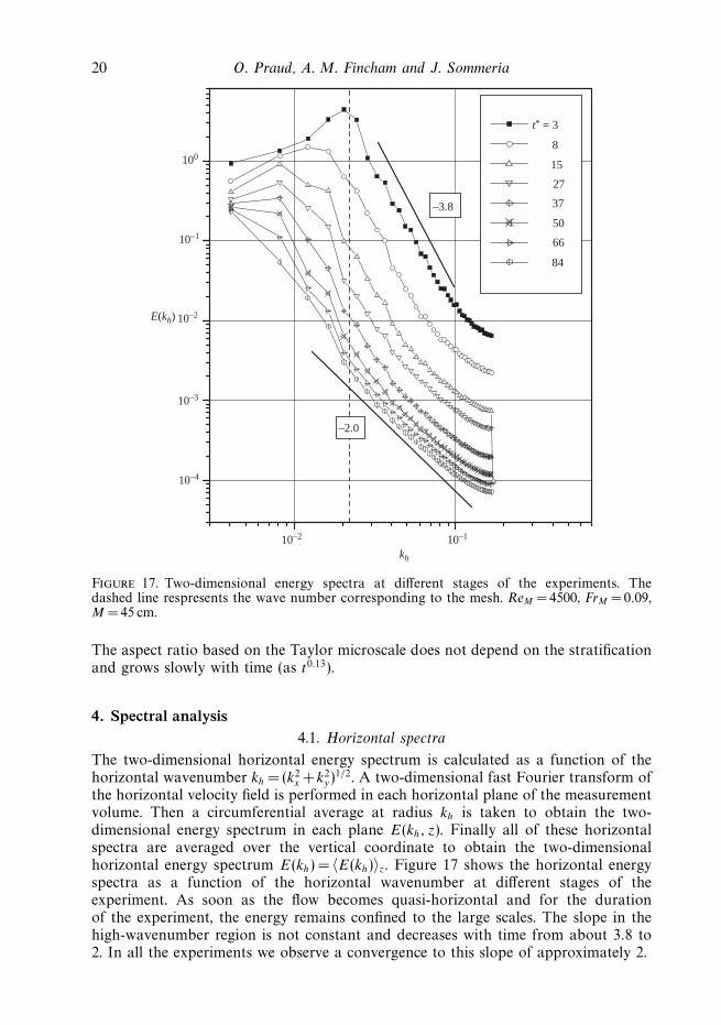
Figure 17. Two-dimensional energy spectra at different stages of the experiments. Thedashed line respresents the wave number corresponding to the mesh. ReM = 4500, FrM = 0.09,M =45 cm.
The aspect ratio based on the Taylor microscale does not depend on the stratificationand grows slowly with time (as t0.13).
4. Spectral analysis4.1. Horizontal spectra
The two-dimensional horizontal energy spectrum is calculated as a function of thehorizontal wavenumber kh = (k2
x +k2y)
1/2. A two-dimensional fast Fourier transform ofthe horizontal velocity field is performed in each horizontal plane of the measurementvolume. Then a circumferential average at radius kh is taken to obtain the two-dimensional energy spectrum in each plane E(kh, z). Finally all of these horizontalspectra are averaged over the vertical coordinate to obtain the two-dimensionalhorizontal energy spectrum E(kh) = 〈E(kh)〉z. Figure 17 shows the horizontal energyspectra as a function of the horizontal wavenumber at different stages of theexperiment. As soon as the flow becomes quasi-horizontal and for the durationof the experiment, the energy remains confined to the large scales. The slope in thehigh-wavenumber region is not constant and decreases with time from about 3.8 to2. In all the experiments we observe a convergence to this slope of approximately 2.
Decaying grid turbulence in a strongly stratified fluid 21
101
100
10–1
10–2
10–3
10–4
10–2 10–1
ReM = 2250 FrM = 0.02
2250 0.04
4500 0.04
4500 0.09
18000 0.17
18000 0.34
E(kh)
kh
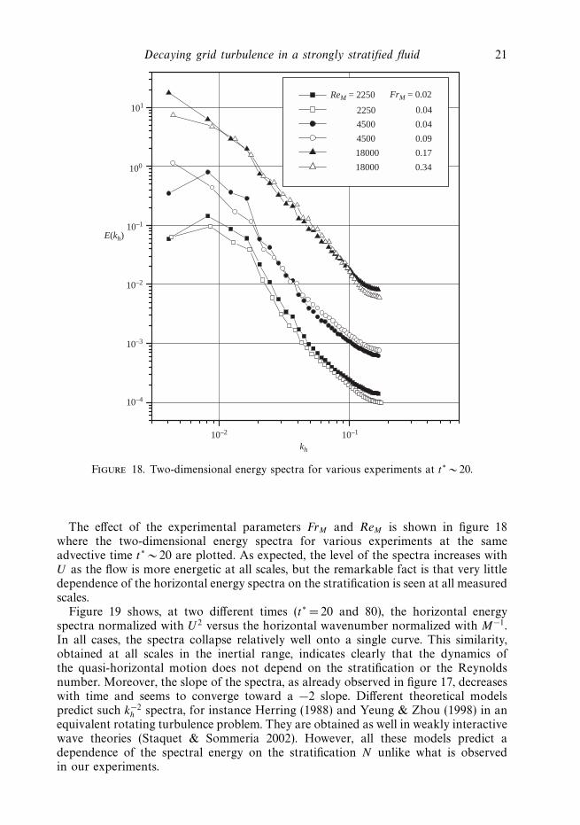
Figure 18. Two-dimensional energy spectra for various experiments at t∗ ∼ 20.
The effect of the experimental parameters FrM and ReM is shown in figure 18where the two-dimensional energy spectra for various experiments at the sameadvective time t∗ ∼ 20 are plotted. As expected, the level of the spectra increases withU as the flow is more energetic at all scales, but the remarkable fact is that very littledependence of the horizontal energy spectra on the stratification is seen at all measuredscales.
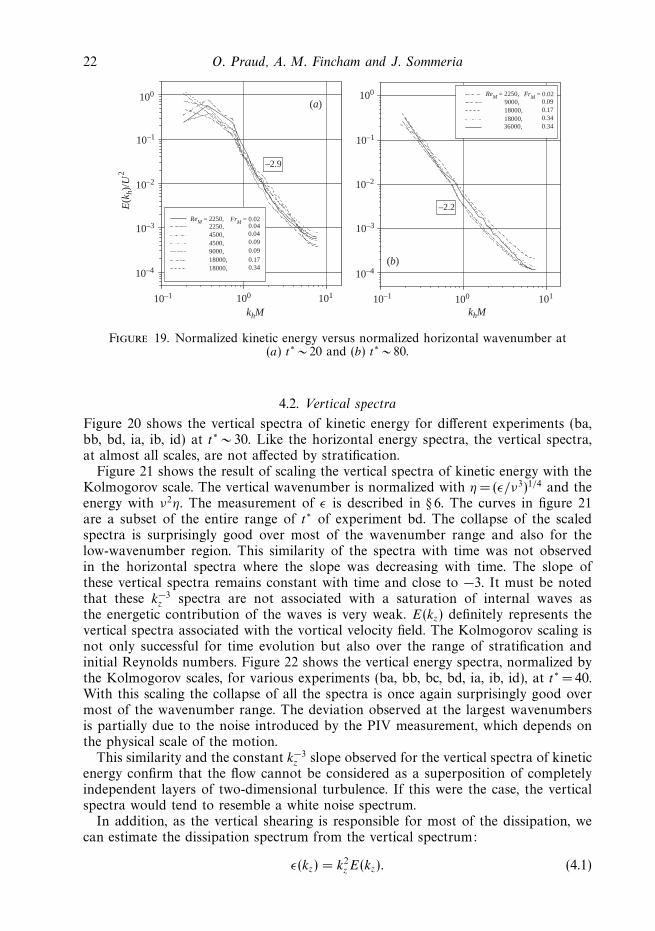
Figure 19 shows, at two different times (t∗ = 20 and 80), the horizontal energyspectra normalized with U 2 versus the horizontal wavenumber normalized with M−1.In all cases, the spectra collapse relatively well onto a single curve. This similarity,obtained at all scales in the inertial range, indicates clearly that the dynamics ofthe quasi-horizontal motion does not depend on the stratification or the Reynoldsnumber. Moreover, the slope of the spectra, as already observed in figure 17, decreaseswith time and seems to converge toward a −2 slope. Different theoretical modelspredict such k−2
h spectra, for instance Herring (1988) and Yeung & Zhou (1998) in anequivalent rotating turbulence problem. They are obtained as well in weakly interactivewave theories (Staquet & Sommeria 2002). However, all these models predict adependence of the spectral energy on the stratification N unlike what is observedin our experiments.
22 O. Praud, A. M. Fincham and J. Sommeria
10110010–1
100
10–1
10–2
10–3
10–4
–2.9
ReM = 2250,
E(k
h)/U
2
khM
100
10–1
10–2
10–3
10–4
10–1 100 101
–2.2
khM
FrM = 0.02
ReM = 2250, FrM = 0.02
2250, 0.04
9000,18000,18000,36000,
0.090.170.340.34
0.040.090.09
0.170.34
4500,4500,9000,18000,18000,
(a)
(b)
Figure 19. Normalized kinetic energy versus normalized horizontal wavenumber at(a) t∗ ∼ 20 and (b) t∗ ∼ 80.
4.2. Vertical spectra
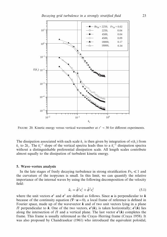
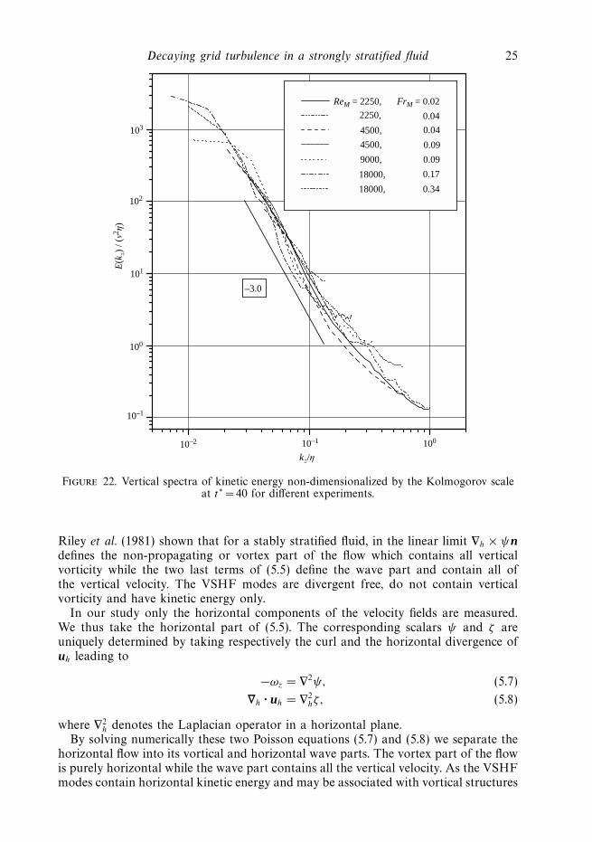
Figure 20 shows the vertical spectra of kinetic energy for different experiments (ba,bb, bd, ia, ib, id) at t∗ ∼ 30. Like the horizontal energy spectra, the vertical spectra,at almost all scales, are not affected by stratification.
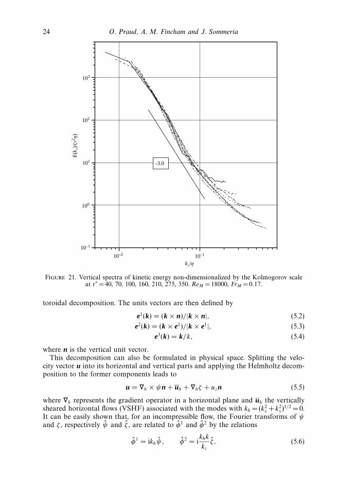
Figure 21 shows the result of scaling the vertical spectra of kinetic energy with theKolmogorov scale. The vertical wavenumber is normalized with η = (ε/ν3)1/4 and theenergy with ν2η. The measurement of ε is described in § 6. The curves in figure 21are a subset of the entire range of t∗ of experiment bd. The collapse of the scaledspectra is surprisingly good over most of the wavenumber range and also for thelow-wavenumber region. This similarity of the spectra with time was not observedin the horizontal spectra where the slope was decreasing with time. The slope ofthese vertical spectra remains constant with time and close to −3. It must be notedthat these k−3
z spectra are not associated with a saturation of internal waves asthe energetic contribution of the waves is very weak. E(kz) definitely represents thevertical spectra associated with the vortical velocity field. The Kolmogorov scaling isnot only successful for time evolution but also over the range of stratification andinitial Reynolds numbers. Figure 22 shows the vertical energy spectra, normalized bythe Kolmogorov scales, for various experiments (ba, bb, bc, bd, ia, ib, id), at t∗ = 40.With this scaling the collapse of all the spectra is once again surprisingly good overmost of the wavenumber range. The deviation observed at the largest wavenumbersis partially due to the noise introduced by the PIV measurement, which depends onthe physical scale of the motion.
This similarity and the constant k−3z slope observed for the vertical spectra of kinetic
energy confirm that the flow cannot be considered as a superposition of completelyindependent layers of two-dimensional turbulence. If this were the case, the verticalspectra would tend to resemble a white noise spectrum.
In addition, as the vertical shearing is responsible for most of the dissipation, wecan estimate the dissipation spectrum from the vertical spectrum:
ε(kz) = k2zE(kz). (4.1)
Decaying grid turbulence in a strongly stratified fluid 23
101
100
10–1
10–2
10–3
10–4
10–5
10–2 10–1 100
ReM = 2250, FrM = 0.02
2250, 0.04
4500, 0.04
4500, 0.09
18000, 0.1718000, 0.34
E(kz)
kz
Figure 20. Kinetic energy versus vertical wavenumber at t∗ ∼ 30 for different experiments.
The dissipation associated with each scale kz is then given by integration of ε(kz) fromkz to 2kz. The k−3
z slope of the vertical spectra leads thus to a k−1z dissipation spectra
without a distinguishable preferential dissipation scale. All length scales contributealmost equally to the dissipation of turbulent kinetic energy.
5. Wave–vortex analysisIn the late stages of freely decaying turbulence in strong stratification Frh 1 and
the curvature of the isopycnes is small. In this limit, we can quantify the relativeimportance of the internal waves by using the following decomposition of the velocityfield:
ui = φ1e1i + φ2e2
i (5.1)
where the unit vectors e1 and e2 are defined as follows. Since u is perpendicular to kbecause of the continuity equation (∇ · u =0), a local frame of reference is defined inFourier space, made up of the wavevector k and of two unit vectors lying in a planeΠ perpendicular to k. One of the two vectors, e1(k), is taken horizontally; e2(k) liesalong the intersection of Π and a vertical plane. The last vector e3(k) completes theframe. This frame is usually referenced as the Craya–Herring frame (Craya 1958). Itwas also proposed by Chandrasekar (1961) who introduced the equivalent poloidal,
24 O. Praud, A. M. Fincham and J. Sommeria
103
102
101
100
10–1
10–2 10–1
–3.0
E(k
z)/(ν2 η
)
kz/η
Figure 21. Vertical spectra of kinetic energy non-dimensionalized by the Kolmogorov scaleat t∗ = 40, 70, 100, 160, 210, 275, 350. ReM = 18000, FrM = 0.17.
toroidal decomposition. The units vectors are then defined by
e1(k) = (k × n)/|k × n|, (5.2)
e2(k) = (k × e1)/|k × e1|, (5.3)
e3(k) = k/k, (5.4)
where n is the vertical unit vector.This decomposition can also be formulated in physical space. Splitting the velo-
city vector u into its horizontal and vertical parts and applying the Helmholtz decom-position to the former components leads to
u = ∇h × ψn + uh + ∇hζ + uzn (5.5)
where ∇h represents the gradient operator in a horizontal plane and uh the verticallysheared horizontal flows (VSHF) associated with the modes with kh = (k2
x + k2y)
1/2 = 0.It can be easily shown that, for an incompressible flow, the Fourier transforms of ψ
and ζ , respectively ψ and ζ , are related to φ1 and φ2 by the relations
φ1 = ikhψ, φ2 = ikhk
kz
ζ . (5.6)
Decaying grid turbulence in a strongly stratified fluid 25
103
102
101
100
10–1
10–2 10–1 100
–3.0
ReM = 2250, FrM = 0.02
2250, 0.04
4500, 0.04
4500, 0.09
9000, 0.09
18000, 0.17
18000, 0.34
E(k
z) /
(ν2 η
)
kz/η
Figure 22. Vertical spectra of kinetic energy non-dimensionalized by the Kolmogorov scaleat t∗ =40 for different experiments.
Riley et al. (1981) shown that for a stably stratified fluid, in the linear limit ∇h × ψndefines the non-propagating or vortex part of the flow which contains all verticalvorticity while the two last terms of (5.5) define the wave part and contain all ofthe vertical velocity. The VSHF modes are divergent free, do not contain verticalvorticity and have kinetic energy only.
In our study only the horizontal components of the velocity fields are measured.We thus take the horizontal part of (5.5). The corresponding scalars ψ and ζ areuniquely determined by taking respectively the curl and the horizontal divergence ofuh leading to
−ωz = ∇2ψ, (5.7)
∇h · uh = ∇2hζ, (5.8)
where ∇2h denotes the Laplacian operator in a horizontal plane.
By solving numerically these two Poisson equations (5.7) and (5.8) we separate thehorizontal flow into its vortical and horizontal wave parts. The vortex part of the flowis purely horizontal while the wave part contains all the vertical velocity. As the VSHFmodes contain horizontal kinetic energy and may be associated with vortical structures
26 O. Praud, A. M. Fincham and J. Sommeria
10–1
10–2
10–3
10–4
10–5
10–6
102 103
Kin
etic
ene
rgy
(cm
2 s–2
)
Time × U/M
Figure 23. Evolution of the total kinetic energy (black squares), vortex horizontal kineticenergy (circles), wave kinetic energy (upward triangles) and vertical kinetic energy (downwardtriangles). ReM = 9000, FrM = 0.08, N = 0.52.
much larger than the measurement area, they are included in the vortical part of ourdecomposition.
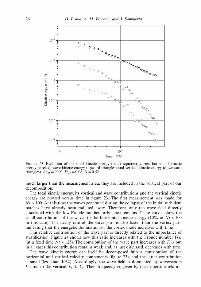
The total kinetic energy, its vortical and wave contributions and the vertical kineticenergy are plotted versus time in figure 23. The first measurement was made forNt ∼ 100. At this time the waves generated during the collapse of the initial turbulentpatches have already been radiated away. Therefore, only the wave field directlyassociated with the low-Froude-number turbulence remains. These curves show thesmall contribution of the waves to the horizontal kinetic energy (10% at Nt ∼ 100in this case). The decay rate of the wave part is also faster than the vortex part,indicating that the energetic domination of the vortex mode increases with time.
This relative contribution of the wave part is directly related to the importance ofstratification. Figure 24 shows how this ratio increases with the Froude number FrM
(at a fixed time Nt ∼ 125). The contribution of the wave part increases with FrM butin all cases this contribution remains weak and, as just discussed, decreases with time.
The wave kinetic energy can itself be decomposed into a contribution of thehorizontal and vertical velocity components (figure 23), and the latter contributionis small (less than 10%). Accordingly, the wave field is dominated by wavevectorsk close to the vertical, kz kh. Their frequency ω, given by the dispersion relation
Decaying grid turbulence in a strongly stratified fluid 27
0 0.1 0.2 0.3
0.1
0.2
EW
FrM
EV
Figure 24. Ratio of the horizontal kinetic energy of the wave part to the total horizontalkinetic energy versus Froude number. Nt ∼ 125. Experiments aa, ab, ac, ba, bc, bd, ia, ib.
ω2 = N 2k2h(k
2h + k2
z)−1, is therefore much smaller than N . We can estimate that this
is close to the advective frequency u/Lh =N/Fr N , allowing strong interactionsbetween the vortical and wave modes.
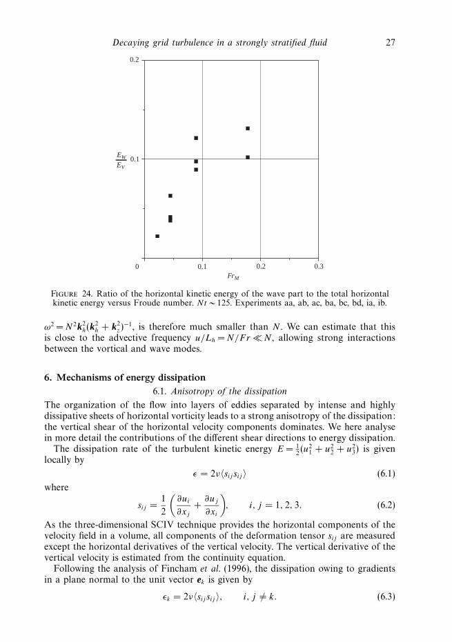
6. Mechanisms of energy dissipation6.1. Anisotropy of the dissipation
The organization of the flow into layers of eddies separated by intense and highlydissipative sheets of horizontal vorticity leads to a strong anisotropy of the dissipation:the vertical shear of the horizontal velocity components dominates. We here analysein more detail the contributions of the different shear directions to energy dissipation.
The dissipation rate of the turbulent kinetic energy E = 12(u2
1 + u22 + u2
3) is givenlocally by
ε = 2ν〈sij sij 〉 (6.1)
where
sij =1
2
(∂ui
∂xj
+∂uj
∂xi
), i, j = 1, 2, 3. (6.2)
As the three-dimensional SCIV technique provides the horizontal components of thevelocity field in a volume, all components of the deformation tensor sij are measuredexcept the horizontal derivatives of the vertical velocity. The vertical derivative of thevertical velocity is estimated from the continuity equation.
Following the analysis of Fincham et al. (1996), the dissipation owing to gradientsin a plane normal to the unit vector ek is given by
εk = 2ν〈sij sij 〉, i, j = k. (6.3)
28 O. Praud, A. M. Fincham and J. Sommeria
10–3
10–4
10–5
10–6
10–7
101 102
Dis
sipa
tion
rat
e (c
m2
s–3)
Time × U/M
ε
εx
εy
εz
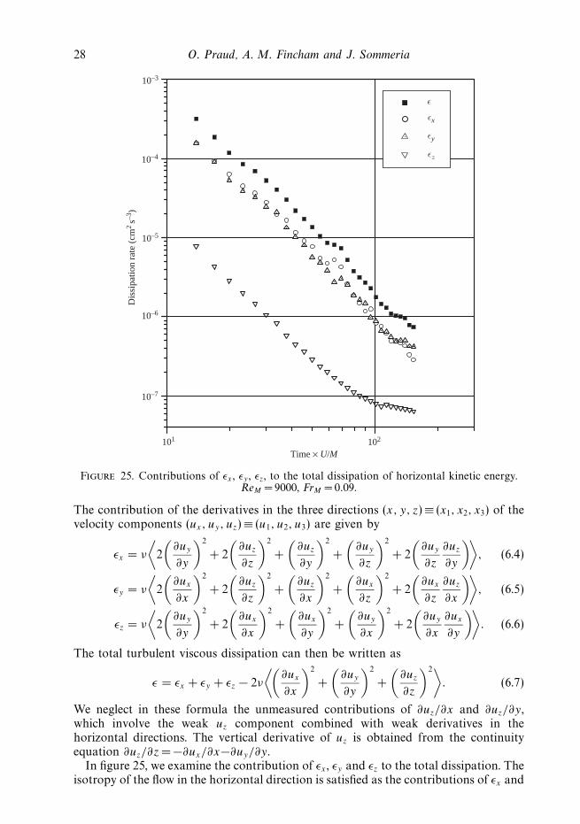
Figure 25. Contributions of εx , εy , εz, to the total dissipation of horizontal kinetic energy.ReM = 9000, FrM = 0.09.
The contribution of the derivatives in the three directions (x, y, z) ≡ (x1, x2, x3) of thevelocity components (ux, uy, uz) ≡ (u1, u2, u3) are given by
εx = ν
⟨2
(∂uy
∂y
)2
+ 2
(∂uz
∂z
)2
+
(∂uz
∂y
)2
+
(∂uy
∂z
)2
+ 2
(∂uy
∂z
∂uz
∂y
)⟩, (6.4)
εy = ν
⟨2
(∂ux
∂x
)2
+ 2
(∂uz
∂z
)2
+
(∂uz
∂x
)2
+
(∂ux
∂z
)2
+ 2
(∂ux
∂z
∂uz
∂x
)⟩, (6.5)
εz = ν
⟨2
(∂uy
∂y
)2
+ 2
(∂ux
∂x
)2
+
(∂ux
∂y
)2
+
(∂uy
∂x
)2
+ 2
(∂uy
∂x
∂ux
∂y
)⟩. (6.6)
The total turbulent viscous dissipation can then be written as
ε = εx + εy + εz − 2ν
⟨(∂ux
∂x
)2
+
(∂uy
∂y
)2
+
(∂uz
∂z
)2⟩. (6.7)
We neglect in these formula the unmeasured contributions of ∂uz/∂x and ∂uz/∂y,which involve the weak uz component combined with weak derivatives in thehorizontal directions. The vertical derivative of uz is obtained from the continuityequation ∂uz/∂z = −∂ux/∂x−∂uy/∂y.
In figure 25, we examine the contribution of εx , εy and εz to the total dissipation. Theisotropy of the flow in the horizontal direction is satisfied as the contributions of εx and
Decaying grid turbulence in a strongly stratified fluid 29
10–4
10–5
10–6
102 103
Dis
sipa
tion
rat
e (c
m2
s–3)
Time (s)
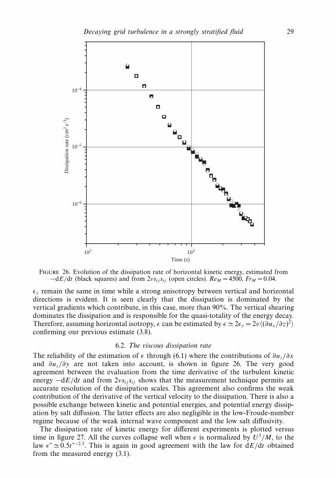
Figure 26. Evolution of the dissipation rate of horizontal kinetic energy, estimated from−dE/dt (black squares) and from 2νsij sij (open circles). ReM = 4500, FrM = 0.04.
εy remain the same in time while a strong anisotropy between vertical and horizontaldirections is evident. It is seen clearly that the dissipation is dominated by thevertical gradients which contribute, in this case, more than 90%. The vertical shearingdominates the dissipation and is responsible for the quasi-totality of the energy decay.Therefore, assuming horizontal isotropy, ε can be estimated by ε 2εy = 2ν〈(∂ux/∂z)2〉confirming our previous estimate (3.8).
6.2. The viscous dissipation rate
The reliability of the estimation of ε through (6.1) where the contributions of ∂uz/∂x
and ∂uz/∂y are not taken into account, is shown in figure 26. The very goodagreement between the evaluation from the time derivative of the turbulent kineticenergy −dE/dt and from 2νsij sij shows that the measurement technique permits anaccurate resolution of the dissipation scales. This agreement also confirms the weakcontribution of the derivative of the vertical velocity to the dissipation. There is also apossible exchange between kinetic and potential energies, and potential energy dissip-ation by salt diffusion. The latter effects are also negligible in the low-Froude-numberregime because of the weak internal wave component and the low salt diffusivity.
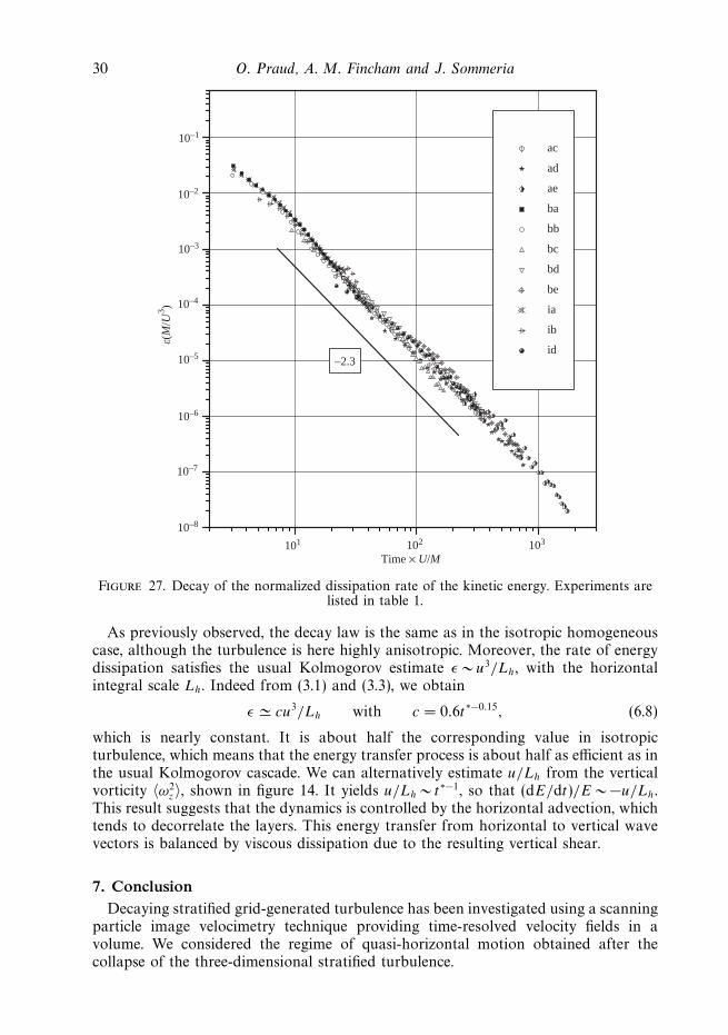
The dissipation rate of kinetic energy for different experiments is plotted versustime in figure 27. All the curves collapse well when ε is normalized by U 3/M , to thelaw ε∗ 0.5t∗−2.3. This is again in good agreement with the law for dE/dt obtainedfrom the measured energy (3.1).
30 O. Praud, A. M. Fincham and J. Sommeria
10–1
10–2
10–3
10–4
10–5
10–6
10–7
10–8
101 102 103
–2.3
ac
ad
ae
ba
bb
bc
bd
be
ia
ib
id
ε(M
/U3 )
Time × U/M
Figure 27. Decay of the normalized dissipation rate of the kinetic energy. Experiments arelisted in table 1.
As previously observed, the decay law is the same as in the isotropic homogeneouscase, although the turbulence is here highly anisotropic. Moreover, the rate of energydissipation satisfies the usual Kolmogorov estimate ε ∼ u3/Lh, with the horizontalintegral scale Lh. Indeed from (3.1) and (3.3), we obtain
ε cu3/Lh with c = 0.6t∗−0.15, (6.8)
which is nearly constant. It is about half the corresponding value in isotropicturbulence, which means that the energy transfer process is about half as efficient as inthe usual Kolmogorov cascade. We can alternatively estimate u/Lh from the verticalvorticity 〈ω2
z〉, shown in figure 14. It yields u/Lh ∼ t∗−1, so that (dE/dt)/E ∼ −u/Lh.This result suggests that the dynamics is controlled by the horizontal advection, whichtends to decorrelate the layers. This energy transfer from horizontal to vertical wavevectors is balanced by viscous dissipation due to the resulting vertical shear.
7. ConclusionDecaying stratified grid-generated turbulence has been investigated using a scanning
particle image velocimetry technique providing time-resolved velocity fields in avolume. We considered the regime of quasi-horizontal motion obtained after thecollapse of the three-dimensional stratified turbulence.
Decaying grid turbulence in a strongly stratified fluid 31
In this regime, we observe the evolution of the flow into a layered field with strongvertical shear. The generation of such horizontal layers shows good agreement withthe results obtained in the numerical simulations of Herring & Metais (1989) or in theexperiments of Fincham et al. (1996). We find the layering scale to be independent ofthe stratification and in particular it does not exhibit any proportionality with U/N .
While the horizontal motion dominates, the vertical shear leads to strong energydissipation and prevents stratified turbulence from exhibiting the characteristics oftwo-dimensional turbulence. This anisotropy of the dissipation process was quantifiedusing a direct measurement of the relative contribution of all the gradients to thedissipation rate. Vertical shearing appears to be responsible for the quasi-totality ofthe energy decay, increasingly so for higher Reynolds numbers.
The present set of experiments demonstrates some important properties of decayingstratified turbulence, once the quasi horizontal motion regime is established. We foundin this regime a self-similar temporal evolution of the energy decay and of the lengthscales. The kinetic energy decay, remarkably, exhibits the same scaling form as three-dimensional isotropic homogeneous turbulence with a scaling exponent close to −1.3,even though the energy dissipation mechanisms are radically different. This valueis also close to the one found in the early stage (before the collapse) of decayingstratified turbulence. The scaling law obtained for the evolution of the vertical scale,Re−0.5
M t∗0.5, is consistent with the model of viscous growth proposed in this paper.Moreover, very little influence of the initial conditions and in particular of the
stratification was observed in either the dynamics or the measured values of the kineticenergy and the horizontal and vertical length scales. Our results can therefore beconsidered as general properties of stratified turbulence independent of the generationmechanism. Furthermore, as pointed out by Riley et al. (1981), whatever the initialFroude number, the turbulence is completely dominated by stratification after a fewBrunt–Vaisala periods. Stratification plays a role in the early stages of the turbulenceevolution by inhibiting the vertical fluxes and provoking its collapse. But, after thecollapse, with the establishment of the quasi-horizontal motion, the dynamics of theflow is no longer controlled by stratification and does not depend on it. In this regime(Fr 1) a self-similarity in the limit of Fr → 0 is suggested by the experiments.
Nevertheless, the dynamics of the turbulence cannot be represented by completelyindependent quasi-horizontal flows. Indeed, we showed that the layers are stronglycoupled by viscosity. A balance between horizontal advection, which tends to verticallydecorrelate the flow, and vertical diffusion is observed. The basic dynamics of energydecay is therefore a transfer from large horizontal to smaller vertical scales, whereviscous dissipation takes place. As a consequence of this viscous coupling, the verticalscales are found to be governed by viscosity and to grow according to a diffusiveprocess that is not influenced by their initial behaviour. Note that all the verticalscales contribute equally to this dissipation because of the k−3
z energy spectrum.Extrapolating these results to very high Reynolds numbers, we find that the vertical
shear scales as ωh ∼ Re0.5. For high Re, the condition for low gradient Richardsonnumber Ri =N 2/ω2
h ∼ N 2Re−1 will clearly be reached, leading to local shear instability.This will lead to the generation of small-scale turbulence that could act as an eddydiffusivity for the larger scales, so our results could apply with a Reynolds numberbased on this eddy diffusivity. In particular the scaling laws for the velocity and lengthscales will be the same. It is expected that this high-Reynolds-number case would notbe easily realized in freely decaying laboratory experiments, as the three dimensionalprocess of turbulent collapse used to generate the pancake vortices dissipates sufficientenergy to leave the resulting quasi-horizontal flow in the stable regime. It should be
32 O. Praud, A. M. Fincham and J. Sommeria
possible in a forced experiment to maintain a sufficiently large Reynolds number tofind zones with Richardson numbers smaller than 1/4.
These laboratory experiments would not have been possible without the support ofDr Henri Didelle and Mr Rene Carcel.
REFERENCES
Billant, P. & Chomaz, J. M. 2000a Experimental evidence for a new instability of a verticalcolumnar vortex pair in a strongly stratified fluid. J. Fluid Mech. 418, 167–188.
Billant, P. & Chomaz, J. M. 2000b Theoretical analysis of the zigzag instability of a verticalcolumnar vortex pair in a strongly stratified fluid. J. Fluid Mech. 419, 29–63.
Bonnier, M., Eiff, O. & Bonneton, P. 2000 On the density structure of far-wake vortices in astratified fluid. Dyn. Atmos. Oceans 31, 117–137.
Britter, R. E., Hunt, J. C. R., Marsh, G. L. & Snyder, W. H. 1983 The effect of stable stratificationon turbulent diffusion and the decay of grid turbulence. J. Fluid Mech. 127, 27–44.
Chandrasekar, S. 1961 Hydrodynamic and Hydromagnetic Stability . Clarendon.
Comte-Bellot, G. & Corrsin, S. 1966 The use of a contraction to improve the isotropy of a gridgenerated turbulence. J. Fluid Mech. 25, 657–682.
Craya, A. 1958 Contribution a l’analyse de la turbulence associee a des vitesse moyenne. Tech. Rep.345, Ministere de l’Air.
Dickey, T. D. & Mellor, G. L. 1980 Decaying turbulence in neutral and stratified fluids. J. FluidMech. 99, 13–31.
Fincham, A. M. 1998 3D measurement of vortex structures in stratified fluid flows. In IUTAM Symp.On Simulation and Identification of Organized Structures in Flows (ed. E. J. H. J. N. Soerensen& N. Aubry), pp. 273–287.
Fincham, A. M. & Delerce, G. 2000 Advanced optimization of correlation imaging velocimetryalgorithms. Exps. Fluids. Suppl. 29, S13–S22.
Fincham, A. M., Maxworthy, T. & Spedding, G. R. 1996 Energy dissipation and vortex structurein freely decaying stratified grid turbulence. Dyn. Atmos. Oceans 23, 155–169.
Fincham, A. M. & Spedding, G. R. 1997 Low cost, high resolution DPIV for measurement ofturbulent fluid flow. Exps. Fluids 23, 449–462.
Flor, J. B., van Heijst, G. J. F. & Delfos, R. 1995 Decay of dipolar vortex structures in a stratifiedfluid. Phys. Fluids 7, 374–383.
Herring, J. R. 1988 The inverse cascade range of quasi-geostrophic turbulence. Met. Atmos. Phys.38, 106–115.
Herring, J. R. & Metais, O. 1989 Numerical simulation in forced stably stratified turbulence.J. Fluid Mech. 202, 97–115.
Hinze, J. 1975 Turbulence, 2nd edn. McGraw-Hill.
Hopfinger, E. J. 1987 Turbulence in stratified fluid: a review. J. Geophys. Res. 92, 5287–5303.
Itsweire, E. C., Helland, K. N. & Van Atta, C. W. 1986 The evolution of grid generated turbulencein a stably stratified fluid. J. Fluid Mech. 162, 299–338.
Kimura, Y. & Herring, J. R. 1996 Diffusion in stably stratified turbulence. J. Fluid Mech. 328,253–269.
Lienhard, J. H. & Van Atta, C. W. 1990 The decay of turbulence in thermally stratified flow.J. Fluid Mech. 210, 57–112.
Lin, J. T. & Pao, Y. H. 1979 Wakes in stratified fluids. Annu. Rev. Fluid Mech. 11, 317–338.
Majda, A. J. & Grote, M. J. 1997 Model dynamics and vertical collapse in decaying stronglystratified flows. Phys. Fluids 9, 2932–2940.
Metais, O. & Herring, J. R. 1989 Numerical simulations of freely evolving turbulence in stablystratified fluids. J. Fluid Mech. 202, 117–148.
Paihua, L. 1978 Quelques methodes numeriques pour le calcul de fonctions splines a une et plusieursvariables. PhD thesis, Universite de Grenoble.
Park, Y. G., Whitehead, J. A. & Gnanadeskian, A. 1994 Turbulent mixing in stratified fluids:layer formation and energetics. J. Fluid Mech. 279, 279–311.
Decaying grid turbulence in a strongly stratified fluid 33
Riley, J. J. & Lelong, M. P. 2000 Fluid motions in the presence of strong stable stratification.Annu. Rev. Fluid Mech. 32, 613–657.
Riley, J. J., Metcalfe, R. W. & Weissman, M. A. 1981 Direct numerical simulations of homogeneousturbulence in density-stratified fluids. In Proc. Conf. on Nonlinear Properties of Internal Waves(ed. J. B. West), pp. 79–112. American Institute of Physics.
de Rooij, F., Linden, P. F. & Dalziel, S. B. 1999 Experimental investigations of quasi-two-dimensional vortices in a stratified fluid with source-sink forcing. J. Fluid Mech. 383, 249–283.
Spedding, G. R. & Rignot, E. J. M. 1993 Performance analysis and application of grid interpolationtechniques for fluid flows. Exps. Fluids 15, 417–430.
Staquet, C. & Godeferd, F. S. 1998 Statistical modelling and direct numerical simulations ofdecaying stably stratified turbulence. Part 1: Flow energetics. J. Fluid Mech. 360, 295–340.
Staquet, C. & Sommeria, J. 2002 Internal gravity waves, from instability to turbulence. Annu. Rev.Fluid Mech. 34, 559–593.
Stillinger, D. C., Helland, K. N. & Van Atta, C. W. 1983 Experiments on the transition ofhomogeneous turbulence to internal waves in a stratified fluid. J. Fluid Mech. 131, 91–122.
Voropayev, S. I., Afanasyez, Y. D. & van Heijst, G. J. F. 1995 Two-dimensional flows with zero netmomentum: evolution of vortex quadripoles and oscillating-grid turbulence. J. Fluid Mech.282, 21–44.
Warhaft, Z. & Lumley, J. L. 1978 Experimental study of decay temperature fluctuations in gridgenerated turbulence. J. Fluid Mech. 88, 659–684.
Yap, C. T. & Van Atta, C. W. 1993 Experimental studies of the development of quasi-two-dimensional turbulence in stably stratified fluid. Dyn. Atmos. Oceans 19, 289–323.
Yeung, P. K. & Zhou, Y. 1998 Numerical study of rotating turbulence with external forcing. Phys.Fluids 10, 2895–2909.
Yoon, K. & Warhaft, Z. 1990 The evolution of grid-generated turbulence under conditions ofstable thermal stratification. J. Fluid Mech. 215, 601–638.
Related Documents