Decadal Trends in Sea Level Patterns: 1993–2004ocean.mit.edu/~cwunsch/papersonline/Wunschetal_jclimate...Decadal Trends in Sea Level Patterns: 1993–2004 CARL WUNSCH Department

Decadal Trends in Sea Level Patterns: 1993–2004

CARL WUNSCH

Department of Earth, Atmospheric, and Planetary Sciences, Massachusetts Institute of Technology, Cambridge, Massachusetts

RUI M. PONTE

Atmospheric and Environmental Research, Lexington, Massachusetts

PATRICK HEIMBACH

Department of Earth, Atmospheric, and Planetary Sciences, Massachusetts Institute of Technology, Cambridge, Massachusetts

(Manuscript received 5 January 2007, in final form 8 May 2007)

ABSTRACT

Estimates of regional patterns of global sea level change are obtained from a 1° horizontal resolutiongeneral circulation model constrained by least squares to about 100 million ocean observations and manymore meteorological estimates during the period 1993–2004. The data include not only altimetric variability,but most of the modern hydrography, Argo float profiles, sea surface temperature, and other observations.Spatial-mean trends in altimetric data are explicitly suppressed to isolate global average long-term changesrequired by the in situ data alone. On large scales, some regions display strong signals although fewindividual points have statistically significant trends. In the regional patterns, thermal, salinity, and massredistribution contributions are all important, showing that regional sea level change is tied directly to thegeneral circulation. Contributions below about 900 m are significant, but not dominant, and are expectedto grow with time as the abyssal ocean shifts. Estimates made here produce a global mean of about 1.6 mmyr�1, or about 60% of the pure altimetric estimate, of which about 70% is from the addition of freshwater.Interannual global variations may be dominated by the freshwater changes rather than by heating changes.The widely quoted altimetric global average values may well be correct, but the accuracies being inferredin the literature are not testable by existing in situ observations. Useful estimation of the global averagesis extremely difficult given the realities of space–time sampling and model approximations. Systematicerrors are likely to dominate most estimates of global average change: published values and error barsshould be used very cautiously.

1. Introduction

Modern sea level rise is a matter of urgent concernfrom a variety of points of view, but especially becauseof the possibility of its acceleration and consequentthreats to many low-lying parts of the inhabited world(see, e.g., Douglas et al. 2001; Church et al. 2001;Woodworth et al. 2004). The advent of high-accuracysatellite altimetry has led to estimates that, since about1993, global average sea level has been rising at a rateof 2.8 � 0.4 mm yr�1 (Leuliette et al. 2004; Cazenaveand Nerem 2004, hereafter CN2004). Altimetry permitsthe avoidance of many of the problems associated with

the previous use of tide gauges (maldistribution, tec-tonic uplift, regional postglacial rebound effects), butestimates for earlier times remain dependent upon theprealtimetric data.

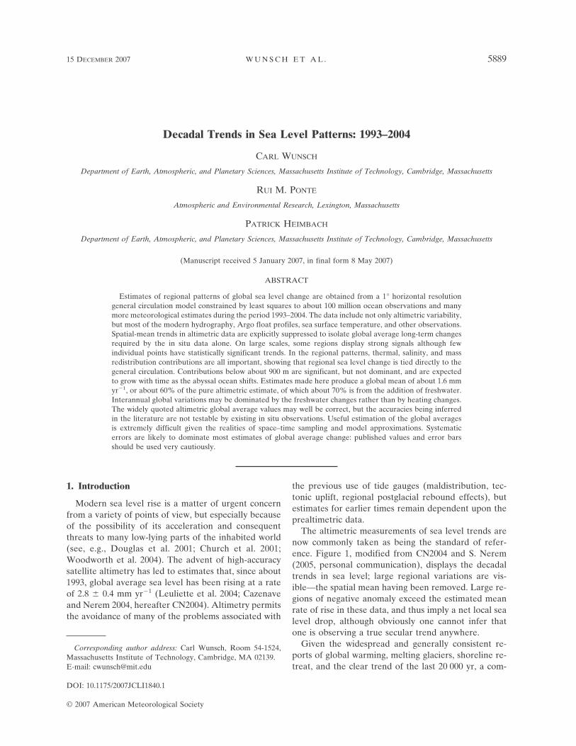
The altimetric measurements of sea level trends arenow commonly taken as being the standard of refer-ence. Figure 1, modified from CN2004 and S. Nerem(2005, personal communication), displays the decadaltrends in sea level; large regional variations are vis-ible—the spatial mean having been removed. Large re-gions of negative anomaly exceed the estimated meanrate of rise in these data, and thus imply a net local sealevel drop, although obviously one cannot infer thatone is observing a true secular trend anywhere.

Given the widespread and generally consistent re-ports of global warming, melting glaciers, shoreline re-treat, and the clear trend of the last 20 000 yr, a com-

Corresponding author address: Carl Wunsch, Room 54-1524,Massachusetts Institute of Technology, Cambridge, MA 02139.E-mail: [email protected]

15 DECEMBER 2007 W U N S C H E T A L . 5889

DOI: 10.1175/2007JCLI1840.1

© 2007 American Meteorological Society

JCLI4362

pelling inference is that global-mean sea level is rising.Because the altimetric values are so widely quoted, it isdesirable to buttress the values through independentmeans. Furthermore, obtaining a clear partitioning be-tween warming and the addition of freshwater to theocean has remained elusive, and the spatial patterns ofrise and fall are very complex.

Determining global and regional sea level shiftswould appear to be a reasonably straightforward pro-cess of forming averages of temperature and salinitymeasurements and then computing trends. In practice,almost no aspect of this problem is simple, and calcu-lations with known accuracy are very difficult.

a. Some preliminary numerics

It is useful to begin by setting out some order ofmagnitude values involved in studying sea level changeswhether from primarily data-based or model-based re-sults, or from a combination of the two. Suppose, asseems reasonable, that annual global-mean sea levelchange (positive or negative) is of order 1 mm yr�1. Themean ocean depth is h0 � 3800 m. Thus the volume ormass adjustment is O(10�3/3800) � 3 � 10�7 yr�1. Auseful rule of thumb is that in making estimates ofsignals, one should aim for a precision of better than10% of the expected signal. If GCMs or data are to beused to study global sea level change, one must there-fore aim for precisions in oceanic volume change oforder 10�8 yr�1. Whether such accuracies are now at-tainable remains to be seen.

Alternatively, suppose one seeks to use in situ mea-surements of temperature and salinity to estimateocean warming/freshening changes (negative warmingsand freshenings are included). A linearized equation ofstate, which is a useful approximation (see, e.g., Gille2004) is

� � ��1 � �T � �S�, �1�

where � 1.7 � 10�4 K�1, � 7.6 � 10�4, � � 1029,and T and S are temperature and salinity. For an orderof magnitude, suppose the ocean were fully mixed intemperature and salinity. Then (e.g., Patullo et al. 1955)a pure temperature change gives rise to a “thermo-steric” height change of

hT � ��Th0. �2�

A 1 mm yr�1 thermosteric change thus requires detect-ing an annual volume mean temperature change ofabout 1.5 � 10�3 °C yr�1.

Suppose, instead, that there is no temperaturechange, but that hm � 1 mm yr�1 of freshwater is addedor removed by glacial or groundwater storage changes(note that hm is not the “halosteric” change, which isdefined differently; see below). Then the salinitychange is

�S � �S0

hm

h0, �3�

where S0 � 35 is the initial average salinity on the prac-tical salinity scale. Thus �S � 10�5 yr�1.

FIG. 1. Twelve-year (1993–2004) trend in sea level (mm yr�1; updated from CN2004) asdetermined directly from the TOPEX/Poseidon altimetric data. An area-weighted spatialmean of 2.8 mm yr�1 was removed prior to plotting for direct comparison with the modelresults. Missing data areas show as white, as do a few obvious areas offscale in the negativedirection.

5890 J O U R N A L O F C L I M A T E VOLUME 20

Fig 1 live 4/C

Can one measure annual mean changes in tempera-ture and salinity with these magnitudes, again with thehope of having a precision 10 times better?

One further set of values is useful for context. Green-house gas heating is supposed (e.g., Hansen et al. 2005;Pierce et al. 2006) to be of order 1 W m�2. If thisamount of heat enters or leaves the ocean, the sea levelchange is about 1.3 mm yr�1. To infer from externalforcing that sea level has changed by 1 mm yr�1 re-quires an estimated heating change of 0.8 W m�2, againwith a goal of a precision 10 times better. If a value atone time is known with a standard error of , then thetemporal difference of values—assumed independent—would have a standard error of �2 and tests of sta-tistical significance require use of these numbers.

There are some important added complications inworking at these accuracies, some of which are taken upbelow. Consider here only that the equation of state issignificantly nonlinear (e.g., Jackett and McDougall1995) and at the millimeter level the linearized equa-tion of state is not sufficiently accurate. The cross termsof temperature and salinity plus the nonlinear tempera-ture terms have to be included, and the equation ofstate is needed to infer the thermal and haline changes.The latter (Munk 2003) is particularly troublesome be-cause an additional factor (the “Munk multiplier”) ofabout 37 is required to convert the so-called halostericchange into the desired mass change hm.

It is not clear at this stage whether the accuraciessuggested here are easy or difficult to achieve. If theyare challenging, an obvious strategy is to look forchanges over, for example, a decade, in which the 1 mmyr�1 translates into a much more easily measurable, butstill very difficult, 10 mm decade�1 with equivalentlarger changes in temperature and salinity. This strat-egy is reasonable and even practical, but it raises ques-tions, taken up later, as to whether systematic errors inmeasurements or models do not also grow at similarrates over a decade. Do signal-to-noise ratios increasewith time? Although the estimates described here rep-resent only the 12-yr period 1993–2004, most of thedifficulties encountered and described apply also to cal-culations made for arbitrarily long intervals with evenfewer data. Thus the inferences in the literature forother, usually longer, periods are briefly discussed hereas well.

b. An approach

Determination of accurate spatial averages doesprove difficult, and this paper is thus divided into twoparts. In the first, using nearly all of the extant tem-perature and salinity, altimetric, and other data avail-able globally from 1992 to 2004, we discuss the regional

variability in sea level and its contributing factors usinga dynamically consistent general circulation model. It isfound, as in Fig. 1, that regional variations are muchlarger than the expected global-mean values, thus mucheasier to determine, and so the system is inherentlynoisy. This noise is important in understanding the ac-curacy with which global-mean trends can be deter-mined, and thus in the second part of the paper, we turnto a brief, not very conclusive, discussion of the calcu-lations of the global averages.

The framework for our discussion is the Estimatingthe Circulation and Climate of the Ocean–GlobalOcean Data Assimilation Experiment (ECCO-GODAE)state estimation machinery discussed by Wunsch andHeimbach (2007) and Köhl et al. (2007). In essence, theoceanic general circulation model at 1° horizontal reso-lution with 23 vertical layers has been fit in a weighted,nonlinear, least squares sense to the global ocean ob-servations. The model is an evolved version of that de-scribed by Marshall et al. (1997; the MITgcm), and anumber of solutions to the least squares fit requirementnow exist, varying in the details of how the model wasconfigured, the duration, the particular data, and by theway in which the data were weighted in an overall misfit(objective or cost) function. A related effort is that ofCarton et al. (2005) who used a much more limiteddataset and a simpler optimization method that neednot produce a dynamically consistent time evolution.Wenzel and Schröter (2007) describe a calculation inspirit somewhat like this one, although using a muchsmaller dataset than ours.1

These approaches differ fundamentally from a num-ber of pure “forward” modeling simulations of oceanicheat uptake (e.g., Hansen et al. 2005; Pierce et al. 2006)in that the comparison of the model with the datasetsis here fully quantitative, any misfit being explicitlydetermined point by point, data type by data type.Pierce et al. (2006) note that among various models,simulated regional heat exchanges with the atmospherecan differ by up to factors of 8, and it is essential todetermine whether any of these models is inconsistentwith available observations.

An important conceptual point, and the source ofsome confusion, is that the results displayed here arefrom the unconstrained calculation by a forward model.

1 Köhl et al. (2007) discuss sea level changes in a previousECCO solution (v1.69) where the model configuration was some-what different, the data duration was shorter, and the misfit func-tion weights were also distinct. The process of model improve-ment and increased understanding of data errors is an asymptoticprocess, so that a definitive estimate will probably never be avail-able, only improving ones.


Before the model is run to produce the present results,it is first least squares fit to the data, as described, byadjusting its parameters (surface forcing, initial condi-tions, and in some experimental runs, interior mixingcoefficients, etc.). Using those adjusted parameters, themodel is then run forward in time, as in any ordinarymodel simulation, free of any constraints. This ap-proach contrasts with some other methods (e.g., in mostweather prediction systems using “assimilation”) wherethe model is adjusted “on the fly” in the forward cal-culation, forcing it by various means toward the obser-vations, and thus introducing unphysical temporalshifts. Because the datasets are comparatively thin dur-ing 1992, and there are indications of remaining startingtransients during that year, results here are stated forthe period 1993–2004.

To the extent that a least squares solution has beenobtained, it depends directly upon the weights assignedto the different data types. To put it another way, thenature and structure of the solution depends upon theerrors estimated for the data and for the model, whichtogether determine the extent to which the solution ispermitted to misfit. With too large a misfit, one isthrowing away useful, probably essential, information;too small a misfit implies one is fitting noise. The im-portance of using accurate error estimates is exempli-fied by the recent withdrawal of the Lyman et al. (2006)inference of an upper ocean cooling, 2003–05, upon thediscovery of a systematic error in much of their data(Willis et al. 2007), and the discussion by Gouretski andKoltermann (2007) of systematic biases in XBTdatasets.

2. The regional estimate

The ECCO-GODAE solutions used here (see Wunschand Heimbach 2007) employ approximately 100 millionoceanographic data constraints and about two billionmeteorological forcing variables (see Table 1). As in allleast squares problems, every one of them requires aweight, but only a brief summary of the weighting ispossible here. For present purposes, estimates of theerrors in the main data types include those for altimetry(see Fu and Cazenave 2001), summarized by Ponte etal. (2007), in the hydrography and Argo data by Forgetand Wunsch (2007), in the geoid and time-mean altim-etry by Stammer et al. (2007), and the meteorologicalvariables appearing in the control vector and taken ini-tially from the National Centers for EnvironmentalPrediction–National Center for Atmospheric Research(NCEP–NCAR) reanalysis of Kalnay et al. (1996). Inthis paper, the global-mean trends have been removedfrom all altimetric datasets, and as described later, themeteorological fields of freshwater and enthalpy fluxhave been subject to global balance constraints.

Although the calculations are ongoing and solutionsslowly changing, the least squares estimate is nowstable and provides generally acceptable misfits (asmeasured by estimated model and data errors) over thegreat bulk of the ocean and the entire period. Excep-tions do exist, and we make no claim to be “correct,”merely that we are going to use a “best-existing-estimate,” solution version v2.216 (the 216 is the itera-tion number; leading 2 refers to the model and dataversion). A variety of experiments with boundary con-

TABLE 1. Listing of the approximate numbers of most observational data types used to constrain the model. These values are onlyapproximate because some derived quantities such as the NCEP–NCAR reanalysis and the hydrographic climatologies are far removedfrom direct observations. In the least squares calculation, each of these constraints requires an explicit weight, although in this version,bottom topography is not in the control vector and is effectively given infinite weight (as though perfect). Further data, e.g., tide gauges,have been withheld and are used as tests of system skill.

Meteorological variables No.

NCEP–NCAR (6-hourly wind stress, buoyancy flux, shortwave/longwave radiation) 2.1 � 109

Oceanographic variables

Altimetry (TOPEX, Jason-1, GFO, ERS-1/2, Envisat) 3.3 � 107

XBT 1.9 � 107

Argo profile temperature and salinity 2.1 � 107

CTD temperature and salinity 2 � 106

Hydrographic climatologies 1.6 � 107

Sea surface temperature 5.3 � 106

Tropical Rainfall Measuring Mission (TRMM) Microwave Imager (TMI) temperatures 1.5 � 106

Gravity Recovery and Climate Experiment (GRACE) geoid 57 600Bottom topography 57 600Quick Scatterometer (QuikSCAT) winds 1.0 � 107

Approximate No. of oceanographic observations 1.1 � 108

Approximate No. of total weighted values 2.11 � 109


ditions, data weights, and hundreds of iterations pro-duces generally similar results for sea level change.Nonetheless, as with any large nonlinear optimizationcalculation, one cannot categorically rule out the ap-pearance of qualitative changes as iterations proceed—unlikely as that now appears. Efforts to improve theestimate will necessarily continue indefinitely.

The present model uses the Boussinesq approxima-tion with a virtual salt flux boundary condition at thesea surface. Although it is an issue primarily for thediscussion of global-mean sea level rise, we note here(see Table 2) that at least six surface boundary condi-tions are in use with ocean GCMs. Later reference willbe made to this table.

In a Boussinesq approximation model (e.g., Great-batch 1994), volume is conserved; the global average

anomaly of elevation, �(t), must vanish; and bottompressure can fictitiously vary from net heating or cool-ing, for which a correction must be made. Regionalresults here use only the Boussinesq approximation el-evations and bottom pressures without global averagecorrection. The later global-mean discussion requires adifferent treatment.

a. Regional results

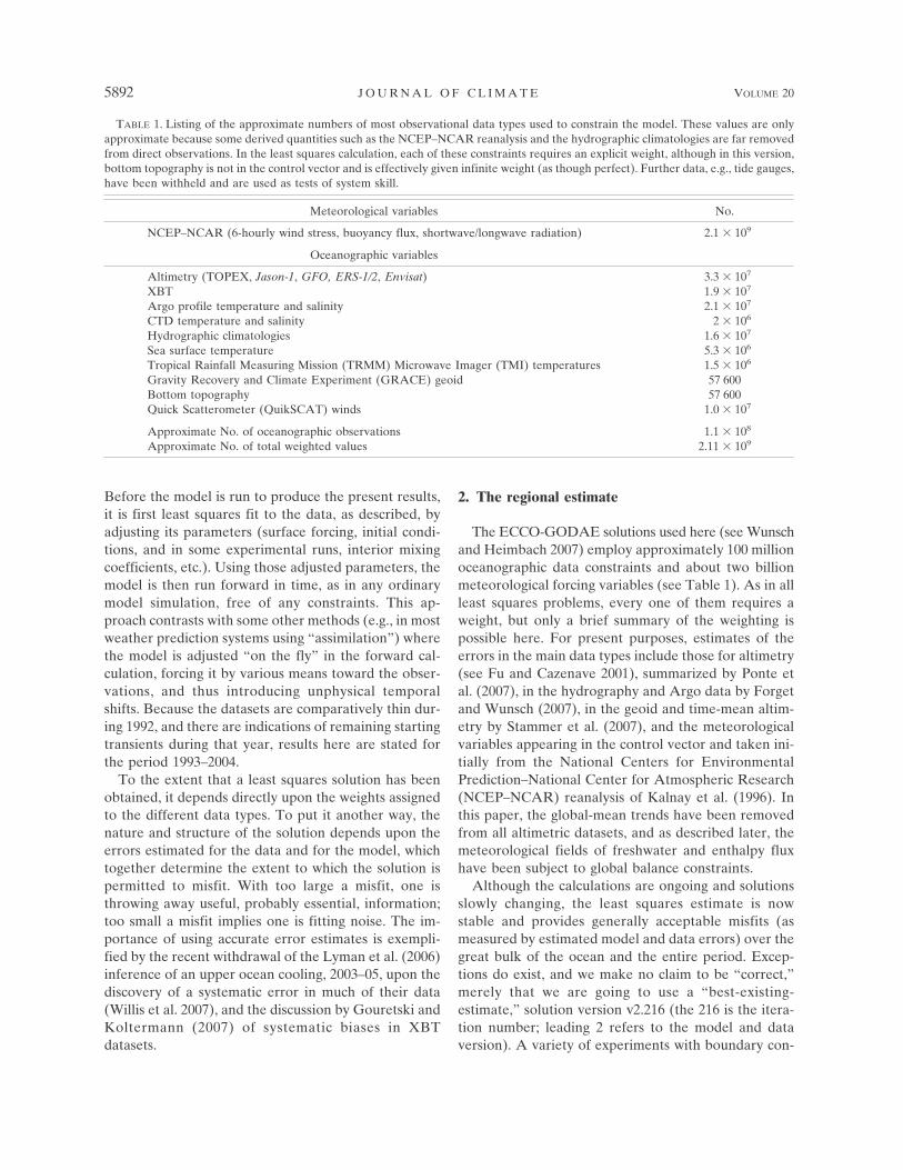
Figure 2 shows the local trends in relative sea surfaceheight, �, with its standard error in Fig. 3, as deter-mined prognostically from ECCO-GODAE v2.216.Figure 4 displays the trends in the model prior to opti-mization [i.e., without effects of data constraints and asdescribed by Wunsch and Heimbach (2007)]. Compari-son between the two fields reveals substantial differ-

FIG. 2. Sea level trend (m yr�1) from solution v2.216 of the model computed over 1993–2004and directly comparable to Fig. 1 apart from the greater area used. It is important that thisfigure be used with the partial error estimate shown in Fig. 3, particularly concerning theregion around Antarctica where few data of any kind are available. (�ere � is defined as theprognostic value appearing in boundary condition 2 of Table 2, and in the Boussinesq ap-proximation has zero spatial average.)

TABLE 2. Six surface boundary condition combinations in wide use in oceanic GCMs. These differ in the way the continuity andsalinity conservation equations are used. Here h � h0 � �, where h0 is the unperturbed total depth. Definitions are RIGLID—rigid lid;VSF—virtual salt flux; LIN FS—linearized free surface; VFW—virtual freshwater flux; NLFS—nonlinear free surface; RFW—realfreshwater flux. See P. Heimbach and J.-M. Campin (2006, unpublished manuscript). Unfortunately, determination of the slight massaddition to the ocean depends directly upon the accuracy of these representations. Condition 6 is the desired form, and the only onenot placing an inappropriate source into the salinity conservation equation. Here, the freshwater results from conditions 2 and 6 arequite close, but 2, which we use, is capable of generating spurious circulations (see Huang 1993).

No. Continuity equation Tracer conservation equation Freshwater input Label

1 � · h0v � 0 �t(h0S) � � · h0Sv � �P · S0 Virtual salt flux RIGLID � VSF2 �t� � � · h0v � 0 �t(h0S) � � · h0Sv � �P · S0 Virtual salt flux LINFS � VSF3 �t� � � · h0v � P �t(h0S) � � · h0Sv � �P · S Virtual freshwater flux LINFS � VFW4 �t� � � · h0v � P �t(h0S) � � · h0Sv � �P · S0 Approx virtual freshwater flux LINFS � A-VFW5 �t� � � · hv � 0 �t(hS) � � · hSv � �P · S0 Virtual salt flux NLFS � VSF6 �t� � � · hv � P �t(hS) � � · hSv � 0 Real freshwater flux NLFS � RFW


Fig 2 live 4/C

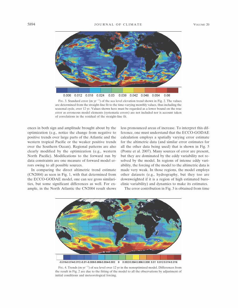
ences in both sign and amplitude brought about by theoptimization (e.g., notice the change from negative topositive trends over large parts of the Atlantic and thewestern tropical Pacific or the weaker positive trendsover the Southern Ocean). Regional patterns are alsoclearly modified by the optimization (e.g., westernNorth Pacific). Modifications to the forward run bydata constraints are one measure of forward model er-rors owing to all possible sources.

In comparing the direct altimetric trend estimate(CN2004) as seen in Fig. 1, with that determined fromthe ECCO-GODAE model, one can see gross similari-ties, but some significant differences as well. For ex-ample, in the North Atlantic the CN2004 result shows

less pronounced areas of increase. To interpret this dif-ference, one must understand that the ECCO-GODAEcalculation employs a spatially varying error estimatefor the altimetric data (and similar error estimates forall the other data being used) that is shown in Fig. 5(Ponte et al. 2007). Many sources of error are present,but they are dominated by the eddy variability not re-solved by the model. In regions of intense eddy vari-ability, the forcing of the model to the altimetric data ismade very weak. In those regions, the model employsother datasets (e.g., hydrography, but they too aredownweighted if it is a region of high estimated baro-clinic variability) and dynamics to make its estimates.

The error contribution in Fig. 3 is obtained from time

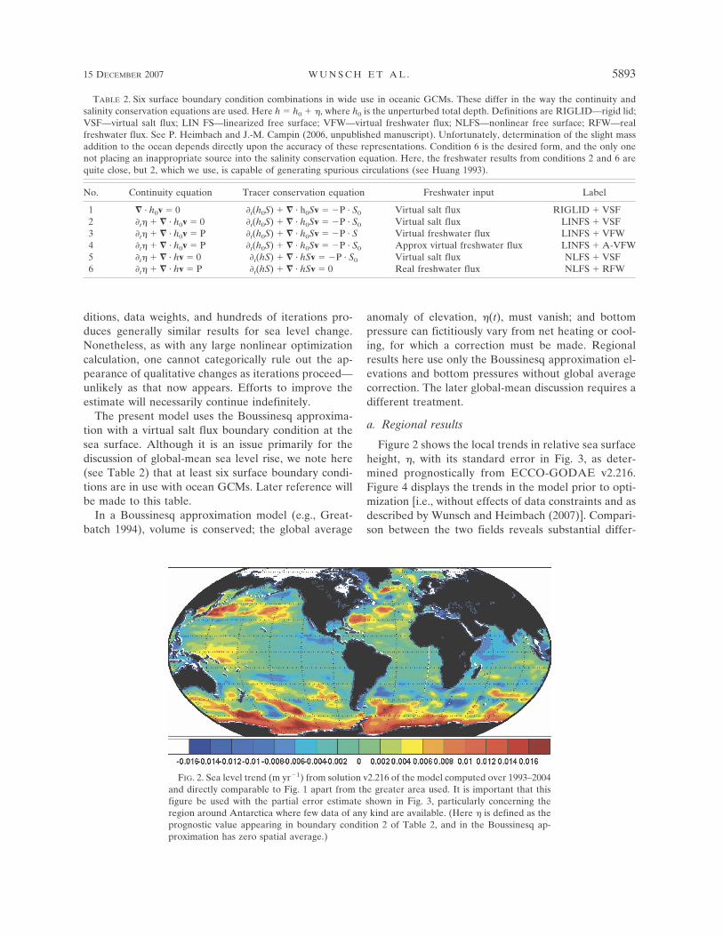
FIG. 3. Standard error (m yr�1) of the sea level elevation trend shown in Fig. 2. The valuesare determined from the straight-line fit to the time-varying monthly values, thus including theseasonal cycle, over 12 yr. Values shown here must be regarded as a lower bound on the trueerror as erroneous model elements (systematic errors) are not included nor is account takenof correlations in the residual of the straight-line fit.

FIG. 4. Trends (m yr�1) of sea level over 12 yr in the nonoptimized model. Differences fromthe result in Fig. 2 are due to the fitting of the model to all the observations by adjustment ofinitial conditions and meteorological forcing.


Fig 3 and 4 live 4/C

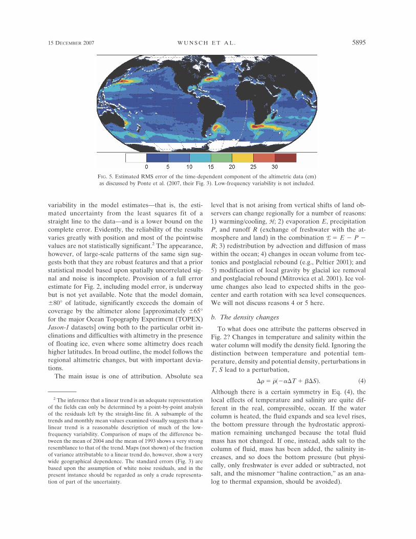
variability in the model estimates—that is, the esti-mated uncertainty from the least squares fit of astraight line to the data—and is a lower bound on thecomplete error. Evidently, the reliability of the resultsvaries greatly with position and most of the pointwisevalues are not statistically significant.2 The appearance,however, of large-scale patterns of the same sign sug-gests both that they are robust features and that a priorstatistical model based upon spatially uncorrelated sig-nal and noise is incomplete. Provision of a full errorestimate for Fig. 2, including model error, is underwaybut is not yet available. Note that the model domain,�80° of latitude, significantly exceeds the domain ofcoverage by the altimeter alone [approximately �65°for the major Ocean Topography Experiment (TOPEX)Jason-1 datasets] owing both to the particular orbit in-clinations and difficulties with altimetry in the presenceof floating ice, even where some altimetry does reachhigher latitudes. In broad outline, the model follows theregional altimetric changes, but with important devia-tions.

The main issue is one of attribution. Absolute sea

level that is not arising from vertical shifts of land ob-servers can change regionally for a number of reasons:1) warming/cooling, H ; 2) evaporation E, precipitationP, and runoff R (exchange of freshwater with the at-mosphere and land) in the combination E � E � P �R; 3) redistribution by advection and diffusion of masswithin the ocean; 4) changes in ocean volume from tec-tonics and postglacial rebound (e.g., Peltier 2001); and5) modification of local gravity by glacial ice removaland postglacial rebound (Mitrovica et al. 2001). Ice vol-ume changes also lead to expected shifts in the geo-center and earth rotation with sea level consequences.We will not discuss reasons 4 or 5 here.

b. The density changes

To what does one attribute the patterns observed inFig. 2? Changes in temperature and salinity within thewater column will modify the density field. Ignoring thedistinction between temperature and potential tem-perature, density and potential density, perturbations inT, S lead to a perturbation,

�� T � ��S�. �4�

Although there is a certain symmetry in Eq. (4), thelocal effects of temperature and salinity are quite dif-ferent in the real, compressible, ocean. If the watercolumn is heated, the fluid expands and sea level rises,the bottom pressure through the hydrostatic approxi-mation remaining unchanged because the total fluidmass has not changed. If one, instead, adds salt to thecolumn of fluid, mass has been added, the salinity in-creases, and so does the bottom pressure (but physi-cally, only freshwater is ever added or subtracted, notsalt, and the misnomer “haline contraction,” as an ana-log to thermal expansion, should be avoided).

2 The inference that a linear trend is an adequate representationof the fields can only be determined by a point-by-point analysisof the residuals left by the straight-line fit. A subsample of thetrends and monthly mean values examined visually suggests that alinear trend is a reasonable description of much of the low-frequency variability. Comparison of maps of the difference be-tween the mean of 2004 and the mean of 1993 shows a very strongresemblance to that of the trend. Maps (not shown) of the fractionof variance attributable to a linear trend do, however, show a verywide geographical dependence. The standard errors (Fig. 3) arebased upon the assumption of white noise residuals, and in thepresent instance should be regarded as only a crude representa-tion of part of the uncertainty.

FIG. 5. Estimated RMS error of the time-dependent component of the altimetric data (cm)as discussed by Ponte et al. (2007, their Fig. 3). Low-frequency variability is not included.


Fig 5 live 4/C

The “mass” height hm is the contribution from theaddition or subtraction of freshwater.3 As Munk (2003)emphasized, it is not the same as the so-called halostericheight hS, which is the apparent expansion or contrac-tion of the water column from a change in the averagesalinity (Patullo et al. 1955),

hS ��S

1 � �S0h0 � ��Sh0. �5�

The relationship between the salinity change and massheight is given by Eq. (3), which implies

hm �hS

�S0,

where the “Munk multiplier,” 1/S0 � 36.7, is a largenumber.

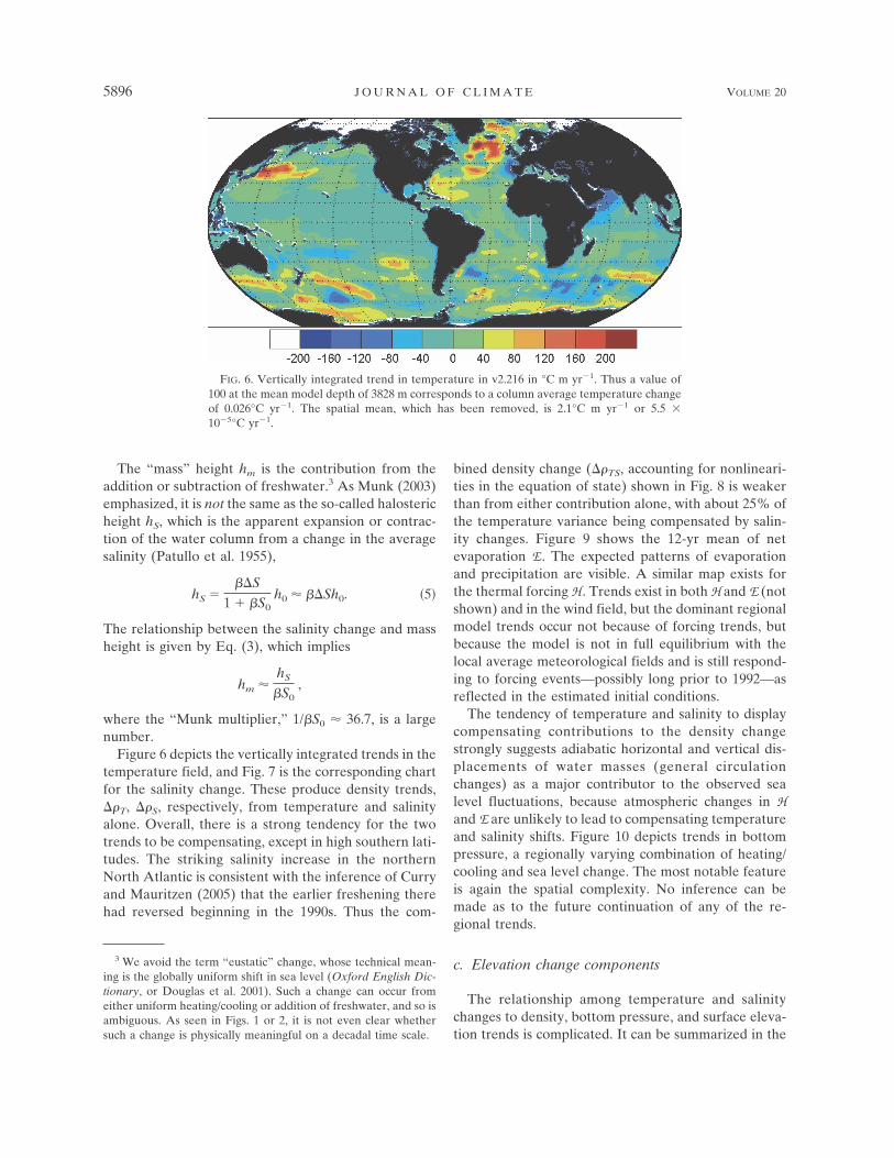
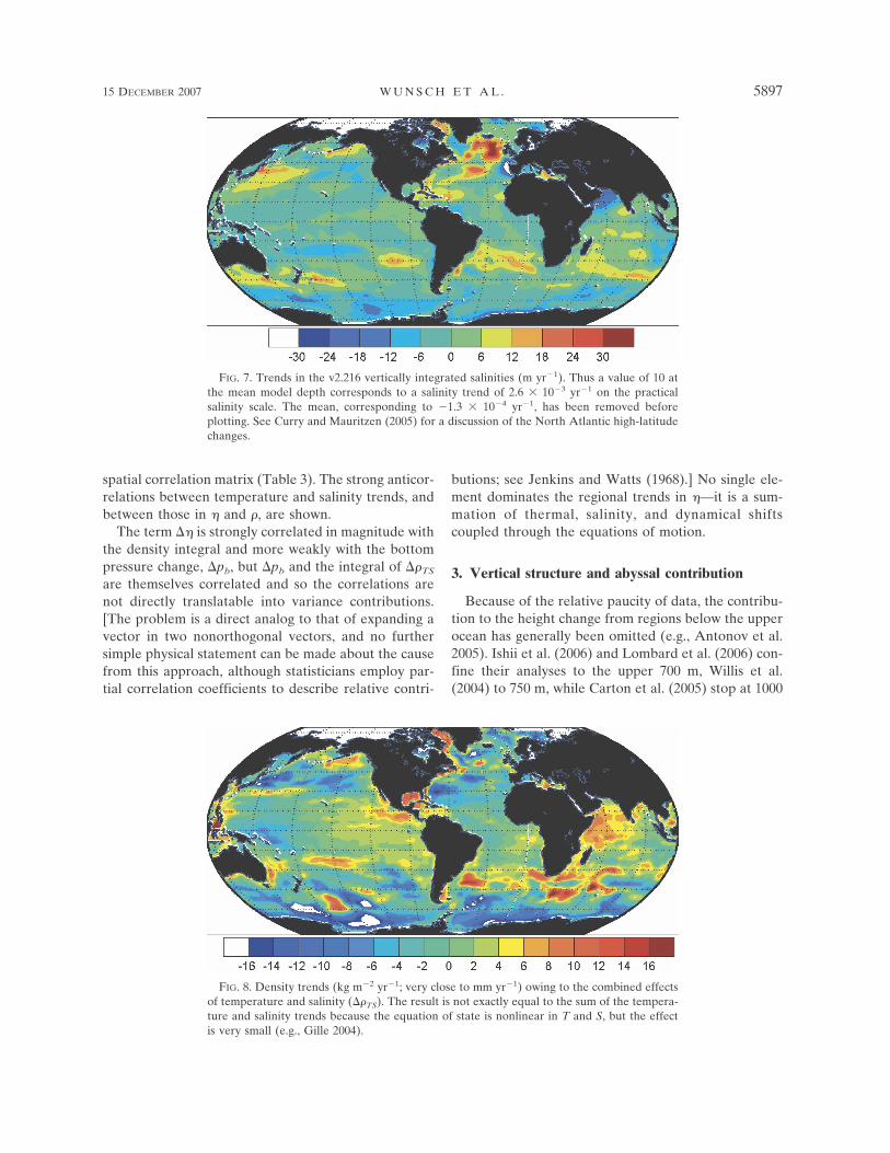
Figure 6 depicts the vertically integrated trends in thetemperature field, and Fig. 7 is the corresponding chartfor the salinity change. These produce density trends,��T, ��S, respectively, from temperature and salinityalone. Overall, there is a strong tendency for the twotrends to be compensating, except in high southern lati-tudes. The striking salinity increase in the northernNorth Atlantic is consistent with the inference of Curryand Mauritzen (2005) that the earlier freshening therehad reversed beginning in the 1990s. Thus the com-

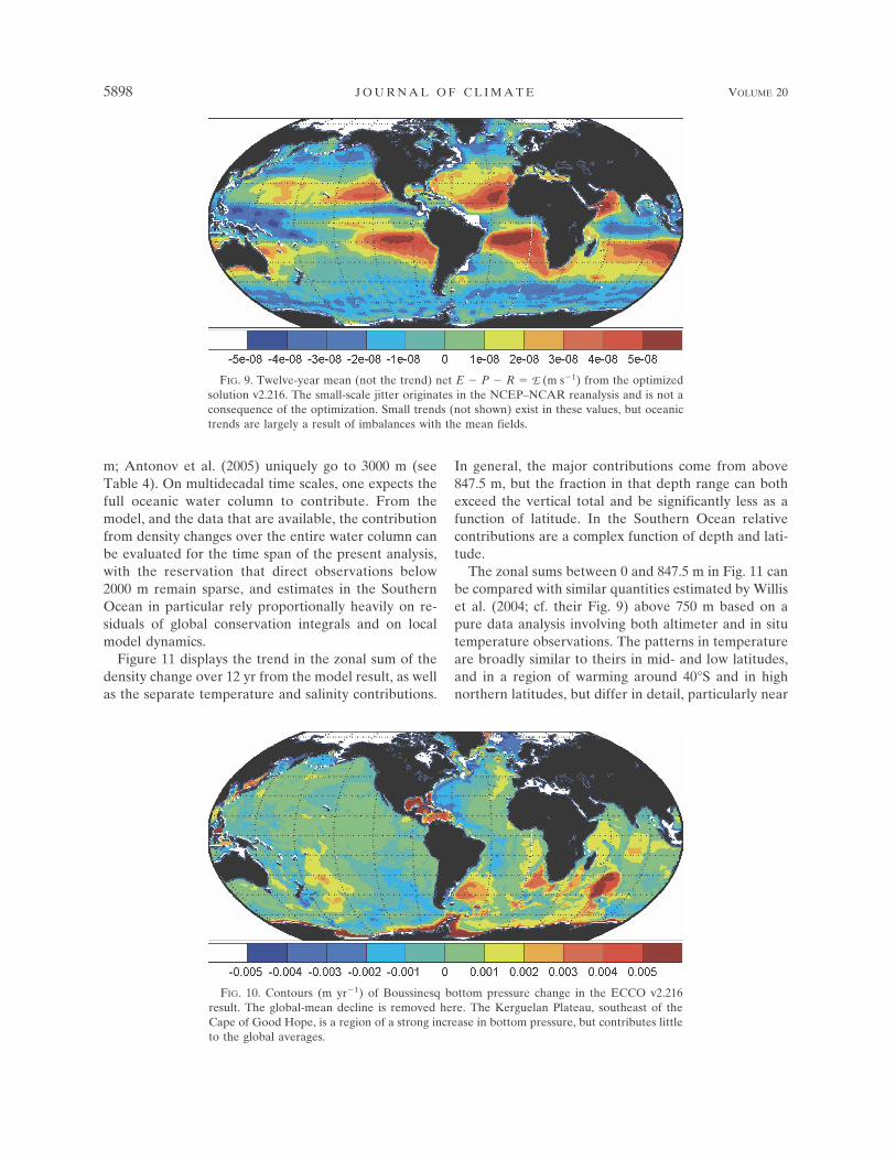
bined density change (��TS, accounting for nonlineari-ties in the equation of state) shown in Fig. 8 is weakerthan from either contribution alone, with about 25% ofthe temperature variance being compensated by salin-ity changes. Figure 9 shows the 12-yr mean of netevaporation E . The expected patterns of evaporationand precipitation are visible. A similar map exists forthe thermal forcing H . Trends exist in both H and E (notshown) and in the wind field, but the dominant regionalmodel trends occur not because of forcing trends, butbecause the model is not in full equilibrium with thelocal average meteorological fields and is still respond-ing to forcing events—possibly long prior to 1992—asreflected in the estimated initial conditions.

The tendency of temperature and salinity to displaycompensating contributions to the density changestrongly suggests adiabatic horizontal and vertical dis-placements of water masses (general circulationchanges) as a major contributor to the observed sealevel fluctuations, because atmospheric changes in Hand E are unlikely to lead to compensating temperatureand salinity shifts. Figure 10 depicts trends in bottompressure, a regionally varying combination of heating/cooling and sea level change. The most notable featureis again the spatial complexity. No inference can bemade as to the future continuation of any of the re-gional trends.

c. Elevation change components

The relationship among temperature and salinitychanges to density, bottom pressure, and surface eleva-tion trends is complicated. It can be summarized in the

3 We avoid the term “eustatic” change, whose technical mean-ing is the globally uniform shift in sea level (Oxford English Dic-tionary, or Douglas et al. 2001). Such a change can occur fromeither uniform heating/cooling or addition of freshwater, and so isambiguous. As seen in Figs. 1 or 2, it is not even clear whethersuch a change is physically meaningful on a decadal time scale.

FIG. 6. Vertically integrated trend in temperature in v2.216 in °C m yr�1. Thus a value of100 at the mean model depth of 3828 m corresponds to a column average temperature changeof 0.026°C yr�1. The spatial mean, which has been removed, is 2.1°C m yr�1 or 5.5 �10�5°C yr�1.


Fig 6 live 4/C

spatial correlation matrix (Table 3). The strong anticor-relations between temperature and salinity trends, andbetween those in � and �, are shown.

�he term �� is strongly correlated in magnitude withthe density integral and more weakly with the bottompressure change, �pb, but �pb and the integral of ��TS

are themselves correlated and so the correlations arenot directly translatable into variance contributions.[The problem is a direct analog to that of expanding avector in two nonorthogonal vectors, and no furthersimple physical statement can be made about the causefrom this approach, although statisticians employ par-tial correlation coefficients to describe relative contri-

butions; see Jenkins and Watts (1968).] No single ele-ment dominates the regional trends in �—it is a sum-mation of thermal, salinity, and dynamical shiftscoupled through the equations of motion.

3. Vertical structure and abyssal contribution

Because of the relative paucity of data, the contribu-tion to the height change from regions below the upperocean has generally been omitted (e.g., Antonov et al.2005). Ishii et al. (2006) and Lombard et al. (2006) con-fine their analyses to the upper 700 m, Willis et al.(2004) to 750 m, while Carton et al. (2005) stop at 1000

FIG. 7. Trends in the v2.216 vertically integrated salinities (m yr�1). Thus a value of 10 atthe mean model depth corresponds to a salinity trend of 2.6 � 10�3 yr�1 on the practicalsalinity scale. The mean, corresponding to �1.3 � 10�4 yr�1, has been removed beforeplotting. See Curry and Mauritzen (2005) for a discussion of the North Atlantic high-latitudechanges.

FIG. 8. Density trends (kg m�2 yr�1; very close to mm yr�1) owing to the combined effectsof temperature and salinity (��TS). The result is not exactly equal to the sum of the tempera-ture and salinity trends because the equation of state is nonlinear in T and S, but the effectis very small (e.g., Gille 2004).


Fig 7 and 8 live 4/C

m; Antonov et al. (2005) uniquely go to 3000 m (seeTable 4). On multidecadal time scales, one expects thefull oceanic water column to contribute. From themodel, and the data that are available, the contributionfrom density changes over the entire water column canbe evaluated for the time span of the present analysis,with the reservation that direct observations below2000 m remain sparse, and estimates in the SouthernOcean in particular rely proportionally heavily on re-siduals of global conservation integrals and on localmodel dynamics.

Figure 11 displays the trend in the zonal sum of thedensity change over 12 yr from the model result, as wellas the separate temperature and salinity contributions.

In general, the major contributions come from above847.5 m, but the fraction in that depth range can bothexceed the vertical total and be significantly less as afunction of latitude. In the Southern Ocean relativecontributions are a complex function of depth and lati-tude.

The zonal sums between 0 and 847.5 m in Fig. 11 canbe compared with similar quantities estimated by Williset al. (2004; cf. their Fig. 9) above 750 m based on apure data analysis involving both altimeter and in situtemperature observations. The patterns in temperatureare broadly similar to theirs in mid- and low latitudes,and in a region of warming around 40°S and in highnorthern latitudes, but differ in detail, particularly near

FIG. 9. Twelve-year mean (not the trend) net E � P � R � E (m s�1) from the optimizedsolution v2.216. The small-scale jitter originates in the NCEP–NCAR reanalysis and is not aconsequence of the optimization. Small trends (not shown) exist in these values, but oceanictrends are largely a result of imbalances with the mean fields.

FIG. 10. Contours (m yr�1) of Boussinesq bottom pressure change in the ECCO v2.216result. The global-mean decline is removed here. The Kerguelan Plateau, southeast of theCape of Good Hope, is a region of a strong increase in bottom pressure, but contributes littleto the global averages.


Fig 9 live 4/C

20°N and S and in the absence here of the strong cool-ing they see at about 38°–50°N.

Figures 12 and 13 show the patterns of temperatureand salinity trends between 985 and 1750 m, and Figs.14 and 15 show the 985 m to the bottom trends over themodel duration and display the complexity of the

change even at depth. Omission of the ocean below themain thermocline does, for the 12-yr period, give a use-ful estimate of ongoing behavior, although there arequantitative errors. Whether that will remain true asglobal change continues and anomalies have time topenetrate the abyss remains to be seen. Figure 16 sug-gests significant warming in the Southern Ocean andalong the North Atlantic margin, roughly coincidingwith the position of the deep western boundary currentthere.

4. The spatial mean

We turn now to the problem of determining the glo-bal trend means, which as described in the introduction,are small residuals of large spatial and temporal varia-tions. Because of the difficulties with both datasets andmodels, much of the result here is inconclusive: thereliability of the global average estimates remainspoorly known. Appendix A contains a more extendeddiscussion of the many troublesome details.

A number of authors have grappled with the problem

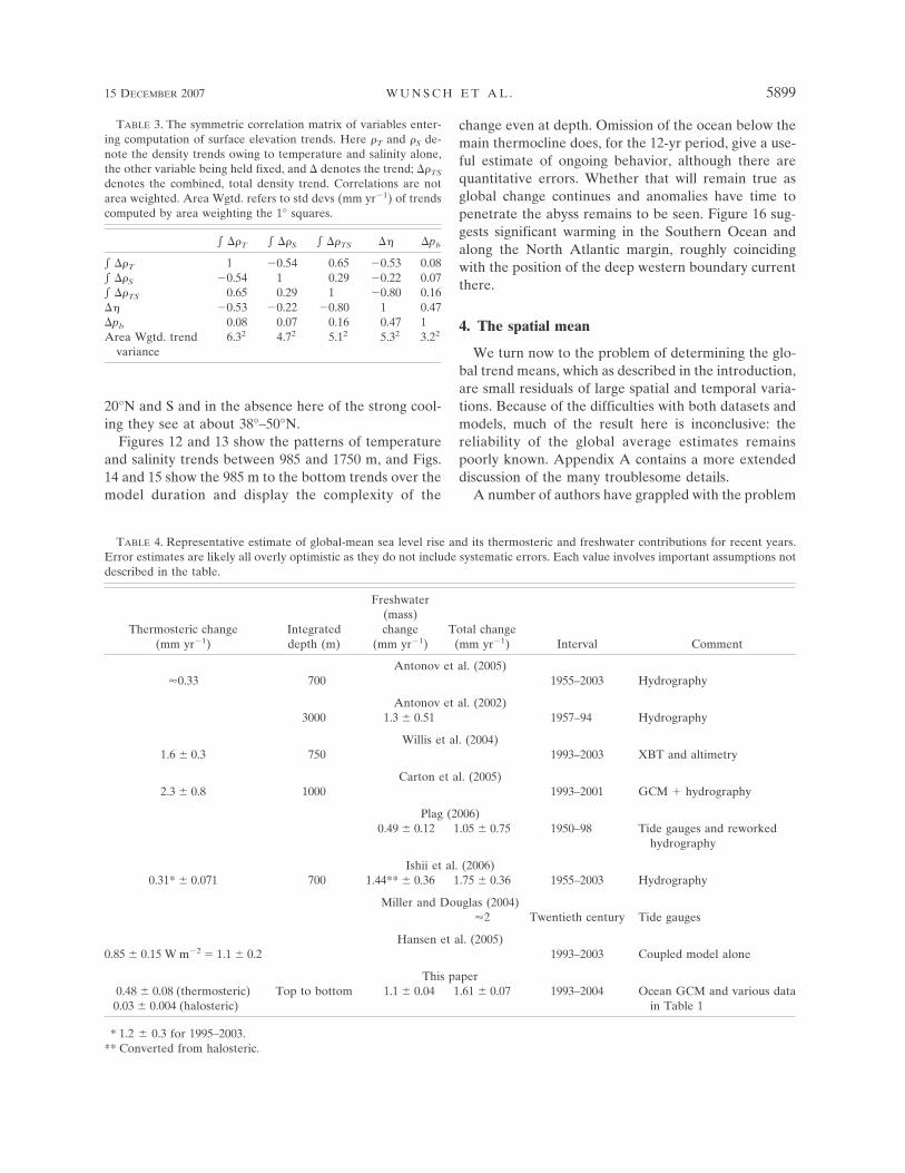
TABLE 4. Representative estimate of global-mean sea level rise and its thermosteric and freshwater contributions for recent years.Error estimates are likely all overly optimistic as they do not include systematic errors. Each value involves important assumptions notdescribed in the table.

Thermosteric change(mm yr�1)

Integrateddepth (m)

Freshwater(mass)change

(mm yr�1)Total change

(mm yr�1) Interval Comment

Antonov et al. (2005)�0.33 700 1955–2003 Hydrography

Antonov et al. (2002)3000 1.3 � 0.51 1957–94 Hydrography

Willis et al. (2004)1.6 � 0.3 750 1993–2003 XBT and altimetry

Carton et al. (2005)2.3 � 0.8 1000 1993–2001 GCM � hydrography

Plag (2006)0.49 � 0.12 1.05 � 0.75 1950–98 Tide gauges and reworked

hydrography

Ishii et al. (2006)0.31* � 0.071 700 1.44** � 0.36 1.75 � 0.36 1955–2003 Hydrography

Miller and Douglas (2004)�2 Twentieth century Tide gauges

Hansen et al. (2005)0.85 � 0.15 W m�2 � 1.1 � 0.2 1993–2003 Coupled model alone

This paper0.48 � 0.08 (thermosteric) Top to bottom 1.1 � 0.04 1.61 � 0.07 1993–2004 Ocean GCM and various data

in Table 10.03 � 0.004 (halosteric)

* 1.2 � 0.3 for 1995–2003.** Converted from halosteric.

TABLE 3. The symmetric correlation matrix of variables enter-ing computation of surface elevation trends. Here �T and �S de-note the density trends owing to temperature and salinity alone,the other variable being held fixed, and � denotes the trend; ��TS

denotes the combined, total density trend. Correlations are notarea weighted. Area Wgtd. refers to std devs (mm yr�1) of trendscomputed by area weighting the 1° squares.

� ��T � ��S � ��TS �� pb

� ��T 1 �0.54 0.65 �0.53 0.08� ��S �0.54 1 0.29 �0.22 0.07� ��TS 0.65 0.29 1 �0.80 0.16�� 0.53 �0.22 �0.80 1 0.47�pb 0.08 0.07 0.16 0.47 1Area Wgtd. trend

variance6.32 4.72 5.12 5.32 3.22


of determining the spatial means from in situ and alti-metric data (see Table 4). Here, existing estimates ofthe spatial means are referred to as “subglobal” to dis-tinguish them from the goal of truly global ones. Eventhe problem of forming an average, specifically oftrends, requires comment because almost all model av-erages are small residuals of fields with large fluctua-tions, and at least four different methods for computingthe averages can be considered (see appendix A). Theterminology of global averages must be used cautiouslyto avoid the implication that the ocean displays any-thing approaching a uniform linear trend (it plainlydoes not). The quotation of averages is simply anintuitively accessible surrogate for global fluid ocean-volume changes, however distributed, as measured incubic meters per year.

Each of the datasets (commonly tide gauges, altim-eters, hydrographic measurements) has troubling issuesof space–time sampling and of physical interpretation.Altimetric data (CN2004) are widely accepted as pro-viding the best available estimate of mean global sea

level rise, although errors in the time-varying compo-nents of altimetric datasets are complex and not whollyquantified. As summarized in appendix B, the majorsampling issues concern the cutoff at about 60°S fromorbital configuration or floating sea ice, and the possi-bility of trends in the long list of corrections made tothe data.

For hydrography, the major problems consist of thevery irregular space–time sampling, the bias toward theupper ocean, the seasonal cycle in sampling in the pres-ence of a strong seasonal signal, and the possibility ofsystematic errors as the technology for salinity, tem-perature, and depth determination changed over thelast 50 yr. Tide gauge problems have been widely dis-cussed (e.g., Douglas et al. 2001).

The models introduce a very large number of ap-proximations and errors, some connected with thedatasets and some connected to the numerics andphysical approximations. As noted in the introduction,a sea level change of 1 mm yr�1 in an ocean of meandepth near 4000 m implies a fractional volume or mass

FIG. 11. Zonal sums of the trends in vertical integrals of the (top) model density anomaly(kg m�2 yr�1), (middle) from temperature pattern alone, and (bottom) from salinity alone.Solid, black curve is the total top-to-bottom change. Dashed blue curve is the contributionfrom the main thermocline and above, red is from the thermocline to 1975 m, green is from1975 to 2450 m, and cyan is from 2450 to the maximum model depth. Where the dashed bluecurve is near the black, the ocean above about 850 m accounts for the entire change, althoughoften that occurs because temperature and salinity contributions tend to cancel at depth.Middle latitudes and parts of the Southern Ocean display significant deviations from upperocean dominance. For temperature note again that a negative density anomaly corresponds towarming.


Fig 11 live 4/C

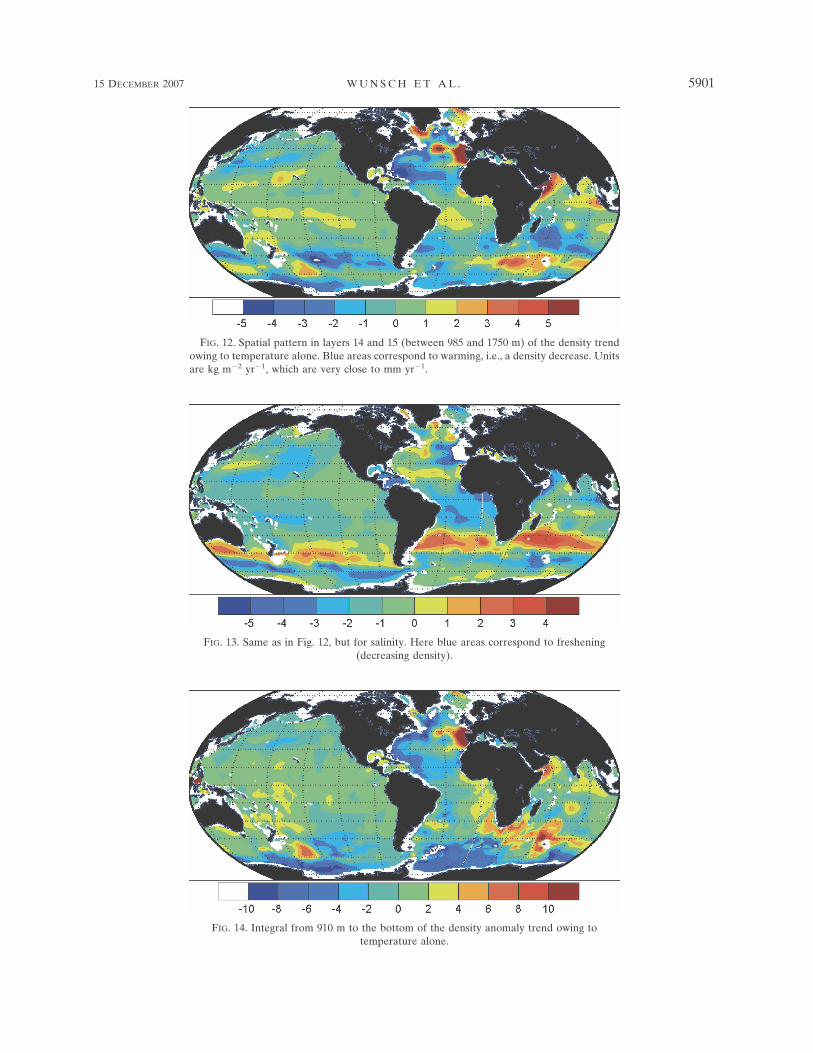
FIG. 12. Spatial pattern in layers 14 and 15 (between 985 and 1750 m) of the density trendowing to temperature alone. Blue areas correspond to warming, i.e., a density decrease. Unitsare kg m�2 yr�1, which are very close to mm yr�1.

FIG. 13. Same as in Fig. 12, but for salinity. Here blue areas correspond to freshening(decreasing density).

FIG. 14. Integral from 910 m to the bottom of the density anomaly trend owing totemperature alone.


Fig 12 13 and 14 live 4/C

change of 3 � 10�7 per year of integration time. De-termining whether such accuracies are now achievablewith a GCM leads one to examine a very long list ofapproximations made in any numerical model. Withoutclaiming to have a definitive answer, appendix C out-

lines some of the issues. Table 2 lists six different sur-face boundary conditions for salt and freshwater incommon use. Attempts here at using several of themshow that they can produce differences in apparent sealevel trends approaching an order of magnitude. Asappendix C discusses, we rely primarily upon the linearfreshwater/virtual salt flux formulation, as it was bothadjointable4 and produced consistent results for salin-ity, density, and sea level changes.

In the current Boussinesq approximation model, aconversion from volume conservation to mass conser-vation is required; this conversion (e.g., Greatbatch1994) is itself an approximation. Further references canbe found in appendix C. Because a Boussinesq modelproduces an elevation change � whose global mean isby definition zero, one must diagnose the global-meanchange �� as

�� pb � �� 6�

or

�� 1��h

0

��TS dz � 36.7��h

0

��S dz, �7�

where ��TS is the total density change, and ��S is thechange in density owing to salinity change alone. Thevalue 36.7 is the Munk multiplier, z � �h is the waterdepth, and � is a reference density (1029 kg m�3).

Most ocean GCMs, even if not optimized, are forcedby surface boundary conditions including net heating H,and net estimated evaporation minus precipitation mi-nus runoff E from the atmospheric reanalyses and

4 The model adjoint is used to carry out the least squares mini-mization. See Wunsch and Heimbach (2007).

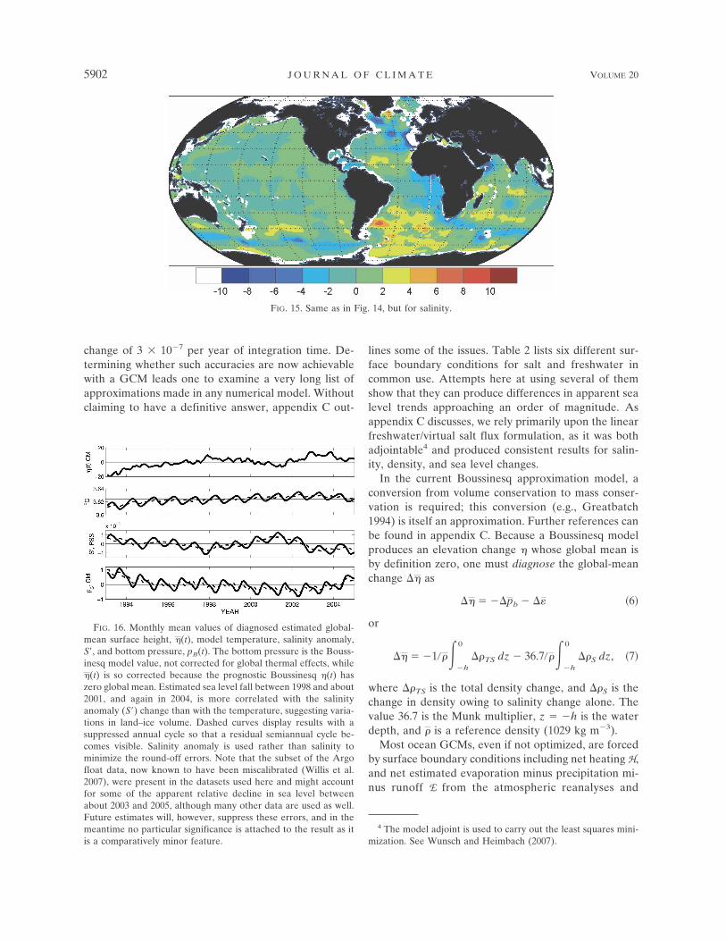
FIG. 15. Same as in Fig. 14, but for salinity.

FIG. 16. Monthly mean values of diagnosed estimated global-mean surface height, �(t), model temperature, salinity anomaly,S�, and bottom pressure, pB(t). The bottom pressure is the Bouss-inesq model value, not corrected for global thermal effects, while�(t) is so corrected because the prognostic Boussinesq �(t) haszero global mean. Estimated sea level fall between 1998 and about2001, and again in 2004, is more correlated with the salinityanomaly (S�) change than with the temperature, suggesting varia-tions in land–ice volume. Dashed curves display results with asuppressed annual cycle so that a residual semiannual cycle be-comes visible. Salinity anomaly is used rather than salinity tominimize the round-off errors. Note that the subset of the Argofloat data, now known to have been miscalibrated (Willis et al.2007), were present in the datasets used here and might accountfor some of the apparent relative decline in sea level betweenabout 2003 and 2005, although many other data are used as well.Future estimates will, however, suppress these errors, and in themeantime no particular significance is attached to the result as itis a comparatively minor feature.


Fig 15 live 4/C

where runoff is taken from Fekete et al. (2002). Avail-able reanalyses are derived from weather forecast mod-els that do not impose global balances for freshwaterand heat. In addition, the runoff component from melt-ing glacial ice is subject to great controversy, includingeven its sign (e.g., Cazenave 2006). Imbalances in sur-face forcing can easily give rise to systematic errors ofthe magnitude of the signal we seek. Other issues, suchas the absence of geothermal heating, become trouble-some over the longer time scales.

Estimation-system global means

The ECCO-GODAE global-mean estimates are de-pendent approximately equally on the assumptions ofthe absence of spurious trends in model dynamics/kinematics, and in the various datasets. We here willstate the estimated global trends, with formal errorbars, but we believe the greatest uncertainty in the re-sults lies with the possibility of systematic errors in bothdata and model, and for which we lack quantitativeestimates. Formal error bars, referring only to the ex-pected stochastic errors, are commonly quoted asthough they represent total uncertainties, and they areprobably misleadingly optimistic.

In the ECCO-GODAE calculations, the spatial-mean sea level trend was removed from the altimetricdatasets. [The area-averaged trend in the EuropeanRemote Sensing Satellite-1 and -2 (ERS-1, -2)/Environ-mental Satellite (Envisat) data is 2.3 mm yr�1; for Geo-sat Follow-On (GFO) it is �2.0 mm yr�1; and inTOPEX/Jason-1, as computed here, it is 3.0 yr�1.] Onepurpose of this removal is to separate the required shiftin the global mean from that imposed by the altimetricdata, so as to understand the degree to which the latterhas independent support. (The possibility of a trend isincluded in the error estimates for the altimetric fits.)

A number of estimates of the subglobal average rateof sea level change and its causes exist in the literature.Table 4 displays a partial listing of existing estimates forthe period at the end of the twentieth century. Again,none of the datasets is global, either in latitude–longitude or depth. Averages can be taken over thewhole of the ocean represented by the model, but eventhat, in the present configuration, is not truly global, asthe Arctic and some shallow water areas are absent.

In the ECCO-GODAE system, there are three meth-ods for computing the total freshwater added. Fromestimated: 1) E � E � P � R; 2) changed mean salinity;and 3) changed halosteric value, hS times the Munkmultiplier of 36.7. Among the boundary conditionslisted in Table 2 only versions 2 and 6 here produceagreement among the three calculations, and as 2 wasused in the optimization, it is those values (consistent

with those from 6) that we quote here, acknowledging,however, that this form of boundary condition can gen-erate spurious circulations (Huang 1993), and ulti-mately 6 must be used.

Trends are computed both from the monthly globalspatial averages of the fields and as the monthly aver-age of the trends computed at each grid point. Numeri-cally, the trends are identical, but the standard errorsare much reduced in the former (see the discussionabout forming averages in appendix A). Over the 12 yrof analysis, the model is seen to be warming and be-coming fresher. The net temperature change calculatedhere is equivalent to about 0.5 � 0.1 mm yr�1 and isroughly the same as the values found by Antonov et al.(2005) and Ishii et al. (2006), but smaller than the oth-ers shown in Table 4. The freshening of the model isequivalent to 1.1 � 0.04 mm yr�1 mass addition (halo-steric change of about 0.03 mm yr�1). These numbersare generally consistent with others previously pub-lished. Figure 16 shows the monthly averages from theentire model domain. The considerable degree of inter-annual variability, including a maximum during the1998 El Niño episode, is apparent as is a recent decline.CN2004 show a similar plot, but one which differs indetail, especially in the somewhat different behavior in2001. Their altimetric total value of about 2.7 mm yr�1

(prior to the ocean volume correction) is larger thanour total of about 1.6 mm yr�1 made independently ofthe altimetric trends. No inference is drawn here aboutthe relative accuracy of these values. Figure 16 displaysthe vertically integrated temperature, salinity, and bot-tom pressure contributions. Taken at face value, theinterannual changes in � are dominated by salinity,rather than temperature, and conceivably representfluctuations in continental ice volume or E more gen-erally.

The spatial averages are fragile. To demonstrate thisconclusion, Fig. 17 shows the spatially averaged trendsin the ECCO-GODAE results as the southernmostboundary of the area of averaging is moved northwardin 10° increments. That the magnitude and even thesign of the mean trend changes shows the dependenceof subglobal averages on the behavior in the SouthernOcean, where the data coverage is slightest.

Because the abyssal ocean has not had time to re-spond to the estimated atmospheric forcing, the oceanmodel is very unlikely to be in equilibrium with themodel atmosphere. For example, if the model abyssalocean is too cool relative to modern atmospheric forc-ing, a net warming will continue to bring the deep val-ues up to consistency—and this would take thousandsof model years. In particular, heating through the seafloor is not present in the calculation; the Adcroft et al.


(2001) estimate implies a required bottom water warm-ing of about 1°C, which in the current configurationmust be supplied from above—leading to a spuriousintake of heat over long times.

With the exception of the Carton et al. (2005) results,and a few model-only calculations (Hansen et al. 2005;Barnett et al. 2001), most estimates have been madefrom interpolation, extrapolation, and integration ofthe subglobal historical measurements of in situ tem-perature and/or salinity, or in the last 12 yr, from altim-etry.

As noted, Antonov et al. (2005) computed a thermalcontribution over the period 1955–2003 above 700 m ofabout 0.3 mm yr�1 (but see other values in Table 4).Although there are major problems connected withcomparing a trend over 50 yr with one measured onlyover 12 or 13, the large discrepancy between the An-tonov et al. (2005) value and the one inferred both fromtide gauges in the earlier period, and altimetry in thelater, has led to debate over relative role in the global-mean rise of the freshwater input (Munk 2002, 2003;Miller and Douglas 2004). Some problems exist withthe inference, as laid out by Munk (2002, 2003), includ-ing an apparent contradiction between earth polar mo-tion and rotation data, and inferences about the volumeof melting continental ice. [Mitrovica et al. (2006) pro-pose that much of the difficulty would disappear withuse of a corrected postglacial rebound model, and it isprobably also true that none of the apparent conflictsexceeds the errors in the observations.]

5. Discussion and summary

Using about 2.1 � 109 observations of many differenttypes, all individually weighted, during the period 1992–2004 and a 1° horizontal resolution, 23-layer generalcirculation model, estimates are made of regional

trends in global sea level. The spatial structures are acomplex, dynamical phenomenon involving both theregional response to forcing patterns (H , E , and windstress) as well as water movements dependent most di-rectly on the wind stress and its curl. Patterns of re-gional sea level change are robust results of the estima-tion process and are approximately consistent withthose inferred from the altimeter measurements alone,but differ in important details. A substantial fraction ofthe thermal contribution to sea level change is compen-sated by opposing salinity shifts, preserving the localT – S relations. Temperature and salinity contributionsto density have a spatial correlation of about 0.5, so thatabout 25% of the temperature variance contribution tothe density change is compensated by salinity. Thesecompensating motions are most readily explained asarising from primarily adiabatic movements, horizon-tally and vertically, of the quasi-permanent oceanicgeneral circulation structures—the thermocline andgyres, probably largely controlled by the wind field.Stammer (1997) globally, and others working region-ally, have diagnosed interannual variability in terms ofsteric changes and wind driving. It is not knownwhether the trendlike changes seen here have a physicsin common with the shorter period changes, norwhether any of the regional trends is truly secular. Tem-perature and salinity trends below the main ther-mocline are important but not dominant except, appar-ently, in the Southern Ocean. Their importance can beexpected to grow as the duration increases and abyssalwaters slowly change, calling attention for the need tomeasure the abyss for future-generation calculations ofongoing climate-scale changes.

Given the long memory times in the ocean, the re-gional patterns of change estimated here for the period1993–2004 are likely in part the result of forcing andinternal changes occurring well before this interval.

FIG. 17. Spatial-mean thermosteric (hT, solid) and mass height trends (hm, dashed) from theoptimization estimates as a function of the southernmost boundary of integration, at 10°intervals. Note that plot is of 10 hT. Averages, particularly hm, are sensitive functions of theposition of the southern boundary position.


Fluctuations long prior to the estimation interval arecapable of producing regional shifts remote in bothspace and time from the initial triggers. Regional sealevel change studies are thus bound tightly to shifts inthe general circulation on all time and space scales.

The Southern Ocean contribution remains problem-atic, primarily because there are so little historical datafrom that region, but also because, from a modelingpoint of view, the unusual importance of eddy physics isincompletely accounted for. Notice in particular the in-ferred large relative sea level rise in Fig. 2 in the South-ern Ocean as compared to Fig. 1. Gille (2002) pointedout a long-term warming trend in the Southern Ocean,but the observations remain extremely sparse, althoughthat is now changing with the Argo and elephant sealprofiles in the upper oceans. Note, however, that theformal error estimates in Fig. 3 imply the large changesin the present estimates are unlikely to be statisticallysignificant. To the extent that a sea level rise exists inthe Southern Ocean, it reduces the contribution to themean from other latitudes. The ocean above about850 m dominates the thermal expansion and salinitychanges, but the contributions below that depth are notnegligible, and are expected to rise as time passes andthe deep ocean begins to respond more strongly tochanges in surface forcing. Another concern in theSouthern Ocean, as with high northern latitudes, is theuse of incomplete models of sea ice formation and itsinteraction with the ocean, including problems with thesalinity budgets and the pressure loading of the ice.

Although intense interest exists in the global averagevalue of sea level change, and the plausible inference ofan average rise, actually obtaining a useful result provesextremely difficult. If errors in the altimetric data arefully understood (not clear), estimates of an averagerise near 3 mm yr�1 (e.g., CN2004) are sensible, butcurrently untestable against in situ datasets. Severalproblems exist: Figs. 1 or 2 show the great regionalvariability in trend values, sometimes up to two ordersof magnitude larger than the apparent spatial mean. Inaddition to remaining questions about altimetric errorsources (e.g., geocenter movement), the sampling er-rors involving temporal aliasing and missing high-latitude coverage need to be better understood. In situdata are never truly global, have strong seasonal biases,are primarily confined to the upper ocean, and likelycontain systematic errors of various types. Meteorologi-cal estimates from the so-called reanalyses are uncon-strained in terms of global heat and freshwater budgets.Conversions from halosteric to mass components in sealevel necessary to compute net freshwater inputs fromsalinity changes place very strong requirements (Munk2003) on the accuracy of the mean salinity change and

on the equation of state, particularly in models wherevarious simplifications are made. Models based uponthe Boussinesq approximation (the majority, as here)are susceptible to otherwise negligible small errors suchas the use of source terms in the near-surface salinityconservation equation, among others.

At best, the determination and attribution of global-mean sea level change lies at the very edge of knowl-edge and technology. The most urgent job would ap-pear to be the accurate determination of the smallesttemperature and salinity changes that can be deter-mined with statistical significance, given the realities ofboth the observation base and modeling approxima-tions. Both systematic and random errors are of con-cern, the former particularly, because of the changes intechnology and sampling methods over the many de-cades, the latter from the very great spatial and tempo-ral variability implied by Figs. 2, 6, and 8. It remainspossible that the database is insufficient to computemean sea level trends with the accuracy necessary todiscuss the impact of global warming—as disappointingas this conclusion may be. The priority has to be tomake such calculations possible in the future.

Acknowledgments. Our many ECCO and ECCO-GODAE partners contributed to this work, supportedin part by the National Ocean Partnership Program(NASA, NOAA) and additional NASA funding. Com-putations were done at the NOAA/Geophysical FluidDynamics Laboratory and at the National Center forAtmospheric Research (NCAR). Charmaine King didmuch of the computation and endless plotting. Wethank Dr. Bruce Warren for discussion of hydrographicsampling errors. Helpful comments on an early draftwere provided by P. Huybers, J. Willis, J. Lyman, andJ. Church. Further input by B. Arbic, J. Hansen, A.Cazenave, D. Stammer, G. Johnson, and P. Wood-worth, as well as two anonymous reviewers, was veryuseful. The efforts of the many people who obtainedthe observational products used here is gratefully ac-knowledged.

APPENDIX A

Calculating Averages

Both the model output and the altimetric data areput onto a 1° � 1° grid and that raises the question ofhow to form global average values of any variable yi,where i denotes a particular grid point. Among severalpossibilities are 1) uniformly weighted, m̃1 � 1/N�N

1 yi;2) area weighted, m̃2 � �Aiyi /�Ai � �A�i yi, where Ai isthe area corresponding to grid cell i, and A�i is its frac-


tional value; and 3) minimum variance, m̃3 � �(yi / 2i )/

�(1/ 2i ), where 2

i is the variance in time of yi.Areas within the model and for the gridded altimetry

vary as the cosine of the latitude. Variances are spa-tially very inhomogeneous as they are usually domi-nated by the eddy noise, and which has a very strongpositional dependence (Fig. 5). The uncertainty of m̃1

would conventionally be computed as 2/N, where 2 isan estimate of the global-mean variance, which for m̃2

would be �i[A�i yi � (1/N)�j(A�j yj)]2 and for m̃3 is P3 �[�N

i�1(1/ 2i )]�1. In some papers, it is unclear which av-

erage has been used.Because of the area and variance changes with posi-

tion, these averages do not coincide and the choicemust be physically based. In a homogeneous ocean, onewould have yi � m � ni; that is, the value at each gridpoint is the global mean (the “eustatic” component)plus zero-mean noise of variance 2

i . In this case (e.g.,Wunsch 2006, p. 133) the minimum variance estimatewould be chosen. On the other hand, in a physicallyinhomogeneous ocean, the means of trends in differentareas (high latitudes, western boundary currents, etc.)are expected to be different and the quantity of interestis not the spatial mean per se, but the amount of wateradded or removed globally, that is, m̃2�Ai, and m̃2 isused here except where otherwise specified. The valuem̃1 would be used if the noise error in yi is independentof the area represented, for example, if the uncertaintyat high latitudes where the areas are smallest was pro-portionally small (possibly true of altimetric data, un-true for hydrographic data, and fundamentally un-known for model results). Several other averages, in-volving area/volume and variance weighting, includingthat of the expected trend structures, can also be de-fined. In the figures displaying regional variations, thedifferences between removing different m̃i are visuallyalmost undetectable.

Calculation of model spatial-mean trends also re-quires some comment. There are two obvious ways tocompute the trends in any variable, yi(t), where i is agrid point and t represents monthly time steps: 1) Cal-culate the trend in the monthly mean values at eachgrid point and form their area-weighted global average.2) Form a global average y(t) � �iA�i yi(t) and calculatethe 12-yr trend from these values. The two trendsshould be (and are) identical; what differs is the esti-mate of the errors, which for method 1 has been calcu-lated as the standard errors of the yi averages. In gen-eral, the solution is so noisy that method 1 producesvalues that are not statistically significant. In contrast,trends computed from method 2 are significant (assum-ing near-Gaussian statistics and month-to-month inde-pendence of the globally summed noise) and are the

values we use. The difference between the error out-comes of methods 1 and 2 implies that the monthlyvariability in properties such as sea level has a high-wavenumber character that is effectively suppressed bythe global summation. The formation of spatial aver-ages involves a competition between the effects ofsmoothing, which decreases the final variance, and areduction in degrees of freedom, which increases it.Here the variance reduction dominates. Much of theremaining uncertainty in estimates (method 2) arisesfrom the predictable part of the residual annual cyclein some variables, and thus the formal errors couldbe further reduced, although we do not take that stephere.

APPENDIX B

Data Types

a. Altimetry

Altimetric data (CN2004) are widely accepted as pro-viding the best available estimate of mean global sealevel rise. Errors in the time-varying components ofaltimetric datasets are complex and not wholly quanti-fied (see, e.g., Chelton et al. 2001; Ponte et al. 2007; andthe collection of papers in the special issues of MarineGeodesy, Vol. 27, Nos. 1–4). Although the altimetricresult is a plausible one, the system is clearly beingpushed to the edge of the state of the art (also seeNerem 1995, 1997 for discussion of the difficulties), andthe original designers of the TOPEX/Poseidon missionnever contemplated using the observations in this way,as the a priori error estimates were much too large.

In the estimation procedure used here, the errors areassumed to be adequately described by Ponte et al.(2007) and are a complicated function of geographicalposition, displayed in Fig. 5, which is dominated by thehigh wavenumber variability. Their analysis does notinclude the annual cycle, nor other lower-frequencyvariability possibly confounding trend determination,nor the spatial correlations in the errors.

Leuliette et al. (2004) discuss the global calibrationand they suggest a mean trend uncertainty of �0.4 mmyr�1. Fernandes et al. (2006) review many of thesources of error in the altimetric system. Their discus-sion is complicated and their paper should be consultedfor details, keeping in mind that their analysis was re-gional, not global, nonetheless providing useful insightinto the issues. They find that different corrections forthe sea state bias produce regional trends varying be-tween about 0.6 and 1.3 mm yr�1, the latter in the sub-Arctic. Radiometer (atmospheric water vapor) driftcorrections, the nature of the inverted barometer cor-


rection, and orbit errors all contribute. Lavallée et al.(2006) suggest that there are significant movements inthe position of the geocenter (the center of mass of theterrestrial reference system to which the orbits are re-ferred). Although their focus is on the annual cycle, it isclear that a secular trend in the geocenter, if one exists,could produce an apparent mean sea level change, de-pending upon the direction (the effect would vanish ona water-covered earth).

The mean subglobal rate increases to over 3 mm yr�1

according to CN2004 if a further correction for postgla-cial rebound is introduced [the volume of the oceanbeing inferred to be increasing with time; see Peltier(2001)]. An accuracy estimate for this systematic effectis not known to us and significant differences existamong rebound models.

The major calibration standard for the altimetry lieswith the tide gauges (Mitchum 1998; Church et al.2001), but which suffer from a poor geographical dis-tribution and susceptibility to remaining errors in post-glacial rebound models. At the present time, a globalaltimetric mean estimated rise of 2.5–3 mm yr�1 iswidely accepted as being the most reliable value, butthe error estimates are relatively large and complex,and further independent evidence supporting the alti-metric values would be welcome.

b. Hydrography

Existing estimates of thermal and freshwater contri-butions to sea level change, regional and global, havebeen based directly on in situ hydrographic measure-ments. The main problems concern the space–timesampling and the possibility of systematic errors.

Worthington (1981), in his attempt to define the wa-ter mass properties of the World Ocean, excluded muchof the data as being insufficiently accurate (largely de-termined by failure of deep measurements to convergeto known tight T � S relations). His Fig. 2.1 showed hisestimate, as of 1977, of 5° squares where he believedthere was at least one adequate hydrographic stationcovering the whole water column. The entire PacificOcean was nearly void, and the Southern Hemispherewas almost unmeasured. (The Southern Ocean ap-peared in his classification as well observed, but thedata were primarily from the one-time visit of the R/VEltanin.)

In the intervening years there have been a number ofdevelopments including attempts [notably in the WorldOcean Circulation Experiment (WOCE)] to greatly im-prove the coverage, and the “data mining” activitiesdescribed by Levitus et al. (2001) to salvage otherwiseunavailable data. The Pacific Ocean is no longer pri-marily blank. The modern measurements, now includ-

ing Argo profiles (Gould et al. 2004) to 2000 m in thelast three years, although of great value for future at-tempts to define trends, are not directly useful in de-termining historical trends. At best, one can ask, Whatis the accuracy with which the recent data define thepresent mean temperatures and salinities?

The data-mining results are difficult to interpret be-cause of the complexity of the potential underlying er-rors. To the extent that errors in temperature and sa-linity are truly random, the more data the better—asthe random errors will tend to diminish when averagingthe growing database. But if the errors are systematic,the addition of further data can degrade the averages.No attempt is made here to evaluate the measurementerrors in the World Ocean Atlas climatologies (Levituset al. 2001). In their new climatology, which is used inthe present estimates below 300 m, Gouretski and Kol-termann (2004) discarded about 40% of the data usedby Levitus et al. (2001) in a culling closer to Worthing-ton’s (1981) judgment.

Forget and Wunsch (2007) discuss the coverage ofthe Levitus et al. (2001) dataset at 300 m for tempera-ture and salinity where there were at least four mea-surements in a 1° square. Much of the Southern Hemi-sphere remains unsampled in both temperature and sa-linity, as the Northern Hemisphere in salinity at thisshallow depth. Greater depths have a coverage thatdegrades rapidly.

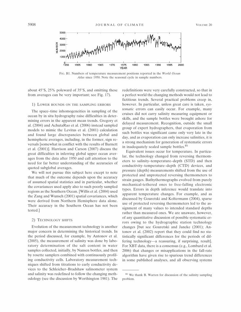
The number of values available each month in theWorld Ocean Atlas is shown in Fig. B1. Note, amongother issues, a visually prominent annual cycle in thenumber of samples. A well-known electrical engineer-ing result is that periodic sampling of a periodic signal(the annual cycle) can produce complex rectified sig-nals (e.g., Wozencraft and Jacobs 1965). A full discus-sion of the adequacy of error estimation in any of theavailable global climatologies is a major undertaking,depending as it does upon evaluating the interpolationand extrapolation rules used by the various authors tofill the very large data gaps. That very little data, altim-etry included, exists in the Southern Ocean is a particu-lar concern in all published subglobal averages.

A full discussion of the sampling problem is an elabo-rate exercise, largely because the a priori variance oftemperature and salinity measurements is a very strongfunction of both horizontal position and depth. If theocean were statistically homogeneous, failure to samplesignificant regions would have minor influence on com-putation of the mean. As it is, the general lack of datain the Southern Ocean until very recently is of especialconcern because it may well be behaving differentlythan the rest of the World Ocean (for context, about18% of both the ocean area and volume lie poleward of


about 45°S, 25% poleward of 35°S, and omitting thesefrom averages can be very important; see Fig. 17).

1) LOWER BOUNDS ON THE SAMPLING ERRORS

The space–time inhomogeneities in sampling of theocean by in situ hydrography raise difficulties in deter-mining errors in the apparent mean trends. Gregory etal. (2004) and AchutaRao et al. (2006) instead sampledmodels to mimic the Levitus et al. (2001) calculationand found large discrepancies between global andhemispheric averages, including, in the former, sign re-versals [somewhat in conflict with the results of Barnettet al. (2001)]. Harrison and Carson (2007) discuss thegreat difficulties in inferring global upper ocean aver-ages from the data after 1950 and call attention to theneed for far better understanding of the accuracies ofquoted subglobal averages.

We will not pursue this subject here except to notethat much of the outcome depends upon the accuracyof assumed spatial statistics and in particular, whetherthe covariances used apply also to such poorly sampledregions as the Southern Ocean. [Willis et al. (2004) usedthe Zang and Wunsch (2001) spatial covariances, whichwere derived from Northern Hemisphere data alone.Their accuracy in the Southern Ocean has not beentested.]

2) TECHNOLOGY SHIFTS

Evolution of the measurement technology is anothermajor concern in determining the historical trends. Inthe period discussed, for example, by Antonov et al.(2005), the measurement of salinity was done by labo-ratory determination of the salt content in watersamples collected, initially, by Nansen bottles, and thenby rosette samplers combined with continuously profil-ing conductivity cells. Laboratory measurement tech-niques shifted from titrations to early conductivity de-vices to the Schleicher–Bradshaw salinometer systemand salinity was redefined to follow the changing meth-odology (see the discussion by Worthington 1981). The

redefinitions were very carefully constructed, so that ina perfect world the changing methods would not lead tofictitious trends. Several practical problems creep in,however. In particular, unless great care is taken, sys-tematic errors can easily occur. For example, manycruises did not carry salinity measuring equipment orskills, and the sample bottles were brought ashore fordelayed measurement. Recognition, outside the smallgroup of expert hydrographers, that evaporation fromsuch bottles was significant came only very late in theday, and as evaporation can only increase salinities, it isa strong mechanism for generation of systematic errorsin inadequately sealed sample bottles.B1

Equivalent issues occur for temperature. In particu-lar, the technology changed from reversing thermom-eters to salinity–temperature–depth (STD) and thenconductivity–temperature–depth (CTD) devices, andpressure (depth) measurements shifted from the use ofprotected and unprotected reversing thermometers tostrain gauges. Bathythermographs evolved from purelymechanical-tethered ones to free-falling electronictypes. Errors in depth inference would translate intoapparent temperature changes. For example, and asdiscussed by Gouretski and Koltermann (2004), sparseuse of protected reversing thermometers led to the as-signment of many values to intended standard depthsrather than measured ones. We are unaware, however,of any quantitative discussion of possible systematic er-rors owing to the hydrographic station technologychanges [but see Gouretski and Jancke (2001); An-tonov et al. (2002) report that they could find no sta-tistically significant differences for the periods of dif-fering technology—a reassuring, if surprising, result].For XBT data, there is a consensus (e.g., Lombard et al.2006) that changes or misapplications in the fall-ratealgorithm have given rise to spurious trend differencesin some published analyses, and all observing systems

B1 We thank B. Warren for discussion of the salinity samplingproblem.

FIG. B1. Numbers of temperature measurement positions reported in the World OceanAtlas since 1950. Note the seasonal cycle in sample numbers.


inevitably are susceptible to systematic errors at somelevel (see also Gouretski and Koltermann 2007).

c. Forcing imbalances and surface boundaryconditions

One approach, in principle, to estimating sea levelrise would be to calculate it from the net heating andnet estimated evaporation minus precipitation minusrunoff (E � E � P � R) from the atmospheric reanaly-ses. The initial estimate for the boundary forcing of theECCO-GODAE model is taken from the NCEP–NCAR “reanalysis” of Kalnay et al. (1996), and windstress, freshwater, and enthalpy fluxes are part of thesystem control vector, and thus subject to adjustment torender the model consistent with the data. In the case ofthe meteorological forcing, the prior weights are an es-timate of the degree to which the atmospheric variablesare likely to be in error and thus expected to change.This atmospheric reanalysis poses several problems.

The Kalnay et al. (1996) estimate and its subsequentupgrades were computed from a weather forecastmodel and data assimilation method. No global con-straints were applied, and thus considerable imbalancesin the global water and heat budgets are present. Forexample, in one NCEP–NCAR release, the net esti-mated � to the ocean was found to average 6 cm ofwater yr�1, and the net heating of the ocean exceeded2 W m�2 (see P. Heimbach and C. King 2006, unpub-lished manuscript). Béranger et al. (2006) found differ-ences extending over more than 10° of latitude exceed-ing 1 m yr�1 in various published zonal precipitationclimatologies. Global imbalances have no known nega-tive influence on weather forecasting skill and so haveattracted little attention. For our purposes, they couldbe disastrous.

Considerable controversy exists surrounding the netinput of freshwater to the ocean, involving as it doesdetermining the net loss of continental and sea iceas well as runoff and water storage (e.g., Rignot andThomas 2002; Cazenave 2006). Because of the debateover the sign of net ice volume changes, and the way inwhich weights are changed in the calculations to guidethe minimization, it is very difficult to rigorously assignan a priori net input of freshwater. Effectively, over the13 yr, the prior estimate is zero with an error estimateof �0.16 mm yr�1. It is estimated a priori that the glo-bal heating by the atmosphere is 1 W m�2 (e.g., Barnettet al. 2001; Hansen et al. 2005, from coupled models)with an unknown uncertainty, but estimated by us ini-tially as �0.6 W m�2 [inferred from Hansen et al.(2005), but clearly very crude]. Note that 1 W m�2 heat-ing corresponds to a sea level rise of approximately 1.3mm yr�1.

Achieving balanced freshwater fluxes is a critical pre-requisite when forcing the model with freshwaterboundary conditions, rather than the unphysical virtualsalt flux boundary conditions (Huang 1993), as well asavoiding restoring sea surface salinity, which mighthave further spurious effects. P. Heimbach and C. King(2006, unpublished manuscript) summarize freshwaterimbalances in the NCEP–NCAR I reanalysis. They findthat none of ocean-only E � P, or E � P � R, or trulyglobal E � P are balanced. The ECCO-GODAE stateestimates, which used virtual salt flux boundary condi-tions through version 2.199, were able to reduce theimbalance somewhat, but not to a degree sufficient toavoid severe distortions to the signal in sea surface el-evation.

The estimation framework permits addressing defi-ciencies in the E � P fluxes. We require the global(over ocean) E to approximately vanish over the 13-yrperiod via a suitable extra term in the misfit function.The gradient of the misfit with respect to E provides thenecessary adjustments needed, while ensuring that themodel minus observation misfits are not degraded. Thisterm has been applied starting with the use of freshwa-ter flux boundary conditions in v2.200. In addition, aglobal mean and trend in E has been removed in v2.200as a first guess to speed up the convergence.

APPENDIX C

Model Issues

The MITgcm, in its existing ECCO-GODAE con-figuration, like most ocean models, employs the Bouss-inesq approximation. Net heating or cooling of a Bouss-inesq model affects the spatial-mean bottom pressure,but leaves the spatial-mean sea surface unchanged. Incontrast, adding or subtracting freshwater affects boththe mean sea surface elevation and the mean bottompressure. Here, following Greatbatch (1994), the spa-tial-mean bottom pressure change owing to changes inmean density is converted into an equivalent spatial-mean sea level rise. It is important to note, however(see Dewar 1998; McDougall et al. 2002; Huang and Jin2002; Losch et al. 2004), that other approximations areburied in the Boussinesq numerics and their influenceon regional and global sea level change is obscure.

Another important set of approximations involvesthe way in which the free surface import and export offreshwater takes place across the model sea surface, aproblem that Huang (1993) and others have called at-tention to. We can identify at least six different surfaceboundary conditions for freshwater and salt in use ingeneral circulation models (P. Heimbach and J.-M.


Campin 2006, unpublished manuscript; see Table 2). Inregions of sea ice formation and melting, approxima-tions are made to the exchange of salt between ice andocean, and with the way in which the mass of floatingice is represented in bottom pressures. See, for ex-ample, Campin et al. (2004) and Griffies (2004) for fur-ther discussion of model approximations at the sea sur-face. Here, we rely primarily on the system involving alinear free surface and virtual salt flux (number 2 inTable 2) because it produces consistent estimates of thefreshwater exchange, which is not true, for example, forsystem 3.

Many other approximations, including the renderingof continuous partial differential equations as discrete,the parameterizations of eddy flux terms, neglect ofseafloor heating, truncated equations of state, etc. un-derlie all model calculations. The extent to which theyproduce systematic effects that generate spurious tem-poral trends in model volume or mass totals is notknown, and thus any results from long model integra-tions should be viewed with caution.

REFERENCES

AchutaRao, K. M., B. D. Santer, P. J. Gleckler, K. E. Taylor,D. W. Pierce, T. P. Barnett, and T. M. L. Wigley, 2006: Vari-ability of ocean heat uptake: Reconciling observations andmodels. J. Geophys. Res., 111, C05019, doi:10.1029/2005JC003136.

Adcroft, A., J. R. Scott, and J. Marotzke, 2001: Impact of geo-thermal heating on the global ocean circulation. Geophys.Res. Lett., 28, 1735–1738.

Antonov, J. I., S. Levitus, and T. P. Boyer, 2002: Steric level varia-tions during 1957–1994: Importance of salinity. J. Geophys.Res., 107, 8013, doi:10.1029/2001JC000964.

——, ——, and ——, 2005: Thermosteric sea level rise, 1955–2003.Geophys. Res. Lett., 32, L12602, doi:10.1029/2005GL023112.

Barnett, T. P., D. W. Pierce, and R. Schnur, 2001: Detection ofanthropogenic climate change in the world’s oceans. Science,292, 270–274.

Béranger, K., B. Barnier, S. Gulev, and M. Crépon, 2006: Com-paring 20 years of precipitation estimates from differentsources over the World Ocean. Ocean Dyn., 56, 104–138.

Campin, J.-M., A. Adcroft, C. Hill, and J. Marshall, 2004: Con-servation of properties in a free-surface model. Ocean Mod-ell., 6, 221–244.

Carton, J. A., B. S. Geise, and S. A. Grodsky, 2005: Sea level riseand the warming of the oceans in the Simple Ocean DataAssimilation (SODA) ocean reanalysis. J. Geophys. Res.,110, C09006, doi:10.1029/2004JC002817.

Cazenave, A., 2006: How fast are the ice sheets melting? Science,314, 1250–1252.

——, and R. S. Nerem, 2004: Present-day sea level change: Ob-servations and causes. Rev. Geophys., 42, RG3001,doi:10.1029/2003RG000139.

Chelton, D. B., J. C. Ries, B. J. Haines, L. L. Fu, and P. S. Calla-han, 2001: Satellite altimetry. Satellite Altimetry and EarthSciences: A Handbook of Techniques and Applications, L.-L.Fu and A. Cazenave, Eds., Academic Press, 1–131.

Church, J., J. M. Gregory, P. Huybrechts, M. Kuhn, K. Lambeck,M. T. Nhuan, D. Qin, and P. L. Woodworth, 2001: Changes insea level. Climate Change 2001: The Scientific Basis, J. T.Houghton et al., Eds., Cambridge University Press, 639–693.

Curry, R., and C. Mauritzen, 2005: Dilution of the northern NorthAtlantic Ocean in recent decades. Science, 308, 1772–1774.

Dewar, W. K., 1998: Calculation of pressure in ocean simulations.J. Phys. Oceanogr., 28, 577–588.

Douglas, B. C., M. S. Kearney, and S. R. Leatherman, Eds., 2001:Sea Level Rise: History and Consequences. Academic Press,232 pp.

Fekete, B. M., C. J. Vörösmarty, and W. Grabs, 2002: High-resolution fields of global runoff combining observed riverdischarge and simulated water balances. Global Biogeochem.Cycles, 16, 1042, doi:10.1029/1999GB001254.

Fernandes, M. J., S. Barbosa, and C. Lázaro, 2006: Impact of al-timeter data processing on sea level studies. Sensors, 6, 131–163.

Forget, G., and C. Wunsch, 2007: Estimated global hydrographicvariability. J. Phys. Oceanogr., 37, 1997–2008.

Fu, L.-L., and A. Cazenave, Eds., 2001: Satellite Altimetry andEarth Sciences: A Handbook of Techniques and Applications.Academic Press, 463 pp.

Gille, S. T., 2002: Warming of the Southern Ocean since the 1950s.Science, 295, 1275–1277.

——, 2004: How nonlinearities in the equation of state of seawatercan confound estimates of steric sea level change. J. Geophys.Res., 109, C03005, doi:10.1029/2003JC002012.

Gould, J., and Coauthors, 2004: Argo profiling floats bring newera of in situ ocean observations. Eos, Trans. Amer. Geophys.Union, 85, 170, 190–191.

Gouretski, V. V., and K. Jancke, 2001: Systematic errors as thecause for an apparent deep water property variability: Globalanalysis of the WOCE and historical hydrographic data.Prog. Oceanogr., 48, 337–402.

——, and K. P. Koltermann, 2004: WOCE global hydrographicclimatology: A technical report. Berichte des Bundesamtesfür Seeschifffahrt und Hydrographie 35, 52 pp. and two CD-ROMs.

——, and ——, 2007: How much is the ocean really warming?Geophys. Res. Lett., 34, L01610, doi:10.1029/2006GL027834.

Greatbatch, R. J., 1994: A note on the representation of steric sealevel in models that conserve volume rather than mass. J.Geophys. Res., 99, 12 767–12 771.

Gregory, J. M., H. T. Banks, P. A. Stott, J. A. Lowe, and M. D.Palmer, 2004: Simulated and observed decadal variabilityin ocean heat content. Geophys. Res. Lett., 31, L15312,doi:10.1029/2004GL020258.

Griffies, S. M., 2004: Fundamentals of Ocean Climate Models.Princeton University Press, 518 pp.

Hansen, J., and Coauthors, 2005: Earth’s energy imbalance: Con-firmation and implications. Science, 308, 1431–1435.

Harrison, D. E., and M. Carson, 2007: Is the World Ocean warm-ing? Upper-ocean temperature trends: 1950–2000. J. Phys.Oceanogr., 37, 174–187.

Huang, R. X., 1993: Real freshwater flux as a natural boundarycondition for the salinity balance and thermohaline circula-tion forced by evaporation and precipitation. J. Phys. Ocean-ogr., 23, 2428–2446.

——, and X. Jin, 2002: Sea surface elevation and bottom pressureanomalies due to thermohaline forcing. Part I: Isolated per-turbations. J. Phys. Oceanogr., 32, 2131–2150.


Ishii, M., M. Kimoto, K. Sakamoto, and S.-I. Iwasaki, 2006: Stericsea level changes estimated from historical ocean subsurfacetemperature and salinity analyses. J. Oceanogr., 62, 155–170.

Jackett, D. R., and T. J. McDougall, 1995: Minimal adjustment ofhydrographic profiles to achieve static stability. J. Atmos.Oceanic Technol., 12, 381–389.

Jenkins, G. M., and D. G. Watts, 1968: Spectral Analysis and ItsApplications. Holden-Day, 525 pp.

Kalnay, E., and Coauthors, 1996: The NCEP/NCAR 40-Year Re-analysis Project. Bull. Amer. Meteor. Soc., 77, 437–471.

Köhl, A., D. Stammer, and B. Cornuelle, 2007: Interannual todecadal changes in the ECCO global synthesis. J. Phys.Oceanogr., 37, 313–337.

Lavallée, D. A., T. van Dam, G. Blewitt, and P. J. Clarke, 2006:Geocenter motions from GPS: A unified observation model.J. Geophys. Res., 111, B05405, doi:10.1029/2005JB003784.

Leuliette, E. W., R. S. Nerem, and G. T. Mitchum, 2004: Resultsof TOPEX/Poseidon and Jason-1 calibration to construct acontinuous record of mean sea level. Mar. Geod., 27, 79–94.

Levitus, S., J. I. Antonov, J. Wang, T. L. Delworth, K. W. Dixon,and A. J. Broccoli, 2001: Anthropogenic warming of Earth’sclimate system. Science, 292, 267–270.

Lombard, A., A. Cazenave, P.-Y. LeTraon, S. Guinehut, and C.Cabanes, 2006: Perspectives on present-day sea level change:A tribute to Christian le Provost. Ocean Dyn., 56, 445–451.

Losch, M., A. Adcroft, and J.-M. Campin, 2004: How sensitive arecoarse general circulation models to fundamental approxima-tions in the equations of motion? J. Phys. Oceanogr., 34,306–319.

Lyman, J. M., J. K. Willis, and G. C. Johnson, 2006: Recent cool-ing of the upper ocean. Geophys. Res. Lett., 33, L18604,doi:10.1029/2006GL027033.

Marshall, J., A. Adcroft, C. Hill, L. Perelman, and C. Helsey,1997: A finite-volume, incompressible Navier–Stokes modelfor studies of the ocean on parallel computers. J. Geophys.Res., 102, 5753–5766.

McDougall, T. J., R. J. Greatbatch, and Y. Y. Lu, 2002: On con-servation equations in oceanography: How accurate areBoussinesq ocean models? J. Phys. Oceanogr., 32, 1574–1584.

Miller, L., and B. C. Douglas, 2004: Mass and volume contribu-tions to twentieth-century global sea level rise. Nature, 428,406–409.

Mitchum, G. T., 1998: Monitoring the stability of satellite altim-eters with tide gauges. J. Atmos. Oceanic Technol., 15, 721–730.

Mitrovica, J. X., M. E. Tamisiea, J. L. Davis, and G. A. Milne,2001: Recent mass balance of polar ice sheets inferred frompatterns of global sea-level change. Nature, 409, 1026–1029.

——, J. Wahr, I. Matsuyama, A. Paulson, and M. E. Tamisiea,2006: Reanalysis of ancient eclipse, astronomic and geodeticdata: A possible route to resolving the enigma of global sea-level rise. Earth Planet Sci. Lett., 243, 390–399.

Munk, W., 2002: Twentieth century sea level: An enigma. Proc.Natl. Acad. Sci. USA, 99, 6550–6555.

——, 2003: Ocean freshening, sea level rising. Science, 300, 2041–2043.

Nerem, R. S., 1995: Global mean sea level variations fromTOPEX/POSEIDON altimeter data. Science, 268, 708–710.

——, 1997: Global mean sea level change: Correction. Science,275, 1053.

Patullo, J. G., W. H. Munk, R. Revelle, and E. Strong, 1955: Theseasonal oscillation in sea level. J. Mar. Res., 14, 88–155.

Peltier, W. R., 2001: Global glacial isostatic adjustment and mod-ern instrumental records of relative sea level history. SeaLevel Rise: History and Consequences, B. C. Douglas, M. S.Kearney, and S. P. Leatherman, Eds., Academic Press, 65–95.

Pierce, D. W., T. P. Barnett, K. M. Achutarao, P. J. Gleckler,J. M. Gregory, and W. M. Washington, 2006: Anthropogenicwarming of the oceans: Observations and model results. J.Climate, 19, 1873–1900.

Plag, H.-P., 2006: Recent relative sea-level trends: An attempt toquantify the forcing factors. Philos. Trans. Roy. Soc. London,A364, 821–844.

Ponte, R., C. Wunsch, and D. Stammer, 2007: Spatial mapping oftime-variable errors in Jason-1 and TOPEX/Poseidon seasurface height measurements. J. Atmos. Oceanic Technol., 24,1078–1085.

Rignot, E., and R. H. Thomas, 2002: Mass balance of polar icesheets. Science, 297, 1502–1506.

Stammer, D., 1997: Steric and wind-induced changes in TOPEX/POSEIDON large-scale sea surface topography observa-tions. J. Geophys. Res., 102, 20 987–21 010.

——, A. Köhl, and C. Wunsch, 2007: Impact of accurate geoidfields on estimates of the ocean circulation. J. Atmos. OceanicTechnol., 24, 1464–1478.

Wenzel, M., and J. Schröter, 2007: The global ocean mass budgetin 1993–2003 estimated from sea level change. J. Phys.Oceanogr., 37, 203–213.

Willis, J. K., D. Roemmich, and B. Cornuelle, 2004: Interannualvariability in upper ocean heat content, temperature, andthermosteric expansion on global scales. J. Geophys. Res.,109, C12036, doi:10.1029/2003JC002260.

——, J. M. Lyman, G. C. Johnson, and J. Gilson, 2007: Correctionto “Recent cooling of the upper ocean.” Geophys. Res. Lett.,34, L16601, doi:10.1029/2007GL030323.

Woodworth, P., J. M. Gregory, and R. J. Nicholls, 2004: Longterm sea level changes and their impacts. The Sea, A. R.Robinson and K. Brink, Eds., Biological-Physical Interac-tions in the Sea, Vol. 12, Harvard University Press, 717–752.

Worthington, L. V., 1981: The water masses of the world ocean:Some results of a fine-scale census. Evolution of PhysicalOceanography, B. A. Warren and C. Wunsch, Eds., MITPress, 42–69.

Wozencraft, J. M., and I. M. Jacobs, 1965: Principles of Commu-nication Engineering. Wiley, 720 pp.

Wunsch, C., 2006: Discrete Inverse and State Estimation Problems:With Geophysical Fluid Applications. Cambridge UniversityPress, 371 pp.

——, and P. Heimbach, 2007: Practical global oceanic state esti-mation. Physica D, 230, 197–208.

Zang, X., and C. Wunsch, 2001: Spectral description of low-frequency oceanic variability. J. Phys. Oceanogr., 31, 3073–3095.


Decadal Trends in Sea Level Patterns: 1993–2004ocean.mit.edu/~cwunsch/papersonline/Wunschetal_jclimate...Decadal Trends in Sea Level Patterns: 1993–2004 CARL WUNSCH Department

Documents