THE JOURNAL OF FINANCE • VOL. LX, NO. 3 • JUNE 2005 Debt Dynamics CHRISTOPHER A. HENNESSY and TONI M. WHITED ∗ ABSTRACT We develop a dynamic trade-off model with endogenous choice of leverage, distri- butions, and real investment in the presence of a graduated corporate income tax, individual taxes on interest and corporate distributions, financial distress costs, and equity flotation costs. We explain several empirical findings inconsistent with the static trade-off theory. We show there is no target leverage ratio, firms can be savers or heavily levered, leverage is path dependent, leverage is decreasing in lagged liq- uidity, and leverage varies negatively with an external finance weighted average Q. Using estimates of structural parameters, we find that simulated model moments match data moments. THE MILLER (1977) PERPETUAL TAX SHIELD FORMULA has served as one of the major references for those evaluating whether taxes can explain observed financing patterns. This formula is a cornerstone of the static trade-off theory, which posits that firms weigh the tax benefits of debt against costs associated with fi- nancial distress and bankruptcy. This benchmark model has provided intuition and guidance for much of the empirical literature on corporate capital struc- ture, which has uncovered several patterns in the data that are inconsistent with the static trade-off theory. For example, Graham (2000) finds that, “Paradoxically, large, liquid, prof- itable firms with low expected distress costs use debt conservatively.” By debt “conservatism,” Graham means that firms fail to issue sufficient debt to drive their expected marginal corporate tax rate down to that consistent with a zero/low net benefit to debt based on the Miller formula. In yet another blow to the theory, Myers (1993) states, “The most telling evidence against the static trade-off theory is the strong inverse correlation between profitability and fi- nancial leverage ... Higher profits mean more dollars for debt service and more taxable income to shield. They should mean higher target debt ratios.” Baker and Wurgler (2002) reject the trade-off theory on different grounds, stating, “The trade-off theory predicts that temporary f luctuations in the market to book ratio or any other variable should have temporary effects.” Based on finding ∗ Hennessy is from the University of California at Berkeley. Whited is from the University of Wisconsin, Madison. We would like to thank an anonymous referee, Rob Stambaugh, Alan Auerbach, Joao Gomes, Gilles Chemla, Tom George, Terry Hendershott, Dirk Jenter, Malcolm Baker, Murray Frank, Sheridan Titman, and Jonathan Willis for detailed comments. We also thank seminar participants at the Federal Reserve Board, MIT, the University of British Columbia, and the University of Houston. 1129

Welcome message from author
This document is posted to help you gain knowledge. Please leave a comment to let me know what you think about it! Share it to your friends and learn new things together.
Transcript

THE JOURNAL OF FINANCE • VOL. LX, NO. 3 • JUNE 2005
Debt Dynamics
CHRISTOPHER A. HENNESSY and TONI M. WHITED∗
ABSTRACT
We develop a dynamic trade-off model with endogenous choice of leverage, distri-butions, and real investment in the presence of a graduated corporate income tax,individual taxes on interest and corporate distributions, financial distress costs, andequity flotation costs. We explain several empirical findings inconsistent with thestatic trade-off theory. We show there is no target leverage ratio, firms can be saversor heavily levered, leverage is path dependent, leverage is decreasing in lagged liq-uidity, and leverage varies negatively with an external finance weighted average Q.Using estimates of structural parameters, we find that simulated model momentsmatch data moments.
THE MILLER (1977) PERPETUAL TAX SHIELD FORMULA has served as one of the majorreferences for those evaluating whether taxes can explain observed financingpatterns. This formula is a cornerstone of the static trade-off theory, whichposits that firms weigh the tax benefits of debt against costs associated with fi-nancial distress and bankruptcy. This benchmark model has provided intuitionand guidance for much of the empirical literature on corporate capital struc-ture, which has uncovered several patterns in the data that are inconsistentwith the static trade-off theory.
For example, Graham (2000) finds that, “Paradoxically, large, liquid, prof-itable firms with low expected distress costs use debt conservatively.” By debt“conservatism,” Graham means that firms fail to issue sufficient debt to drivetheir expected marginal corporate tax rate down to that consistent with azero/low net benefit to debt based on the Miller formula. In yet another blow tothe theory, Myers (1993) states, “The most telling evidence against the statictrade-off theory is the strong inverse correlation between profitability and fi-nancial leverage . . . Higher profits mean more dollars for debt service and moretaxable income to shield. They should mean higher target debt ratios.” Bakerand Wurgler (2002) reject the trade-off theory on different grounds, stating,“The trade-off theory predicts that temporary fluctuations in the market to bookratio or any other variable should have temporary effects.” Based on finding
∗Hennessy is from the University of California at Berkeley. Whited is from the Universityof Wisconsin, Madison. We would like to thank an anonymous referee, Rob Stambaugh, AlanAuerbach, Joao Gomes, Gilles Chemla, Tom George, Terry Hendershott, Dirk Jenter, MalcolmBaker, Murray Frank, Sheridan Titman, and Jonathan Willis for detailed comments. We also thankseminar participants at the Federal Reserve Board, MIT, the University of British Columbia, andthe University of Houston.
1129
1130 The Journal of Finance
a negative relationship between leverage and an “external finance weightedaverage market to book ratio,” they conclude that “capital structure is the cu-mulative outcome of attempts to time the equity market.”
This paper shows that a dynamic trade-off model can explain these styl-ized facts. As such, it provides a convincing alternative to the hypotheses ofnonmaximizing behavior, Myers’ (1984) pecking order theory, and/or markettiming. Our results also reconcile the puzzles cited above with the evidencepresented by MacKie-Mason (1990) and Graham (1996a) that taxes matter. Weoffer a sensible interpretation of the difference between our conclusions andthose in much of the rest of the literature: The latter has taken a static modeland compared its predictions with data generated by firms making a sequenceof dynamic financing decisions. However, corporations do not face an infiniterepetition of the Miller (1977) financing problem. Consequently, his frameworkis an inappropriate basis for assessing whether a rational tax-based model canexplain observed leverage ratios.
Accordingly, we address the seeming anomalies by solving and simulatinga dynamic model of investment and financing under uncertainty, where thefirm faces a realistic tax environment, small equity flotation costs, and fi-nancial distress costs. The firm maximizes its value by making two interre-lated decisions: How much to invest and whether to finance this investmentinternally, with debt, or with external equity. The firm can either borrow orsave and can be in one of three equity regimes (positive distributions, zerodistributions, or equity issuance.) The firm is forward-looking, making cur-rent investment and financing decisions in anticipation of future financingneeds.
The logic of our argument is as follows. Traditional formulations of the fi-nancing decision place the firm at “date zero” with no cash on hand. Such firmsare at the debt versus external equity financing margin, since each dollar ofdebt replaces a dollar of external equity. The problem with the traditional ap-proach is that corporations do not spend their lives at date zero. Rather, theyevolve in a stochastic way, finding themselves at different financing marginsover time.
As an illustration, consider a firm that realized a high profit shock last pe-riod, with internal cash exceeding desired investment. Rather than choosingbetween debt and external equity, this firm must choose between retentionand distribution of the excess funds. Note also that each dollar of debt issuedby this high liquidity firm would serve to increase the distribution to share-holders, rather than replacing external equity. As intuition would suggest, ourmodel shows that the marginal increase in debt (reduction in savings) is moreattractive when it serves as a replacement for external equity and is less attrac-tive when it finances an increase in distributions to shareholders. Since highliquidity firms are more likely to be at the latter financing margin, they issueless debt.
This example illustrates the pitfalls associated with the traditional staticframework. The more general message to take away is that, given the impor-tance of a corporation’s endogenous financing margin, characterization of how
Debt Dynamics 1131
the tax system influences the financial and investment policies of a rationalfirm necessitates a forward-looking dynamic framework.
We highlight the main empirical implications. First, absent any invocationof market timing or adverse selection premia, the model generates a negativerelationship between leverage and lagged measures of liquidity, consistent withthe evidence in Titman and Wessels (1988), Rajan and Zingales (1995), andFama and French (2002). Second, even though the model features single-perioddebt, leverage exhibits hysteresis, in that firms with high lagged debt use moredebt than otherwise identical firms. This is because firms with high lagged debtare more likely to find themselves at the debt versus external equity margin.Third, since lagged leverage is a function of the firm’s history, financial policyis path dependent. Finally, the combination of path dependence and hysteresisis sufficient to generate a data series containing the main Baker and Wurgler(2002) results in a rational model without market timing or adverse selectionpremia.
The model is sufficiently parsimonious that it can be taken directly to data.Because of the discrete nature of the tax environment, it is impossible to gen-erate smooth, closed-form estimating equations from the model. Therefore,we turn to simulation methods, employing the indirect inference technique inGourieroux, Monfort, and Renault (1993) and Gourieroux and Monfort (1996).Specifically, we solve the model via value function iteration and then use thissolution to generate a simulated panel of firms. Our indirect inference proce-dure picks parameter estimates by minimizing the distance between interestingmoments from actual data and the corresponding moments from the simulateddata. This procedure has an important advantage over traditional regressions:It does not suffer from simultaneity problems, since it requires none of the zero-correlation restrictions that are necessary to identify OLS and IV regressions.Rather, as in a standard GMM estimation, it merely requires at least as manymoments as underlying structural parameters.
Our model is most similar to those developed by Gomes (2001) and Cooleyand Quadrini (2001). The key differences between our model and that of Gomesare that we include taxation, model debt issuance explicitly, and allow the cor-poration to save. We place greater emphasis on financing since we seek to ex-plain empirical leverage relationships, whereas Gomes focuses upon invest-ment. Cooley and Quadrini (2001) examine industry dynamics in a model thatexplicitly treats the choice between debt and equity in a setting without taxes.Firms rent rather than purchase physical capital, and their model imposes acap on the equity of the firm and, hence, liquid assets. This cap is rationalized byassuming the corporation earns a lower rate of return on financial investmentsthan shareholders.
In related papers, Fischer, Heinkel, and Zechner (FHZ) (1989) and Goldstein,Ju, and Leland (GJL) (2001) formulate dynamic trade-off models with exoge-nous investment and distribution policies. Brennan and Schwartz (1984) andTitman and Tsyplakov (2003) endogenize investment, but maintain the as-sumption that free cash is distributed to shareholders. Of critical importancein understanding the contribution of our paper is that all four models hold
1132 The Journal of Finance
the gross tax advantage of debt constant, independent of whether the firm isfinancially constrained or unconstrained.
In a recent empirical paper, Leary and Roberts (2004a) find that a modifiedversion of the FHZ model, featuring fixed plus convex adjustment costs, canexplain many of the stylized facts regarding financial timing and can also bereconciled with the empirical findings of Baker and Wurgler (2002). Strebulaev(2004) formulates a dynamic trade-off model with adjustment costs similar tothat of GJL. Simulations of his model, and indirectly of the GJL model, produceresults broadly consistent with the empirical evidence in Baker and Wurgler(2002).1
Although variants of the FHZ and GJL models enjoy some empirical support,Leary and Roberts (2004a, 2004b) present evidence directly supportive of ourdynamic trade-off model and inconsistent with that of FHZ and GJL. In par-ticular, they find that the gap between internal funds and anticipated capitalexpenditures is a key determinant of financial policy. Firms issue debt—andto a lesser extent equity—when the financing gap is large. The firm’s financ-ing gap plays no role in the FHZ and GJL models, although it is of centralimportance in our formulation. Consistent with our model, Leary and Roberts(2004a) also find that higher profitability is associated with significantly lessexternal financing: Equity and debt. However, the FHZ and GJL models predictthat firms respond to profitability shocks by going into the capital markets andissuing more debt.
The findings in Leary and Roberts (2004a) and Strebulaev (2004) may temptsome to conclude that adjustment costs are necessary to reconcile the trade-offtheory with the empirical evidence.2 Our results show that this is not true.Since our firm dynamically optimizes over leverage, payouts, and investmenteach and every period, it is always at a “restructuring point” and still generatesa data series consistent with the stylized facts.
Our paper is also related to the public finance literature assessing the effectof the dividend tax, with Auerbach (2000) providing a recent survey. Sinn (1991)presents a deterministic model in which the firm cannot issue debt, and mustchoose between internal and external equity. Auerbach (2000) presents a moresatisfactory treatment of the effect of taxation on financial policy. However, hismodel: (1) is deterministic; (2) has no investment decision; (3) has no cost ofequity issuance; (4) assumes a flat rate corporate income tax; and (5) imposesexogenous dividend and repurchase constraints.3
Another contribution of our model is that it determines optimal financialslack. Kim, Mauer, and Sherman (1998) bound corporate saving by setting anexogenous lower rate of return on corporate financial investments. Almeida,Campello, and Weisbach (2004) remove the precautionary motive for saving
1 See also an ambitious paper by Schurhoff (2004), who formulates a trade-off theoretic modelwith realization-based capital gains taxes.
2 The respective authors do not claim that such costs are necessary. Rather, their contention isthat adding adjustment costs to the trade-off theory is sufficient to explain the findings in Bakerand Wurgler (2002).
3 In fairness, Auerbach intends to present a simple model contrasting alternative theories.
Debt Dynamics 1133
by imposing a finite horizon. Shyam-Sunder and Myers (1999) foreshadow ourapproach, arguing that “tax or other costs of holding excess funds” may compeldistributions. However, their discussion begs the following questions. First,exactly what are the “tax costs” associated with slack? Second, since peckingorder theory assumes “taxes are second order,” then at what point do taxesbecome first order? Finally, what is the optimal amount of slack and how doesit vary with tax rates and costs of external funds? Our model answers eachquestion explicitly.
Before proceeding, it should be noted that 40 years ago Modigliani and Miller(1963, p. 442) articulated the need for precisely the type of model developed inthis paper, stating:
The existence of a tax advantage for debt financing . . . does not necessar-ily mean that corporations should at all times seek to use the maximumpossible amount of debt . . . For one thing, other forms of financing, notablyretained earnings, may in some circumstances be cheaper still when thetax status of investors under the personal income tax is taken into ac-count. More important, there are, as we pointed out, limitations imposedby lenders . . . which are not fully comprehended within the frameworkof static equilibrium models, either our own or those of the traditionalvariety.
The details of the dynamic model that Modigliani and Miller seemed to havein mind have never been worked out. Consequently, empiricists have been leftwith little formal guidance in interpreting the signs and magnitudes of the re-gression coefficients implied by the theory. Bridging the divide between theoryand data is the objective of this paper.
The remainder of the paper is organized as follows. Section I provides severalsimple examples that explain the main intuitive results. Section II presentsthe model, and Sections III and IV derive the optimal financial and investmentpolicies, respectively. Section V shows that under reasonable parameter values,the model generates regression coefficients consistent with the stylized facts.Section VI describes our data and the indirect inference procedure. Section VIIconcludes.
I. The Basic Argument
The following stylized examples convey the central intuition of the dynamicmodel. For the purpose of simplicity, this section fixes the firm’s real investmentpolicy; ignores uncertainty; and assumes constant tax rates on corporate in-come, individual interest income, and corporate distributions, denoted by τc, τi,and τd, respectively. These assumptions are relaxed in the model presented inSection II.
Let r be the rate of return on the taxable riskless Treasury bill. Now, considerthe standard “date zero” firm with no internal cash evaluating the choice be-tween debt and external equity. Assume the firm knows marginal funds will bedistributed next period. Reducing debt by one dollar increases next period’s
1134 The Journal of Finance
distribution by 1 + r(1 − τc), with the shareholder receiving the followingamount after distribution taxes:4
1 + r(1 − τc)(1 − τd ). (1)
Now assume that each dollar raised in the equity market costs the shareholder1 + λ, where λ is interpreted as flotation costs. Reducing debt by one dollarrequires the shareholder to give up 1 + λ in the current period. If the share-holder had been able to invest these funds on his own account, rather thancontributing them to the firm for the purpose of debt reduction, he would haveearned
(1 + λ)[1 + r(1 − τi)]. (2)
Therefore, it is better to leave the debt outstanding when
(1 + λ)[1 + r(1 − τi)] > 1 + r(1 − τc)(1 − τd ) (3)
⇒ λ[1 + r(1 − τi)]r
> τi − [τc + τd (1 − τc)]. (4)
If λ = 0, the above analysis yields the “traditional” condition on tax rates suchthat debt dominates external equity
τc >τi − τd
1 − τd. (5)
Note that Miller derives his condition for the optimality of debt finance (5) byimplicitly setting up a firm at the debt versus external equity margin with non-negative distributions to shareholders in all future periods (see Miller (1977),footnote 18). Following Graham (2000), we temporarily choose as base-caseparameters τi = 29.6% and τd = 12%. Under these tax rates, the traditionalcondition (5) implies that debt should be issued so long as τc > 20%.
Despite the common use of condition (5) as a gauge of debt conservatism, wewill show that it is only applicable if the firm has no internal funds in this periodand knows it will make positive distributions next period. Indeed, consider anotherwise identical firm, except that it has different expectations regardingnext period’s equity regime. In particular, assume that rather than making adistribution next period, the firm anticipates issuing equity. That is, externalequity represents next period’s marginal source of funds. If the firm retiresa unit of debt this period, required equity issuance next period is reduced by1 + r(1 − τc). Next period, this saves the shareholder
(1 + λ)[1 + r(1 − τc)]. (6)
Reducing debt by one dollar requires the shareholder to give up 1 + λ in thecurrent period. If the shareholder had been able to invest these funds on his
4 This expression adopts Stiglitz’s (1973) assumption that the dollar of equity injected into thefirm is treated as a “return of capital” exempt from the distribution tax.
Debt Dynamics 1135
own account, rather than contributing them to the firm for the purpose of debtreduction, he would have earned
(1 + λ)[1 + r(1 − τi)]. (7)
In this context, it is better to leave the debt outstanding if τc > τi. Conversely,when τc < τi, the optimal policy is to issue sufficient equity this period to retireall debt. This argument is not circular. We made no assumption regarding thesource of funds this period. The firm was free to choose between debt and equity.Rather, the assumption adopted was that the firm anticipates external equitybeing the marginal source of funds next period. In this setting, it is optimal todelay equity issuance when the shareholder can earn a higher after-tax rate ofreturn on savings than the corporation. Note also that under the assumed taxrates, the critical corporate tax rate needed to induce debt issuance is 29.6%,which is above the traditional trigger given in (5), which is equal to 20%. Inother words, the case for debt finance is weaker when the firm anticipatesissuing equity next period, rather than distributing.
The previous two examples illustrated how the choice between debt and ex-ternal equity depends upon the firm’s expected equity regime next period. Thenext example illustrates the importance of the firm’s current financial position.In contrast to a firm needing external funds, consider a firm like Microsoft, withinternal funds well in excess of the amount needed to fund the real investmentprogram. Rather than choosing between debt and external equity, such a firmmust choose between retention and distribution of excess funds.
Suppose the CFO anticipates that marginal funds will be distributed nextperiod. If the funds are distributed today, the shareholder receives (1 − τd). Byinvesting the funds on his own account, the shareholder receives the followingamount next period:
(1 − τd )[1 + r(1 − τi)]. (8)
In contrast, if the funds are retained for the purpose of corporate saving, theshareholder receives the following amount next period after distribution taxes:
(1 − τd )[1 + r(1 − τc)]. (9)
In this context, it is better to distribute and reduce internal savings, if τc > τi.The corporation will want to reduce savings as long as its tax rate exceeds29.6%, which differs from the traditional trigger for the dominance of debt overexternal equity, which is 20% under the assumed tax rates. Intuitively, theshareholder prefers the firm to distribute the funds if he can invest at a higherafter-tax rate of return than the corporation. Similar results are derived byKing (1974), Auerbach (1979), and Bradford (1981).
The above discussion focused on some extreme circumstances. In reality,firms can be in three possible equity regimes: Positive distributions, zero distri-butions, or negative distributions (equity issued). In addition, the equity regimenext period should be modeled as the outcome of an optimizing decision overfinancing and real investment policies in light of the realized state. The model
1136 The Journal of Finance
presented in the next section does so. Having said this, the simple examplesprovided above suggest the following insights. First, the optimal financial pol-icy and target marginal corporate tax rate depend upon the firm’s current eq-uity regime and expectations regarding next period’s equity regime. Second,optimal financial policy will exhibit path dependence, since the firm’s historydetermines its current financing margin.
II. The Model
A. Technology and Financing
Time is discrete and the horizon infinite. Operating profits (π ) depend uponcapital (k) and a shock (z). The space of capital inputs is denoted by K ⊆ �+,with the corresponding measurable space denoted by (K , K). Characteristics ofthe operating profit function and shock are described below.
ASSUMPTION 1: The operating profit function π : K × Z → �+ is twice continu-ously differentiable, strictly increasing, strictly concave, and satisfies the Inadaconditions:
limk↓0
π1(k, z) = ∞ ∀ z ∈ Z ,
limk↑∞
π1(k, z) = 0 ∀ z ∈ Z .
ASSUMPTION 2: The profit shock takes values in a compact set Z ≡ [z¯, z] with
Borel subsets Z. The transition function � on (Z , Z) is Markov, monotone, sat-isfies the Feller property, and has no atoms.5
Concavity of the operating profit function occurs under imperfect competition,where the firm faces a downward-sloping demand curve. Alternatively, Lucas(1978) argues that limited managerial or organizational resources result indecreasing returns. The variable z reflects shocks to demand, input prices, orproductivity.
The firm has four potential sources of funds: external equity, current cashflow, single-period debt, and internal savings. The model incorporates a pro-gressive corporate income tax, personal taxes on interest income, personal taxeson distributions to shareholders, costs of financial distress, a collateral con-straint, and equity flotation costs. The first four financial frictions representthe traditional ingredients of the trade-off theory, while the last two frictionsadd realism and tractability to the model. Equally important to note are thetheories excluded. In particular, there is no notion of adjustment costs, markettiming, or the rules of thumb implicit in the pecking order.
We now discuss each financial friction in detail. Smith (1977) provides de-tailed evidence on direct equity flotation costs. Using these data, Gomes (2001)
5 The “no atoms” condition is not necessary for Propositions 1–4, since the results also hold whenZ is a countable set.
Debt Dynamics 1137
estimates that the marginal flotation cost is 2.8%. To reflect such costs, weadopt the following assumption.
ASSUMPTION 3: For each dollar of external equity paid into the firm, there is aflotation cost λ > 0.
In Section V, we simulate the model assuming λ = 2.8%, seeing whether adynamic trade-off model with small flotation costs generates regression coeffi-cients broadly consistent with the stylized facts. In Section VI, indirect inferenceis used to estimate λ and other parameters of interest.
The static trade-off theory posits that corporations weigh tax advantages ofdebt against distress costs. In order to capture this trade-off, we assume thatfinancial distress necessitates a “fire sale” in which capital is sold at a depressedprice (s < 1) in order to make the promised debt payment.
ASSUMPTION 4: If end-of-period internal funds are insufficient to meet debt obli-gations, a fire sale occurs, with capital sold for s < 1. Outside of financial distress,the firm may buy and sell capital for a price of 1.
In support of Assumption 4, Asquith, Gertner, and Scharfstein (1994) docu-ment that asset sales are a common response to distress. The existence of firesale costs is documented in two studies by Pulvino (1998, 1999), who findsthat constrained and distressed airlines receive lower prices on the sale of air-craft than healthy airlines. In addition, as emphasized in Duffie and Singleton(1999), distress is often a correlated event. In the event of correlated distress,it may be necessary to reallocate capital across sectors. In a study of aerospaceplant closings, Ramey and Shapiro (2001) find that reallocated capital sells ata discount.
The next assumption introduces a collateral constraint.
ASSUMPTION 5: The firm may borrow and lend at the risk-free rate r before taxes.The lender imposes a collateral constraint requiring that the fire sale value ofcapital be sufficient to pay the loan.
Assumption 5 is made for two reasons. First, an extensive theoretical andempirical literature suggests that firms face collateral constraints (see, e.g.,Stiglitz and Weiss (1981), Bernanke and Gertler (1989), Whited (1992), Kiyotakiand Moore (1997), and Clementi and Hopenhayn (2002)). Second, Assumption 5greatly simplifies the numerical problem solved below, eliminating the need tosolve for the promised yield to maturity that would be requested by the lenderwhen the value of liquidated assets is insufficient to cover the promised debtpayment.
The endogenous state variable p′ represents the face value of debt, withpayment coming due next period. Positive (negative) values of p′ imply thefirm is borrowing (lending). The feasible set for p′ is denoted by P ⊆ �, withthe corresponding measurable space denoted by (P , P).
1138 The Journal of Finance
Limiting the firm to single-period debt precludes simultaneous borrowingand lending. When debt is single-period, increasing borrowing and lending inequal amounts constitutes a “neutral permutation” of the optimal policy, withinterest income canceling interest expense. A natural extension of the modelwould be to derive optimal maturity structure, allowing the firm to borrow atlong maturities while lending/borrowing at short maturities.6 Such a modelmight rationalize the observed tendency of firms to simultaneously borrow andlend. Alternative explanations for simultaneous borrowing and lending by cor-porations include transactional demand for cash, sinking-fund provisions inbond covenants, and banks requiring compensating deposits.
B. Taxation
Investors are homogeneous and risk neutral. The tax rate on interest is τi, im-plying investors use r(1 − τi) as their discount rate. Following Bradford (1981),we assume shareholders are taxed at rate τd on corporate distributions. Themodel does not impose any constraint on dividends or share repurchases. Noris any assumption made regarding whether the corporation uses dividends orshare repurchases as the method for disgorging funds. Rather, we follow Brad-ford in assuming there is a flat rate of tax applied to the total amount dis-tributed. This approach allows us to characterize optimal distribution policy,as opposed to optimal dividend policy. In particular, our model pins down thetotal amount paid to shareholders, not the means of distribution. As such, themodel is silent on the “dividend puzzle.”
In the context of the current U.S. income tax system, theory suggests thatcorporations should use share repurchases as the main vehicle for disgorgingcash if the marginal shareholder is a taxable individual.7 There are three ad-vantages of share repurchases. First, capital gains historically have enjoyed alower statutory tax rate than dividends. Second, shareholder basis is excludedfrom tax, creating a tax deferral advantage. Finally, there is a tax-free stepup inbasis at death. In a detailed study, Green and Hollifield (2003) find that underan optimal repurchasing strategy, the effective tax rate on capital gains is only60% of the statutory rate.8
Corporate taxable income (y) is equal to operating profits less economic de-preciation (which occurs at rate δ) less interest expense, plus interest income
y(k, p, z) ≡ π (k, z) − δk − r(
p1 + r
). (10)
The corporate tax function is denoted by g, with the marginal corporate tax rate(τc) satisfying
6 This extension is related to the models of optimal debt maturity in Leland and Toft (1996) andLeland (1998).
7 Corporate shareholders may prefer dividends to repurchases due to dividend exclusion rules.8 However, Feldstein and Summers (1979) show that the failure to index basis for inflation can
create effective capital gains tax rates over 100%.
Debt Dynamics 1139
τc[ y(k, p, z)] ≡ g1[ y(k, p, z)]. (11)
Assumptions regarding the tax system are summarized below.
ASSUMPTION 6: Investors are taxed at flat rates of τi ∈ (0, 1) on interest in-come and τd ∈ (0, 1) on corporate distributions. The corporate tax functiong : Y → � is twice differentiable, strictly increasing, strictly convex, and satisfiesg(0) = 0
limy→∞ τc( y) ≡ τc < 1;
limy→−∞ τc( y) = 0;
τc > τi.
In reality, firms with negative taxable income do not receive a check from theU.S. Treasury. Rather, losses may be carried back 2 years and carried forward20 years. The convex tax schedule g is intended to capture the effects of theloss limitation provisions in a tractable way. For a careful treatment of the losslimitation rules and the implications for effective marginal tax rates, the readeris referred to Graham (1996a, 1996b).
The condition τc > τi is imposed for tractability, although it is not necessary.As is shown below, the condition τc > τi is necessary to generate bounded savingsand induce distributions of excess liquidity. If the condition is not met, themodel yields the prediction that the optimal policy for a corporation with excessliquidity is to save everything. We revisit this condition in Section III wherethe optimal financial policy is characterized.
The collateral constraint requires that the sum of after-tax cash flow plusthe liquidation value of capital is at least as large as the promised debtpayment
p′ ≤ s ∗ k′(1 − δ) + π (k′, z¯) − g ( y(k′, p′, z
¯)). (12)
If realized after-tax cash flow is insufficient to cover debt service, the firmsells the minimum amount of capital needed to make the promised payment.The random variable n denotes the number of units of capital sold in a firesale
n(k′, p′, z ′) ≡ max{
0,p′ − [π (k′, z ′) − g ( y(k′, p′, z ′))]
s
}. (13)
Since π − g has positive support, savers never conduct fire sales.The firm chooses k′ at the start of the period, with the actual end of period
capital stock, after fire sales, being stochastic. The variable i(k, p, k′, z) denotesthe funds required to change the capital stock to k′, given the current state (k,p, z)
i(k, p, k′, z) ≡ k′ − [k(1 − δ) − n(k, p, z)]. (14)

1140 The Journal of Finance
C. The Firm’s Problem
Each period, the vector (k, p, z) summarizes the state, with the firm choosingoptimal investment and financial policies. Without loss of generality, attentioncan be confined to compact K. As in Gomes (2001), define k as follows:
π (k, z) − δk ≡ 0. (15)
Under Assumption 1, k is well defined. Since k > k is not economically prof-itable, let
K ≡ [0, k]. (16)
The debt limit based on the collateral constraint (12) is increasing and concavein k′ and is denoted by p(k′). Since k′ is chosen from a compact set K, it followsthat p is bounded above. In order to ensure compactness of the set P, it isconvenient to assume there is an arbitrarily low bound on p′, denoted by p
¯.
This lower bound is imposed without loss of generality, since Assumption 6ensures bounded saving. From this analysis, it follows that the choice set K × Pis nonempty, compact, and convex.
Each period, cash flow to shareholders before distribution taxes or flotationcosts is equal to
max{π (k, z) − g ( y(k, p, z)) − p, 0} + p′
1 + r− i(k, p, k′, z). (17)
The first term in brackets in (17) is operating profits less corporate taxes lessdebt payments. When this term is negative, the lender collects all after-taxearnings, leaving equity with zero. The last two terms represent cash inflow(outflow) from new borrowing (lending) and the investment cost, respectively.
Let �s and �n be indicators for states in which fire sales do and do not occur,respectively. Substituting (13) and (14) into (17) and rearranging terms, thecash flow to shareholders, before flotation costs and distribution taxes, may beexpressed as
π (k, z) − g ( y(k, p, z)) − p�n + s�s
− [k′ − k(1 − δ)] + p′
1 + r. (18)
From (18), it can be seen that the economic effect of fire sales is to increase thereal cost per dollar of debt service in distressed states.
Letting �d, �i, and �0 be indicators for positive distributions, equity issuance,and zero distributions, respectively, the net cash flow to shareholders is
e(k, p, k′, p′, z) ≡ [1 + �iλ − �dτd ]
×[π (k, z) − g ( y(k, p, z)) − p
�n + s�s− [k′ − k(1 − δ)] + p′
1 + r
]. (19)
The function e is continuous and strictly concave in its first two arguments.Fire sales, distribution taxes, and flotation costs generate kinks that cause thefunction e to be nondifferentiable for states (k, p, z), such that either
Debt Dynamics 1141
π (k, z) − g ( y(k, p, z)) = p, (20)
ore(k, p, k′, p′, z) = 0. (21)
The objective of the manager is to maximize the discounted value of net cashflow to shareholders
Vt0 = Et0
{ ∞∑t=t0
(1
1 + r(1 − τi)
)(t−t0)
et
}. (22)
The Bellman equation for this problem is
V (k, p, z) = max(k′, p′)∈K ×P
e(k, p, k′, p′, z)
+[
11 + r(1 − τi)
] ∫V (k′, p′, z ′)�(z, dz′). (23)
The following propositions, proved in the Appendix, characterize the value func-tion and optimal policy correspondence (h).
PROPOSITION 1: There is a unique continuous function V : K × P × Z → �+ sat-isfying (23).
PROPOSITION 2: For each z ∈ Z, the equity value function V(·, ·, z) : K × P → �+is strictly increasing (decreasing) in its first (second) argument and strictlyconcave.
PROPOSITION 3: The optimal policy correspondence h(·, ·, z) : K × P → K × P is acontinuous single-valued function.
PROPOSITION 4: At each (k, p, z) in the interior of K × P × Z, such that
π (k, z) − g ( y(k, p, z)) �= p,
e(k, p, k′, p′, z) �= 0,(24)
the equity value function V(·, ·, z) is continuously differentiable in its first twoarguments with derivatives given by
Vi(k, p, z) = ei(k, p, k′, p′, z) for i = 1, 2.
III. Optimal Financial Policy
This section derives the optimal financial policy holding fixed the investmentprogram, with the next deriving the optimal investment rule in light of thefirm’s financial policy.
A. The Marginal Costs and Benefits of Debt
The budget constraint (19) may be restated as
1142 The Journal of Finance
p′
1 + r− e(k, p, k′, p′, z)
1 + �iλ − �dτd= i(k, p, k′, z) − max{π (k, z) − g ( y(k, p, z)) − p, 0}
= k′ − k(1 − δ) − π (k, z) − g ( y(k, p, z)) − p�n + s�s
. (25)
The left side of (25) represents sources of external funds and the right side rep-resents the financing gap, which is the excess of investment costs over internalfunds. Constrained (Unconstrained) firms have positive (negative) financinggaps.
We derive the optimal financial policy holding fixed the financing gap. To doso, consider a firm at an arbitrary state (k, p, z) evaluating a candidate financingpolicy p′ satisfying e(k, p, k′, p′, z) �= 0. Consider a perturbation increasing p′
with the funds used to finance an increase in e. Since the right side of (25)is being held fixed, the implicit function theorem implies that along the “iso-funding” line
(∂e∂p′
)∣∣∣∣isofund
= 1 + �iλ − �dτd
1 + r. (26)
Assuming differentiability of the value function, the total change in the rightside of (23) resulting from a small increase in p′ is
�(k, p, k′, p′, z) = 1 + �iλ − �dτd
1 + r
+[
11 + r(1 − τi)
] ∫V2(k′, p′, z ′)�(z, dz′). (27)
Proposition 4 implies that so long as (24) holds, the value function is differen-tiable, with
V2(k′, p′, z ′) = −[1 + �′iλ − �′
dτd ][
1 + r[1 − τc( y(k′, p′, z ′))](1 + r)(�′
n + s�′s)
]. (28)
The “no atoms” condition in Assumption 2 implies that (20) occurs on a set ofmeasure zero, so that this kink point can be disregarded in deriving the optimalpolicies.
Finally, we must pin down V2 for states such that e = 0. It is shown below thatthe end-of-period equity regime hinges upon p′. High savings make it probablethat positive distributions occur, while high debt is associated with equity is-suance. Intermediate values of p′ are associated with zero distributions (e = 0).Having established concavity of the value function in Proposition 2, it followsthat when e = 0, V2 must be somewhere between the extremes implied by (28).Therefore, we denote the derivative of the value function in zero distributionstates as
Debt Dynamics 1143
V2(k′, p′, z ′) ≡ −[1 + φ(k′, p′, z ′)][
1 + r[1 − τc( y(k′, p′, z ′))](1 + r)(�′
n + s�′s)
]
φ(k′, p′, z ′) ∈ (−τd , λ).(29)
Substituting (28) and (29) into (27) and multiplying by (1 + r) yields an ex-pression for the net marginal benefit from increasing debt (reducing saving)
(1 + r) ∗ �(k, p, k′, p′, z) = MB(k, p, k′, p′, z) − MC(k′, p′, z) (30)
MB(k, p, k′, p′, z) ≡ 1 + �iλ − �dτd (31)
MC(k′, p′, z) ≡∫
[1 + �′iλ − �′
dτd + �′0φ
′][1 + r(1 − τc( y(k′, p′, z ′)))][1 + r(1 − τi)](�′
n + s�′s)
�(z, dz′).
(32)
The term MB represents the marginal benefit to shareholders from increas-ing debt, reflecting either increased distributions or lower equity contributions.The term MC represents the expected discounted marginal cost of servicing thedebt.
The current state (k, p, z) is fixed and the financial perturbation treats k′ as aconstant. Therefore, the only argument in the MB function being changed is p′.As p′ is increased, the MB schedule steps down from 1 + λ to 1 − τd at a uniqueswitch-point, denoted by p′
0 where
e[k, p, k′, p′0, z] ≡ 0. (33)
From (25), it follows that p′0/(1 + r) is just equal to the firm’s financing gap
p′0(k, p, k′, z)
1 + r≡ i(k, p, k′, z) − max{π (k, z) − g ( y(k, p, z)) − p, 0}
= k′ − k(1 − δ) − π (k, z) − g ( y(k, p, z)) − p�n + s�s
.
(34)
From (25), it follows that the sign of p′0 depends on firm status, with
Unconstrained ⇒ p′0(k, p, k′, z) < 0
Constrained ⇒ p′0(k, p, k′, z) > 0.
When evaluating whether to increase debt, shareholders compare themarginal benefit with the marginal cost, with the latter represented by theMC schedule. The direct cost to the corporation of debt service is 1 + r(1 − τ ′
c),and this term appears in the numerator of (32). The term 1 + r(1 − τi) in thedenominator is the discount rate. The MC schedule contains two other termsaffecting the shadow cost of debt service. The term �′
n + s�′s in the denomina-
tor implies that the economic cost of debt service is high when there is a high
1144 The Journal of Finance
probability of a fire sale. Finally, the term 1 + �′iλ − �′
dτd + �′0φ
′ reflects thefact that debt service is most (least) costly for a firm that expects to be issuing eq-uity (making a distribution) at the margin next period. The effect of decreasingsaving is analogous.
From (32), it follows that the marginal cost of debt service is increasing inthe amount of debt issued
∂MC(k′, p′, z)∂p′ > 0. (35)
The reasoning is as follows. First, increasing p′ reduces taxable income (y′) inevery state (z′). Therefore, the expected marginal corporate tax rate is decreas-ing in the amount of debt issued. Symmetrically, the expected after-tax returnon corporate saving declines in the amount saved, discouraging precautionarysaving. Second, raising p′ increases the likelihood of a fire sale (�′
s = 1). Finally,it is shown below that raising p′ increases the likelihood of resorting to positiveequity issuance next period (�′
i = 1).In characterizing the optimal financial policy, it will also be useful to note the
limiting behavior of the MC schedule. Because of the fact that τc > τi, firms witharbitrarily high savings will make a distribution at the margin next period. Inaddition, such firms converge to the maximum corporate tax rate. Therefore,9
limp′↓−∞
MC(k′, p′, z) = (1 − τd )[1 + r(1 − τc)]1 + r(1 − τi)
< 1 − τd . (36)
B. Graphical Exposition
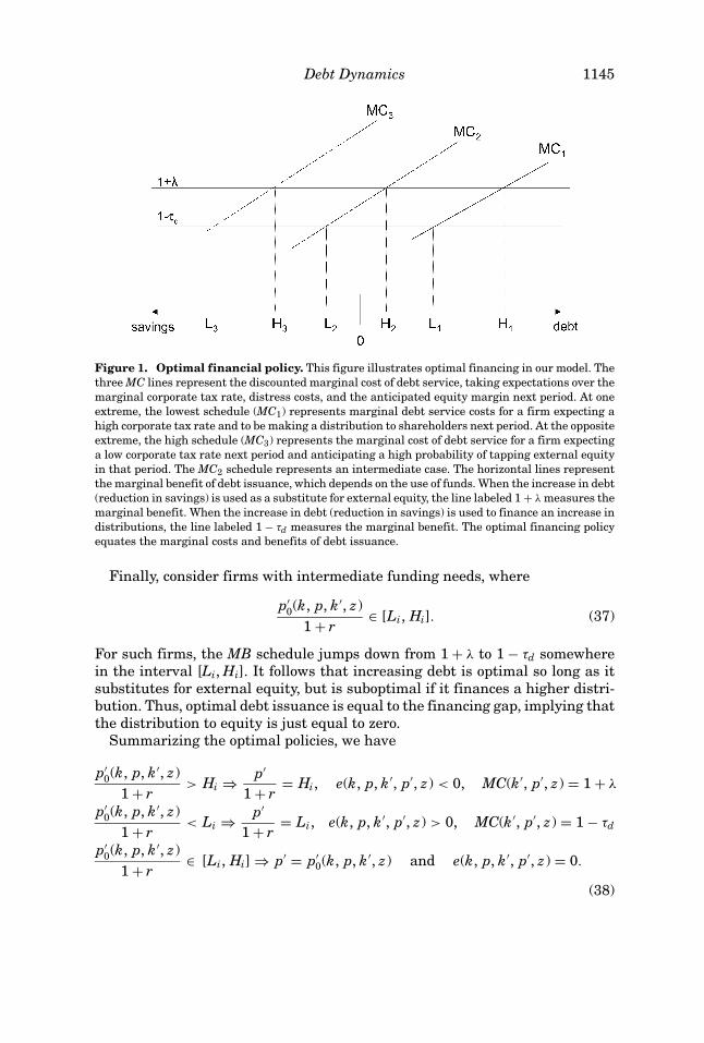
Figure 1 depicts the optimal financial policy for three potential MC sched-ules. The decision-making process is similar for each schedule. To see this, as-sume the firm faces one of the three MCi schedules. Now, consider a firm withp′
0/(1 + r) > Hi. For this firm, the marginal benefit from increasing leverageis 1 + λ for debt levels less than or equal to Hi. Starting from the far left, themarginal benefit of reducing saving or increasing debt exceeds the marginalcost until Hi is reached. Increasing debt beyond Hi is suboptimal. Since thefirm chooses p′ < p′
0, it follows that equity issuance covers the remaining fi-nancing gap (e < 0).
Now consider a less constrained firm facing the same schedule MCi, withp′
0/(1 + r) < Li. The optimal debt issuance is equal to Li < Hi. This firm issuesless debt than the more constrained firm, because the marginal dollar of debtgoes toward a distribution rather than replacing costly external equity. Therelevant marginal benefit schedule is 1 − τd, which exceeds the marginal costto the left of Li, but is less than the marginal cost for higher debt levels. Sincedebt issuance exceeds the financing gap, it follows that a positive distribution(e > 0) is made.
9 If, contrary to Assumption 6, τc ≤ τi , then the unconstrained corporation never makes adistribution.
Debt Dynamics 1145
Figure 1. Optimal financial policy. This figure illustrates optimal financing in our model. Thethree MC lines represent the discounted marginal cost of debt service, taking expectations over themarginal corporate tax rate, distress costs, and the anticipated equity margin next period. At oneextreme, the lowest schedule (MC1) represents marginal debt service costs for a firm expecting ahigh corporate tax rate and to be making a distribution to shareholders next period. At the oppositeextreme, the high schedule (MC3) represents the marginal cost of debt service for a firm expectinga low corporate tax rate next period and anticipating a high probability of tapping external equityin that period. The MC2 schedule represents an intermediate case. The horizontal lines representthe marginal benefit of debt issuance, which depends on the use of funds. When the increase in debt(reduction in savings) is used as a substitute for external equity, the line labeled 1 + λ measures themarginal benefit. When the increase in debt (reduction in savings) is used to finance an increase indistributions, the line labeled 1 − τd measures the marginal benefit. The optimal financing policyequates the marginal costs and benefits of debt issuance.
Finally, consider firms with intermediate funding needs, where
p′0(k, p, k′, z)
1 + r∈ [Li, Hi]. (37)
For such firms, the MB schedule jumps down from 1 + λ to 1 − τd somewherein the interval [Li, Hi]. It follows that increasing debt is optimal so long as itsubstitutes for external equity, but is suboptimal if it finances a higher distri-bution. Thus, optimal debt issuance is equal to the financing gap, implying thatthe distribution to equity is just equal to zero.
Summarizing the optimal policies, we have
p′0(k, p, k′, z)
1 + r> Hi ⇒ p′
1 + r= Hi, e(k, p, k′, p′, z) < 0, MC(k′, p′, z) = 1 + λ
p′0(k, p, k′, z)
1 + r< Li ⇒ p′
1 + r= Li, e(k, p, k′, p′, z) > 0, MC(k′, p′, z) = 1 − τd
p′0(k, p, k′, z)
1 + r∈ [Li, Hi] ⇒ p′ = p′
0(k, p, k′, z) and e(k, p, k′, p′, z) = 0.
(38)
1146 The Journal of Finance
This indicates that there is no target leverage ratio. Firms can be borrowers orsavers under the optimal program, depending on the financing gap and positionof the MC schedule.
We now turn to the optimal policies under each of the three specific MC sce-narios depicted in Figure 1. Consider first the firm facing the low MC1 schedule,where
MC(k′, 0, z) < 1 − τd . (39)
Referring to (32), the condition (39) is most likely to hold when the probabilityof making a positive distribution next period (�′
d = 1) is high. In addition, it iseasily verified that a necessary condition for (39) is∫
τc[ y(k′, 0, z ′)]�(z, dz′) > τi. (40)
The low MC1 scenario is most likely to hold for cash cow corporations thatexpect to be in the top tax bracket, such as UST in the Mitchell (2000) casestudy. Under the low MC1 scenario, firms are heavily levered. In fact, evenunconstrained firms are willing to issue debt (L1) in order to finance higherdistributions. Such behavior is a clear violation of the static pecking order.
Moving to the opposite extreme, consider the optimal financial policy whenthe firm faces the MC3 schedule, where
MC(k′, 0, z) > 1 + λ. (41)
From (32), it follows that in order for (41) to be satisfied, the probability ofbeing in the equity issuance regime next period must be high. In addition, anecessary condition for (41) is∫
τc[ y(k′, 0, z ′)]�(z, dz′) < τi. (42)
The high MC3 scenario is most likely to hold for high growth firms with lowtaxable income. Under the high MC3 scenario, firms avoid debt completely,with the tax disadvantage to debt at the personal level swamping the benefit ofdeducting interest expense at the corporate level. Firms with p′
0/(1 + r) > H3exhibit a striking departure from the static pecking order. These firms simul-taneously save and issue equity, despite the fact that riskless debt finance isavailable.
The last scenario to be considered features the intermediate MC2 schedule,satisfying
1 − τd < MC(k′, 0, z) < 1 + λ. (43)
From (32), it can be seen that this scenario is most likely to emerge when theprobability of being in either the positive distribution or equity issuance regimesis not too high. In this scenario, unconstrained firms do not issue debt and donot tap external equity. Those unconstrained firms with p′
0/(1 + r) < L2 make
Debt Dynamics 1147
positive distributions to shareholders, while those with p′0/(1 + r) ∈ [L2, 0) set
the distribution to zero. Severely constrained firms, with p′0/(1 + r) > H2, utilize
a mixture of debt and external equity, with equity being the marginal sourceof funds. Constrained firms with p′
0/(1 + r) ∈ (0, H1) use debt as their marginalsource of funds, issuing no equity and making no distributions to shareholders.
Finally, it is interesting to note that the firm facing intermediate marginalcosts of debt service follows a financial policy strikingly similar to that predictedby Myers’ (1984) pecking order theory. This potential observational equivalenceshould be kept in mind in empirical tests pitting the dynamic trade-off theoryagainst the pecking order.
C. Empirical Implications
Despite the fact that debt is single-period in our model, leverage is predictedto exhibit hysteresis. To see this, consider two firms with the same capital stock(k) and shock (z), with one of the firms having higher lagged debt. For a givenchoice of k′, the two firms face the same MC(k′, ·, z) schedule. It follows from(25) that the firm with higher lagged debt has a larger financing gap, with(38) indicating that debt issuance is weakly increasing in the financing gap.The hysteresis effect is due to the fact that, ceteris paribus, higher lagged debt(p) causes the firm to occupy the high portion of the marginal benefit sched-ule (1 + λ) over a longer stretch. That is, with higher lagged debt, more debtmust be issued this period before the marginal unit of debt serves to increasedistributions rather than replacing external equity.
The theory offers a potential explanation for the debt conservatism of highliquidity firms, documented by Graham (2000). For high liquidity firms likeMicrosoft, debt issuance serves to finance higher distributions to shareholders,rather than replacing costly external equity. Since high liquidity firms occupythe lower portion of the MB schedule, debt issuance is less attractive.
It is harder to predict the implications of the model for standard OLS regres-sions treating leverage as the dependent variable. Positive shocks (z) result inhigher lagged cash flow (π − g − p), which lowers the financing gap. Ceterisparibus, this results in lower leverage. However, positive shocks also raise thedesired capital stock, (k′), which increases the financing gap. To the extent thataverage Q picks up the latter effect, one would predict the coefficient on laggedmeasures of profitability to be negative. Given this ambiguity, in Section V,we simulate the model under reasonable parameter values, pinning down theimplied regression coefficients.
D. The Target Corporate Tax Rate
Using the Miller (1977) tax shield formula, Graham (2000) integrates un-der “net of personal tax benefit curves” to determine the target corporate taxrate. In a dynamic setting, the traditional target marginal corporate tax rate ismost likely incorrect. The expected marginal corporate tax rate under the opti-mal dynamic policy is a complicated function of the current equity regime and
1148 The Journal of Finance
expectations regarding next period’s equity regime. Proposition 5 illustratesthis point
PROPOSITION 5: If the collateral constraint does not bind, then:
e(k, p, k′, p′, z) < 0
⇒∫
[1 + �′iλ − �′
dτd + �′0φ
′][1 + r(1 − τc( y(k′, p′, z ′)))][1 + r(1 − τi)](�′
n + s�′s)
�(z, dz′) = 1 + λ.
e(k, p, k′, p′, z) > 0
⇒∫
[1 + �′iλ − �′
dτd + �′0φ
′][1 + r(1 − τc( y(k′, p′, z ′)))][1 + r(1 − τi)](�′
n + s�′s)
�(z, dz′) = 1 − τd .
e(k, p, k′, p′, z) = 0 ⇒ 1 − τd
<
∫[1 + �′
iλ − �′dτd + �′
0φ′][1 + r(1 − τc( y(k′, p′, z ′)))]
[1 + r(1 − τi)](�′n + s�′
s)�(z, dz′) < 1 + λ.
Clearly, the traditional ratio in (5) is a faulty basis for gauging debt con-servatism or poor tax planning on the part of corporations. To take a concreteexample, return to the tax rate assumptions in Section I and consider the CFOof a company like Microsoft. This company is unconstrained, has negative lever-age, and is making distributions at the margin each period. Suppose also thatthe corporation finds itself with an expected corporate tax rate equal to 25%given its current plan. Application of the target tax rate formula in (5) suggeststhat the corporation should make a larger distribution, reducing the amountsaved, and driving down the expected marginal tax rate to 20%.
In contrast, our model suggests that the firm in this example should actuallyreduce its distribution and increase savings. Intuitively, under the current plan,the firm earns a higher after-tax return than shareholders, who face a personaltax rate of 29.6% on interest income. Shareholders would therefore prefer re-tention of funds. To see this more formally, we may use the second optimalitycondition in Proposition 5 and set �′
n = �′d = 1. In this case, the target expected
marginal corporate tax rate is 29.6%, not 20%.
IV. Optimal Real Investment Policy
Consider the firm in an arbitrary state (k, p, z) evaluating an investment plank′ satisfying e(k, p, k′, p′, z) �= 0. To pin down the optimal real investment policy,we evaluate the effect on the maximand of a small increase in k′ to be financedin accordance with the optimal financial policy. Assuming differentiability ofthe value function, the change in the maximand is
de(k, p, k′, p′, z)dk′ +
(1
1 + r(1 − τi)
)
×∫ [
V1(k′, p′, z ′) +(
∂p′
∂k′
)V2(k′, p′, z ′)
]�(z, dz′). (44)
Debt Dynamics 1149
The first term in (44) represents the direct cost of investment to the shareholderin terms of the current distribution. The first term in the expectation is simplythe discounted value of a unit of installed capital, with the second representingthe costs associated with servicing incremental debt used to finance the project.From the firm’s budget constraint, the investment funding condition may bestated as
dedk′ = −[1 + �iλ − �dτd ]
[1 −
(1
1 + r
) (∂ p′
∂k′
)]. (45)
From Proposition 5, we know that when the optimal financial policy entailsnonzero distributions (e �= 0):
− [1 + �iλ − �dτd ][1 + r(1 − τi)]1 + r
=∫
V2(k′, p′, z ′)�(z, dz′). (46)
Substituting (45) and (46) into (44), the incremental gain from increasing thecapital stock is ∫ (
V1(k′, p′, z ′)1 + r(1 − τi)
)�(z, dz′) − [1 + �iλ − �dτd ]. (47)
The first term in (47) represents the expected discounted value of the marginalunit of installed capital, with the second representing the marginal cost ofinvestment, which takes into account the firm’s financing margin.
The envelope condition from Proposition 4 implies that for states in whichthe distribution to equity is nonzero
V1(k′, p′, z ′) = [1 + �′iλ − �′
dτd ][π1(k′, z ′)(1 − τ ′
c) + δτ ′c
�′n + s�′
s+ (1 − δ)
]. (48)
Having established concavity of the value function in Proposition 2, it followsthat when e′ = 0, then V1 lies somewhere between the extremes implied by (48).We denote the derivative of the value function in zero distribution states as
V1(k′, p′, z ′) ≡ [1 + φ(k′, p′, z ′)][π1(k′, z ′)(1 − τ ′
c) + δτ ′c
�′n + s�′
s+ (1 − δ)
]
φ′ ∈ (−τd , λ).
(49)
Substituting (48) and (49) into (47) yields, the following optimality condition
1 + �iλ − �dτd =∫ [
1 + �′iλ − �′
dτd + �′0φ
′
1 + r(1 − τi)
]
×[π1(k′, z ′)(1 − τ ′
c) + δτ ′c
�′n + s�′
s+ (1 − δ)
]�(z, dz′). (50)
The term on the left represents the direct cash cost to equity from increasinginvestment, with the right representing the shadow value of installed capital.Note that the cost to equity exhibits a downward jump at some level of capital
1150 The Journal of Finance
investment, call it k′0, at which the distribution to equity switches from negative
to positive. Some firms would then find themselves at a corner solution forcapital investment, finding it profitable to increase the capital stock up to k′
0,yet unwilling to incur the costs of external equity.
When the optimal policy entails nonzero distributions to equity, the invest-ment rule satisfies10
1 =∫ [
1 + �′iλ − �′
dτd + �′0φ
′
1 + �iλ − �dτd
]
×[
π1(k′, z ′)(1 − τ ′c) + δτ ′
c
[1 + r(1 − τi)][�′n + s�′
s]+ 1 − δ
1 + r(1 − τi)
]�(z, dz′). (51)
The first bracketed term reflects the potential for shifts in equity regimes acrossperiods. Ceteris paribus, investment incentives are stronger when the firm iscurrently in the positive distribution equity regime as opposed to the equityissuance regime. Intuitively, the incentive to invest is stronger when the fundsused for investment have a low opportunity cost. For a firm that is currentlymaking a distribution, the opportunity cost of retaining a marginal dollar isonly 1 − τd. In contrast, the opportunity cost of a dollar of external equity is1 + λ.
V. Simulation
Our empirical strategy proceeds as follows. First, we present a simulation ofthe model based on reasonable parameter values that we glean from previousstudies. Our intent is to ascertain whether our theory, with small equity flota-tion costs, can produce a cross section that embodies the anomalies we seekto explain. This exercise allows us to discriminate between our maximizingframework and other theories as vehicles for explaining observed phenomena.In Section VI, we use our data from COMPUSTAT to estimate the basic struc-tural parameters of the model. Since one of these parameters is λ, we will beable to estimate the magnitude of costs of external equity. Finally, we check thesensitivity of the model to variations in some of the key model parameters.
A. Design
In order to simulate our model, we need to choose a functional form for π :
π (k, z) = zkα, (52)
where α < 1 captures decreasing returns to scale. We assume the shock z followsan AR(1) process in logs:
ln(z ′) = ρ ln(z) + ε′, (53)
10 The optimality condition for the firm with a binding debt constraint contains an extra benefitterm attributable to the increase in p.
Debt Dynamics 1151
where ε′ ∼ N(0, σ 2ε ). We transform (53) into a discrete-state Markov chain us-
ing the method in Tauchen (1986), letting z have 20 points of support in[−3σε/
√1 − ρ2, 3σε/
√1 − ρ2].
The state space for (k, p, z) is discrete. The capital stock, k, lies in the set:[k, k(1 − δ)1/2, k(1 − δ), . . . , k(1 − δ)20],
where k is defined by (15). The state space for p is more complicated, becausedebt issuance is restricted by the collateral constraint (12), which in turn de-pends on the level of the capital stock. We specify the state space for p bychoosing feasible points in the candidate set that satisfy (12) for each elementof the state space for k. These state spaces for k and p appear to be sufficientfor our purposes in that the optimal policy never occurs at an endpoint of thestate space for k or at the lower endpoint of the state space for p.
Next we need to define the tax environment. For τd, we use the estimatein Graham (2000) of 0.12. We set the tax rate on interest income, τi, equal to0.25—a number slightly less than the Graham (2000) estimate of 0.296. Todefine the marginal corporate income tax schedule, we let N ( y , µτ , στ ) be thecumulative normal distribution function with mean µτ and standard deviationσ τ . The marginal tax rate function is
τc( y) = 0.35N ( y , µτ , στ );
the tax bill for positive y is given by∫ y
0τc(x) dx;
and the tax bill for negative y is given by
−∫ 0
yτc(x) dx.
For our first exercise, we parameterize our model along the lines of Gomes(2001) and Cooper and Ejarque (2001). From Gomes we take ρ = 0.62, σε =0.15, δ = 0.145, and λ = 0.028. Because Gomes uses a technological specifica-tion slightly different from ours, we turn to Cooper and Ejarque, who use anidentical production function, and we set α = 0.689. We set s equal to 0.75, anumber lying within the broad range of estimates of capital resale discounts inRamey and Shapiro (2001). Our two remaining parameters are (µτ , στ ), whichwe set so that the average realized marginal corporate tax rate is 0.30. Finally,we use a real risk-free interest rate of 0.025. As will be seen below, the stylizedfacts we generate with this simple simulation hold up when we base it on aparameterization obtained from our simulated moments estimation.
We solve the model via iteration on the Bellman equation, which produces thevalue function V(k, p, z) and the policy function {k′, p′} = h(k, p, z). Our modelsimulation proceeds by taking a random draw from the distribution of ε eachperiod, updating the z shock, and then computing V(k, p, z) and h(k, p, z). For
1152 The Journal of Finance
our initial exercise, we simulate the model for 10,000 time periods, droppingthe first 50 observations in order to allow the firm to work its way out of apossibly sub-optimal starting point.
Knowledge of h and V also allows us to compute interesting quantities suchas cash flow, Tobin’s Q, debt, and distributions. Specifically, we define our vari-ables to mimic the sorts of variables used in the literature.
Ratio of investment to the “book value” of assets (k′ − (1 − δ)k/kRatio of cash flow to the book value of assets (π (k, z) − g[y(k, p, z)] − p/k)Tobin’s Q (V(k, p, z) + p′/(1 + r))/k′Ratio of debt to the “market value” of assets (p′/(1 + r))/(V(k, p, z) + p′/(1 + r))Ratio of EBITDA to the book value of assets π (k, z)/kRatio of equity issuance to the book value of assets e(k, p, k′, p′, z)/k
Here, we have scaled all variables by the book value of assets, except for debt.We adopt this convention because of the use of market leverage in Rajan andZingales (1995) and Baker and Wurgler (2002).11
B. Results
Before presenting our simulation results, we examine the properties of thesimulated policy function, {k′, p′} = h(k, p, z). We start with the investment rule,where we note first that the choice of k′ depends on the current level of debt.If two firms with identical (k, z) come into the current period with differentstocks of outstanding debt, the one with higher debt never chooses a higher k′
and usually chooses a lower k′.The debt rule also exhibits several interesting characteristics. First, it is clear
that the choice of p′ not only depends on (k, z) but on the current level of p. Firmswith identical (k, z) and different p almost always choose different levels of p′.Further, the condition
∂p′
∂p≥ 0
always holds. As will be seen below, this hysteresis is important for generatingbehavior that appears to look like market timing. Second, large firms with lowprofit shocks tend to hold the most cash. This result is consistent with observed“debt conservatism.” Third, the debt rule displays substantial persistence: for afirm with a given (k, p) a large shock is required for an adjustment of debt policy.Finally, the firm engages in fire sales only if it has both a small capital stock anda large negative shock, and, in the simulations described and reported below, afire sale occurs at most 0.4% of the time. This result is particularly importantin that it suggests that our results are not driven by the collateral constraint.
11 It is worth noting that the results reported below change little when we normalize debt by thebook value of assets.
Debt Dynamics 1153
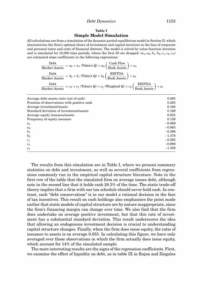
Table ISimple Model Simulation
All calculations are from a simulation of the dynamic partial-equilibrium model in Section II, whichcharacterizes the firm’s optimal choice of investment and capital structure in the face of corporateand personal taxes and costs of financial distress. The model is solved by value-function iterationand is simulated for 10,000 time periods, where the first 50 are dropped. (a1, a2, b1, b2, c1, c2, c3)are estimated slope coefficients in the following regressions:
DebtMarket Assets
= a0 + a1 (Tobin’s Q) + a2
(Cash Flow
Book Assets
)+ ua
DebtMarket Assets
= b0 + b1 (Tobin’s Q) + b2
(EBITDA
Book Assets
)+ ub
DebtMarket Assets
= c0 + c1 (Tobin’s Q) + c2 (Weighted Q) + c3
(EBITDA
Book Assets
)+ uc
Average debt-assets ratio (net of cash) 0.095Fraction of observations with positive cash 0.285Average investment/assets 0.160Standard deviation of investment/assets 0.169Average equity issuance/assets 0.055Frequency of equity issuance 0.139a1 −0.069a2 −0.865b1 −0.298b2 −1.378c1 −0.293c2 −0.908c3 −1.359
The results from this simulation are in Table I, where we present summarystatistics on debt and investment, as well as several coefficients from regres-sions commonly run in the empirical capital structure literature. Note in thefirst row of the table that the simulated firm on average issues debt, althoughnote in the second line that it holds cash 28.5% of the time. The static trade-offtheory implies that a firm with our tax schedule should never hold cash. In con-trast, such “debt conservatism” is in our model a rational decision in the faceof tax incentives. This result on cash holdings also emphasizes the point madeearlier that static models of capital structure are by nature inappropriate, sincethe firm’s financing margin can change over time. We also find that the firmdoes undertake on average positive investment, but that this rate of invest-ment has a substantial standard deviation. This result underscores the ideathat allowing an endogenous investment decision is crucial to understandingcapital structure changes. Finally, when the firm does issue equity, the ratio ofissuance to assets is on average 0.055. In calculating this figure, we have onlyaveraged over those observations in which the firm actually does issue equity,which account for 14% of the simulated sample.
The more interesting results are the signs of the regression coefficients. First,we examine the effect of liquidity on debt, as in table IX in Rajan and Zingales
1154 The Journal of Finance
(1995). Our first measure of liquidity, cash flow, comes in with a negative co-efficient in a regression of the debt to assets ratio on lagged Q and cash flow.Second, as seen in the next line of the table, this result is robust to our use ofEBITDA, as in Rajan and Zingales, as a measure of liquidity. The intuition forthese negative coefficients lies in the endogeneity of the firm’s equity regime. Inour model, firms that have experienced high profits have lower equity regimeswitch points (p′
0) and therefore tend to issue less debt. Finally, we run a re-gression similar to the one in equation (5) in Baker and Wurgler (2002), whereonce again the debt to assets ratio is the left side variable. The regressors arelagged Q, lagged EBITDA, and lagged external finance weighted Q. This lattervariable is constructed as in Baker and Wurgler (2002), where we use a 20 pe-riod moving average to calculate weighted Q.12 Note that we can replicate the“market timing” result in Baker–Wurgler with a time-invariant λ only equalto 0.028 to represent flotation costs. Our result is a product not of the cumu-lative attempts to time the equity market, but merely of debt hysteresis andthe fact that firms with large productivity shocks simultaneously have high Qsand tend to finance large desired investment with equity at the margin.
VI. Simulated Moments Parameter Estimation
Our data are from the full coverage 2002 Standard and Poor’s COMPUSTATindustrial files. We select a sample by first deleting firm–year observationswith missing data. Next, we delete observations in which total assets, the grosscapital stock, or sales are either zero or negative. To avoid rounding errors, wedelete firms whose total assets are less than two million dollars and gross capi-tal stocks are less than one million dollars. Further, we delete observations thatfail to obey standard accounting identities. Finally, we omit all firms whose pri-mary SIC classification is between 4,900 and 4,999 or between 6,000 and 6,999,since our model is inappropriate for regulated or financial firms. We end up withan unbalanced panel of firms from 1993 to 2001 with between 592 and 1128observations per year. We truncate our sample period below at 1993, becauseour tax parameters are relevant only for this period (see Graham (2000)).
Structural estimation of this model faces several challenges. First, the exis-tence of different equity regimes prevents the derivation of an Euler equationor decision rule that is a smooth function of the data. To deal with these is-sues, we opt for an estimation technique based on simulation of the model.Specifically, we estimate the structural parameters of the model via the in-direct inference method proposed in Gourieroux et al. (1993) and Gourierouxand Monfort (1996). This procedure chooses the parameters to minimize thedistance between model-generated moments and the corresponding momentsfrom actual data. Because the moments of the model-generated data dependon the structural parameters utilized, minimizing this distance will, under cer-tain conditions discussed below, provide consistent estimates of the structuralparameters. Another appealing feature of this approach is that it allows us
12 Although seemingly arbitrary, this window length matters little for any results.
Debt Dynamics 1155
to establish a link between our model and existing, less structural empiricalevidence.
We now give a brief outline of this procedure. The goal is to estimate a vectorof structural parameters, b, by matching a set of simulated moments, denotedas m, with the corresponding set of actual data moments, denoted as M. Thecandidates for the moments to be matched include simple summary statistics,OLS regression coefficients, and coefficient estimates from nonlinear reduced-form models.
Without loss of generality, the moments to be matched can be represented asthe solution to the maximization of a criterion function
MN = arg maxM
JN (YN , M ) ,
where YN is a data matrix of length N. For example, the sample mean of avariable, x, can be thought of as the solution to minimizing the sum of squarederrors of the regression of x on a constant. We estimate MN and then constructS simulated data sets based on a given parameter vector. For each of these datasets, we estimate m by maximizing an analogous criterion function
msN ′ (b) = arg max
mJN ′
(Y s
N ′ , m)
,
where Y sN ′ is a simulated data matrix of length N′. Note that we express the
simulated moments, msN ′ (b), as explicit functions of the structural parameters,
b. The indirect estimator of b is then defined as the solution to the minimizationof
b = arg minb
[MN − 1
S
S∑s=1
msN ′ (b)
]′WN
[MN − 1
S
S∑s=1
msN ′ (b)
]
≡ arg minb
G ′N WN GN ,
where WN is a positive definite matrix that converges in probability to a deter-ministic positive definite matrix W. In our application, a consistent estimatorof W is given by [Nvar(MN )]−1. Since our moment vector consists of both meansand regression coefficients, we use the influence-function approach in Erick-son and Whited (2000) to calculate this covariance matrix. Specifically, we stackthe influence functions for each of our moments and then form the covariancematrix by taking the sample average of the inner product of this stack.
The indirect estimator is asymptotically normal for fixed S. Define J ≡plimN→∞(JN ). Then
√N (b − b)
d−→ N (0, avar(b)),
where
avar(b) ≡(
1 + 1S
) [∂J
∂b∂m′
(∂J∂m
∂J ′
∂m
)−1∂J
∂m∂b′
]−1
. (54)
1156 The Journal of Finance
Further, the technique provides a test of the overidentifying restrictions of themodel, with
NS1 + S
G ′N WN GN
converging in distribution to a χ2, with degrees of freedom equal to the dimen-sion of M minus the dimension of b.
The success of this procedure relies on picking moments m that can iden-tify the structural parameters b. In other words, the model must be identified.Global identification of a simulated moments estimator obtains when the ex-pected value of the difference between the simulated moments and the datamoments equal zero if and only if the structural parameters equal their truevalues. A sufficient condition for identification is a one-to-one mapping betweenthe structural parameters and a subset of the data moments of the same dimen-sion. Although our model does not yield such a closed form mapping, we takecare in choosing appropriate moments to match, and we use a minimizationalgorithm, simulated annealing, that avoids local minima. Finally, we performan informal check of the numerical condition for local identification. Let ms
bN ′
be a subvector of m with the same dimension as b. Local identification impliesthat the Jacobian determinant, det(∂ms
N ′ (b)/∂b), is nonzero. This condition canbe interpreted loosely as saying that the moments, m, are informative aboutthe structural parameters, b; that is, the sensitivity of m to b is high. If thiswere not the case, not only would det(∂ms
N ′ (b)/∂b) be near zero, but the samplecounterpart to the term ∂J/∂b∂m′ in (54) would be as well—a condition thatwould cause the parameter standard errors to blow up.
To generate simulated data comparable to COMPUSTAT, we create S = 6artificial panels, containing 10,000 i.i.d. firms.13 We simulate each firm for 50time periods and then keep the last nine, where we pick the number “nine” tocorrespond to the time span of our COMPUSTAT sample. Dropping the firstpart of the series allows us to observe the firm after it has worked its way outof a possibly suboptimal starting point.
One final issue is unobserved heterogeneity in our data from COMPUSTAT.Recall that our simulations produce i.i.d. firms. Therefore, in order to render oursimulated data comparable to our actual data we can either add heterogeneityto the simulations, or take the heterogeneity out of the actual data. We opt forthe latter approach, using fixed firm and year effects in the estimation of all ofour data moments.
In sum, we need to estimate eight parameters (α, s, δ, ρ , σ 2ε , µτ , στ , λ) by
matching at least eight model-generated moments with corresponding datamoments. We use 10 data moments in order to have an overidentified model.We start with five simple means: the average ratio of investment to total as-sets; the average ratio of operating income to assets; the frequency of equity
13 Michaelides and Ng (2000) find that good finite sample performance of an indirect inferenceestimator requires a simulated sample that is approximately ten times as large as the actual datasample.
Debt Dynamics 1157
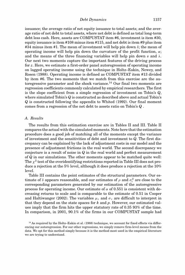
issuance; the average ratio of net equity issuance to total assets; and the aver-age ratio of net debt to total assets, where net debt is defined as total long-termdebt less cash. Here, assets are COMPUSTAT item #6, investment is item #30,equity issuance is item #108 minus item #115, and net debt is item #9 plus item#34 minus item #1. The mean of investment will help pin down δ; the mean ofoperating income will help pin down the curvature of the profit function, α;and the means of the three financing variables will help pin down s and λ.Our next two moments capture the important features of the driving processfor z. Here, we estimate a first-order panel autoregression of operating incomeon lagged operating income using the technique in Holtz–Eakin, Newey, andRosen (1988). Operating income is defined as COMPUSTAT item #13 dividedby item #6. The two moments that we match from this exercise are the au-toregressive parameter and the shock variance.14 Our final two moments areregression coefficients commonly calculated by empirical researchers. The firstis the slope coefficient from a simple regression of investment on Tobin’s Q,where simulated Tobin’s Q is constructed as described above and actual Tobin’sQ is constructed following the appendix to Whited (1992). Our final momentcomes from a regression of the net debt to assets ratio on Tobin’s Q .
A. Results
The results from this estimation exercise are in Tables II and III. Table IIcompares the actual with the simulated moments. Note here that the estimationprocedure does a good job of matching all of the moments except the varianceof investment and the sensitivities of debt and investment to Q. The first dis-crepancy can be explained by the lack of adjustment costs in our model and thepresence of adjustment frictions in the real world. The second discrepancy weconjecture is a result of noise in Q in the real world and perfect measurementof Q in our simulations. The other moments appear to be matched quite well:The χ2 test of the overidentifying restrictions reported in Table III does not pro-duce a rejection at the 5% level, although it does produce a rejection at the 10%level.
Table III contains the point estimates of the structural parameters. Our es-timate of δ appears reasonable, and our estimates of ρ and σ 2
ε are close to thecorresponding parameters generated by our estimation of the autoregressiveprocess for operating income. Our estimate of α of 0.551 is consistent with de-creasing returns to scale and is comparable to the estimate of 0.51 in Cooperand Haltiwanger (2002). The variables µτ and σ τ are difficult to interpret inthat they depend on the state spaces for k and p. However, our estimated val-ues imply that the firm hits the upper statutory rate of 0.35 93% of the time.In comparison, in 2001, 90.1% of the firms in our COMPUSTAT sample had
14 As required by the Holtz–Eakin et al. (1988) technique, we account for fixed effects via differ-encing our autoregression. For our other regressions, we simply remove firm-level means from thedata. We opt for this method simply because it is the method most used in the empirical literaturewe are trying to understand.
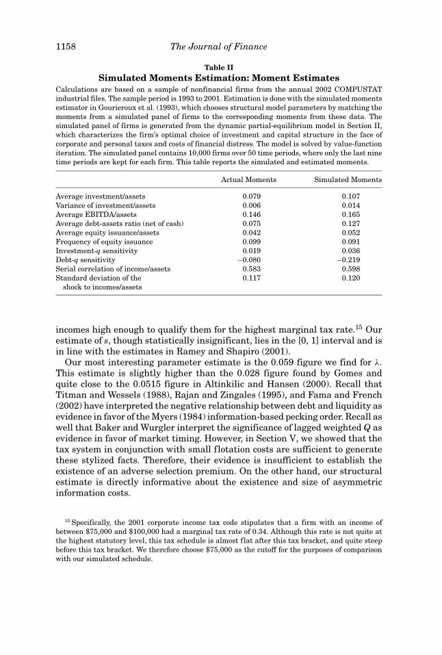
1158 The Journal of Finance
Table IISimulated Moments Estimation: Moment Estimates
Calculations are based on a sample of nonfinancial firms from the annual 2002 COMPUSTATindustrial files. The sample period is 1993 to 2001. Estimation is done with the simulated momentsestimator in Gourieroux et al. (1993), which chooses structural model parameters by matching themoments from a simulated panel of firms to the corresponding moments from these data. Thesimulated panel of firms is generated from the dynamic partial-equilibrium model in Section II,which characterizes the firm’s optimal choice of investment and capital structure in the face ofcorporate and personal taxes and costs of financial distress. The model is solved by value-functioniteration. The simulated panel contains 10,000 firms over 50 time periods, where only the last ninetime periods are kept for each firm. This table reports the simulated and estimated moments.
Actual Moments Simulated Moments
Average investment/assets 0.079 0.107Variance of investment/assets 0.006 0.014Average EBITDA/assets 0.146 0.165Average debt-assets ratio (net of cash) 0.075 0.127Average equity issuance/assets 0.042 0.052Frequency of equity issuance 0.099 0.091Investment-q sensitivity 0.019 0.036Debt-q sensitivity −0.080 −0.219Serial correlation of income/assets 0.583 0.598Standard deviation of the 0.117 0.120
shock to incomes/assets
incomes high enough to qualify them for the highest marginal tax rate.15 Ourestimate of s, though statistically insignificant, lies in the [0, 1] interval and isin line with the estimates in Ramey and Shapiro (2001).
Our most interesting parameter estimate is the 0.059 figure we find for λ.This estimate is slightly higher than the 0.028 figure found by Gomes andquite close to the 0.0515 figure in Altinkilic and Hansen (2000). Recall thatTitman and Wessels (1988), Rajan and Zingales (1995), and Fama and French(2002) have interpreted the negative relationship between debt and liquidity asevidence in favor of the Myers (1984) information-based pecking order. Recall aswell that Baker and Wurgler interpret the significance of lagged weighted Q asevidence in favor of market timing. However, in Section V, we showed that thetax system in conjunction with small flotation costs are sufficient to generatethese stylized facts. Therefore, their evidence is insufficient to establish theexistence of an adverse selection premium. On the other hand, our structuralestimate is directly informative about the existence and size of asymmetricinformation costs.
15 Specifically, the 2001 corporate income tax code stipulates that a firm with an income ofbetween $75,000 and $100,000 had a marginal tax rate of 0.34. Although this rate is not quite atthe highest statutory level, this tax schedule is almost flat after this tax bracket, and quite steepbefore this tax bracket. We therefore choose $75,000 as the cutoff for the purposes of comparisonwith our simulated schedule.
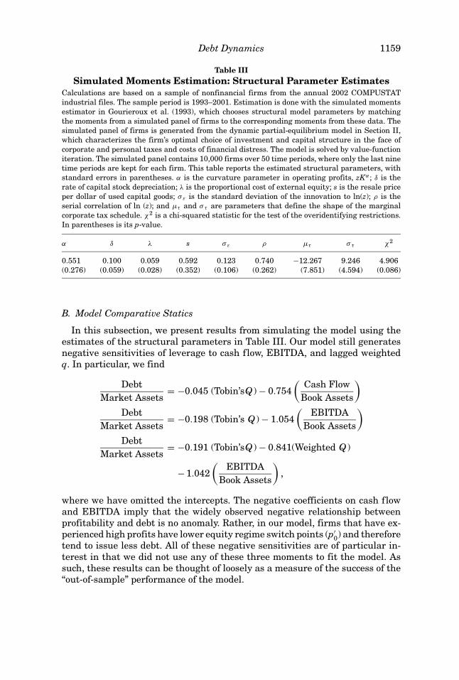
Debt Dynamics 1159
Table IIISimulated Moments Estimation: Structural Parameter Estimates
Calculations are based on a sample of nonfinancial firms from the annual 2002 COMPUSTATindustrial files. The sample period is 1993–2001. Estimation is done with the simulated momentsestimator in Gourieroux et al. (1993), which chooses structural model parameters by matchingthe moments from a simulated panel of firms to the corresponding moments from these data. Thesimulated panel of firms is generated from the dynamic partial-equilibrium model in Section II,which characterizes the firm’s optimal choice of investment and capital structure in the face ofcorporate and personal taxes and costs of financial distress. The model is solved by value-functioniteration. The simulated panel contains 10,000 firms over 50 time periods, where only the last ninetime periods are kept for each firm. This table reports the estimated structural parameters, withstandard errors in parentheses. α is the curvature parameter in operating profits, zKα ; δ is therate of capital stock depreciation; λ is the proportional cost of external equity; s is the resale priceper dollar of used capital goods; σε is the standard deviation of the innovation to ln(z); ρ is theserial correlation of ln (z); and µτ and σ τ are parameters that define the shape of the marginalcorporate tax schedule. χ2 is a chi-squared statistic for the test of the overidentifying restrictions.In parentheses is its p-value.
α δ λ s σε ρ µτ σ τ χ2
0.551 0.100 0.059 0.592 0.123 0.740 −12.267 9.246 4.906(0.276) (0.059) (0.028) (0.352) (0.106) (0.262) (7.851) (4.594) (0.086)
B. Model Comparative Statics
In this subsection, we present results from simulating the model using theestimates of the structural parameters in Table III. Our model still generatesnegative sensitivities of leverage to cash flow, EBITDA, and lagged weightedq. In particular, we find
DebtMarket Assets
= −0.045 (Tobin’sQ) − 0.754(
Cash FlowBook Assets
)Debt
Market Assets= −0.198 (Tobin’s Q) − 1.054
(EBITDA
Book Assets
)Debt
Market Assets= −0.191 (Tobin’sQ) − 0.841(Weighted Q)
− 1.042(
EBITDABook Assets
),
where we have omitted the intercepts. The negative coefficients on cash flowand EBITDA imply that the widely observed negative relationship betweenprofitability and debt is no anomaly. Rather, in our model, firms that have ex-perienced high profits have lower equity regime switch points (p′
0) and thereforetend to issue less debt. All of these negative sensitivities are of particular in-terest in that we did not use any of these three moments to fit the model. Assuch, these results can be thought of loosely as a measure of the success of the“out-of-sample” performance of the model.
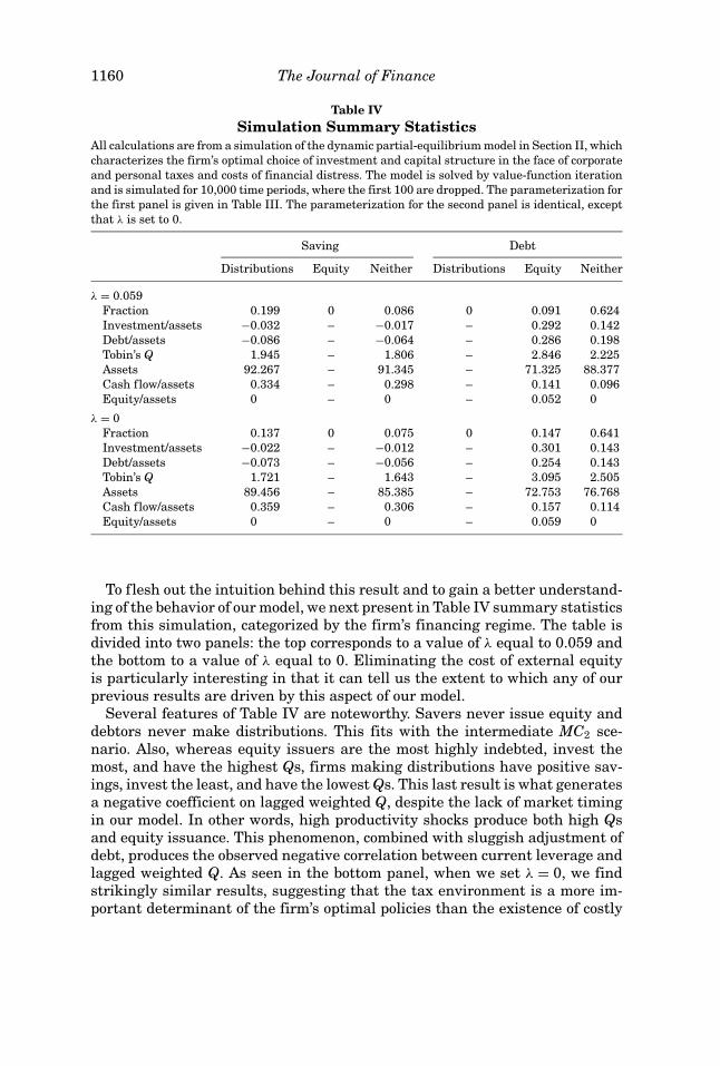
1160 The Journal of Finance
Table IVSimulation Summary Statistics
All calculations are from a simulation of the dynamic partial-equilibrium model in Section II, whichcharacterizes the firm’s optimal choice of investment and capital structure in the face of corporateand personal taxes and costs of financial distress. The model is solved by value-function iterationand is simulated for 10,000 time periods, where the first 100 are dropped. The parameterization forthe first panel is given in Table III. The parameterization for the second panel is identical, exceptthat λ is set to 0.
Saving Debt
Distributions Equity Neither Distributions Equity Neither
λ = 0.059Fraction 0.199 0 0.086 0 0.091 0.624Investment/assets −0.032 – −0.017 – 0.292 0.142Debt/assets −0.086 – −0.064 – 0.286 0.198Tobin’s Q 1.945 – 1.806 – 2.846 2.225Assets 92.267 – 91.345 – 71.325 88.377Cash flow/assets 0.334 – 0.298 – 0.141 0.096Equity/assets 0 – 0 – 0.052 0
λ = 0Fraction 0.137 0 0.075 0 0.147 0.641Investment/assets −0.022 – −0.012 – 0.301 0.143Debt/assets −0.073 – −0.056 – 0.254 0.143Tobin’s Q 1.721 – 1.643 – 3.095 2.505Assets 89.456 – 85.385 – 72.753 76.768Cash flow/assets 0.359 – 0.306 – 0.157 0.114Equity/assets 0 – 0 – 0.059 0
To flesh out the intuition behind this result and to gain a better understand-ing of the behavior of our model, we next present in Table IV summary statisticsfrom this simulation, categorized by the firm’s financing regime. The table isdivided into two panels: the top corresponds to a value of λ equal to 0.059 andthe bottom to a value of λ equal to 0. Eliminating the cost of external equityis particularly interesting in that it can tell us the extent to which any of ourprevious results are driven by this aspect of our model.
Several features of Table IV are noteworthy. Savers never issue equity anddebtors never make distributions. This fits with the intermediate MC2 sce-nario. Also, whereas equity issuers are the most highly indebted, invest themost, and have the highest Qs, firms making distributions have positive sav-ings, invest the least, and have the lowest Qs. This last result is what generatesa negative coefficient on lagged weighted Q, despite the lack of market timingin our model. In other words, high productivity shocks produce both high Qsand equity issuance. This phenomenon, combined with sluggish adjustment ofdebt, produces the observed negative correlation between current leverage andlagged weighted Q. As seen in the bottom panel, when we set λ = 0, we findstrikingly similar results, suggesting that the tax environment is a more im-portant determinant of the firm’s optimal policies than the existence of costly
Debt Dynamics 1161
external equity. The two major differences we do find occur in savings behaviorand equity issuance. As λ goes to zero, equity issuance naturally rises. Fur-ther, savings falls as the corporation’s precautionary motive diminishes. It doesnot disappear, however, because the firm still has a motive to save when τ c islow.
Note that under these parameters, the firm behaves in rough accordancewith the rules of thumb of the static pecking order theory. However, changesin the tax regime can lead to departures. We explore these possibilities via avariety of scenarios. First, we lower the maximal statutory corporate incometax rate until it is just above the tax rate on interest income. When we dothis, we find that the firm will finance solely with equity approximately 3%of the time. This violation of the static pecking order occurs for firms who arecurrent savers and who anticipate needing equity in the future. Second, whenwe lower the maximal corporate tax rate below the tax rate on interest income,we find, as predicted by the model in the high MC3 scenario, that the firmalways retains funds and only finances with equity. In other words, we find atax-based rationale for corporate liquidity holdings. This sort of phenomenoncan also occur in a firm that has, for example, high nondebt tax shields. Third,when we raise the maximal corporate income tax rate to 40%, the tax benefit ofdebt is sufficiently great that firms occasionally find it optimal to issue debt andmake distributions at the same time. This high corporate tax rate simulationalso generates some observations in which the firm has enough internal fundsto finance optimal investment, but nonetheless chooses to issue debt—a resultconsistent with the low MC1 scenario.
VII. Conclusion
In recent years, corporate finance economists have uncovered a variety of phe-nomena that appear anomalous in light of the traditional static trade-off theory.Our paper questions whether these phenomena are indeed anomalies. We do soby addressing the empirical observations from a more structural perspective.We begin by fully specifying a dynamic model of investment and finance. Weshow theoretically and via model simulations that there is no target leverageratio; firms can be savers or heavily levered; leverage is path dependent andexhibits hysteresis; leverage is decreasing in lagged cash flow and profitability;and leverage varies negatively with an external finance weighted average Q ra-tio. We also show that taxation does not have a “second order” effect on leveragedecisions. Indeed, even in the presence of a premium on external equity, we findthat variations in tax parameters have more power to explain anomalies thanthis premium. The key differences between our theory and its predecessorsare the simple ideas that firms make leverage decisions jointly with currentinvestment decisions and that this joint decision depends strongly on the cur-rent and anticipated financing margins. We also take the theory to the datawith a simulated moments estimator, finding that the cost of external equityfinance is a modest 5.9%, consistent with existing evidence on underwritingfees.
1162 The Journal of Finance
Overall, our theoretical and empirical results underline the importance ofunderstanding corporate financial decisions in dynamic settings, as well as theimportance of having a tight connection between theory and empirical work.Given the power of our theoretical and empirical framework to explain observedleverage phenomena, it appears likely that similar success is possible in otherareas of corporate finance.
Appendix
Proof of Proposition 1: The constraint correspondence for this problem isconstant-valued and, hence, continuous. The set K × P is nonempty and com-pact. Since e is a continuous function with compact domain, it is also bounded.Therefore, Assumptions 9.4–9.7 of Stokey and Lucas (SL) (1989) are satisfied.The result follows from SL Theorem 9.6. Q.E.D.
Proof of Proposition 2 and 3: To prove monotonicity, simply redefine theproblem by dropping the notation p and substituting the variable l ≡ −1 ∗ p.The equity value function in this case can be denoted v, and satisfies v(k, l, z) =V(k, p, z). The collateral constraint demands l ∈ L ≡ [−p(k), −p]. Since the con-straint set K × L is strictly increasing and the function e is strictly increasingin (k, l), SL Assumptions 9.4–9.9 are satisfied. SL Theorem 9.7 implies thatv(·, ·, z) is strictly increasing, from which it follows that V is strictly increasing(decreasing) in its first (second) argument.
The proof of concavity and uniqueness of the optimal policy follows SL The-orem 9.8. Assumptions 9.4–9.7 have been checked. Since K × P is convex, As-sumption 9.11 is also met. Thus, we need only check that Assumption 9.10,concavity of e(·, ·, ·, ·, z), is satisfied. To do so, we make use of the followingresult from Ziemba (1974) given as lemma A2 in his note.
LEMMA: Let y be a vector of m real variables and xi ≡ hi(y) for i = 1 , . . . , n bereal valued functions, with
f (y) ≡ u[h1(y), . . . , hn(y)].
If each hi is weakly concave; some hi, say hj, is strictly concave; u is weaklyconcave; u is nondecreasing; and u is strictly increasing in hj, then f (y) is strictlyconcave.
To use Ziemba’s lemma, note that we may write:
e(k, p, k′, p′, z) ≡ U [G1(k, p, z), G2(k, k′, p′)]
U (G1, G2) ≡ [1 + �iλ − �dτd ][G1 + G2]
G1(k, p, z) ≡ π (k, z) − g ( y(k, p, z)) − p�n + s�s
G2(k, k′, p′) ≡ k(1 − δ) − k′ + p′
1 + r.

Debt Dynamics 1163
We know that U is strictly increasing in both arguments; U is weakly concave;and G2 is weakly concave. Thus, to prove concavity of e, we must prove G1 isstrictly concave. To do so, note that we may write G1 as follows:
G1(k, p, z) ≡ u[ f (k, p, z)]
u( f ) ≡ f�n + s�s
f (k, p, z) ≡ π (k, z) − g ( y(k, p, z)) − p.
We know that u is strictly increasing in f and weakly concave. Thus, strictconcavity of f implies strict concavity of G1. The Hessian matrix for f (·, ·, z) isdenoted H:
H ≡[
fkk fkp
fkp fpp
].
The necessary conditions for strict concavity of f are satisfied with
|H1| = π11(1 − τc) − g ′′( y)(π1 − δ)2 < 0
|H2| = −(
r1 + r
)2
g ′′( y)π11(1 − τc) > 0.
With the signs of the determinants pinned down by π11 < 0 and g′′ > 0 fromAssumptions 1 and 6, respectively. Q.E.D.
Proof of Proposition 4: Follows from the Envelope Theorem of Benvenisteand Scheinkman (1979), applied as in the proof Theorem 9.10 in SL(1989). Q.E.D.
REFERENCESAlmeida, Heitor, Murillo Campello, and Michael S. Weisbach, 2004, The cash flow sensitivity of
cash, Journal of Finance 59, 1777–1804.Altinkilic, Oya, and Robert S. Hansen, 2000, Are there economies of scale in underwriting fees?
Evidence of rising external financing costs, Review of Financial Studies 13, 191–218.Asquith, Paul, Robert Gertner, and David Scharfstein, 1994, Anatomy of financial distress: An
examination of junk-bond issuers, Quarterly Journal of Economics 59, 625–658.Auerbach, Alan, 1979, Share valuation and corporate equity policy, Journal of Public Economics
11, 291–305.Auerbach, Alan, 2000, Taxation and corporate financial policy, in A. Auerbach and M. Feldstein,
eds.: Handbook of Public Economics (North Holland, Amsterdam).Baker, Malcolm, and Jeffrey Wurgler, 2002, Market timing and capital structure, Journal of
Finance 57, 1–32.Benveniste, Lawrence, and Jose Scheinkman, 1979, On the differentiability of the value function
in dynamic models of economics, Econometrica 47, 727–732.Bernanke, Ben, and Mark Gertler, 1989, Agency costs, net worth and business fluctuations, Amer-
ican Economic Review 79, 14–31.Bradford, David F., 1981, The incidence and allocation effects of a tax on corporate distributions,
Journal of Public Economics 15, 1–22.
1164 The Journal of Finance
Brennan, Michael J., and Eduardo S. Schwartz, 1984, Optimal financial policy and firm valuation,Journal of Finance 39, 593–607.
Clementi, Gian Luca, and Hugo A. Hopenhayn, 2002, A theory of financing constraints and firmdynamics, Working paper, Carnegie Mellon University.
Cooley, Thomas F., and Vincenzo Quadrini, 2001, Financial markets and firm dynamics, AmericanEconomic Review 91, 1286–1310.
Cooper, Russell, and Joao Ejarque, 2001, Exhuming Q: Market power vs. capital market imperfec-tions, Working Paper 8182, NBER.
Cooper, Russell, and John Haltiwanger, 2002, On the nature of capital adjustment costs, WorkingPaper 7925, NBER.
Duffie, Darrell, and Kenneth Singleton, 1999, Simulating correlated defaults, Working paper,Stanford University.
Erickson, Timothy, and Toni M. Whited, 2000, Measurement error and the relationship betweeninvestment and q, Journal of Political Economy 108, 1027–1057.
Fama, Eugene F., and Kenneth R. French, 2002, Testing trade-off and pecking order predictionsabout dividends and debt, Review of Financial Studies 15, 1–33.
Feldstein, Martin, and Lawrence Summers, 1979, Inflation and taxation of capital income in thecorporate sector, National Tax Journal 41, 219–233.
Fischer, Edwin O., Robert Heinkel, and Josef Zechner, 1989, Dynamic capital structure choice:Theory and tests, Journal of Finance 44, 19–40.
Goldstein, Robert, Nengjiu Ju, and Hayne Leland, 2001, An EBIT based model of dynamic capitalstructure, Journal of Business 74, 483–512.
Gomes, Joao F., 2001, Financing investment, American Economic Review 91, 1263–1285.Gourieroux, Christian, and Alain Monfort, 1996, Simulation Based Econometric Methods (Oxford
University Press, Oxford, U.K.).Gourieroux, Christian, Alain Monfort, and E. Renault, 1993, Indirect inference, Journal of Applied
Econometrics 8, S85–S118.Graham, John R., 1996a, Debt and the marginal tax rate, Journal of Financial Economics 41,
41–73.Graham, John R., 1996b, Proxies for the corporate marginal tax rate, Journal of Financial Eco-
nomics 42, 187–221.Graham, John R., 2000, How big are the tax benefits of debt? Journal of Finance 55, 1901–1941.Green, Richard, and Burton Hollifield, 2003, The personal tax advantages of equity, Journal of
Financial Economics, 67, 175–216.Holtz–Eakin, Douglas, Whitney K. Newey, and Harvey Rosen, 1988, Estimating vector autoregres-
sions with panel data, Econometrica 56, 1371–1395.Kim, Chang-Soo, David C. Mauer, and Ann E. Sherman, 1998, The determinants of corporate
liquidity: Theory and evidence, Journal of Financial and Quantitative Analysis 33, 335–359.
King, Mervin A., 1974, Taxation and the cost of capital, Review of Economic Studies 41, 21–35.Kiyotaki, Nobuhiro, and John Moore, 1997, Credit cycles, Journal of Political Economy 105, 211–
248.Leary, Mark, and Michael R. Roberts, 2004a, Do firms rebalance their capital structures? Working
paper, Duke University.Leary, Mark, and Michael R. Roberts, 2004b, Financial slack and tests of the pecking order theory
of capital structure, Working paper, Duke University.Leland, Hayne E., 1998, Agency costs, risk management, and capital structure, Journal of Finance
53, 1213–1243.Leland, Hayne E., and Klaus Bjerre Toft, 1996, Optimal capital structure, endogenous bankruptcy,
and the term structure of credit spreads, Journal of Finance 51, 987–1019.Lucas, Robert E., 1978, On the size distribution of business firms, Bell Journal of Economics 9,
508–523.MacKie-Mason, Jeffrey, 1990, Do taxes affect corporate financing decisions? Journal of Finance 45,
1471–1493.Miller, Merton, 1977, Debt and taxes, Journal of Finance 32, 261–275.
Debt Dynamics 1165
Michaelides, Alexander, and Serena Ng, 2000, Estimating the rational expectations model of spec-ulative storage: A Monte Carlo comparison of three simulation estimators, Journal of Econo-metrics 96, 231–266.
Mitchell, Mark, 2000, Debt policy at UST Inc., Harvard Business School Case 9-200-069.Modigliani, Franco, and Merton Miller, 1963, Corporate income taxes and the cost of capital: A
correction, American Economic Review 53, 433–443.Myers, Stewart C., 1984, The capital structure puzzle, Journal of Finance 39, 575–592.Myers, Stewart C., 1993, Still searching for optimal capital structure, Journal of Applied Corporate
Finance 6, 4–14.Pulvino, Todd, 1998, Do asset fire-sales exist? An empirical investigation of commercial aircraft
transactions, Journal of Finance 53, 939–978.Pulvino, Todd, 1999, Effects of bankruptcy court protection on asset sales, Journal of Financial
Economics 52, 151–186.Rajan, Raghuram G., and Luigi Zingales, 1995, What do we know about capital structure? Some
evidence from international data, Journal of Finance 50, 1421–1460.Ramey, Valerie A., and Matthew D. Shapiro, 2001, Displaced capital: A study of aerospace plant
closings, Journal of Political Economy 109, 958–992.Schurhoff, Norman, 2004, Capital gains taxes, irreversible investment, and capital structure, Work-
ing paper, Carnegie Mellon University.Shyam-Sunder, Lakshmi, and Stewart C. Myers, 1999, Testing static trade-off against pecking
order models of capital structure, Journal of Financial Economics 51, 219–244.Sinn, Hans Werner, 1991, The vanishing harberger triangle, Journal of Public Economics 45, 271–
300.Smith, Clifford W. Jr., 1977, Alternative methods for raising capital: Rights versus underwritten
offerings, Journal of Financial Economics 5, 273–307.Stiglitz, Joseph E., 1973, Taxation, corporate financial policy, and the cost of capital, Journal of
Public Economics 5, 303–311.Stiglitz, Joseph E., and Andrew Weiss, 1981, Credit rationing in markets with imperfect informa-
tion, American Economic Review, 393–410.Stokey, Nancy L., and Robert E. Lucas, 1989, Recursive Methods in Economic Dynamics (Harvard
University Press, Cambridge, MA).Strebulaev, Ilya, 2004, Do tests of capital structure theory mean what they say? Working paper,
London Business School.Tauchen, George, 1986, Finite state Markov-chain approximations to univariate and vector autore-
gressions, Economics Letters 20, 177–181.Titman, Sheridan, and Sergey Tsyplakov, 2003, A dynamic model of optimal capital structure,
Working paper, University of Texas at Austin.Titman, Sheridan, and Roberto Wessels, 1988, The determinants of capital structure choice, Jour-
nal of Finance 43, 1–21.Whited, Toni M., 1992, Debt, liquidity constraints, and corporate investment: Evidence from panel
data, Journal of Finance 47, 1425–1460.Ziemba, William T., 1974, The behavior of a firm subject to stochastic regulatory review: Comment,
Bell Journal of Economics and Management Science 5, 710–712.
Related Documents