University of Central Florida University of Central Florida STARS STARS Electronic Theses and Dissertations, 2004-2019 2006 Debris Characterization And Mitigation Of Droplet Laser Plasma Debris Characterization And Mitigation Of Droplet Laser Plasma Sources For Euv Lithography Sources For Euv Lithography Kazutoshi Takenoshita University of Central Florida Part of the Electrical and Electronics Commons Find similar works at: https://stars.library.ucf.edu/etd University of Central Florida Libraries http://library.ucf.edu This Doctoral Dissertation (Open Access) is brought to you for free and open access by STARS. It has been accepted for inclusion in Electronic Theses and Dissertations, 2004-2019 by an authorized administrator of STARS. For more information, please contact [email protected]. STARS Citation STARS Citation Takenoshita, Kazutoshi, "Debris Characterization And Mitigation Of Droplet Laser Plasma Sources For Euv Lithography" (2006). Electronic Theses and Dissertations, 2004-2019. 917. https://stars.library.ucf.edu/etd/917

Welcome message from author
This document is posted to help you gain knowledge. Please leave a comment to let me know what you think about it! Share it to your friends and learn new things together.
Transcript

University of Central Florida University of Central Florida
STARS STARS
Electronic Theses and Dissertations, 2004-2019
2006
Debris Characterization And Mitigation Of Droplet Laser Plasma Debris Characterization And Mitigation Of Droplet Laser Plasma
Sources For Euv Lithography Sources For Euv Lithography
Kazutoshi Takenoshita University of Central Florida
Part of the Electrical and Electronics Commons
Find similar works at: https://stars.library.ucf.edu/etd
University of Central Florida Libraries http://library.ucf.edu
This Doctoral Dissertation (Open Access) is brought to you for free and open access by STARS. It has been accepted
for inclusion in Electronic Theses and Dissertations, 2004-2019 by an authorized administrator of STARS. For more
information, please contact [email protected].
STARS Citation STARS Citation Takenoshita, Kazutoshi, "Debris Characterization And Mitigation Of Droplet Laser Plasma Sources For Euv Lithography" (2006). Electronic Theses and Dissertations, 2004-2019. 917. https://stars.library.ucf.edu/etd/917
DEBRIS CHARACTERIZATION AND MITIGATION OFDROPLET LASER PLASMA SOURCES FOR EUV LITHOGRAPHY
by
KAZUTOSHI TAKENOSHITABachelors degree in Electric and Electronic Engineering
Niigata University, Niigata, Japan, 1994Masters degree in Electric and Electronic Engineering
Niigata University, Niigata, Japan, 1996
A dissertation submitted in partial fulfillment of the requirementsfor the degree of Doctor of Philosophy
in the Department of Electrical Engineeringin the School of Electrical Engineering and Computer Science
at the University of Central FloridaOrlando, Florida
Summer Term2006
Major Professor: Martin C Richardson

c© 2006 Kazutoshi Takenoshita
ii

ABSTRACT
Extreme ultraviolet lithography (EUVL) is a next generation lithographic techniques
under development for fabricating semiconductor devices with feature sizes smaller than 32
nm. The optics to be used in the EUVL steppers is reflective optics with multilayer mirror
coatings on each surface. The wavelength of choice is 13.5 nm determined by the optimum
reflectivity of the mirror coatings. The light source required for this wavelength is derived
from a hot-dense plasma produced by either a gas discharge or a laser. This study concentrate
only on the laser produced plasma source because of its advantages of scalability to higher
repetition rates.
The design of a the laser plasma EUVL light source consists of a plasma produced
from a high-intensity focused laser beam from a solid/liquid target, from which radiation
is generated and collected by a large solid angle mirror or array of mirrors. The collector
mirrors have the same reflectivity characteristics as the stepper mirrors. The EUVL light
source is considered as the combination of both the hot-dense plasma and the collector
mirrors.
The EUVL light sources required by the stepper manufacturers must have sufficient
EUV output power and long operational lifetimes to meet market-determined chip produc-
tion rates. The most influential factor in achieving the required EUV output power is the
conversion efficiency (CE) of laser input energy relative to the EUV radiation collected. A
high CE is demonstrated in a separate research program by colleagues in the Laser Plasma
laboratory at CREOL. Another important factor for the light source is the reflectivity life-
time of the collection optics as mirror reflectivity can be degraded by deposition and ablation
from the plasma debris. Realization of a high CE but low debris plasma source is possible by
iii

reducing the mass of the target, which is accomplished by using tin-doped droplet targets.
These have sufficient numbers of tin atoms for high CE, but the debris generation is minimal.
The first part of this study investigates debris emissions from tin-doped droplet tar-
gets, in terms of aerosols and ions. Numerous tin aerosols can be created during a single
laser-target interaction. The effects these interactions are observed and the depositions are
investigated using SEM, AFM, AES, XPS, and RBS techniques. The generation of aerosols
is found to be the result of incomplete ionization of the target material, corresponding to
non-optimal laser coupling to the target for maximum CE. In order to determine the threats
of the ion emission to the collector mirror coatings from an optimal, fully ionized target, the
ion flux is measured at the mirror distance using various techniques. The ion kinetic energy
distributions obtained for individual ion species are quantitatively analyzed. Incorporating
these distributions with Monte-Carlo simulations provide lifetime estimation of the collec-
tor mirror under the effect of ion sputtering. The current estimated lifetime the tin-doped
droplet plasma source is only a factor of 500 less than the stepper manufacturer require-
ments, without the use of any mitigation schemes to stop these ions interacting with the
mirror.
The second part of this investigation explores debris mitigation schemes. Two miti-
gation schemes are applied to tin-doped droplet laser plasmas; electrostatic field mitigation,
and a combination of a foil trap with a magnetic field. Both mitigation schemes demonstrate
their effectiveness in suppressing aerosols and ion flux. A very small number of high-energy
ions still pass through the combination of the two mitigation schemes but the sputtering
caused by these ions is too small to offer a threat to mirror lifetime. It is estimated that
the lifetime of the collector mirror, and hence the source lifetime, will be sufficient when
tin-doped targets are used in combination with these mitigation schemes.
iv
ACKNOWLEDGMENTS
I would like to take a moment to express great appreciations to those who have
supported this study. Without them, this study would have never been completed as it is
now. I would like to thank first, Dr. Martin Richardson for providing this opportunity,
advising this study, and stimulating my scientific and engineering curiosity. I would also like
to thank all the committee members for valuable contributions, Dr. Kalpathy Sundaram,
Dr. Aravinda Kar, Dr. Donald Malocha for discussing the possibilities of SAW detectors,
and Dr. William Silfvast for discussing on the fundamentals of laser plasmas. In addition, I
would also like to thank Dr. David Attwood for encouraging me in the EUV research and
contributing this thesis.
I am very fortunate to join the Laser Plasma Laboratory where I meet fine scientists
and students from all different countries. For the droplet laser plasma generation, Dr. Chris-
tian Keyser, and Dr. Chiew-Seng Koay, because of their previous work, this study has its own
meaning. I have gained precious help from, as well as a lot of knowledge through discussions
with, Ms. Simi George, Mr. Tobias Schmid, Mr. Teddy Peponnet, Mr. Robert Bernath,
Mr. Joshua Duncan, Mr. Somsak Teerawattanasook, Mr. Jose Cunado, Ms. Ji-Yeon Choi,
and all the colleagues.
I like to thank the people in CREOL who discussed with me in the research, laser
plasmas, lasers and optics, especially Dr. Grag Shimkaveg, Dr. Etsuo Fujiwara, Dr. Nikolai
Vorobiev, Mr. Isao Matsubara, Dr. Sebastian Gauza, Dr. Fumiyo Yoshino, Dr. Yung-
Hsun Wu, and Dr. Yi-Hsin Lin. In addition, there are many scientist outside school gave me
valuable inputs in different universities, organizations, and companies, especially Mr Yasuaki
Fukuda and Dr.Kazuaki Hotta for explaining the whole picture of the lithography industry.
v

I have kept a strong desire in my mind towards the application of the droplet gener-
ations. It is my turn to contribute to those who worked together in Silver Seiko Ltd. and
Siemens-Elema AB. where I have gained all varieties of knowledge and techniques that I
can apply throughout the study. I like especially to express my appreciation to Dr. Milan
Pokorny for all the initiations and his friendship, Mr. Ulf Fahlstrom for supporting and his
friendship, Dr. Masayuki Muto, Mr. Shizuo Terashima, Mr. Takeshi Fujiwara, Mr. Kunio
Takahashi, for giving me the opportunities for the SRjet printing head development.
This study is also a result of all the support I have had from friends and family. Dr.
Takeo Maruyama and Mrs. Makiko Maruyama, Mr. Masaki Uesugi, and all the friends in
Niigata city and Kashiwazaki city have been supporting and encouraging me and my wife,
Miyuki. Dr. Calvin Hayes and Mrs. Barbara Hayes have been encouraging me and believed
in me for pursuing this study. My parents and parents-in-low have been very supportive and
waiting for me to complete the study. Lastly I thank my wife, Miyuki, for supporting me in
here in the states. She should receive my most appreciation.
vi

TABLE OF CONTENTS
LIST OF FIGURES . . . . . . . . . . . . . . . . . . . . . . . . . . . . . . . . . xvii
LIST OF TABLES . . . . . . . . . . . . . . . . . . . . . . . . . . . . . . . . . .xviii
LIST OF ACRONYMS/ABBREVIATIONS . . . . . . . . . . . . . . . . . . xix
CHAPTER 1 INTRODUCTION . . . . . . . . . . . . . . . . . . . . . . . . 1
1.1 EUV Lithography . . . . . . . . . . . . . . . . . . . . . . . . . . . . . . . . . 1
1.1.1 Overview of EUVL . . . . . . . . . . . . . . . . . . . . . . . . . . . . 3
1.1.2 EUVL source requirement . . . . . . . . . . . . . . . . . . . . . . . . 4
1.1.3 Conversion efficiency . . . . . . . . . . . . . . . . . . . . . . . . . . . 5
1.1.4 Source lifetime . . . . . . . . . . . . . . . . . . . . . . . . . . . . . . 6
1.2 EUV - Soft X-ray sources . . . . . . . . . . . . . . . . . . . . . . . . . . . . 7
1.2.1 Synchrotron radiation . . . . . . . . . . . . . . . . . . . . . . . . . . 8
1.2.2 Gas discharge dense plasmas . . . . . . . . . . . . . . . . . . . . . . . 9
1.2.3 Laser plasmas . . . . . . . . . . . . . . . . . . . . . . . . . . . . . . . 10
1.3 Multilayer mirror coating and reflectivity . . . . . . . . . . . . . . . . . . . . 12
1.3.1 Absorption of soft X-ray in materials . . . . . . . . . . . . . . . . . . 12
1.3.2 Reflectivity of multi-layer mirror . . . . . . . . . . . . . . . . . . . . 13
1.4 Summary of background and motivation . . . . . . . . . . . . . . . . . . . . 15
CHAPTER 2 LASER PLASMAS AND DEBRIS . . . . . . . . . . . . . . . 17
2.1 Introduction . . . . . . . . . . . . . . . . . . . . . . . . . . . . . . . . . . . . 17
vii

2.1.1 Laser Plasma generation . . . . . . . . . . . . . . . . . . . . . . . . . 18
2.1.2 Absorption of laser energy in fully ionized plasmas . . . . . . . . . . . 18
2.1.3 Ionization stages . . . . . . . . . . . . . . . . . . . . . . . . . . . . . 20
2.1.4 Fluid descriptions of laser plasmas . . . . . . . . . . . . . . . . . . . 23
2.1.5 Plasma expansion . . . . . . . . . . . . . . . . . . . . . . . . . . . . . 25
2.1.6 Recombination . . . . . . . . . . . . . . . . . . . . . . . . . . . . . . 26
2.2 Debris generation . . . . . . . . . . . . . . . . . . . . . . . . . . . . . . . . . 26
2.2.1 Solid target and debris . . . . . . . . . . . . . . . . . . . . . . . . . . 27
2.2.2 Hot rocks and aerosols . . . . . . . . . . . . . . . . . . . . . . . . . . 28
2.2.3 Ions, electrons, and neutral atoms . . . . . . . . . . . . . . . . . . . . 29
2.3 Mass-limited target . . . . . . . . . . . . . . . . . . . . . . . . . . . . . . . . 30
2.3.1 Different target configurations . . . . . . . . . . . . . . . . . . . . . . 30
2.3.2 Number of atoms in a target . . . . . . . . . . . . . . . . . . . . . . . 32
2.4 Summary of laser plasmas and debris generation . . . . . . . . . . . . . . . . 34
CHAPTER 3 MULTILAYER MIRROR REFLECTIVITY DEGRADATION 35
3.1 Introduction . . . . . . . . . . . . . . . . . . . . . . . . . . . . . . . . . . . . 35
3.2 Deposition . . . . . . . . . . . . . . . . . . . . . . . . . . . . . . . . . . . . . 35
3.2.1 EUV absorption of target materials . . . . . . . . . . . . . . . . . . . 36
3.2.2 Absorption estimates of thin film . . . . . . . . . . . . . . . . . . . . 37
3.2.3 Oxidation of multi-layer mirror surfaces . . . . . . . . . . . . . . . . . 39
3.2.4 Absorption of an oxide layers . . . . . . . . . . . . . . . . . . . . . . 39
3.2.5 Photon induced oxidation processes . . . . . . . . . . . . . . . . . . . 40
3.2.6 Impact on oxidation on collector mirror surfaces . . . . . . . . . . . . 41
3.3 Erosion on multi-layer surfaces . . . . . . . . . . . . . . . . . . . . . . . . . . 43
viii

3.3.1 Surface sputtering process . . . . . . . . . . . . . . . . . . . . . . . . 44
3.3.2 A Monte Carlo Simulation - SRIM . . . . . . . . . . . . . . . . . . . 45
3.3.3 Multilayer mirror reflectivity characteristics . . . . . . . . . . . . . . 45
3.4 Summary of multilayer mirror reflectivity degradation . . . . . . . . . . . . . 46
CHAPTER 4 EXPERIMENTAL FACILITIES . . . . . . . . . . . . . . . . 48
4.1 Introduction . . . . . . . . . . . . . . . . . . . . . . . . . . . . . . . . . . . . 48
4.2 Experimental facility . . . . . . . . . . . . . . . . . . . . . . . . . . . . . . . 48
4.2.1 High repetition rate (100Hz) Nd:YAG laser sytem . . . . . . . . . . . 48
4.2.2 The target chamber . . . . . . . . . . . . . . . . . . . . . . . . . . . . 49
4.2.3 Target delivery . . . . . . . . . . . . . . . . . . . . . . . . . . . . . . 51
4.2.4 Target laser synchronization . . . . . . . . . . . . . . . . . . . . . . . 52
4.3 Debris diagnostics . . . . . . . . . . . . . . . . . . . . . . . . . . . . . . . . . 54
4.3.1 Witness plate capture and post shot analysis . . . . . . . . . . . . . . 55
4.3.2 Deposition monitor . . . . . . . . . . . . . . . . . . . . . . . . . . . . 57
4.3.3 Faraday cup ion probes . . . . . . . . . . . . . . . . . . . . . . . . . . 57
4.3.4 Ion spectrometer with electrostatic ion energy analyzer . . . . . . . . 58
4.3.5 Thomson parabola spectrometer . . . . . . . . . . . . . . . . . . . . . 60
4.3.6 Amplified ion probe . . . . . . . . . . . . . . . . . . . . . . . . . . . . 61
4.4 Mitigation schemes . . . . . . . . . . . . . . . . . . . . . . . . . . . . . . . . 62
4.4.1 Electrostatic field mitigation . . . . . . . . . . . . . . . . . . . . . . . 63
4.4.2 Magnetic foil trap mitigation . . . . . . . . . . . . . . . . . . . . . . 64
4.5 Summary of experimental facilities . . . . . . . . . . . . . . . . . . . . . . . 67
CHAPTER 5 PARTICULATE DEBRIS - AEROSOLS . . . . . . . . . . . 68
ix

5.1 Introduction . . . . . . . . . . . . . . . . . . . . . . . . . . . . . . . . . . . . 68
5.2 Aerosol deposition on witness plates . . . . . . . . . . . . . . . . . . . . . . . 68
5.2.1 Identification of the deposits . . . . . . . . . . . . . . . . . . . . . . . 69
5.2.2 Profile measurement of the deposits . . . . . . . . . . . . . . . . . . . 71
5.2.3 Aerosol flux calculation . . . . . . . . . . . . . . . . . . . . . . . . . . 72
5.3 Aerosol generation processes . . . . . . . . . . . . . . . . . . . . . . . . . . . 74
5.3.1 Aerosol generation in low intensity laser irradiation . . . . . . . . . . 74
5.3.2 Origin of aerosol generation . . . . . . . . . . . . . . . . . . . . . . . 75
5.3.3 Laser energy, intensity, focus diameter . . . . . . . . . . . . . . . . . 77
5.3.4 Total tin atom emission . . . . . . . . . . . . . . . . . . . . . . . . . 78
5.4 Summary of particulate debris . . . . . . . . . . . . . . . . . . . . . . . . . . 79
CHAPTER 6 ION EMISSION . . . . . . . . . . . . . . . . . . . . . . . . . . 80
6.1 Introduction . . . . . . . . . . . . . . . . . . . . . . . . . . . . . . . . . . . . 80
6.2 Ion emission characteristics . . . . . . . . . . . . . . . . . . . . . . . . . . . . 80
6.2.1 Ion flux measurement . . . . . . . . . . . . . . . . . . . . . . . . . . . 81
6.2.2 Mass spectrometer . . . . . . . . . . . . . . . . . . . . . . . . . . . . 82
6.2.3 Quantitative ion spectrometer analysis . . . . . . . . . . . . . . . . . 84
6.2.4 Emission dependency on the laser intensities . . . . . . . . . . . . . . 91
6.3 Erosion study . . . . . . . . . . . . . . . . . . . . . . . . . . . . . . . . . . . 95
6.3.1 Limitation of laser repetition rate . . . . . . . . . . . . . . . . . . . . 95
6.3.2 Lifetime estimation of mirror reflectivity degradation . . . . . . . . . 96
6.4 Plasma expansion simulation . . . . . . . . . . . . . . . . . . . . . . . . . . . 98
6.4.1 Simplified model of fluid simulations . . . . . . . . . . . . . . . . . . 99
6.4.2 MEDUSA plasma expansion simulations . . . . . . . . . . . . . . . . 101
x

6.4.3 Comparison between simulations and ion measurements . . . . . . . . 106
6.5 Summary of ion emission characteristics . . . . . . . . . . . . . . . . . . . . 111
CHAPTER 7 MITIGATION . . . . . . . . . . . . . . . . . . . . . . . . . . . 112
7.1 Introduction . . . . . . . . . . . . . . . . . . . . . . . . . . . . . . . . . . . . 112
7.1.1 Types of mitigation schemes . . . . . . . . . . . . . . . . . . . . . . . 112
7.2 Repeller field mitigation . . . . . . . . . . . . . . . . . . . . . . . . . . . . . 113
7.2.1 Effectiveness of repeller field on ion flux . . . . . . . . . . . . . . . . 114
7.2.2 Effectiveness of repeller field on aerosols . . . . . . . . . . . . . . . . 118
7.3 Magnetic foil trap mitigation . . . . . . . . . . . . . . . . . . . . . . . . . . . 120
7.3.1 Particle motion in the magnetic field and foil structures . . . . . . . . 121
7.3.2 Particle motion in non-uniform magnetic field . . . . . . . . . . . . . 126
7.3.3 Effectiveness of foil trap mitigation . . . . . . . . . . . . . . . . . . . 127
7.4 Combination of two mitigation schemes . . . . . . . . . . . . . . . . . . . . . 129
7.4.1 Detection limit of ion flux . . . . . . . . . . . . . . . . . . . . . . . . 130
7.4.2 Demonstration of sufficient ion flux reduction . . . . . . . . . . . . . 133
7.4.3 Neutral atom mitigation . . . . . . . . . . . . . . . . . . . . . . . . . 134
7.5 Summary of mitigation . . . . . . . . . . . . . . . . . . . . . . . . . . . . . . 134
CHAPTER 8 CONCLUSION AND FUTURE WORK . . . . . . . . . . . 136
8.1 Conclusion . . . . . . . . . . . . . . . . . . . . . . . . . . . . . . . . . . . . . 136
8.2 Future work . . . . . . . . . . . . . . . . . . . . . . . . . . . . . . . . . . . . 137
8.2.1 High repetition rate laser plasmas . . . . . . . . . . . . . . . . . . . . 137
8.2.2 Target stabilization systems . . . . . . . . . . . . . . . . . . . . . . . 138
8.2.3 Radiation study under magnetic field existence . . . . . . . . . . . . . 138
xi

8.2.4 Temporary and spatially resolved spectroscopy . . . . . . . . . . . . . 139
8.2.5 Pre-pulse and post pulse heating . . . . . . . . . . . . . . . . . . . . 139
APPENDIX A ION KINETIC ENERGY DISTRIBUTIONS . . . . . . . . 141
APPENDIX B SIMPLIFIED FLUID DESCRIPTION OF PLASMA SIMU-
LATION . . . . . . . . . . . . . . . . . . . . . . . . . . . . . . . . . . . . . . 146
B.1 Class declaration . . . . . . . . . . . . . . . . . . . . . . . . . . . . . . . . . . 147
B.2 1D Process routine (method) . . . . . . . . . . . . . . . . . . . . . . . . . . . 149
REFERENCES . . . . . . . . . . . . . . . . . . . . . . . . . . . . . . . . . . . . 152
xii

LIST OF FIGURES
1.1 A general schematic of optical component layout of EUVL stepper machines
[9]. . . . . . . . . . . . . . . . . . . . . . . . . . . . . . . . . . . . . . . . . . 4
1.2 Schematic of synchrotron radiation [16]. . . . . . . . . . . . . . . . . . . . . 9
1.3 Schematic of gas discharge plasma source configuration [21]. . . . . . . . . . 10
1.4 An example of laser plasma EUV source, mirror, and IF configuration [22]. . 11
1.5 TEM cross section image of Mo/Si multilayer mirror surface [24]. . . . . . . 14
1.6 Reflectivity characteristics of Si/Mo multilayer coatings [25]. . . . . . . . . . 15
2.1 Ionization rate calculation at different electron densities. . . . . . . . . . . . 22
2.2 Population of tin ion species as function of electron temperature. . . . . . . . 23
2.3 Comparison of multilayer mirror surfaces exposed by Li and Sn plasmas [47]. 29
3.1 Absorption coefficient of Li, Sn, and Xe. . . . . . . . . . . . . . . . . . . . . 37
3.2 Transmission of thin film 10 nm of Si, Nb, Ru, Li, and Sn [25]. . . . . . . . . 38
3.3 Transmission of oxide layers [25]. . . . . . . . . . . . . . . . . . . . . . . . . 40
3.4 Mirror reflectivity degradation characteristics measured [66]. . . . . . . . . . 42
3.5 SEM image of a multilayer mirror surface showing the evidence of the erosion
caused by high energy oxygen ions [76]. . . . . . . . . . . . . . . . . . . . . . 44
3.6 Si/Mo multilayer mirror reflectivity characteristics of different number of bi-
layers [25]. . . . . . . . . . . . . . . . . . . . . . . . . . . . . . . . . . . . . . 46
4.1 Photo of the laser system . . . . . . . . . . . . . . . . . . . . . . . . . . . . . 49
4.2 Photo of target chamber . . . . . . . . . . . . . . . . . . . . . . . . . . . . . 50
xiii

4.3 Schematic of optical setting on the target chamber . . . . . . . . . . . . . . . 51
4.4 Orientations of target delivery, cold trap, heating laser pulse, imaging system,
and a visible image of the plasma observed by the imaging system. . . . . . . 53
4.5 Timing diagram of droplet and laser synchronization . . . . . . . . . . . . . 54
4.6 Experimental setup for (top) witness plate and (bottom) sample holder . . . 56
4.7 Schematic of Faraday cup ion probe . . . . . . . . . . . . . . . . . . . . . . . 58
4.8 Schematic of (ESIEA) ion spectrometer . . . . . . . . . . . . . . . . . . . . . 59
4.9 (a) Schematic of TPS, (b) Ion signals measured by TPS . . . . . . . . . . . . 61
4.10 Schematic of amplified ion probe . . . . . . . . . . . . . . . . . . . . . . . . 62
4.11 Concept of repeller field mitigation . . . . . . . . . . . . . . . . . . . . . . . 63
4.12 IP, ESIEA measurements with the repeller field, and witness plate measure-
ment with the repeller field. . . . . . . . . . . . . . . . . . . . . . . . . . . . 64
4.13 Schematic of magnetic foil trap single channel experiment . . . . . . . . . . . 66
4.14 Photos of magnetic foil trap single channel experiment setup (left) the mag-
netic core, (right) single channel foil. . . . . . . . . . . . . . . . . . . . . . . 66
5.1 (a) Auger electron spectrum taken from the witness plate and (b) X-ray pho-
toelectron spectrum taken from the same plate sample. . . . . . . . . . . . . 70
5.2 AES Sn signal comparison on the deposited aerosol. . . . . . . . . . . . . . . 71
5.3 AFM image of tin deposition on a multilayer mirror. . . . . . . . . . . . . . 72
5.4 Deposit volume dependency of the diameters. . . . . . . . . . . . . . . . . . 73
5.5 (a) AES image 140µm X 140µm, (b) Back-scattered image (Same area). . . . 74
5.6 (a) distances of target, mask, and witness plate, (b) dark field image of the
witness plate surface. . . . . . . . . . . . . . . . . . . . . . . . . . . . . . . . 76
xiv

5.7 (a) SEM image of witness plate surface exposed by plasma created by 30 mJ
laser pulse, (b) by 120 mJ pulse. . . . . . . . . . . . . . . . . . . . . . . . . . 77
6.1 Ion probe signals measured at 150mm from the plasma. . . . . . . . . . . . . 81
6.2 Ion probe signal from solid tin planer target. . . . . . . . . . . . . . . . . . . 82
6.3 (a) Ion spectrum and ion probe signal from water droplet target, (b) Ion
spectrum and ion probe signal from Tin 30% doped droplet target. . . . . . 83
6.4 (a) Typical ESIEA signal, (b) converted M/Z signal. . . . . . . . . . . . . . 86
6.5 (a) Collected M/Z signals, (b) interpolated M/Z spectral map. . . . . . . . . 87
6.6 Detailed schematics of ESIEA for quantitative analysis. . . . . . . . . . . . . 88
6.7 Tin ions energy distributions at intensity of 9.7 x 10¹⁰ W/cm2. . . . . . . . . 90
6.8 Ion probe signals at different laser intensities at 125 mm distance from the
plasma. . . . . . . . . . . . . . . . . . . . . . . . . . . . . . . . . . . . . . . 91
6.9 Ion kinetic energy distributions of (a) O+, (b) O2+, (c), and O5+. . . . . . . 93
6.10 Ion kinetic energy distributions of (a) Sn+, (b) Sn2+, (c), and Sn5+. . . . . . 94
6.11 The incident ion energy dependencies of the sputtering yields for Si, Mo sur-
faces. (SRIM calculations) . . . . . . . . . . . . . . . . . . . . . . . . . . . . 97
6.12 Concept of cells and properties of the simplified fluid model. . . . . . . . . . 100
6.13 Electron density and temperature profiles calculated by the simplified fluid
model at 2 ns of 10 ns, 100 mJ Gaussian laser pulse. . . . . . . . . . . . . . . 101
6.14 Medusa calculations of electron density and temperature transient at laser
intensity of 1.0 x 10¹¹ W/cm2. . . . . . . . . . . . . . . . . . . . . . . . . . . 103
6.15 Medusa calculations of electron density and temperature transient at laser
intensity of 2.0 x 10¹¹ W/cm2. . . . . . . . . . . . . . . . . . . . . . . . . . . 104
xv
6.16 Medusa calculations of electron density and temperature transient at laser
intensity of 3.0 x 10¹¹ W/cm2. . . . . . . . . . . . . . . . . . . . . . . . . . . 105
6.17 Comparisons of ion probe signal and electron density transient at (a) intensity
of 2.0 x 10¹¹ W/cm2, (b) 3.0 x 10¹¹W/cm2. . . . . . . . . . . . . . . . . . . . 107
6.18 Reconstructed ion signals of total signals and individual elements at laser
intensities of (a) 1.9 x 10¹¹, (b) 2.8 x 10¹¹ W/cm2. . . . . . . . . . . . . . . . 109
6.19 Reconstructed ion signals at laser intensities of 2.8 x 10¹¹ W/cm2. (a) Oxygen
ions, and (b) tin ions . . . . . . . . . . . . . . . . . . . . . . . . . . . . . . . 110
7.1 Comparison of IP signals with repeller field and without the field. . . . . . . 115
7.2 Ion M/Z spectral analysis on the repeller field effectiveness. . . . . . . . . . . 117
7.3 (a) Secondary electron image of 50µm x 50µm of surface exposed without
the repeller field, (b) Secondary electron image of 50µm x 50µm of surface
exposed with the repeller field, (c) Auger electron tin elemental mapping of
the same area as (a), (d) Tin elemental mapping of the same area as (b). . . 119
7.4 An example of the magnetic foil trap configuration. . . . . . . . . . . . . . . 120
7.5 Relationships between Φ and R under a uniform magnetic field. . . . . . . . 124
7.6 The illustration of the critical ion trajectory and foils. . . . . . . . . . . . . . 124
7.7 Ion deflection rates of (a) tin ion species under uniform magnetic field of 0.1 T
(b) different ion species under uniform magnetic field of 0.1 T (c) Sn+ under
different magnetic field. . . . . . . . . . . . . . . . . . . . . . . . . . . . . . . 125
7.8 Measured magnetic field profile on foil channel plane. . . . . . . . . . . . . . 127
7.9 IP measurement with magnetic foil trap for (a) water droplet target case, (b)
tin-doped droplet target case. . . . . . . . . . . . . . . . . . . . . . . . . . . 128
7.10 Photo and schematic of modified encapsulated repeller field mitigation. . . . 130
xvi
7.11 IP signal comparison between different field potentials of the modified Repeller
Field. . . . . . . . . . . . . . . . . . . . . . . . . . . . . . . . . . . . . . . . . 132
7.12 IP signals on the modified Magnetic Foil Trap. . . . . . . . . . . . . . . . . . 132
7.13 Amplified ion probe signals with two mitigation schemes installed. . . . . . . 133
A.1 Ion energy distributions of Hydrogen ions. . . . . . . . . . . . . . . . . . . . . 142
A.2 Ion energy distributions of different Oxygen ions. . . . . . . . . . . . . . . . . 143
A.3 Ion energy distributions of different Chlorine ions. . . . . . . . . . . . . . . . 144
A.4 Ion energy distributions of different Tin ions. . . . . . . . . . . . . . . . . . . 145
xvii

LIST OF TABLES
1.1 Table 1 EUVL source requirements [12]. . . . . . . . . . . . . . . . . . . . . 5
xviii

LIST OF ACRONYMS/ABBREVIATIONS
EUV Extreme ultraviolet
EUVL Extreme ultraviolet lithography
OPC Optical proximity correction technique
NA Numerical aperture
IF Intermediate focus
CE Conversion efficiency
MLM Multilayer mirror
BW Bandwidth
EM Electro-magnetic
CXRO Center for X-ray optics
IBA Inverse Bremsstrahlung absorption
LTE Local thermal equilibrium
PLD Pulsed laser deposition
ETS Engineering test stand
SRIM Stopping and range of ions in matter
YAG Yttrium aluminum garnet
PLL Phase lock loop
IP Ion probe
TOF Time of flight
ESIEA Electrostatic ion energy analyzer
CEM Channel electron multiplier
KE Kinetic energy
xix
TPS Thomson parabola spectrometer
MCP Microchannel plate
QCM Quartz crystal microbalance
SAW Surface acoustic wave
AES Auger electron spectroscopy
XPS X-ray photon spectroscopy
RBS Rutherford backscattering spectroscopy
AFM Atomic force microscopy
SEM Scanning electron microscopy
TEM Transmission electron microscopy
OM Optical microscopy
CVD Chemical vapor deposition
MFT Magnetic foil trap mitigation
xx

CHAPTER 1
INTRODUCTION
1.1 EUV Lithography
The lithographic technique for semiconductor chip fabrication has progressively ad-
vanced over the last 35 years in terms of the integration, complexity, throughput and pro-
ductivity. In fact, although the number of transistors on a single chip has increased by nearly
a million times over this time period, the price of the chip has remained almost constant.
The key to this advancement is the minimum feature size of the fabrication processes. The
number of transistors incorporate a microchip can depend on the cihp size and the minimum
feature size and further advancements in semiconductor devices will require even smaller
feature sizes. The minimum feature size is determined by a modification of the Rayleigh
equation [1]
W = k1λ
NA(1.1)
where k1 is a constant determined by the many factors involved in the lithographic technique,
NA is the numerical aperture of the illuminating optics, and λ is the wavelength of the light
source. The minimum value of k1 is 0.25 for a single exposure process. Unfortunately the
production yield decreases as k1 approaches this minimum value. The maximum achievable
value of NA is 1.0 for atmospheric environments.
The semiconductor industry has already pushed the k1 factor and NA close to their
physical limits in order to decrease the minimum feature size. Beginning with visible light
sources, the wavelength of the light source has now been reduced to the UV range, specifically
1

193 nm, and to continue to reduce the minimum feature size even more, shorter wavelength
light will be required. Other options under consideration to reduce the minimum feature
size are the immersion lithographic technique [2], double exposure technique [3], and optical
proximity correction technique [4] (OPC). The immersion lithography utilizes water or an-
other fluid with a high refractive index between the photoresist on the wafer and the closest
optical component to the resist. The fluid allows a higher NA than unity which reduces
the minimum feature size. The double exposure technique requires two different masks and
exposure processes for each wafer exposure allowing a reduction of the k1 factor smaller than
0.25, thereby reducing the feature size. The OPC technique is applied in the mask design
phase with the defect processes of the printed image of the mask. The design process tends to
be more complex but it is implemented in the design software [5]. The OPC does not reduce
the minimum feature size directly but it increases the product yields so that the process can
approach the physical limit where the choice of the feature size becomes practical with the
improved productivity.
EUV lithography (EUVL) utilizes a light source radiation at 13.5 nm. At this wave-
length the λ in Equation 1.1 is more than an order of magnitude smaller than the wavelength
used in current techniques. Thus the tolerances for the NA and k1 factor can be more re-
laxed using the shorter wavelength radiation. The NA for EUVL is 0.25, and the k1 factor is
approximately 0.6. EUVL is expected to fabricate semiconductor products with feature sizes
of 32 nm and smaller [6], extending the lifetime of Moore’s Low evolution of chip manufac-
ture for perhaps another 20 years. However, many technological challenges remain in order
for EUVL to be implemented into the device fabrication process. Thus there are many re-
search areas and activities to overcome those challenges. Due to the increasing research and
development cost for the new generation lithography, the leading research groups share their
2
future perspectives and strategies. A number of conferences and workshops are conducted
each year to share their progress, to discuss technologies involved, and to identify critical
issues [7]. It was recently reported that immersion lithography will be inserted between the
current lithographic technique and EUVL to achieve 32 nm [8]. EUVL is expected to be
implemented for printing 22 nm nodes in 2011.
1.1.1 Overview of EUVL
Like conventional lithographic techniques, EUVL systems consist of a light source,
collection optics, illumination optics, a mask, projection optics, and a photoresist on a Si
wafer surface. A general schematic of the component layout is illustrated in Figure 1.1 [9].
The EUV radiation is generated at the source and is transferred to the illumination optics via
collection optics. The mask pattern is then reduced and imaged onto the photo resist through
the projection optics. The exposure process is then followed by development and other
processes that impart designed functionalities in the patterned Si surface [10]. Due to the
absorption of EUV radiation by most materials, the exposure process has to be executed in a
high vacuum environment. The optical elements in the system are all reflective optics, which
exhibit narrow band reflectivity at 13.5 nm. The reflectivity characteristics are determined
by the properties of specialized multilayer coatings on a mirror surface substrate [11]. The
output of the light source required must supply sufficient radiation into the reflectivity band
of the optics. The required source power is determined by the production throughput,
transmission of the whole optical system, and photoresist sensitivity.
3
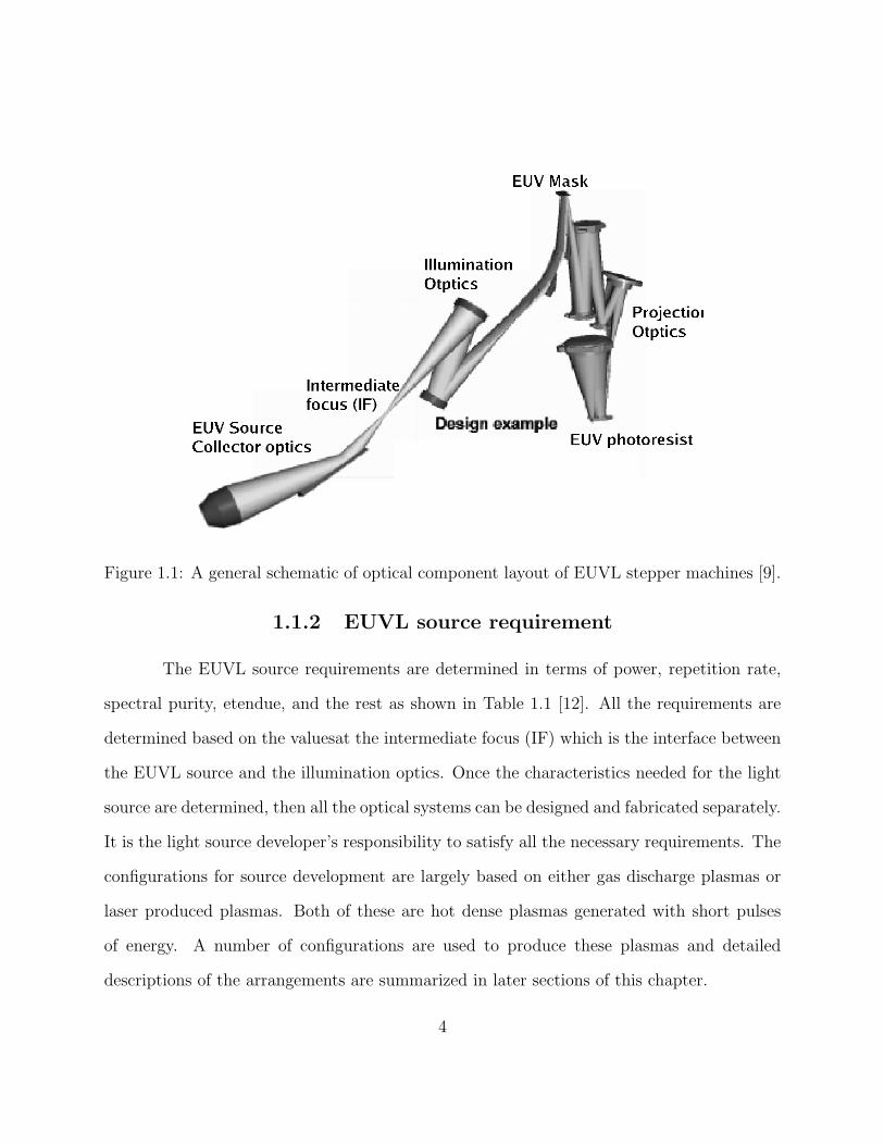
Figure 1.1: A general schematic of optical component layout of EUVL stepper machines [9].
1.1.2 EUVL source requirement
The EUVL source requirements are determined in terms of power, repetition rate,
spectral purity, etendue, and the rest as shown in Table 1.1 [12]. All the requirements are
determined based on the valuesat the intermediate focus (IF) which is the interface between
the EUVL source and the illumination optics. Once the characteristics needed for the light
source are determined, then all the optical systems can be designed and fabricated separately.
It is the light source developer’s responsibility to satisfy all the necessary requirements. The
configurations for source development are largely based on either gas discharge plasmas or
laser produced plasmas. Both of these are hot dense plasmas generated with short pulses
of energy. A number of configurations are used to produce these plasmas and detailed
descriptions of the arrangements are summarized in later sections of this chapter.
4

Table 1.1: Table 1 EUVL source requirements [12].
SOURCE CHRACTERISTICS REQUIREMENT·Wavelength 13.5 [nm]·EUV Power (in-band) 115 [W]∗
·Repetition Frequency > 7-10 kHz ∗∗∗
·Integrated Energy Stability ±0.3%, 3σ over 50 pulses·Source Cleanliness ≥ 30,000 hours ∗∗
·Etendue of Source Output max 3.3 mm2sr∗∗∗
·Max. solid angle input to illuminator 0.03 - 0.2 [sr] ∗∗∗
·Spectral Purity:130-400 [nm] (EUV/UV) ≤ 3-7% ∗∗∗
≥400 [nm](IRVis) at Wafer TBD ∗∗∗
∗ At IF
∗∗ After IF
∗∗∗ Design dependent
The most challenging areas to fulfill among the requirements listed are the inband
EUV source power and lifetime (listed as source cleanliness). To facilitate the continuous
operation of EUVL stepper machines, the light sources need to provide the required power
continuously with minimal interruptions, such as for routine maintenance (97% up-time).
The source power requirement depends on the desired product throughput, optical through-
put of the whole system, exposure field size, and photoresist sensitivity [13]. To achieve the
required light source power, the conversion efficiency (CE), the ratio of the energy supplied
relative to EUV energy generated in the narrow band, needs to be high. The CE value as
well as the source lifetime has been improved by many research groups in recent years.
1.1.3 Conversion efficiency
The conversion efficiency (CE) of useful EUV energy output from supplied input
energies is a very important factor in EUVL source development. It limits the maximum
5
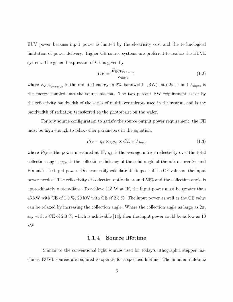
EUV power because input power is limited by the electricity cost and the technological
limitation of power delivery. Higher CE source systems are preferred to realize the EUVL
system. The general expression of CE is given by
CE =EEUV2%BW ·2π
Einput
(1.2)
where EEUV2%BW2πis the radiated energy in 2% bandwidth (BW) into 2π sr and Einput is
the energy coupled into the source plasma. The two percent BW requirement is set by
the reflectivity bandwidth of the series of multilayer mirrors used in the system, and is the
bandwidth of radiation transferred to the photoresist on the wafer.
For any source configuration to satisfy the source output power requirement, the CE
must be high enough to relax other parameters in the equation,
PIF = ηR × ηCol × CE × Pinput (1.3)
where PIF is the power measured at IF, ηR is the average mirror reflectivity over the total
collection angle, ηCol is the collection efficiency of the solid angle of the mirror over 2π and
Pinput is the input power. One can easily calculate the impact of the CE value on the input
power needed. The reflectivity of collection optics is around 50% and the collection angle is
approximately π steradians. To achieve 115 W at IF, the input power must be greater than
46 kW with CE of 1.0 %, 20 kW with CE of 2.3 %. The input power as well as the CE value
can be relaxed by increasing the collection angle. Where the collection angle as large as 2π,
say with a CE of 2.3 %, which is achievable [14], then the input power could be as low as 10
kW.
1.1.4 Source lifetime
Similar to the conventional light sources used for today’s lithographic stepper ma-
chines, EUVL sources are required to operate for a specified lifetime. The minimum lifetime
6

requirement is currently set at 30,000 hours, where a total number of source plasma gen-
erations is on the order of 1011 for the minimum repetition rate of 7 kHz. This minimum
repetition rate is set by the required dose stability, and is dependent on the source power
stability, assumed here to be < 1%. The collector mirror reflectivity is the only factor that
changes over time and is allowed to have a reduction of up to 10 % over the mirror lifetime
[15]. Reduction comes from the source plasmas emitting not only radiation but also ions
and particles of the target material that will degrade the reflectivity over time. It is a chal-
lenge to achieve long term plasma source operation without having any mirror reflectivity
degradation. The primary objective of the study reported in this thesis is to identify the
causes of the mirror degradation and to characterize the particulate debris and high energy
ion emissions. In addition, the prevention of the mirror degradation by mitigating the debris
and the ion emission will also be investigated.
1.2 EUV - Soft X-ray sources
The term ”EUV” is new, coming into use only during the last decade to describe the
wavelength range of light in the∼10 nm range. This is traditional called the Soft X-Ray range
(∼ 1 nm - 70 nm). However the lithography community preferred to use the term ”EUV” to
imply it being an extension of the current deep UV (DUV) methods (193 nm) currently now
in place. From an over-view perspective, EUV and soft X-ray radiation can be generated
either directly from transient motion of electrons or by the de-excitation of excited bound
electron in partially stripped ions. To generate an electromagnetic (EM) wave with short
wavelengths by the former mechanism, the acceleration of the electrons has to be large in
order to create a fast electric field transient. The radiation of synchrotrons, undulators, and
wigglers are based on the acceleration of the relativistic electrons. In the latter mechanism,
7
hot-dense plasmas are the sources of excited ions, existing in several ionization stages, that
gives rise to EUV or Soft X-ray emission. Gas discharge dense plasmas and laser produced
plasmas are generated easily in laboratories.
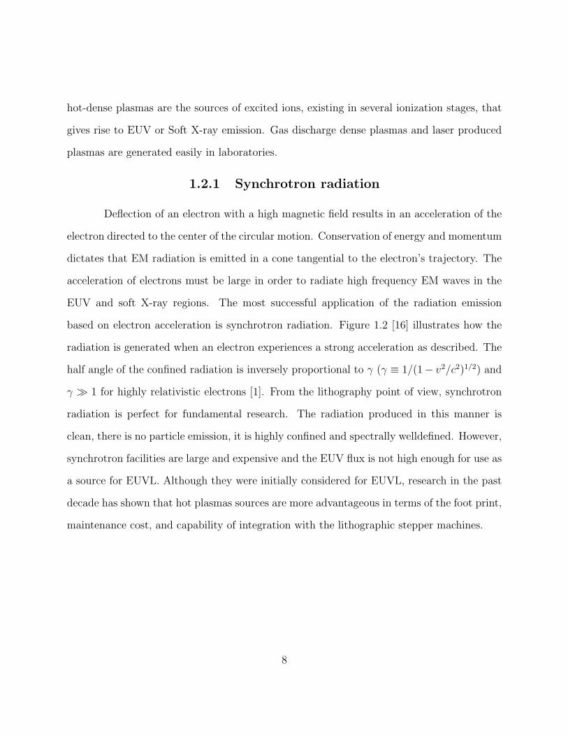
1.2.1 Synchrotron radiation
Deflection of an electron with a high magnetic field results in an acceleration of the
electron directed to the center of the circular motion. Conservation of energy and momentum
dictates that EM radiation is emitted in a cone tangential to the electron’s trajectory. The
acceleration of electrons must be large in order to radiate high frequency EM waves in the
EUV and soft X-ray regions. The most successful application of the radiation emission
based on electron acceleration is synchrotron radiation. Figure 1.2 [16] illustrates how the
radiation is generated when an electron experiences a strong acceleration as described. The
half angle of the confined radiation is inversely proportional to γ (γ ≡ 1/(1− v2/c2)1/2) and
γ 1 for highly relativistic electrons [1]. From the lithography point of view, synchrotron
radiation is perfect for fundamental research. The radiation produced in this manner is
clean, there is no particle emission, it is highly confined and spectrally welldefined. However,
synchrotron facilities are large and expensive and the EUV flux is not high enough for use as
a source for EUVL. Although they were initially considered for EUVL, research in the past
decade has shown that hot plasmas sources are more advantageous in terms of the foot print,
maintenance cost, and capability of integration with the lithographic stepper machines.
8

12γθ ~
Figure 1.2: Schematic of synchrotron radiation [16].
1.2.2 Gas discharge dense plasmas
There are two types of hot-dense plasma sources under development, laser plasma
sources and gas discharge sources. To attain radiation from plasmas predominately emitted
into the EUV regions, plasma temperatures of several tens of eV are required. The most
common gas discharge plasmas are created so-called ”pinch plasmas” between electrodes
with unique geometries where the discharge current confines the plasma itself and the pinch
confinement progressively increases the plasma temperature and density. The pinched plasma
subsequently collapses due to the growth of magneto-hydrodynamic instabilities.
Several different discharge configurations have been devised. Hollow cathode triggered
gas discharge [17],dense plasma focus plasmas [18], Z-pinch gas discharges [19], and capillary
discharges [20] are some of the typical configurations. A schematic of a gas discharge plasma
source configuration is shown in Figure 1.3 [21]. The debris generation process from gas
9
discharge plasmas is complex. The plasma as well as the electrodes can be the source of
debris. The lifetime of the electrode must be factored into the source lifetime, and the
electrode lifetime is one of the challenges gas discharge plasmas need to overcome.
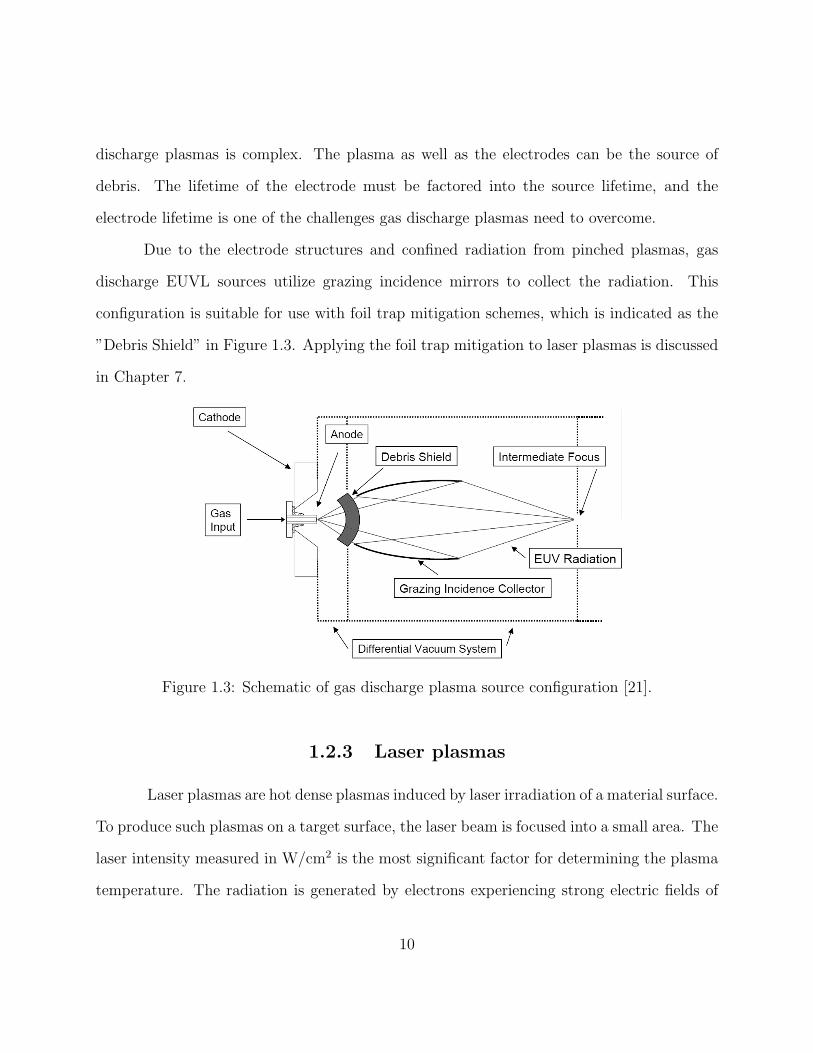
Due to the electrode structures and confined radiation from pinched plasmas, gas
discharge EUVL sources utilize grazing incidence mirrors to collect the radiation. This
configuration is suitable for use with foil trap mitigation schemes, which is indicated as the
”Debris Shield” in Figure 1.3. Applying the foil trap mitigation to laser plasmas is discussed
in Chapter 7.
Figure 1.3: Schematic of gas discharge plasma source configuration [21].
1.2.3 Laser plasmas
Laser plasmas are hot dense plasmas induced by laser irradiation of a material surface.
To produce such plasmas on a target surface, the laser beam is focused into a small area. The
laser intensity measured in W/cm2 is the most significant factor for determining the plasma
temperature. The radiation is generated by electrons experiencing strong electric fields of
10

ions (free-free emission) and also by the electrons de-excited in the energy levels in the
atoms and ions (bound-bound emission). There is no lifetime limitation on creating laser
plasmas if the target material is delivered continuously. The source lifetime of the EUV
light source is simply the lifetime of collector mirror reflectivity. A reduced mass target
can be used to reduce the debris generation in the plasma. Details of the laser and target
material configurations are discussed in Chapter 2. From the mitigation point of view, which
differs from gas discharge plasma sources, any mitigation schemes around the plasma block
the collected radiation. An example of a source, mirror and IF configuration for utilizing
laser plasma is shown in Figure 1.4 [22]. A suitable mitigation configuration is discussed in
Chapter 7.
Figure 1.4: An example of laser plasma EUV source, mirror, and IF configuration [22].
11

1.3 Multilayer mirror coating and reflectivity
The refractive indices of materials approach unity when the radiation wavelength
approaches EUV and soft x-rays. Refractive optics and reflective optics are very difficult to
be created for use with these wavelengths. Most materials absorb radiation at wavelengths
in the EUV and soft x-ray regions. However, multilayer coatings enable reasonably high
reflectivity at specific wavelengths by choosing the materials with small absorption at those
wavelengths. The general absorption properties of materials and the basic ideas of multilayer
mirrors are discussed in this section.
1.3.1 Absorption of soft X-ray in materials
The general form of the refractive index [1] as a function of the frequency of the
radiation is expressed in,
n(ω) = 1− δ + iβ (1.4)
where ω is the frequency of radiation that propagates in the material. The absorption decay
length (skin depth) is expressed by,
labs =λ
4πβ(1.5)
where labs is the distance until the electric field is reduced to 1/e. The expression shows
that the decay length is proportional to the wavelength and the absorption is based on the
complex component of refractive index. The complex component of the refractive index is
expressed with the atomic scattering factor.
β =nareλ
2
2πf 0
2 (ω) (1.6)
where na is atomic concentration of the material, re is the classical electron radius, and f 02
is the complex component of the atomic scattering factor. The atomic scattering factors of
12

most of the elements are found on the Center for X-Ray Optics (CXRO) website [23]. When
macroscopic characteristics of absorption are considered, absorption is expressed as,
I
I0
= e−ρµr (1.7)
where I is the intensity of incident wave measured at a distance of r from the surface, I0
is the intensity of the wave at the surface, ρ is the density of the material, and µ is the
absorption coefficient. The absorption coefficient is also expressed by the atomic scattering
factor,
µ =2reλ
Amu
f 02 (ω) (1.8)
where A is the atomic mass of the material, and mu is the unit atomic mass. The absorption
coefficient is proportional to the wavelength and the complex component of the atomic
scattering factor. There are rapid changes in the atomic scattering factors both of the real
and complex components as a function of wavelength [1, 23]. They are based on the resonance
of the bound electrons which differ from element to element. Therefore, the absorptions of
materials for short wavelength radiation are dependent on the nuclear structures in the
material atoms. In Chapter 3, more detailed absorption characteristics of thin films or thin
layers are described for materials that are important for the mirror reflectivity degradation.
1.3.2 Reflectivity of multi-layer mirror
The key to the high reflectivity of the multilayer mirror (MLM) is constructive wave
interference [1]. Typical multilayer coatings have a periodic structure of materials consisting
of a low Z material and a high Z material. The low Z materials are used just as spacers
where low absorption is expected. The high Z materials are used as absorbers where higher
absorption is expected. The high Z materials introduce a large difference in the refractive
index in the coatings. A cross section of multilayer mirror is shown in Figure 1.5 [24]. As
13

radiation is propagating in the coating, the wave is scattered at each layer having the large
refractive index. The wave propagation and scattering are constructively interfered when
the wavelength in the coatings satisfy the Bragg’s law,
mλ = 2d sin θ (1.9)
where m is an integer number, d is the thickness of the each period of the multilayer coatings,
and θ is the grazing angle of the wave.
Figure 1.5: TEM cross section image of Mo/Si multilayer mirror surface [24].
The reflective coating materials selected for EUVL are Si and Mo. Typical reflectivity
characteristics of a multilayer coating with Si and Mo is shown in Figure 1.6 [25]. The peak
reflectivity is about 0.7 and the bandwidth of the reflectivity is about 4% of 13.5 nm. Only
the radiation generated in the source plasma with the wavelength in the reflectivity band
is reflected. The rest of the radiation with wavelength outside the reflectivity band will be
absorbed by the mirror, resulting in mirror heating. The EUV mask is created on the multi-
layer mirror surface by depositing absorbing materials with the desired pattern [26]. There
are at least 6 multilayer mirrors in the projection optics before the EUV radiation reaches
14
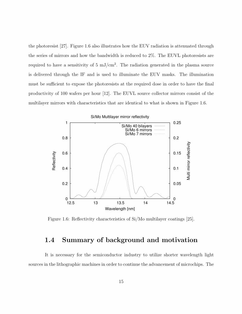
the photoresist [27]. Figure 1.6 also illustrates how the EUV radiation is attenuated through
the series of mirrors and how the bandwidth is reduced to 2%. The EUVL photoresists are
required to have a sensitivity of 5 mJ/cm2. The radiation generated in the plasma source
is delivered through the IF and is used to illuminate the EUV masks. The illumination
must be sufficient to expose the photoresists at the required dose in order to have the final
productivity of 100 wafers per hour [12]. The EUVL source collector mirrors consist of the
multilayer mirrors with characteristics that are identical to what is shown in Figure 1.6.
0
0.2
0.4
0.6
0.8
1
12.5 13 13.5 14 14.5 0
0.05
0.1
0.15
0.2
0.25
Ref
lect
ivity
Mul
ti m
irror
refle
ctiv
ity
Wavelength [nm]
Si/Mo Multilayer mirror reflectivity
Si/Mo 40 bilayersSi/Mo 6 mirrorsSi/Mo 7 mirrors
Figure 1.6: Reflectivity characteristics of Si/Mo multilayer coatings [25].
1.4 Summary of background and motivation
It is necessary for the semiconductor industry to utilize shorter wavelength light
sources in the lithographic machines in order to continue the advancement of microchips. The
15

most promising technique is EUVL, which utilizes a hot dense plasma source and multilayer
mirrors. The plasmas are generated using either gas discharges or lasers. The requirements
that need to be met by the light sources are challenging, especially in the areas of 1) EUV
power delivery and 2) the lifetime of the source and the collection optics. The EUV power
requirement is based on the photoresist sensitivity and the overall transmission of the series
of multilayer mirrors. The lifetime of the EUVL light source is determined by the lifetime
of the collector mirror reflectivity which is degraded by debris from the plasma.
The main mechanisms causing mirror reflectivity degradation are deposition and ero-
sion, which are discussed in Chapter 3. A common approach to reducing debris generation
and to extending mirror lifetime is to reduce the target mass. Even though the mass of the
target is reduced, collector mirror reflectivity degradation still occurs. The target material
can coat the mirror surface, leading to the absorption of EUV radiation. Energetic ions
created in the plasma can cause multilayer mirror surface sputtering as well. It is important
to characterize the mirror reflectivity degradation processes in order to identify the cause
and to prevent degradation, thus extending mirror lifetime. In this study target material
deposition processes, ion emission characteristics and debris mitigation are investigated. Fi-
nally, the potential of a laser plasma source to be realized as an EUVL source is discussed
in this study.
16

CHAPTER 2
LASER PLASMAS AND DEBRIS
2.1 Introduction
In this chapter, a description overview of laser plasma generation, debris generation,
and mass-limited target concepts including different target configurations are presented. The
laser plasma generation process involves the absorption of laser pulse energy, transitions in
the existing ionization stages, and thermal energy transfer to kinetic energy. During the
production of plasma on a solid surface different kinds of debris are also generated, each
posing a threat to the collection optics. The debris generation processes and different target
configurations are discussed in this chapter. There are many existing target configurations
that are designed to reduce debris generation. A common approach to minimize debris is
to reduce the mass of target. The ultimate goal of the approach is to realize a target where
the mass is limited to the minimum number of ions required for efficient radiation, which
is called the mass-limited target concept [28]. During the plasma generation process, while
utilizing a mass-limited target, the entire target is ionized. The knowledge of the number of
atoms in the target enables quantitative debris emission characteristics, which are discussed
in the later chapters. A short description of how to calculate the total number of atoms in
the target is also presented in this chapter.
17
2.1.1 Laser Plasma generation
Temperatures in laser plasmas typically exceed hundred thousand degrees Kelvin
which is equivalent to tens of eVs. (The plasma temperature is usually expressed in the unit
of eV where 1 eV is equal to 11604 K.) Simultaneously, the densities of these plasmas are
high since they are generated near the surfaces of solid. These plasmas have a large number
of multiply ionized ions which are the source for short wavelength radiation. The electron
transitions that have energy between the levels in such ions are typically tens of or hundreds
of eVs. The photons generated by electron transitions in these energy levels have energies
that correspond to the wavelengths in soft X-ray and EUV region. The laser pulse energy
is absorbed efficiently by the plasma in the region of high electron densities. Due to the
high electron density as a result the plasma expands rapidly and cools down. Most of the
thermal energy is transferred to kinetic energy. The ionization stages of ions are lowered by
recombination with electrons while the plasma is expanding.
2.1.2 Absorption of laser energy in fully ionized plasmas
The photon energy of a laser pulse is typically a few eV while the temperature of
plasma can exceed 10s of eVs. Laser plasmas can be heated by many processes involving
electrons, ions and photons. The leading absorption mechanism for an EUV source is called
three-body absorption or inverse Bremsstrahlung absorption which relies on the electrons
absorbing the laser light. The electron mass is much lighter than the ions in the plasmas
so the electrons can oscillate with the electric field in the laser pulse. When an electron ap-
proaches an ion, the electron experiences a Coulomb force. This force causes strong electron
acceleration due to the small mass of electron and the small distance between the electron
and ions. The electron radiates photons like that of synchrotron radiation but at an atomic
18

scale, which is referred as Bremsstrahlung radiation. The inverse of this process, where
a photon is absorbed by the collision process, is called inverse Bremsstrahlung absorption
(IBA).
The IBA process is the main absorption mechanism of a plasma when the laser inten-
sity is 1010 to 1012 W/cm2, and the interaction of the laser light is with a plasma scalelength
considerably longer than the light wavelength. The coefficient [29] of IBA is expressed in
K =16πZ2nenie
6lnΛ(ν)
3cν2(2πmekBT )3/2
1
(1− ν2p/ν
2)1/2(2.1)
where Z is the ionization state of ions, ne is electron density, ni is ion density, e is charge
unit, c is speed of light, ν is frequency of laser light, me is mass of electron, k is Boltzmann
constant, Te is electron temperature, νp is plasma frequency, and lnΛ = ln(vT /ωppmin) is
called the Coulomb Logarithm [30]. The plasma frequency is expressed as
νp =1
2πωp =
1
2π
√e2ne
ε0me
(2.2)
where ε is permittivity. pmin is the minimum impact parameter for electron and ion collisions
which is the maximum of either Ze2/kT or ~(mekT )1/2. The IBA coefficient is high when
the electron density is high and electron temperature is low. This ne, Te dependencies show
that the laser light is absorbed by the surface of the target at the beginning of plasma
generation. As a result of laser absorption creating high electron temperatures, the plasma
expands resulting in an electron density gradient on the front of the target. The newly
formed low density part of the plasma becomes transparent to the laser light allowing the
inner part of the plasma near the target to absorb the laser light. This laser light penetration
occurs progressively until all the laser energy is absorbed by the plasma or the laser light
encounters the plasma region whose frequency is equal to the laser light frequency. The
1/(1− ν2p/ν
2)1/2 term in Equation 2.1 causes the IBA coefficient to be infinite when the two
19

interacting frequencies are equal. In general, an EM wave is reflected by plasmas with a
plasma frequency higher than that of the incoming EM wave. This frequency is referred as
the electron plasma frequency, sometimes called the cut off frequency. For a specific laser
wavelength to be the cut-off frequency of the plasma, the electron density is obtained by
substituting the laser frequency in the plasma frequency in Equation 2.2. This electron
density is referred to as the critical density and for 1064 nm laser light is about 1021 els.
cm−3.
In addition to the IBA process, resonant absorption can occur at the critical density.
The process is resulting in strong local energy deposition and this causes hot (non-thermal,
collisionless) electron generation. The hot electrons can escape from the plasma once they
become out of phase with the resonant oscillation due to collisions with ions. The escaping
hot electrons will then drag nearby ions by Coulomb attraction these ions acquiring high
kinetic energies. This latter process is not likely to occur in the laser intensity region of this
study.
2.1.3 Ionization stages
The degree of ionization in the plasmas in this study is relatively high. For example
the tin ions will have about ten electrons stripped off at the plasma temperature of 30 eV
[31]. A tin atom has 50 electrons and the ionization potentials of tin ions range from about
7 eV to 300 eV until it becomes Kr like (Sn14+ ion). For lower Z materials, for instance,
lithium ions will have all the electrons except one stripped when the plasma temperature
reaches 10 eV [32]. The ionization stages are determined by the ionization potentials and
the electron temperatures.
With a plasma generated by IBA on a slow enough time-scale, (for the absorbed
20
energy to equilibrate in the plasma) it can be considered to be a thermalized plasma. Then
a maxwellian distribution can be used to describe the electron temperature. A higher tem-
perature of the distribution is sufficient to ionize the ions that the electrons collide with. It
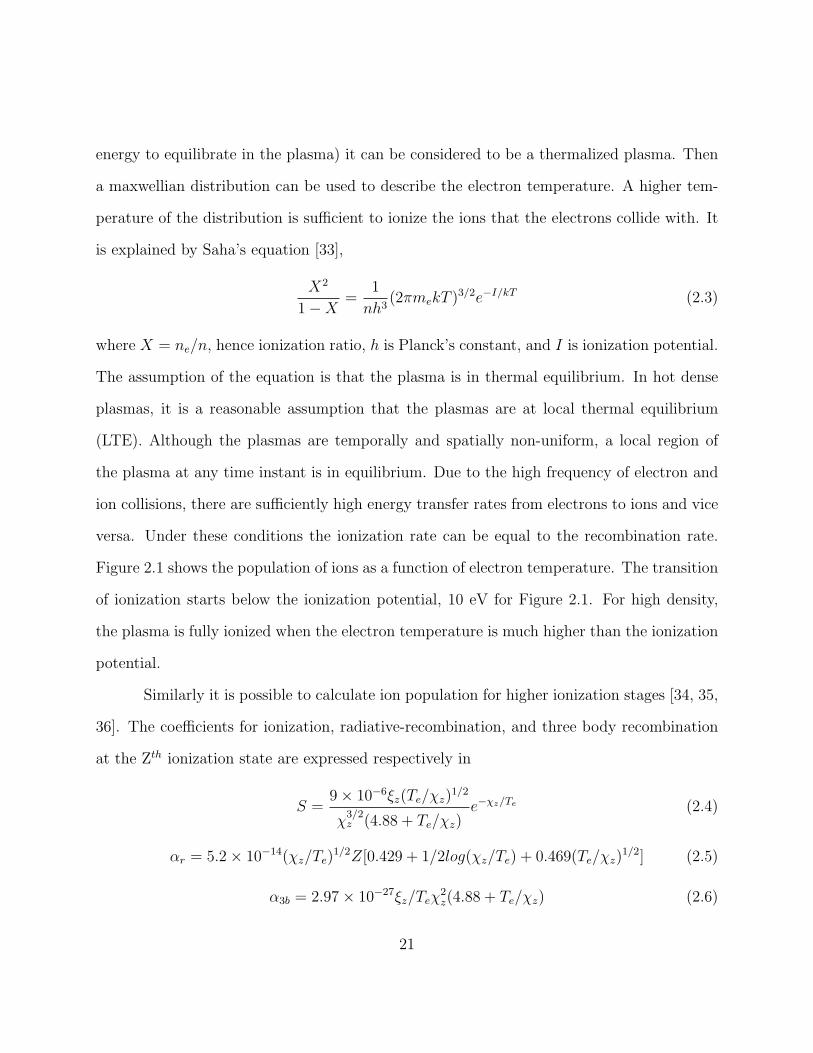
is explained by Saha’s equation [33],
X2
1−X=
1
nh3(2πmekT )3/2e−I/kT (2.3)
where X = ne/n, hence ionization ratio, h is Planck’s constant, and I is ionization potential.
The assumption of the equation is that the plasma is in thermal equilibrium. In hot dense
plasmas, it is a reasonable assumption that the plasmas are at local thermal equilibrium
(LTE). Although the plasmas are temporally and spatially non-uniform, a local region of
the plasma at any time instant is in equilibrium. Due to the high frequency of electron and
ion collisions, there are sufficiently high energy transfer rates from electrons to ions and vice
versa. Under these conditions the ionization rate can be equal to the recombination rate.
Figure 2.1 shows the population of ions as a function of electron temperature. The transition
of ionization starts below the ionization potential, 10 eV for Figure 2.1. For high density,
the plasma is fully ionized when the electron temperature is much higher than the ionization
potential.
Similarly it is possible to calculate ion population for higher ionization stages [34, 35,
36]. The coefficients for ionization, radiative-recombination, and three body recombination
at the Zth ionization state are expressed respectively in
S =9× 10⁻⁶ξz(Te/χz)
1/2
χ3/2z (4.88 + Te/χz)
e−χz/Te (2.4)
αr = 5.2× 10⁻¹⁴(χz/Te)1/2Z[0.429 + 1/2log(χz/Te) + 0.469(Te/χz)
1/2] (2.5)
α3b = 2.97× 10⁻²⁷ξz/Teχ2z(4.88 + Te/χz) (2.6)
21

0
0.2
0.4
0.6
0.8
1
0.1 1 10 100
Ioni
zatio
n ra
tio
Electron temperature [eV]
ne=1022 [cm-3]ne=1018 [cm-3]ne=1014 [cm-3]
Figure 2.1: Ionization rate calculation at different electron densities.
where z is the ionization stage, ξZ is the number of electron in the most outer orbit of the
stage, and χZ is the ionization potential. Radiative Recombination is a process where an
electron is captured by an ion and recombines into an excited level. Then the electron makes
a radiative transition to a lower level. The Three Body Recombination process is one in
which an electron is captured by an ion and the excess energy of the electron is sufficient
to excite another electron. The excited electron eventually decays down to a lower energy
state of the ion with consequential emission of radiation. The electron density rate at the
Zth ionization state is given by the equation [36]
dnz+1
dt= nenzS(z, Te)− nenz+1[S(z + 1, Te) + αr(z + 1, Te) + neα3b(z + 1, Te)]
+ nenz+2[αr(z + 2, Te) + neα3b(z + 2, Te)] (2.7)
When a stationary state is assumed, the ratio of two adjacent ionization stages in equilibrium
22

is expressed in,
nz+1
nz
=S(z, Te)
αr(z + 1, Te) + neα3b(z + 1, Te)(2.8)
For high Z materials like tin, some of the ionization potentials are so close that several
ionization stages exist at the same electron temperature [37]. Figure 2.2 illustrates ion
population for different electron temperatures for the case of tin plasma with the electron
density of 1021 cm−3. The ionization potentials used in the calculation for the different tin
ions are found in the literatures [38, 39].
Figure 2.2: Population of tin ion species as function of electron temperature.
2.1.4 Fluid descriptions of laser plasmas
There are a number of ways to describe plasmas mathematically. For example, a
fluid expression that describes the temperature, pressure, and motion of the fluid in terms
of hydrodynamics or fluid-dynamics can be applied. If as assumed previously, the electron
23

energy distribution is Maxwellian, the electron temperature is expressed by only one value.
Similarly, temperature values can be expressed for other species as well. A set of (mixture
of) multiple fluids is typically used to describe fluid characteristics of plasma. Typically,
electrons and ions are the two interacting fluid species described.
There are three sets of equations [1, 40, 41] for each fluid species that are used to
calculate the motion of fluid at different times. The electron temperature and density are
typically calculated progressively along with instantaneous laser pulse energy. In this study,
two different simulation codes are utilized which are discussed in Chapter 6.
Conservation of particle number is expressed in,
∂n
∂t= −∇ · (n~v) (2.9)
where n is the density of a species and v is the average velocity. Conservation of momentum
is expressed in,
nm∂~v
∂t= −∇P + nq( ~E + ~v × ~B)− ~Ffric (2.10)
where m is the mass of the species, P is the pressure, q is the charge of the species, E is
electric field, B is magnetic field and Ffric is the friction force caused by collisions with other
species. Conservation of energy is expressed in,
n∂U
∂t= −P∇ · ~v +
∂Utrans
∂t+
∂Udep
∂t(2.11)
where U is the thermal energy, Utrans is the transferred energy due to collisions with other
speices, and Udep is the energy deposited in the plasma. For the laser plasma case, Udep is
absorbed laser energy. The friction force term in Equation 2.10 is expressed in
~Ffric =∑
j
αaj(~va − ~vj) (2.12)
24

for multi species case. The coefficient is expressed in each species pair
αab = nanbmabα′ab (2.13)
where mab = mamb/(ma +mb) is reduced mass from each mass of species. The coefficient α′
[40] of friction force is expressed in,
α′ab =
4√
2πZaZbe4lnΛ
3√
mab(kT )3/2(2.14)
which is the collision frequency of two species.
The energy transfer term of the Equation 2.11 is a result of collisions between two
different species where a temperature is higher than the other.
∂Utrans
∂t=
∑j
3
2naα
′ajk(Tj − Ta) (2.15)
Based on these equations, a laser plasma is described from the beginning of the laser pulse,
to the end when the plasma reaches the collector mirror after expansion. A simplified
simulation model that utilizes these equations is constructed and the details of the simulation
are described in chapter 6.
2.1.5 Plasma expansion
Plasma generated by a nanosecond Gaussian laser pulse starts to expand rapidly well
before the laser power reaches the peak. The pressure gradient will accelerate the motion of
plasma as described in Equation 2.10. Such expanding plasma is rapidly cooled down. As
seen in Equation 2.11, decompression due to velocity divergence reduces the temperature if
there is no energy addition. There is no mechanism to increase the ionization stages while
the temperature is decreasing. The ionization stages will be reduced through recombination
processes.
25
2.1.6 Recombination
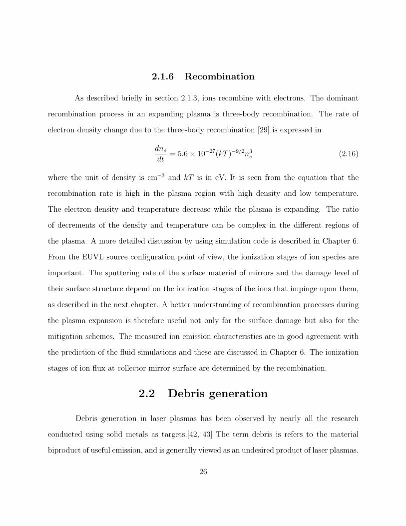
As described briefly in section 2.1.3, ions recombine with electrons. The dominant
recombination process in an expanding plasma is three-body recombination. The rate of
electron density change due to the three-body recombination [29] is expressed in
dne
dt= 5.6× 10⁻²⁷(kT )−9/2n3
e (2.16)
where the unit of density is cm−3 and kT is in eV. It is seen from the equation that the
recombination rate is high in the plasma region with high density and low temperature.
The electron density and temperature decrease while the plasma is expanding. The ratio
of decrements of the density and temperature can be complex in the different regions of
the plasma. A more detailed discussion by using simulation code is described in Chapter 6.
From the EUVL source configuration point of view, the ionization stages of ion species are
important. The sputtering rate of the surface material of mirrors and the damage level of
their surface structure depend on the ionization stages of the ions that impinge upon them,
as described in the next chapter. A better understanding of recombination processes during
the plasma expansion is therefore useful not only for the surface damage but also for the
mitigation schemes. The measured ion emission characteristics are in good agreement with
the prediction of the fluid simulations and these are discussed in Chapter 6. The ionization
stages of ion flux at collector mirror surface are determined by the recombination.
2.2 Debris generation
Debris generation in laser plasmas has been observed by nearly all the research
conducted using solid metals as targets.[42, 43] The term debris is refers to the material
biproduct of useful emission, and is generally viewed as an undesired product of laser plasmas.
26
There are research fields where debris generation is useful. Pulsed laser deposition (PLD) is
one of the largest research areas that use debris. In the PLD process, a laser beam ablates
the target material and the ablated material is deposited on a substrate. PLD is a fast
process, and it is possible to deposit compositions of targets which are preserved in the laser
ablation [44]. These are the advantages of PLD over other deposition processes. As is seen
in PLD, the focused laser beam creates not only plasma but also molecules, clusters, and
larger size liquid/solid pieces that are not decomposed by the laser beam. In research areas
such as EUVL, these material emissions are identified as debris.
2.2.1 Solid target and debris
When the laser beam is focused on the cold surface of a solid target, the temperature
of that area increases rapidly. This rapid temperature increase causes thermal expansion
of the material. The expansion occurs locally in the focal region and the material outside
the focus is still cold. When the propagation of the high pressure region is faster than the
heat transfer, the cold material at the boundary suffers severe damage such as cracks. When
the material surfaces are cracked to small pieces and their kinetic energies are high enough
to eject out of the surface, they become hot rocks and emanate from the target surface.
The material portions that are heated high enough to become liquid phase will break up
into aerosols (smaller droplets). To distinguish these droplet from the droplet target, in this
thesis ”Arosols” is used to express these small droplets. The liquid starts to expand and eject
from the target surface due to the pressure gradient near the target surface. The aerosols
also fly out into the environment.
Hot rocks and aerosols can be created without plasma generation. Ions, neutral atoms,
radicals, and electrons are created during plasma generation when the laser irradiation is high
27

enough to produce plasma. The energy coupled into the plasma generation is transferred
to the kinetic energies of ions, electrons, neutral atoms, radicals or molecules. As shown in
Chapter 6, the ion emission can be lethal to the multilayer mirror surface.
Laser plasmas produced from a solid target will generate all varieties of material
emission as mentioned above. This debris generation is one of the limitations in using laser
plasmas for industrial applications. Due to debris issues, the preferred material in the early
stage of EUVL source research was gaseous xenon. Xenon targets are believed to be debris
free because it is inert gas and does not generate any hot rocks or aerosols.
2.2.2 Hot rocks and aerosols
Hot rocks and aerosols were observed early on in EUVL source development [45, 46].
Characterizations of debris, in terms of size, shape, velocity, and emission distributions were
investigated and ideas for debris mitigation were discussed. The large sizes of particles are
the most threatening factor causing damage to the x-ray optics near the source. The particles
can be in solid and liquid phase. A perfect example describing the impact on the multilayer
mirror surfaces introduced by hot rocks and aerosols are obtained from Li planar target and
Sn planar targets [47]. Figure 2.3 shows optical microscope images, 3D profiler images, and
the cross sections of the profiles of multilayer mirror surfaces for both Li and Sn targets.
Microscope images show a number of material particulates on the mirror surfaces. The 3D
profiler images show a more detailed view of the surface damage. The debris generated
from the Li plasma shatters the multilayer mirror surface, a consequence of the flying by
hot rocks. In contrast, the debris generated by Sn plasmas is seen to create deposits on
the sample surface as a result of flying aerosols. Surface damage caused by hot rocks from
Sn plasma is also observed. Both types of damage degrade the mirror reflectivity despite
28

the differences in the degradation process. The generation of hot rocks and aerosols can be
eliminated by applying the mass-limited target concept which is described in a later section.
The degradation processes are described in more detail in Chapter 3.
Figure 2.3: Comparison of multilayer mirror surfaces exposed by Li and Sn plasmas [47].
2.2.3 Ions, electrons, and neutral atoms
Because the plasmas are generated by the laser pulse, there are always ions and
electrons present. Due to the small mass of electrons, the damage caused by electron flux
is negligible. Depending on the mass of ion species, ion incidents can cause severe damage
to the multilayer structure. The damage appears as erosion of the mirror surface over the
number of plasma generations. There are neutral atoms depending on the ionization ratio of
the plasma and on the recombination processes after the plasma generation. A neutral atom
of the target material has the same mass as the ions of the material. Thus the damage caused
by neutral atoms is similar to the damage caused by ions. The degradation process caused
29

by ions is discussed in Chapter 3 and the measurement of ion flux and energy distributions
is discussed in Chapter 6.
2.3 Mass-limited target
Debris free laser plasma sources are realized by reducing the emission of the hot
rocks and aerosols to a minimum. The first step to reduce the debris from the laser plasmas
is to utilize reduced mass of the target. The EUVL source development trend is reducing
the mass of the target and varying in different target materials, compounds, geometries, and
the way to supply the targets to the laser focus. However, at the same time the radiation
in the useful band is required to be high enough to be a useful light source. The only
target configuration that provides both the minimum debris and the maximum radiation is
the mass-limited target [28, 48]. The mass-limited target contains just sufficient number of
radiator atoms and the entire target is ionized up to the desired plasma temperature for
the required radiation. As the results of the complete ionization, there are no hot rocks
or aerosols generated. The target configuration trend in the EUVL source developments is
described.
2.3.1 Different target configurations
There are a number of compositions and geometries for target delivery in the EUVL
source development field in order to realize the reduced mass targets. They can be catego-
rized into three types; Xe targets, liquid metal targets, and tin doped targets. Xenon targets
are one of the candidate materials for the EUVL source. Xenon is in gas phase at room
temperature so that the target material does not deposit or block the EUV radiation on the
multilayer surface. However, Xe in gas phase does not have high enough atomic concentra-
30
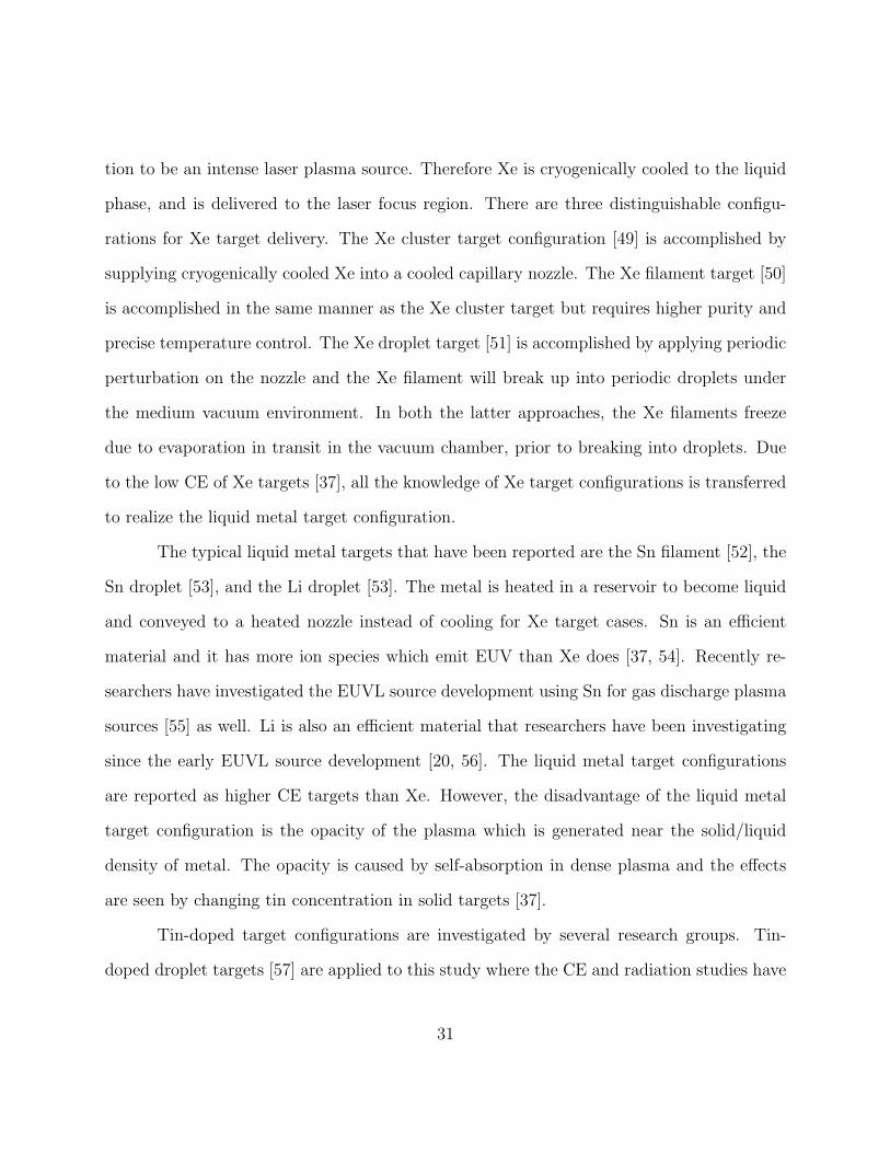
tion to be an intense laser plasma source. Therefore Xe is cryogenically cooled to the liquid
phase, and is delivered to the laser focus region. There are three distinguishable configu-
rations for Xe target delivery. The Xe cluster target configuration [49] is accomplished by
supplying cryogenically cooled Xe into a cooled capillary nozzle. The Xe filament target [50]
is accomplished in the same manner as the Xe cluster target but requires higher purity and
precise temperature control. The Xe droplet target [51] is accomplished by applying periodic
perturbation on the nozzle and the Xe filament will break up into periodic droplets under
the medium vacuum environment. In both the latter approaches, the Xe filaments freeze
due to evaporation in transit in the vacuum chamber, prior to breaking into droplets. Due
to the low CE of Xe targets [37], all the knowledge of Xe target configurations is transferred
to realize the liquid metal target configuration.
The typical liquid metal targets that have been reported are the Sn filament [52], the
Sn droplet [53], and the Li droplet [53]. The metal is heated in a reservoir to become liquid
and conveyed to a heated nozzle instead of cooling for Xe target cases. Sn is an efficient
material and it has more ion species which emit EUV than Xe does [37, 54]. Recently re-
searchers have investigated the EUVL source development using Sn for gas discharge plasma
sources [55] as well. Li is also an efficient material that researchers have been investigating
since the early EUVL source development [20, 56]. The liquid metal target configurations
are reported as higher CE targets than Xe. However, the disadvantage of the liquid metal
target configuration is the opacity of the plasma which is generated near the solid/liquid
density of metal. The opacity is caused by self-absorption in dense plasma and the effects
are seen by changing tin concentration in solid targets [37].
Tin-doped target configurations are investigated by several research groups. Tin-
doped droplet targets [57] are applied to this study where the CE and radiation studies have
31

been conducted by previous and current colleagues [58, 59]. The tin-doped target is the
only masslimited target configuration and realized by making droplets with SnCl2 solution.
Another target configuration in which tin is chemically doped is SnO2 cell targets [60]. The
tin particle can be doped into the target [57] and being developed by mixing tin particles
into water and making droplets containing these tin particles [61]. These tin doped target
configurations reduce not only the total mass of the target but also the mass of tin in the
target. A small mass of tin reduces the debris generation which is important in utilizing
this metal for EUVL sources. Similar reductions are expected by reducing the density of
metal targets. The density can be reduced by ablating solid or liquid metal targets before the
heating laser pulse is focused on the target. One common method to reduce the target density
is to use pre-pulse [62]. However, the larger part of the target materials remains at the solid
density and it is not producing any EUV radiation. This unused target material is wasted
and moreover can generate the hot rocks and aerosols. Thus for all the target configurations,
controlling the target mass is an important factor to reduce debris generation.
2.3.2 Number of atoms in a target
As described previously, the EUVL source development trend is utilizing the reduced
mass of the target, where the number of atoms that produce the EUV radiation is unknown.
In contrast, counting the number of atoms in the target is possible once the mass-limited
target is realized because all of the materials are consumed in producing the plasma With the
knowledge of the number of atoms in the target, it is possible to analyze debris quantitatively
and the analyses are described in Chapter 5 through 7. The number of atoms in a specific
target can be calculated with some reasonable assumptions and approximations. For the
droplet targets in this study, one important assumption is that the size of each individual
32

droplet is equal to all the droplets generated. This is a reasonable assumption when the
droplets are created by a capillary nozzle with stable stimulation at a constant frequency
[63] as the target material breaks into uniform size droplets that are equally spaced.
There are several ways to determine the size or mass of the target. Microscopy of
the target using a short-pulse back-illumination at a given magnification and resolution
determines the diameter of the target. To obtain the number of atoms in the target, it
is necessary to know the density of the target material and the mass concentration of the
target composition. Another way is to calculate the size of the droplet. The flow rate of the
material is determined by measuring the outer diameter of the material jet, and velocity of
the target. The volume of the target is calculated by the flow rate and the frequency of the
stimulation. The velocity is obtained by measuring the spacing between adjacent droplets
and the period of the stimulation. The density of the target has to be known as well. The
easiest way to measure the mass flow rate is to capture the target materials ejected in a small
container in a given time duration. This method provides the mass of the target directly
by dividing the mass flow by the frequency. The density of the target does not have to be
known to count the number of target atoms.
The number of atoms in the target for this study is calculated as follows. The cap-
tured mass of the target per minute is 1.0 x 10⁻¹ g and by dividing the total number of
target generation of 6.0 x 10⁶ (100 kHz), the mass of a single droplet is found to be 1.7
x 10−8 g. The fractional mass of all the elements in the target solution are in the ratio
H:O:Cl:Sn=0.06:0.49:0.17:0.28. The mass of tin in the target droplet is 4.8 x 10⁻⁹ g where
the mass of a single tin atom is 2.0 x 10⁻²⁵ kg. Therefore the number of tin atoms in the
target droplet is 2.4 x 10¹³. In addition, the number of tin atoms decreases or increases
as the driving frequency changes. The number of tin atoms can therefore be scaled by the
33

driving frequency. The typical frequencies for this study are 30 kHz, 50 kHz and 100 kHz.
Thus the numbers of tin atoms used are 4.8 x 10¹³ and 7.2 x 10¹³ for 50 kHz and 30 kHz
respectively.
2.4 Summary of laser plasmas and debris generation
Typical machanism of laser plasmas which are generated with laser intensities of 1010
to 1012 are IBA, characteritcs of high ionization stages, rapid plasma expansion, and three
body recombination. A fluid description of plasma can be used to express how the plasma
expands and how the plasma parameters change at different times. The generation of debris
from laser plasmas on solid targets is lethal to the collector mirror surfaces. Different types
of target configurations that utilize reduced mass of the target are being investigated for
EUVL source development. However, only the mass-limited enables comparison between
the number of atoms in the target and debris emission and flux at the collector mirror
surfaces.
34

CHAPTER 3
MULTILAYER MIRROR REFLECTIVITY
DEGRADATION
3.1 Introduction
As described in Chapter 1, the lifetime of the EUV light source is evaluated at the
intermediate focus (IF). To deliver the required EUV power to the IF, the collection optics
is considered a part of the EUV light source. For droplet plasma source the reflectivity of
the collector mirror is based on normal incident multilayer mirror structures. Any absorbing
materials on the top of the multilayer coatings caused by deposition and oxidation will reduce
the reflectivity and thus the source lifetime. Any structural degradation of the multilayer
coatings caused by surface sputtering, observed as erosion, can also reduce the reflectivity,
and hence the lifetime. This chapter discusses the reflectivity degradation processes and
impacts of deposition, oxidation and erosion on the multilayer coatings.
3.2 Deposition
As described in Chapter 1, the periodic structure of Si/Mo layers is the key to
achieving high reflectivity at 13.5 nm. In this chapter the processes that will degrade the
mirror reflectivity are considered. Once the periodic structure is destroyed the mirror reflec-
tivity drops precipitously. Any absorbing materials on the mirror surface will degrade the
reflectivity as well, even if the mirror structure maintains high reflectivity characteristics.
As discussed in Chapter 2, the debris generated from laser plasmas can destroy the multi-
35

layer coatings. These debris emissions from the plasmas are the most threatening factor for
the multilayer coatings. Also discussed is how the laser plasma based on the mass-limited
target concept can eliminate incident of particulates of target materials. However, since
the plasmas are generated in vacuum, the target material emanates as the plasmas expand.
Depending on the ion kinetic energies, typically smaller than 100 eV [64, 65], the metallic
ions are deposited on the multilayer mirror surfaces. The target materials that deposited
cause mirror reflectivity degradation. In this section, the absorption of a thin film of target
material is discussed.
3.2.1 EUV absorption of target materials
Most materials used as laser plasma target materials absorb EUV radiation due to
the fact that since the radiation is generated by electron transitions in the ions, it can be
absorbed by other electron transitions in other ions and atoms. Figure 3.1 illustrates the
absorption coefficients for possible target materials, Li, Sn, and Xe. The characteristics are
calculated by using Equation 1.8 and the f 02 values are referenced from the Center for X-Ray
Optics (CXRO) website [23]. All the target materials have absorbing properties for EUV
radiation with photon energies of approximately 90 eV. The unit of the absorption coefficient
is cm2/g. Li is a much lighter element than Sn so for a given volume or given thickness of
these two materials, Li has less absorbing properties as can be seen from Equation 1.7. Xe
is in a gas phase at room temperature so that EUV radiation absorbed by Xe gas is smaller
than that by Li and Sn. However, a much larger effort is required to pump Xe gas out of
the source chamber since it is much heavier than air. If cooled liquid Xe is continuously
supplied in the chamber without having high enough vacuum pumping power, the number
of Xe atoms in the source chamber will increases. The density of Xe gas is lower than that
36

in the solid or liquid phase. However, the absorption is not negligible because the radiation
experiences a longer path in the Xe filled environment. For any of these target material it is
important to remove the target atoms in the optical path of the EUV radiation.
100
1000
10000
100000
10 100 1000
µ [c
m2 /g
]
Photon energy [eV]
Absorption coefficient
LiSnXe
Figure 3.1: Absorption coefficient of Li, Sn, and Xe.
3.2.2 Absorption estimates of thin film
When target materials are deposited on the multilayer mirror surface, the mirror
reflectivity drops due to absorption in the film. The reduction factor depends on the thickness
of the deposition and its coverage area on the surface. Usually the multilayer structures are
preserved under the deposition unless the deposition layer diffuses into or reacts chemically
with the multilayer structures. As described in the previous section, the EUV radiation
absorbed by the target atoms can be estimated from known atomic scattering factors, and the
density of the materials. Figure 3.2 compares the transmission of thin films made of Si, Nb,
37

Ru, Li, and Sn. The transmission characteristics of Si, Nb, and Ru are shown as references
since they are commonly used as capping layers for multilayer mirror coatings [66]. The
materials for the capping layer are chosen for their low absorption of EUV radiation and their
high chemical stability in preventing oxidation and carbonization. Thus the transmissions
of those materials are required to be high. The transmission curves are obtained by the
calculation program available on the CXRO website [25]. The transmission of Sn thin film
is significantly lower compared to other materials.
0.4
0.5
0.6
0.7
0.8
0.9
1
12.5 13 13.5 14 14.5 15
Tran
smis
sion
Wavelength [nm]
Figure 3.2: Transmission of thin film 10 nm of Si, Nb, Ru, Li, and Sn [25].
Si
LiNb
Ru
Sn
The EUVL stepper roadmap requirements stipulate that the transmission of the de-
position layer can cause no more than a 10% reduction in the reflectivity at the end of the
mirror lifetime. This sets the maximum thickness of the depositing layer. The latter must
be reduced to half this value because the double path of the radiation on the mirror surface
must be considered. As can be seen, the maximum thickness of deposited thin layer of Li
38

can be up to 5 nm. The transmission of a Sn thin film with 1.5 nm thickness is close to
90%. Thus the maximum thickness for Sn deposition is only 0.75 nm to provide a < 10%
reduction factor.
3.2.3 Oxidation of multi-layer mirror surfaces
Oxidation of the multi-layer mirror surface has a similar effect on the reflectivity
degradation to the degradation as that caused by deposition. Oxygen is a strong absorber
of EUV which makes oxides so detrimental. Usually oxidation occurs at the interface of
the multilayer coatings to the vacuum environment, however, the oxidation process is rather
complex. In addition, once the silicon surface is oxidized, it is very difficult to remove the
oxidized layer. To prevent the oxidation of Si a so-called ”Capping layer” is deposited on the
Si surface. More research on oxidation has been reported in the area of the projection optics
than on the collection optics as the impact of oxidation of the mirror to the projection optics
is more significant than that to the collection optics. Researchers are currently investigating
the oxidation processes [67], reducing the oxidation rate [68], and removing the oxidation
from the capping layers [69]. In this section the impacts of absorption from the oxide layers
on the collector mirror optics are discussed.
3.2.4 Absorption of an oxide layers
A similar calculation of the EUV absorption characteristics of thin films described in
the previous section is carried out for the case of oxide layers. Figure 3.3 shows an example
of the transmission of SiO and SiO2 layers as compared to a Si layer with the same thickness.
The EUV absorption caused by oxygen atoms is dominant for oxide layers due to the high
transmission of Si. A thickness of 10 nm is just sufficient to keep the reflectivity within the
lifetime requirement of 10% reflectivity degradation. This is equivalent to oxidation of only
39

a half of the top Si layer of the multilayer structure, assuming uniform oxidation. Because of
the process, a SiO2 layer thickness of approximately 5 nm results when a Si layer thickness
of about 2.4 nm is oxidized. If the entire Si top layer is oxidized, the reflectivity drops more
than the requirement. Therefore oxidation has to be minimized as much as possible.
0.75
0.8
0.85
0.9
0.95
1
10 11 12 13 14 15 16
Tran
smis
sion
Wavelength [nm]
Figure 3.3: Transmission of oxide layers [25].
Si
SiO
SiO2
3.2.5 Photon induced oxidation processes
The oxidation process of the multilayer coating is a complex process. Several re-
searchers have reported that the process involves EUV radiation. The first result, which
is reported from the engineering test stand [70] (ETS), indicates that the oxidation rate is
significantly higher under EUV radiation exposure [69]. Another study has reported that
the oxidation process is a function of EUV dose, EUV intensity, and residual pressures of
oxygen or water vapor [67]. The EUV dose is measured in J/mm2, and the EUV irradiance
40

is measured in W/mm2. Some research reports that just the residual water pressure is not
the key for oxidation of a Ru capping layer [71]. The presence of hydrocarbons influences
the oxidation processes as well. Other researchers report on reducing the oxidation rate with
hydrocarbons [72], on modeling the oxidation processes [73] and removing oxidation layer
from Ru capping layer with use of hydrogen [70].
3.2.6 Impact on oxidation on collector mirror surfaces
The impact of oxidation on the collection optics is discussed in the previous section.
Although the relationship between water pressure and the oxidation rate is not simple, the
tendency for oxidation can be used to estimate the reflectivity lifetime of the mirror. Figure
3.4 shows the mirror reflectivity degradation as a function of EUV dose, and the degradation
slope as a function of EUV intensity [67]. The reflectivity drop is measured under water
pressure of 1 x 10⁻⁴ Pa. The degradation slope is linear with respect to the EUV intensity.
The experimental condition is approximately 10 mW/mm2, which is typical for the projection
optics. The EUV irradiance at the collection optics is around 1 mW/mm2 which is one order
of magnitude lower than that in the projection optics. The irradiance is based on uniform
illumination of the mirror, the mirror distance from the plasma source of 20 cm, and the
source power of 300 W in 2% 2π sr. By extrapolating the slope characteristics in Figure
3.4, the slope of 1 x10⁻⁵ mm2/J can be obtained at the EUV irradiance of 1 mW/mm2. For
10% reflectivity reduction, a dose of 104 J/mm2 is required. At the irradiance of 1mW/mm2,
the lifetime is about 107 s, which is equivalent to 3,000 hours. It is one order of magnitude
shorter than the lifetime requirement. This indicates the possible threat to oxidation of the
collection optics.
41
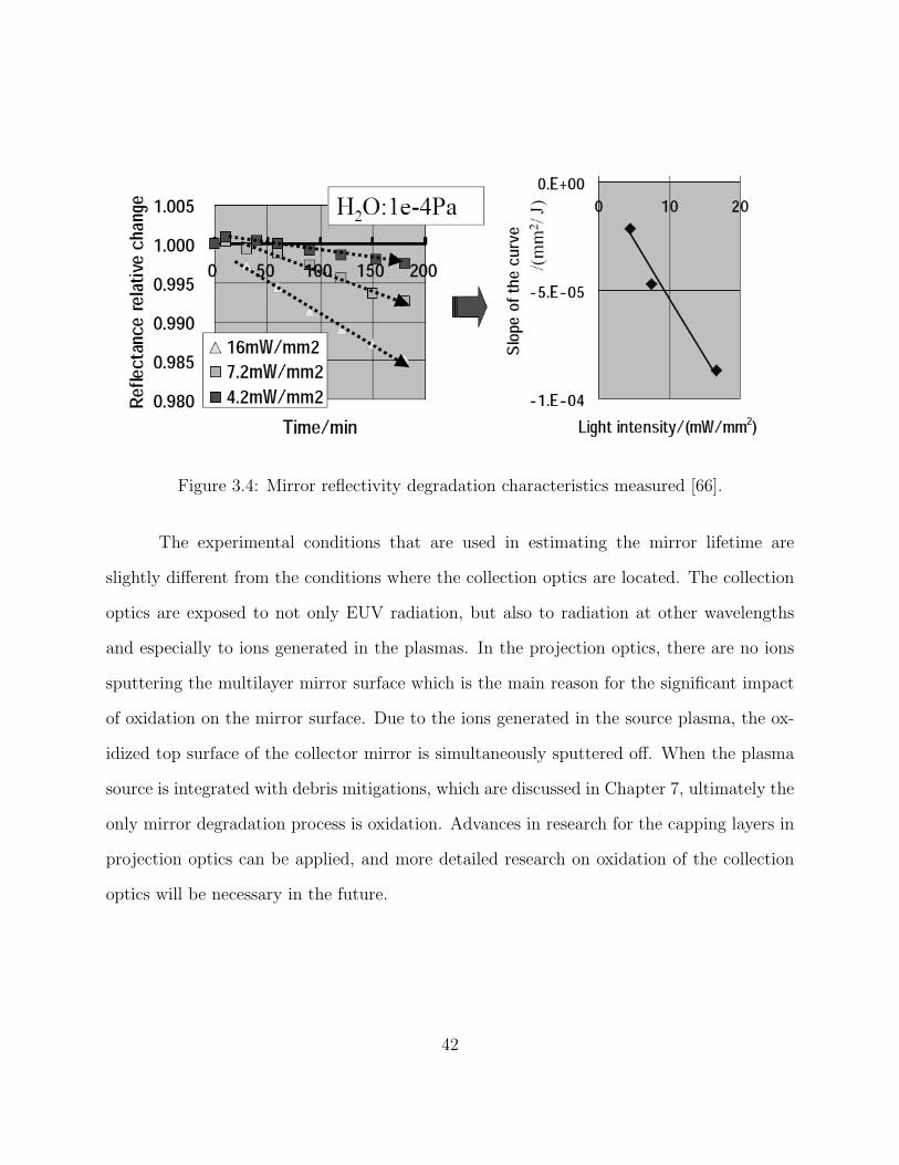
Figure 3.4: Mirror reflectivity degradation characteristics measured [66].
The experimental conditions that are used in estimating the mirror lifetime are
slightly different from the conditions where the collection optics are located. The collection
optics are exposed to not only EUV radiation, but also to radiation at other wavelengths
and especially to ions generated in the plasmas. In the projection optics, there are no ions
sputtering the multilayer mirror surface which is the main reason for the significant impact
of oxidation on the mirror surface. Due to the ions generated in the source plasma, the ox-
idized top surface of the collector mirror is simultaneously sputtered off. When the plasma
source is integrated with debris mitigations, which are discussed in Chapter 7, ultimately the
only mirror degradation process is oxidation. Advances in research for the capping layers in
projection optics can be applied, and more detailed research on oxidation of the collection
optics will be necessary in the future.
42
3.3 Erosion on multi-layer surfaces
The erosion of the multilayer mirror collection optics is caused by high kinetic energy
ions sputtering off the surface atoms as described in Chapter 2. Besides oxidation of the
multilayer mirror found in ETS, erosion is also observed at the collection optics surfaces
[74] The ETS collector mirror reflectivity degradation indicated that some 15 bi-layers were
removed over 5 x 10⁸ plasma generations for the EUV source conditions used. This source
utilized the Xe cluster target. A follow-up experiment on ETS suggested high energy ions
with kinetic energies up to 60 keV [75]. However, the evidence for these high energy ions
was not completely confirmed, and if evident, may well have been a consequence of using
the Xe cluster target.
Another multilayer mirror erosion study was carried out using water droplet target
[76]. The target geometry and the laser intensities for the water droplet target were equiva-
lent to the conditions applied to this study. The mirror erosion was found to be caused by
the high energy oxygen ions, which is shown in Figure 3.5. The erosion is an accumulated
result of extensive sputtering caused by high energy ions generated by each plasma event.
Therefore, understanding the sputtering characteristics of materials used in the multilayer
coatings, as well as the ion kinetic energy distributions, are very important for the erosion
studies.
43
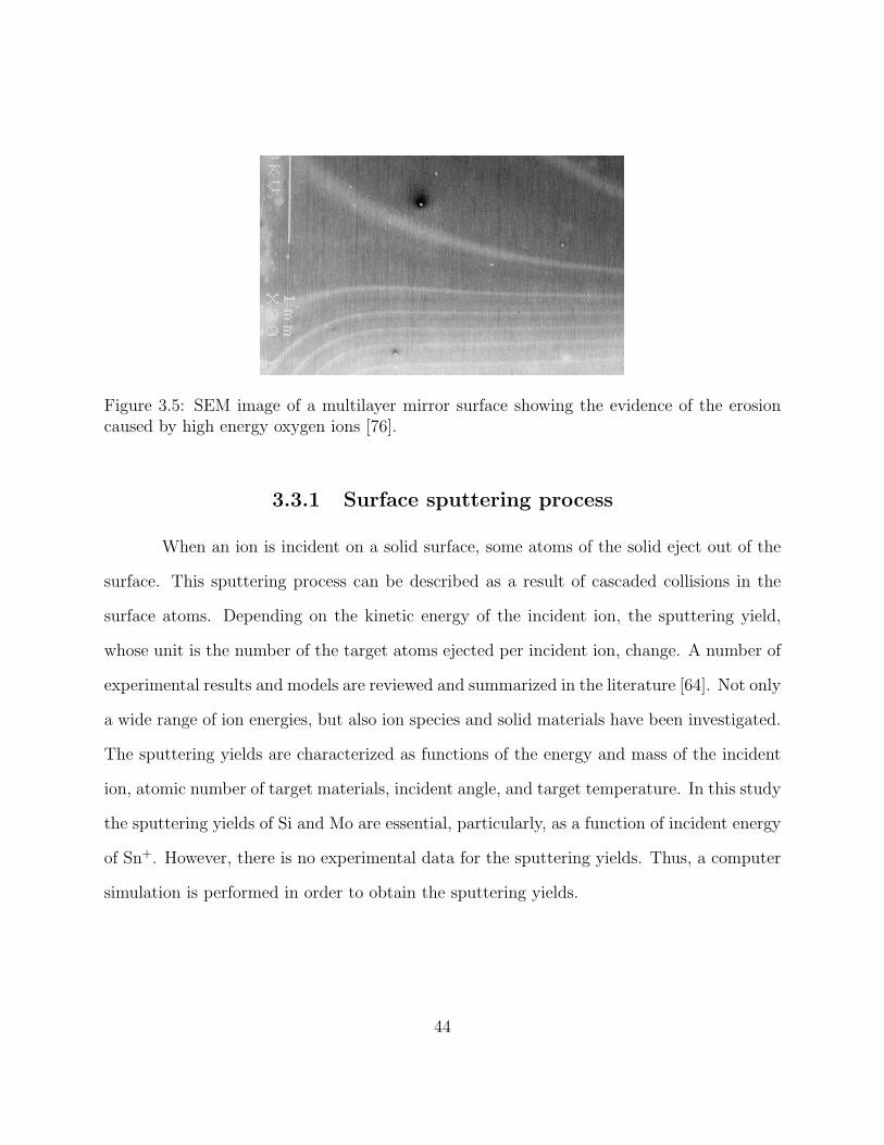
Figure 3.5: SEM image of a multilayer mirror surface showing the evidence of the erosioncaused by high energy oxygen ions [76].
3.3.1 Surface sputtering process
When an ion is incident on a solid surface, some atoms of the solid eject out of the
surface. This sputtering process can be described as a result of cascaded collisions in the
surface atoms. Depending on the kinetic energy of the incident ion, the sputtering yield,
whose unit is the number of the target atoms ejected per incident ion, change. A number of
experimental results and models are reviewed and summarized in the literature [64]. Not only
a wide range of ion energies, but also ion species and solid materials have been investigated.
The sputtering yields are characterized as functions of the energy and mass of the incident
ion, atomic number of target materials, incident angle, and target temperature. In this study
the sputtering yields of Si and Mo are essential, particularly, as a function of incident energy
of Sn+. However, there is no experimental data for the sputtering yields. Thus, a computer
simulation is performed in order to obtain the sputtering yields.
44

3.3.2 A Monte Carlo Simulation - SRIM
Monte Carlo simulations (Monte Carlo method) are widely used for many applica-
tions. The Stopping and Range of Ions in Matters (SRIM), is a Monte Carlo simulation
code that models the collisions in target materials caused by high energy incident ions [77].
One of the results of the simulations is the sputtering yield averaged over specific numbers
of incident ions. It can simulate the sputtering of nearly all the elements for many incident
ion species and all the elements and desired compounds as targets [78]. The calculated re-
sults have been favoritely compared with experimental results [79, 80]. The calculation and
utilization of the results are described in Chapter 6.
3.3.3 Multilayer mirror reflectivity characteristics
As sputtering progresses the total thickness of the periodic structure of the multi-
layer coatings decreases. The consequences of the reduced thickness of the coating, reduced
number of multilayers, results in reduced reflectivity. To illustrate the contribution of the
number of bilayers to the multilayer mirror reflectivity, the reflectivity characteristics are
obtained from the CXRO website [25]. Figure 3.6 shows a lower reflectivity peak but wider
reflectivity band for a smaller number of bi-layers. Based on these characteristics, about
15 bi-layers are allowed to be removed from 40 bi-layer stack to hold high reflectivity to be
within the 10% reflectivity drop limit for mirror lifetime.
45

0
0.1
0.2
0.3
0.4
0.5
0.6
0.7
0.8
12.5 13 13.5 14 14.5
Ref
lect
ivity
Wavelength [nm]
Si/Mo Multilayer mirror reflectivity
N=40N=30N=20N=10
Figure 3.6: Si/Mo multilayer mirror reflectivity characteristics of different number of bilayers[25].
It is possible to extend the mirror lifetime with sacrificial layers on the Si top layer
similar to the capping layers as described before. Theoretically the peak reflectivity can
be improved slightly with increased number of bi-layers [25]. Drawbacks of the sacrificial
layers are the increased manufacturing costs of the mirrors and the possible defects due to
the increased number of layers, such as the surface roughness and the interfacial roughness
between the layers [81].
3.4 Summary of multilayer mirror reflectivity
degradation
It is important to isolate the processes that produce multilayer mirror reflectivity
degradation. Processes like deposition and oxidation do not create any structural degrada-
46

tion. Only a few sub-nanometers of material deposition or only the oxidation of the top layer
is sufficient to attenuate EUV radiation to below the required level. Erosion is a long-term
degradation mechanism and is a result of the mirror surface sputtering caused by high energy
ions generated in the plasmas. Monte Carlo simulations are widely used to predict sputtering
rates. This simulation approach can be used with known ion emission characteristics in terms
of ion flux and kinetic energies to calculate the lifetime of collection optics. To maintain the
required source lifetime requirement, the number of layer pairs in the multilayer mirror can
be reduced from, say 40 to 25, for an ideal case without impairment of the reflectivity.
47

CHAPTER 4
EXPERIMENTAL FACILITIES
4.1 Introduction
For studies of debris generation, detection and mitigation, higher repetition rate
plasma sources are needed to simulate the operation conditions. The laser system used
for this study is a 100 Hz Nd:YAG laser system. Debris and debris mitigation studies are
performed separately from radiation and metrology studies in a dedicated vacuum cham-
ber. The tin-doped droplet target is injected into the target chamber and the laser pulse
generation is synchronized so that every laser pulse is focused onto a single droplet target.
Debris is detected in two ways, deposition diagnostics and ion diagnostics. Debris detection
in combination with several mitigation schemes are also carried out. Two different mitiga-
tion schemes are applied; electrostatic field mitigation, commonly referred to as the Repeller
Field, and a combination of foil trap and magnetic field mitigation, called Magnetic Foil
Trap mitigation.
4.2 Experimental facility
4.2.1 High repetition rate (100Hz) Nd:YAG laser sytem
A commercial laser system (Spectra Physics Quanta-ray GCR-190) is used for this debris
study. It is a Q-switched Nd:YAG laser with a maximum laser pulse energy ∼ 300 mJ, the
48

pulse duration is ∼ 10 ns, and the repetition rate is 100 Hz. The laser beam is focused
onto the target using a lens with focal length of either 50 mm or 100 mm. By considering
the reflectivity of the mirrors and the transmission of the optical components from the laser
output to the target, the maximum energy on the target is about 150 mJ. The minimum
focus diameter is calculated to be 80 µm and the maximum intensity at the target is about
3 x 10¹¹ W/cm2. The laser system is shown in Figure 4.1. The average laser output power
is monitored during experiments by a power meter.
Figure 4.1: Photo of the laser system
4.2.2 The target chamber
The vacuum chamber used for this debris study is cylindrical with an inner diameter
of about 20 cm and is equipped with a turbomolecular pump. The low pressure in the target
chamber is kept typically at around 4 x 10⁻⁴ Torr during the experiments. The optical setup
of the chamber is shown in Figure 4.3. The axis of vacuum chamber is indicated by the
49
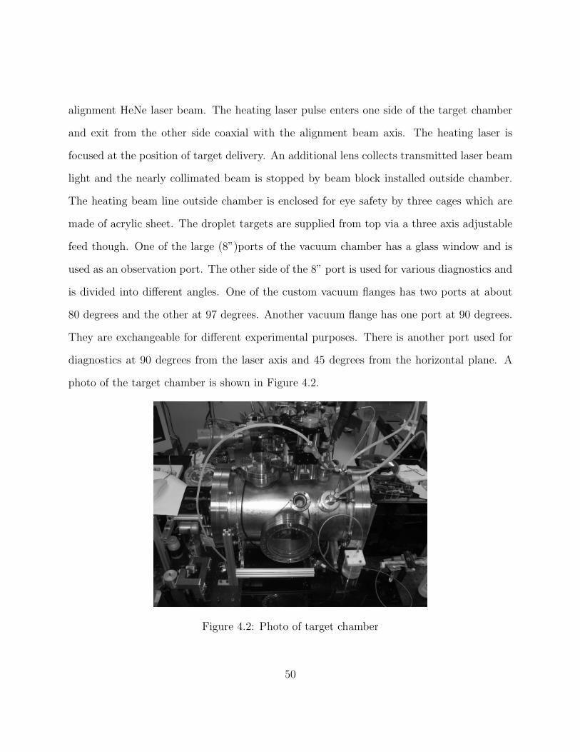
alignment HeNe laser beam. The heating laser pulse enters one side of the target chamber
and exit from the other side coaxial with the alignment beam axis. The heating laser is
focused at the position of target delivery. An additional lens collects transmitted laser beam
light and the nearly collimated beam is stopped by beam block installed outside chamber.
The heating beam line outside chamber is enclosed for eye safety by three cages which are
made of acrylic sheet. The droplet targets are supplied from top via a three axis adjustable
feed though. One of the large (8”)ports of the vacuum chamber has a glass window and is
used as an observation port. The other side of the 8” port is used for various diagnostics and
is divided into different angles. One of the custom vacuum flanges has two ports at about
80 degrees and the other at 97 degrees. Another vacuum flange has one port at 90 degrees.
They are exchangeable for different experimental purposes. There is another port used for
diagnostics at 90 degrees from the laser axis and 45 degrees from the horizontal plane. A
photo of the target chamber is shown in Figure 4.2.
Figure 4.2: Photo of target chamber
50

Nd:YAG lase r
Targe t Ch am be r
O bse rvation port
Strobe lase r diode
Im aging CCD
Lase r dum p
Dia
gno
stic
po
rts
80o
9 0o
9 7o
Focusing le nscolle cting le ns
Im agins obje ctive le ns
Angle s w ith re gards to lase r axis
He
Ne
lase
r
H e Ne alignm e nt be am
Im agins re laying le ns
Figure 4.3: Schematic of optical setting on the target chamber
4.2.3 Target delivery
The target containing 30% tin in a water solution is delivered from a capillary nozzle.
The number of tin atoms doped in a target is near 1013 atoms. The 30 - 100 kHz train of
uniform droplets (from 30 µm to 50 µm in diameter) is generated with a piezo-driven nozzle
assembly and the droplets have a velocity about 20 m/s. The nozzle assembly is mounted
on a 3D translation stage with flexible vacuum bellows so that the position of the droplet is
adjusted from outside chamber. The droplet conditions and stability are monitored by an
imaging system with a CCD camera having an optical resolution of approximately 2 µm. The
illumination of the imaging is made by a laser diode and is delivered from outside chamber as
shown in Figure 4.3. The laser diode is modulated at the same frequency as that is supplied
51

to piezo-crystal but the pulse duration is less than 1µs. With the pulsed laser illumination,
the droplet targets appear as dark circles on the imaging system. The frequency of piezo
signal can be changed in order to have stable target delivery. Unused targets are captured
by a cryogenic cold trap in order to prevent evaporation in the vacuum chamber. Figure 4.4
shows orientations of the target delivery, cold trap, heating laser pulse and imaging system.
4.2.4 Target laser synchronization
The synchronization of the laser pulse and the droplet target is accomplished by
electrical signal synchronization of droplet signals and laser flash lamp trigger signals in
combination with a delay generator and mechanical translation. The laser operates at around
100 Hz while the droplet targets are generated at a frequency of 30 kHz to 100 kHz. The
droplet and laser frequencies are synchronized by a phase lock loop (PLL) circuitry. The
synchronization is performed at a higher frequency ∼ 4 MHz and the signals are divided
by counters to provide stable signals. The signal with the lower frequency passes through
an adjustable delay circuit then goes to the flash lamp trigger on the laser system. It is
reasonable to assume that there is constant delay from the flash lamp trigger signal to actual
laser pulse generation in the laser system. It is also a reasonable assumption that the droplets
travel at constant velocity due to no air drag in the vacuum environment. As described in
Chapter 2, the droplet generation is periodic and that the sizes and velocities are uniform.
Based on these assumptions, only adjustment of the delay is required to synchronize the
laser pulse and target. The timing diagram of the synchronization is shown in Figure 4.5.
A custom synchronization system has been designed and built to have all the functionalities
of PLL, divider, and delay circuit. The synchronization system is operated by a PC by
communicating over the parallel port.
52
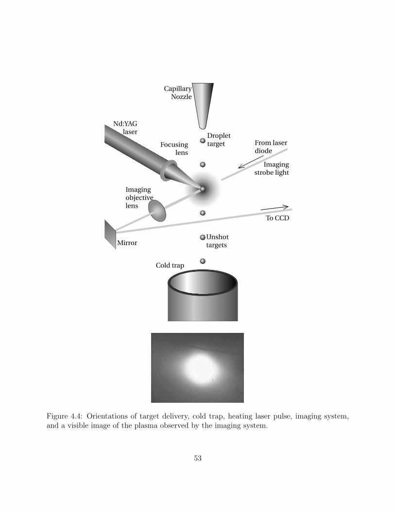
Capillary Noz z le
Nd:YAG lase r
Focusing le ns
Im aging strobe ligh t
Im aging obje ctive le ns
D rople t targe t
Unsh ot targe ts
Cold trap
To CCD
From lase r diode
M irror
Figure 4.4: Orientations of target delivery, cold trap, heating laser pulse, imaging system,and a visible image of the plasma observed by the imaging system.
53

Piezo signal
laser flash lamp trigger
Laser signal
laser gain
laser Q-SW HV
laser pulse
Droplet existance at focus
Figure 4.5: Timing diagram of droplet and laser synchronization
4.3 Debris diagnostics
The primary purpose of this study is to detect debris. The detection can be ac-
complished by observing evidence of debris emission and deposition/erosion and a common
method is to use a witness plate capture. The samples are characterized separately after
the capture, post shot, utilizing different types of characterization facilities. It is an ext-situ
detection. It is also possible to detect debris in-situ utilizing acoustic wave sensors. Any
shifting in surface acoustic oscillation or bulk acoustic oscillation caused by mass transfer can
be detected. Analysis on the frequency shifting requires knowledge of different characteris-
tics of deposited materials. Detecting plasma expansion is also an in-situ characterization.
There are different kinds of charged particle detection in plasmas. A Faraday cup ion probe
and ion spectrometers are used in this study.
54

4.3.1 Witness plate capture and post shot analysis
Glass plates, silicon wafers, and multilayer mirrors are used as witness plates in order
to capture debris particularly deposits. The witness plates are installed in the target chamber
and exposed to the plasma source for a specific time duration where the number of plasma
creations is known. The witness plates are removed from the chamber after the exposure
and then analyzed by using different types of surface characterization methods. The charac-
terization facilities that are used in this study are Optical Microscopy (OM), Atomic Force
Microscopy (AFM), Scanning Electron Microscopy (SEM), Auger Electron Spectroscopy
(AES), X-ray Photon Spectroscopy (XPS), Rutherford Backscattering Spectroscopy (RBS),
and an optical 3D profiler.
A variety of witness plate installations are possible and are applied throughout this
study, an example of which is shown in Figure 4.6. A custom built witness plate holder with
kinetic motion feed-through is mounted on a vacuum flange. The plate can be installed and
uninstalled during an experiment without having to bring the entire chamber to atmosphere.
A photo of the sample holder is shown in Figure 4.6. Typically the witness plate samples
are placed at distances which are equivalent to the distance of the collector mirror, about
10 to 20 cm. If it is assumed that the tin atom emissions from a single target are uniformly
distributed into the entire solid angle, the tin deposition rate is in the order of 10−12 g/cm2
per laser shot. Here the total mass of tin inside a target as described in Chapter 2 is
used. By using the density of solid tin of 7.3 g/cm3, the number of laser shots required
to have tin deposition of 0.75 nm is more than 106 shots. This thickness is the maximum
tin deposition permissible on the collector mirror surface. It is challenging to demonstrate
uniform deposition at the distances using the witness plate capturing method with the 100
Hz laser, which can take at least 3 hours without any sputtering considerations. During the
55

long term exposure of the witness plate, the laser-target interaction condition can change
causing tin aerosol generations and depositions, which are described in Chapter 5. However,
it is a very useful method to observe the aerosol generation and the deposition which are
discussed in Chapter 5.
50 - 150 m m
Laser b eam
Plasm a
Plate h older
Gate
Valve
Liner m otion
fe ed -th ough
Figure 4.6: Experimental setup for (top) witness plate and (bottom) sample holder
56

4.3.2 Deposition monitor
A quartz crystal microbalance (QCM) is a widely used to detect material deposition
on crystal surfaces especially in plasma process facilities such as chemical vapor deposition
(CVD) systems. The acoustic oscillation frequency is a function of deposition mass on the
crystal surface as well as the crystal temperature. It is usually used in combination with
another crystal that is shielded from the deposition, to compensate for any temperature
shift. Typical sensitivities of QCM’s [82] are ∼ 10−9g/cm2Hz depending on the fundamental
frequencies. The frequency of oscillation is in MHz range. It is challenging to detect the
deposition level at the collector mirror equivalent distances. A more sensitive device than
the QCM is a surface acoustic wave (SAW) oscillator [83, 84]. However, this is even more
sensitive to the ambient temperature [85]. These monitors can be better used for high
repetition rate plasma sources, which are discussed in Chapter 8.
4.3.3 Faraday cup ion probes
Ion probes are widely used, not only in EUVL source research, but also in other
plasma related areas of research [75, 86, 87, 88, 89, 90]. The ion probes used in this study are
custom designed to measure the low flux of ions expected from the low mass plasma targets.
A schematic is shown in Figure 4.7. The ion probe collects all the charged particles unless an
electrostatic potential is applied to the grid located in front of the cup electrode. To measure
positively charged ions, a negative potential of approximately -60 V is typically applied. The
ion probes detect the burst of X-ray radiation from the source, generating photoelectrons
on the cup electrode. This photoelectron signal determines the plasma event time used for
time-of-flight (TOF) ion measurements. From the TOF, and the distance between the ion
probe and the source, and the velocity of the ions can be determined assuming they have
57

constant velocity. If the ion species that are producing the signal are known, then the ion
kinetic energies can be calculated from the known mass of the ions.
50 - 150 m m
Laser b eam
Target ch am ber
Plasm a
~-60V
Ion probe
O scilloscope
Figure 4.7: Schematic of Faraday cup ion probe
4.3.4 Ion spectrometer with electrostatic ion energy analyzer
While the IP collects a variety of ions, an electrostatic ion energy analyzer (ESIEA)
ion spectrometer detects selected ions with a corresponding kinetic energy. Figure 4.8 shows
the schematic of the ion spectrometer. The spectrometer consists of an ion flux limiting
aperture, a field-free path for TOF analysis, an energy analyzer, and an ion detector. The
diameter of the aperture is 1 mm which selects a known fraction of the ion flux, and is placed
at the distance of 10 cm from the source, equivalent to the distance of the first collector mirror
in an EUVL source system. Behind the aperture, a separate vacuum chamber is attached to
the target chamber as a field-free drift region for separating each ion species as they move at
58

different velocities. The vacuum of the entire ion spectrometer assembly is kept at less than
1.0 x 10⁻⁶ Torr. The geometry of the ESIEA consists of a set of two electrodes with the
shape of a circular quadrant. Two 1 mm slits are placed at the entrance and the exit of the
analyzer. By changing the applied potentials of the electrodes, one can selectively analyze
the ions with the kinetic energies (KE) having different charge states (Z) and mass (M).
The ion detector placed right after the analyzer detects those filtered ions with the same
KE/Z and different TOF. A single channel electron multiplier (CEM) is used for detecting
the filtered ions. The distance from the plasma to the CEM is 900 mm. Thus a complete ion
spectrum can be obtained by a series of ion measurements with the ESIEA set for different
values of KE/Z.
O scilloscope
Target
Ch am ber
Plasm a
Laser b eam
Turbo
Pum p
100 m m
Apterture
TO F Field fre e path
Analyzer
~-3k V
-2k V
CEM
Figure 4.8: Schematic of (ESIEA) ion spectrometer
59
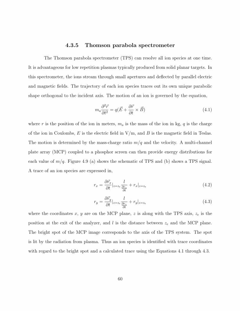
4.3.5 Thomson parabola spectrometer
The Thomson parabola spectrometer (TPS) can resolve all ion species at one time.
It is advantageous for low repetition plasmas typically produced from solid planar targets. In
this spectrometer, the ions stream through small apertures and deflected by parallel electric
and magnetic fields. The trajectory of each ion species traces out its own unique parabolic
shape orthogonal to the incident axis. The motion of an ion is governed by the equation,
ma∂2~r
∂t2= q( ~E +
∂~r
∂t× ~B) (4.1)
where r is the position of the ion in meters, ma is the mass of the ion in kg, q is the charge
of the ion in Coulombs, E is the electric field in V/m, and B is the magnetic field in Teslas.
The motion is determined by the mass-charge ratio m/q and the velocity. A multi-channel
plate array (MCP) coupled to a phosphor screen can then provide energy distributions for
each value of m/q. Figure 4.9 (a) shows the schematic of TPS and (b) shows a TPS signal.
A trace of an ion species are expressed in,
rx =∂~rx
∂t|z=ze
l∂rz
∂t
+ rx|z=ze (4.2)
ry =∂~ry
∂t|z=ze
l∂rz
∂t
+ ry|z=ze (4.3)
where the coordinates x, y are on the MCP plane, z is along with the TPS axis, ze is the
position at the exit of the analyzer, and l is the distance between ze and the MCP plane.
The bright spot of the MCP image corresponds to the axis of the TPS system. The spot
is lit by the radiation from plasma. Thus an ion species is identified with trace coordinates
with regard to the bright spot and a calculated trace using the Equations 4.1 through 4.3.
60

M CP &
Ph osph or
Scre en
Parallel
Electric &
M agnetic Field
Analyzer
Aperture
Plasm a
2
0
0
m
m
8
8
0
m
m
(a) (b)
Figure 4.9: (a) Schematic of TPS, (b) Ion signals measured by TPS
4.3.6 Amplified ion probe
For ion flux measurements with two mitigation schemes, which are discussed in
Chapter 7, ion flux becomes so low that IP cannot detect ions efficiently. The amplified ion
probe is constructed in order to detect low ion flux. Similar to the ESIEA spectrometer, a
single channel electron multiplier (CEM) is used as an ion detector. A negative high voltage
(- 3 kV) is applied to the CEM. The amplified signal is monitored by an oscilloscope. An
aperture whose diameter is 2 mm separates the ion probe section from the target chamber
in order to have high vacuum by a turbo pump. The CEM distance from the plasma source
is 250 mm. The schematic of the amplified ion probe is shown in Figure 4.10.
61

Target Chamber
-3 kV
CEMAperture
Turbo Pump Oscilloscope
Figure 4.10: Schematic of amplified ion probe
4.4 Mitigation schemes
Preventing mirror reflectivity degradation by applying different mitigation schemes is
the second objective of this study and two types of mitigation schemes are applied. Electro-
static field mitigation (Repeller Field) applies a static potential between the plasma source
and witness plates or ion diagnostics. Similarly Magnetic Foil Trap mitigation (MFT) is
placed between the plasma source and the debris diagnostics. Based on the different mitiga-
tion concepts for the two mitigation schemes, the Repeller Field mitigation is installed close
to the diagnostics while the Magnetic Foil Trap mitigation is installed close to the plasma
source.
62

4.4.1 Electrostatic field mitigation
The Repeller Field mitigation concept is to repel charged particles before they reach
the collector mirror surface. All charged particles experience the electric field. The particles
are repelled when the forces generated by the electric field and the charge of the particles
are large enough. Figure 4.11 shows the concept. The evaluation of the effectiveness of the
field is carried out by using witness plates or ion diagnostics.
Figure 4.11: Concept of repeller field mitigation
Figure 4.12 shows an example of how the Repeller Field mitigation is installed with IP
ESIEA, and witness plate diagnostics. A mesh electrode is used to apply the field potential,
which is up to ∼ 600 V without having discharge between the electrode and the chamber.
The distance between the electrode and the grounded collimator is 5 mm and the length
of the collimator is 25 mm. The electric field at the center of the collimator entrance is
calculated to be ∼ 1 x 10⁵ V/m. The IP and witness plates are installed right after the
63
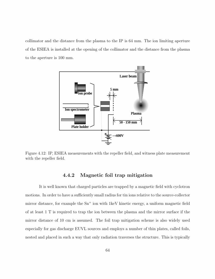
collimator and the distance from the plasma to the IP is 64 mm. The ion limiting aperture
of the ESIEA is installed at the opening of the collimator and the distance from the plasma
to the aperture is 100 mm.
50 - 150 m m
Laser b eam
Plasm a
Plate h older
~<600V
Ion probe
5 m m
Ion spectrom eter
Figure 4.12: IP, ESIEA measurements with the repeller field, and witness plate measurementwith the repeller field.
4.4.2 Magnetic foil trap mitigation
It is well known that charged particles are trapped by a magnetic field with cyclotron
motions. In order to have a sufficiently small radius for tin ions relative to the source-collector
mirror distance, for example the Sn+ ion with 1keV kinetic energy, a uniform magnetic field
of at least 1 T is required to trap the ion between the plasma and the mirror surface if the
mirror distance of 10 cm is assumed. The foil trap mitigation scheme is also widely used
especially for gas discharge EUVL sources and employs a number of thin plates, called foils,
nested and placed in such a way that only radiation traverses the structure. This is typically
64

used with buffer gas or gas flow which makes particles straggle, bounce back and forth with
the collision between the particles and the buffer gas atoms. The straggled particles are
trapped by the foils. Because the configuration of the laser plasma EUVL sources where the
radiation from the plasma is collected by a normal incident mirror and is reflected back to
the IF, see Figure 1.4, it is impractical to enclose the plasma source with a foil trap and gas.
The Magnetic Foil Trap mitigation utilizes both magnetic field and foil traps. The
magnetic field is used to deflect charged particles instead of a gas flow. Thus in this config-
uration the field is transparent to the radiation. In addition it utilizes only two permanent
magnets with surface magnetic field of ∼ 1 T, where the field strength around the plasma
is reduced to ∼ 100 mT due to the low permeability of the vacuum. The details of the
mitigation scheme are discussed in Chapter 7. In order to investigate the effectiveness of the
mitigation scheme, a single channel Magnetic Foil Trap is used, which is shown in Figure
4.13. Ion diagnostics, typically IPs are used to evaluate the effectiveness. Due to the limited
diagnostic ports and physical space, the magnetic field is applied orthogonal to the heating
laser axis. The magnetic field axis and foil trap channel are also orthogonal but 45 degrees
from the horizontal plane. The magnetic field is provided by a set of permanent magnets
and linked together with an iron core, which are shown in Figure 4.14. The foil angle, which
is the angle the two plates make, can be adjusted for different experimental conditions. The
distance from the plasma to the inner side of foils is typically 30 mm, and the outer side
distance is about 100 mm. Figure 4.14 shows its photo.
65
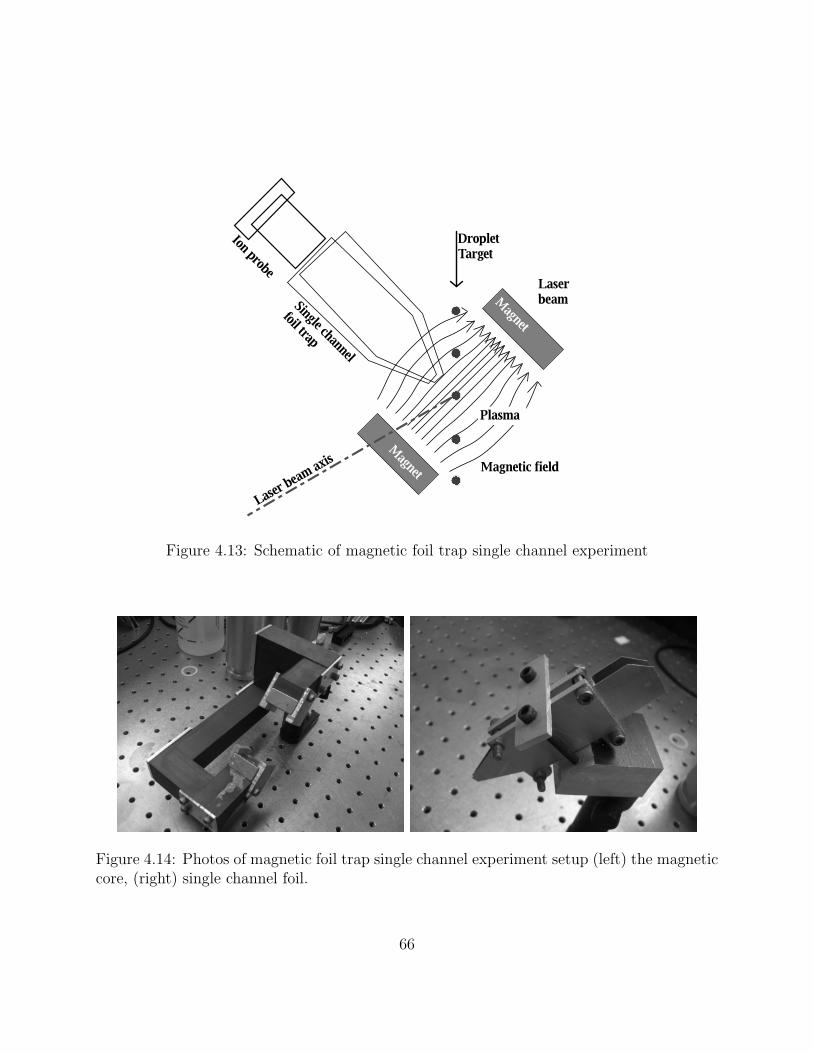
Figure 4.13: Schematic of magnetic foil trap single channel experiment
Figure 4.14: Photos of magnetic foil trap single channel experiment setup (left) the magneticcore, (right) single channel foil.
66

4.5 Summary of experimental facilities
The experimental facilities including the laser system, the target chamber, the target
delivery, and the synchronization are described. The debris detection techniques as well as
the ion characterization techniques are discussed. The two debris mitigation schemes applied
to this study are also described. By utilizing the witness plate post shot analysis, particulate
debris emission characteristics and their impacts on the collector mirrors are discussed in
Chapter 5. The ion emission from the tin-doped droplet plasma is characterized extensively
using the ESIEA ion spectrometer in Chapter 6. The estimation of the mirror lifetime based
on the characterized ion energy distributions as well as the detailed plasma expansions are
also discussed in Chapter 6. The effectiveness of the mitigation schemes are evaluated in
Chapter 7 in terms of reducing particulate debris and ion flux at the collector mirror distance
from the plasma.
67

CHAPTER 5
PARTICULATE DEBRIS - AEROSOLS
5.1 Introduction
In this chapter the formation and characterization of particulate debris from the
tin-doped droplet target are discussed. This target, specifically designed to minimize this
debris, is reduced and the volume is comparable to, or even smaller than, the focus diameter
of the laser pulse. The particulate debris depositions are observed on the witness plates.
These deposits are identified as tin and their thicknesses are characterized. Due to the high
absorption in tin for EUV radiation, as a deposit in the collection mirrors, the aerosols are
lethal to the collector mirrors. The aerosol generation processes are investigated. It is found
that the aerosol generation is minimized by optimizing laser pulse energy coupling to the
target.
5.2 Aerosol deposition on witness plates
The idea of using mass-limited targets is to eliminate debris generation. However, the
initial witness plate sample shows that there is still some particulate matter deposited on the
surface as the plasma is produced from the tin-doped droplet. The deposits appear as thin
splashes, supporting the notion that they are deposited at high velocities. It is reasonable to
expect that these deposits are tin aerosols since there is no other metal element present in
the target. Investigation of how the aerosols are generated, identification of the elements on
68
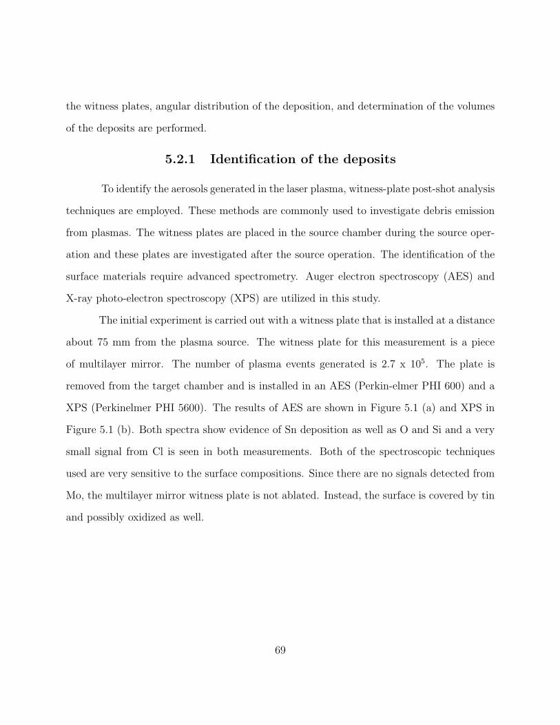
the witness plates, angular distribution of the deposition, and determination of the volumes
of the deposits are performed.
5.2.1 Identification of the deposits
To identify the aerosols generated in the laser plasma, witness-plate post-shot analysis
techniques are employed. These methods are commonly used to investigate debris emission
from plasmas. The witness plates are placed in the source chamber during the source oper-
ation and these plates are investigated after the source operation. The identification of the
surface materials require advanced spectrometry. Auger electron spectroscopy (AES) and
X-ray photo-electron spectroscopy (XPS) are utilized in this study.
The initial experiment is carried out with a witness plate that is installed at a distance
about 75 mm from the plasma source. The witness plate for this measurement is a piece
of multilayer mirror. The number of plasma events generated is 2.7 x 10⁵. The plate is
removed from the target chamber and is installed in an AES (Perkin-elmer PHI 600) and a
XPS (Perkinelmer PHI 5600). The results of AES are shown in Figure 5.1 (a) and XPS in
Figure 5.1 (b). Both spectra show evidence of Sn deposition as well as O and Si and a very
small signal from Cl is seen in both measurements. Both of the spectroscopic techniques
used are very sensitive to the surface compositions. Since there are no signals detected from
Mo, the multilayer mirror witness plate is not ablated. Instead, the surface is covered by tin
and possibly oxidized as well.
69

Figure 5.1: (a) Auger electron spectrum taken from the witness plate and (b) X-ray photo-electron spectrum taken from the same plate sample.
(a)
(b)
However, the sampling area of both these spectroscopic methods is rather large com-
pared to the size of the deposited aerosols. Further analysis on the witness plate surface is
performed by using AES with ”point survey”, which provides better spectral details from
70

a small surface area. ”Point survey” or ”point Auger analysis” is performed by aiming the
incident electron beam to a point of interest and recording the Auger electron spectrum.
Two spectra are taken by the AES point survey. One is from the deposited aerosol
and the other one is from the surface without any deposits for comparison. Figure 5.2 shows
the comparison of AES spectra from the two points. By comparing Sn signals in the two
spectra, the signal of Sn from the deposition is much larger than that from the surface. Thus
the Sn signals in the AES and XPS are from those deposited tin aerosols.
-600
-500
-400
-300
-200
-100
0
100
200
300
400
0 100 200 300 400 500 600 700 800
d[E
N(E
)]/dE
Binding energy [eV]
on depositon surface
Figure 5.2: AES Sn signal comparison on the deposited aerosol.
5.2.2 Profile measurement of the deposits
The same witness plate sample with deposits described above is used to determine
the volume of the aerosols. An AFM (TA instrument µTA-2990) is used to determine the
size of each aerosol. Typical AFM images are shown in Figure 5.3. An area of a 32.5 µm
square was sampled with a resolution of 81 nm. Some of the larger deposits appear in the
71

form of rings. By analyzing the cross section profile of a deposit, the volume of the deposit
can be calculated. The volume of the largest deposit is found to be 7 x 10⁻¹³ cm3 which
likely consists of only tin and its mass is about 5 x 10⁻¹² g. The total mass on tin in the
target is 4.8 x 10⁻⁹ g. There are thousands of these aerosols generated during the laser target
interaction. All the deposits are characterized in term of their volumes since there is a clear
trend of the volume as a function of the diameter of deposits. The trend is shown in Figure
5.4 and the approximation leads to aerosol flux estimation.
Figure 5.3: AFM image of tin deposition on a multilayer mirror.
5.2.3 Aerosol flux calculation
Based on the diameter-volume relationship described above and the density of tin,
the aerosol emission is characterized in terms of the total mass of tin. The mass of tin
deposited in the AES sample area is estimated by categorizing the diameters of deposits
and by counting the number of deposits. Figure 5.5 shows (a) the scanned AES image and
(b) back-scattered AES image. The sample area is 140 µm x 140 µm. The image shown
72

(a) is similar to the SEM image and (b) indicates spatial distribution of high Z materials
on the surface. The spatial distribution of the deposits shown in (a) and (b) are identical.
Since there is no Mo signal detected in AES or XPS, all of the deposits in (a) are counted
in the total mass estimation. The isotropy of aerosol emission is confirmed separately by
the measurement of the angular distribution of deposits [91]. The solid angle of the AES
sample area is calculated with the distance of the plate from the source plasma. The aerosol
emission is estimated to be approximately 40% of total tin mass in the target. During the
laser-target interaction, about one half of the tin contained in the target forms thousands
of small aerosols. After the plasma generation the aerosols are deposited on the collection
optics. Therefore the generation has to be minimized and aerosols have to be mitigated.
0
1e-13
2e-13
3e-13
4e-13
5e-13
6e-13
7e-13
8e-13
9e-13
1e-12
0 1 2 3 4 5 6 7 8 9
Vol
ume
[cm
3 ]
Deposition diameter [µm]
AFMV=1.3x10⁻³Dπ(D/2)2
Figure 5.4: Deposit volume dependency of the diameters.
73

Figure 5.5: (a) AES image 140µm X 140µm, (b) Back-scattered image (Same area).
(a) (b)
5.3 Aerosol generation processes
The number of aerosols generated from the tin-doped droplet laser plasmas is as seen
in the previous section. However, the generation processes of aerosols in tin-doped droplet
plasmas were not fully understood. The target droplet is in a solution form and the size of
the target is smaller than the laser focus. Thus, all the material is being heated by the laser.
The following three analyses suggest that aerosols are generated when the entire target is
incompletely heated by the laser pulse. The laser intensities used in these three studies are
set lower than the optimum.
5.3.1 Aerosol generation in low intensity laser irradiation
Two different doped targets are used in the low intensity laser irradiation experiment.
Tin and copper are doped in water as chloride solutions, and the droplet targets produced
74

with these (a) (b) solutions are irradiated using a low energy pulse. The energy of the laser
pulse is less than 100 µJ which is not enough to produce plasma. The transmitted laser
pulse is detected by a photodiode so that the target and the laser pulse are synchronized.
Glass witness plates are placed at a close distance from the laser focus, 15 mm, in order to
capture low velocity aerosols which are expected to be generated with a low intensity laser
focus. Both witness plates are exposed to over 6 x 10⁴ laser shots. Optical microscopy shows
aerosols deposited on the witness plate surface in both doped target cases.
These experiments indicate that the aerosols are generated with low laser energy,
hence, low laser intensity. However, the temperature of these aerosols is hot enough to
form liquid copper. The melting temperature of copper is 1085 degrees Celsius. There are
many possibilities for the low laser intensity conditions even if the laser pulse energy is the
optimum. If the droplet target is placed off the laser focus, the target experiences low energy
laser irradiation. In fact, the first experiment is performed with a low level synchronization
scheme. In addition, the target droplet generation has velocity fluctuations so that the
operator had to control the target position all the time. Not only the target to be shot
but also adjacent droplets can experience low energy irradiation. The laser light scattered
off the source plasma can irradiate the two adjacent droplets. The radiation of the source
plasma can irradiate the adjacent droplets, as well. In all cases, a low energy laser pulse will
generate aerosols.
5.3.2 Origin of aerosol generation
Aerosol generation can be the result of incomplete heating of the target including
secondary heating of the adjacent targets by the plasma radiation or scattered laser light. In
order to determine the origin of the particle generation, the following procedure is applied.
75

First, a mask with a certain aperture profile is installed between the target and the witness
plate. Second, the target separation is enlarged to eliminate the possibility of having the
adjacent target heated directly or secondarily by the laser. Third, the target formation and
positioning are carefully controlled during the exposure. No unwanted targets are close to
the laser focal region. Lastly, the laser energy is reduced intentionally so that incomplete
heating occurs. The plasma is generated by a 30 mJ laser pulse.
The mask and witness plate configuration are shown in Figure 5.6 (a) and the witness
plate surface image is shown in Figure 5.6 (b). The distance between the transition from the
deposited area to no deposition area is 75.7 µm vertically and 32.4 µm horizontally. With the
geometry shown in Figure 5.6 (a), the size of the origin of the particles is 46.9 µm vertically
and 20 µm horizontally which is equivalent to the size of the target. Thus, the particles are
generated at the target and not at the adjacent targets.
Figure 5.6: (a) distances of target, mask, and witness plate, (b) dark field image of thewitness plate surface.
(a) (b)
76

5.3.3 Laser energy, intensity, focus diameter
Two more witness plate samples are produced using different plasma conditions. One
plasma condition is created using a 30 mJ laser pulse, which is the same condition used for
the particle origin determination experiment. The other condition is created by using a 120
mJ laser pulse which produces the condition for the optimum CE. The exposure is 1.2 x 10⁵
shots for both cases. The witness plates are placed at 81 mm from the plasma, which is
the same as described in Figure 5.6. The SEM images of those two samples are shown in
Figure 5.7. As shown in Figure 5.7 (a), a number of aerosols are deposited on the surface,
whereas only a few deposits are observed in Figure 5.7 (b). This comparison shows the target
material irradiated by low energy laser pulse generates much more aerosols than the target
irradiated by high energy laser pulse.
Figure 5.7: (a) SEM image of witness plate surface exposed by plasma created by 30 mJlaser pulse, (b) by 120 mJ pulse.
(a) (b)
77

There is a relationship between irradiation conditions of high CE and minimum num-
ber of aerosol generation. When the target is irradiated by sufficient laser energy, the entire
target is heated well enough to become plasma which emits EUV radiation. The laser in-
tensity is (a) (b) calculated to be 1.2 x 10¹¹W/cm2 with the laser energy of 120 mJ and
the focus diameter of 100 µm. This intensity is equivalent to the intensity for the optimum
CE [14]. The target diameter is calculated to be 42 µm with the droplet frequency at 30
kHz where the laser focus is more than the twice the target diameter. It is known that the
droplet target starts expanding before the laser pulse reaches its peak [58]. With a typical
plasma expansion velocity of 105 m/s, the plasma expands from 40 µm diameter to 100 µm
diameter in 0.3 ns. Even if a lower velocity is assumed for lower pulse energy before the
peak, the time required for the expansion is approximately 1 ns. Therefore, a larger focus
diameter than the target diameter is required to heat the entire target sufficiently.
5.3.4 Total tin atom emission
At the conditions isolated for obtaining high CE, only a very small number of aerosols
are generated. It is reasonable to expect that the entire target is completely ionized. The
plasma expands only as ions, electrons, and neutral atoms, if recombination of singly ionized
ion takes place. Rutherford Backscattering Spectroscopy (RBS) is performed on the witness
plate sample that was exposed to the plasma at high CE conditions as described previously.
The tin atom concentration on the plate surface obtained from RBS analysis [92] is 2 x
1015 atoms/cm2. The total number of tin atoms is calculated to be 1.6 x 10¹⁸ atoms over
1.2 x 10⁵ laser pulses by assuming isotropic expansion of plasma. The total number of tin
atoms is equivalent to about 18 % of the total mass of tin supplied into the droplet targets.
The number is reasonable since some deviation from isotropic expansion is possible, and tin
78

self sputtering where the tin deposition layer is sputtered by tin ions, is also possible. The
ultimate concept of the mass-limited target is finally realized by optimizing the irradiation
conditions.
5.4 Summary of particulate debris
These experiments on aerosol generation in metal-doped droplet laser plasmas char-
acterize this phenomena when the tin-doped droplet target is heated by laser pulses of dif-
ferent intensities. When the target is not sufficiently heated by the laser pulse, tin aerosols
are generated. The sizes of aerosols range up to a few hundred of nanometers in diameter.
Although the sizes of aerosols are small, the thickness of deposition is enough to attenuate
EUV radiation below the required level. The aerosol generation can be minimized by op-
timizing the laser intensity and focus diameter. When it is optimized, the target is fully
ionized. This fully ionized plasma source is then the source of energetic ions which can cause
mirror erosion. The ion emission characteristics are discussed in the next chapter in great
detail. It is also important to keep the target delivery stability in order to have optimized
laser coupling to the target for long term operation, which is discussed in Chapter 8.
79

CHAPTER 6
ION EMISSION
6.1 Introduction
Once the whole target is ionized, the only threat to the collection optics reflectivity
degradation is ions. High energy ions cause collector mirror surface sputtering. This chap-
ter describes ion emission characteristics, especially, ion kinetic energy distributions at the
collector mirror surfaces. By using the distributions and surface sputtering simulations, ero-
sion rates are estimated. The erosion rates determine the lifetime of the multilayer mirror
reflectivity. The most contributing factor on surface sputtering is high energy ions. The
kinetics of plasma expansion is described by fluid-dynamics plasma simulations. Recombi-
nation processes that determine the ionization stages of ions at the collector mirror distance
are discussed.
6.2 Ion emission characteristics
Ion emission produced by the plasma source can be measured by detecting charges
carried by the expanding plasma. A Faraday Cup Ion Probe (IP) is commonly used to
measure the ion flux. The ion flux measurement with an IP is simple but does not provide
much information on individual ion species or the ionization stages. For example, tin-doped
plasmas contain different mass of ion species ranging from hydrogen, 1 A.M.U. to tin 118.7
A.M.U. The ionization stages can be up to 11 for tin ions at the plasma temperature of 30 eV.
To measure more detailed ion emission, ion spectrometry is necessary. An ion Spectrometer
80
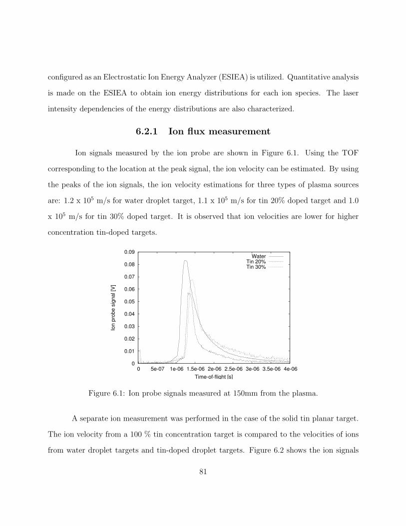
configured as an Electrostatic Ion Energy Analyzer (ESIEA) is utilized. Quantitative analysis
is made on the ESIEA to obtain ion energy distributions for each ion species. The laser
intensity dependencies of the energy distributions are also characterized.
6.2.1 Ion flux measurement
Ion signals measured by the ion probe are shown in Figure 6.1. Using the TOF
corresponding to the location at the peak signal, the ion velocity can be estimated. By using
the peaks of the ion signals, the ion velocity estimations for three types of plasma sources
are: 1.2 x 10⁵ m/s for water droplet target, 1.1 x 10⁵ m/s for tin 20% doped target and 1.0
x 105 m/s for tin 30% doped target. It is observed that ion velocities are lower for higher
concentration tin-doped targets.
0
0.01
0.02
0.03
0.04
0.05
0.06
0.07
0.08
0.09
0 5e-07 1e-06 1.5e-06 2e-06 2.5e-06 3e-06 3.5e-06 4e-06
Ion
prob
e si
gnal
[V]
Time-of-flight [s]
WaterTin 20%Tin 30%
Figure 6.1: Ion probe signals measured at 150mm from the plasma.
A separate ion measurement was performed in the case of the solid tin planar target.
The ion velocity from a 100 % tin concentration target is compared to the velocities of ions
from water droplet targets and tin-doped droplet targets. Figure 6.2 shows the ion signals
81

from the solid tin planar target. The velocity of the peak is calculated to be 5.8 x 10⁴ m/s
which is less than half of the velocity from water droplet targets. This series of ion signals
indicate that doping of tin causes ion signals to slow down. The slower expansion is easily
expected because the mass of a tin atom is significantly larger than the mass of hydrogen
and oxygen ions for the same kinetic energy.
0
0.01
0.02
0.03
0.04
0.05
0.06
0.07
0 2e-06 4e-06 6e-06 8e-06 1e-05 1.2e-05 1.4e-05
Ion
prob
e si
gnal
[V]
Time-of-flight [s]
Solid Tin
Figure 6.2: Ion probe signal from solid tin planer target.
6.2.2 Mass spectrometer
Typical ion spectra are shown in Figure 6.3. The signal from the water target is shown
for (a) KE=250 eV, and the signal from tin 30% doped target is shown for (b) KE=313 eV.
In both signals, the ion probe signals are also shown as references when converted to the
same distance of the CEM in the ion spectrometer.
Signals from different ion species are observed from both types of target. One peak
in ESIEA signal is observed before the peak of the IP signal and is evident for both targets.
Also, at least four lines around the peak and the decaying region in the IP signal are observed.
82

The first ESIEA signal is most likely from hydrogen and the latter signals are from oxygen
(in Figure 6.3 (a)). As expected, four more signals are detected after the later part of the
decay of the IP signal from a tin doped target. More detailed identification, analysis, and
energy distributions are described in the following sections.
-0.08
-0.06
-0.04
-0.02
0
0.02
0 5e-06 1e-05 1.5e-05 2e-05
ES
IEA
sig
nal [
V]
Ion
prob
e si
gnal
[V]
Time-of-flight [s]
ESIEAIon probe
-0.04
-0.03
-0.02
-0.01
0
0.01
0 5e-06 1e-05 1.5e-05 2e-05 2.5e-05 3e-05 3.5e-05 4e-05
ES
IEA
sig
nal [
V]
Ion
prob
e si
gnal
[V]
Time-of-flight [s]
ESIEAIon probe
Figure 6.3: (a) Ion spectrum and ion probe signal from water droplet target, (b) Ion spectrumand ion probe signal from Tin 30% doped droplet target.
(a)
(b)
83

6.2.3 Quantitative ion spectrometer analysis
It is possible to obtain the entire ion spectrum for each ion species by applying a
quantitative analysis on the ESIEA measurements. Each ESIEA signal is based on the num-
ber of ions in a small energy window which are based on the mass-charge ratio. By scanning
the energy window throughout the ion energy range, the ion kinetic energy distributions for
all the ion species are obtained. A series of measurements are necessary and the plasma
conditions for all the measurements must remain same. The following section describes the
quantitative analysis on ESIEA measurements applied to this study.
A typical ESIEA spectrometer signal is shown in Figure 6.4 (a). Several peaks are
observed in the signal because the different components of the target material arrive at the
detector at different times depending on their mass-charge ratio (M/Z). These signal peaks
are generated by ions passing through the analyzer, and hold the relationship expressed by
the following equation.
ZeE =Miv
2i
RA
(6.1)
where Z is ionization state of the ion species, e is the unit charge, E is the transverse electric
field inside the analyzer in V/m, mi is ion mass in kg, vi is ion velocity in m/s, and RA is
the radius of the analyzer path in meters. The ion velocity is determined by the distance of
CEM from the source and the TOF. Then Equation 6.1 can be reorganized in terms of M/Z.
Mi
Z=
eRAE
mpl2(TOF )2 (6.2)
where Mi is the atomic weight of the ion of interest, mp is the proton mass in kg, l is the
ion CEM distance from the plasma in meters, and TOF is the time-of-flight in the signal
in seconds. To identify all the signal peaks, the signal is converted to M/Z based signal
by using Equation 6.2. A typical M/Z signal is shown in Figure 6.4 (b). The M/Z axis is
84
plotted in logarithmic scale. All the peaks in the signal are identified as specific ion species.
By keeping the same plasma conditions, it is possible to obtain M/Z signals with
different energies by changing the electric field strength in the analyzer. It is then possible
to plot all signals together and investigate the signal profile for a constant M/Z, shown in
Figure 6.5 (a). However, because different M/Z spectra are converted from different TOF
signals, the M/Z values in all the signals plotted do not lineup. A simple linear interpolation
must be applied to all the converted signals. This complete map of M/Z spectra at a constant
plasma condition is shown in Figure 6.5 (b). It is possible to make a profile for a constant
M/Z, in other words, slicing the spectral map for each ion species can provide the ion energy
distribution.
To obtain the ion energy distributions for individual ion species, it is necessary to
count the total charge from the CEM signal peak and to calculate the number of ions
analyzed in the energy window of the analyzer. By obtaining the efficiencies of the ion
limiting aperture and the slit of the analyzer entrance, the distribution is calculated in terms
of the number of ions per unit energy. Then the distribution is estimated in terms of the
unit solid angle where isotropic ion emission is assumed. The details of the procedure are
described in the following section and the schematics are shown in Figure 6.6.
85

Figure 6.4: (a) Typical ESIEA signal, (b) converted M/Z signal.
(a)
(b)
86

Figure 6.5: (a) Collected M/Z signals, (b) interpolated M/Z spectral map.
(a)
(b)
87

Figure 6.6: Detailed schematics of ESIEA for quantitative analysis.
To count the number of electrons in each CEM signal peak, it is necessary to specify
the analyzer energy window and the corresponding TOF window. First the nominal ion
kinetic energy of the analyzer is expressed as
KE =1
2RAZeE (6.3)
obtained from Equation 6.1 by expressing 12miv
2i = KE where KE is expressed in J. Because
of the finite width of the slits of the analyzer, the analyzer has an energy window expressed
by the equations.
∆KE = KEmax −KEmin (6.4)
KEmax =1
2
(RA +
1
2∆RA
)ZeE (6.5)
KEmin =1
2
(RA −
1
2∆RA
)ZeE (6.6)
88
where ∆RA is the width of the slit in meters. The corresponding TOF window is expressed
in the following.
∆TOF = TOFmin − TOFmax (6.7)
TOFmax =1
l
√Mimp
2 ·KEmax
(6.8)
TOFmin =1
l
√Mimp
2 ·KEmin
(6.9)
The signal integration can be calculated by multiplying the signal peak value and ∆TOF
because the time constant of the CEM [93] is approximately 4 ns, much smaller than the
acquisition time step of the signal. The number of electrons contributing to the signal peak
can now be calculated using
− 1
e
Vp
Rt
∆TOF (6.10)
where Vp is the signal peak in volt, and Rt is the terminal resistance of the oscilloscope in
Ω. Because the detected electrons are multiplied by CEM based on the incident ions, the
number of the incident ions, ∆Ni, is expressed in
∆Ni = −1
η
1
G
1
e
Vp
Rt
∆TOF (6.11)
where η is the efficiency of CEM, and G is the gain of CEM. Here ∆Ni represents the number
of ions analyzed in the energy window ∆KE. The ratio ∆Ni/∆KE is approximated to the
notation of the energy distribution dN/dE when ∆Ni is approximately constant or ∆KE
is small. Finally, the ion energy distribution in terms of the number of ions per unit solid
angle is obtained by calculating the efficiencies of the slit at the analyzer entrance and the
aperture at known distances.
The following are the values in this study, RA is 25 mm, ∆RA is 1mm which determines
∆KE to be 4.0% of nominal KE. Rt is 50 Ω and G is 106 which is a typical value [93]. η
89

is 0.8 which is reasonable assumption for tin in the range of over 1 keV [80]. The collection
ratio of the analyzer entrance slit is 9.8 x 10⁻² without considering ion beam divergence in
the field free path. The efficiency of the ion flux limiting aperture is 6.3 x 10⁻⁶.
With the calculation described, the ion energy distributions for individual ion species
are obtained. The distributions of different tin ion species at laser intensity of 9.7 x 10¹⁰
W/cm2 are shown in Figure 6.7. Most of the ion emission detected is from low ionization
states, typically less than Sn5+. These lower ionization states that are observed at this
distance from the plasma is compared to the ionization states contributing to the EUV
radiation observed in the dense plasma source (Sn9+ - Sn11+). All the ion distributions
are shown in appendix. The ion distributions are used in estimating the mirror reflectivity
lifetime in a later section.
1.0e+03
1.0e+04
1.0e+05
1.0e+06
1.0e+07
1.0e+08
1000 10000
dNsr
-sho
t / d
E
Ion kinetic energy [eV]
Sn+
Sn2+
Sn3+
Sn4+
Sn5+
Figure 6.7: Tin ions energy distributions at intensity of 9.7 x 10¹⁰ W/cm2.
90

6.2.4 Emission dependency on the laser intensities
Ion emission characteristics are measured at different laser intensities. The ion probe
measurements indicate that the increased plasma expansion velocities occur at higher laser
intensities. Figure 6.8 shows the comparison between ion signals at different laser intensities.
The plasma expansion velocities are measured to be 8.9 x 10⁴, 1.0 x 10⁵, and 1.4 x 10⁵ m/s at
intensities of 9.7 x 10¹⁰, 1.9 x 10¹¹, and 2.8 x 10¹¹ W/cm2 respectively. The plasma expansion
velocity increases about 50 % when the laser intensity is increased by three times.
0
0.01
0.02
0.03
0.04
0.05
0.06
0 5e-07 1e-06 1.5e-06 2e-06 2.5e-06
IP s
igna
l [V
]
Time-of-flight [s]
9.7e10 W/cm2
1.9e11 W/cm2
2.8e11 W/cm2
Figure 6.8: Ion probe signals at different laser intensities at 125 mm distance from theplasma.
Ion energy distributions at different laser intensities are characterized. Higher kinetic
energies and higher populations in higher ionization states are observed in higher laser in-
tensities. The kinetic energy shift to higher energy can be explained by the higher plasma
temperature due to the higher laser intensities. Higher ionization states can be the result
of lower recombination rates at the high temperature, as seen in Equation 2.16. Ion ki-
netic energy distributions of oxygen ions and tin ions at three different laser intensities are
91

shown in Figure 6.9 and Figure 6.10 to illustrate these trends in different ion species. For all
species including the distributions which are not shown, general trends mentioned above are
observed. Another trend that is observed is a large slope in the high energy region of each
ion energy distribution, especially for the singly and doubly ionized species. The population
differences are large in the low energy side of the slope and high energy side of the slope.
The difference ranges from one order of magnitude to three orders of magnitude within the
ion populations. However, as illustrated in the case of ion energy distribution of Sn5+, peaks
in population are observed at the high energy side. These peaks are seen to shift to higher
energy when the laser intensity is increased. The peaks correspond to the kinetic energy
with the plasma expansion velocities measured by ion probes and also they are calculated in
fluid simulations which are discussed later in this chapter.
92

1.0e+03
1.0e+04
1.0e+05
1.0e+06
1.0e+07
1.0e+08
1000 10000
dNsr
-sho
t / d
E
Ion kinetic energy [eV]
I=9.7e10 W/cm2
I=1.9e11 W/cm2
I=2.8e11 W/cm2
1.0e+03
1.0e+04
1.0e+05
1.0e+06
1.0e+07
1.0e+08
1000 10000
dNsr
-sho
t / d
E
Ion kinetic energy [eV]
I=9.7e10 W/cm2
I=1.9e11 W/cm2
I=2.8e11 W/cm2
1.0e+03
1.0e+04
1.0e+05
1.0e+06
1.0e+07
1.0e+08
1000 10000
dNsr
-sho
t / d
E
Ion kinetic energy [eV]
I=9.7e10 W/cm2
I=1.9e11 W/cm2
I=2.8e11 W/cm2
Figure 6.9: Ion kinetic energy distributions of (a) O+, (b) O2+, (c), and O5+.
(a)
(b)
(c)
93

1.0e+03
1.0e+04
1.0e+05
1.0e+06
1.0e+07
1.0e+08
1000 10000
dNsr
-sho
t / d
E
Ion kinetic energy [eV]
I=9.7e10 W/cm2
I=1.9e11 W/cm2
I=2.8e11 W/cm2
1.0e+03
1.0e+04
1.0e+05
1.0e+06
1.0e+07
1.0e+08
1000 10000
dNsr
-sho
t / d
E
Ion kinetic energy [eV]
I=9.7e10 W/cm2
I=1.9e11 W/cm2
I=2.8e11 W/cm2
1.0e+03
1.0e+04
1.0e+05
1.0e+06
1.0e+07
1.0e+08
1000 10000
dNsr
-sho
t / d
E
Ion kinetic energy [eV]
I=9.7e10 W/cm2
I=1.9e11 W/cm2
I=2.8e11 W/cm2
Figure 6.10: Ion kinetic energy distributions of (a) Sn+, (b) Sn2+, (c), and Sn5+.
(a)
(b)
(c)
94
6.3 Erosion study
Understanding the details of the ion flux and kinetic energies, as well as the resulting
damage on the collector mirror surfaces is important in obtaining a complete picture of the
effect of ion emission on the collector mirror. However, erosion is a very slow degradation
process. The evaluation of surface sputtering requires long term exposures. It is therefore
challenging to detect erosion at the mirror distance especially for low ion emission from
tin-doped target plasmas. The current experimental setup for long term exposure is also
limited by the laser repetition rate (100 Hz) of the laser used. Therefore, Monte Carlo
simulations are adopted to study erosion on the multilayer mirrors. The sputtering rates
of Mo and Si are calculated with measured ion kinetic energy distributions. From this
analysis the estimated mirror lifetime is about two orders of magnitude lower than the
lithography roadmap requirement. Although this appears a formidable difference, this level of
mirror degradation is many orders of magnitude less than all other plasma sources currently
under development. To satisfy the roadmap requirement, mitigation is necessary and this is
discussed in the next chapter.
6.3.1 Limitation of laser repetition rate
The precise estimation of mirror lifetime is carried out using the measured ion en-
ergy distributions at the mirror distance and the surface sputtering simulations, instead of
compromising expensive collector mirror over the large number of plasma generation cycles.
The main reason for this estimation approach is because the plasma generation cycles in the
facility used in this study is limited by the later repetition rate, which is only 100 Hz and the
required number of plasma events is in the order of 1011. Generating this many events using
a 100 Hz laser will take about 300 years! Even if a high repetition laser is used to generate
95
the plasma at the specified repetition rate in the EUVL source requirements, it will take a
few years to reach the required number of plasma generation cycles. Therefore, estimating
the mirror lifetime using the kinetic energy distributions and the surface sputtering yields
is a reasonable method for any EUVL light sources development. This is the first time this
approach has been adopted to estimating the lifetime of the collection mirrors. As described
in Chapter 3, no experimental reference is available for Si and Mo surface sputtering on tin
ion bombardments in different kinetic energies. Thus the widely used SRIM simulation code
[78] is used to calculate the sputtering yields of Si and Mo on the tin ion bombardment.
6.3.2 Lifetime estimation of mirror reflectivity degradation
Figure 6.11 shows the SRIM calculations of the incident ion energy dependences of
sputtering yields for Si and Mo surfaces. The sputtering yields in the range of 400 eV to
10 keV are approximated using the least square methods. The integration of the sputtered
Si and Mo atoms from the mirror surface over the ion kinetic energy range determines the
sputtering rate. The number of laser shots needed to remove 1 nm thickness of Si is calculated
to be 1.52 x 10⁸ and for Mo, it is 1.45 x 10⁸. For a typical multilayer mirror structure, the
thickness of a Si/Mo layer pair is 6.9 nm, the ratio of Mo in the layer pair is 0.4, and the
peak reflectivity at 13.5 nm is approximately 73% [25]. The peak reflectivity drops from 73%
to 66% when the number of the layer pairs is reduced from 40 to 25. It is assumed therefore
the required number of laser shots before the mirror reflectivity falls below 66%, will be 1.55
x 1010. Here, it is assumed that the distance of the mirror surface from the plasma is 20 cm
and the sputtering yields are the same for Sn+ to Sn5+ ions.
Based on the sputtering rate, the calculated operation time is approximately 600
hours with a 7 kHz source repetition rate, as stated in the source requirements. However the
96

estimated EUV power at IF is lower than the required power when the current tin-doped
droplet target is operated at that repetition rate. The laser energy per pulse used is about
100 mJ. With a CE of 2%, the emitted EUV energy into 2π is 2 mJ. When the source is
operated at 7 kHz, the EUV power at the IF will only be 7W assuming 2π collection and 50
% mirror reflectivity.
To satisfy the power requirement, the laser energy can be increased by, at least, a
factor of at least 10 or the repetition rate can be increased by a factor of 10. Assuming
that CE of 3% can be achieved, then the EUV power at IF will be 105 W. This is close
to the source power requirement of 115 W. Increasing CE may be possible by optimizing
the irradiation configuration [14]. Increasing the laser energy is challenging, not only for
the laser systems but also for maintaining the optimum CE with the increased laser energy.
The laser intensity with the increased laser energy will be greater than the optimum for the
current target geometry.
1
10
1000 10000
Spu
tterin
g yi
eld
Incident tin ion energy [eV]
SiMo
0.0058x0.665
0.0106x0.645
Figure 6.11: The incident ion energy dependencies of the sputtering yields for Si, Mo surfaces.(SRIM calculations)
97

Increasing the repetition rate can be challenging from the laser viewpoint. It can be
considered as a single laser system or multiple laser systems can be temporally multiplexed
to achieve higher rates. The target repetition rate of up to 100 kHz is already demonstrated.
However, the penalty for increasing laser repetition rate with the same size of target is
increased ion emission. The lifetime of the collection optics will be shortened by a factor of
10 at 70 kHz laser repetition rate. Therefore the estimated lifetime of the collector mirror is
60 hours at 70 kHz which is a factor of 500 shorter than the requirement. Thus, ion mitigation
with a reduction ratio of at least 500 is necessary to satisfy the lifetime requirement.
6.4 Plasma expansion simulation
As described in Chapter 2, it is possible to calculate and estimate the details of
plasma expansion at different laser intensities. The expressions for particle motion and en-
ergy transport are presented. The initial target condition is also known in terms of density,
size, and concentration of materials. Different levels of approximation can be applied. An
isotropic energy deposition and evolution of plasmas can be assumed. It is also possible to
include a 3D description of plasma and spatial distribution of laser intensities. The fluid
species in the plasma can be individual ion species or an averaged species. For droplet laser
plasmas, simulations in one dimensional spherical coordinate agree well with experimental
measurements. The electron density profiles are measured using interferometry, and both
measurements and simulations agree [58]. The spectrum measured at different laser intensi-
ties correspond to the ion populations at the electron temperatures as was predicted [14]. In
the following sections, a discussion on the plasma expansion calculated using the simulations
are compared with measured ion flux characteristics.
98
6.4.1 Simplified model of fluid simulations
Tin doped droplet target based plasma generation and expansion are described using
a simplified model. The ultimate goal of this model is to describe the details of plasma
expansion of a multi-component target. Tin-doped droplet target is an appropriate target,
with spherical geometry that can be described in 1D.
The model divides the target into a number of small sections called cells. Each cell has
geometrical properties, fluid properties, and plasma properties. The geometrical properties
are position, width, area; thus volume. The fluid properties are mass, pressure, density,
velocity, and temperature. The plasma properties are a product of species, ionization state,
and interactions between species, which supplements the fluid properties. A fluid contains
two different species, which are electrons and different ions. An electric field is described as
part of the fluid. It is assumed that no magnetic field is applied and the current induced
magnetic field is negligible. The concept is illustrated in Figure 6.12.
A C++ code is written to execute the model, and the code declarations and processes
are shown in the appendix. Each cell has the properties of position, size, velocity pressure,
mass, density, temperature, ionization state, external force, time derivatives of density, ve-
locity, and temperature. The scalar properties of position and size as well as the vector
property of velocity can be expressed in 3D. The external force is a vector sum of force due
to Lorentz forces and friction forces caused by coulomb collisions with other species. The
time derivatives are calculated as described in Equations 2.9 through 2.11. In the energy
balance equation, the power transferred to the cell is the sum of absorbed laser energy and
energy transfer to ions, which is usually negative. The energy loss due to radiation is not
included in this model but it can be implemented with appropriate assumptions, such as
blackbody radiation. The ionization state is calculated at each temperature by referring to
99

the ion population characteristic derived from Equation 2.8. All ionization potentials are
obtained from available literature [38, 39].
An example of the initial results for 1D simulation is shown in Figure 6.13. The
initial target radius is 20 µm, and the uniform election density of 1 x 1028 m−3 and the
uniform electron temperature of 300 K are assumed. The ion mass is 118 A.M.U. Laser pulse
penetration and absorption at high density region is illustrated at a slightly lower point than
the critical density. The electron density peak in the middle of the slope is caused by the local
expansion due to the laser energy absorption. Implementation of multiple ion species and
a higher dimension description is still underway. It will be interesting to see more detailed
calculation and comparison with the experiments.
ν
kth Cell
Figure 6.12: Concept of cells and properties of the simplified fluid model.
100

1e+25
1e+26
1e+27
1e+28
1e+29
0 1e-05 2e-05 3e-05 4e-05 0.001
0.01
0.1
1
10n e
[m-3
]
T e [e
V]
Radius [m]
neTe
Figure 6.13: Electron density and temperature profiles calculated by the simplified fluidmodel at 2 ns of 10 ns, 100 mJ Gaussian laser pulse.
6.4.2 MEDUSA plasma expansion simulations
MEDUSA [94] is a widely used plasma simulation code [31]. This code calculates
the electron temperature and density profiles of laser plasmas. In most of the laser plasma
research, the region of the laser absorption and the region of the radiation of interest gener-
ated are investigated. These regions are close to the target surface and limited only during
the laser pulse duration. In this study, the region of interest is larger and longer in time. In
this code simulation, the ion species is only one, which is the average of four different ions.
The mass, initial density and the maximum ionization stages are calculated and applied to
the simulation.
Figure 6.14, Figure 6.15, and Figure 6.16 show the electron density and temperature
transients for different laser intensities. For electron densities, r−3 trends are also shown.
101

The laser pulse duration is 10 ns. The figures show the plasma transients after the laser
pulse. There are three distinguished regions, (a) at the center of the plasma, (b) at the front
part of the expanding plasma, and (c) the region between the region (a) and the region (b).
The electron density and temperature in region (a) continue to remain high as the original
target’s density and temperature. This is an artifact of the simulation because the whole
target is dissociated by the laser pulse as observed in interferograms [58]. The region (b)
propagates at the expansion velocity that is measured by IP. The electron density follows the
r−3 trend and the temperature remains high compared to that in region (c). This decreasing
density and relatively high temperature leads to a low recombination rate, and that is shown
in Equation 2.16. The ionization stages in region (b) are seen to be preserved better than
in region (c).
102

1e+14
1e+15
1e+16
1e+17
1e+18
1e+19
1e+20
0 1 2 3 4 5 6 7 8
Ele
ctro
n de
nsity
[cm
-3]
Radius [mm]
10ns20ns30ns40ns50nsn0r-3
0.01
0.1
1
10
100
0 1 2 3 4 5 6 7 8
Ele
ctro
n te
mpe
ratu
re [e
V]
Radius [mm]
10ns20ns30ns40ns50ns
Figure 6.14: Medusa calculations of electron density and temperature transient at laserintensity of 1.0 x 10¹¹ W/cm2.
(a)
(b)
103
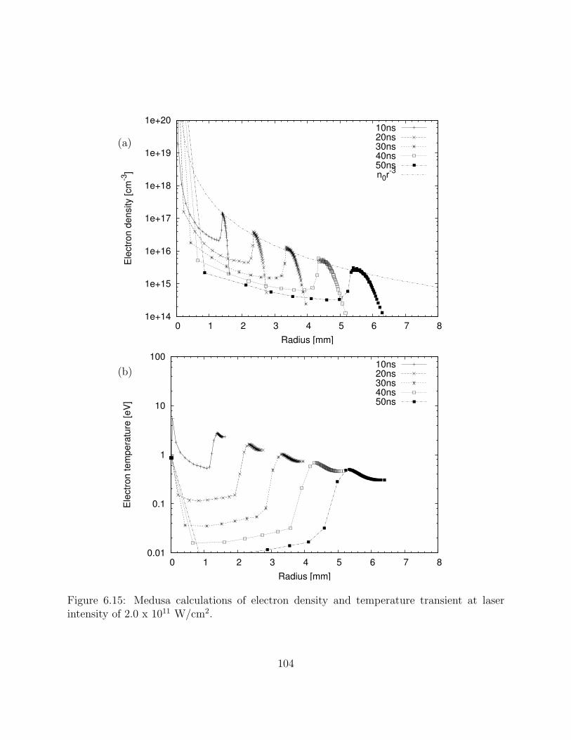
1e+14
1e+15
1e+16
1e+17
1e+18
1e+19
1e+20
0 1 2 3 4 5 6 7 8
Ele
ctro
n de
nsity
[cm
-3]
Radius [mm]
10ns20ns30ns40ns50nsn0r-3
0.01
0.1
1
10
100
0 1 2 3 4 5 6 7 8
Ele
ctro
n te
mpe
ratu
re [e
V]
Radius [mm]
10ns20ns30ns40ns50ns
Figure 6.15: Medusa calculations of electron density and temperature transient at laserintensity of 2.0 x 10¹¹ W/cm2.
(a)
(b)
104
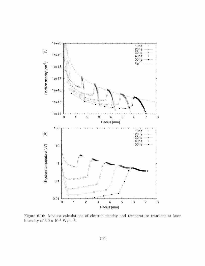
1e+14
1e+15
1e+16
1e+17
1e+18
1e+19
1e+20
0 1 2 3 4 5 6 7 8
Ele
ctro
n de
nsity
[cm
-3]
Radius [mm]
10ns20ns30ns40ns50nsn0r-3
0.01
0.1
1
10
100
0 1 2 3 4 5 6 7 8
Ele
ctro
n te
mpe
ratu
re [e
V]
Radius [mm]
10ns20ns30ns40ns50ns
Figure 6.16: Medusa calculations of electron density and temperature transient at laserintensity of 3.0 x 10¹¹ W/cm2.
(a)
(b)
105

6.4.3 Comparison between simulations and ion measurements
As calculated previously the high electron temperature region propagates as the
plasma expands. This region contains more electrons, which are equal to the charge carried
by ions, than the lower temperature plasma region. Comparison between the ion probe
signals and the density transients are made. Figure 6.17 shows IP signals and electron
density transients at the distance of the IP. The IP signals show the ion flux transients at a
distance of 10 cm from the source. Due to the discrete positions of the cells in the simulation,
the density transient is less accurate. The density value is averaged over the distance of 99.75
mm to 100.25 mm. The calculation extends to more than 1 µs after the laser pulse peak so
that the electron density peak propagates to a distance of more than 10 cm.
The TOFs of the peaks from the IP signals have good agreement with the electron
density transients. The high peaks observed in IP for all the measurements are the result
of detecting this high density region. Whereas, the electron density transients show little
signal in the tail after the peaks. This is caused by the approximation of the mass of the
ions which is made in the simulation. The averaged ion expansion is more uniform than the
mixture of different masses. The masses of atoms in the target range from 1 A.M.U. to 119
A.M.U. This is confirmed by reconstructing the IP signals from ion energy spectra.
The ion signal reconstruction can be made from ion kinetic energy distributions. The
ion signals are calculated in terms of the charge carried by specific ion species at a given
TOF. The total ion signals of different elements and the overall ion signals are calculated as
the summations of each ion signal. Figure 6.18 (a) and (b) show that the total signals consist
of all different elements in the target. It is clear that lighter ions dominate at the beginning
of the IP signal and the heaviest ions, tin ions, dominate the tail of the IP signal. This trend
is more prominent in the ion signals obtained for plasma at higher laser intensities.
106
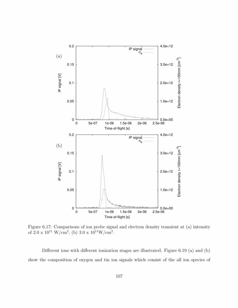
0
0.05
0.1
0.15
0.2
0 5e-07 1e-06 1.5e-06 2e-06 2.5e-060.0e+00
1.0e+12
2.0e+12
3.0e+12
4.0e+12
IP s
igna
l [V
]
Ele
ctro
n de
nsity
r=10
0mm
[cm
-3]
Time-of-flight [s]
IP signalne
0
0.05
0.1
0.15
0.2
0 5e-07 1e-06 1.5e-06 2e-06 2.5e-060.0e+00
1.0e+12
2.0e+12
3.0e+12
4.0e+12
IP s
igna
l [V
]
Ele
ctro
n de
nsity
r=10
0mm
[cm
-3]
Time-of-flight [s]
IP signalne
Figure 6.17: Comparisons of ion probe signal and electron density transient at (a) intensityof 2.0 x 10¹¹ W/cm2, (b) 3.0 x 10¹¹W/cm2.
(a)
(b)
Different ions with different ionization stages are illustrated. Figure 6.19 (a) and (b)
show the composition of oxygen and tin ion signals which consist of the all ion species of
107
different ionization stages. The laser intensity is 2.8 x 10¹¹ W/cm2 which is slightly higher
than the intensity for the optimum CE, but, they illustrate well the composition of ion
signals of different ionization stages. The ion signals of higher ionization stages O5+ and
Sn5+, have peaks at the beginning of the IP signals. The signals from low ionization stages,
Sn2+, have long tails. This difference in the ionization stages in two different density regions
is due to different recombination rates. As seen in Equation 2.16 and as discussed previously,
the rate is lower in the higher temperature region than the lower temperature region. The
higher ionization stages are the result of lowered recombination processes in the expanding
plasma. The kinetic energies of the ions with high ionization stages are high and they have
population peaks at high energy regions as seen previously.
By comparing the signal profiles of reconstructed ion signals to the measured IP
signals, shown in Figure 6.18, it is clearly seen that the spectrometer measurements preserve
the details of the ion species. The ion flux limiting aperture of the ion spectrometer is at
a distance of 10 cm from the plasma source which is the typical distance of the ion probe.
The spectrometer measures the same ion flux as ion probe even though the ion detector of
the spectrometer is placed at a distance of 90 cm from the plasma in a separate vacuum
chamber. This comparison asserts the validity of ion energy distributions measured by the
ion spectrometer.
108

0
0.005
0.01
0.015
0.02
0 5e-07 1e-06 1.5e-06 2e-06 2.5e-06 3e-06
Ion
flux
[A/s
r]
Time-of-flight [s]
TOF signal composition 1.9 x 10¹¹ W/cm2
TotalTotal HTotal OTotal Cl
Total Sn
0
0.005
0.01
0.015
0.02
0.025
0.03
0.035
0.04
0 5e-07 1e-06 1.5e-06 2e-06 2.5e-06 3e-06
Ion
flux
[A/s
r]
Time-of-flight [s]
TOF signal composition 2.8 x 10¹¹ W/cm2
TotalTotal HTotal OTotal Cl
Total Sn
Figure 6.18: Reconstructed ion signals of total signals and individual elements at laserintensities of (a) 1.9 x 10¹¹, (b) 2.8 x 10¹¹ W/cm2.
(a)
(b)
109

0
0.005
0.01
0.015
0.02
0.025
0.03
0 5e-07 1e-06 1.5e-06 2e-06 2.5e-06 3e-06
Ion
flux
[A/s
r]
Time-of-flight [s]
TOF signal composition 2.8 x 10¹¹ W/cm2
Total OO+
O2+
O3+
O4+
O5+
0
0.002
0.004
0.006
0.008
0.01
0 5e-07 1e-06 1.5e-06 2e-06 2.5e-06 3e-06
Ion
flux
[A/s
r]
Time-of-flight [s]
TOF signal composition 2.8 x 10¹¹ W/cm2
Total SnSn+
Sn2+
Sn3+
Sn4+
Sn5+
Figure 6.19: Reconstructed ion signals at laser intensities of 2.8 x 10¹¹ W/cm2. (a) Oxygenions, and (b) tin ions
(a)
(b)
110

6.5 Summary of ion emission characteristics
Ion emissions from tin-doped droplet plasmas are characterized and the ion flux
for different tin concentrations and different laser intensities are obtained. The plasma
expansion velocities increase about 50 % as the laser intensity is increased by 3 times the
intensity for the optimum CE. Quantitative ion spectrometer analysis is made and the all
ion energy distributions at different laser intensities are obtained. Large populations of low
energy and ions with low ionization stages are observed. The energy distributions are used
to estimate the collector mirror lifetime. The lifetime is about a factor of 500 shorter than
the EUVL roadmap requirement without any mitigation applied. Small populations of high
energy ions with high ionization stages are also observed. Further analysis on IP and ESIEA
measurements compared to fluid simulations shows good agreement between the two. The
ions with the high ionization stages are preserved in the high electron temperature region in
the expanding plasma under low recombination conditions.
111

CHAPTER 7
MITIGATION
7.1 Introduction
Mitigation, or ”inhibition” in a general sense, is the prevention of particles from
reaching the collection optics. The term ”particles” as used in this chapter is considered to
be any form of ejected target material during plasma production causing mirror reflectiv-
ity degradation. These include aerosols, neutral atoms, clusters, and ions. All mitigation
schemes must not absorb or block useful EUV radiation while they are required to stop, slow
down, or repel particles. The mitigation schemes that are investigated extensively in this
study are an electrostatic field mitigation scheme, called the Repeller Field, and a Magnetic
Foil Trap where a magnetic field is implemented.
7.1.1 Types of mitigation schemes
Many mitigation schemes have been proposed by different research groups in the
EUVL source development community. The essential function of mitigation is to reduce the
momentum of the particles. One common mitigation scheme is the use of a buffer gas. This
mitigation scheme can be realized by just filling buffer gases [95] in the vacuum chamber
or making a localized volume with buffer gas referred to as a gas curtain or gas flow [96].
The gases can be ionized to improve the interaction between ions and electrons of the source
plasma and those generated in the buffer gases. The ionized gases that have been proposed
are secondary plasma [97] and secondary plasma shutter [98]. The particles straggle and
112
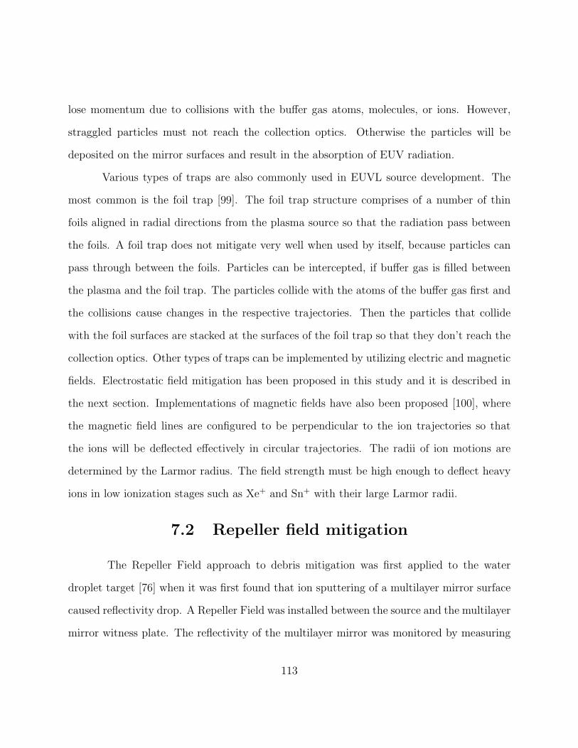
lose momentum due to collisions with the buffer gas atoms, molecules, or ions. However,
straggled particles must not reach the collection optics. Otherwise the particles will be
deposited on the mirror surfaces and result in the absorption of EUV radiation.
Various types of traps are also commonly used in EUVL source development. The
most common is the foil trap [99]. The foil trap structure comprises of a number of thin
foils aligned in radial directions from the plasma source so that the radiation pass between
the foils. A foil trap does not mitigate very well when used by itself, because particles can
pass through between the foils. Particles can be intercepted, if buffer gas is filled between
the plasma and the foil trap. The particles collide with the atoms of the buffer gas first and
the collisions cause changes in the respective trajectories. Then the particles that collide
with the foil surfaces are stacked at the surfaces of the foil trap so that they don’t reach the
collection optics. Other types of traps can be implemented by utilizing electric and magnetic
fields. Electrostatic field mitigation has been proposed in this study and it is described in
the next section. Implementations of magnetic fields have also been proposed [100], where
the magnetic field lines are configured to be perpendicular to the ion trajectories so that
the ions will be deflected effectively in circular trajectories. The radii of ion motions are
determined by the Larmor radius. The field strength must be high enough to deflect heavy
ions in low ionization stages such as Xe+ and Sn+ with their large Larmor radii.
7.2 Repeller field mitigation
The Repeller Field approach to debris mitigation was first applied to the water
droplet target [76] when it was first found that ion sputtering of a multilayer mirror surface
caused reflectivity drop. A Repeller Field was installed between the source and the multilayer
mirror witness plate. The reflectivity of the multilayer mirror was monitored by measuring
113

the EUV emission from the source. The reflectivity lifetime was extended by factor of ∼ 10
with the Repeller Field use. From this result it can be concluded that the field reduced ion
flux.
The Repeller Field concept was applied to the tin-doped droplet target as well [91].
The effectiveness of the Repeller Field was evaluated in terms of reduction of the tin aerosol
flux. Two witness samples were exposed to the plasma, one with the field applied and another
without the field. The amount of tin deposition on the witness plate which was exposed with
the Repeller Field was less than that on the plate without the field. The result showed that
the field reduced the aerosol flux. These two early results lead to the more detailed analysis
on the Repeller Field effectiveness for both ion flux and aerosol flux, which is described in
the following two sections.
7.2.1 Effectiveness of repeller field on ion flux
The Repeller Field is found to be capable of extending the mirror lifetime by reducing
ion flux but the details of the reduction process are still unknown. It is possible to obtain
detailed effectiveness of Repeller Field on ion flux by utilizing the ion diagnostics that are
described in previous chapter. Ion probes (IP) and electrostatic ion energy analyzer (ESIEA)
are applied to evaluate the effect of Repeller Field on ion flux.
One of the results from the IP measurements is shown in Figure 7.1. The comparison
indicates the reduction of the ion flux at the beginning of the signal. In the IP signal with
no field applied, the fastest ions appear as a step or a shoulder, which is not observed when
the field is applied. It is seen repeatedly by switching on and off the voltage supply. The
reduced ion flux is from hydrogen ions, protons, based on the lighter mass than the oxygen’s.
However, the reduction is the only apparent difference in the comparison. Once the high
114
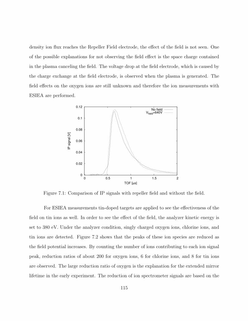
density ion flux reaches the Repeller Field electrode, the effect of the field is not seen. One
of the possible explanations for not observing the field effect is the space charge contained
in the plasma canceling the field. The voltage drop at the field electrode, which is caused by
the charge exchange at the field electrode, is observed when the plasma is generated. The
field effects on the oxygen ions are still unknown and therefore the ion measurements with
ESIEA are performed.
0
0.02
0.04
0.06
0.08
0.1
0.12
0 0.5 1 1.5 2
IP s
igna
l [V
]
TOF [µs]
No fieldVfield=640V
Figure 7.1: Comparison of IP signals with repeller field and without the field.
For ESIEA measurements tin-doped targets are applied to see the effectiveness of the
field on tin ions as well. In order to see the effect of the field, the analyzer kinetic energy is
set to 380 eV. Under the analyzer condition, singly charged oxygen ions, chlorine ions, and
tin ions are detected. Figure 7.2 shows that the peaks of these ion species are reduced as
the field potential increases. By counting the number of ions contributing to each ion signal
peak, reduction ratios of about 200 for oxygen ions, 6 for chlorine ions, and 8 for tin ions
are observed. The large reduction ratio of oxygen is the explanation for the extended mirror
lifetime in the early experiment. The reduction of ion spectrometer signals are based on the
115

kinetic energy distributions of individual ion species. The ions detected by the spectrometer
have reduced kinetic energies of 380 eV after the Repeller Field. They originally have higher
kinetic energies. The chlorine and tin ion species have more populations in higher kinetic
energy distribution due to their higher mass than oxygen’s. Higher field potential can reduce
the kinetic energy of these Cl and Sn ions. Currently, the voltage applied is the maximum
without having discharge between the electrode and other components in the chamber. To
reduce ion flux of tin ions, more effective schemes are necessary. The Magnetic Foil Trap
mitigation is discussed later in this chapter in terms of high energy tin ions.
116
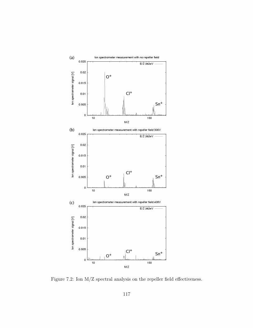
Figure 7.2: Ion M/Z spectral analysis on the repeller field effectiveness.
117

7.2.2 Effectiveness of repeller field on aerosols
It is seen that Repeller Field reduces the aerosol flux which is described in the
following sections. This is important in cases where the droplet target positioning is unstable
resulting in insufficient heating. When the droplet target is not placed at the desired position
in the laser focus, a part of or the entire target is not heated as expected. As a result, a large
number of aerosols are created. However, the aerosols that are created in the plasma are
charged by the plasma potential [101]. Therefore, it is possible to repel the charged aerosols
by the Repeller Field.
Two witness plates are exposed to the plasma source, one with the field applied and
the other with no field applied. The amount of the tin deposits on the two samples is
compared with the help of Auger electron spectroscopy (AES). Figure 7.3 shows the images
of the two witness plates (Si wafer) with surfaces area of 50µm x 50µm, after 3 x 10⁴ laser
shots, where the distance from the source is 64 mm. Figure 7.3 (a) and (b) are images of the
secondary electron images obtained using AES and (c) and (d) are the elemental mapping
of the tin signal from the same areas of (a) and (b), respectively. The reduction ratio can
be obtained by either counting the number of deposits or calculating the fraction of area
covered by the deposits. The numbers of deposits on the samples are 152 and 41 for (a) and
(b) respectively. The reduction ratio is 3.7. The fraction of surface coverage is reduced from
65 % to 10 %, where the reduction ratio is 6.5. Due to the fact that aerosols are produced
during the source plasma generation, they are charged. The mass to charge ratio depends
on the surface area and the mass. It tends to be difficult to mitigate large aerosols which are
likely to have large mass to charge ratio. However, the aerosol generation can be controlled
by optimizing the laser irradiation conditions, as described in Chapter 5.
118

(a) (b)
(c) (d)
Figure 7.3: (a) Secondary electron image of 50µm x 50µm of surface exposed without therepeller field, (b) Secondary electron image of 50µm x 50µm of surface exposed with therepeller field, (c) Auger electron tin elemental mapping of the same area as (a), (d) Tinelemental mapping of the same area as (b).
119
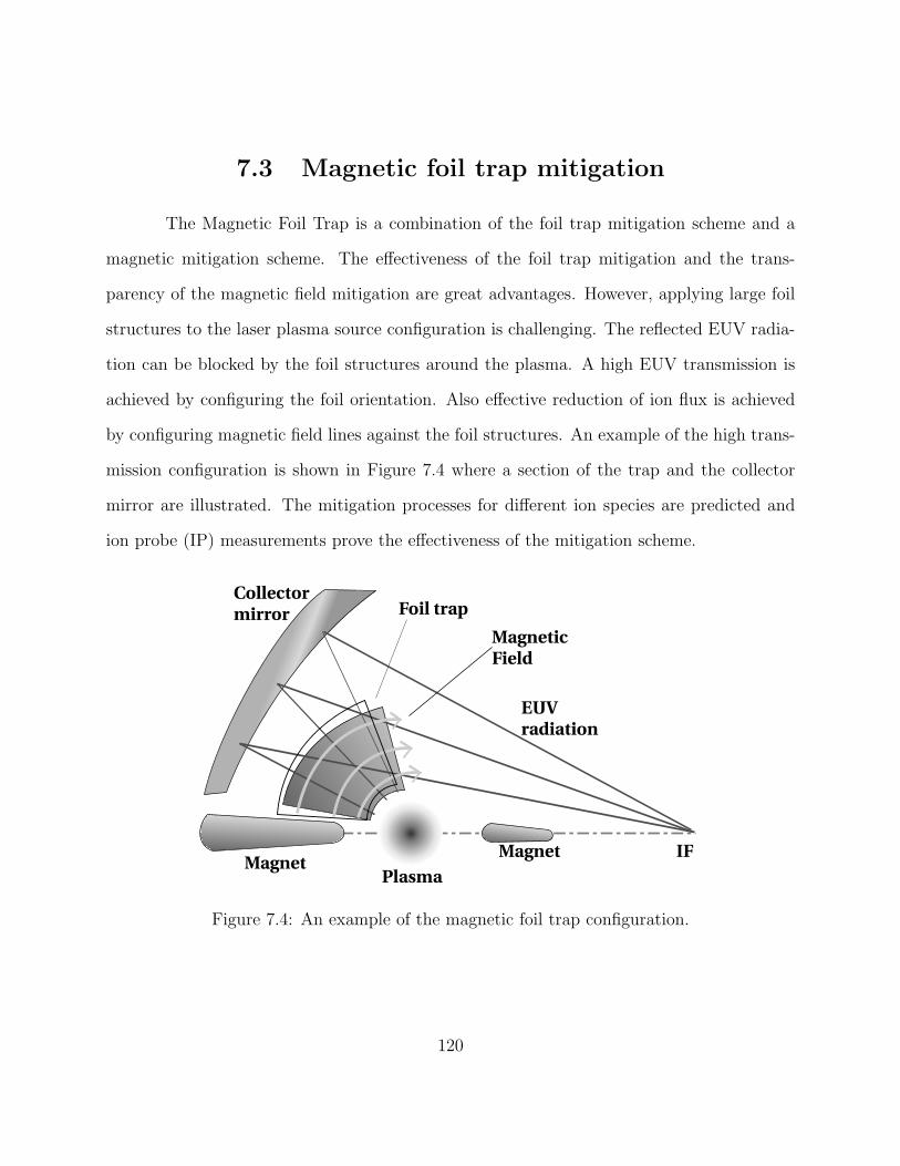
7.3 Magnetic foil trap mitigation
The Magnetic Foil Trap is a combination of the foil trap mitigation scheme and a
magnetic mitigation scheme. The effectiveness of the foil trap mitigation and the trans-
parency of the magnetic field mitigation are great advantages. However, applying large foil
structures to the laser plasma source configuration is challenging. The reflected EUV radia-
tion can be blocked by the foil structures around the plasma. A high EUV transmission is
achieved by configuring the foil orientation. Also effective reduction of ion flux is achieved
by configuring magnetic field lines against the foil structures. An example of the high trans-
mission configuration is shown in Figure 7.4 where a section of the trap and the collector
mirror are illustrated. The mitigation processes for different ion species are predicted and
ion probe (IP) measurements prove the effectiveness of the mitigation scheme.
Plasm a
Colle ctorm irror
M agne ticFie ld
EU Vradiation
IF
Foil trap
M agne tM agne t
Figure 7.4: An example of the magnetic foil trap configuration.
120
7.3.1 Particle motion in the magnetic field and foil structures
The motion of a charged particle in a magnetic field is described by the Newtonian
equation with the Lorentz force,
m~a = q(~v × ~B) (7.1)
where a is the acceleration of the particle, q is the charge of the particle, v is the velocity of
the particle and B is the magnetic field. By solving Equation 7.1, the particle motion and
the position of the particle as function of time is obtained. In a uniform magnetic field, the
motion is a circular motion whose radius is the Larmor radius expressed in,
rL =mv
qB(7.2)
The orbit of charged high Z material under a typical magnetic field as for instance that
obtained from a permanent magnet, is usually large when compared to the size of the foil
trap or the source-mirror distances. For example, a singly ionized tin ion with kinetic energy
of 1 keV has a radius of 50 cm under a uniform magnetic field of 0.1 T. The ion energy
distribution shows that ions with even higher energies are generated. A magnetic field of at
least 2 T is necessary to make a circular motion with 10 cm diameter for 4 keV Sn+ ions.
It is not realistic to have uniform, high magnetic fields in a large area without blocking the
EUV radiation. The Magnetic Foil Trap mitigation scheme utilizes magnetic fields which can
be obtained from commercially available permanent magnets. The magnetic field is locally
applied in the vacuum space around the source plasma. In such a magnetic field, the motions
of the particles are arcs between the source and the mirror.
The deflection of the particle and the foil trap configuration are considered. When a
trajectory of a particle is intercepted by a foil surface, the particle is trapped. Let Φ be the
deflection angle in radians. The distance or radius of the particle position from the source
121

is R in meters. Some relationships of Φ and R are shown in Figure 7.5. The trajectories
of Sn2+ or Sn+ with kinetic energies of 500 eV and 1000 eV are calculated under uniform
magnetic field of 0.1 T to illustrate the relationship between Φ and R. The curves in Figure
7.5 can be approximated in linear relationship with a constant slope of Φ/R. The value,
Φ/R, represents the deflection rate. Because the deflection rate is nearly constant over a
few cm to a few tenths of a cm, the foil trap design criteria can be simplified. Figure 7.5
illustrates the critical ion trajectory with a foil configuration where the ion barely passes
through the trap. The kinetic energy of the ion will be the cut off energy of the foil trap.
Any ions with smaller kinetic energies than the cut off energy will be deflected more, and
thus they will be trapped. In contrast, an ion with higher kinetic energy than the cut off
energy will have a smaller deflection rate and it will not be trapped. The cut off energy
is determined by the geometry of the foil configuration. The relationship between the foil
angle Φfoil and the foil radius Rfoil is expressed in,
Φfoil
Rfoil
=Φout − Φin
Rout −Rin
(7.3)
where the Φin, Φout, Rin, Rout are shown in Figure 7.6. To determine if any ion species are
trapped or not trapped by the foil structure, the calculated deflection rate Φ/R is compared
to the Φfoil/Rfoil.
Figure 7.7 shows the deflection rates calculated for several cases. Figure 7.7 (a)
illustrates the deflection rates of different ion species where larger mass charge ratio of a
singly charged tin ion is most unlikely to be deflected. Figure 7.7 (b) shows exactly the
same characteristics with different ion species. With the magnetic field of 0.1 T the foil
trap configuration has to have small enough Φfoil/Rfoil to trap high energy Sn+ ions. The
calculated Φ/R of Sn+ ion with kinetic energy of 10 keV is about 0.3 rad/m. For example a
foil trap configuration with a foil angle of 0.03 rad, a foil inner radius of 2 cm, and a foil outer
122

radius of 12 cm could trap high energy Sn+ ions of up to 10 keV. In such a configuration,
there will be more than 100 foils over a hemisphere. The obscuration of such a trap can be
significant due to the large number of foils. Figure 7.7 (c) shows that the number of foils
can be reduced by increasing the magnetic field strength. Under increased magnetic field,
for instance 0.5 T, Φ/R of Sn+ ion with kinetic energy of 10 keV is about 1.6 rad/m. With
the same radii for the foils in the previous example, foil angle can be relaxed to 0.16 rad.
There will be only 20 foils in a hemisphere to trap all of the Sn+ ions with kinetic energies
up to 10 keV. In reality, a magnetic field is not uniform over a large area. Once the magnetic
field profile is measured, ion trajectories can be calculated as well as deflection rates. The
foil angle can then be determined by the deflection rate as described above.
123

0
0.1
0.2
0.3
0.4
0.5
0.6
0.7
0 0.1 0.2 0.3 0.4 0.5
φ [ra
d]
R [m]
Sn+ 500eVSn+ 1000eVSn2+ 500eV
Sn2+ 1000eV
Figure 7.5: Relationships between Φ and R under a uniform magnetic field.
R
in
R
out
Φin
Φout
F
o
i
l
P
l
a
n
e
s
Critical Ion
Trajectory
Plasm a
Source
Figure 7.6: The illustration of the critical ion trajectory and foils.
124

0
0.5
1
1.5
2
2.5
3
3.5
4
4.5
0 2 4 6 8 10
φ/R
[rad
/m]
Ion kinetic energy [keV]
Sn+ Sn2+
Sn3+
0
0.5
1
1.5
2
2.5
3
3.5
4
0 2 4 6 8 10
φ/R
[rad
/m]
Ion kinetic energy [keV]
O+
Cl+Sn+
0
1
2
3
4
5
6
7
8
0 2 4 6 8 10
φ/R
[rad
/m]
Ion kinetic energy [keV]
0.1T0.2T0.5T
Figure 7.7: Ion deflection rates of (a) tin ion species under uniform magnetic field of 0.1T (b) different ion species under uniform magnetic field of 0.1 T (c) Sn+ under differentmagnetic field.
(a)
(b)
(c)
125

7.3.2 Particle motion in non-uniform magnetic field
The magnetic field of the magnetic core described in Figure 4.14 is measured, and
the result is shown by Figure 7.8. The pair of foils are perpendicular to the axis of two
magnets. The magnetic field measured at the foil axis is used to calculate trajectories of
different ion species. Any charged particle motion in a magnetic field can be calculated by
the Newtonian equation described by 7.1. In each local point a uniform magnetic field is
assumed and in such case the trajectory calculation is completed in exactly the same manner
as described in the previous section. In finite time durations an ion experiences a Lorentz
force which produces an acceleration of the ion. The acceleration changes the velocity with
the finite time duration. A series of calculations provide the total trajectory of an ion with
any given kinetic energy and mass-charge ratio.
It is difficult to trap ion species with large mass-charge ratio. In the tin-doped droplet
target case, it is Sn+. The deflection rate for this ion, with a kinetic energy of 1.5 keV, is
0.9 rad/m. For a foil angle of 0.1 rad and foil length of 0.1 m, the ion can go through
the Magnetic Foil Trap. However, it is expected that most of the oxygen ions with kinetic
energies of up to 7 keV will be trapped. There is a maximum to the ion energy in trapping
ions. The kinetic energy is the cut off energy. The effectiveness of the mitigation schemes is
evaluated with the predicted cut off energies.
126
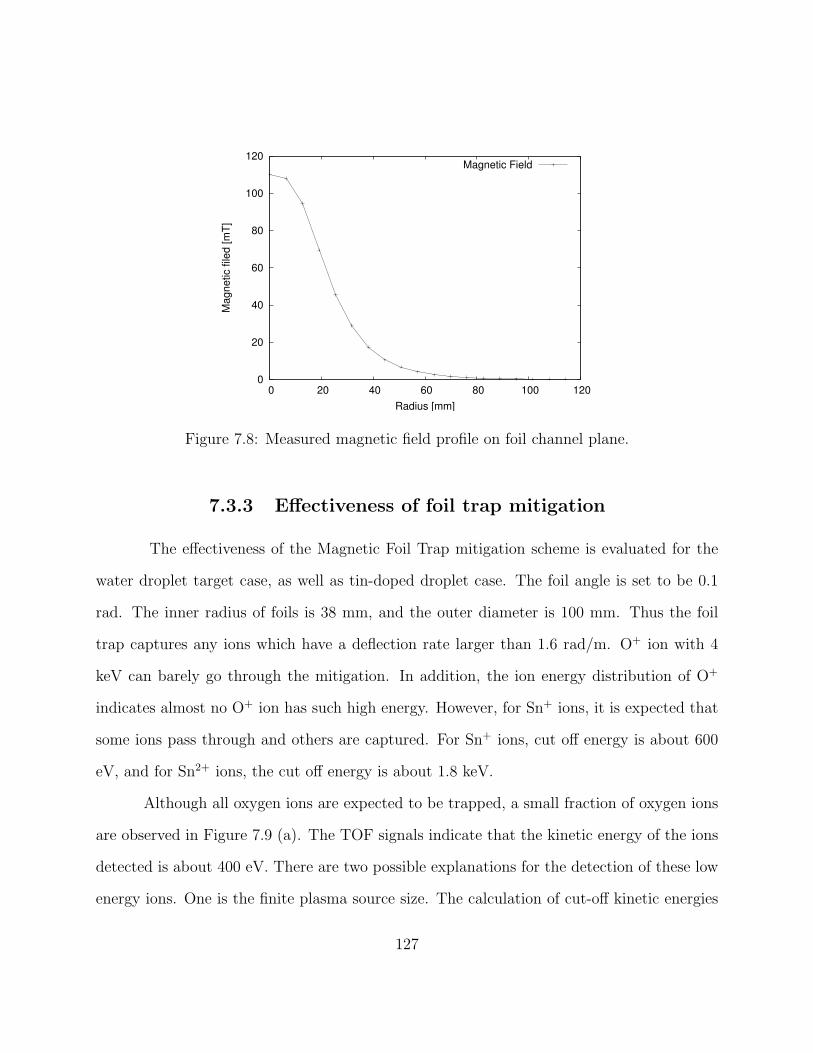
0
20
40
60
80
100
120
0 20 40 60 80 100 120
Mag
netic
file
d [m
T]
Radius [mm]
Magnetic Field
Figure 7.8: Measured magnetic field profile on foil channel plane.
7.3.3 Effectiveness of foil trap mitigation
The effectiveness of the Magnetic Foil Trap mitigation scheme is evaluated for the
water droplet target case, as well as tin-doped droplet case. The foil angle is set to be 0.1
rad. The inner radius of foils is 38 mm, and the outer diameter is 100 mm. Thus the foil
trap captures any ions which have a deflection rate larger than 1.6 rad/m. O+ ion with 4
keV can barely go through the mitigation. In addition, the ion energy distribution of O+
indicates almost no O+ ion has such high energy. However, for Sn+ ions, it is expected that
some ions pass through and others are captured. For Sn+ ions, cut off energy is about 600
eV, and for Sn2+ ions, the cut off energy is about 1.8 keV.
Although all oxygen ions are expected to be trapped, a small fraction of oxygen ions
are observed in Figure 7.9 (a). The TOF signals indicate that the kinetic energy of the ions
detected is about 400 eV. There are two possible explanations for the detection of these low
energy ions. One is the finite plasma source size. The calculation of cut-off kinetic energies
127

assumes a point source for the ion generation. Another is the scattering of ions. While the
plasma is expanding from the hot dense plasma phase, highly charged ion collisions can add
slight deflection to the trajectories.
0
0.005
0.01
0.015
0.02
0.025
0.03
0.035
0.04
0 5e-07 1e-06 1.5e-06 2e-06 2.5e-06 3e-06 3.5e-06
Ion
prob
e si
gnal
[V]
Time-of-flight [s]
+Foil+Foil+MField
0
0.005
0.01
0.015
0.02
0.025
0.03
0 1e-06 2e-06 3e-06 4e-06 5e-06
Ion
prob
e si
gnal
[V]
Time-of-flight [s]
+Foil+Foil+MField
Figure 7.9: IP measurement with magnetic foil trap for (a) water droplet target case, (b)tin-doped droplet target case.
(a)
(b)
128

As expected previously, higher energy tin ions are detected as shown in Figure 7.9
(b). The small signal peak with mitigation gives TOF signal measurements of about 1.6 µs,
which corresponds to a kinetic energy of 2 keV. Low signal amplitude of scattering ions is
also detected. The reduction factors for the two different targets are 20 for water droplet,
and 6.5 for tin-doped droplet target, which are calculated by integrating the area of these
signals. Higher reduction ratios can be obtained by configuring a small deflection angle, in
other words, a smaller foil angle and/or large distance between the inner radius and outer
radius of the foil. It can also be obtained by increasing the magnetic field.
7.4 Combination of two mitigation schemes
In order for tin-doped droplet targets to satisfy the EUVL source lifetime require-
ment, a large factor of ion flux reduction is necessary. As described in the previous chapter,
the lifetime requirement must be met with a reduction in ion flux of at least 500. The factors
of reductions of Repeller Field and Magnetic Foil Trap each range from 5 to 20. When the
two mitigation schemes are combined together, it is expected that the reduction factor will
be around a hundred. Further reduction can be achieved with minor modifications to both
schemes. However, detecting reduced ion flux becomes difficult. As demonstrated in the
following sections, IP is not sensitive enough to detect reduced ion flux. Instead, a channel
electron multiplier is utilized to realize an amplified ion probe. It is discussed in the later
section that the ion flux reduction that is obtained with combined mitigation schemes is
sufficient to satisfy the lifetime requirement.
129

7.4.1 Detection limit of ion flux
Here an improved ion mitigation is described when the Repeller Field is modified to
have higher voltage driving capacity. A power supply that can provide higher voltage and
higher current is used. The field electrode is encapsulated to reduce discharge between high
voltage electrodes and other components in the vacuum chamber. It is isolated with a PVC
tube and has ground electrodes, as shown in Figure 7.10. The electric field is principally
contained to between the ground electrodes. With short distances between the ground
electrodes and the high voltage electrode, a higher breakdown voltage is expected due to the
concept of Paschen’s law [102].
Figure 7.10: Photo and schematic of modified encapsulated repeller field mitigation.
130

Ion probe measurements were carried out with this modified Repeller Field for water
droplet targets. The laser intensities for this measurement, for the modified Magnetic Foil
Trap, and the combination of two mitigation schemes are around 3 x 10¹¹ W/cm2. These
intensities were too high to have the highest CE. However, the generation of higher energy
ions is preferred for evaluating the effectiveness of the schemes. Figure 7.11 shows improved
reduction compared to the previous configuration which is shown in Figure 7.1. Higher ion
flux can be reduced by a factor of about four. This modified Repeller Field is used with
another modified magnetic foil mitigation.
A new configuration of the Magnetic Foil Trap was applied with a smaller deflection
rate of 0.5 rad/m. The foil angle was 0.05 rad, and the distance between the inner radius
and the outer radius is 10 cm. The magnetic field itself was unchanged. The cut off energy
for Sn+ was 5 keV, and for Sn2+ was 20 keV. IP measurements were carried out with the
modified Magnetic Foil Trap for tin-doped droplet targets which is shown in Figure 7.12. A
large reduction in ion flux was observed. Peaks caused by higher energy tin ions were not
observed by IP. However the signal level was close to the minimum detection level of IP and
the oscilloscope. Therefore the amplified ion probe is utilized.
131

0
0.0002
0.0004
0.0006
0.0008
0.001
0.0012
0 1e-06 2e-06 3e-06 4e-06 5e-06
Ion
prob
e si
gnal
[v]
Time-of-flight [s]
Ion probe signals
No magnetic field+Repeller field 1.3 kV+Repeller field 1.7 kV
Figure 7.11: IP signal comparison between different field potentials of the modified RepellerField.
0
0.0005
0.001
0.0015
0.002
0.0025
0.003
0.0035
0.004
0 1e-06 2e-06 3e-06 4e-06 5e-06
Ion
prob
e si
gnal
[v]
Time-of-flight [s]
No magnetic field+Magnetic field
Figure 7.12: IP signals on the modified Magnetic Foil Trap.
132

7.4.2 Demonstration of sufficient ion flux reduction
The ion flux is measured by the amplified ion probe described in Figure 4.10. Three
ion signals, with no mitigation but a foil trap, with foil trap and magnetic field, and with
Magnetic Foil Trap and Repeller Field are compared in Figure 7.13. The signals are amplified
by a factor of 107 with a -3 kV bias. The ion signal with the foil trap shows a dip at 2.3 µs.
The ion flux would be highest where the dip is, according to all the previous measurements.
The amplified ion signals can be suppressed by gain reduction due to excess instant signal
current and detection efficiency reduction with too high ion density at the detector surface.
The dip appears regardless of the biasing voltage. Thus the ion flux is too high with the
limiting aperture of 2 mm and the CEM distance from the plasma. However, detection levels
of the ion flux are barely adequate when mitigation schemes are installed. Very low ion flux
is measured with mitigation schemes. The remaining ion signals only have a small peak
when mitigation schemes are installed. The corresponding ion kinetic energy is about 10
keV for tin ions. It can be further reduced by increasing the magnetic field.
-0.02
-0.015
-0.01
-0.005
0
0.005
0 1e-06 2e-06 3e-06 4e-06 5e-06 6e-06 7e-06 8e-06
CE
M s
igna
l [v]
Time-of-flight [s]
+Foil+Magnetic field
+MF + Repeller field 600 V
Figure 7.13: Amplified ion probe signals with two mitigation schemes installed.
133

With the combined mitigation configuration of modified Repeller Field and Magnetic
Foil Trap, the erosion rate is calculated based on the ion energy distributions. Although
sputtering yield for higher incident tin ions is high, the populations of these high energy ions
are very small. The lifetime estimations which are described in Chapter 6 are applied here
as well. The estimated erosion rate is 7.7 x 10¹⁰ shots for 1 nm sputtering of Si, and 6.5 x
1010 shots for 1 nm sputtering of Mo. Based on these values, 5.0 x 10¹¹ shots will be needed
to remove one layer pair Thus, the mirror reflectivity lifetime will be 7.5 x 10¹² shots, which
is equivalent to the time duration of 30,000 hours at 70 kHz source operation. It is enough
to satisfy the EUVL source lifetime.
7.4.3 Neutral atom mitigation
One insight gained by the measurements described in the previous section is that
there is no signal detected from the neutral atom flux. The CEM can detect neutral atoms.
The Repeller Field cannot manipulate neutral atoms. As plasma expands and cools down,
the ionization stages decrease. The kinetic energies of neutrals would be similar to that of
singly charged tin ions. Thus, the high-energy ion signal is not likely due to neutrals. The
whole target is ionized by the laser pulse and ions are deflected by the magnetic field of
the mitigation. When singly charged ions are recombined with electrons, they are already
deflected enough so that they are trapped by the foil surfaces. Therefore, the Magnetic Foil
Trap demonstrated mitigation effects on neutral atoms.
7.5 Summary of mitigation
The Repeller Field and Magnetic Foil Trap mitigation schemes are evaluated in
terms of both ion flux and aerosol flux. The Repeller Field reduces aerosol flux effectively,
134
but reduces ion flux less effectively. The charges in the plasma can easily cancel the field. If
the field is encapsulated so that a higher voltage can be applied, ion reduction is improved.
The Magnetic Foil Trap mitigation reduces ion flux very effectively but passes a small amount
of scattered ions. The two mitigations are combined in order to be more effective for ion
flux reduction. Only a small amount of high energy tin ions, more than 10 keV, can pass
through the two mitigation schemes. The estimated erosion rate is small due to the small
population of the high energy ions. With the implementation of the two methods described,
it is concluded that the multilayer mirror lifetime can be extended to meet the EUVL source
lifetime requirement.
135

CHAPTER 8
CONCLUSION AND FUTURE WORK
8.1 Conclusion
As described in the previous chapter, tin-doped droplet laser plasma sources can
satisfy the EUVL source lifetime requirements with the use of the two mitigation schemes
described here. A separate program demonstrated high CE [59]. The EUV power delivery
can be achieved with the use of high repetition rate lasers. Therefore, it is expected that
this target configuration will satisfy the most challenging aspects of the source requirements;
power and lifetime. To support this conclusion this study discusses the debris emission
characteristics and mitigation effectiveness. Aerosols are observed on witness plates and
identified as tin which are generated in the target under insufficient laser heating. The
generation of aerosols is minimized by optimizing the laser intensities. Ion kinetic energy
distributions for individual ion species are characterized for different laser intensities. The
distributions are used with surface sputtering simulation code to estimate the erosion rates
of multilayer mirrors. The estimated lifetime is a factor of about 500 shorter than the
requirement with no mitigation techniques applied.
Two mitigation schemes are evaluated in reducing aerosol flux and ion flux. The
combination of these two mitigation schemes demonstrated a sufficient reduction in ion flux.
This study also discusses mass limited targets, the mechanisms behind mirror degradation,
fluid properties of laser plasmas, the instrumentation for debris detection and analysis to
validate all the measurements and analysis.
136

8.2 Future work
There are some uninvestigated areas which relate to this study. One of them is a
real erosion rate measurement by exposing multilayer surfaces with long term laser plasma
source operations. Reliable angular distribution profiles of not only ion emission but also
EUV radiation are unavailable. Tin ion implantation can be possible and the impact of this
on the reflectivity lifetime is unknown. The Magnetic Foil Trap is effective in mitigating
ions, but the radiation characteristics from the plasma may be affected under the magnetic
field due to the electron cyclotron motion that tends to prohibit electron-ion collisions. The
plasma density and temperature transient can be measured and compared with predictions
by fluid simulations. It might be possible to manipulate the plasma density and temperature
before and after the targetlaser interaction in order to lower the kinetic energies transferred
to ions. These areas can be investigated with new facilities and raise other research topics
and areas. The following sections discuss some of these topics.
8.2.1 High repetition rate laser plasmas
The current experimental facility is limited by the laser repetition rate and long term
target delivery stability. Long exposure experiments are challenging because the repetition
rate of the laser available is only 100 Hz, which is the highest repetition laser system with
appropriate parameters in the laboratory. With a higher repetition rate laser system, real
time measurements of the erosion rate can be obtained.
It is meaningful not only to measure erosion rate, but also to produce high EUV
power. It is necessary to collect the emitted radiation with large solid angle mirrors to
realize an EUV light source suitable to operate with micro exposure tools. The droplet laser
137

plasma source is small and it can be considered as point source so that imaging, exposure of
materials, and microscopy can be integrated with the high power source.
8.2.2 Target stabilization systems
Even if long term operation of the current laser is possible, it still needs an operator
to control target positioning for the duration of operation. The target supply and unused
target retrieval can be solved relatively easily. However, the slow drifting of target-laser
synchronization has to be adjusted. A separate effort is made to realize an intelligent target
positioning with 3D feedback in atmosphere which can be integrated into the target chamber.
If it is integrated with a high repetition laser system, a reliable EUV light source facility will
be realized.
By doping different materials with different concentrations into the droplet target, the
radiation from the plasma can be broadened with a mixture of many spectral peaks. Different
research areas can utilize such a single source configuration. It is convenient to have a local
short wavelength light source other than the synchrotron facilities. It can also be used as a
high energy and highly charged ion source. Different from the EUVL source collector mirror
configurations, ion emissions can also be useful. The laser irradiation conditions can be
varied for such a target. By varying the laser intensity, the plasma temperature changes as
well as radiations and ionization stages. All these ideas rely on stable target positioning.
8.2.3 Radiation study under magnetic field existence
In the long history of plasma generation and confinement, different plasma properties
under magnetic fields are often observed. The collision frequency in hot dense plasma is much
higher than the electron cyclotron frequency. The effects of the magnetic field may be too
small to observe. However, the gas discharge pinch plasmas are relatively long-lived. Any
138

CE improvement with the magnetic field in laser plasmas can enable cheaper EUVL light
sources. Any radiation confinement can reduce collection angle, as well. Reducing the size
of the collector mirror can reduce the cost of EUVL sources. Utilization of grazing incidence
mirrors with confined laser plasmas may be possible.
8.2.4 Temporary and spatially resolved spectroscopy
For better understanding of the plasma physics of the droplet laser plasmas, the
combination of simulations and diagnostics are very powerful tools. The simulations are
typically bundles of calculations at different positions and different times. Most of the diag-
nostics including spectroscopy are collecting information over specific time duration. Either
temporal resolution or spatial resolution of spectroscopy can provide more detailed plasma
parameters than time and space averaged spectroscopy. The comparison between simulations
and measurements are then used to improve the plasma modeling. Improved modeling can
enhance control of experimental parameters such as laser energy, pulse duration, wavelength,
and target size.
8.2.5 Pre-pulse and post pulse heating
Pre-pulse is a small laser pulse which is applied just before the large intensity laser
pulse arrives at the target. This scheme is shown by researchers to increase CE [37, 62] as
it creates a low-density gradient plasma before the main plasma is created. The pressure
gradient produces the momentum for plasma expansion. Pressure is proportional to the
product of density and temperature. A smaller density gradient at a constant temperature
produces less momentum of expansion. Smaller expansion velocities are expected in the
presence of pre-pulse.
Similar schemes can be applied but after the laser interaction. This is a unique strat-
139

egy that can be applied with Magnetic Foil Trap mitigation. The lower electron temperature
in the majority of the plasma region after the laser pulse leads to high recombination rates.
A post pulse with a small laser energy can increase the temperature so that recombination
processes are reduced. The Magnetic Foil Trap can capture ions with higher ionization stages
easier than lower ones. Singly ionized tin ions are the most difficult to capture. Thus a post
pulse can enhance the effectiveness of the mitigation schemes.
140

APPENDIX A
ION KINETIC ENERGY DISTRIBUTIONS
141
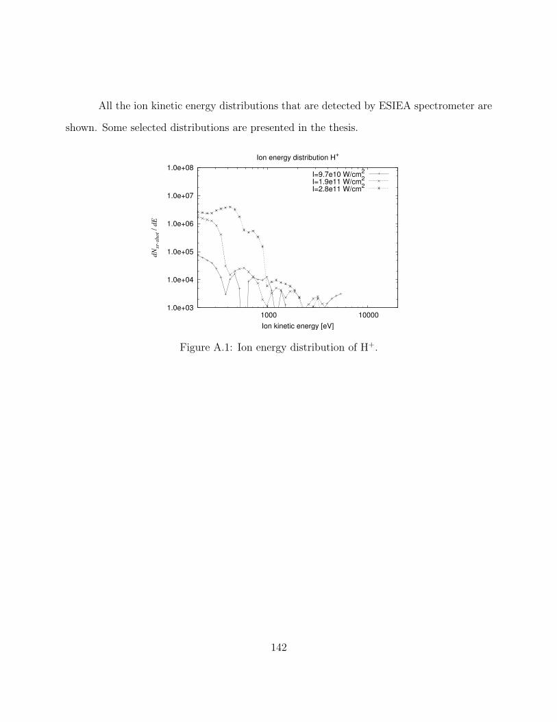
All the ion kinetic energy distributions that are detected by ESIEA spectrometer are
shown. Some selected distributions are presented in the thesis.
1.0e+03
1.0e+04
1.0e+05
1.0e+06
1.0e+07
1.0e+08
1000 10000
dNsr
-sho
t / d
E
Ion kinetic energy [eV]
Ion energy distribution H+
I=9.7e10 W/cm2
I=1.9e11 W/cm2
I=2.8e11 W/cm2
Figure A.1: Ion energy distribution of H+.
142
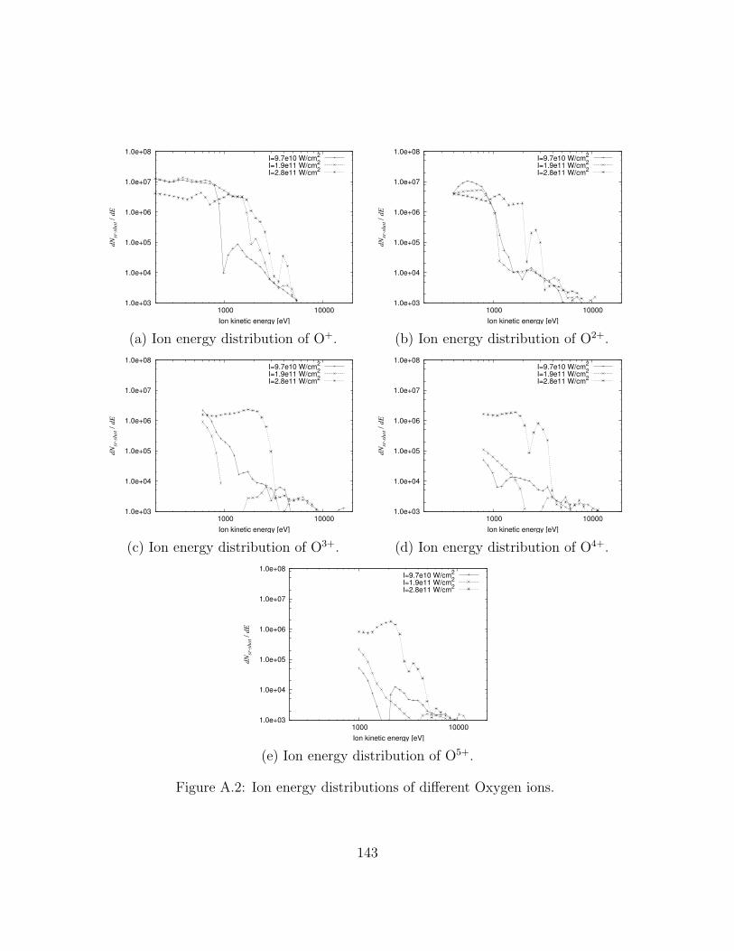
1.0e+03
1.0e+04
1.0e+05
1.0e+06
1.0e+07
1.0e+08
1000 10000
dNsr
-sho
t / d
E
Ion kinetic energy [eV]
I=9.7e10 W/cm2
I=1.9e11 W/cm2
I=2.8e11 W/cm2
(a) Ion energy distribution of O+.
1.0e+03
1.0e+04
1.0e+05
1.0e+06
1.0e+07
1.0e+08
1000 10000
dNsr
-sho
t / d
E
Ion kinetic energy [eV]
I=9.7e10 W/cm2
I=1.9e11 W/cm2
I=2.8e11 W/cm2
(b) Ion energy distribution of O2+.
1.0e+03
1.0e+04
1.0e+05
1.0e+06
1.0e+07
1.0e+08
1000 10000
dNsr
-sho
t / d
E
Ion kinetic energy [eV]
I=9.7e10 W/cm2
I=1.9e11 W/cm2
I=2.8e11 W/cm2
(c) Ion energy distribution of O3+.
1.0e+03
1.0e+04
1.0e+05
1.0e+06
1.0e+07
1.0e+08
1000 10000
dNsr
-sho
t / d
E
Ion kinetic energy [eV]
I=9.7e10 W/cm2
I=1.9e11 W/cm2
I=2.8e11 W/cm2
(d) Ion energy distribution of O4+.
1.0e+03
1.0e+04
1.0e+05
1.0e+06
1.0e+07
1.0e+08
1000 10000
dNsr
-sho
t / d
E
Ion kinetic energy [eV]
I=9.7e10 W/cm2
I=1.9e11 W/cm2
I=2.8e11 W/cm2
(e) Ion energy distribution of O5+.
Figure A.2: Ion energy distributions of different Oxygen ions.
143

1.0e+03
1.0e+04
1.0e+05
1.0e+06
1.0e+07
1.0e+08
1000 10000
dNsr
-sho
t / d
E
Ion kinetic energy [eV]
Ion energy distribution Cl+
I=9.7e10 W/cm2
I=1.9e11 W/cm2
I=2.8e11 W/cm2
(f) Ion energy distribution of Cl+.
1.0e+03
1.0e+04
1.0e+05
1.0e+06
1.0e+07
1.0e+08
1000 10000
dNsr
-sho
t / d
E
Ion kinetic energy [eV]
Ion energy distribution Cl2+
I=9.7e10 W/cm2
I=1.9e11 W/cm2
I=2.8e11 W/cm2
(g) Ion energy distribution of Cl2+.
1.0e+03
1.0e+04
1.0e+05
1.0e+06
1.0e+07
1.0e+08
1000 10000
dNsr
-sho
t / d
E
Ion kinetic energy [eV]
Ion energy distribution Cl3+
I=9.7e10 W/cm2
I=1.9e11 W/cm2
I=2.8e11 W/cm2
(h) Ion energy distribution of Cl3+.
1.0e+03
1.0e+04
1.0e+05
1.0e+06
1.0e+07
1.0e+08
1000 10000
dNsr
-sho
t / d
E
Ion kinetic energy [eV]
Ion energy distribution Cl4+
I=9.7e10 W/cm2
I=1.9e11 W/cm2
I=2.8e11 W/cm2
(i) Ion energy distribution of Cl4+.
1.0e+03
1.0e+04
1.0e+05
1.0e+06
1.0e+07
1.0e+08
1000 10000
dNsr
-sho
t / d
E
Ion kinetic energy [eV]
Ion energy distribution Cl5+
I=9.7e10 W/cm2
I=1.9e11 W/cm2
I=2.8e11 W/cm2
(j) Ion energy distribution of Cl5+.
Figure A.3: Ion energy distributions of different Chlorine ions.
144

1.0e+03
1.0e+04
1.0e+05
1.0e+06
1.0e+07
1.0e+08
1000 10000
dNsr
-sho
t / d
E
Ion kinetic energy [eV]
I=9.7e10 W/cm2
I=1.9e11 W/cm2
I=2.8e11 W/cm2
(k) Ion energy distribution of Sn+.
1.0e+03
1.0e+04
1.0e+05
1.0e+06
1.0e+07
1.0e+08
1000 10000
dNsr
-sho
t / d
E
Ion kinetic energy [eV]
I=9.7e10 W/cm2
I=1.9e11 W/cm2
I=2.8e11 W/cm2
(l) Ion energy distribution of Sn2+.
1.0e+03
1.0e+04
1.0e+05
1.0e+06
1.0e+07
1.0e+08
1000 10000
dNsr
-sho
t / d
E
Ion kinetic energy [eV]
I=9.7e10 W/cm2
I=1.9e11 W/cm2
I=2.8e11 W/cm2
(m) Ion energy distribution of Sn3+.
1.0e+03
1.0e+04
1.0e+05
1.0e+06
1.0e+07
1.0e+08
1000 10000
dNsr
-sho
t / d
E
Ion kinetic energy [eV]
I=9.7e10 W/cm2
I=1.9e11 W/cm2
I=2.8e11 W/cm2
(n) Ion energy distribution of Sn4+.
1.0e+03
1.0e+04
1.0e+05
1.0e+06
1.0e+07
1.0e+08
1000 10000
dNsr
-sho
t / d
E
Ion kinetic energy [eV]
I=9.7e10 W/cm2
I=1.9e11 W/cm2
I=2.8e11 W/cm2
(o) Ion energy distribution of Sn5+.
Figure A.4: Ion energy distributions of different Tin ions.
145
APPENDIX B
SIMPLIFIED FLUID DESCRIPTION OF PLASMA
SIMULATION
146
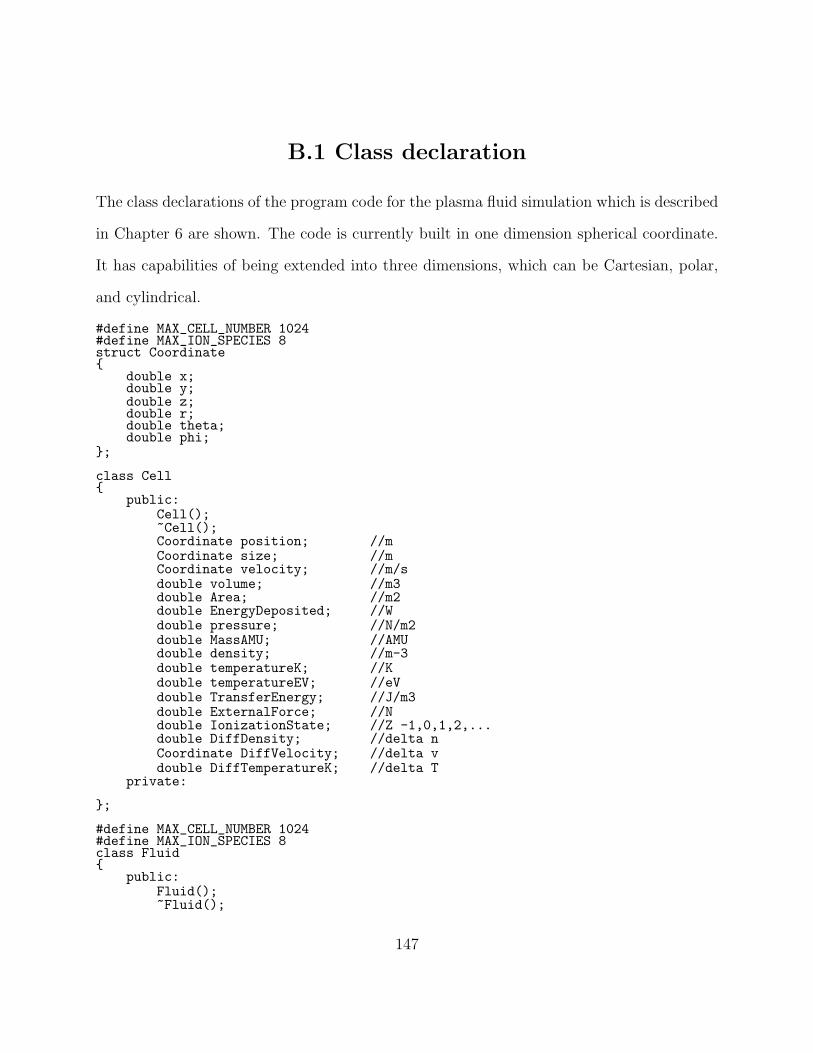
B.1 Class declaration
The class declarations of the program code for the plasma fluid simulation which is described
in Chapter 6 are shown. The code is currently built in one dimension spherical coordinate.
It has capabilities of being extended into three dimensions, which can be Cartesian, polar,
and cylindrical.
#define MAX_CELL_NUMBER 1024#define MAX_ION_SPECIES 8struct Coordinate
double x;double y;double z;double r;double theta;double phi;
;
class Cell
public:Cell();~Cell();Coordinate position; //mCoordinate size; //mCoordinate velocity; //m/sdouble volume; //m3double Area; //m2double EnergyDeposited; //Wdouble pressure; //N/m2double MassAMU; //AMUdouble density; //m-3double temperatureK; //Kdouble temperatureEV; //eVdouble TransferEnergy; //J/m3double ExternalForce; //Ndouble IonizationState; //Z -1,0,1,2,...double DiffDensity; //delta nCoordinate DiffVelocity; //delta vdouble DiffTemperatureK; //delta T
private:
;
#define MAX_CELL_NUMBER 1024#define MAX_ION_SPECIES 8class Fluid
public:Fluid();~Fluid();
147

int nMaxCell;int nMaxIons;int CellOrderElectrons[MAX_CELL_NUMBER];int CellOrderIons[MAX_ION_SPECIES][MAX_CELL_NUMBER];Cell Electrons[MAX_CELL_NUMBER];Cell Ions[MAX_ION_SPECIES][MAX_CELL_NUMBER];double ElectricField[MAX_CELL_NUMBER]; //V/mbool Process1DS(double DeltaT, double TimeStamp); //1 dimension sphericalvoid SummarizeCell1D();void ExportParameters(double TimeStamp);double AmbientPressure;double AmbientTemperatureK;
private:;
148

B.2 1D Process routine (method)
The class ”Fluid” has the following method that processes dynamics of the fluid with a given
time step. The method is specialized for a spherical coordinate and includes calculations of
divergence of the velocities. However it has no advanced conditional functions that check
negative density, temperature, cell size and so on.
bool Fluid::Process1DS(double DeltaT, double TimeStamp)
bool RetValue=true;
double SolidAngle=4*M_PI;double CoulombLogarism=10;double NuEI_1=4.0*sqrt(2.0/MassElectron*M_PI)*pow(eChargeUnit,4)*CoulombLogarism/3.0;//For first part friction coefficientdouble Alpha_1=4.0*sqrt(2.0*M_PI)*pow(eChargeUnit,4)*CoulombLogarism/3.0;//Processfor(int idx=1; idx<nMaxCell; idx++)
//ElectronsElectrons[idx].TransferEnergy=0;for(int idxIon=1; idxIon<nMaxIons; idxIon++)
double NuEI=NuEI_1*Electrons[idx].density*Ions[idxIon][idx].density*pow(Ions[idxIon][idx].IonizationState,2)/(kBoltzmann*Electrons[idx].temperatureK
*sqrt(kBoltzmann*Electrons[idx].temperatureK));Electrons[idx].TransferEnergy-=3.0/2.0*kBoltzmann*NuEI
*(Electrons[idx].temperatureK-Ions[idxIon][idx].temperatureK);double GradP=(Electrons[idx+1].pressure-Electrons[idx-1].pressure)
/Electrons[idx].size.r;//Electric FieldElectricField[idx]=-GradP/(Electrons[idx].density*eChargeUnit);//Energy balancedouble DivV=1/pow(Electrons[idx].position.r,2)
*(pow(Electrons[idx].position.r,2)*Electrons[idx].velocity.r-pow(Electrons[idx-1].position.r,2)*Electrons[idx-1].velocity.r)
/Electrons[idx].size.r;Electrons[idx].DiffDensity=-Electrons[idx].density*DivV*DeltaT;
//Momentum transferElectrons[idx].DiffTemperatureK=
2.0*DeltaT/(3.0*Electrons[idx].density*kBoltzmann)*(-Electrons[idx].pressure*DivV+Electrons[idx].TransferEnergy+Electrons[idx].EnergyDeposited/DeltaT);
//Ionsfor(int idxIon=0; idxIon<nMaxIons; idxIon++)
double NuEI=NuEI_1*Electrons[idx].density*Ions[idxIon][idx].density*pow(Ions[idxIon][idx].IonizationState,2)
/(kBoltzmann*Electrons[idx].temperatureK*sqrt(kBoltzmann*Electrons[idx].temperatureK));
Ions[idxIon][idx].TransferEnergy=3.0/2.0*kBoltzmann*NuEI*(Electrons[idx].temperatureK-Ions[idxIon][idx].temperatureK);
//Particle number conservationdouble DivV=1/pow(Ions[idxIon][idx].position.r,2)
*(pow(Ions[idxIon][idx].position.r,2)*Ions[idxIon][idx].velocity.r-pow(Ions[idxIon][idx-1].position.r,2)*Ions[idxIon][idx-1].velocity.r)
149

/Ions[idxIon][idx].size.r;Ions[idxIon][idx].DiffDensity=-Ions[idxIon][idx].density*DivV*DeltaT;//Momentum transferGradP=(Ions[idxIon][idx+1].pressure-Ions[idxIon][idx-1].pressure)
/Ions[idxIon][idx].size.r;//Friction force
double MassReduced;double Alpha=0;for(int idxIon2=0; idxIon2<nMaxIons; idxIon2++)
MassReduced=Ions[idxIon][idx].MassAMU*Ions[idxIon2][idx].MassAMU/(Ions[idxIon][idx].MassAMU+Ions[idxIon2][idx].MassAMU)*MassProton;
Alpha+=Alpha_1/sqrt(MassReduced)*pow(Ions[idxIon][idx].density*Ions[idxIon][idx].IonizationState,2)*MassReduced*(Ions[idxIon2][idx].velocity.r-Ions[idxIon][idx].velocity.r);
Ions[idxIon][idx].DiffVelocity.r=
DeltaT/(Ions[idxIon][idx].density*Ions[idxIon][idx].MassAMU*MassProton)*(-GradP-Alpha+Ions[idxIon][idx].ExternalForce);
//Energy balanceIons[idxIon][idx].DiffTemperatureK=
2.0*DeltaT/(3.0*Ions[idxIon][idx].density*kBoltzmann)*(-Ions[idxIon][idx].pressure*DivV+Ions[idxIon][idx].TransferEnergy);
//Post process//Process Time derivativesfor(int idx=1; idx<nMaxCell; idx++)
Electrons[idx].temperatureK+=Electrons[idx].DiffTemperatureK;if(Electrons[idx].temperatureK<0)
cout << "negative electron temperature at "<<idx<<endl;Electrons[idx].temperatureK=1e-30;RetValue=false;
Electrons[idx].temperatureEV=Electrons[idx].temperatureK/KperEV;for(int idxIon=0; idxIon<nMaxIons; idxIon++)
Ions[idxIon][idx].temperatureK+=Ions[idxIon][idx].DiffTemperatureK;if(Ions[idxIon][idx].temperatureK<0)
cout << "negative ion temperature at "<<idx<<endl;Ions[idxIon][idx].temperatureK=1e-30;RetValue=false;
Ions[idxIon][idx].temperatureEV=Ions[idxIon][idx].temperatureK/KperEV;Ions[idxIon][idx].density+=Ions[idxIon][idx].DiffDensity;if(Ions[idxIon][idx].density<0)
cout << "negative ion density at "<<idx<<endl;Ions[idxIon][idx].density=1e-30;RetValue=false;
Ions[idxIon][idx].velocity.r+=Ions[idxIon][idx].DiffVelocity.r;
//Calculate ve, nefor(int idx=1; idx<nMaxCell; idx++)
Electrons[idx].density=0;Electrons[idx].velocity.r=0;for(int idxIon=0; idxIon<nMaxIons; idxIon++)
double Zn=Ions[idxIon][idx].IonizationState*Ions[idxIon][idx].density;Electrons[idx].density+=Zn;Electrons[idx].velocity.r+=Zn*Ions[idxIon][idx].velocity.r;
Electrons[idx].velocity.r=Electrons[idx].velocity.r/Electrons[idx].density;
150

//Calculate motionfor(int idx=1; idx<nMaxCell; idx++)
Electrons[idx].position.r+=Electrons[idx].velocity.r*DeltaT;for(int idxIon=0; idxIon<nMaxIons; idxIon++)
Ions[idxIon][idx].position.r+=Ions[idxIon][idx].velocity.r*DeltaT;
//Calculate cell size, area, volume, pressurefor(int idx=1; idx<nMaxCell; idx++)
Electrons[idx].size.r=Electrons[idx].position.r-Electrons[idx-1].position.r;if(Electrons[idx].size.r<0)
RetValue=false;cout << "negative cell size at "<<idx<<endl;
Electrons[idx].Area=SolidAngle*pow(Electrons[idx].position.r,2);Electrons[idx].volume=Electrons[idx].size.r*Electrons[idx].Area;for(int idxIon=0; idxIon<nMaxIons; idxIon++)
Ions[idxIon][idx].size.r=Ions[idxIon][idx].position.r-Ions[idxIon][idx-1].position.r;if(Ions[idxIon][idx].size.r<0)
RetValue=false;cout << "negative cell size at "<<idx<<endl;
Ions[idxIon][idx].Area=SolidAngle*pow(Ions[idxIon][idx].position.r,2);Ions[idxIon][idx].volume=Ions[idxIon][idx].size.r*Ions[idxIon][idx].Area;Ions[idxIon][idx].pressure=Ions[idxIon][idx].density*kBoltzmann*Ions[idxIon][idx].temperatureK;
Electrons[idx].density=0;for(int idxIon=0; idxIon<nMaxIons; idxIon++)
Electrons[idx].density+=Ions[idxIon][idx].IonizationState*Ions[idxIon][idx].density;Electrons[idx].pressure=Electrons[idx].density*kBoltzmann*Electrons[idx].temperatureK;
if(RetValue==false)
ExportParameters(TimeStamp);return RetValue;
151

REFERENCES
[1] Attwood, D. T., Soft x-ray and extreme ultraviolet radiation: principle and applica-
tions, Cambridge University Press, 2000.
[2] Hoffnagle, J. A., Hinsberg, W. D., Sanchez, M., and Houle, F. A., ”Liquid immersion
deep-ultraviolet interferometric lithography,” J. Vac. Sci. and Tech. B, 17. pp. 3306-
3309, 1999.
[3] Liu, H-Y, Karklin, L., Wang, Y-T, and Pati, Y. C., ”Application of alternating
phase-shifting masks to 140-nm gate patterning: II.” Mask design and manufacturing
tolerances, proceedings of SPIE 3334, pp.2-14, 1998.
[4] Ronse, K., Beeck, M. Op de, Van den hove, L., and Engelen, J., ”Fundamental princi-
ples of phase shifting masks by Fourier optics: Theory and experimental verification,”
J. Vac. Sci. and Tech. B, 12, pp. 589-600, 1994.
[5] Mentor graphics, ”Lithography: The Integration of TCAD and EDA,”from
http://www.mentor.com/products/ic nanometer design/news/lithography tcad eda.cfm.
[6] Gwyn, C. W., Stulen, R., Sweeney, D., and Attwood, D., ”Extreme ultraviolet lithog-
raphy,” J. Vac. Sci. Tech. B 16, pp. 3142-3149, 1998.
[7] Sematech, proceedings are available at http://www.sematech.org.
[8] Tech News on ZDNet, Intel shows test chips made on future processes, Jan 25, 2006,
from http://news.zdnet.com/2100-9584 22-6030489.html.
152
[9] Kuerz, P. et. al., presentation at 4th EUVL symposium 2005, Nov. 2005, proceedings
are available at http://www.sematech.org.
[10] Moreau, W. M., Semiconductor Lithography, Plenum Publishing Co., New York, 1988.
[11] Slaughter J. M. et al., ”Structure and performance of Si/Mo multilayer mirrors for
the extreme ultraviolet,” J. Appl. Phys. 76, pp. 2144, 1994
[12] Watanabe, Y., ”Joint requirement,” Presentation at EUV Source workshop, Feb. 27
2005, proceedings available at www.sematech.org.
[13] Murakami, K., Presentation at EUV Source workshop, Oct. 29 2001, proceedings
available at www.sematech.org.
[14] Koay, C-S, George, S., Takenoshita, K., Bernath, R., Fujiwara, E., Richardson, M.,
and Bakshi, V., ”High conversion efficiency microscopic tin-doped droplet target laser-
plasma source for EUVL,” proceedings of SPIE 5751, pp. 279-292, 2005.
[15] Watanabe, Y., ”Joint requirement,” Presentation at EUV Source workshop, Feb. 22
2004, proceedings available at www.sematech.org.
[16] Paul Scherrer Institut, from http://sls.web.psi.ch/view.php/about/whatis/description/
whatis/index.html.
[17] Pankert, J. et. al., ”Physical Properties of the HCT EUV Source,” Proceedings of
SPIE 4688, pp. 87-93, 2002.
[18] Partlo, W., Fomenkov, I., Oliver, R., and Birx, D., ”Development of an EUV (13.5nm)
Light Source Employing a Dense Plasma Focus in Lithium Vapor,” Proceedings of
SPIE 3997, pp. 136-156, 2000.
153

[19] Schriever, G. et. al., ”Extreme ultraviolet light generation based on laser produced
plasmas (LPP) and gas discharge based pinch plasmas: A comparison of different
concepts,” proceedings of SPIE 3997, pp. 162-168, 2000.
[20] Klosner, M. A., Bender, H. A., Silfvast, W. T., and Rocca, J. J., ”Intense plasma
discharge source at 13.5 nm for extreme-ultraviolet lithography,” Opt. lett. 22, pp.
34-36 , 1997.
[21] Fomemkov, I. et. al., ”Characterization of a Dense Plasma Focus Device as a Light
Source for EUV Lithography,” presentation at 1st international symposium on EUVL,
Oct. 15, 2002, Dallas TX, proceeding is available at www.sematech.org.
[22] McNaught, S., ”Laser-Produced Plasma EUV Source Program, presentation at
EUVL source workshop,” Feb, 23, Santa Clara, CA, 2003, proceeding is available
at www.semetach.org.
[23] Center for x-ray optics, The Atomic Scattering Factor Files, available at www-
cxro.lbl.gov/optical constants/asf.html.
[24] Fraunhofer IOF, Image is found at www.iof.fraunhofer.de/departments/optical-
coatings/ media/mosi engl.pdf.
[25] Center for x-ray optics, X-ray tools, X-Ray Interactions With Matter, calculation
program is available at www-cxro.lbl.gov/optical constants/
[26] Yan, P., Zhang, G., Kofron, P., Chow, J., Stivers, A. R., Tejnil, E., Cardinale, G. F.,
and Kearney, P. A., ”EUV mask patterning approaches,” Proceedings of SPIE 3676,
pp. 309-313, 1999.
154

[27] Uzawa, S., ”Canon’s Development Status of EUVL Technologies,” presentation at
4th EUVL symposium, Nov. 7 2005, proceedings available at www.sematech.org.
[28] Jin, F., Gabel, K., Richardson, M. C., Kado, M., Vasil’Ev, A. F., Salzmann and
D., ”Mass-limited laserplasma cryogenic target for 13 nm point x ray sources for
lithography,” proceedings of. SPIE 2015, pp. 151-159, 1993.
[29] Dawson, J. M., ”In the Production of Plasma by Giant Pluse Lasers,” Phys. fluid
7, pp. 981-987, 1964; Johnston T. W. and Dawson, J. M., ”Correct values for high-
frequency power absorption by inverse bremsstrahlung in plasmas,” Phys. fluid 16,
pp. 722, 1973.
[30] Spitzer, L. Jr, Physics of Fully ionized gases, 2nd ed., Interscience publishers, New
York, 1962.
[31] George, S., Koay, C-S, Takenoshita, K., Bernath, R., Al-Rabban, M., Keyser, C.,
Bakshi, V., Scott, H. and Richardson, M., ”EUV spectroscopy of mass-limited Sn-
doped laser micro plasmas,” proceedings of SPIE 5751, pp. 779-788, 2005.
[32] O’onnel, D., ”Characterization of a Lithium laser produced plasma at 135 for extreme
ultraviolet projection lithography,” Master’s thesis, University of Central Florida,
1994.
[33] Saha, M. N., ”On a Physical Theory of Stellar Spectra,” Proc. of
Royal Society of London A, Containing Papars of a Mathematical and
Physical Character 99, pp. 135-153, 1921; Wolfram Research, from
http://scienceworld.wolfram.com/physics/SahaEquation.html.
155

[34] Kolb, A. C. and P. McWhirter, R. W. ”Ionization Rates and Power Loss from q-pinch
by Impurity Radiation,” Phys. Fluid 7, pp. 519-531, 1964.
[35] Peacook, N. J. and Pease, R. S., ”Source of highly stripped ions,” Brit. J. Appl. Phys.
(J. Phys. D), SER 2, Vol. 2, pp. 1705-1717, 1969.
[36] Colombant, D., and Tonon, D. F., ”X-ray emission in laser-produced plasmas,” J.
Appl. Phys. 44, pp.3524-3537, 1973.
[37] O’Sullivan, G. and Dunne, P., ”Spectroscopy of a 13.5 nm Laser Plasma Source,”
Presentation at Sematech EUVL Souce Workshop, Oct. 2002, proceedings available
at www.sematech.org
[38] Allen, C. W., Astrophysical Quantities, Athlone press, London, 1973.
[39] Tolstikhina, I. Yu., Churilov, S. S., Ryabtsev, A. N. and Koshelev, K. N., ”Atomic
Tin Data,” pp. 113-148, EUV Sources for lithography, Ed. Bakshi, V., SPIE press,
Washington, 2005.
[40] Braginskii, S. I., ”TRANSPORT PROCESS IN A PLASMA,” pp. 205-311, Review
of plasma physics, Consultants Bureau Enterprises, New York, 1965
[41] Mulser, P., ”ELECTROSTATIC FIELDS AND ION SEPERATION IN EXPAND-
ING LASER PRODUCED PLASMAS,” Plasma physics 13, pp. 1007-1012, 1971.
[42] Nagel, D. J., Brown, C. M., Peckerar, M. C., Ginter, M. L., Robinson, J. A., McIlrath,
T. J., Carroll, P. K., ”Repetitively pulsed-plasma soft x-ray source,” App. Opt. 23,
pp. 1428- 1433, 1984.
156

[43] Bridges, J. M., Cromer, C. L. and Mcilrath, T. J., ”Investigation of a laser-produced
plasma VUV light source.” Applied Optics 25, pp. 2208-2214, 1986.
[44] Helsinki University of Technology , advanced energy system, ”Pulsed Laser Deopsi-
tion,” from http://www.tkk.fi/Units/AES/projects/prlaser/pld.htm.
[45] Richardson, M., Silfvast, W., Bender, H. A., Hanzo, A., Yanovsky, V. P., Jin, F.
and Thorpe, J., ”Characterization and control of laser plasma flux parameters for
soft-x-ray projection lithography,” App. Phys. 32, pp. 6901-6910, 1993.
[46] Bender, H A., O’Connell, D. and Silfvast, W. T., ”Velocity characterization of partic-
ulate debris from laser-produced plasmas used for extreme-ultraviolet lithography,”
Appl. Opt. 34, pp. 6513-6521, 1995.
[47] Al-Rabban, M., 4th EUVL Symposium, Nov. 9 2005, proceedings available at
www.sematech.org.
[48] Rymell L. and Hertz, H. M., ”Droplet target for low-debris laser-plasma soft X-ray
generation,” Optics Communications 103 pp. 105-110, 1993.
[49] Kubiak, G. D., Bernardez II, L. J. and Krenz, K. D., ”High-power extreme-ultraviolet
source based on gas jets,” proceedings of SPIE 3331, pp. 81-89, 1998.
[50] Hansson, B. A. M., Rymell, L., Berglund M. and Hertz, H. M., ”Liquid-Xenon-Jet
Laser-Plasma X-Ray and EUV Source,” Microelectronic Engineering 53 pp. 667-670,
2000.
[51] Soumagne, G., Abe, T., Suganuma, T., Imai, Y., Someya, H., Hoshino, H., Nakano,
M., Komori, H., Takabayashi, Y., Ariga, T., Ueno, Y., Wada, Y., Endo, A. and Toy-
157

oda, K., ”Laser-Produced-Plasma Light Source for EUV Lithography,” Proceedings
of SPIE 5751, pp. 822-828, 2005.
[52] Jansson, P. A. C., Hansson, B. A. M., Hemberg, O., Otendal, M., Holmberg, A., de
Groot, J. and Hertz, H. M., ”Liquid-tin-jet laser-plasma extreme ultraviolet genera-
tion,” Appl. Phys. Lett. 84, pp. 2256-2258, 2004.
[53] Algots, J. M., Hemberg, O. and Bykanov, A., ”Liquid Metal Micro-Droplet Generator
for Laser Produced Plasma Target Delivery used in an Extreme Ultra-Violet Source,”
Proceedings of SPIE 5751, pp. 885-891, 2005.
[54] Richardson, M., Koay, C-S., Takenoshita, K., Keyser, C., George, S., Teerawattan-
sook, S., Al-Rabban, M. and Scott, H., ”Laser plasma EUVL sources progress and
challenges,” Proceedings of SPIE 5751, pp. 447-453, 2005.
[55] Pankert, J., Bergmann, K., Klein, J., Neff, W., Rosier, O., Seiwert, S., Smith, C.,
Probst, S., Vaudrevange, D., Siemons, G., Apetz, R., Jonkers, J., Loeken, M., Derra,
G., Kruecken, T. and Zink, P., ”Status of Philips’ extreme UV source,” Proceedings
of SPIE 5751, pp. 152-159, 2005.
[56] Partlo, IW. N., Fomenkov, I. V. and Birx, D. L., ”EUV (13.5-nm) light generation
using a dense plasma focus device,” Proceedings of SPIE 3676, pp. 846-858, 1999.
[57] Richardson, M., US Patent 6865,255, Mar, 2005.
[58] Keyser, C., ”Optical and spectral characterization of the water droplet laser plasma
EUV source,” Ph. D. thesis, University of Central Florida, 2003.
158

[59] Koay, C-S, ”Radiation studies of the tin-doped microscopic drolet laser plasma light
source specific to EUV lithography,” Ph. D. thesis University of Central Florida, 2006.
[60] Fujioka, S. et. al., ”Properties of EUV and particle generations from laser-irradiated
solid- and low-density tin targets,” proceedings of SPIE 5751, pp. 578-587, 2005.
[61] Tomie, T., Aota, T., Quan Lin, J., Ueno, Y., Yashiro, H., Kandaka, N., Moriwaki,
H., Niimi, G., Matsushima, I. and Nishigori, K., ”Particle-cluster tin target for a high
conversion efficiency LPP source for EUVL,” proceedings of SPIE 5374, pp. 383-393,
2004.
[62] Dusterer, S., Schwoerer, H., Ziegler, W., Salzmann, D. and Sauerbrey, R., ”Effects
of a prepulse on laser-induced EUV radiation conversion efficiency,” Appl. Phys. 76,
pp. 17-21, 2003.
[63] Rayleigh, L., Proceedings of the London mathematical society, 10, pp. 4-13, 1879;
Lindblad, N. R. and Schneider, J. M. ”Production of uniform-sized liquid droplets,”
J. Sci. instrum. 42, pp. 632-638, 1965.
[64] Kaminsky, M., Atomic and ionic impact phenomena on matal surfaces, Academic
press, New York, 1965.
[65] Xu, S., Tay, B. K., Tan, H. S., Zhong, L., Tu, Y. Q., Silva, S. R. P. and Milne, W. I.,
”Properties of carbon ion deposited tetrahedral amorphous carbon films as a function
of ion energy,” J. Appl. Phys 79, pp 7234- 7240, 1996.
[66] Matsunari, S., Aoki, T., Gomei, Y., Terashima, S., Takase, H., Niibe, M., Kakutani,
Y., ”Lifetime estimation and improvement of capping layer on multilayer mirror for
159
EUV lithography in EUVA,” presentation at 4th EUVL symposium Nov. 8, 2005,
proceedings available at www.sematech.org.
[67] Heun, S., Kremmer, S., Ercolani, D., Wurmbauer, H. and Teichert, C., ”Behavior of
SiO2 nanostructures under intense extreme ultraviolet illumination,” J. Appl. Phys.
97, pp. 104333 (4pages), 2005.
[68] Klebanoff, L. E., Malinowski, M. E., Grunow, P. A., Clift, W. M., Steinhaus, C.,
Leung, A. H. and Haney, S. J., ”First environmental data from the EUV engineering
test stand,” Proceedings of SPIE 4343, pp. 342-346, 2001.
[69] Nishiyama, I., Oizumi, H., Motai, K., Izumi, A., Ueno, T., Akiyama, H. and Namiki,
A., ”Reduction of oxide layer on Ru surface by atomic-hydrogen treatment,” J. Vac.
Sci.Tech. B, 23, pp. 3129-3131, 2005.
[70] Tichenor D. A. et. al, ”EUV engineering test stand,” Proceedings of SPIE 3997, pp.
48-69, 2000.
[71] Hill, S. B., Tarrio, C., Lucatorto, T. B., Madey, T. E., Bajt, S., Wood II, O., Wurm,
S. and Edwards, N. V., ”EUV Endurance Testing of Ruthenium-Capped Multilayer
Mirrors,” presentation at 4th EUVL symposium, Nov. 8 2005, proceedings available
at www.sematech.org.
[72] Klebanoff, L. E., Malinowski, M. E., Clift, W. M., Steinhaus, C. and Grunow, P.,
”Use of gas-phase ethanol to mitigate extreme UV/water oxidation of extreme UV
optics,” J. Vac. Sci. Tech. A, 22, pp. 425-432, 2004.
160

[73] Nishiyama, I., ”Model of Ru surface oxidation for the lifetime scaling of EUVL pro-
jection optics mirror,” presentation at 4th EUVL Sympsium Nov. 8 2005, proceedings
available at www.sematech.org.
[74] Grunow, P. A., Klebanoff, L. E., Graham, Jr. S., Haney, S. J., Clift, W. M., ”Rates
and Mechanisms of Optic Contamination in the EUV Engineering Test Stand,” pro-
ceedings of SPIE 5037, pp. 418-428, 2003.
[75] Anderson, R. J., Buchenauer, D. A., Klebanoff, L., Wood II, O. R. and Edwards,
N. V., ”The erosion of materials exposed to a laser-pulsed plasma (LPP) extreme
ultraviolet (EUV) illumination source,” proceedings of SPIE 5374, pp. 710-719, 2004.
[76] Schriever, G., Richardson, M. C. and Turcu, E., ”The droplet laser plasma source for
EUV lithography,” Proceedings of CLEO, pp. 393-394, 2000.
[77] Ziegler, J. F., ”SRIM-2003,” Nucl. Instr. Meth. Phys. Res. B 219-220, pp. 1027-1036,
2004.
[78] Ziegler, J. F., SRIM-2003, software available at www.srim.org.
[79] Tian, S., ”Predictive Monte Carlo ion implantation simulator from sub-keV to above
10 MeV,” J Appl. Phys. 93, pp. 5893-5904, 2003.
[80] Ecke, G., Kosiba, R., Kharlamov, V., Trushin, Y. and Pezoldt, J., ”The estimation
of sputtering yields for SiC and Si,” Nuclear Inst. & Physics Research B. 196, pp.
39-50, 2002.
161
[81] Miyake, A., Amemiya, M., Masaki, F. and Watanabe, Y., ”Phase measurement of
reflection of EUV multilayer mirror using EUV standing waves,” J. Vac. Sci. Tech. B
22, pp 2970-2974, 2004.
[82] QCM research, ”Mass conversion example,” at http://qcmresearch.com/mass.htm.
[83] Whilte, R. M., ”SURFACE ACOUSTIC WAVE SENSORS,”pproceedings of Ultra-
sonics Symposium IEEE 1985, 490-494, 1985.
[84] Particle measuring systems, inc. Exhibition at SPIE microlithography 2004, informa-
tion available at www.pmeasuring.com/aux/home.
[85] Online article on sensors, article found at www.sensormag.com/articles/1000/68/
main.shtml.
[86] Hansson, B. A. M., Hemberg, O., Hertz, H. M., Berglund, M., Choi, H.-J., Jacobsson,
B., Janin, E., Mosesson, S., Rymell, L., Thoresen, J. and Wilner, M., ”Characteri-
zation of a liquid-xenon-jet laser-plasma extreme-ultraviolet source,” Rev. Sci. Instr.
75, pp. 2122-2129, 2004.
[87] Komori, H., Imai, Y., Soumagne, G., Abe, T., Suganuma, T. and Endo, A., ”Magnetic
field ion mitigation for EUV light sources,” Proceedings of SPIE 5751, pp. 859-866,
2005.
[88] Gerdin, G., Stygar, W. and Venneri, F., ”Faraday cup analysis of ion beams produced
by a dense plasma focus,” J. App. Phys. 52, pp. 3269-3275, 1981.
162

[89] Bilek, M. M. M., Chhowalla, M., Weiler, M. and Milne, W. I., ”Ion energy and
plasma characterization in a silicon filtered cathodic vacuum arc,” J. App. Phys. 79,
pp. 1287-1291, 1996.
[90] Nassisi V. and Pedone, A., ”Physics of the expanding plasma ejected from a small
spot illumined by an ultraviolet pulsed laser,” Rev. Sci. Instr. 74, pp. 68-72, 2003.
[91] Takenoshita, K., Koay, C-S, Richardson, M. C. and Turcu, I. C. E., ”Repeller field
debris mitigation approach for EUV sources,” proceedings of SPIE 5037, pp. 792-800,
2003.
[92] Takenoshita, K., Koay, C-S, Teerawattansook, S., Richardson, M. and Bakshi, V.,
”Debris characterization and mitigation from microscopic laser-plasma tin-doped
droplet EUV sources,” proceedings of SPIE 5751, pp. 563-571, 2005.
[93] BURLE INDUSTRIES, INC., ”Channeltron-electron multiplier hand-
book for mass spectrometry applications,” from http://www.burle.com/cgi-
bin/byteserver.pl/pdf/ChannelBook.pdf.
[94] Christiansen, J. P., Ashby, D. E. T. F. and Roberts, K. V., ”MEDUSA A one-
dimensional Laser fusion code,” Computer Physics Communications, 7, pp271-287,
1974.
[95] Ginter M. L. and Mcilrath, T. J., ”Debris and VUV emission from a laser-produced
plasma operated at 150 Hz using a krypton fluoride laser,” Appl. Opt. 27, pp. 885-889,
1988.
[96] Rymell L. and Hertz, H. M., ”Debris eliminatio in a droplet-target Baser-plasma soft
x-ray source,” Rev. Sci. Instrum. 66, pp. 4916-4920, 1995.
163

[97] Jurczyk, B. E., Lopez, E. V., Neumann, M. J. and Ruzic, D. N., ”Illinois Debris-
Mitigation EUV Applications Laboratory (IDEAL),” Proceedings of SPIE 5374, pp.
695-701, 2004.
[98] Yashiro, H., Aota, T., Nishigori, K., Ueno, Y. and Tomie, T., ”Ultra fast ion shutter
employing a laser-produced plasma,” Proceedings of SPIE, 5037, pp. 759-766, 2003.
[99] Shmaenok, L. A., de Bruijn, C. C., Fledderus, H. F., Stuik, R., Schmidt, A. A.,
Simanovski, D. M., Sorokin, A. V., Andreeva, T. A. and Bijkerk, F., ”Demonstration
of a foil trap technique to eliminate laser plasma atomic debris and small particulates,”
Proceedings of SPIE 3331, pp. 90-94, 1998.
[100] Komori, H., Soumagne, G., Hoshino, H., Abe, T., Suganuma, T., Imai, Y., Endo,
A. and Toyoda, K., ”Ion damage analysis on EUV collector mirrors,” Proceedings of
SPIE, 5374, pp. 839-846, 2004.
[101] Boeuf, J. P. and Punset, C., ”PHYSICS AND MODELLING OF DUSTY PLAS-
MAS,” pp 1-76, DUSTY PLASMAS, Physics, Chemistry and Technological Impacts
in Plasma Processing, Ed. Bouchoule, A., Jhon Wiley & Sons, Chichester, 1999.
[102] Paschen, F., Annalen der physic und Chemie 37, 69, 1889; Lisovskiy, V. A., Yakovin,
S. D. and Yegorenkov, V. D., ”Low-pressure gas breakdown in uniform dc electric
field,” J. Phys. D: Appl. Phys. 33, pp. 2722-2730, 2000.
164
Related Documents