Death to Kappa: birth of quantity disagreement and allocation disagreement for accuracy assessment

This article was downloaded by: [Clark University], [Robert Pontius]On: 17 August 2011, At: 07:27Publisher: Taylor & FrancisInforma Ltd Registered in England and Wales Registered Number: 1072954 Registeredoffice: Mortimer House, 37-41 Mortimer Street, London W1T 3JH, UK

International Journal of RemoteSensingPublication details, including instructions for authors andsubscription information:http://www.tandfonline.com/loi/tres20

Death to Kappa: birth of quantitydisagreement and allocationdisagreement for accuracy assessmentRobert Gilmore Pontius Jr a & Marco Millones aa School of Geography, Clark University, Worcester, MA, 01610,USA

Available online: 17 Aug 2011

To cite this article: Robert Gilmore Pontius Jr & Marco Millones (2011): Death to Kappa: birth ofquantity disagreement and allocation disagreement for accuracy assessment, International Journalof Remote Sensing, 32:15, 4407-4429

To link to this article: http://dx.doi.org/10.1080/01431161.2011.552923

PLEASE SCROLL DOWN FOR ARTICLE

Full terms and conditions of use: http://www.tandfonline.com/page/terms-and-conditions

This article may be used for research, teaching and private study purposes. Anysubstantial or systematic reproduction, re-distribution, re-selling, loan, sub-licensing,systematic supply or distribution in any form to anyone is expressly forbidden.

The publisher does not give any warranty express or implied or make any representationthat the contents will be complete or accurate or up to date. The accuracy of anyinstructions, formulae and drug doses should be independently verified with primarysources. The publisher shall not be liable for any loss, actions, claims, proceedings,demand or costs or damages whatsoever or howsoever caused arising directly orindirectly in connection with or arising out of the use of this material.

http://www.tandfonline.com/loi/tres20

http://dx.doi.org/10.1080/01431161.2011.552923

http://www.tandfonline.com/page/terms-and-conditions

http://www.tandfonline.com/page/terms-and-conditions

International Journal of Remote SensingVol. 32, No. 15, 10 August 2011, 4407–4429

Death to Kappa: birth of quantity disagreement and allocationdisagreement for accuracy assessment

ROBERT GILMORE PONTIUS JR* and MARCO MILLONESSchool of Geography, Clark University, Worcester, MA 01610, USA

(Received 27 August 2010; in final form 20 December 2010) 5

The family of Kappa indices of agreement claim to compare a map’s observedclassification accuracy relative to the expected accuracy of baseline maps that canhave two types of randomness: (1) random distribution of the quantity of each cat-egory and (2) random spatial allocation of the categories. Use of the Kappa indiceshas become part of the culture in remote sensing and other fields. This article exam- 10

ines five different Kappa indices, some of which were derived by the first author in2000. We expose the indices’ properties mathematically and illustrate their limi-tations graphically, with emphasis on Kappa’s use of randomness as a baseline,and the often-ignored conversion from an observed sample matrix to the estimatedpopulation matrix. This article concludes that these Kappa indices are useless, mis- 15

leading and/or flawed for the practical applications in remote sensing that we haveseen. After more than a decade of working with these indices, we recommend thatthe profession abandon the use of Kappa indices for purposes of accuracy assess-ment and map comparison, and instead summarize the cross-tabulation matrixwith two much simpler summary parameters: quantity disagreement and alloca- 20

tion disagreement. This article shows how to compute these two parameters usingexamples taken from peer-reviewed literature.

1. Introduction

The proportion of observations classified correctly is perhaps the most commonlyused measurement to compare two different expressions of a set of categories, for 25

example, to compare land-cover categories expressed in a map and to reference datacollected for the map’s accuracy assessment. There are good reasons for the popular-ity of the proportion correct measurement. Proportion correct is simple to compute,easy to understand and helpful to interpret. Nevertheless, it has become customaryin the remote-sensing literature to report the Kappa index of agreement along with 30

proportion correct, especially for purposes of accuracy assessment, since Kappa alsocompares two maps that show a set of categories. Kappa is usually attributed to Cohen(1960), but Kappa has been derived independently by others, and citations go backmany years (Galton 1892, Goodman and Kruskal 1954, Scott 1955). Kappa becamepopularized in the field of remote sensing and map comparison by Congalton (1981), 35

Congalton et al. (1983), Monserud and Leemans (1992), Congalton and Green (1999),Smits et al. (1999) and Wilkinson (2005), to name a few. In particular, Congalton and

*Corresponding author. Email: [email protected]

International Journal of Remote SensingISSN 0143-1161 print/ISSN 1366-5901 online © 2011 Taylor & Francis

http://www.tandf.co.uk/journalsDOI: 10.1080/01431161.2011.552923

Dow

nloa

ded

by [

Cla

rk U

nive

rsity

], [

Rob

ert P

ontiu

s] a

t 07:

27 1

7 A

ugus

t 201

1

4408 R. G. Pontius Jr. and M. Millones

Green (2009, p. 105) state that ‘Kappa analysis has become a standard component ofmost every accuracy assessment (Congalton et al. 1983, Rosenfield and Fitzaptrick-Linz 1986, Hudson and Ramm 1987, Congalton 1991) and is considered a required 40

component of most image analysis software packages that include accuracy assess-ment procedures’. Indeed, Kappa is published frequently and has been incorporatedinto many software packages (Visser and de Nijs 2006, Erdas Inc. 2008, Eastman2009).

The use of Kappa continues to be pervasive in spite of harsh criticisms for decades 45

from many authors (Brennan and Prediger 1981, Aickin 1990, Foody 1992, Ma andRedmond 1995, Stehman 1997, Stehman and Czaplewski 1998, Foody 2002, Turk2002, Jung 2003, Di Eugenio and Glass 2004, Foody 2004, Allouche et al. 2006, Foody2008). Congalton and Green (2009, p. 115) acknowledge some of these criticisms, butthey report that Kappa ‘must still be considered a vital accuracy assessment measure’. 50

If Kappa were to reveal information that is different from proportion correct in amanner that has implications concerning practical decisions about image classifica-tion, then it would be vital to report both proportion correct and Kappa; however,Kappa does not reveal such information. We do not know of any cases where the pro-portion correct was interpreted, and then the interpretation was changed due to the 55

calculation of Kappa. In the cases that we have seen, Kappa gives information that isredundant or misleading for practical decision making.

Pontius (2000) exposed some of the conceptual problems with the standard Kappadescribed above and proposed a suite of variations on Kappa in an attempt to remedythe flaws of the standard Kappa. After a decade of working with these variations, 60

we have found that they too possess many of the same flaws as the original standardKappa. The standard Kappa and its variants are frequently complicated to compute,difficult to understand and unhelpful to interpret. This article exposes problems withthe standard Kappa and its variations. It also recommends that our profession replacethese indices with a more useful and simpler approach that focuses on two components 65

of disagreement between maps in terms of the quantity and spatial allocation of thecategories. We hope this article marks the end of the use of Kappa and the beginning ofthe use of these two components: quantity disagreement and allocation disagreement.

2. Methods

2.1 Maps to show concepts 70

We illustrate our points by examining the maps in figure 1. Each map consists of ninepixels, and each pixel belongs to either the white category denoted by 0 or the blackcategory denoted by 1. The rectangle with the abbreviation ‘refer.’ in the bottom rowindicates the reference map, which we compare to all of the other maps, called thecomparison maps. The comparison maps are arranged from left to right in order of 75

the quantity of the black pixels they contain. We can think of this quantity as theamount of black ink used to print the map. We introduce this ink analogy because theanalogy is helpful to explain the concepts of quantity disagreement and allocation dis-agreement. All the maps within a single column contain an identical quantity of blackpixels, indicated by the number at the bottom of the column. Within a column, the 80

order of the maps from bottom to top matches the order of the amount of disagree-ment. Specifically, the maps in the bottom row show an optimal spatial allocation thatminimizes disagreement with the reference map, given the quantity of black pixels;while the maps at the top row of each column show a spatial allocation that maximizes

Dow

nloa

ded

by [

Cla

rk U

nive

rsity

], [

Rob

ert P

ontiu

s] a

t 07:

27 1

7 A

ugus

t 201

1

Death to Kappa 4409

Figure 1. Reference (refer.) map and comparison maps that show all possible combinationsof quantity disagreement and allocation disagreement. The dotted box highlights a comparisonmap that has three pixels of disagreement, where the two pixels of disagreement at the bottomare omission disagreement for the black category and the one pixel in the upper right is commis-sion disagreement for the black category. This implies that the comparison map in the dottedbox has one pixel of quantity disagreement and two pixels of allocation disagreement, since twopixels in the comparison map could be reallocated in a manner that would increase agreementwith the reference map.

disagreement with the reference map, given the quantity of black pixels, that is, given 85

the amount of black ink in the map. The concepts of quantity and allocation have beenexpressed by different names in other literature. In the field of landscape ecology, theword ‘composition’ describes the quantity of each category, and the word ‘configura-tion’ describes the allocation of the categories in terms of spatial pattern (Gergel andTurner 2002, Remmel 2009). In figure 1, each different column has a unique compo- 90

sition of black and white, while there are various configurations within each column.There are a few other possible configurations of black and white to construct the com-parison maps in addition to those shown in figure 1. However, we do not show thoseconfigurations because figure 1 gives a set of comparison maps that demonstrate allpossible combinations of quantity disagreement and allocation disagreement. 95

We define quantity disagreement as the amount of difference between the referencemap and a comparison map that is due to the less than perfect match in the propor-tions of the categories. For example, the reference map in figure 1 has three black pixelsand six white pixels. The three comparison maps above the reference map in figure 1have zero quantity disagreement with the reference map because they also have three 100

black pixels and six white pixels. Each comparison map in a different column than thereference map has positive quantity disagreement, which is equal to the absolute valueof the comparison map’s number of black pixels minus three. We can think of quantitydisagreement as the difference in the amount of black ink used to produce the refer-ence map versus the amount of black ink used to produce the comparison map. This 105

ink analogy extends to a multi-category case, where each category is a different colourof ink.

We define allocation disagreement as the amount of difference between the referencemap and a comparison map that is due to the less than optimal match in the spatialallocation of the categories, given the proportions of the categories in the reference and 110

comparison maps. Again, the ink analogy is helpful, since we can envision various

Dow

nloa

ded

by [

Cla

rk U

nive

rsity

], [

Rob

ert P

ontiu

s] a

t 07:

27 1

7 A

ugus

t 201

1


ways in which the ink can be allocated spatially within the comparison map, wheresome allocations have a better match with the reference map than other allocations.For example, each column of comparison maps in figure 1 is ordered from bottom totop in terms of increasing allocation disagreement. Allocation disagreement is always 115

an even number of pixels because allocation disagreement always occurs in pairs ofmisallocated pixels. Each pair consists of one pixel of omission for a particular cate-gory and one pixel of commission for the same category. A pixel is called omission forthe black category when the pixel is black in the reference map and not black in thecomparison map. A pixel is called commission for the black category when the pixel is 120

black in the comparison map and not black in the reference map. If a comparison maphas pixels of both omission and commission for a single category, then it is possible toenvision swapping the positions of the omitted and committed pixels within the com-parison map so that the rearranged allocation has a better match with the referencemap. If it is possible to perform such swapping, then there exists a positive amount 125

of allocation disagreement in the original comparison map (Alo and Pontius 2008).Previous literature calls this type of disagreement ‘location disagreement’, but we havefound that scientists frequently misinterpret this term by calling any disagreement ina map ‘location disagreement’. Therefore, we recommend that the profession beginusing the term ‘allocation disagreement’ instead of ‘location disagreement’, as this 130

article does. Figure 1 highlights a particular comparison map that this article uses toexplain the concepts in depth. This particular comparison map has one pixel of quan-tity disagreement and two pixels of allocation disagreement for a total disagreementof three pixels.

2.2 Disagreement space 135

Figure 2 plots the total disagreement versus the quantity of the black category forthe maps in figure 1. Circles denote the maps in the bottom row of figure 1 that havezero allocation disagreement, such that the total disagreement is attributable entirelyto the less than perfect match between the reference map and the comparison map interms of the quantity of black and white pixels. Quantity disagreement is the name 140

for this type of less than perfect match, and it is measured as the distance betweenthe horizontal axis and the diagonally oriented boundary of quantity disagreement.For all plotted points above the quantity disagreement boundary, the correspondingcomparison map contains a positive amount of allocation disagreement. The total dis-agreement is the sum of the quantity disagreement and the allocation disagreement. In 145

other words, the allocation disagreement is the total disagreement minus the quantitydisagreement, as shown in figure 2 for the comparison map highlighted in figure 1.Triangles in figure 2 denote the maps in the top of each column in figure 1, which havethe maximum possible allocation disagreement. It is mathematically impossible forany maps to fall outside the rectangle defined by the quantity disagreement and maxi- 150

mum disagreement boundaries. All of the diamonds denote maps that have two pixelsof allocation disagreement, and all of the squares denote maps that have four pixels ofallocation disagreement. The dashed line in figure 2 shows the statistical expectationof disagreement for a comparison map where the spatial allocation is random, giventhe quantity of black pixels. The central asterisk shows the statistical expectation of 155

disagreement for a comparison map where both quantity and allocation of the pixelsin the comparison map are random.

Dow

nloa

ded

by [

Cla

rk U

nive

rsity

], [

Rob

ert P

ontiu

s] a

t 07:

27 1

7 A

ugus

t 201

1

Death to Kappa 4411

9

8

7

6

5

4

Tota

l dis

ag

reem

ent (n

um

ber

of

pix

els

)

3

2

1

00 1 2 3 4

Quantity of black category in comparison map (number of pixels)

5 6 7 8 9

Allocation disagreement

Quantity disagreement

Maximum disagreement

Two pair misallocation

Random allocation

One pair misallocation


Figure 2. Disagreement space for all comparison maps, showing quantity disagreement andallocation disagreement for the highlighted comparison map in figure 1.

2.3 Mathematical notation for an unbiased matrix

A cross-tabulation matrix is the mathematical foundation of proportion correct andthe various Kappa indices. The cross-tabulation matrix has many other names, includ- 160

ing confusion matrix, error matrix and contingency table. It is essential that the matrixgives unbiased information concerning the entire study area in order to derive unbi-ased summary statistics. If reference data are available for all pixels, as is the casein figure 1, then the matrix gives unbiased information concerning the relationshipbetween the reference map and the comparison map; hence, the matrix is analysed 165

directly. However, reference information for an entire study area frequently does notexist in practice due to time limitations, financial constraints, inaccessibility or unavail-ability. In those cases, a sampling strategy is typically implemented to collect a sampleof reference data from the landscape (Stehman and Czaplewski 1998, Stehman 2009).This subsection gives the mathematical notation for the popular stratified sampling 170

design, where the strata are the categories in the comparison map. We present themathematics to convert the observed sample matrix into an estimated unbiased pop-ulation matrix because we have found that this crucial step is frequently ignored inpractice.

In our notation, the number of categories is J, so the number of strata is also J in 175

a typical stratified sampling design. Each category in the comparison map is denotedby an index i, which ranges from 1 to J. The number of pixels in each stratum is Ni.Random selection of the pixels within each stratum assures that the sample from eachstratum is representative of that stratum. Reference information is collected for eachobservation in the sample. Each observation is tallied based on its category i in the 180

comparison map and its category j in the reference information. The number of suchobservations is summed to form the entry nij in row i and column j of the samplematrix.

Dow

nloa

ded

by [

Cla

rk U

nive

rsity

], [

Rob

ert P

ontiu

s] a

t 07:

27 1

7 A

ugus

t 201

1


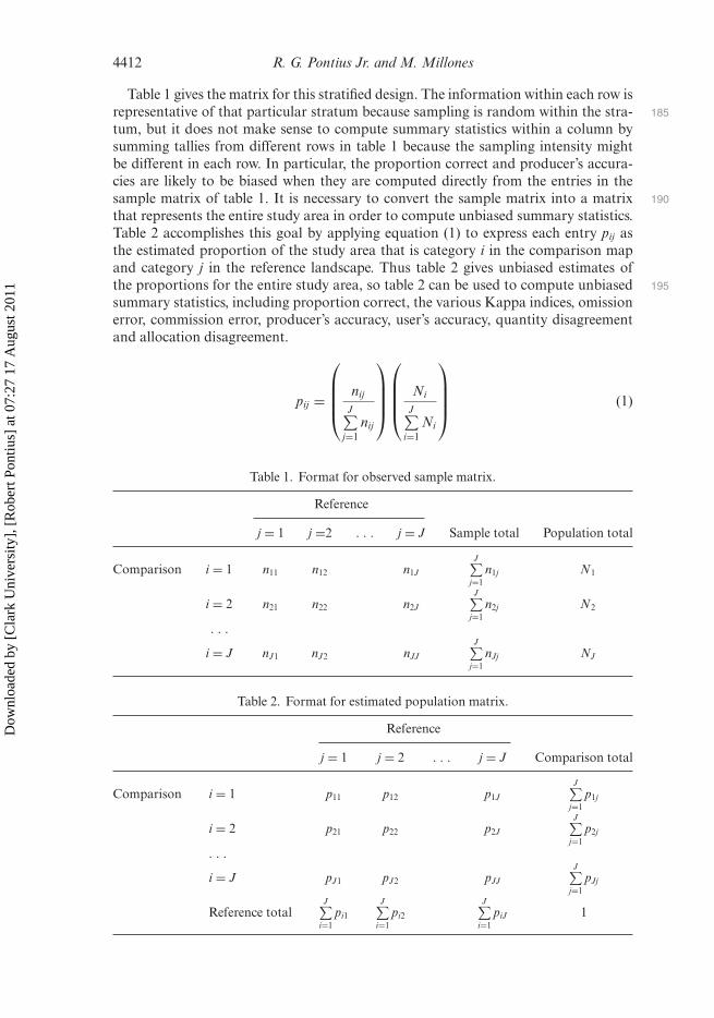
Table 1 gives the matrix for this stratified design. The information within each row isrepresentative of that particular stratum because sampling is random within the stra- 185

tum, but it does not make sense to compute summary statistics within a column bysumming tallies from different rows in table 1 because the sampling intensity mightbe different in each row. In particular, the proportion correct and producer’s accura-cies are likely to be biased when they are computed directly from the entries in thesample matrix of table 1. It is necessary to convert the sample matrix into a matrix 190

that represents the entire study area in order to compute unbiased summary statistics.Table 2 accomplishes this goal by applying equation (1) to express each entry pij asthe estimated proportion of the study area that is category i in the comparison mapand category j in the reference landscape. Thus table 2 gives unbiased estimates ofthe proportions for the entire study area, so table 2 can be used to compute unbiased 195

summary statistics, including proportion correct, the various Kappa indices, omissionerror, commission error, producer’s accuracy, user’s accuracy, quantity disagreementand allocation disagreement.

pij =

⎛⎜⎜⎜⎝ nij

J∑j=1

nij

⎞⎟⎟⎟⎠⎛⎜⎜⎜⎝ Ni

J∑i=1

Ni

⎞⎟⎟⎟⎠ (1)

Table 1. Format for observed sample matrix.

Reference

j = 1 j =2 . . . j = J Sample total Population total

Comparison i = 1 n11 n12 n1J

J∑j=1

n1j N1

i = 2 n21 n22 n2J

J∑j=1

n2j N2

. . .

i = J nJ1 nJ2 nJJ

J∑j=1

nJj NJ

Table 2. Format for estimated population matrix.

Reference

j = 1 j = 2 . . . j = J Comparison total

Comparison i = 1 p11 p12 p1J

J∑j=1

p1j

i = 2 p21 p22 p2J

J∑j=1

p2j

. . .

i = J pJ1 pJ2 pJJ

J∑j=1

pJj

Reference totalJ∑

i=1pi1

J∑i=1

pi2

J∑i=1

piJ 1

Dow

nloa

ded

by [

Cla

rk U

nive

rsity

], [

Rob

ert P

ontiu

s] a

t 07:

27 1

7 A

ugus

t 201

1

Death to Kappa 4413

2.4 Parameters to summarize the population matrix

There are numerous possible parameters to summarize the information in the 200

population matrix (Ma and Redmond 1995, Fielding and Bell 1997, Stehman 1997,Liu et al. 2007). This article focuses on the Kappa indices of agreement and twosimpler measures: quantity disagreement and allocation disagreement (Pontius 2000,2002, Pontius and Suedmeyer 2004, Pontius et al. 2007). All the calculations derivedirectly from the proportions in table 2. Equation (2) computes the quantity disagree- 205

ment qg for an arbitrary category g, since the first summation in equation (2) is theproportion of category g in the reference map and the second summation is the propor-tion of category g in the comparison map. Equation (3) computes the overall quantitydisagreement Q incorporating all J categories. Equation (3) must divide the summa-tion of the category-level quantity disagreements by two because an overestimation 210

in one category is always accompanied by an underestimation in another category,so the summation double counts the overall quantity disagreement. For the examplein figure 1, the overall quantity disagreement is equal to the quantity disagreementfor black plus the quantity disagreement for white, then divided by two. Equation (4)computes the allocation disagreement ag for an arbitrary category g, since the first 215

argument within the minimum function is the omission of category g and the sec-ond argument is the commission of category g. The multiplication by two and theminimum function are necessary in equation (4) because allocation disagreement forcategory g comes in pairs, where commission of g is paired with omission of g, so thepairing is limited by the smaller of commission and omission (Pontius et al. 2004). 220

Equation (5) gives the overall allocation disagreement A by summing the category-level allocation disagreements. Equation (5) divides the summation by two because thesummation double counts the overall allocation difference, just as the summation ofequation (3) double counts the overall quantity difference. Equation (6) computes theproportion correct C. Equation (7) shows how the total disagreement D is the sum of 225

the overall quantity disagreement and overall allocation disagreement. The appendixgives a mathematical proof of equation (7).

qg =∣∣∣∣∣∣(

J∑i=1

pig

)−⎛⎝ J∑

j=1

pgj

⎞⎠∣∣∣∣∣∣ (2)

Q =

J∑g=1

qg

2(3)

ag = 2 min

⎡⎣(

J∑i=1

pig

)− pgg,

⎛⎝ J∑

j=1

pgj

⎞⎠− pgg

⎤⎦ (4)

A =

J∑g=1

ag

2(5)

C =J∑

j=1

pjj (6)

Dow

nloa

ded

by [

Cla

rk U

nive

rsity

], [

Rob

ert P

ontiu

s] a

t 07:

27 1

7 A

ugus

t 201

1


D = 1 − C = Q + A (7)

Equations (8)–(10) begin to construct the calculations to compute the Kappaindices. Equation (8) gives the expected agreement eg for category g, assuming random 230

spatial allocation of category g in the comparison map, given the proportions of cate-gory g in the reference and comparison maps. Equation (9) gives the overall expectedagreement E assuming random spatial allocation of all categories in the comparisonmap, given the proportions of those categories in the reference and comparison maps.Equation (9) defines E for convenience because E is eventually used in the equations 235

for some of the Kappa indices. Equation (10) defines the overall expected disagreementR as equal to 1 – E, so we can express the Kappa indices as ratios of disagreement, asopposed to ratios of agreement, which will be helpful when we explain the figures inthe results section.

eg =(

J∑i=1

pig

)⎛⎝ J∑j=1

pgj

⎞⎠ (8)

E =J∑

g=1

eg (9)

R = 1 − E (10)

Equations (11)–(15) define five types of Kappa indices. Each Kappa is an index that 240

attempts to describe the observed agreement between the comparison map and the ref-erence map on a scale where 1 means that the agreement is perfect and 0 means thatthe observed agreement is equivalent to the statistically expected random agreement.Some Kappa indices accomplish this goal better than others. Equation (11) definesthe standard Kappa κstandard first as a ratio of agreement using C and E, then as a 245

ratio of disagreement using R and D. The standard Kappa can be initially appeal-ing to many authors because Kappa is usually defined in the literature as an indexof agreement that accounts for the agreement due to chance, meaning that Kappacompares the observed accuracy of the classification to the expected accuracy of aclassification that is generated randomly. However, this definition is only partially 250

true, and this imprecise definition has caused tremendous confusion in the profession.A more complete description is that the standard Kappa is an index of agreement thatattempts to account for the expected agreement due to random spatial reallocation ofthe categories in the comparison map, given the proportions of the categories in thecomparison and reference maps, regardless of the size of the quantity disagreement. 255

Equation (12) defines Kappa for no information κno, which is identical to κstandard,except that 1/J is substituted for E. The motivation to derive Kappa for no informa-tion is that 1/J is the statistically expected overall agreement when both the quantityand allocation of categories in the comparison map are selected randomly (Brennanand Prediger 1981, Foody 1992). Equation (13) defines Kappa for allocation κallocation, 260

which is identical to κstandard, except that (1 − Q) is substituted for 1 in the denomi-nator. The motivation to derive κallocation is to have an index of pure allocation, where1 indicates optimal spatial allocation as constrained by the observed proportions of

Dow

nloa

ded

by [

Cla

rk U

nive

rsity

], [

Rob

ert P

ontiu

s] a

t 07:

27 1

7 A

ugus

t 201

1

Death to Kappa 4415

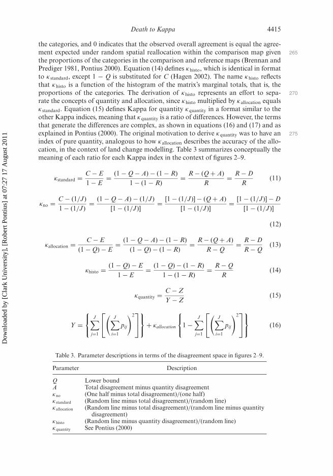
the categories, and 0 indicates that the observed overall agreement is equal the agree-ment expected under random spatial reallocation within the comparison map given 265

the proportions of the categories in the comparison and reference maps (Brennan andPrediger 1981, Pontius 2000). Equation (14) defines κhisto, which is identical in formatto κstandard, except 1 − Q is substituted for C (Hagen 2002). The name κhisto reflectsthat κhisto is a function of the histogram of the matrix’s marginal totals, that is, theproportions of the categories. The derivation of κhisto represents an effort to sepa- 270

rate the concepts of quantity and allocation, since κhisto multiplied by κallocation equalsκstandard. Equation (15) defines Kappa for quantity κquantity in a format similar to theother Kappa indices, meaning that κquantity is a ratio of differences. However, the termsthat generate the differences are complex, as shown in equations (16) and (17) and asexplained in Pontius (2000). The original motivation to derive κquantity was to have an 275

index of pure quantity, analogous to how κallocation describes the accuracy of the allo-cation, in the context of land change modelling. Table 3 summarizes conceptually themeaning of each ratio for each Kappa index in the context of figures 2–9.

κstandard = C − E1 − E

= (1 − Q − A) − (1 − R)1 − (1 − R)

= R − (Q + A)R

= R − DR

(11)

κno = C − (1/J)1 − (1/J)

= (1 − Q − A) − (1/J)[1 − (1/J)]

= [1 − (1/J)] − (Q + A)[1 − (1/J)]

= [1 − (1/J)] − D[1 − (1/J)]

(12)

κallocation = C − E(1 − Q) − E

= (1 − Q − A) − (1 − R)(1 − Q) − (1 − R)

= R − (Q + A)R − Q

= R − DR − Q

(13)

κhisto = (1 − Q) − E1 − E

= (1 − Q) − (1 − R)1 − (1 − R)

= R − QR

(14)

κquantity = C − ZY − Z

(15)

Y =⎧⎨⎩

J∑j=1

⎡⎣( J∑

i=1

pij

)2⎤⎦⎫⎬⎭+ κallocation

⎧⎨⎩1 −

J∑j=1

⎡⎣( J∑

i=1

pij

)2⎤⎦⎫⎬⎭ (16)

Table 3. Parameter descriptions in terms of the disagreement space in figures 2–9.

Parameter Description

Q Lower boundA Total disagreement minus quantity disagreementκno (One half minus total disagreement)/(one half)κ standard (Random line minus total disagreement)/(random line)κallocation (Random line minus total disagreement)/(random line minus quantity

disagreement)κhisto (Random line minus quantity disagreement)/(random line)κquantity See Pontius (2000)

Dow

nloa

ded

by [

Cla

rk U

nive

rsity

], [

Rob

ert P

ontiu

s] a

t 07:

27 1

7 A

ugus

t 201

1


Z = (1/J) + κallocation

⎧⎨⎩

J∑j=1

min

[(1/J),

J∑i=1

pij

]− (1/J)

⎫⎬⎭ (17)

2.5 Application to published matrices

All the parameters in this article derive entirely from the cross-tabulation matrix, so 280

we can compute the statistics easily for cases where authors publish their matrices.We compute the two components of disagreement and the standard Kappa index ofagreement for five examples taken from two articles in the International Journal ofRemote Sensing to show how the concepts work in practice.

Ruelland et al. (2008) analysed six categories in West Africa for three points in time: 285

1975, 1985 and 2000. The comparison maps derived from Landsat data and a recursivethresholding algorithm that seeks to maximize overall accuracy and κstandard. The ref-erence data consist of control points that were selected based on practical criteria, suchas being invariant since the 1970s and being close to trails. The article does not containsufficient information to understand whether the sample is representative of the pop- 290

ulation, and the authors performed no conversion from the observed sample matricesto estimated population matrices. The article does not report any Kappa indices. Thearticle reports per cent agreement in terms that imply that the overall percentage ofthe reference data that disagrees with the map of 1975, 1985 and 2000 is, respectively,24, 28 and 21. The article then analyses the net quantity differences among the maps’ 295

categories over the three years, and reports that there is 4.5% net quantity differencebetween the map of 1985 and 2000. Thus the reported overall error in each map isabout five times larger than the size of the reported difference between the maps. Thearticle states ‘results indicate relatively good agreement between the classifications andthe field observations’ (pp. 3542–3543), but the article never defines a criterion for rel- 300

atively good. Our results section below reveals the insight that is possible when oneexamines the two components of disagreement.

Wundram and Löffler (2008) analyse five categories in the Norwegian mountainsusing two matrices that derive from a supervised method and an unsupervised methodof classification. The article reports that 256 reference data points were collected ran- 305

domly, in which case the summary statistics that derive from the sample matrices areunbiased. The article reports κstandard for each method and interprets κstandard by say-ing that the value is higher for the unsupervised method, which the reported overallproportion correct already reveals. The article’s tables show 34% error for the super-vised classification and 23% error for the unsupervised classification, and the article 310

reports, ‘The results of supervised and unsupervised vegetation classification were notconsistently good’ (p. 969), but the article never defines a quantitative criterion fornot consistently good. The results section compares Wundram and Löffler (2008) toRuelland et al. (2008) with respect to components of disagreement and κstandard.

3. Results 315

3.1 Fundamental concepts

We analyse figure 1 by plotting results in a space similar to figure 2. In figures 3–9,the vertical axis is the proportion disagreement between the comparison map and thereference map, the horizontal axis is the proportion black in the comparison map and

Dow

nloa

ded

by [

Cla

rk U

nive

rsity

], [

Rob

ert P

ontiu

s] a

t 07:

27 1

7 A

ugus

t 201

1

Death to Kappa 4417

each number plotted in the space is an index’s value for a particular comparison map. 320

Q from equation (3) defines the quantity disagreement boundary, R from equation(10) defines the random allocation line and D from equation (4) defines the verticalcoordinate for the plotted value for each comparison map. The value at coordinates(0.22, 0.33) is the highlighted comparison map from figure 1, which we use to helpto explain the results. Figure 3 shows the quantity disagreement Q plotted in this 325

space. There is a column of zeros where the quantity in the black category is one third,because the reference map has three black pixels among its nine pixels. The numberswithin each column are identical in figure 3 because the quantity disagreement is dic-tated completely by the proportion of the black category in each comparison map.

1.0

0.9

0.8

0.7

0.6

0.5

To

tal d

isa

gre

em

en

t (p

rop

ort

ion

)

0.4

0.3

0.2

0.1

0.0

0.0 0.1 0.2 0.3 0.4

Quantity of black category in comparison map (proportion)

0.5 0.6 0.7 0.8 0.9 1.0

0.33

0.33

0.33

0.33

0.22

0.33

0.22

0.22

0.220.22

0.22

0.11

0.11

0.110.11

0.11

0.11

maximum disagreement

random allocation

quantity disagreement

0.11

0.00

0.00

0.00

0.00

0.44

0.44

0.44

0.56

0.56

0.67

Figure 3. Quantity disagreement Q shown by the values plotted in the space.

1.0

0.9

0.8

0.7

0.6

0.5

Tota

l dis

ag

reem

ent

(pro

port

ion)

0.4

0.22

0.22

0.22

0.00

0.00

0.00

0.00

0.00

0.00

0.00

0.00

0.00

0.00 0.22

0.22

0.22

0.22

0.22

0.44

0.440.44

0.44

0.44

0.44

0.67

0.67

0.67

0.67

0.3

0.2

0.1

0.0

0.0 0.1 0.2 0.3 0.4


0.5 0.6 0.7 0.8 0.9 1.0


random allocation


Figure 4. Allocation disagreement A shown by the values plotted in the space.

Dow

nloa

ded

by [

Cla

rk U

nive

rsity

], [

Rob

ert P

ontiu

s] a

t 07:

27 1

7 A

ugus

t 201

1


Figure 4 shows the allocation disagreement A, which measures the distance above the 330

quantity disagreement boundary. Quantity disagreement and allocation disagreementsum to the total disagreement D.

Figure 5 shows results for κstandard. Values are positive below the random allocationline, 0 on the line and negative above the line, by design of the formula for κstandard.The highlighted comparison map in figure 1 has κstandard = 0.18, which is a ratio with 335

a numerator of 0.41–0.33 and a denominator of 0.41, according to equation (11) andthe vertical intervals between the left ends of the braces in figure 5. A single row ofnumbers in figure 5 contains different values for κstandard, which indicates that κstandard

does not give the same result for comparison maps that have the same amount oftotal disagreement with the reference map. For example, κstandard ranges from −0.36 to 340

0.12, when total disagreement is 0.56, that is, when five of the nine pixels disagree. Thisrange shows how κstandard can indicate allocation disagreement more than quantity dis-agreement. The value of −0.36 shows how κstandard does not reward for small quantitydisagreement and penalizes strongly for allocation disagreement, and the 0.12 showshow κstandard does not penalize strongly for large quantity disagreement and rewards 345

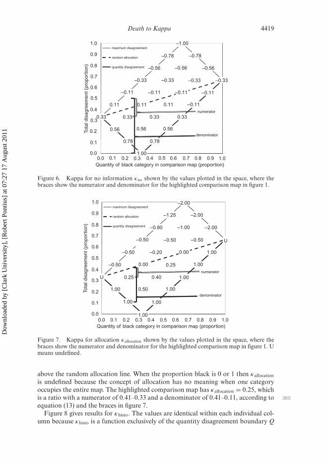
for small allocation disagreement (Pontius 2000).Figure 6 gives κno, which indicates where the comparison maps’ total disagreement

is relative to 1/J, which is 0.5 in the case study that has two categories. If disagree-ment is 0, then κno is 1; if disagreement is <0.5, then κno is positive; if disagreementis >0.5, then κno is negative. κno has the same value within any given row of num- 350

bers in figure 6 because κno is a linear function of total disagreement. The highlightedcomparison map has κno = 0.33, which is a ratio with a numerator of 0.50–0.33 and adenominator of 0.50, according to equation (12) and the vertical intervals within thebraces of figure 6.

Figure 7 gives κallocation. If allocation disagreement is 0, then κallocation is 1. κallocation is 355

positive below the random allocation line, 0 on the random allocation line and negative

1.0

0.9

0.8

0.7

0.6

0.5

Tota

l dis

ag

reem

ent

(pro

port

ion)

0.4

0.3

0.40

0.73 0.77

0.57

0.40

0.00

0.00

0.00 0.18

0.14

0.31

0.50

0.25

numerator

denominator

0.12

0.00

–0.24–0.40

–0.13

–0.50

–0.80

–0.71

–0.62

–0.50

–0.36

–0.20

–0.15

–0.29

1.00

0.2

0.1

0.0

0.0 0.1 0.2 0.3 0.4


0.5 0.6 0.7 0.8 0.9 1.0


random allocation


Figure 5. Standard Kappa κ standard shown by the values plotted in the space, where the bracesshow the numerator and denominator for the highlighted comparison map in figure 1.

Dow

nloa

ded

by [

Cla

rk U

nive

rsity

], [

Rob

ert P

ontiu

s] a

t 07:

27 1

7 A

ugus

t 201

1

Death to Kappa 4419

1.0

0.9

0.8

0.7

0.6

0.5

To

tal dis

ag

reem

ent

(pro

port

ion)

0.40.11

–0.11 –0.11

–1.00

–0.78–0.78

–0.56–0.56

–0.33 –0.33

–0.11 –0.11

–0.110.110.11

0.33 0.330.33

0.560.56 0.56

0.780.78

1.00

0.33

–0.33–0.33

–0.56

0.3

numerator

denominator0.2

0.1

0.00.0 0.1 0.2 0.3 0.4


0.5 0.6 0.7 0.8 0.9 1.0


random allocation


Figure 6. Kappa for no information κno shown by the values plotted in the space, where thebraces show the numerator and denominator for the highlighted comparison map in figure 1.

1.0

0.9

0.8

0.7

0.6

0.5

To

tal d

isa

gre

em

en

t (p

rop

ort

ion

)

0.4

0.3

0.2

0.1

0.0

0.0 0.1 0.2 0.3 0.4


0.5 0.6 0.7 0.8 0.9 1.0


random allocation


–2.00

–0.50 –0.50

–0.20

–2.00

–2.00

–1.00

–1.25

–0.80

–0.50

–0.50

–0.50

U

U

0.50

1.00

1.00

1.001.00

1.00

1.00

1.00

0.40

0.00

0.00

1.00

0.25

0.25numerator

denominator

Figure 7. Kappa for allocation κallocation shown by the values plotted in the space, where thebraces show the numerator and denominator for the highlighted comparison map in figure 1. Umeans undefined.

above the random allocation line. When the proportion black is 0 or 1 then κallocation

is undefined because the concept of allocation has no meaning when one categoryoccupies the entire map. The highlighted comparison map has κallocation = 0.25, whichis a ratio with a numerator of 0.41–0.33 and a denominator of 0.41–0.11, according to 360

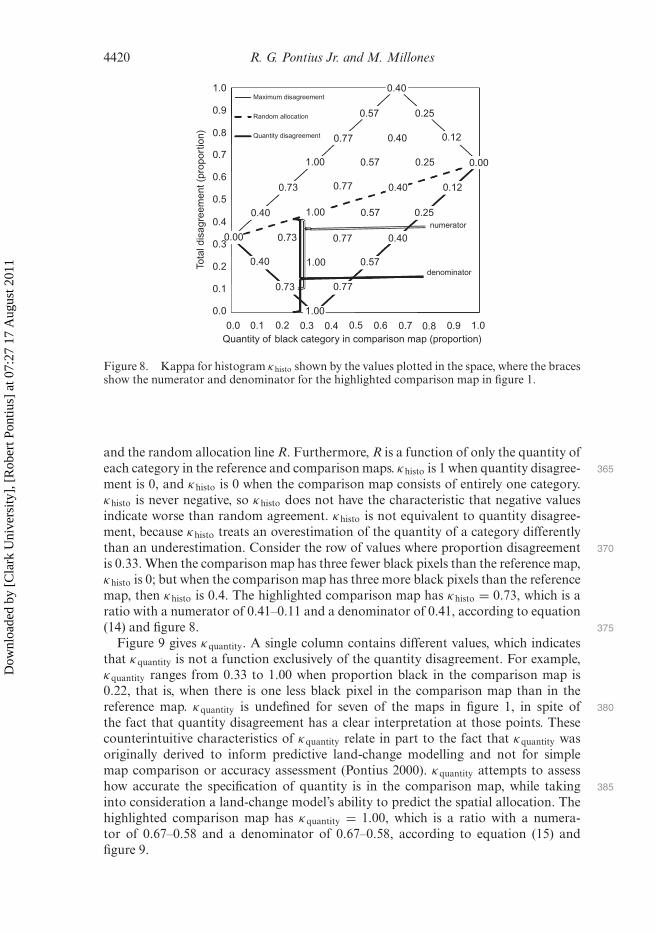
equation (13) and the braces in figure 7.Figure 8 gives results for κhisto. The values are identical within each individual col-

umn because κhisto is a function exclusively of the quantity disagreement boundary Q

Dow

nloa

ded

by [

Cla

rk U

nive

rsity

], [

Rob

ert P

ontiu

s] a

t 07:

27 1

7 A

ugus

t 201

1


1.0

0.9

0.8

0.7

0.6

0.5To

tal dis

ag

reem

ent

(pro

port

ion)

0.4

0.3

0.2

0.1

0.0

0.0 0.1 0.2 0.3 0.4


0.5 0.6 0.7 0.8 0.9 1.0

Maximum disagreement

Random allocation


0.40

0.40

0.40

0.73

0.73

0.40

0.40

0.73

0.25

0.25

0.25

0.40

1.00

0.12

0.00

0.00

1.00

1.00

1.00

0.12

0.57

0.77

0.77

0.57

0.57

0.57

0.77

0.77

numerator

denominator

Figure 8. Kappa for histogram κhisto shown by the values plotted in the space, where the bracesshow the numerator and denominator for the highlighted comparison map in figure 1.

and the random allocation line R. Furthermore, R is a function of only the quantity ofeach category in the reference and comparison maps. κhisto is 1 when quantity disagree- 365

ment is 0, and κhisto is 0 when the comparison map consists of entirely one category.κhisto is never negative, so κhisto does not have the characteristic that negative valuesindicate worse than random agreement. κhisto is not equivalent to quantity disagree-ment, because κhisto treats an overestimation of the quantity of a category differentlythan an underestimation. Consider the row of values where proportion disagreement 370

is 0.33. When the comparison map has three fewer black pixels than the reference map,κhisto is 0; but when the comparison map has three more black pixels than the referencemap, then κhisto is 0.4. The highlighted comparison map has κhisto = 0.73, which is aratio with a numerator of 0.41–0.11 and a denominator of 0.41, according to equation(14) and figure 8. 375

Figure 9 gives κquantity. A single column contains different values, which indicatesthat κquantity is not a function exclusively of the quantity disagreement. For example,κquantity ranges from 0.33 to 1.00 when proportion black in the comparison map is0.22, that is, when there is one less black pixel in the comparison map than in thereference map. κquantity is undefined for seven of the maps in figure 1, in spite of 380

the fact that quantity disagreement has a clear interpretation at those points. Thesecounterintuitive characteristics of κquantity relate in part to the fact that κquantity wasoriginally derived to inform predictive land-change modelling and not for simplemap comparison or accuracy assessment (Pontius 2000). κquantity attempts to assesshow accurate the specification of quantity is in the comparison map, while taking 385

into consideration a land-change model’s ability to predict the spatial allocation. Thehighlighted comparison map has κquantity = 1.00, which is a ratio with a numera-tor of 0.67–0.58 and a denominator of 0.67–0.58, according to equation (15) andfigure 9.

Dow

nloa

ded

by [

Cla

rk U

nive

rsity

], [

Rob

ert P

ontiu

s] a

t 07:

27 1

7 A

ugus

t 201

1

Death to Kappa 4421

1.0

0.9

0.8

numerator

and

denominator

0.7

0.6U

U

U

U

0.33

U

0.33

1.00

–0.33

0.33

–0.33

–1.00

–1.67

–1.00 –2.33

–2.33

–1.67–0.33

–1.00

–1.00

–0.33

0.33

U

1.00

0.331.00

U

1.00

0.5

To

tal dis

ag

reem

ent

(pro

port

ion)

0.4

0.3

0.2

0.1

0.00.0 0.1 0.2 0.3 0.4


0.5 0.6 0.7 0.8 0.9 1.0

Figure 9. Kappa for quantity κquantity shown by the values plotted in the space, where thebraces show the numerator and denominator for the highlighted comparison map in figure 1.U means undefined.

3.2 Applications to peer-reviewed literature 390

Figure 10 shows the two components of disagreement and κstandard for five matri-ces in peer-reviewed literature. The two components of disagreement are stacked toshow how they sum to the total disagreement. Thus the figure conveys informationabout proportion correct, since proportion correct is 1 minus the total proportiondisagreement. 395

The results for Ruelland et al. (2008) show that the relative ranking of κstandard isidentical to the relative ranking of proportion correct among their three matrices,which demonstrates how κstandard frequently conveys information that is redundantwith proportion correct. Each bar for Ruelland et al. (2008) also demonstrates thatquantity disagreement accounts for less than a quarter of the overall disagreement. 400

This is important because one of the main purposes of their research is to estimate thenet quantity of land-cover change among the three points in time, in which case alloca-tion disagreement is much less important than quantity disagreement. The separationof the overall disagreement into components of quantity and allocation reveals thattheir maps are actually much more accurate for their particular purpose than implied 405

by the reported overall errors of more than 20%. The κstandard indices do not offer thistype of insight.

Figure 10 demonstrates some additional characteristics of κstandard described above.Specifically, the Ruelland et al. (2008) application to 1985 has 25% total disagree-ment and the Wundram and Löffler (2008) application to the unsupervised case has 410

23% total disagreement, while κstandard for both is 0.65. κstandard fails to reveal thatthe Wundram and Löffler (2008) application to unsupervised classification has morequantity disagreement than the Ruelland et al. (2008) application to 1985. Quantitydisagreement accounts for more than a quarter of the total disagreement withinthe Wundram and Löffler (2008) application to unsupervised classification, which is 415

Dow

nloa

ded

by [

Cla

rk U

nive

rsity

], [

Rob

ert P

ontiu

s] a

t 07:

27 1

7 A

ugus

t 201

1


Ruelland et al. (2008)

1975


1985


2000

Wundram and Löffler (2008)

unsupervised

Wundram and Löffler (2008)

supervised

0.00 0.05 0.10 0.15 0.20 0.25 0.30 0.35

Disagreement (proportion of observations)

0.51

0.65

0.73

0.65

0.69

Quantity Allocation

Figure 10. Quantity disagreement, allocation disagreement and κ standard below each bar forfive matrices published in the International Journal of Remote Sensing.

important to know for practical applications, but κstandard is designed neither to penal-ize substantially for large quantity disagreement nor to reward substantially for smallquantity disagreement.

4. Discussion

4.1 Reasons to abandon Kappa 420

We have revealed several detailed reasons why it is more helpful to summarize thecross-tabulation matrix in terms of quantity disagreement and allocation disagree-ment, as opposed to proportion correct or the various Kappa indices. This discussionsection provides three main overarching rationales.

First, each Kappa index is a ratio, which can introduce problems in calculation and 425

interpretation. If the denominator is 0, then the ratio is undefined, so interpretation isdifficult or impossible. If the ratio is defined and large, then it is not immediately clearwhether the ratio’s size is attributable to a large numerator or a small denominator.Conversely, when the ratio is small, it is not clear whether the ratio’s size is attributableto a small numerator or a large denominator. In particular, κquantity can demonstrate 430

this problem, in some cases leading to nearly uninterpretable values of κquantity that are<−1 or >1 (Schneider and Pontius 2001). Kappa’s ratio is unnecessarily complicatedbecause usually the most relevant ingredient to Kappa is only one part of the numer-ator, that is, the total disagreement as seen in the right sides of equations (11)–(13).This total disagreement can be expressed as the sum of two components of quantity 435

disagreement and allocation disagreement in a much more interpretable manner thanKappa’s unitless ratio, since both components express a proportion of the study area.

Second, it is more helpful to understand the two components of disagreementthan to have a single summary statistic of agreement when interpreting results anddevising the next steps in a research agenda. The two components of disagreement 440

Dow

nloa

ded

by [

Cla

rk U

nive

rsity

], [

Rob

ert P

ontiu

s] a

t 07:

27 1

7 A

ugus

t 201

1

Death to Kappa 4423

begin to explain the reasons for the disagreement based on information in the matrix.Examination of the relative magnitudes of the components can be used to learn aboutsources of error. A statement that the overall Kappa is X or proportion correct is Pdoes not give guidance on how to improve the classification, since such statementsoffer no insight to the sources of disagreement. When one shifts focus from over- 445

all agreement to components of disagreement, it orients one’s mind in an importantrespect. For example, Ruelland et al. (2008) report that an agreement of 72% is good,while Wundram and Loffler (2008) report that a disagreement of 23% is not good.Perhaps they came to these conclusions because Ruelland et al. (2008) focused onagreement and Wundram and Loffler (2008) focused on disagreement. It is much 450

more common in the culture of remote sensing to report agreement than disagree-ment, which is unfortunate. If Ruelland et al. (2008) would have examined the twocomponents of disagreement, then they could have interpreted the accuracy of theirmaps relative to their research objective, which was to examine the differences amongmaps from three points in time. It is usually more helpful to focus on the disagreement 455

and to wonder how to explain the error, which is what the two components of disagree-ment do, rather than to focus on the agreement and to worry that randomness mightexplain some of the correctness, which is what the Kappa indices of agreement do.

Third, and most importantly, the Kappa indices attempt to compare observedaccuracy relative to a baseline of accuracy expected due to randomness, but in the 460

applications that we have seen, randomness is an uninteresting, irrelevant and/ormisleading baseline. For example, the κstandard addresses the question, ‘What is theobserved overall agreement relative to the statistically expected agreement that wewould obtain by random spatial reallocation of the categories within the comparisonmap, given the proportions of the categories in the comparison and reference maps, 465

regardless of the size of the quantity disagreement?’ κstandard answers this questionon a scale where 0 indicates that the observed agreement is equal to the statisticallyexpected agreement due to random spatial reallocation of the specified proportions ofthe categories, and 1 indicates that the observed agreement derives from perfect speci-fication of both the spatial allocation and the proportions of the categories. We cannot 470

think of a single application in remote sensing where it is necessary to know the answerto that question as measured on that scale in order to make a practical decision, espe-cially given that a simpler measure of accuracy, such as proportion correct, is alreadyavailable. We know of only two cases in land-change modelling where κallocation canbe somewhat helpful (Pontius et al. 2003, Pontius and Spencer 2005) because κallocation 475

answers that question on a scale where 0 indicates that the observed agreement is equalto the statistically expected agreement due to random spatial reallocation of the speci-fied proportions of the categories, and 1 indicates that the observed agreement is due tooptimal spatial allocation of the specified proportions of the categories. Furthermore,we know of no papers where the authors come to different conclusions when they 480

interpret proportion correct vis-à-vis κstandard, which makes us wonder why authorsusually present both proportion correct and κstandard.

We suspect the remote-sensing profession is enamoured with κstandard because thecomparison to a baseline of randomness, that is, chance, is a major theme in univer-sity courses concerning statistical theory, so the concept of κstandard sounds appealing 485

initially. However, comparison to randomness in statistical theory is important whensampling, but sampling is an entirely different concept than the selection of a param-eter to summarize a cross-tabulation matrix. The Kappa indices are parameters thatattempt to account for types of randomness that are conceptually different than therandomness due to sampling. Specifically, if the underlying matrix derives from a 490

Dow

nloa

ded

by [

Cla

rk U

nive

rsity

], [

Rob

ert P

ontiu

s] a

t 07:

27 1

7 A

ugus

t 201

1


sample of the population, then each different possible sample matrix (table 1) mightproduce a different estimated population matrix (table 2), which will lead to a differentstatistical value for a selected parameter. The sampling distribution for that parameterindicates the possible variation in the values due to the sampling procedure. We havenot yet derived the sampling distributions for quantity disagreement and allocation 495

disagreement, which is a potential topic for future work.

4.2 A more appropriate baseline

There is a clear need to have a baseline for an accuracy assessment of a particular clas-sified map. The unfortunate cultural problem in the remote-sensing community is that85% correct is frequently used as a baseline for a map to be considered good. It makes 500

no sense to have a universal standard for accuracy in practical applications (Foody2008), in spite of temptations to establish such standards (Landis and Koch 1977,Monserud and Leemans 1992) because a universal standard is not related to any spe-cific research question or study area. Perhaps some investigators think κstandard avoidsthis problem because randomness can generate a baseline value that reflects the partic- 505

ular case study. However, the use of any Kappa index assumes that randomization is anappropriate and important baseline. We think that randomness is usually not a reason-able baseline because a reasonable baseline should reflect the alternative second-bestmethod to generate the comparison map, and that second-best method is usually notrandomization. So, what is an appropriate baseline? The baseline should be related 510

to a second-best method to create the comparison map in a manner that uses thecalibration information for the particular study site in a quick and/or naïve approach.

For example, Wu et al. (2009) compared eight mathematically sophisticated meth-ods to generate a map of nine categories. If both quantity and allocation werepredicted randomly, then the completely random prediction would have a proportion 515

correct of 1/9 (Brennan and Prediger 1981, Foody 1992). However, the authors wiselydid not use this random value as a baseline. They intelligently used two naïve methodsto serve as baselines in a manner that considered how they separated calibration datafrom validation data. The calibration data consisted 89% of a single category. Thusone naïve baseline was to predict that all the validation points were that single cate- 520

gory, which produced a baseline with 11% quantity disagreement and zero allocationdisagreement. A second naïve baseline was to predict that each validation point wasthe same category as the nearest calibration point, which produced a second baselinewith almost zero quantity disagreement and 20% allocation disagreement. Only oneof the eight mathematically sophisticated methods was more accurate than both of the 525

naïve baselines, while seven of the eight sophisticated models were more accurate thana completely random prediction.

Pontius et al. (2007) presented an example from land change modelling in theAmazon where a naïve model predicted that deforestation occurs simply near the mainhighway, and a null model predicted that no deforestation occurs. Both the naïve and 530

the null models were more accurate than a prediction that deforestation occurs ran-domly in space. They concluded that the question ‘How is the agreement less thanperfect?’ is an entirely different and more relevant question than ‘Is the agreementbetter than random?’ The components of disagreement answer the more importantformer question, while the Kappa indices address the less important latter question. 535

The two components of disagreement have many applications regardless of whetherthe components derived from a sample of the population or from comparison of mapsthat have complete coverage. For example, Pontius et al. (2008a) show how to use the

Dow

nloa

ded

by [

Cla

rk U

nive

rsity

], [

Rob

ert P

ontiu

s] a

t 07:

27 1

7 A

ugus

t 201

1

Death to Kappa 4425

components for various types of map comparisons, while Pontius et al. (2008b) showhow to compute the components for maps of a continuous real variable. 540

5. Conclusions

This article reflects more than a decade of research on the Kappa indices of agreement.We have learned that the two simple measures of quantity disagreement and allocationdisagreement are much more useful to summarize a cross-tabulation matrix than thevarious Kappa indices for the applications that we have seen. We know of no cases in 545

remote sensing where the Kappa indices offer useful information because the Kappaindices attempt to compare accuracy to a baseline of randomness, but randomness isnot a reasonable alternative for map construction. Furthermore, some Kappa indiceshave fundamental conceptual flaws, such as being undefined even for simple cases, orhaving no useful interpretation. The first author apologizes for publishing some of the 550

variations of Kappa in 2000, and asks that the professional community does not usethem. Instead, we recommend that the profession adopt the two measures of quantitydisagreement and allocation disagreement, which are much simpler and more helpfulfor the vast majority of applications. These measurements can be computed easilyby entering the cross-tabulation matrix into a spreadsheet available free of charge at 555

http://www.clarku.edu/∼rpontius. These two measurements illuminate a much moreenlightened path, as we look forward to another decade of learning.

AcknowledgementsThe United States’ National Science Foundation (NSF) supported this work throughits Coupled Natural Human Systems program via grant BCS-0709685. NSF supplied 560

additional funding through its Long Term Ecological Research network via grantOCE-0423565 and a supplemental grant DEB-0620579. Any opinions, findings, con-clusions or recommendation expressed in this article are those of the authors and donot necessarily reflect those of the funders. Clark Labs produced the GIS softwareIdrisi, which computes the two components of disagreement that this article endorses. 565

Anonymous reviewers supplied constructive feedback that helped to improve thisarticle.

ReferencesAICKIN, M., 1990, Maximum likelihood estimation of agreement in the constant predictive

probability model, and its relation to Cohen’s kappa. Biometrics, 46, pp. 293–302. 570

ALLOUCHE, O., TSOAR, A. and KADMON, R., 2006, Assessing the accuracy of species distribu-tion models: prevalence, kappa and true skill statistic (TSS). Journal of Applied Ecology,43, pp. 1223–1232.

ALO, C. and PONTIUS JR., R.G., 2008, Identifying systematic land cover transitions usingremote sensing and GIS: the fate of forests inside and outside protected areas of 575

southwestern Ghana. Environment and Planning B, 435, pp. 280–295.BRENNAN, R. and PREDIGER, D., 1981, Coefficient kappa: some uses, misuses, and alternatives.

Educational and Psychological Measurement, 41, pp. 687–699.COHEN, J., 1960, A coefficient of agreement for nominal scales. Educational and Psychological

Measurement, 20, pp. 37–46. 580

CONGALTON, R.G., 1981, The use of discrete multivariate analysis for the assessment of Landsatclassification accuracy. MS thesis, Virginia Polytechnic Institute and State University,Blacksburg, VA, USA.

CONGALTON, R.G., 1991, A review of assessing the accuracy of classifications of remotely senseddata. Remote Sensing of Environment, 37, pp. 35–46. 585

Dow

nloa

ded

by [

Cla

rk U

nive

rsity

], [

Rob

ert P

ontiu

s] a

t 07:

27 1

7 A

ugus

t 201

1


CONGALTON, R.G. and GREEN, K., 1999, Assessing the Accuracy of Remotely Sensed Data:Principles and Practices (Boca Raton, FL: Lewis).

CONGALTON, R.G. and GREEN, K., 2009, Assessing the Accuracy of Remotely Sensed Data:Principles and Practices, 2nd ed. (Boca Raton, FL: CRC Press).

CONGALTON, R.G., ODERWALD, R.G. and MEAD, R.A., 1983, Assessing Landsat classification 590

accuracy using discrete multivariate analysis statistical techniques. PhotogrammetricEngineering and Remote Sensing, 49, pp. 1671–1678.

DI EUGENIO, B. and GLASS, M., 2004, The kappa statistic: a second look. ComputationalLinguistics, 30, pp. 95–101.

EASTMAN, J.R., 2009, IDRISI Taiga Tutorial. Accessed in IDRISI 16.05 (Worcester, MA: Clark 595

University).ERDAS INC, 2008, Field Guide, Vol. 2 (Norcross, GA: Erdas).FIELDING, A.H. and BELL, J.F., 1997, A review of methods for the assessment of predic-

tion errors in conservation presence/absence models. Environmental Conservation, 24,pp. 38–49. 600

FOODY, G.M., 1992, On the compensation for chance agreement in image classification accuracyassessment. Photogrammetric Engineering and Remote Sensing, 58, pp. 1459–1460.

FOODY, G.M., 2002, Status of land cover classification accuracy assessment. Remote Sensing ofEnvironment, 80, pp. 185–201.

FOODY, G.M., 2004, Thematic map comparison: evaluating the statistical significance of differ- 605

ences in classification accuracy. Photogrammetric Engineering and Remote Sensing, 70,pp. 627–633.

FOODY, G.M., 2008, Harshness in image classification accuracy assessment. InternationalJournal of Remote Sensing, 29, pp. 3137–3158.

GALTON, F., 1892, Finger Prints (London: Macmillan). 610

GERGEL, S.E. and TURNER, M.G. (Eds.), 2002, Learning Landscape Ecology: A Practical Guideto Concepts and Techniques (New York: Springer-Verlag).

GOODMAN, L.A. and KRUSKAL, W.H., 1954, Measures of association for cross classification.Journal of the American Statistical Association, 49, pp. 732–764.

HAGEN, A., 2002, Multi-method assessment of map similarity. In 5th Conference on Geographic 615

Information Science, 25–27 April 2002, Palma de Mallorca, Spain.HUDSON, W. and RAMM, C., 1987, Correct formulation of the kappa coefficient of agreement.

Photogrammetric Engineering and Remote Sensing, 53, pp. 421–422.JUNG, H.-W., 2003, Evaluating interrater agreement in SPICE-based assessments. Computer

Standards and Interfaces, 25, pp. 477–499. 620

LANDIS, J. and KOCH, G., 1977, The measurement of observer agreement for categorical data.Biometrics, 33, pp. 159–174.

LIU, C., FRAZIERB, P. and KUMA, L., 2007, Comparative assessment of the measures ofthematic classification accuracy. Remote Sensing of Environment, 107, pp. 606–616.

MA, Z. and REDMOND, R.L., 1995, Tau coefficients for accuracy assessment of classifica- 625

tion of remote sensing data. Photogrammetric Engineering and Remote Sensing, 61,pp. 435–439.

MONSERUD, R.A. and LEEMANS, R., 1992, Comparing global vegetation maps with the kappastatistic. Ecological Modelling, 62, pp. 275–293.

PONTIUS JR, R.G., 2000, Quantification error versus location error in comparison of categorical 630

maps. Photogrammetric Engineering and Remote Sensing, 66, pp. 1011–1016.PONTIUS JR, R.G., 2002, Statistical methods to partition effects of quantity and location during

comparison of categorical maps at multiple resolutions. Photogrammetric Engineeringand Remote Sensing, 68, pp. 1041–1049.

PONTIUS JR, R.G., AGRAWAL, A. and HUFFAKER, D., 2003, Estimating the uncertainty of 635

land-cover extrapolations while constructing a raster map from tabular data. Journalof Geographical Systems, 5, pp. 253–273.

PONTIUS JR, R.G., BOERSMA, W., CASTELLA, J.-C., CLARKE, K., DE NIJS, T., DIETZEL, C.,DUAN, Z., FOTSING, E., GOLDSTEIN, N., KOK, K., KOOMEN, E., LIPPITT, C.D.,

Dow

nloa

ded

by [

Cla

rk U

nive

rsity

], [

Rob

ert P

ontiu

s] a

t 07:

27 1

7 A

ugus

t 201

1

Death to Kappa 4427

MCCONNELL, W., MOHD SOOD, A., PIJANOWSKI, B., PITHADIA, S., SWEENEY, S., 640

TRUNG, T.N., VELDKAMP, A.T. and VERBURG, P.H., 2008a, Comparing the input,output, and validation maps for several models of land change. The Annals of RegionalScience, 42, pp. 11–47.

PONTIUS JR, R.G., SHUSAS, E. and MCEACHERN, M., 2004, Detecting important cate-gorical land changes while accounting for persistence. Agriculture, Ecosystems and 645

Environment, 101, pp. 251–268.PONTIUS JR, R.G. and SPENCER, J., 2005, Uncertainty in extrapolations of predictive land

change models. Environment and Planning B: Planning and Design, 32, pp. 211–230.PONTIUS JR, R.G. and SUEDMEYER, B., 2004, Components of agreement between categorical

maps at multiple resolutions. In Remote Sensing and GIS Accuracy Assessment, R.S. 650

Lunetta and J.G. Lyon (Eds.), pp. 233–251 (Boca Raton, FL: CRC Press).PONTIUS JR, R.G., THONTTEH, O. and CHEN, H., 2008b, Components of information for mul-

tiple resolution comparison between maps that share a real variable. Environmental andEcological Statistics, 15, pp. 111–142.

PONTIUS JR, R.G., WALKER, R.T., YAO-KUMAH, R., ARIMA, E., ALDRICH, S., CALDAS, M. 655

and VERGARA, D., 2007, Accuracy assessment for a simulation model of Amazoniandeforestation. Annals of the Association of American Geographers, 97, pp. 677–695.

REMMEL, T.K., 2009, Investigating global and local categorical map configuration comparisonsbased on coincidence matrices. Geographical Analysis, 41, pp. 113–126.

ROSENFIELD, G. and FITZPATRICK-LINS, K., 1986, A coefficient of agreement as a measure of 660

thematic classification accuracy. Photogrammetric Engineering and Remote Sensing, 52,pp. 223–227.

RUELLAND, D., DEZETTER, A., PUECH, C. and ARDOIN-BARDIN, S., 2008, Long-term monitor-ing of land cover changes based on Landsat imagery to improve hydrological modellingin West Africa. International Journal of Remote Sensing, 29, pp. 3533–3551. 665

SCHNEIDER, L. and PONTIUS JR, R.G., 2001, Modeling land-use change in the Ipswichwatershed, Massachusetts, USA. Agriculture, Ecosystems and Environment, 85,pp. 83–94.

SCOTT, W.A., 1955, Reliability of content analysis: the case of nominal scale coding. PublicOpinion Quarterly, 19, pp. 321–325. 670

SMITS, P.C., DELLEPIANE, S.G. and SCHOWENGERDT, R.A., 1999, Quality assessment of imageclassification algorithms for land-cover mapping: a review and proposal for a cost-basedapproach. International Journal of Remote Sensing, 20, pp. 1461–1486.

STEHMAN, S.V., 1997, Selecting and interpreting measures of thematic classification accuracy.Remote Sensing of Environment, 62, pp. 77–89. 675

STEHMAN, S.V., 2009, Sampling designs for accuracy assessment of land cover. InternationalJournal of Remote Sensing, 30, pp. 5243–5272.

STEHMAN, S.V. and CZAPLEWSKI, R.L., 1998, Design and analysis for thematic mapaccuracy assessment: fundamental principles. Remote Sensing of Environment, 64,pp. 331–344. 680

TURK, G., 2002, Map evaluation and ‘chance correction’. Photogrammetric Engineering andRemote Sensing, 68, pp. 123–133.

VISSER, H. and DE NIJS, T., 2006, The map comparison kit. Environmental Modeling andSoftware, 21, pp. 346–358.

WILKINSON, G.G., 2005, Results and implications of a study of fifteen years of satellite image 685

classification experiments. IEEE Transactions on Geoscience and Remote Sensing, 43,pp. 433–440.

WU, S., XIAOMIN, Q., USERY, E.L. and WANG, L., 2009, Using geometrical, textural, and con-textual information of land parcels for classifying detailed urban land use. Annals of theAssociation of American Geographers, 99, pp. 76–98. 690

WUNDRAM, D. and LÖFFER, J., 2008, High-resolution spatial analysis of mountain landscapesusing a low-altitude remote sensing approach. International Journal of Remote Sensing,29, pp. 961–974.

Dow

nloa

ded

by [

Cla

rk U

nive

rsity

], [

Rob

ert P

ontiu

s] a

t 07:

27 1

7 A

ugus

t 201

1


Appendix

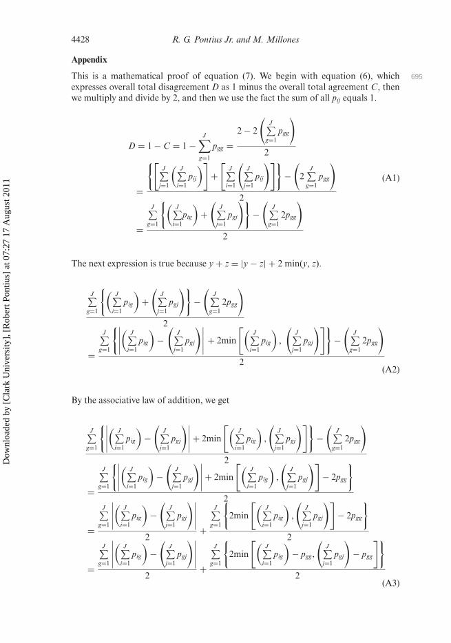
This is a mathematical proof of equation (7). We begin with equation (6), which 695

expresses overall total disagreement D as 1 minus the overall total agreement C, thenwe multiply and divide by 2, and then we use the fact the sum of all pij equals 1.

D = 1 − C = 1 −J∑

g=1

pgg =2 − 2

(J∑

g=1pgg

)

2

=

{[J∑

j=1

(J∑

i=1pij

)]+[

J∑i=1

(J∑

j=1pij

)]}−(

2J∑

g=1pgg

)

2

=

J∑g=1

{(J∑

i=1pig

)+(

J∑j=1

pgj

)}−(

J∑g=1

2pgg

)

2

(A1)

The next expression is true because y + z = |y − z| + 2 min(y, z).

J∑g=1

{(J∑

i=1pig

)+(

J∑j=1

pgj

)}−(

J∑g=1

2pgg

)

2

=

J∑g=1

{∣∣∣∣∣(

J∑i=1

pig

)−(

J∑j=1

pgj

)∣∣∣∣∣ + 2min

[(J∑

i=1pig

),

(J∑

j=1pgj

)]}−(

J∑g=1

2pgg

)

2(A2)

By the associative law of addition, we get

J∑g=1

{∣∣∣∣∣(

J∑i=1

pig

)−(

J∑j=1

pgj

)∣∣∣∣∣+ 2min

[(J∑

i=1pig

),

(J∑

j=1pgj

)]}−(

J∑g=1

2pgg

)

2

=

J∑g=1

{∣∣∣∣∣(

J∑i=1

pig

)−(

J∑j=1

pgj

)∣∣∣∣∣+ 2min

[(J∑

i=1pig

),

(J∑

j=1pgj

)]− 2pgg

}

2

=

J∑g=1

∣∣∣∣∣(

J∑i=1

pig

)−(

J∑j=1

pgj

)∣∣∣∣∣2

+

J∑g=1

{2min

[(J∑

i=1pig

),

(J∑

j=1pgj

)]− 2pgg

}

2

=

J∑g=1

∣∣∣∣∣(

J∑i=1

pig

)−(

J∑j=1

pgj

)∣∣∣∣∣2

+

J∑g=1

{2min

[(J∑

i=1pig

)− pgg,

(J∑

j=1pgj

)− pgg

]}

2(A3)

Dow

nloa

ded

by [

Cla

rk U

nive

rsity

], [

Rob

ert P

ontiu

s] a

t 07:

27 1

7 A

ugus

t 201

1

Death to Kappa 4429

Finally, by equations (2)–(5), we get 700

J∑g=1

∣∣∣∣∣(

J∑i=1

pig

)−(

J∑j=1

pgj

)∣∣∣∣∣2

+

J∑g=1

{2min

[(J∑

i=1pig

)− pgg,

(J∑

j=1pgj

)− pgg

]}

2

=

J∑g=1

qg

2+

J∑g=1

ag

2= Q + A

(A4)

Dow

nloa

ded

by [

Cla

rk U

nive

rsity

], [

Rob

ert P

ontiu

s] a

t 07:

27 1

7 A

ugus

t 201

1

Death to Kappa: birth of quantity disagreement and allocation disagreement for accuracy assessment

Documents