Deane Yang

MATH-UA 123 Calculus 3:Line Integrals, Fundamental Theorem of Line Integrals

Deane Yang

Courant Institute of Mathematical SciencesNew York University

November 8, 2021

LIVE TRANSCRIPT

START RECORDING

Parameterized Curves

I Recall that a parameterized curve is a map from an interval into 2-spaceor 3-space,

c : I → Rn, where n = 2 or 3

I The velocity of c is ~v(t) = c ′(t)

I We will assume that the velocity is always nonzero

I The path of the curve is the image of c

I A path has many different parameterizations

I The parameterized curves

c1(t) = (t, 0), 0 ≤ t ≤ 1

c2(t) = (t, 0), 0 ≤ t ≤ 1

c3(t) = (1− t, 0), 0 ≤ t ≤ 1

have the same path

Same Path, Different Parameterizations

I c1 : [0, 1]→ R2, wherec1(s) = s

I c1 : [−1, 0]→ R2, wherec1(s) = −s

I c1 : [0, 1]→ R2, wherec1(s) = 1− s

I c1 : [0, 1]→ R2, wherec1(s) = s2

Oriented Curve

end = c(b)

start = c(a)

start = c(b)

end = c(a)

I Orientation of a parameterized curve is direction of travelI There are two possible orientations

I The direction of the velocity vectorI The opposite direction to the velocity vector

I Consider a curve c : [a, b]→ Rn

I If the orientation is in the direction of the velocity vector c ′(t), then c(a)is the start point and c(b) is the end point

I If the orientation is in the opposite direction of the velocity vector c ′(t),then c(b) is the start point and c(a) is the end point

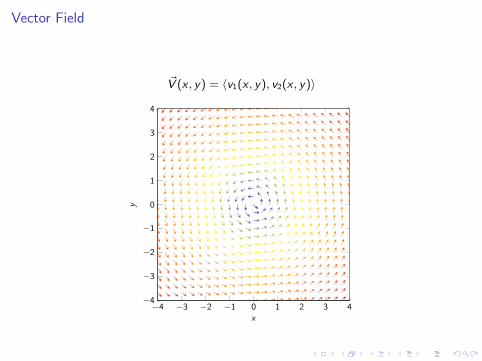
Vector Field

~V (x , y) = 〈v1(x , y), v2(x , y)〉

−4 −3 −2 −1 0 1 2 3 4−4

−3

−2

−1

0

1

2

3

4

x

y

Oriented Curve in Vector Field

~r(t) = 〈x(t), y(t)〉, a ≤ t ≤ b

−4 −3 −2 −1 0 1 2 3 4−4

−3

−2

−1

0

1

2

3

4

x

y

Oriented Curve in Vector FieldI Chop interval [a, b] into N equal pieces

∆t =b − a

NI

a = t1 < t2 = t1+∆t < · · · < tN = t1+(N−1)∆t < tN+1 = t1+(N+1)∆t = b

I Linear approximation of curve

~r(tk)− ~r(tk−1) ' ~r ′(tk)(tk − tk−1)

−4 −3 −2 −1 0 1 2 3 4−4

−3

−2

−1

0

1

2

3

4

x

y

Line Integral of Vector Field Along Oriented Curve

I Let C be a curve in a domain D with parameterization ~r(t), for each tbetween a and b

I Let ~V be a vector field on the domain D

I Define the line integral of a vector field ~V along an oriented curve C to be∫C

~V · d~r ' ~V (~r(t1)) · (~r(t2)− ~r(t1)) + · · ·+ ~V (~r(tN)) · (~r(tN+1)− ~r(tN))

' ~V (~r(t1)) · ~r ′(t1)(t2 − t1) + · · ·+ ~V (~r(tN)) · (~r ′(tN)(tN+1 − tN)

→∫ t=b

t=a

~V (~r(t)) · ~r ′(t) dt,

~r(t1)

~r(t2) ~r(t3)

~r(t4)

~V (~r(t1))

~V (~r(t2))~V (~r(t3))

~V (~r(t4))

I Does not matter whether a ≤ b or a ≥ b

Line integral of a Vector Field Along an Oriented Curve

I Let ~F (x , y , z) be a vector field on a domain D

I Let C an oriented curve in D with start point ~rstart and end point ~rend

I Let ~r(t) be a parameterization of C such that

~r(tstart) = ~rstart and ~r(tend) = ~rend

I The line integral of ~F along the curve C is defined to be∫C

~F · d~r =

∫ t=tend

t=tstart

~F (~r(t)) · ~r ′(t) dt

I Here, ~F = ~F (~r(t)) and d~r = ~r ′(t) dt

Examples

Calculation of Line Integral in Constant Vector Field

I Consider a constant vector field ~F = ~iF1 + ~jF2 + ~kF3, where F1,F2,F3 arescalar constants

I An oriented curve C with parameterization ~r(t) = ~ix(t) + ~jy(t) + ~jz(t),a ≤ t ≤ b, oriented in the direction of the velocity vectorI d~r = ~r ′(t) dt = (~ix ′(t) + ~jy ′(t) + ~kz ′(t)) dt

I We want to compute the line integral of ~F along the oriented curve C∫C

~F · d~r =

∫ t=b

t=a

〈F1,F2,F3〉〈x ′(t), y ′(t), z ′(t)〉 dt

=

∫ t=b

t=a

F1x′(t) + F2y

′(t) + F3z′(t) dt

= F1x(t) + F2y(t) + F3z(t)|t=bt=a

= F1(x(b)− x(a)) + F2(y(b)− y(a)) + F3(z(b)− z(a))

= ~F · (~r(b)− ~r(a))

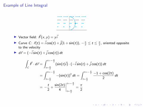
Example of Line Integral

I Vector field: ~F (x , y) = y~i

I Curve C : ~r(t) = ~i cos(t) + ~j(1 + sin(t)), −π2≤ t ≤ π

2, oriented opposite

to the velocity

I d~r = (−~i sin(t) + ~j cos(t)) dt∫C

~F · d~r =

∫ t=−π2

t=π2

(sin(t)~i) · (−~i sin(t) + ~j cos(t)) dt

=

∫ t=−π2

t=π2

−(sin(t))2 dt =

∫ t=−π2

t=π2

−1 + cos(2t)

2dt

= − t

2+

sin(2t)

4

∣∣∣∣t=−π2

t=π2

=π

2

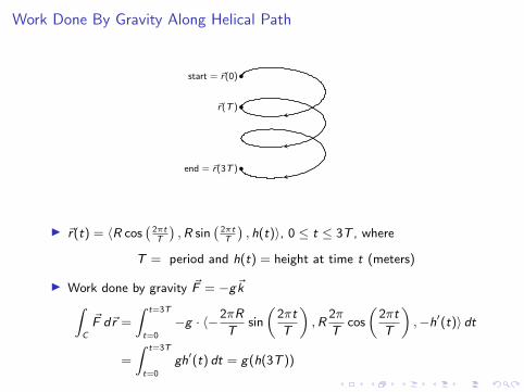
Work Done By Gravity Along Helical Path

end = ~r(3T )•

•start = ~r(0)

~r(T )•

I ~r(t) = 〈R cos(2πtT

),R sin

(2πtT

), h(t)〉, 0 ≤ t ≤ 3T , where

T = period and h(t) = height at time t (meters)

I Work done by gravity ~F = −g~k∫C

~F d~r =

∫ t=3T

t=0

−g · 〈−2πR

Tsin

(2πt

T

),R

2π

Tcos

(2πt

T

),−h′(t)〉 dt

=

∫ t=3T

t=0

gh′(t) dt = g(h(3T ))

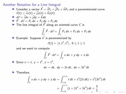
Another Notation for a Line IntegralI Consider a vector ~F = ~iF1 + ~jF2 + ~kF3 and a parameterized curve~r(t) = ~ix(t) + ~jy(t) + ~kz(t)

I d~r = ~idx + ~jdy + ~kdzI ~F · d~r = F1 dx + F2 dy + F3 dzI The line integral of ~F along an oriented curve C is∫

C

~F · d~r =

∫C

F1 dx + F2 dy + F3 dz

I Example: Suppose C is parameterized by

~r(t) = 〈t, t2, t3〉, 0 ≤ t ≤ 1

and we want to compute∫C

~F · d~r =

∫C

x dx + y dy + z dz

I Since x = t, y = t2, z = t3,

dx = dt, dy = 2t dt, dz = 3t2 dt

I Therefore,∫C

x dx + y dy + z dz =

∫ t=1

t=0

t dt + t2(2t dt) + t3(3t2) dt

=

∫ t=1

t=0

(t + 2t3 + 3t5) dt =3

2

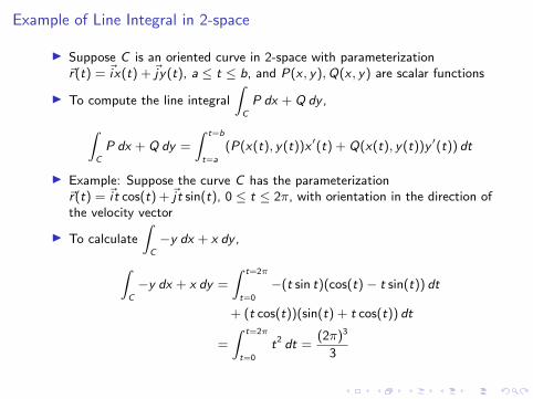
Example of Line Integral in 2-space

I Suppose C is an oriented curve in 2-space with parameterization~r(t) = ~ix(t) + ~jy(t), a ≤ t ≤ b, and P(x , y),Q(x , y) are scalar functions

I To compute the line integral

∫C

P dx + Q dy ,

∫C

P dx + Q dy =

∫ t=b

t=a

(P(x(t), y(t))x ′(t) + Q(x(t), y(t))y ′(t)) dt

I Example: Suppose the curve C has the parameterization~r(t) = ~i t cos(t) + ~jt sin(t), 0 ≤ t ≤ 2π, with orientation in the direction ofthe velocity vector

I To calculate

∫C

−y dx + x dy ,

∫C

−y dx + x dy =

∫ t=2π

t=0

−(t sin t)(cos(t)− t sin(t)) dt

+ (t cos(t))(sin(t) + t cos(t)) dt

=

∫ t=2π

t=0

t2 dt =(2π)3

3

Properties of Line Integrals

I If C is an oriented curve and ~F is a vector field, then the line integral of ~Falong C is ∫

C

~F · d~r =

∫ t=tend

t=tstart

~F (~r(t)) · ~r ′(t) dt,

where ~r(t) is a parameterization of C

I The value of the line integral stays the same, even if a differentparameterization is used

I Given an oriented curve C , −C will denote the same curve but with theopposite orientation: ∫

−C

~F · d~r = −∫C

~F · d~r

I If C = C1 ∪ C2, then∫C

~F · d~r =

∫C1

~F · d~r +

∫C2

~F · d~r

Gradient Field

I A vector field ~F a domain D is a gradient field, if there is a scalar functionf on D such that

~F = ~∇fI Equivalently, a vector field ~F = ~iF1 + ~jF2 + ~kF3 is a gradient field if there

is a scalar function such that

F1 = fx , F2 = fy , F3 = fz

I The function f is called the potential or the energy potential of ~F

I ~F = 〈x , y , z〉 is a gradient field, because ~F = ∇f , where

f (x , y , z) =1

2(x2 + y 2 + z2)

I ~G = 〈y , x〉 is a gradient field, because ~G = ∇q, where

q(x , y , z) = xy

I ~H = 〈y ,−x〉 is not a gradient field, because if~H = 〈y ,−x〉 = ∇p = 〈px , py 〉, then

px = y and py = −x , which implies pxy = 1 and pyx = −1

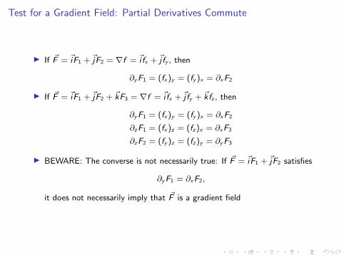
Test for a Gradient Field: Partial Derivatives Commute

I If ~F = ~iF1 + ~jF2 = ∇f = ~i fx + ~j fy , then

∂yF1 = (fx)y = (fy )x = ∂xF2

I If ~F = ~iF1 + ~jF2 + ~kF3 = ∇f = ~i fx + ~j fy + ~kfz , then

∂yF1 = (fx)y = (fy )x = ∂xF2

∂zF1 = (fx)z = (fz)x = ∂xF3

∂zF2 = (fy )z = (fz)y = ∂yF3

I BEWARE: The converse is not necessarily true: If ~F = ~iF1 + ~jF2 satisfies

∂yF1 = ∂xF2,

it does not necessarily imply that ~F is a gradient field

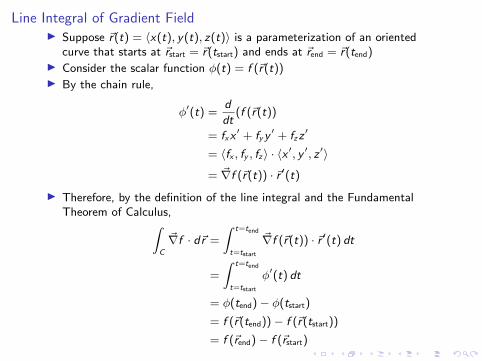
Line Integral of Gradient FieldI Suppose ~r(t) = 〈x(t), y(t), z(t)〉 is a parameterization of an oriented

curve that starts at ~rstart = ~r(tstart) and ends at ~rend = ~r(tend)I Consider the scalar function φ(t) = f (~r(t))I By the chain rule,

φ′(t) =d

dt(f (~r(t))

= fxx′ + fyy

′ + fzz′

= 〈fx , fy , fz〉 · 〈x ′, y ′, z ′〉

= ~∇f (~r(t)) · ~r ′(t)

I Therefore, by the definition of the line integral and the FundamentalTheorem of Calculus,∫

C

~∇f · d~r =

∫ t=tend

t=tstart

~∇f (~r(t)) · ~r ′(t) dt

=

∫ t=tend

t=tstart

φ′(t) dt

= φ(tend)− φ(tstart)

= f (~r(tend))− f (~r(tstart))

= f (~rend)− f (~rstart)

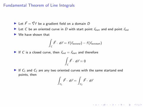
Fundamental Theorem of Line Integrals

I Let ~F = ~∇f be a gradient field on a domain D

I Let C be an oriented curve in D with start point ~rstart and end point ~rend

I We have shown that∫C

~F · d~r = f (~rtextend)− f (~rtextstart)

I If C is a closed curve, then ~rend = ~rstart and therefore∫C

~F · d~r = 0

I If C1 and C2 are any two oriented curves with the same startand endpoints, then ∫

C1

~F · d~r =

∫C2

~F · d~r

Path Independent, Conservative, Gradient Vector Fields

I A vector field ~F is path-independent on a domain D, if, for any twooriented curves C1 and C2 in D with the same start points and same endpoints, ∫

C1

~F · d~r =

∫C2

~F · d~r

I A vector field ~F is path-independent on a domain D, if, for any closedcurve C in D, ∫

C

~F · d~r = 0

I A vector field ~F is gradient or conservative on a domain D, if there is apotential function f on domain D such that ~∇f = ~F

I Any path-independent vector field on a domain D is conservative, and anyconservative vector field on a domain D is path-independent

I Gradient ⇐⇒ conservative ⇐⇒ path-independent