Dead fuel moisture estimation with MSG–SEVIRI data. Retrieval of meteorological data for the calculation of the equilibrium moisture content

This article appeared in a journal published by Elsevier. The attachedcopy is furnished to the author for internal non-commercial researchand education use, including for instruction at the authors institution

and sharing with colleagues.

Other uses, including reproduction and distribution, or selling orlicensing copies, or posting to personal, institutional or third party

websites are prohibited.

In most cases authors are permitted to post their version of thearticle (e.g. in Word or Tex form) to their personal website orinstitutional repository. Authors requiring further information

regarding Elsevier’s archiving and manuscript policies areencouraged to visit:

http://www.elsevier.com/copyright

Author's personal copy

Agricultural and Forest Meteorology 150 (2010) 861–870

Contents lists available at ScienceDirect

Agricultural and Forest Meteorology

journa l homepage: www.e lsev ier .com/ locate /agr formet

Dead fuel moisture estimation with MSG–SEVIRI data. Retrieval ofmeteorological data for the calculation of the equilibrium moisture content

Héctor Nietoa,b,∗, Inmaculada Aguadoa, Emilio Chuviecoa, Inge Sandholtb

a Department of Geography, University of Alcalá, Colegios 2, 28801, Alcalá de Henares, Spainb Department of Geography and Geology, University of Copenhagen, Øster Volgade 10, 1350, Copenhagen K, Denmark

a r t i c l e i n f o

Article history:Received 26 October 2009Received in revised form 4 February 2010Accepted 12 February 2010

Keywords:Remote sensingEquilibrium moisture contentAir temperatureRelative humidityMSG–SEVIRIThermal infraredPrecipitable water

a b s t r a c t

In this study we propose to use remote sensing data to estimate hourly meteorological data and thenassess the moisture content of dead fuels. Three different models to estimate the equilibrium moisturecontent (EMC) were applied together with remotely sensed retrieved air temperature and relative humid-ity. The input data were acquired by the Spinning Enhanced Visible and Infrared Imager (SEVIRI) sensor, onboard the Meteosat Second Generation (MSG) satellite, from which air temperature and relative humid-ity were estimated every 15 min. Air temperature estimations are based on the Temperature-VegetationIndex (TVX) algorithm. This algorithm exploits the inverse linear relationship between the land surfacetemperature and the vegetation fractional cover. This relationship was evaluated in a spatial windowwhere the meteorological forcing is assumed to be constant. To estimate the vapour pressure, a lin-ear relationship between precipitable water content and vapour pressure has been derived. Precipitablewater content was estimated with the thermal infrared bands of SEVIRI using a split-window algorithmand data from ground meteorological stations in Spain during the year 2005 were used to calibrate andvalidate the vapour pressure models. Finally air temperature and vapour pressure were combined tocalculate the EMC for dead fuels and the transfer of errors of these estimates have been assessed withground meteorological data for three different EMC models. Promising results were obtained, with meanabsolute errors ranging from 1.9% to 2.7% of moisture content depending on the applied EMC model, butthe remote sensed EMC tends to underestimate the EMC from ground data. Improvements in air temper-ature and vapour pressure estimations would lead to a better agreement between the observed and thepredicted values.

© 2010 Elsevier B.V. All rights reserved.

1. Introduction

Most fire danger assessment systems take into account the fuelmoisture content (FMC) of dead fuels, since moisture is closelyrelated to fire ignition and propagation potential (Bradshaw andDeeming, 1983). Laboratory studies have shown high correla-tions between FMC and the ignition delay (Dimitrakopoulos andPapaioannou, 2001), while many studies have identified closelinks between FMC and both fire rate of spread and fire intensity(Rothermel, 1972). In the case of surface fires, the fire front propa-gates through the forest floor and thus the moisture of dead fuelsis critical in the rate of spread (Aguado et al., 2007; Viney, 1991).

Unlike live vegetation, which can regulate water losses throughstomatal closure and water uptake by roots, moisture in dead fuelsis subject to sorption, precipitation and latent heat processes (Ruiz

∗ Corresponding author. Tel.: +45 3532 2500; fax: +45 3532 2501.E-mail addresses: [email protected] (H. Nieto), [email protected]

(I. Aguado), [email protected] (E. Chuvieco), [email protected] (I. Sandholt).

Gonzalez et al., 2009; Viney and Catchpole, 1991). Dead fuels tendto gain or lose moisture until an equilibrium with the surround-ing atmosphere is achieved. This steady moisture content is calledequilibrium moisture content (EMC) and is governed by meteoro-logical factors, fuel type, and hysteresis (Catchpole et al., 2001; RuizGonzalez et al., 2009; Viney and Catchpole, 1991). The rate at whichfuels tends to this equilibrium is governed by the rate of diffusionof moisture through the fuel and is called the response time (Vineyand Catchpole, 1991; Viney, 1991). This response time is defined asthe time taken for the fuel to achieve about the 63% (1 − 1/e) of thechange from its initial moisture content to the EMC (Catchpole etal., 2001; Viney and Catchpole, 1991), and it primarily depends onfuel size (Catchpole et al., 2001; Viney, 1991).

Temperature (T) and relative humidity (RH) are the primarymeteorological factors that affect EMC (Viney and Catchpole, 1991).Simard (1968) developed an empirical estimate of EMC based ona set of three equations that depend on the relative humidity (Eq.(1)). This model was calibrated for desorbing wood material (Viney,1991) but it has been applied to fine fuels as well, such as in thecase of the U.S. National Fire Danger Rating System (Bradshaw and

0168-1923/$ – see front matter © 2010 Elsevier B.V. All rights reserved.doi:10.1016/j.agrformet.2010.02.007

Author's personal copy

862 H. Nieto et al. / Agricultural and Forest Meteorology 150 (2010) 861–870

Deeming, 1983).

RH < 10;EMC = 0.03 + 0.2626RH − 0.00104RHT10 ≤ RH < 50;EMC = 1.76 + 0.1601RH − 0.02660T

RH ≥ 50;EMC = 21.06 − 0.4944RH + 0.005565RH2

−0.00063RHT

(1)

Another empirical model was developed along with the CanadianFire Weather Index (Van Wagner, 1987). It was originally pro-posed by Van Wagner (1972) and later modified by VanWagnerand Pickett (1985) to force the EMC converge at zero when RH tendsto zero (Viney, 1991). This model take into account the hysteresisphenomenon. The equations for desorption (EMCd) and adsorption(EMCw) processes are:

EMCd = 0.942RH0.679 + 0.000499e0.1RH

+0.18 (21.1 − T)(

1 − e−0.115RH)

(2a)

EMCw = 0.618RH0.753 + 0.000454e0.1RH

+0.18 (21.1 − T)(

1 − e−0.115RH)

(2b)

On the other hand, a semi-empirical model to estimate EMC wasproposed by Nelson (1984), who found a relationship between theEMC and the logarithmic change of the Gibbs free energy (Eq. (3)):

EMC = 100B

ln( −RT

M exp Aln

RH100

)(3)

where R is the universal gas constant, M is the molecular weightof water, and A and B are two parameters that must be evaluatedfor each fuel type and whether the involved process is desorptionor adsorption. In addition, these coefficients may also vary withtemperature.

Traditionally, these models have been applied with observeddata from meteorological ground stations or with forecast datafrom numerical weather prediction (NWP) models. Ground sta-tions provide accurate and updated observations of meteorologicalvariables. However, weather networks are sparse and many timesthe stations are primarily located in agricultural or urban areas.For these reasons, several authors have recommended using fore-cast data based on NWP to replace weather observations, sinceNWP provide spatially distributed data at a reasonable resolutionby downscaling and interpolating the surface meteorological vari-ables (Aguado et al., 2007). Apart from the uncertainty caused bythe downscaling and interpolation, it is worth noting that deal-ing with forecast data may deviate from observations due to thestochastic nature of the atmosphere. Finally, these EMC modelsserve as inputs, together with precipitation data, for drying algo-rithms in order to estimate the moisture of dead fuels (Bradshawand Deeming, 1983; Van Wagner, 1987). A method proposed byBradshaw and Deeming (1983) allows the estimation of fine deadfuels, with time lags of 1 and 10 h, by simply using the EMC com-puted at the mid afternoon observation time. In Spain, Aguado etal. (2007) showed the relationship between moisture field samplesof cured grass and litter with the 10-H timelag fuel moisture modelcomputed with Bradshaw’s equations in a six-year period.

Remote sensing can provide spatially distributed informationabout the moisture content of fuels at an adequate spatial and tem-poral resolution. Most studies to estimate fuel moisture contentwith remote sensing data have dealt with live fuels, since certainwavelengths in the optical domain are related to vegetation green-ness and leaf water content (Ceccato et al., 2002; Dennison et al.,2005; Fensholt and Sandholt, 2003; Garcia et al., 2008; Hao and Qu,2007; Yebra et al., 2008).

1.1. Air temperature estimation

Empirical approaches to estimate air temperature with thermalinfrared data can be found in Cresswell et al. (1999), Cristobal etal. (2008), Chokmani and Viau (2006), Jang et al. (2004), or Vogt etal. (1997). An interesting approach was proposed by Nemani andRunning (1989) and Goward et al. (1994). This algorithm (hereaftercalled TVX) is based on the observed inverse linear relationshipbetween the land surface temperature (LST) and a vegetation index(NDVI), as a measure of fractional vegetation cover. The NormalizedDifference Vegetation Index (NDVI, Rouse et al. (1974)) is computedfrom Eq. (4):

NDVI = �NIR − �red

�NIR + �red(4)

where �NIR and �red are the near-infrared and red reflectances,respectively.

The TVX algorithm assumes that as the vegetation coverincreases, the LST approaches the air temperature, since surfacetemperature of canopies tends to be similar to the temperature ofair. Therefore, using a linear regression between LST and NDVI ina spatial window small enough to assume a constant atmosphericforcing, the air temperature can be retrieved by extrapolating thisline to an NDVI that represents a full fractional vegetation cover(hereafter called NDVImax). For more details about this algorithmthe reader is addressed to Goward et al. (1994), Prihodko andGoward (1997), or Stisen et al. (2007).

1.2. Vapour pressure estimation

Most of the water vapour is concentrated in the lowest layers ofthe atmosphere. This decrease of water vapour through the atmo-sphere has been described by a power law (Smith, 1996). Smith(1996) proposed a logarithmic relationship between the total pre-cipitable water in the atmosphere and the dew-point temperaturein surface. This relationship is dependent on the atmospheric estate,expressed by the parameter �, which is precisely the exponent ofthe power law and describes the atmospheric moisture profile. Theauthor tabulated different values for � according to the season ofthe year and the latitude considered. However, he pointed out thatbetter agreements could be obtained by adjusting this parameterto individual stations. Several authors emphasised the importanceof the length of the observation period, with higher accuracies forlonger periods such as monthly averages (Bolsenga, 1965; Schwarz,1968; Smith, 1996). Despite of this, several authors have relatedsurface humidity to atmospheric precipitable water in a daily basiswith remote sensing data (Prince et al., 1998; Goward et al., 1994;Czajkowski et al., 2000). A good distribution of water through theatmospheric profile is required to get a reliable relation betweenthe total atmospheric water content and the surface layer (Gowardet al., 1994). Low pressure systems enhance the distribution ofmoisture, as well as incoming solar radiation during daytime, sincesurface heating favours vertical mixing (Schwarz, 1968).

1.3. Precipitable water column estimation

Precipitable water in the atmosphere (W) is the main absorberof radiation in the thermal infrared region (Kleespies and McMillin,1990), and therefore thermal remote sensing is very useful to esti-mate W. The effect of the attenuation of water vapour is differentin adjacent wavebands. This differential absorption in the ther-mal infrared is the basis for split-window algorithms that estimateW (Choudhury et al., 1995). These split-window algorithms arebased on the decrease that water vapour causes on the atmospherictransmittance in wavelengths around 12 �m compared to wave-lengths around 11 �m (Jedlovec, 1990; Kleespies and McMillin,

Author's personal copy

H. Nieto et al. / Agricultural and Forest Meteorology 150 (2010) 861–870 863

1990). For instance, Choudhury et al. (1995) found a linear rela-tionship, dependent upon the emissivities, between the brightnesstemperature difference in the split-window and W. However, thesplit window channels are also affected by both surface and airtemperatures. Suggs et al. (1998) developed a physical based split-window algorithm, but their model required a priori initial guessvalues for temperature and moisture profiles, as well as for Wand LST. To avoid the use of a priori guess values, Kleespies andMcMillin (1990) proposed the use of multiple observations underchanging surface temperature conditions. With this approach, thedependence of both land surface and air temperature is eliminated.Assuming that W keeps invariable between these two observations,the ratio of transmittance can be derived from Eq. (5).

�11

�12= TA

11 − TB11

TA12 − TB

12

(5)

where � is the atmospheric transmittance, T is the brightnesstemperature, the subscripts 11 and 12 refer to the split-windowwavelengths (in �m), and the superscripts A and B represent twodifferent observation situations.

Jedlovec (1990) applied this methodology in a contextual algo-rithm for AVHRR images, under the assumption that W is invariantwithin the scene. He found that W is related to the variations ofthe split-window brightness temperatures through a logarithmicfunction. However, the assumption of invariant atmospheric con-ditions in the scene may limit the applicability of this approachin mountainous regions, where W can change due to changesin topography (Li et al., 2003). To overcome with this limita-tion, both Schroedter-Homscheidt et al. (2008) and Sobrino andRomaguera (2008) proposed to exploit the daily cycle of tempera-ture with MSG–SEVIRI in order to retrieve the transmittance ratio.Assuming equal emissivities, a polynomial function relates W tothe brightness temperature at two times. Compared to the third-order polynomial function proposed by Schroedter-Homscheidt etal. (2008), Sobrino and Romaguera (2008) showed that a secondorder polynomial function is enough accurate. Moreover, the coeffi-cients of the polynomial function are view zenith angle dependent,and thus the final expression for retrieving the precipitable watervapour is shown in Eq. (6) (Sobrino and Romaguera, 2008).

W = aarg2 + barg + ca = −15.1 sec � + 5.1b = 16.4 sec � − 2.8c = 0.336 sec � − 0.117

arg = 1sec �

ln

(TA

11 − TB11

TA12 − TB

12

) (6)

where � is the view zenith angle. In order to avoid noisy effects,a minimum difference in brightness temperature in T12 betweenboth situations A and B is required (Schroedter-Homscheidt et al.,2008; Sobrino and Romaguera, 2008). This constraint may limitthe applicability of the algorithm in snow-covered regions and inwetlands (Schroedter-Homscheidt et al., 2008).

This study is based on the hypothesis that it is feasible to retrievedead fuel moisture content from remote sensing data through theapplication of the equilibrium moisture content approach, sincethermal remote sensing has been proven to be useful to esti-mate both surface air temperature and water vapour pressure. Theobjective of this study is therefore to estimate the equilibriummoisture content through the retrieval or air temperature and rel-ative humidity with remote sensing data. Air temperature will beestimated through the TVX algorithm whereas a model for esti-mating the vapour pressure from precipitable water retrieved withthermal infrared data will be developed. Images from MeteosatSecond Generation-Spinning Enhanced Visible and Infrared Imager(MSG–SEVIRI) were selected due to its excellent temporal reso-

lution (15 minutes) allowing a near-real time assessment of themoisture of dead fuels.

2. Data

2.1. MSG–SEVIRI images

The MSG–SEVIRI sensor provides images every 15 min at a spa-tial sampling of 3km at sub-pixel nadir in 12 spectral channels,covering both the optical and thermal spectrum (Schmetz et al.,2002). The satellite is located at 0◦ latitude and 0◦ longitude, andcovers Europe, Africa, the Middle East, and partly South America.

Visible and near infrared bands, centered at 0.6 �m and 0.8 �mwavelengths, as well as thermal images (centered at 10.8 �m and12.0 �m wavelengths) from the Iberian Peninsula (Upper left cor-ner: 44.393968◦ N, 10.894700◦ W; Lower right corner: 35.184872◦

N, 1.616629◦ E) were extracted and resampled at a spatial res-olution of 4 km for the year 2005. Images were acquired andpreprocessed by the Department of Geography and Geology at theUniversity of Copenhagen, Denmark. In addition, the EUMETSATcloud mask product was also acquired for the same study periodthrough the EUMETCAST service. This product is a simplificationof the Cloud Analysis Image product, which is based on a seriesof threshold tests to detect and characterise clouds (EUMETSAT,2007).

2.2. Meteorological data

Daily meteorological data have been obtained from twodifferent sources. The Agro-climatic Information System for Irri-gation (SIAR; Sistema de Información Agroclimática para elRegadío, http://www.mapa.es/siar/), which comprises 361 auto-matic agrometeorological weather stations; and the meteorologicalsystem of Galicia (MeteoGalicia, http://www.meteogalicia.es/),with 75 meteorological stations. Both sources have developed webapplications to easily query and download their data at no cost.

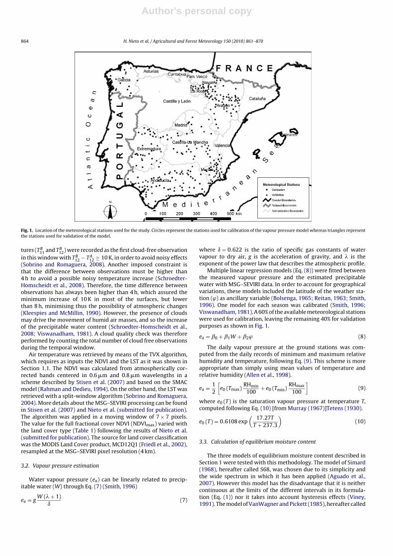
Data from 284 stations were used for this study, located inthe regions of Andalucía, Aragón, Castilla-La Mancha, Extremadura,Galicia, Murcia, Navarra, and La Rioja (Fig. 1). Most of the climaticvariability in Spain has thus been covered by this set of stations as itis shown in Fig. 1. They were selected on the basis of being furtherthan 8km (2 MSG–SEVIRI pixels) from neighbour stations or thecoast. Daily records of maximum and minimum relative humidityand temperature were extracted for the year 2005. 267 of theseground stations belong to the SIAR, and the remaining 17 belong toMeteoGalicia. In addition to these daily data, La Rioja SIAR serviceallows the download of hourly temperature and relative humidity.This hourly data has been used as well for validation purposes.

3. Methods

3.1. Satellite processing

Bands centered in 10.8 �m and 12.0 �m wavelengths for theIberian Peninsula were used together with the EUMETSAT cloudmask to produce daily estimates of W. We exploited the air temper-ature daily cycle of MSG–SEVIRI applying the algorithm proposedby Sobrino and Romaguera (2008). They proposed to apply thealgorithm in two instants, at 5:00 h and 11:00 h, and imposing thecondition of a difference in the 12.0 �m brightness temperaturebetween these two situations higher than 10 K. In order to ensuremore valid observations, we have used a different scheme in thepresent study: (1) The early morning brightness temperature issearched in a temporal window between 5:00 h and 8:45 h. Thefirst cloud-free pixel within this temporal window is registeredas TA

11 and TA12. (2) Next, the near-noon brightness temperature is

searched in a window between 9:00 h and 12:45 h. These tempera-

Author's personal copy

864 H. Nieto et al. / Agricultural and Forest Meteorology 150 (2010) 861–870

Fig. 1. Location of the meteorological stations used for the study. Circles represent the stations used for calibration of the vapour pressure model whereas triangles representthe stations used for validation of the model.

tures (TB11 and TB

12) were recorded as the first cloud-free observationin this window with TB

12 − TA12 ≥ 10 K, in order to avoid noisy effects

(Sobrino and Romaguera, 2008). Another imposed constraint isthat the difference between observations must be higher than4 h to avoid a possible noisy temperature increase (Schroedter-Homscheidt et al., 2008). Therefore, the time difference betweenobservations has always been higher than 4 h, which assured theminimum increase of 10 K in most of the surfaces, but lowerthan 8 h, minimising thus the possibility of atmospheric changes(Kleespies and McMillin, 1990). However, the presence of cloudsmay drive the movement of humid air masses, and so the increaseof the precipitable water content (Schroedter-Homscheidt et al.,2008; Viswanadham, 1981). A cloud quality check was thereforeperformed by counting the total number of cloud free observationsduring the temporal window.

Air temperature was retrieved by means of the TVX algorithm,which requires as inputs the NDVI and the LST as it was shown inSection 1.1. The NDVI was calculated from atmospherically cor-rected bands centered in 0.6 �m and 0.8 �m wavelengths in ascheme described by Stisen et al. (2007) and based on the SMACmodel (Rahman and Dedieu, 1994). On the other hand, the LST wasretrieved with a split-window algorithm (Sobrino and Romaguera,2004). More details about the MSG–SEVIRI processing can be foundin Stisen et al. (2007) and Nieto et al. (submitted for publication).The algorithm was applied in a moving window of 7 × 7 pixels.The value for the full fractional cover NDVI (NDVImax) varied withthe land cover type (Table 1) following the results of Nieto et al.(submitted for publication). The source for land cover classificationwas the MODIS Land Cover product, MCD12Q1 (Friedl et al., 2002),resampled at the MSG–SEVIRI pixel resolution (4 km).

3.2. Vapour pressure estimation

Water vapour pressure (ea) can be linearly related to precip-itable water (W) through Eq. (7) (Smith, 1996)

ea = gW (� + 1)

ı(7)

where ı = 0.622 is the ratio of specific gas constants of watervapour to dry air, g is the acceleration of gravity, and � is theexponent of the power law that describes the atmospheric profile.

Multiple linear regression models (Eq. (8)) were fitted betweenthe measured vapour pressure and the estimated precipitablewater with MSG–SEVIRI data. In order to account for geographicalvariations, these models included the latitude of the weather sta-tion (ϕ) as ancillary variable (Bolsenga, 1965; Reitan, 1963; Smith,1996). One model for each season was calibrated (Smith, 1996;Viswanadham, 1981). A 60% of the available meteorological stationswere used for calibration, leaving the remaining 40% for validationpurposes as shown in Fig. 1.

ea = ˇ0 + ˇ1W + ˇ2ϕ (8)

The daily vapour pressure at the ground stations was com-puted from the daily records of minimum and maximum relativehumidity and temperature, following Eq. (9). This scheme is moreappropriate than simply using mean values of temperature andrelative humidity (Allen et al., 1998).

ea = 12

[e0 (Tmax)

RHmin

100+ e0 (Tmin)

RHmax

100

](9)

where e0 (T) is the saturation vapour pressure at temperature T,computed following Eq. (10) [from Murray (1967)]Tetens (1930).

e0 (T) = 0.6108 exp(

17.27T

T + 237.3

)(10)

3.3. Calculation of equilibrium moisture content

The three models of equilibrium moisture content described inSection 1 were tested with this methodology. The model of Simard(1968), hereafter called S68, was chosen due to its simplicity andthe wide spectrum in which it has been applied (Aguado et al.,2007). However this model has the disadvantage that it is neithercontinuous at the limits of the different intervals in its formula-tion (Eq. (1)) nor it takes into account hysteresis effects (Viney,1991). The model of VanWagner and Pickett (1985), hereafter called

Author's personal copy

H. Nieto et al. / Agricultural and Forest Meteorology 150 (2010) 861–870 865

Table 1Calibrated TVX-NDVImax values corresponding to each of the IGBP biomes in theIberian Peninsula.

Code IGBP class NDVImax

1 Evergreen needleleaved forest 0.8492 Evergreen broadleaved forest 0.9344 Deciduous broadleaved forest 1.1625 Mixed forests 0.9956 Closed shrublands 0.9157 Open shrublands 0.8038 Woody savannas 0.8359 Savannas 0.777

10 Grasslands 0.98512 Croplands 0.80013 Urban and built-up 0.78014 Cropland/Natural vegetation mosaic 0.937

Source: Nieto et al. (submitted for publication).

vW85, was chosen because it has also been widely applied and itis continuous in the whole range of data. Uniquely the formulationcorresponding to the desorption process (Eq. (2a)) was taken intoaccount to be comparable with the S68 model. Finally, the semi-empirical approach of Nelson (1984), hereafter called N84, wasalso compared. The values for coefficients A and B in Eq. (3) werethose proposed by Nelson (1984) for Pinus ponderosa in a desorptionprocess at a temperature of 25 ◦C.

To adjust the atmospheric relative humidity and temperature atthe fuel-atmosphere interface, the factors shown in Table 2 wereused as they were proposed by Bradshaw and Deeming (1983). Thistable requires as ancillary variable the sky condition. Therefore, adaily sky condition was computed, in a pixel basis, as the propor-tion cloud MSG–SEVIRI observations to the total of observationsbetween 8:00 h and 16:00 h. For this purpose the standard SEVIRIcloud mask product was used (EUMETSAT, 2007).

15 min relative humidity (RH) was computed with observationsbetween 8:00 h and 16:00 h, since it is the time window with avail-able air temperature estimations (Eq. (11)).

RH(%) = 100ea

e0(11)

The saturation vapour pressure has been computed with Eq. (10)by substituting the retrieved 15 min TVX temperature into T.

3.4. Validation

Vapour pressure was assessed with daily data from the agrom-eteorological stations that have not been used for calibration (40%of the dataset, Fig. 1). On the other hand, the hourly maximumtemperature and the minimum relative humidity estimates werevalidated with the hourly data from the ground stations in La Riojathat were not used in the calibration process. Finally, the transferof errors from these estimates to the EMC models were assessed aswell with data from La Rioja ground stations.

The bias, the mean absolute error (MAE), and the root meansquare error (RMSE) were computed as error measurements(Willmott, 1982; Willmott and Matsuura, 2005). The slope b andthe intercept a of the regression between the observed versusthe predicted (Pineiro et al., 2008) as well as the Pearson corre-

Table 3Seasonal and annual descriptive statistics for � parameter. � values below 0 havebeen discarded for the analyses.

Season N Min Mean Max S.D.

Winter 9849 0.01 2.67 47.46 2.71Spring 13373 0.02 2.64 46.26 2.95Summer 17112 0.12 2.77 102.82 2.21Autumn 8731 0.07 3.43 90.99 3.51Year 49065 0.01 2.83 102.82 2.57

lation coefficient r were computed as agreement measures. Finally,in order to allow an accuracy comparison between the differentestimates (meteorological variables and modelled EMCs), Theil’sdecomposition of errors was performed (Smith and Rose, 1995).Theil’s coefficients (Eq. (12)) partition the sum of the squared errorsbetween the observed and the predicted in a proportion associatedwith (1) mean differences between the observed and predictedvalues, Ubias; (2) deviations from the 1:1 line, Uslope; and (3) theunexplained variance, Uerror.

Ubias =N(

O − P)2∑

(O − P)2

Uslope =(b − 1)2 ∑(

P − P)2∑

(O − P)2

Uerror =∑(

O − O)2∑

(O − P)2

(12)

where N is the number of elements, O and P are the observed andpredicted values, respectively; O and P are the observed and pre-dicted mean, respectively; and O = a + bP. Since the coefficientsrepresent a proportion of the total error, the sum of the three coef-ficients is 1. A good model should neither deviate from the 1:1 linenor have a bias. Therefore Ubias and Uslope should be close to zerowhereas Uerror should be close to unity.

4. Results

A total of 59,507 valid estimations of W located over the groundstations were obtained during the year 2005. However, cases with alow precipitable water (W < 0.1 cm) were suppressed in followinganalyses in order to avoid noisy effects caused by the sensor sig-nal in very dry atmospheres (Kleespies and McMillin, 1990). Thisfilter left 59,281 cases. When crossing the retrieved W with the cal-culated vapour pressure at the ground stations, a total of 49,166cases were obtained. The � parameter, which describes the atmo-sphere profile, was then computed by reordering Eq. (7). Assumingthat moisture decreases through the atmosphere with the altitude,this parameter must be positive. Therefore, all cases with negativevalues of � were discarded for future analysis. Table 3 shows thedescriptive statistics of this parameter. The annual mean is 2.83,being the mean values higher in autumn and summer (3.43 and2.77, respectively) than during spring and winter (2.64 and 2.67,respectively).

Once these filters were applied, 29,651 cases were used to cali-brate the daily vapour pressure estimation, leaving other 19,414cases to validate the model. One model was calibrated per sea-

Table 2Fuel temperature and relative humidity adjustment factors adapted from Bradshaw and Deeming (1983). The sky condition is computed as the proportion of MSG–SEVIRIcloud detections between 8:00 h and 16:00 h.

Sky condition

Clear (0–0.1) Scattered (0.1–0.5) Broken (0.5–0.9) Overcast (0.9–1)

T add (celsius) 13.9 10.6 6.7 2.8RH multiply 0.75 0.83 0.91 1

Author's personal copy

866 H. Nieto et al. / Agricultural and Forest Meteorology 150 (2010) 861–870

Table 4Multiple linear regression between water vapour pressure and precipitable water(W) and Latitude.

Season N R2 Intercept W (cm) Latitude (◦)

Winter 5935 0.29 * 1.00 * 0.20 * −0.017 *

Spring 8081 0.30 * 0.58 * 0.22 * −0.001Summer 10363 0.32 * 1.28 * 0.26 * −0.017 *

Autumn 5272 0.30 * 1.21 * 0.22 * −0.019 *

Year 29651 0.47 * 0.83 * 0.32 * −0.012 *

* Significant coefficients (p < 0.01) were flagged with an asterisk.

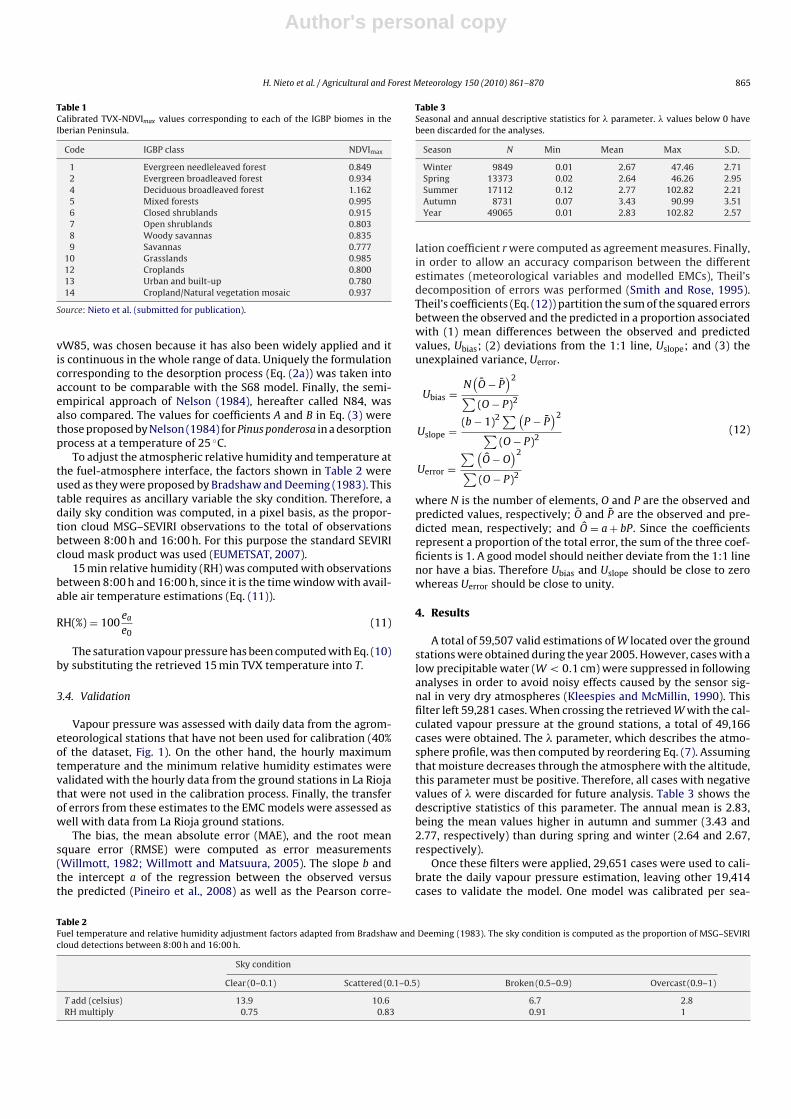
son during the year 2005. The results are shown in Table 4. Thevalidation of the vapour pressure (Table 5) showed no signifi-cant bias (0.002 kPa, Ubias = 0.00) and an accuracy of 0.182 kPa interms of MAE. In addition, the slope was very close to 1 (b = 1.030,Uslope = 0.00, see Fig. 2a). Therefore, the error contribution in themodel may be assigned completely to the unexplained variance(Uerror = 1), with a Pearson correlation coefficient of 0.77.

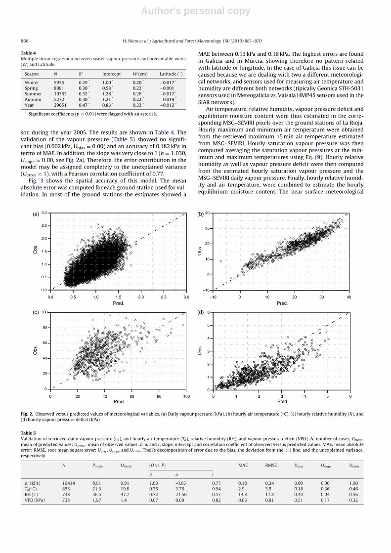
Fig. 3 shows the spatial accuracy of this model. The meanabsolute error was computed for each ground station used for val-idation. In most of the ground stations the estimates showed a

MAE between 0.13 kPa and 0.18 kPa. The highest errors are foundin Galicia and in Murcia, showing therefore no pattern relatedwith latitude or longitude. In the case of Galicia this issue can becaused because we are dealing with two a different meteorologi-cal networks, and sensors used for measuring air temperature andhumidity are different both networks (tipically Geonica STH-5031sensors used in Meteogalicia vs. Vaisala HMP45 sensors used in theSIAR network).

Air temperature, relative humidity, vapour pressure deficit andequilibrium moisture content were thus estimated in the corre-sponding MSG–SEVIRI pixels over the ground stations of La Rioja.Hourly maximum and minimum air temperature were obtainedfrom the retrieved maximum 15 min air temperature estimatedfrom MSG–SEVIRI. Hourly saturation vapour pressure was thencomputed averaging the saturation vapour pressures at the min-imum and maximum temperatures using Eq. (9). Hourly relativehumidity as well as vapour pressure deficit were then computedfrom the estimated hourly saturation vapour pressure and theMSG–SEVIRI daily vapour pressure. Finally, hourly relative humid-ity and air temperature, were combined to estimate the hourlyequilibrium moisture content. The near surface meteorological

Fig. 2. Observed versus predicted values of meteorological variables. (a) Daily vapour pressure (kPa), (b) hourly air temperature (◦C), (c) hourly relative humidity (%), and(d) hourly vapour pressure deficit (kPa)

Table 5Validation of retrieved daily vapour pressure (ea), and hourly air temperature (Ta), relative humidity (RH), and vapour pressure deficit (VPD). N, number of cases; Pmean,mean of predicted values; Omean, mean of observed values; b, a, and r, slope, intercept and correlation coefficient of observed versus predicted values. MAE, mean absoluteerror; RMSE, root mean square error; Ubias, Uslope and Uerror, Theil’s decomposition of error due to the bias, the deviation from the 1:1 line, and the unexplained variance,respectively.

N Pmean Omean (O vs. P) MAE RMSE Ubias Uslope Uerror

b a r

ea (kPa) 19414 0.91 0.91 1.03 -0.03 0.77 0.18 0.24 0.00 0.00 1.00Ta(◦C) 853 21.3 19.8 0.75 3.76 0.94 2.9 3.5 0.18 0.36 0.46RH (%) 738 36.5 47.7 0.72 21.56 0.57 14.8 17.8 0.40 0.04 0.56VPD (kPa) 738 1.97 1.4 0.67 0.08 0.82 0.66 0.81 0.51 0.17 0.32

Author's personal copy

H. Nieto et al. / Agricultural and Forest Meteorology 150 (2010) 861–870 867

Fig. 3. Spatial distribution of the vapour pressure mean absolute error (MAE). Only ground stations used for validation have been represented. The values were binnedfollowing a geometric series

estimates were scaled to the temperature and relative humidityat the fuel-atmosphere interface, according to Table 2, using thesky condition variable computed through the MSG–SEVIRI cloudmask data (EUMETSAT, 2007).

Table 5 shows the validation assessment of the meteorologi-cal MSG–SEVIRI estimates with the hourly ground measurementsin La Rioja stations. Air temperature shows a MAE of 2.9 ◦ C anda RMSE of 3.5 ◦C, with a mean bias of 1.5 ◦C. The bias is respon-sible of 18% of the total error, whereas the lack of unity slope(b = 0.75) and the unexplained variance represents the 36% and46% of the error, respectively. Fig. 2(b) shows the scatterplot ofobserved versus predicted. This figure shows that the model tendsto underprediction at low temperatures and to overprediction athigh temperatures.

Both relative humidity (RH) and vapour pressure deficit (VPD)show similar patterns, with an underestimation of humidity (meanbias of −12.2% and 0.564 kPa respectively for RH and VPD). RHshowed a MAE = 14.7% and RMSE = 17.8%, whereas VPD had anMAE = 0.663 kPa and an RMSE = 0.806 kPa. Most of the error inestimating RH comes from the unexplained variance by the model(Uerror = 56%), followed by the bias (Ubias = 40%). As it can be seenin Fig. 2(c) and (d), the estimated RH shows a poorer performancein explaining the observed variance compared to the VPD (Pearsoncorrelation coefficient of 0.57 versus 0.82).

Three models of EMC were computed from the retrieved hourlydata after applying the correction factors to temperature and rela-tive humidity of Table 2. The three models tend to underestimate,with mean bias of −1.48%, −2.09% and −1.41%, respectively for theS68, vW85 and N84 models (Table 6 and Fig. 4). N84 showed thelowest MAE, with a value of 1.86%, which represents 19.5% of to theobserved mean (Omean = 9.52%). On the other hand, S68 and vW85showed MAEs of 1.93% and 2.73% respectively, representing the28.2% and 31.3% of the observed means (6.85% and 8.73%, respec-tively). The three models have a similar slope of the regression ofthe observed versus predicted values (b values ranging between0.78 and 0.79), but the vW85 model explained the highest vari-ance of the three models (Pearson correlation coefficient of 0.71compared to 0.62 and 0.61 for S68 and N84, respectively). In thethree models, near a 60% of the error is due to the unexplainedvariance, whereas the proportion of the error associated to the biasis close to the 40%. The contribution to the errors by the lack of slope

unity is almost insignificant for all three models (4% in the worstcase).

5. Discussion

The proposed methodology aimed to estimate the equilibriummoisture content of dead fuels in a sequential manner. First relatingthe remotely sensed atmospheric precipitable water to the vapourpressure in surface; secondly, with the estimation of the air tem-perature by means of the TVX algorithm; thirdly, the 15 minuteair temperature and the daily vapour pressure were combined toobtain the relative humidity every 15 min; and finally, by calcu-lating the EMC with the estimated air temperature and relativehumidity. Each one of these tasks is subject to error. The sourceof possible errors for each task as well as the transfer of errors inEMC models will be discussed in the following paragraphs.

5.1. Vapour pressure

The vapour pressure is related to the atmospheric precipitablewater through the � parameter. In this study, � values for eachseason ranged between 2.6 and 3.4 (Table 3), having the same orderthat the originally proposed values by Smith (1996). Indeed, thosetabulated values ranged from 2.7 to 3.1 in latitudes between 30◦ and50◦. The values obtained in our study are however based on only oneyear and in a specific location compared to the values from Smith(1996), who used a more global and a longer timeseries datasetto tabulate the values of �. Descriptive statistics in Table 3 show aswell that the highest variability in atmospheric conditions is shownin spring and in autumn, with the highest standard deviation in�. The other extreme is summer, with a low standard deviationshowing that the daily atmospheric profile becomes more stableamongst days.

The linear regressions between the vapour pressure and theprecipitable water showed low coefficients of determination R2

(Table 4). This was however expected since several authors alreadypointed out the highly variability of the atmospheric profile in ahourly to daily basis (Bolsenga, 1965; Reitan, 1963; Schwarz, 1968;Smith, 1996). An estimation of decadal or monthly averages ofvapour pressure would lead to an increase of the explained vari-ance by the proposed model, and therefore it should be expected

Author's personal copy

868 H. Nieto et al. / Agricultural and Forest Meteorology 150 (2010) 861–870

Table 6Assessment of the transfer of errors for both the hourly fuel-atmosphere interface temperature (Tf ) and relative humidity (RHf ), as well as the equilibrium moisture content(EMC) models of Simard (1968), VanWagner and Pickett (1985), and Nelson (1984). N, number of cases; Pmean, mean of MSG–SEVIRI estimated values; Omean, mean of groundestimated values; b, a, and r, slope, intercept and correlation coefficient of ground versus MSG–SEVIRI estimates. MAE, mean absolute error; RMSE, root mean square error;Ubias, Uslope and Uerror, Theil’s decomposition of error due to the bias, the deviation from the 1:1 line, and the unexplained variance, respectively.

N Pmean Omean (O vs. P) MAE RMSE Ubias Uslope Uerror

b a r

Tf (◦ C) 738 35.7 33.8 0.78 5.83 0.92 2.9 3.4 0.32 0.21 0.47RHf (%) 738 28.5 37.4 0.78 15.27 0.59 11.6 14.2 0.40 0.02 0.58EMC S68 (%) 738 5.37 6.85 0.78 2.66 0.62 1.93 2.35 0.40 0.03 0.57EMC vW85 (%) 738 6.63 8.73 0.79 3.49 0.71 2.73 3.29 0.41 0.04 0.55EMC N84 (%) 738 8.11 9.52 0.78 3.20 0.61 1.86 2.26 0.39 0.03 0.58

Fig. 4. Ground versus MSG–SEVIRI estimates of equilibrium moisture content (%).(a) Simard (1968), (b) VanWagner and Pickett (1985), and (c) Nelson (1984) models

higher R2 values. However, the validation of this model showed itsfeasibility, showing no bias and a regression slope of observed ver-sus predicted very close to 1 (b = 1.03). Therefore, all of the errorsin vapour pressure estimation (MAE = 0.182 kPa) were caused bythe unexplained variance of the model (Uerror = 1.00). The uncer-tainty in the retrieval of vapour pressure increased with errorsof vapour pressure measurements, such as sensor noise or fail-ure in the assumption of daily constant vapour pressure, as well aswith errors in the MSG–SEVIRI precipitable water algorithm, whichhad an expected accuracy around 0.5 cm (Sobrino and Romaguera,2008). A reduction of these errors should improve the vapour pres-sure estimates and thus an additional increase of the explainedvariance by the model.

From Table 4 and Eq. (8), it is evident that vapour pressuredecreases with latitude, when precipitable water is constant. Thistrend can be observed as well with the tabulated values of Smith(1996), where � tends to decrease with higher latitudes. In addition,the effect of latitude seems to be constant through the year, withvalues of ˇ coefficient between −0.17 and −0.19 with the excep-tion of spring, which had a very low and not significant coefficient(p = 0.39). The moisture atmospheric profile in the Iberian Penin-sula during spring seems therefore invariant with latitude, at leastduring the year 2005. Further research should address this issue,trying to expand the dataset of observations with additional years.

5.2. Air temperature

Estimated air temperature showed good accuracy (MAE = 2.9◦ Cand RMSE = 3.5◦ C) with the observed hourly maximum temper-ature in the validation sites of La Rioja. This result improves theestimates from Nieto et al. (submitted for publication) of 5◦ C inRMSE in Spain. The improvement in the current study can be causedby the fact that the authors in the original study used to calibrateand validate interpolated daily maximum air temperature insteadof measured air temperature in ground stations.

5.3. Relative humidity

Humidity has been computed in terms of vapour pressure deficitas well as relative humidity. Similar results in VPD accuracy, havebeen found in Goward et al. (1994), with an RMSE of 0.7 kPa versusan RMSE = 0.8 kPa obtained in our study, but both studies improvesthe results obtained by Prince et al. (1998), with an RMSE = 1.1 kPa.In our study and in Goward et al. (1994) the surface humidity waslocally calibrated with ground data, whereas Prince et al. (1998)directly applied the tabulated values of � shown in Smith (1996). AsSmith (1996) pointed out in his paper, better relationships betweenthe precipitable water and surface humidity are expected to beobtained from fittings with individual stations. The modelled rela-tive humidity explained less variance compared to VPD (Table 5).Besides, Fig. 2c shows that the disagreement between the observedand the predicted values of RH is higher with increasing RH. Indeed,

Author's personal copy

H. Nieto et al. / Agricultural and Forest Meteorology 150 (2010) 861–870 869

Fig. 5. Temporal evolution of VanWagner and Pickett (1985) equilibrium moisturecontent. Dashed timeseries represents the EMC calculated with data from the stationin Santo Domingo de la Calzada (La Rioja, 42.1433◦ N, 2.9423◦ W). Plain timeseriesrepresent the EMC calculated with MSG–SEVIRI meteorological proxies for the samelocation.

by computing the derivatives of RH and VPD with air Temperature(Eqs. (13) and (14)), it can be seen that RH is more sensitive to Tvariations (namely inaccuracies) than VPD. In addition VPD varia-tions with temperature are insensitive to vapour pressure. It is thusexpected that the accuracy in estimating RH will be lower with lowtemperatures. On the contrary, low temperatures will increase theaccuracy of VPD estimations. However, these inaccuracies in RH arereduced at higher air temperatures, when the highest fire dangeris expected to occur.

dRHdT

= −4098ea

e0(T + 237.3)2

dRHdea

= 1e0

(13)

dVPDdT

= 4098e0

(T + 237.3)2

dVPDdea

= −1 (14)

In our study, vapour pressure estimates showed neither biasnor deviations from the 1:1 line, and thus it can be inferred thatmost of the inaccuracies in bias and deviations from the 1:1 linein relative humidity are caused by the air temperature estimates.On the other hand, errors caused by the unexplained variance inhumidity are mostly owing to the estimates of vapour pressure. Itis clear that improvements in the retrieval of precipitable water,vapour pressure, and especially in air temperature, will improvethe estimates of VPD and RH (Czajkowski et al., 2000; Prince et al.,1998). Finally, noise removal caused by cloud contaminated pixelsbecomes crucial in precipitable water (Jedlovec, 1990; Schroedter-Homscheidt et al., 2008; Suggs et al., 1998) and in air temperature(Czajkowski et al., 2000; Prince et al., 1998) estimations.

5.4. Equilibrium moisture content

Temperature and relative humidity at the fuel-atmosphereinterface showed the same pattern as the air measurements, with atrend to overestimate in temperature and to underestimate in rel-ative humidity. This trend causes the systematic underestimationof the equilibrium moisture content. As an example of this under-estimation in EMC, Fig. 5 shows the trend of EMC with MSG–SEVIRIdata and with ground data for the station of Santo Domingo de laCalzada (La Rioja). Al thought the EMC from MSG–SEVIRI system-atically underestimates the EMC computed with meteorologicalground data, both timeseries show the same trend.

Although the slope of the EMC models between the valuescalculated with ground measurements and those estimated withMSG–SEVIRI is around 0.78, the error contribution caused by theslope is almost negligible (Uslope ≈ 4% in the three models). Nev-

Table 7Pearson correlation coefficient between the absolute residuals of retrieved param-eters and the observed meteorological values.

Observed values Absolute residual

Tf RHf Tf RHf

Absolute Residual EMC S68 −0.24 0.63 0.42 0.99EMC vW85 −0.11 0.53 0.53 0.98EMC N84 −0.23 0.63 0.42 1.00

ertheless, deviations from the 1:1 line are almost caused by afew cases with the highest EMC values. Indeed, below a certainMSG–SEVIRI EMC value, the slope between the observed and thepredicted is not significantly (p < 0.01) different for 1. This valueis approximately 7.5% for S68 (678 out of 738 cases are below thatvalue), 10% for vW85 (641 cases), and 115 for N84 (697 cases).

EMC models are more sensitive to changes in relative humiditythan to changes in temperature (Ruiz Gonzalez et al., 2009), andtherefore the accuracy of EMC is very dependent on the accuracy inthe RH retrieval. This issue can be empirically observed in Table 7,where the Pearson correlation coefficient is shown between theresiduals of the retrieved EMC and the one calculated from groundmeteorological values. The residuals of the EMC models increasewith increasing relative humidity and decreasing temperature andthis relationship is stronger with the humidity than with the tem-perature. Finally, the magnitude of the error in EMC is completelydependent on the errors in relative humidity (r ≈ 1) between theresiduals of EMC and residuals of RH. An appropriate estimate ofrelative humidity is therefore the critical factor in the retrieval ofEMC with remote sensing data.

6. Conclusion

A methodology to estimate the equilibrium moisture contentof dead fuel with MSG–SEVIRI images have been proposed in thisstudy. Air temperature was estimated every 15 min by combin-ing the NDVI and land surface temperature from SEVIRI usingthe TVX approach (Goward et al., 1994). On the other hand, dailyvapour pressure was estimated by relating the daily precipitablewater, retrieved with a split-window algorithm developed forMSG–SEVIRI (Sobrino and Romaguera, 2008), to the surface vapourpressure calculated with data from meteorological stations. Themodelled vapour pressure showed good accuracy with no biasand no deviations from the slope unity between the observed andpredicted. On the other hand, estimates of air temperature devi-ate from the 1:1 line and show a positive bias. Vapour pressureand air temperature were then combined to estimate the relativehumidity. Since estimated air temperature tends to overpredict,the retrieved relative humidity tends to be underestimated. Finally,when these estimates of air temperature and relative humidityare combined to calculate the EMC, the results logically showeda negative bias compared to EMC calculated with surface meteo-rological data. It is crucial therefore to obtain unbiased estimatesof air temperature to avoid this underprediction on EMC. Furtherresearch should address to get better estimates of air temperature.This task could be achieved by obtaining better radiometric cor-rections for the atmospheric and bidirectional effects in NDVI. Inaddition, the algorithm developed in Nieto et al. (submitted forpublication) for estimating the NDVImax aimed the minimisationof residuals in the air temperature estimates, although these esti-mates may be biased from ground data. Therefore, an alternativemethod for the estimation of NDVImax that produces unbiased esti-mates of air temperature would be addressed in future research.Finally, an improvement in the estimation of precipitable waterbecomes as well important since it affects the retrieval of LST andthe vapour pressure estimation.

Author's personal copy

870 H. Nieto et al. / Agricultural and Forest Meteorology 150 (2010) 861–870

Acknowledgements

Part of this research has been done during a visiting stay at theDepartment of Geography and Geology at the University of Copen-hagen (Denmark). The first author has been funded by the SpanishMinistry of Science through the FPI scholarship BES-2005-7801.Special thanks to Flemming Andersen and Simon Stisen from theUniversity of Copenhagen for providing the MSG atmosphericallycorrected images. Also thanks to the Spanish Ministry of Agricul-ture, Food and Fisheries, the regional centres of the Agro-climaticInformation System for Irrigation, and Meteogalicia for providingthe meteorological database.

References

Aguado, I., Chuvieco, E., Boren, R., Nieto, H., 2007. Estimation of dead fuel moisturecontent from meteorological data in Mediter ranean areas, applications in firedanger assessment. International Journal of Wildland Fire 16, 390–397.

Allen, R., Pereira, L., Raes, D., Smith, M., 1998. Crop evapotranspiration: guidelinesfor computing crop water requirements. FAO Irrigation and Drainage Papers 56.Food and Agriculture Organization.

Bolsenga, S.J., 1965. The relationship between total atmospheric water vapor andsurface dew point on a mean daily and hourly basis. Journal of Applied Meteo-rology 4, 430–432.

Bradshaw, B.S., Deeming, J.E., 1983. The 1978 National Fire Dan ger Rating System.Technical documentation. Technical Report. USDA, Forest Service. Ogden, Utah.

Catchpole, E.A., Catchpole, W.R., Viney, N.R., McCaw, W.L., Marsden-Smedley, J.B.,2001. Estimating fuel response time and predicting fuel moisture content fromfield data. International Journal of Wildland Fire 10, 215–222.

Ceccato, P., Gobron, N., Flasse, S., Pinty, B., Tarantola, S., 2002. Designing a spectralindex to estimate vegetation water content from remote sensing data: Part 1theoretical approach. Remote Sensing of Environment 82, 188–197.

Chokmani, K., Viau, A.A., 2006. Estimation of the air temperature and the vapourquantity in atmospheric water with the help of the AVHRR data of the NOAA.Canadian Journal of Remote Sensing 32, 1–14.

Choudhury, B.J., Dorman, T.J., Hsu, A.Y., 1995. Modeled and observed relationsbetween the AVHRR split window temperature difference and atmospheric pre-cipitable water over land surfaces. Remote Sensing of Environment 51, 281–290.

Cresswell, M.P., Morse, A.P., Thomson, M.C., Connor, S.J., 1999. Estimating surface airtemperatures from Meteosat land surface temperatures using an empirical solarzenith angle model. Inter national Journal of Remote Sensing 20, 1125–1132.

Cristobal, J., Ninyerola, M., Pons, X., 2008. Modeling air temperature through acombination of remote sensing and GIS data. Journal of Geophysical ResearchAtmospheres 113. D13106, doi:10.1029/2007JD009318.

Czajkowski, K.P., Goward, S.N., Stadler, S.J., Walz, A., 2000. Ther mal remote sensing ofnear surface environmental variables: application over the Oklahoma Mesonet.Professional Geographer 52, 345–357.

Dennison, P.E., Roberts, D.A., Peterson, S.H., Rechel, J., 2005. Use of normalized dif-ference water index for monitoring live fuel moisture. International Journal ofRemote Sensing 26, 1035–1042.

Dimitrakopoulos, A., Papaioannou, K.K., 2001. Flammability assessment of Mediter-ranean forest fuels. Fire Technology 37, 143–152.

EUMETSAT, 2007. Cloud Detection for MSG – Algorithm Theoretical Basis Document.Technical Report EUM/MET/REP/07/0132. EUMETSAT. Darmstadt, Germany.

Fensholt, R., Sandholt, I., 2003. Derivation of a shortwave infrared water stress indexfrom MODIS near- and shortwave infrared data in a semiarid environment.Remote Sensing of Environment 87, 111–121.

Friedl, M.A., McIver, D.K., Hodges, J.C.F., Zhang, X.Y., Muchoney, D., Strahler, A.H.,Woodcock, C.E., Gopal, S., Schneider, A., Cooper, A., Baccini, A., Gao, F., Schaaf,C., 2002. Global land cover mapping from MODIS: algorithms and early results.Remote Sensing of Environment 83, 287–302.

Garcia, M., Chuvieco, E., Nieto, H., Aguado, I., 2008. Combining AVHRR and mete-orological data for estimating live fuel moisture content. Remote Sensing ofEnvironment 112, 3618–3627.

Goward, S.N., Waring, R.H., Dye, D.G., Yang, J.L., 1994. Ecological remote-sensing atOTTER: satellite macroscale observations. Ecological Applications 4, 322–343.

Hao, X., Qu, J.J., 2007. Retrieval of real-time live fuel moisture content using MODISmeasurements. Remote Sensing of Environment 108, 130–137.

Jang, J.D., Viau, A.A., Anctil, F., 2004. Neural network estimation of air temperaturesfrom AVHRR data. International Journal of Remote Sensing 25, 4541–4554.

Jedlovec, G.J., 1990. Precipitable water estimation from high resolution split windowradiance measurements. Journal of Applied Meteorology 29, 863–877.

Kleespies, T.J., McMillin, L.M., 1990. Retrieval of precipitable water from observa-tions in the split window over varying surface temperatures. Journal of AppliedMeteorology 29, 851–862.

Li, Z.L., Jia, L., Su, Z.B., Wan, Z.M., Zhang, R.H., 2003. A new approach for retriev-ing precipitable water from ATSR2 split-window channel data over land area.International Journal of Remote Sensing 24, 5095–5117.

Murray, F.W., 1967. On the computation of saturation vapor pressure. Journal ofApplied Meteorology 6, 203–204.

Nelson, R.M., 1984. A method for describing equilibrium moisture content of for-est fuels. Canadian Journal of Forest Research-Revue Canadienne De RechercheForestiere 14, 597–600.

Nemani, R.R., Running, J.W., 1989. Estimation of regional surface resistance toevapotranspiration from NDVI and thermal-IRAVHRR data. Journal of AppliedMeteorology 28, 276–284.

Nieto, H., Sandholt, I., Aguado, I., Chuvieco, E., Stisen, S. Air temperature estimationwith MSG–SEVIRI data: calibration and validation of the TVX algorithm for theIberian Peninsula. Remote Sensing of Environment, submitted for publication.

Pineiro, G., Perelman, S., Guerschman, J.P., Paruelo, J.M., 2008. How to evaluate mod-els: observed vs. predicted or predicted vs. observed? Ecological Modelling 216,316–322.

Prihodko, L., Goward, S.N., 1997. Estimation of air temperature from remotely sensedsurface observations. Remote Sensing of Environment 60, 335–346.

Prince, S.D., Goetz, S.J., Dubayah, R.O., Czajkowski, K.P., Thawley, M., 1998. Infer-ence of surface and air temperature, atmospheric precipitable water and vaporpressure deficit using advanced very high-resolution radiometer satellite obser-vations: comparison with field observations. Journal of Hydrology 213, 230–249.

Rahman, H., Dedieu, G., 1994. SMAC—a simplified method for the atmospheric cor-rection of satellite measurements in the solar spectrum. International Journal ofRemote Sensing 15, 123–143.

Reitan, C.H., 1963. Surface dew point and water vapor aloft. Journal of AppliedMeteorology 2, 776–779.

Rothermel, R.C., 1972. A Mathematical Model for Predicting Fire Spread in WildlandFuels. Technical Report. USDA, Forest Service. Ogden, Utah.

Rouse, J.W., Haas, R.W., Schell, J.A., Deering, D.H., Harlan, J.C., 1974. Monitoring thevernal advancement and retrogradation (Greenwave effect) of natural vegeta-tion. Type II Report for the Period April 1973 – September 1973. Goddard SpaceFlight Center. Greenbelt, MD. USA.

Ruiz Gonzalez, A.D., Vega Hidalgo, J.A., Alvarez Gonzalez, J.G., 2009. Construction ofempirical models for predicting Pinus sp. dead fine fuel moisture in NW Spain. I:response to changes in temperature and relative humidity. International Journalof Wildland Fire 18, 71–83.

Schmetz, J., Pili, P., Tjemkes, S., Just, D., Kerkmann, J., Rota, S., Ratier, A., 2002. Anintroduction to Meteosat Second Generation (MSG). Bulletin of the AmericanMeteorological Society 83, 977–992.

Schroedter-Homscheidt, M., Drews, A., Heise, S., 2008. Total water vapor col-umn retrieval from MSG–SEVIRI split window measurements exploiting thedaily cycle of land surface temperatures. Remote Sensing of Environment 112,249–258.

Schwarz, F.K., 1968. Comments on note on the relationship between total precip-itable water and surface dew point. Journal of Applied Meteorology 7, 509–510.

Simard, A., 1968. The moisture content of forest fuels—a review of the basic concepts.Technical Report. USDA, Forest Service. Ottawa, Ontario.

Smith, E.P., Rose, K.A., 1995. Model goodness-of-fit analysis using regression andrelated techniques. Ecological Modelling 77, 49–64.

Smith, W.L., 1966. Note on the relationship between total precipitable water andsurface dew point. Journal of Applied Meteorology 5, 726–727.

Sobrino, J.A., Romaguera, M., 2004. Land surface temperature retrieval fromMSG1-SEVIRI data. Remote Sensing of Environment 92, 247–254.

Sobrino, J.A., Romaguera, M., 2008. Water–vapour retrieval from Meteosat 8/SEVIRIobservations. International Journal of Remote Sensing 29, 741–754.

Stisen, S., Sandholt, I., Norgaard, A., Fensholt, R., Eklundh, L., 2007. Estimation ofdiurnal air temperature using MSG SEVIRI data in West Africa. Remote Sensingof Environment 110, 262–274.

Suggs, R.J., Jedlovec, G.J., Guillory, A.R., 1998. Retrieval of geo physical parametersfrom GOES: evaluation of a split-window technique. Journal of Applied Meteo-rology 37, 1205–1227.

Tetens, O., 1930. Uber einige meteorologische Begriffe. Zeitchrift fur Geophysik 6,297–309.

Van Wagner, C.E., 1972. Equilibrium moisture contents of some fine forest fuels ineastern Canada. Technical Report. Canadian Forest Service. Chalk River, Ontario.

Van Wagner, C.E., 1987. Development and structure of the Canadian Forest FireWeather Index System. Technical Report. Canadian Forest Service. Otawa.

VanWagner, C.E., Pickett, T.L., 1985. Equations and FORTRAN pro gram for theCanadian Forest Fire Weather Index System. Technical Report. Canadian ForestService. Ottawa.

Viney, N.R., 1991. A review of fine fuel moisture modelling. International Journal ofWildland Fire 1, 215–234.

Viney, N.R., Catchpole, E.A., 1991. Estimating fuel moisture response times from fieldobservations. International Journal of Wildland Fire 1, 211–214.

Viswanadham, Y., 1981. The relationship between total precipitable water and sur-face dew point. Journal of Applied Meteorology 20, 3–8.

Vogt, J.V., Viau, A.A., Paquet, F., 1997. Mapping regional air temper ature fields usingsatellite-derived surface skin temperatures. International Journal of Climatology17, 1559–1579.

Willmott, C.J., 1982. Some comments on the evaluation of model performance. Bul-letin of the American Meteorological Society 63, 1309–1313.

Willmott, C.J., Matsuura, K., 2005. Advantages of the mean absolute error (MAE) overthe root mean square error (RMSE) in assessing average model performance.Climate Research 30, 79–82.

Yebra, M., Chuvieco, E., Riano, D., 2008. Estimation of live fuel moisture content fromMODIS images for fire risk assessment. Agricultural and Forest Meteorology 148,523–536.