dCSE Project on Improving Automatic Load Balancing and Molecular Dynamics in Conquest Lianheng Tong Wednesday, 2013/04/17 Abstract This report describes the work done in the distributed Computational Science and Engi- neering (dCSE) project (6 months) aimed to improve the molecular dynamics capabilities of the linear scaling ab initio Density Functional Theory code Conquest. The work is split into two parts: the first concerns the initial load balancing, and the second concerns the implementation of dynamic reassignment of simulation data among the processors for molecular dynamics (MD). For the first part of this project, a flexible non-cubic Hilbert space-filling-curve has been suc- cessfully developed, which can generate compact 3D Hilbert curves with arbitrary and distinct number of recursions in (x, y, z) directions. A new automated partitioner and load balancing algorithm has been successfully developed and tests have shown significant improvements in initial load balancing over the existing implementation. For the second part of the project, all the required implementations for dynamically reassigning the indices and matrix elements have successfully been implemented. The new MD allows the reuse of simulation data from the previous steps, which reduced computational time by 40%–90%. However, tests have also shown that reusing the simulation data from previous steps introduced an energy drift during MD simulation, which has become the subject of further studies. 1 Introduction The use of quantum mechanical techniques to simulate the structure and properties of systems has become a cornerstone of modern science. Commonly used DFT[5] codes like CASTEP and VASP, which form a significant proportion of HECToR use, all have a computational effort which scales with the cube of the number of atoms, N ,(N 3 scaling) and memory requirements which scale with N 2 . This scaling limits the size of system which can be modelled to a few thousand atoms at most, even on the largest HPC platforms, as well as limiting parallel scaling. Within biochemistry, it is common practice to embed small quantum mechanical simulations within classical force fields to circumvent this problem. Over the last fifteen years, significant effort has gone into the development of linear scaling DFT codes, where the computational effort and memory requirements scale linearly with the system size. Conquest is one of the linear scaling code available on HECToR that has demonstrated the scalability necessary to go beyond 10000 atoms and several hundred cores efficiently[2]. This project focuses on improving the load balancing of Conquest, to enable its use for MD simulations on 10,000 to 100,000 atoms and beyond. This will involve two areas: the initial distri- bution of computational responsibility across the processors; and dynamically redistribution of load and data as the simulation progresses. 1

Welcome message from author
This document is posted to help you gain knowledge. Please leave a comment to let me know what you think about it! Share it to your friends and learn new things together.
Transcript
dCSE Project on Improving Automatic Load Balancing andMolecular Dynamics in Conquest
Lianheng Tong
Wednesday, 2013/04/17
Abstract
This report describes the work done in the distributed Computational Science and Engi-neering (dCSE) project (6 months) aimed to improve the molecular dynamics capabilities of thelinear scaling ab initio Density Functional Theory code Conquest. The work is split into twoparts: the first concerns the initial load balancing, and the second concerns the implementationof dynamic reassignment of simulation data among the processors for molecular dynamics (MD).For the first part of this project, a flexible non-cubic Hilbert space-filling-curve has been suc-cessfully developed, which can generate compact 3D Hilbert curves with arbitrary and distinctnumber of recursions in (x, y, z) directions. A new automated partitioner and load balancingalgorithm has been successfully developed and tests have shown significant improvements ininitial load balancing over the existing implementation. For the second part of the project,all the required implementations for dynamically reassigning the indices and matrix elementshave successfully been implemented. The new MD allows the reuse of simulation data fromthe previous steps, which reduced computational time by 40%–90%. However, tests have alsoshown that reusing the simulation data from previous steps introduced an energy drift duringMD simulation, which has become the subject of further studies.
1 Introduction
The use of quantum mechanical techniques to simulate the structure and properties of systems hasbecome a cornerstone of modern science. Commonly used DFT[5] codes like CASTEP and VASP,which form a significant proportion of HECToR use, all have a computational effort which scaleswith the cube of the number of atoms, N , (N3 scaling) and memory requirements which scale withN2. This scaling limits the size of system which can be modelled to a few thousand atoms at most,even on the largest HPC platforms, as well as limiting parallel scaling. Within biochemistry, it iscommon practice to embed small quantum mechanical simulations within classical force fields tocircumvent this problem.
Over the last fifteen years, significant effort has gone into the development of linear scaling DFTcodes, where the computational effort and memory requirements scale linearly with the systemsize. Conquest is one of the linear scaling code available on HECToR that has demonstrated thescalability necessary to go beyond 10000 atoms and several hundred cores efficiently[2].
This project focuses on improving the load balancing of Conquest, to enable its use for MDsimulations on 10,000 to 100,000 atoms and beyond. This will involve two areas: the initial distri-bution of computational responsibility across the processors; and dynamically redistribution of loadand data as the simulation progresses.
1

1 INTRODUCTION
For initial load distribution, Conquest currently uses three methods: an automated schemewith Conquest, which uses space filling curves[3], an external python utility which divides thesimulation cell and assigns system data to the processors according to user parameters, which iscommonly used if the automated scheme was deemed insufficient, and another external code, basedon simulated annealing, which is less commonly used. The automated scheme employed the useof Hilbert curves[7], which had the advantage of being compact in space. This means system data(such as atoms and grid points) close together in space (and thus be more likely to be involved incomputation together) will be more likely assigned to the same processor, thus reducing amount ofcommunications required. The standard Hilbert curve and space filling curve in general also imposesa rigid constraint on the automated load distributor in that all divisions of the simulations cell mustbe the same in all three directions (that is cubic), and the divisions must be in the power of 2. Thisconstraint makes the automated scheme ill suited for systems with cells far from being cubic, suchas slabs and thin columns. The proposed improvement to the automatic scheme is thus to find away to relax the cubic constraint on the Hilbert curves, while still retaining the compactness of thecurve.
Due to the complex matrix element indexing and storage systems used by Conquest for highlyoptimised linear scaling matrix operations, matrix storage formats and indices are dependent on thepositon of atoms in the simulation cell. This makes implementation of molecular dynamics in Con-quest a challenging problem. Conquest at the present implements a simple Born-Oppenheimermolecular dynamics algorithm which assumes the atoms remain assigned to the same partition(sub-division of the simulation cell) through-out the calculation. While this is fine for small atomicmovements, the code is unable to address the situations when an atom has move sufficiently farto leave its original partition, as neighbour lists point to incorrect locations. Further more, dueto the fact that atomic movements causes neighbour list changes, and the processor ownership ofmatrix elements are dependent on locations of the atoms, the sparse matrix formats and size oneach processor change as simulation progresses. The current Conquest avoids this problem byresetting the matrices and restart the calculations from the start, treating every time step as aninitial calculation. While this will always produce the correct Born-Oppenheimer results, it is notan efficient way to perform molecular dynamics calculations. This project is aimed to tackle theseproblems head-on, and implement dynamic reassignment of indices and reorder matrix elements atevery molecular dynamics step, so that Conquest can perform stable molecular dynamics simula-tions irrespective of size of atomic movements, and be able to reuse calculated matrix data in thenext simulation steps.
This work done in this project will be very likely to benefit wide range of codes available onHECToR and beyond. The principles used in the flexible space-filling-curve automated load balanc-ing scheme can be easily transfered to other parallel codes which relies on domain decompositionto distribute data to processors. The implementation done on molecular dynamics for Conquestwill add new capabilities in the code, and the ability to do ab initio quantum mechanical moleculardynamics on 10000+ atoms for up to 2–5 ps will open doors to new scientific studies which wouldnot have been possible before.
In The rest of this report, methods used for implementing the two objectives stated above willbe discussed, together with relevant test data.
2
2 AUTOMATIC PARTITIONING SCHEME
2 Automatic Partitioning Scheme
Conquest divides the simulation cell into equal sized partitions, which forms the basic blocks forthe assignment of atomic data to the processors1. If no user defined real space integration gridblock distributions are given then the code distribute the real space grid point to the processorsaccording to the partitions. This means the processor in charge of a particular partition will alsobe responsible for the set of grid points blocks inside that partition. A good partitioning scheme istherefore crucial for the load balance of Conquest.
The current implementation of Conquest estimates the partition cell sizes based on the maxi-mum number of atoms Nmax
a,part allowed in a partition. Nmaxa,part is an user definable parameter. Starting
from an initial guess assuming uniform distribution of atoms, the code gradually increases the num-ber of partitions in each dimension, until the maximum number of atoms in partitions does notexceed Nmax
a,part. Once the desirable partitions are found, a standard 3D Hilbert curve is used to“thread” through the partitions converting the three tuples (ix, iy, iz) of the partition coordi-nates into an one dimensional integer on the Hilbert curve. The 1D integer index is then used forassigning the partitions to each processors, weighted by the number of atoms in each partition—sothat the processor gets roughly similar number of atoms each.
The use of the Hilbert curve to thread through the partitions has a distinct advantage that theHilbert curve is compact in space. This means that irrespective to the number of divisions usedfor partitioning the cell, the partitions that are near to each other in space are near to each otheron the Hilbert curve. This means, once the partitions are assigned to the processors, the group ofatoms belonging to the same processor will likely be close in space, and group of atoms belonging topartitions that are further apart on the Hilbert curve—and thus assigned to different processors—will be likely to be further apart in space. This reduces the amount of MPI communications duringcalculation, as only interactions between atoms within a finite range are considered.
There is however also a disadvantage in using the standard 3D Hilbert curves for indexing thepartitions. Due to the recursive nature of Hilbert curve generation, the number of partitions alongeach of the three cell dimensions must be the same, and are powers of 2. If the simulation cell is farfrom cubic, with one or two sides significantly longer than the rest, then too many partitions mayhave to be taken in the shortest dimension. At the best this creates many empty partitions whichslows down the calculation; at worst, this causes significant load imbalances which eventually leadto the code crushing—examples of this happening is presented this report.
The aim of this part of the dCSE project is to find a way of construct a 3D Hilbert curve thatallows different levels of recursions in different spacial dimensions.
2.1 Non-Cubic Hilbert Curve
The goal is to find a method to generate a non-cubic 3D Hilbert curve which allows the levelsof recursions Nx, Ny and Nz in x, y and z direction which can take any distinct value in range0, 1, 2, · · · . A solution has been successfully found, and is presented in this section.
The key to the solution is to break the non-cubic curve into three levels. The inner most levelcontains standard cubic 3D Hilbert curves with the level of recursion NC = min(Nx, Ny, Nz); themiddle level contains square 2D Hilbert curves with the level of recursion NP equal to the secondhighest among Nx, Ny, Nz minus NC ; and the upper level contains a 1D Hilbert curve (a straight
1In this report, a “processor” is equivalent to a MPI process. An MPI process may create more than one threadsand use one or more physical cores, but in this report a processor strictly means a MPI node,
3
2 AUTOMATIC PARTITIONING SCHEME
line), with recursion NL = max(Nx, Ny, Nz) − NP − NC . Figure 1 illustrates the concept usingan example of generation of non-cubic Hilbert curve with Nx = 3, Ny = 2 and Nz = 1. Withinthis approach, each partition cell will be a point on the NL-th order cubic 3D Hilbert curve; each3D curve will be a point on the NP -th order 2D Hilbert curve; and each 2D curve will be apoint on the NL-th order 1D Hilbert curve. In total, the generated Hilbert curve will go through2Nx × 2Ny × 2Nz number of partition cells. If Nx = Ny = Nz then the standard Nx-th order cubic3D curve is obtained.
The 1D, 2D and 3D Hilbert curves are generated by doing recursions on the basic 1D, 2D and3D unit Hilbert curves, with appropriate orientations. The unit curve are generated using reflectiveGray code method[4].
The n-bit Gray codes represent the spacial coordinates of the points in the unit Hilbert curve—with coordinates have values 0 or 1—in n-dimensions. The transformation from Gray code to/frombinary code thus corresponds to the mapping from/to the spacial coordinates to/from the sequencialindices in an unit Hilbert curve. This can be done very efficiently through bit-wise operations (seefor example [8]).
The orientation of a unit Hilbert curve can be defined by specifying the start and end coordinates(Gray codes) of the Gray code sequence. For n < 3 dimensions, start and end coordinates uniquelydefine the Hilbert curve. For 3D, there are two distinct unit Hilbert curves for every pair of startand end points. For the problem associated with this project, finding either one of the 3D unitcurve giving the desired travel is sufficient. The canonical n-bit reflective Gray code sequence startsfrom 0 and travels to 2n−1. A more general Gray code sequence (i.e. unit Hilbert curve) may begenerated by first rotating the bits in the canonical code sequence, so that the sequence travelsfrom 0 to t, where t is the travel direction given as (start XOR end); then XOR the sequence with thedesired start Gray code. The standard Hilbert curves can be generated by recursively generatingunit curves, with the travel direction of the child unit curve at a given point on the parent curveequal to the direction of the next point on the parent curve in relation to the given point.
To generate the non-cubic Hilbert curve, both the integer sequencial index i of the coordinateson the path and the spacial coordinates (x, y, z) are decomposed into new representations:
i→ (l, p, c)
(x, y, z)→ (L,P,C)
where, l = (bl1, bl2, · · · , blNL) is the decomposed index bundle of the point on the outer 1D Hilbert
curve, with bli corresponding to the sequence indices of the the corresponding i-th recursion of then-dimensional (1D for l) unit Hilbert curve. bl1 is the index for outer most level, and bl
NL innermost.So l corresponds to the bl
NL-th point of the inner-most child curve at the blNL−1
-th point of itsparent curve, which is at the bl
NL−2-th point of its parent curve and so on. The similar applies to
p = (bp1, bp2, · · · , b
pNP ) representing a point on the middle level 2D curve located at point l on the 1D
curve; and c = (bc1, bc2, · · · , bcNC ) representing a point on the inner 3D curve, located at point p on the
2D curve. The same goes for the spacial indices, with L = (gl1, gl2, · · · , glNL), P = (gp1 , g
p2 , · · · , g
pNP )
and C = (gc1, gc2, · · · , gcNL) corresponding to the Gray codes representing the spacial coordinates of
the unit Hilbert curve at different levels of recursion.The Hilbert curve is then generated from top level (starting from the 1D curve L) downwards,
working out the correct rotation (start and end positions) of each child curve. Therefore, givenHilbert index i:
4

2 AUTOMATIC PARTITIONING SCHEME
1. i is decomposed to (l, p, c)
2. (L,P,C) is worked out from top level downwards using binary to Gray code transformations
3. (L,P,C) is then transformed back into (x, y, z)
The code implemented is given below:
subroutine Hilbert3D_IntToCoords(ind, coords)implicit none! Passed parametersinteger, intent(in) :: indinteger, dimension(:), intent(out) :: coords! Local variablestype(unpacked) :: unpkd_ind, unpkd_coordsinteger :: index, c_start, c_end, start, end, iiinteger :: l_ind, p_ind, c_ind! ind goes starts from 1, transform to index which starts from 0index = max(0, ind - 1)! unpack ind, unpkd_ind is allocated by UnpackIndexcall UnpackIndex(index, unpkd_ind)! allocate the unpacked coordinates with same dimension as unpkd_indcall AllocUnpacked(unpkd_coords, unpkd_ind%N_l_levels, &
unpkd_ind%N_p_levels, unpkd_ind%N_c_levels)! zero the l, p and c levels for unpkd_coordsunpkd_coords%l = 0unpkd_coords%p = 0unpkd_coords%c = 0! move along the outer-mose level of the linestart = 0end = 1if (DimLine > 1) then
! recursively generate the 1D fractal coordinatesdo ii = 1, unpkd_coords%N_l_levels
l_ind = unpkd_ind%l(ii)unpkd_coords%l(ii) = GrayEncodeTravel(start, end, 1, l_ind)! from parent start and end calculate child (c_)start and! (c_)end at point l_ind of the parent curvecall ChildStartEnd(start, end, 1, l_ind, c_start, c_end)start = c_startend = c_end
end doend if! move in the middle level squares, the highest level unit square! always move along the direction of the higher level 1D linestart = start * 2 ! need to convert from 1 to 10 (1D to 2D)end = end * 2if (DimSquare > 1) then
do ii = 1, unpkd_coords%N_p_levelsp_ind = unpkd_ind%p(ii)unpkd_coords%p(ii) = GrayEncodeTravel(start, end, 2, p_ind)call ChildStartEnd(start, end, 2, p_ind, c_start, c_end)
5

2 AUTOMATIC PARTITIONING SCHEME
start = c_startend = c_end
end doend if! move in the inner level cubes, the highest level unit cube! follows the direction of the children of the upper level unit! square, unless dimension of 2D curve is 1, in which case it! follows the direction of the linestart = start * 2 ! need to convert from 10 to 100 (2D to 3D)end = end * 2if (DimCube > 1) then
do ii = 1, unpkd_coords%N_c_levelsc_ind = unpkd_ind%c(ii)unpkd_coords%c(ii) = GrayEncodeTravel(start, end, 3, c_ind)call ChildStartEnd(start, end, 3, c_ind, c_start, c_end)start = c_startend = c_end
end doend if! pack unpkd_coords to give the cartesian coordinatescall PackCoords(unpkd_coords, coords)! deallocate memorycall DeallocUnpacked(unpkd_ind)call DeallocUnpacked(unpkd_coords)
end subroutine Hilbert3D_IntToCoords
Similarly, given coordinates (x, y, z)
1. (x, y, z) is decomposed to (L,P,C)
2. Using Gray code to binary transformations, working from top level downwards, get the corre-sponding (l, p, c)
3. (l, p, c) is then transformed back into i
The code implemented is given below:
subroutine Hilbert3D_CoordsToInt(coords, ind)implicit none! Passed parametersinteger, dimension(:), intent(in) :: coordsinteger, intent(out) :: ind! Local variablestype(unpacked) :: unpkd_coords, unpkd_indinteger :: index, start, end, c_start, c_end, iiinteger :: l_coords, p_coords, c_coordscall UnpackCoords(coords, unpkd_coords)call AllocUnpacked(unpkd_ind, unpkd_coords%N_l_levels, &
unpkd_coords%N_p_levels, unpkd_coords%N_c_levels)! zero the l, p and c levels for unpkd_indunpkd_ind%l = 0
6

2 AUTOMATIC PARTITIONING SCHEME
unpkd_ind%p = 0unpkd_ind%c = 0! move along the outer level 1D Hilbert curvestart = 0end = 1if (DimLine > 1) then
do ii = 1, unpkd_coords%N_l_levelsl_coords = unpkd_coords%l(ii)unpkd_ind%l(ii) = GrayDecodeTravel(start, end, 1, l_coords)call ChildStartEnd(start, end, 1, unpkd_ind%l(ii), c_start, c_end)start = c_startend = c_end
end doend if! move in the middle level 2D Hilbert curve, the highest level! square always has travel along direction of the linestart = start * 2 ! need to convert from 1 to 10 (1D to 2D)end = end * 2if (DimSquare > 1) then
do ii = 1, unpkd_coords%N_p_levelsp_coords = unpkd_coords%p(ii)unpkd_ind%p(ii) = GrayDecodeTravel(start, end, 2, p_coords)call ChildStartEnd(start, end, 2, unpkd_ind%p(ii), c_start, c_end)start = c_startend = c_end
end doend if! move in the lower level 3D Hilbert curve, the highest level cube! follows the direction of children of the 2D curve, unless! dimension of 2D curve is 1, in which case it follows the! direction of the 1D curvestart = start * 2 ! need to convert from 10 to 100 (2D to 3D)end = end * 2if (DimCube > 1) then
do ii = 1, unpkd_coords%N_c_levelsc_coords = unpkd_coords%c(ii)unpkd_ind%c(ii) = GrayDecodeTravel(start, end, 3, c_coords)call ChildStartEnd(start, end, 3, unpkd_ind%c(ii), c_start, c_end)start = c_startend = c_end
end doend ifcall PackIndex(unpkd_ind, index)! index starts counting from 0, so correct for ind which counts! from 1ind = index + 1! deallocate memorycall DeallocUnpacked(unpkd_ind)call DeallocUnpacked(unpkd_coords)
end subroutine Hilbert3D_CoordsToInt
7
2 AUTOMATIC PARTITIONING SCHEME
2.2 Load Balancing
The original Conquest implementation assigns partitions to the processors and tries to balancethe load by weighting on either
1. Number of partitions (General.LoadBalance = partitions)
2. Number of atoms (General.LoadBalance = atoms [default])
Generally speaking, load balancing by weighting on the number of partitions per processor isnot recommended, unless the atoms are evenly distributed in the simulation cell. Even in that case,the number of atoms located inside each partition may vary, which results in poor load balance. Aprocessor can also potentially get all empty partitions, in which case the code will fail to run.
For simulation systems with diverse number of species such as bio-molecules, weighting withrespect to the number of atoms per processor may still lead to poor load balance, as the number ofsupport functions—the actual computational load—differs significantly between different species.
The original partitioning algorithms in Conquest was written with the standard 3D Hilbertcurve codes deeply embedded, and with the initial assumption that the level of recursions in all threedimensions are the same. This makes modifying the existing partitioning code to accommodate thenew non-cubic Hilbert curves impractical. A completely new partitioning and load distributionmodule was therefore created in Conquest. Taking advantage of this opportunity, new featureswere added to the code so that:
• The shape of the system under consideration is now being taken into account in the automaticpartitioner
• Load assignment to processors can now weight on the number of support functions per pro-cessor
• The user can now specify the number of partitions along which dimensions are to be setmanually and which are to be determined automatically by the automatic partitioner. Theoriginal code only allows user to either let the code to determine the number of partitionsfully automatically or set the partitions manually by supplying a partition map file generatedfrom an external code
2.2.1 Determining System Shape
The simulation systems are classified into four categories, with the automatic partitioner behavingdifferently corresponding to the system type:
1. Bulk: where the atoms distribute nearly all parts of the simulation cell. The automatic par-titioner will try to generate partitions that has edges of roughly equal lengths in all directions
2. Slab: where the atoms are distributed in a narrow slab either in the middle or at the twoends of the simulation cell. In the latter case, the system is assumed to be wrapped aroundby periodic boundary conditions. The automatic partitioner will not divide the simulationcell in the dimension perpendicular to the slab plane, so that a lot of empty partitions can beavoided, and try to generate the partitions so that each partition will have its edges parallelto the slab plane with roughly equal lengths.
8
2 AUTOMATIC PARTITIONING SCHEME
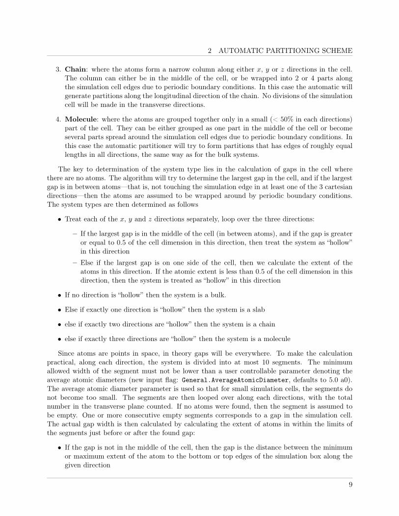
3. Chain: where the atoms form a narrow column along either x, y or z directions in the cell.The column can either be in the middle of the cell, or be wrapped into 2 or 4 parts alongthe simulation cell edges due to periodic boundary conditions. In this case the automatic willgenerate partitions along the longitudinal direction of the chain. No divisions of the simulationcell will be made in the transverse directions.
4. Molecule: where the atoms are grouped together only in a small (< 50% in each directions)part of the cell. They can be either grouped as one part in the middle of the cell or becomeseveral parts spread around the simulation cell edges due to periodic boundary conditions. Inthis case the automatic partitioner will try to form partitions that has edges of roughly equallengths in all directions, the same way as for the bulk systems.
The key to determination of the system type lies in the calculation of gaps in the cell wherethere are no atoms. The algorithm will try to determine the largest gap in the cell, and if the largestgap is in between atoms—that is, not touching the simulation edge in at least one of the 3 cartesiandirections—then the atoms are assumed to be wrapped around by periodic boundary conditions.The system types are then determined as follows
• Treat each of the x, y and z directions separately, loop over the three directions:
– If the largest gap is in the middle of the cell (in between atoms), and if the gap is greateror equal to 0.5 of the cell dimension in this direction, then treat the system as “hollow”in this direction
– Else if the largest gap is on one side of the cell, then we calculate the extent of theatoms in this direction. If the atomic extent is less than 0.5 of the cell dimension in thisdirection, then the system is treated as “hollow” in this direction
• If no direction is “hollow” then the system is a bulk.
• Else if exactly one direction is “hollow” then the system is a slab
• else if exactly two directions are “hollow” then the system is a chain
• else if exactly three directions are “hollow” then the system is a molecule
Since atoms are points in space, in theory gaps will be everywhere. To make the calculationpractical, along each direction, the system is divided into at most 10 segments. The minimumallowed width of the segment must not be lower than a user controllable parameter denoting theaverage atomic diameters (new input flag: General.AverageAtomicDiameter, defaults to 5.0 a0).The average atomic diameter parameter is used so that for small simulation cells, the segments donot become too small. The segments are then looped over along each directions, with the totalnumber in the transverse plane counted. If no atoms were found, then the segment is assumed tobe empty. One or more consecutive empty segments corresponds to a gap in the simulation cell.The actual gap width is then calculated by calculating the extent of atoms in within the limits ofthe segments just before or after the found gap:
• If the gap is not in the middle of the cell, then the gap is the distance between the minimumor maximum extent of the atom to the bottom or top edges of the simulation box along thegiven direction
9
2 AUTOMATIC PARTITIONING SCHEME
• Else if the gap is in the middle of the cell, then gap is equal to the minimum extent of theatoms above the gap and the maximum extent of the atoms below the gap.
This way the extent, gap and type of the system under simulation can be quite robustly esti-mated, and this information are fed into the automatic partitioning subroutines so that the simu-lation cell is divided accordingly.
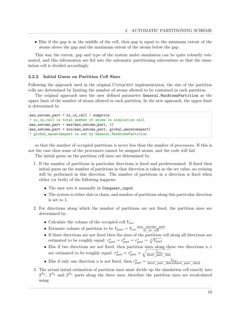
2.2.2 Initial Guess on Partition Cell Sizes
Following the approach used in the original Conquest implementation, the size of the partitioncells are determined by limiting the number of atoms allowed to be contained in each partition.
The original approach uses the user defined parameter General.MaxAtomsPartition as theupper limit of the number of atoms allowed in each partition, In the new approach, the upper limitis determined by
max_natoms_part = ni_in_cell / numprocs! ni_in_cell is total number of atoms in simulation cellmax_natoms_part = max(max_natoms_part, 1)max_natoms_part = min(max_natoms_part, global_maxatomspart)! global_maxatomspart is set by General.MaxAtomsPartition
so that the number of occupied partitions is never less than the number of processors. If this isnot the case then some of the processors cannot be assigned atoms, and the code will fail.
The initial guess on the partition cell sizes are determined by:
1. If the number of partitions in particular directions is fixed and predetermined. If fixed theninitial guess on the number of partitions in that direction is taken as the set value, no resizingwill be performed in this direction. The number of partitions in a direction is fixed wheneither (or both) of the following happens:
• The user sets it manually in Conquest_input
• The system is either slab or chain, and number of partitions along this particular directionis set to 1.
2. For directions along which the number of partitions are not fixed, the partition sizes aredetermined by:
• Calculate the volume of the occupied cell Vocc• Estimate volume of partition to be Vpart = Vocc
max_natoms_partni_in_cell
• If three directions are not fixed then the sizes of the partition cell along all directions areestimated to be roughly equal: rxpart = rypart = rzpart = 3
√Vpart
• Else if two directions are not fixed, then partition sizes along these two directions u, vare estimated to be roughly equal: rupart = rvpart =
√Vocc
fixed_part_dim
• Else if only one direction u is not fixed, then rupart = Voccfixed_part_dim1∗fixed_part_dim2
3. The actual initial estimation of partition sizes must divide up the simulation cell exactly into2Nx , 2Ny and 2Nz parts along the three axes, therefore the partition sizes are recalculatedusing
10

2 AUTOMATIC PARTITIONING SCHEME
! n_parts: number of partitions in 3 directions! n_divs: number of divisions of simulation cell in 3 directions! r_part: partition cell size in 3 directions! FSC: the (fundamental) simulation celldo ii = 1, 3
n_parts(ii) = max(nint(FSC%dims(ii) / r_part(ii)), 1)n_divs(ii) = int_log2(n_parts(ii))n_parts(ii) = 2**n_divs(ii)r_part(ii) = FSC%dims(ii) / real(n_parts(ii),double)
end do
2.2.3 Refining Partition Cell Sizes
The initial estimation of partition sizes are based on the assumption that atoms are uniformlyspread in the occupied region of the simulation cell. This is rarely the case in practice. Hence thepartition sizes needs to be refined so that the number of atoms in each partition stay within thelimit of max_natoms_part. The refinement process is given as follows:
1. Set the number of atoms and support functions in partitions to 0.
2. Loop over all atoms in the simulation cell, the (ix, iy, iz) integer coordinates of the partitioncontaining the particular atom can be obtained from
ix = floor(rxatom/r
xpart)
(1)
iy = floor(ryatom/r
ypart)
(2)
iz = floor(rzatom/r
zpart)
(3)
• From the (ix, iy, iz) coordinates of the partition, work out the corresponding non-cubicHilbert curve index iHilbert, using method presented in section 2.1.
• Increment the atom count and the associated number of support functions in the partitioniHilbert.
• If the number of atoms in a particular partition is greater than max_natoms_part:• Refine partitions: increase the number of divisions—Hilbert curve recursion—Nu of the
direction (u) that has the longest partition cell size: rupart = max(rxpart, rypart, r
zpart). The
number of partitions in direction u is thus doubled to 2(Nu+1).• exit the atom loop and return to step 1.
The process repeats until all partitions has number of atoms less than max_natoms_part. Duringthis process, other important information regarding to the partitions are gathered, such as theCartesian Composite (CC) indices of the partition:
iCC = ixrypartrzpart + iyrzpart + iz
During the actual calculations, it is the CC indices rather than the Hilbert indices that are usedto reference the partitions. Also from the CC indices calculated, work out the atomic index cor-responding to the partitions (see reference [1]) and store the map between the partition atomicindices with global (simulation cell) atomic indices. These are important book-keeping informationallowing each processor to identify local and remote atoms.
11
2 AUTOMATIC PARTITIONING SCHEME
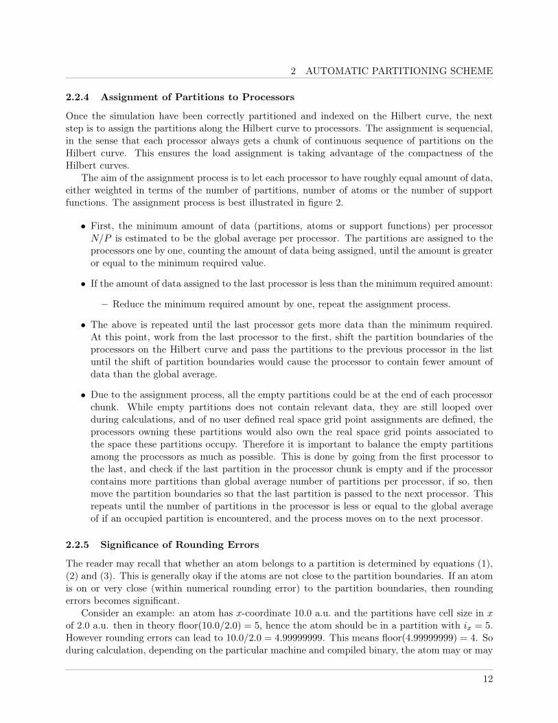
2.2.4 Assignment of Partitions to Processors
Once the simulation have been correctly partitioned and indexed on the Hilbert curve, the nextstep is to assign the partitions along the Hilbert curve to processors. The assignment is sequencial,in the sense that each processor always gets a chunk of continuous sequence of partitions on theHilbert curve. This ensures the load assignment is taking advantage of the compactness of theHilbert curves.
The aim of the assignment process is to let each processor to have roughly equal amount of data,either weighted in terms of the number of partitions, number of atoms or the number of supportfunctions. The assignment process is best illustrated in figure 2.
• First, the minimum amount of data (partitions, atoms or support functions) per processorN/P is estimated to be the global average per processor. The partitions are assigned to theprocessors one by one, counting the amount of data being assigned, until the amount is greateror equal to the minimum required value.
• If the amount of data assigned to the last processor is less than the minimum required amount:
– Reduce the minimum required amount by one, repeat the assignment process.
• The above is repeated until the last processor gets more data than the minimum required.At this point, work from the last processor to the first, shift the partition boundaries of theprocessors on the Hilbert curve and pass the partitions to the previous processor in the listuntil the shift of partition boundaries would cause the processor to contain fewer amount ofdata than the global average.
• Due to the assignment process, all the empty partitions could be at the end of each processorchunk. While empty partitions does not contain relevant data, they are still looped overduring calculations, and of no user defined real space grid point assignments are defined, theprocessors owning these partitions would also own the real space grid points associated tothe space these partitions occupy. Therefore it is important to balance the empty partitionsamong the processors as much as possible. This is done by going from the first processor tothe last, and check if the last partition in the processor chunk is empty and if the processorcontains more partitions than global average number of partitions per processor, if so, thenmove the partition boundaries so that the last partition is passed to the next processor. Thisrepeats until the number of partitions in the processor is less or equal to the global averageof if an occupied partition is encountered, and the process moves on to the next processor.
2.2.5 Significance of Rounding Errors
The reader may recall that whether an atom belongs to a partition is determined by equations (1),(2) and (3). This is generally okay if the atoms are not close to the partition boundaries. If an atomis on or very close (within numerical rounding error) to the partition boundaries, then roundingerrors becomes significant.
Consider an example: an atom has x-coordinate 10.0 a.u. and the partitions have cell size in xof 2.0 a.u. then in theory floor(10.0/2.0) = 5, hence the atom should be in a partition with ix = 5.However rounding errors can lead to 10.0/2.0 = 4.99999999. This means floor(4.99999999) = 4. Soduring calculation, depending on the particular machine and compiled binary, the atom may or may
12
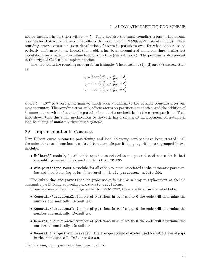
2 AUTOMATIC PARTITIONING SCHEME
not be included in partition with ix = 5. There are also the small rounding errors in the atomiccoordinates that would cause similar effects (for example, x = 9.99999999 instead of 10.0). Theserounding errors causes non even distribution of atoms in partitions even for what appears to beperfectly uniform systems. Indeed this problem has been encountered numerous times during testcalculations on a perfect crystalline bulk Si structure (see 2.4 below). The problem is also presentin the original Conquest implementation.
The solution to the rounding error problem is simple. The equations (1), (2) and (3) are rewrittenas
ix = floor(rxatom/r
xpart + δ
)iy = floor
(ryatom/r
ypart + δ
)iz = floor
(rzatom/r
zpart + δ
)where δ = 10−8 is a very small number which adds a padding to the possible rounding error onemay encounter. The rounding error only affects atoms on partition boundaries, and the addition ofδ ensures atoms within δ a.u. to the partition boundaries are included in the correct partition. Testshave shown that this small modification to the code has a significant improvement on automaticload balancing of uniformly distributed systems.
2.3 Implementation in Conquest
New Hilbert curve automatic partitioning and load balancing routines have been created. Allthe subroutines and functions associated to automatic partitioning algorithms are grouped in twomodules:
• Hilbert3D module, for all of the routines associated to the generation of non-cubic Hilbertspace-filling curves. It is stored in file Hilbert3D.f90
• sfc_partitions_module module, for all of the routines associated to the automatic partition-ing and load balancing tasks. It is stored in file sfc_partitions_module.f90.
The subroutine sfc_partitions_to_processors is used as a drop-in replacement of the oldautomatic partitioning subroutine create_sfc_partitions.
There are several new input flags added to Conquest, these are listed in the tabel below
• General.NPartitionsX: Number of partitions in x, if set to 0 the code will determine thenumber automatically. Default is 0
• General.NPartitionsY: Number of partitions in y, if set to 0 the code will determine thenumber automatically. Default is 0
• General.NPartitionsA: Number of partitions in z, if set to 0 the code will determine thenumber automatically. Default is 0
• General.AverageAtomicDiameter: The average atomic diameter used for estimation of gapsin the simulation cell. Default is 5.0 a.u.
The following input parameter has been modified:
13
2 AUTOMATIC PARTITIONING SCHEME
• General.LoadBalance: A further option =”supportfunctions”= has been added to the optionlist. This flag controls the weighting function used for distributing partitions to the processors.Default is still =”atoms”=
Note that if the user entered a General.NPartitionsX|Y|Z value that is not a power of 2, thenthe code will use the smallest power of 2 integer greater than the user input value as the number ofpartions required in that direction.
The sfc_partitions_module also contains a checking subroutine and an information subroutine.The checking subroutine checks if data has been correctly assigned to the partitions and processors,such as if there are repeats in atomic indices, if the number of atoms in partitions match the totalnumber of atoms in the simulation cell etc. The checks are run every time when the automaticpartitioner is used, so that Conquest can be sure that a valid partition–processor map has beencreated and it can continue to perform actual calculations. The information subroutine dependingon the user controlled global verbosity flag, prints out various statistical information on the partitionand load assignments to processors, so the user can have an idea whether data had been evenlydistributed among the MPI processes.
The user may use the new partitioning scheme without any modifications to his/her Conquest_inputfile used for the old Conquest binary, and should encounter minimal behaviour changes other thandata being allocated differently (hopefully more optimised) internally to the processors.
2.4 Test Results
To test the new non-cubic Hilbert curve partitioner, the computation of the following systemsperformed by the updated Conquest had been compared with results from the old partitioningscheme:
• Bulk Si with 512 atoms, cell dimensions: (41.04 a.u.×41.04 a.u.×41.04 a.u.. Reference code:BulkSi512C
• Bulk Si with 512 atoms, cell dimensions: (82.09 a.u.×82.09 a.u.×10.26 a.u.). Reference code:BulkSi512F
• Bulk Si with 512 atoms, cell dimensions: (656.72 a.u. × 10.26 a.u. × 10.26 a.u.). Referencecode: BulkSi512L
• Slab Si with 2048 atoms in xy plane, located in the middle of the cell, cell dimensions:(82.09 a.u.× 82.09 a.u.× 92.35 a.u.). Reference code: SlabSi2048M
• Slab Si with 2048 atoms in xy plane, located at the bottom of the cell, half of the atomswrapped by periodic boundary condition to the top of the cell, cell dimensions: (82.09 a.u.×82.09 a.u.× 92.35 a.u.). Reference code: SlabSi2048W
• Ge hut cluster on Si substrate (slab) with 5333 atoms, slab spans the xy-plane, and locatedat the bottom of the cell, cell dimensions: (164.18 a.u.× 205.22 a.u.× 51.31 a.u.). See figure3. Reference code: GeSi5333
• Ge hut cluster on Si substrate (slab) with 22746 atoms, slab spans the xy-plane, and located atthe top of the cell and wrapped around to the bottom of the cell, cell dimensions: (328.36 a.u.×328.36 a.u.× 89.79 a.u.). See figure 4. Reference code: GeSi22746
14
2 AUTOMATIC PARTITIONING SCHEME
• Ge hut cluster on Si substrate (slab) with 39130 atoms, slab spans the xy-plane, and located atthe top of the cell and wrapped around to the bottom of the cell, cell dimensions: (328.36 a.u.×328.36 a.u.× 97.48 a.u.). See figure 5. Reference code: GeSi22746
• DNA in water with 3439 atoms. This is used to test whether the load balance weighting by thesupport functions has any performance improvements over weighting by the atoms. Referencecode: DNAH2O3439
All test results are based on non-self-consistent single point energy minimisation calculations,with auxiliary matrix tolerance of 10−4 Ha. All calculations were done on HECToR phase 3. Thenew non-cubic Hilbert partitioner is referred to in below as SFC-1.6 (revision 1.6 of the new space-filling-curve implementation); and the original Conquest is referred to as r162 (the 162-nd revisionin the source code trunk—the most recent released version). Both SCF-1.6 and r162 were compiledwith Cray compiler suit PrgEnv-cray/4.0.46 with xt-libsci/12.0.00. The optimisation flag forthe compiler was set at -O3.
2.4.1 Performance in Relation to Cell Shapes
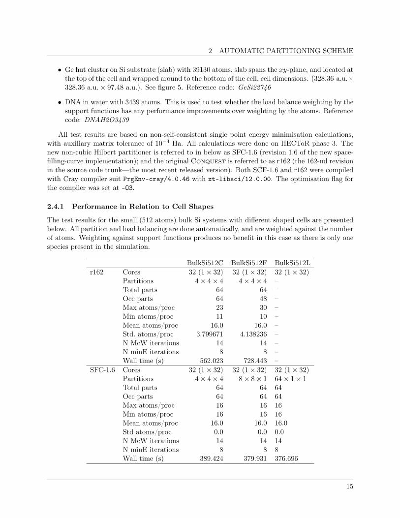
The test results for the small (512 atoms) bulk Si systems with different shaped cells are presentedbelow. All partition and load balancing are done automatically, and are weighted against the numberof atoms. Weighting against support functions produces no benefit in this case as there is only onespecies present in the simulation.
BulkSi512C BulkSi512F BulkSi512Lr162 Cores 32 (1× 32) 32 (1× 32) 32 (1× 32)
Partitions 4× 4× 4 4× 4× 4 –Total parts 64 64 –Occ parts 64 48 –Max atoms/proc 23 30 –Min atoms/proc 11 10 –Mean atoms/proc 16.0 16.0 –Std. atoms/proc 3.799671 4.138236 –N McW iterations 14 14 –N minE iterations 8 8 –Wall time (s) 562.023 728.443 –
SFC-1.6 Cores 32 (1× 32) 32 (1× 32) 32 (1× 32)Partitions 4× 4× 4 8× 8× 1 64× 1× 1Total parts 64 64 64Occ parts 64 64 64Max atoms/proc 16 16 16Min atoms/proc 16 16 16Mean atoms/proc 16.0 16.0 16.0Std atoms/proc 0.0 0.0 0.0N McW iterations 14 14 14N minE iterations 8 8 8Wall time (s) 389.424 379.931 376.696
15
2 AUTOMATIC PARTITIONING SCHEME
The r162 version failed to assign atoms to all processors for BulkSi512L, and stopped before anypartition data can be printed. The extreme difference in the cell dimensions had broken the loadbalancing algorithm using the standard cubic Hilbert curves, as far too many partitions are beingcreated in the transverse directions. Significant slow down can be observed going from the cubic cellBulkSi512C to the flat cell BulkSi512F, as empty partitions are being created due inflexibility of thecubic 3D Hilbert curve. The new partitioning scheme however produced optimal load balancing inall three cell shapes. The correction to the rounding error mentioned in section 2.2.5 is also evidentwhen comparing the results for BulkSi512C, where both partitioning schemes used the same numberof partitions and cubic Hilbert curve. The new scheme correctly corrected the placement of atomsin partitions, resulting significant improvements in performance.
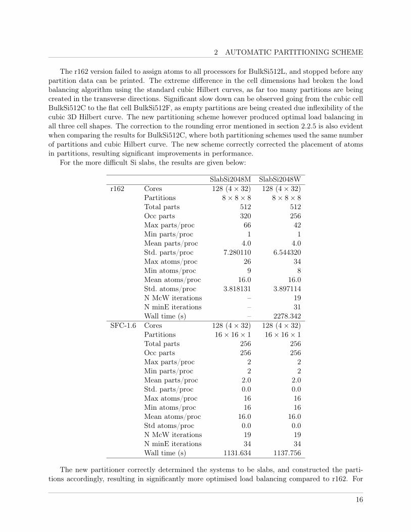
For the more difficult Si slabs, the results are given below:
SlabSi2048M SlabSi2048Wr162 Cores 128 (4× 32) 128 (4× 32)
Partitions 8× 8× 8 8× 8× 8Total parts 512 512Occ parts 320 256Max parts/proc 66 42Min parts/proc 1 1Mean parts/proc 4.0 4.0Std. parts/proc 7.280110 6.544320Max atoms/proc 26 34Min atoms/proc 9 8Mean atoms/proc 16.0 16.0Std. atoms/proc 3.818131 3.897114N McW iterations – 19N minE iterations – 31Wall time (s) – 2278.342
SFC-1.6 Cores 128 (4× 32) 128 (4× 32)Partitions 16× 16× 1 16× 16× 1Total parts 256 256Occ parts 256 256Max parts/proc 2 2Min parts/proc 2 2Mean parts/proc 2.0 2.0Std. parts/proc 0.0 0.0Max atoms/proc 16 16Min atoms/proc 16 16Mean atoms/proc 16.0 16.0Std atoms/proc 0.0 0.0N McW iterations 19 19N minE iterations 34 34Wall time (s) 1131.634 1137.756
The new partitioner correctly determined the systems to be slabs, and constructed the parti-tions accordingly, resulting in significantly more optimised load balancing compared to r162. For
16
2 AUTOMATIC PARTITIONING SCHEME
SlabSi2048M, r612 crashed due to OOM error on HECToR. Due to the fact that the phase 3 HEC-ToR has only 1GB of memory per core, it is easy to go over the limits if the load balance is notsufficiently good. In this case, the problem did not come from too many atoms being allocated toone processor, but came from the fact that too many empty partitions were produced and someprocessors got too many empty partitions. This fact can be observed from the large disparity be-tween the maximum and minimum number of partitions per processor (66 vs. 1). The result is toomany integration block points are being assigned to a particular processor, resulting in OOM error.
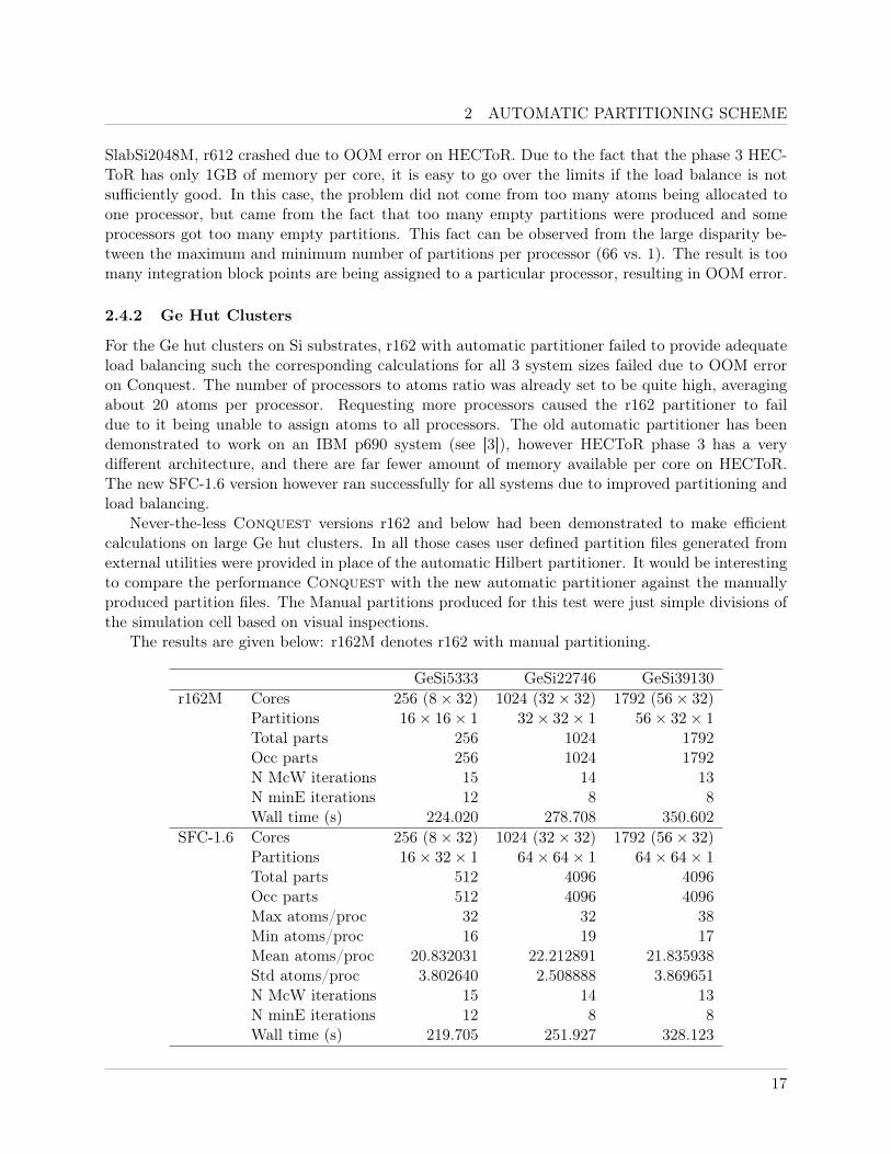
2.4.2 Ge Hut Clusters
For the Ge hut clusters on Si substrates, r162 with automatic partitioner failed to provide adequateload balancing such the corresponding calculations for all 3 system sizes failed due to OOM erroron Conquest. The number of processors to atoms ratio was already set to be quite high, averagingabout 20 atoms per processor. Requesting more processors caused the r162 partitioner to faildue to it being unable to assign atoms to all processors. The old automatic partitioner has beendemonstrated to work on an IBM p690 system (see [3]), however HECToR phase 3 has a verydifferent architecture, and there are far fewer amount of memory available per core on HECToR.The new SFC-1.6 version however ran successfully for all systems due to improved partitioning andload balancing.
Never-the-less Conquest versions r162 and below had been demonstrated to make efficientcalculations on large Ge hut clusters. In all those cases user defined partition files generated fromexternal utilities were provided in place of the automatic Hilbert partitioner. It would be interestingto compare the performance Conquest with the new automatic partitioner against the manuallyproduced partition files. The Manual partitions produced for this test were just simple divisions ofthe simulation cell based on visual inspections.
The results are given below: r162M denotes r162 with manual partitioning.
GeSi5333 GeSi22746 GeSi39130r162M Cores 256 (8× 32) 1024 (32× 32) 1792 (56× 32)
Partitions 16× 16× 1 32× 32× 1 56× 32× 1Total parts 256 1024 1792Occ parts 256 1024 1792N McW iterations 15 14 13N minE iterations 12 8 8Wall time (s) 224.020 278.708 350.602
SFC-1.6 Cores 256 (8× 32) 1024 (32× 32) 1792 (56× 32)Partitions 16× 32× 1 64× 64× 1 64× 64× 1Total parts 512 4096 4096Occ parts 512 4096 4096Max atoms/proc 32 32 38Min atoms/proc 16 19 17Mean atoms/proc 20.832031 22.212891 21.835938Std atoms/proc 3.802640 2.508888 3.869651N McW iterations 15 14 13N minE iterations 12 8 8Wall time (s) 219.705 251.927 328.123
17
3 MOLECULAR DYNAMICS WITH DYNAMIC REASSIGNMENT
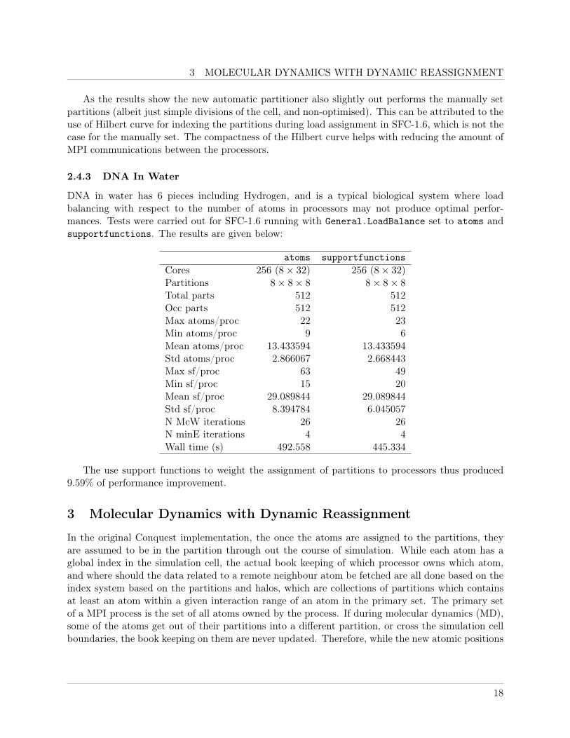
As the results show the new automatic partitioner also slightly out performs the manually setpartitions (albeit just simple divisions of the cell, and non-optimised). This can be attributed to theuse of Hilbert curve for indexing the partitions during load assignment in SFC-1.6, which is not thecase for the manually set. The compactness of the Hilbert curve helps with reducing the amount ofMPI communications between the processors.
2.4.3 DNA In Water
DNA in water has 6 pieces including Hydrogen, and is a typical biological system where loadbalancing with respect to the number of atoms in processors may not produce optimal perfor-mances. Tests were carried out for SFC-1.6 running with General.LoadBalance set to atoms andsupportfunctions. The results are given below:
atoms supportfunctionsCores 256 (8× 32) 256 (8× 32)Partitions 8× 8× 8 8× 8× 8Total parts 512 512Occ parts 512 512Max atoms/proc 22 23Min atoms/proc 9 6Mean atoms/proc 13.433594 13.433594Std atoms/proc 2.866067 2.668443Max sf/proc 63 49Min sf/proc 15 20Mean sf/proc 29.089844 29.089844Std sf/proc 8.394784 6.045057N McW iterations 26 26N minE iterations 4 4Wall time (s) 492.558 445.334
The use support functions to weight the assignment of partitions to processors thus produced9.59% of performance improvement.
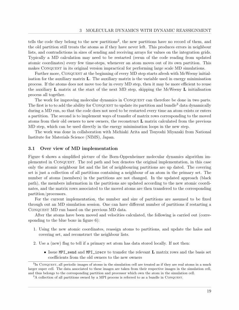
3 Molecular Dynamics with Dynamic Reassignment
In the original Conquest implementation, the once the atoms are assigned to the partitions, theyare assumed to be in the partition through out the course of simulation. While each atom has aglobal index in the simulation cell, the actual book keeping of which processor owns which atom,and where should the data related to a remote neighbour atom be fetched are all done based on theindex system based on the partitions and halos, which are collections of partitions which containsat least an atom within a given interaction range of an atom in the primary set. The primary setof a MPI process is the set of all atoms owned by the process. If during molecular dynamics (MD),some of the atoms get out of their partitions into a different partition, or cross the simulation cellboundaries, the book keeping on them are never updated. Therefore, while the new atomic positions
18
3 MOLECULAR DYNAMICS WITH DYNAMIC REASSIGNMENT
tells the code they belong to the new partitions2, the new partitions have no record of them, andthe old partition still treats the atoms as if they have never left. This produces errors in neighbourlists, and contradictions in sizes of sending and receiving arrays for values on the integration grids.Typically a MD calculation may need to be restarted (rerun of the code reading from updatedatomic coordinates) every few time-steps, whenever an atom moves out of its own partition. Thismakes Conquest in its original version impractical for performing large scale MD simulations.
Further more, Conquest at the beginning of every MD step starts afresh with McWeeny initial-isation for the auxiliary matrix L. The auxiliary matrix is the variable used in energy minimisationprocess. If the atoms does not move too far in every MD step, then it may be more efficient to reusethe auxiliary L matrix at the start of the next MD step, skipping the McWeeny L initialisationprocess all together.
The work for improving molecular dynamics in Conquest can therefore be done in two parts.The first is to to add the ability for Conquest to update its partition and bundle3 data dynamicallyduring a MD run, so that the code does not need to be restarted every time an atom exists or entersa partition. The second is to implement ways of transfer of matrix rows corresponding to the movedatoms from their old owners to new owners, the reconstruct L matrix calculated from the previousMD step, which can be used directly in the energy minimisation loops in the new step.
The work was done in collaboration with Michiaki Arita and Tsuyoshi Miyazaki from NationalInstitute for Materials Science (NIMS), Japan.
3.1 Over view of MD implementation
Figure 6 shows a simplified picture of the Born-Oppenheimer molecular dynamics algorithm im-plemented in Conquest. The red path and box denotes the original implementation, in this caseonly the atomic neighbour list and the list of neighbouring partitions are up dated. The coveringset is just a collection of all partitions containing a neighbour of an atom in the primary set. Thenumber of atoms (members) in the partitions are not changed. In the updated approach (blackpath), the members information in the partitions are updated according to the new atomic coordi-nates, and the matrix rows associated to the moved atoms are then transfered to the correspondingpartition/processors.
For the current implementation, the number and size of partitions are assumed to be fixedthrough out an MD simulation session. One can have different number of partitions if restarting aConquest MD run based on the previous MD data.
After the atoms have been moved and velocities calculated, the following is carried out (corre-sponding to the blue boxe in figure 6):
1. Using the new atomic coordinates, reassign atoms to partitions, and update the halos andcovering set, and reconstruct the neighbour lists.
2. Use a (new) flag to tell if a primary set atom has data stored locally. If not then:
• Issue MPI_send and MPI_irecv to transfer the relevant L matrix rows and the basis setcoefficients from the old owners to the new owners
2In Conquest, all periodic images of atoms in the simulation cell are treated as if they are real atoms in a muchlarger super cell. The data associated to these images are taken from their respective images in the simulation cell,and thus belongs to the corresponding partition and processor which own the atom in the simulation cell.
3A collection of all partitions owned by a MPI process is referred to as a bundle in Conquest.
19
3 MOLECULAR DYNAMICS WITH DYNAMIC REASSIGNMENT
3. Reorder the local rows (not including the remote rows being fetched in step 2.) of L ac-cording to the new indices calculated from step 1. This can be done in parallel to the MPIcommunications initiated in step 2.
4. After the MPI communications have finished, the reindexed L matrix part on the processoris reconstructed from the reordered local rows and received received rows.
Once the L matrix has been reconstructed with up to date neighbour lists, it can then be fedinto the DFT routines for the next round of MD loop.
3.2 Update Members Information
After the calculation of DFT ground states and movement of atoms during MD step n, each processorknows:
• The updated coordinates of atoms in its old primary set
• The updated covering set (neighbour lists) corresponding to the old primary set
• The displacement of atoms in the primary set (from step n− 1 to n)
There are situation where an atom has wondered out of the simulation cell, and therefore,becomes an “periodic image”. It must be folded back into the simulation cell according to periodicboundary conditions, and be assigned to the new partition accordingly.
To update the member information, each processor must do the following:
• Loop over all atoms in the simulation cell, recalculate which partition does each atom belongto, any atom that have existed the simulation cell are assigned partitions corresponding to itsperiodic image in the cell
• Reconstruct the partitions, and update the local atom sequence mappings for all proces-sors. The atom sequences are arranged in the order of bundles (set of partitions owned by aprocessor)–partitions–atoms
• From the new processor-partition-atom maps, reconstruct the global atomic index to bundleatomic index mappings. At the same time, remember the old mappings, as it will be used forrearranging various data arrays whose elements are still ordered according to the old maps
• Rearrange the atomic coordinates, velocity and species arrays according to the new atomicbundle indices.
• Update the new primary set
• Update the neighbour list and the covering set
After the member information is updated, the code can either continue onto a new moleculardynamics step, with L rebuilt from scratch, and pass through the McWeeny initialisation and earlyenergy minimisation (preparation) steps; or more perhaps more efficiently reconstruct the L matrixfrom the current MD step using the updated member information, and use it as the initial inputfor the energy minimisation steps in the next MD step. This way, both McWeeny iteration andearly energy minimisation preparations may be skipped, thus improving the running time of theMD simulation. The section below describes how L may be rebuilt.
20

3 MOLECULAR DYNAMICS WITH DYNAMIC REASSIGNMENT
3.3 Reconstruct L Matrix
After the member information have been updated, in theory all of the required L matrix datahas already been computed by the previous MD step. The L matrix is piece-wisely stored on allparticipating processors, with format dependent on the primary and covering set information. Asthe primary and covering set has changed, the way Lmatrix is stored must also change to correspondto the new member informations for the code to run correctly. This section gives a brief explanationon how is done.
The L matrix is stored in rows on the processors. The row are indexed by atoms and theircorresponding support functions. Only the matrix elements with column index being the neighboursof i are stored in each row.
Each processor must first work out which of its own rows (atoms) now belongs to the primarysets of other processors, and which atom now in its primary set is was a member of the primaryset on another processor. The processors not only has to send the relevant rows of L, it also has tosend the information on the global atomic index of the row (i.e. which exact row in the global L) itis sending, how many rows, and global atomic indices of neighbours j in each row. Otherwise unlikein the original Conquest implementation where the member data never changes, the processorswould not be able to find out the identity of the remote matrix data it received because the memberdata has changed while the data received was still arranged using the old format. Therefore in orderto reorder for each processor to the matrix rows correctly, the exact format information about theL matrix needs to be sent and received before the matrix rows are being sent, which records:
• The number of atoms in the old primary set corresponding to the Lmatrix before its reordering
• The α indices (support function indices) corresponding to each atom i, indexing the matrixelement Liαjβ
• The number of (old) neighbours j of each atom i, which corresponds to the length of each rowin L
• The global ids of all the neighbours j of atom i in the simulation
• The length of each Liαjβ row (the number of combined index jβ)
• The beginning location in the L matrix array for each row, indexed by i
• The support function β indices of each of neighbours j of atom i
• The displacements between atoms i and the neighbours j of the L matrix not yet been re-ordered, and with the atoms indexed in the covering set-partition-atom indices of the previousMD step. This information is important for reordering the matrix elements for the currentMD step.
The above is grouped into a structure type InfoL, and will be sent to and received by therelevant processor before the matrix data is sent. After this the relevant matrix rows are sent,using MPI_irecv and MPI_send pair. The part of L is first reordered using the updated memberinformation, and once the relevant data from the remote matrix row has been received they areadded to the local matrix to complete the reconstruction of L.
21

3 MOLECULAR DYNAMICS WITH DYNAMIC REASSIGNMENT
To reorder the local L matrix, the goal is to identify the row atoms and their neighbours storedin the old matrix format and correspond them to the atoms in the new covering set. The followingsteps are taken:
• Loop over the old primary atoms iold, rows of local L (number from InfoL)
– Loop over the current primary atoms inew and match via global id which inew correspondsto iold and get the the new bundle index for this atom: inew
– Get the atomic displacement of inew from the previous step, which are stored duringvelocity-verlet routine when moving atoms.
– Loop over the old neighbours jold (number from InfoL), at the moment these atoms areunidentified, the goal of this loop is to find their id in the updated neighbour list.
∗ Get the atomic displacement of jold from data stored in velocity-verlet routine∗ Get the current position of jnew, calculated using the current position of inew, the
displacement of iold during MD and the old atomic displacements between iold andjold stored in InfoL
∗ From the position of jnew find the partition in the (current) covering set this atombelongs to
∗ Loop over the atoms in that partition, and use the global id of jold the current bundlelabeling for jnew
∗ Reorder the L matrix elements
The remote matrix elements are constructed into the new formatted L matrix in the same way,by identifying the atoms associated to the row and column indices of the received matrix rows inthe new covering set, and then assign the matrix rows to their appropriate places accordingly
3.4 Test Results
The tests were carried out to find out the stability of the implemented MD routines when runningon HECToR. The code was again compiled with Cray compiler suit PrgEnv-cray/4.0.46 withxt-libsci/12.0.00. The optimisation flag for the compiler was set at -O3.
The test systems are water (ice) boxes of various sizes. The molecular dynamics settings werealways set with:
• Initial ionic temperature: 300 K
• Time step-size: 0.5 fs
• DFT Functional: PW92 (LDA)
• Self-consistency: Mixed energy minimisation and charge self-consistency scheme
3.4.1 Stability
First the stability of the MD algorithm was tested. Conquest was run on 32 cores (1 node) onHECToR phase 3, for MD simulation of a 768 atoms water box. The first run without reusingthe L matrix, starting from McWeeny initialisations at every time step. This is the way the orig-inal Conquest implements MD, with the only difference being the member data is now updated
22
3 MOLECULAR DYNAMICS WITH DYNAMIC REASSIGNMENT
after every MD step, so the code would not stop if an atom crosses a partition boundary. Theresults were then compared with the MD calculation run that does reuse the L matrix, and skipsthe entire McWeeny initialisation steps and early energy minimisation preparations. The L matrixtolerance, the criteria for finishing the energy minimisation procedure was set to 10−3. Originallythe simulation time was set to be 800 iterations (400 fs). However, due to the slow speed of thecalculation with using McWeeny iterations for every time step, only 136 MD steps were completedin 12 hours. 32 cores were already quite large number of cores for a 768 atoms system, and in-creasing the number of cores beyond 64 atoms would result in poor load balancing as well as largeincreases in communication-to-computation ratio. In any case the speed up of calculation requiredfor completing 400+ step computations will need to be 4 to 5 times, this cannot be achieved byincreasing the number of cores before the atoms in the simulation cell run out. Therefore, a longtest run on HECToR for the MD calculation with McWeeny initialisation at every time step wasconsidered to be impractical. Never-the-less long MD runs for a small 8 atom Si cell with the sameConquest settings were performed on the NIMS Simulator 1 (Intel Xeon processor Nehalem-EP(2.8 GHz), 4 cores/ node, 2.85GB per core) in Japan, the results of which are also presented in thissection below.
Figure 7 shows the total energy vs. simulation time results of the MD runs on the 768 atomswater box carried out using McWeeny initialisation and that reusing the L matrix at each step. Thesimulation was carried out for 100 steps. Significant oscillations in total energy was observed for theboth simulation. For both simulations the amplitude of the oscillation decreased over simulationtime, with the amplitude dropping faster for the calculation with reused L. The mean energy ofthe “McWeeny” calculation stayed constant, while the “reuseL” result showed a clear drift, whichgradually turned constant at a lower energy.
The oscillations observed for the “McWeeny” calculations seemed to be dependent on the typeof systems. The results shown in figure 8 corresponds to that of the test calculations performed onSi 8 atoms cell by collaborators from NIMS Japan using exactly the same code demonstrated thatthe energy of MD simulation with McWeeny initialisation being used at every step remained largelyconstant, with only very small amount oscillations about the mean value. However the energy driftin “reuseL” results follow the same trend as the corresponding results obtained for the water box onHECToR.
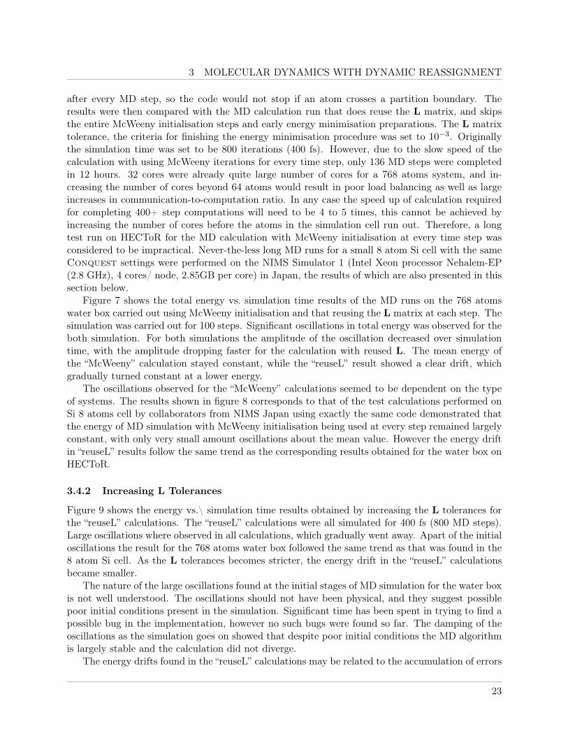
3.4.2 Increasing L Tolerances
Figure 9 shows the energy vs.\ simulation time results obtained by increasing the L tolerances forthe “reuseL” calculations. The “reuseL” calculations were all simulated for 400 fs (800 MD steps).Large oscillations where observed in all calculations, which gradually went away. Apart of the initialoscillations the result for the 768 atoms water box followed the same trend as that was found in the8 atom Si cell. As the L tolerances becomes stricter, the energy drift in the “reuseL” calculationsbecame smaller.
The nature of the large oscillations found at the initial stages of MD simulation for the water boxis not well understood. The oscillations should not have been physical, and they suggest possiblepoor initial conditions present in the simulation. Significant time has been spent in trying to find apossible bug in the implementation, however no such bugs were found so far. The damping of theoscillations as the simulation goes on showed that despite poor initial conditions the MD algorithmis largely stable and the calculation did not diverge.
The energy drifts found in the “reuseL” calculations may be related to the accumulation of errors
23
3 MOLECULAR DYNAMICS WITH DYNAMIC REASSIGNMENT
during successive MD steps. The resetting of L matrix for theWhile this dCSE project has completed, the investigation into the problems in MD simulations
is on going by the collaborative development team of Conquest.
3.4.3 Computational Costs
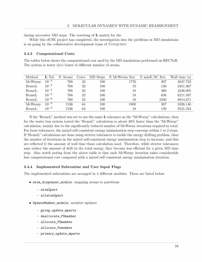
The tables below shows the computational cost used by the MD simulations performed on HECToR.The system is water (ice) boxes of different number of atoms,
Method L Tol. N Atoms Cores MD Steps N McWeeny Iter. N minE/SC Iter. Wall time (s)McWeeny 10−3 768 32 100 1776 307 4047.732ReuseL 10−3 768 32 100 18 130 2451.367ReuseL 10−4 768 32 100 18 366 4246.005ReuseL 10−5 768 32 100 18 656 6211.387ReuseL 10−6 768 32 100 18 1030 8814.671McWeeny 10−3 1536 64 100 1800 307 5826.146ReuseL 10−3 1536 64 100 18 130 3531.344
If the “ReuseL” method was set to use the same L tolerance as the “McWeeny” calculations, thenfor the water box system tested the “ReuseL” calculation is about 40% faster than the “McWeeny”calculation, mainly due to the significantly reduced number of McWeeny iterations required in total.For loose tolerances, the mixed self-consistent energy minimisation step converge within 1 or 2 steps.If “ReuseL” calculations are done using stricter tolerances to tackle the energy drifting problem, thenthe number of iterations in the mixed self-consistent energy minimisation step to increase, and thisare reflected it the amount of wall time those calculation used. Therefore, while stricter tolerancesmay reduce the amount of drift in the total energy, they become less efficient for a given MD timestep. Also worth noting from the above table is that each McWeeny iteration takes considerableless computational cost compared with a mixed self consistent energy minimisation iteration.
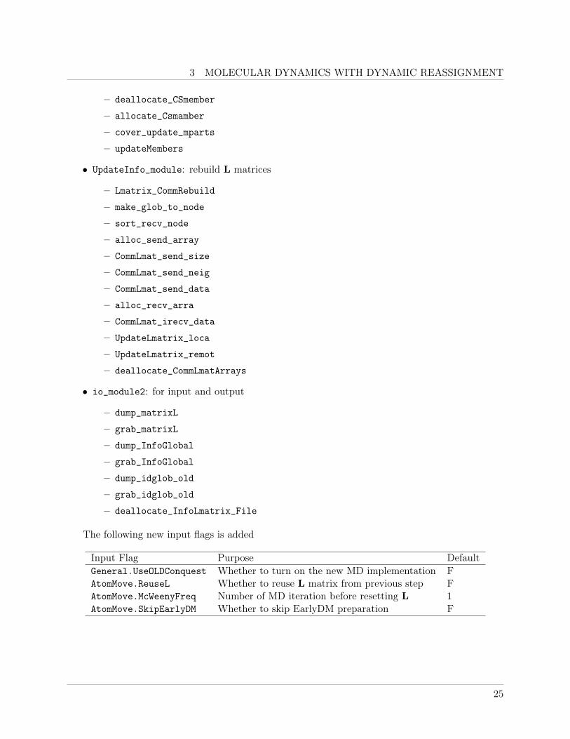
3.4.4 Implemented Subroutine and User Input Flags
The implemented subroutines are arranged in 4 different modules. These are listed below:
• atom_dispenser_module: mapping atoms to partitions
– atom2part
– allatom2part
• UpdateMember_module: member updates
– group_update_mparts
– deallocate_PSmember
– allocate_PSmember
– allocate_Psmember
– primary_update_mparts
24
3 MOLECULAR DYNAMICS WITH DYNAMIC REASSIGNMENT
– deallocate_CSmember
– allocate_Csmamber
– cover_update_mparts
– updateMembers
• UpdateInfo_module: rebuild L matrices
– Lmatrix_CommRebuild
– make_glob_to_node
– sort_recv_node
– alloc_send_array
– CommLmat_send_size
– CommLmat_send_neig
– CommLmat_send_data
– alloc_recv_arra
– CommLmat_irecv_data
– UpdateLmatrix_loca
– UpdateLmatrix_remot
– deallocate_CommLmatArrays
• io_module2: for input and output
– dump_matrixL
– grab_matrixL
– dump_InfoGlobal
– grab_InfoGlobal
– dump_idglob_old
– grab_idglob_old
– deallocate_InfoLmatrix_File
The following new input flags is added
Input Flag Purpose DefaultGeneral.UseOLDConquest Whether to turn on the new MD implementation FAtomMove.ReuseL Whether to reuse L matrix from previous step FAtomMove.McWeenyFreq Number of MD iteration before resetting L 1AtomMove.SkipEarlyDM Whether to skip EarlyDM preparation F
25

4 MISCELLANEOUS REMARKS
3.5 Extended Lagrangian Born-Oppenheimer MD
As the test have show that despite a dramatic increase in speed when reusing L matrix for lowertolerances, the stability of the calculations required a stricter L matrix tolerance, which reducedthe effectiveness in performance improvements when reusing L.
One possible solution was found by extending the existing Conquest Bon-Oppenheimer MDto use the extended Lagrangian formalism[6], which incorporates additional electronic degrees offreedom into the Born-Oppenheimer Lagrangian. L matrix is reused at every MD step, and noMcWeeny initialisation iterations are required for the extended Lagrangian Born-Oppenheimer MD.
Result of a preliminary test calculation using Conquest with the extended Lagrangian formal-ism performed on an 8 atom Si cell is shown in figure 10. The results show that extended Lagrangianformalism produced virtually no energy drift when using a loose tolerance of 10−3.
The computational costs of the extend Lagrangian Born-Oppenheimer MD for the 8 atoms Sicell is compared with the “McWeeny” and “ReuseL” methods in the table below:
Method L Tol. MD Steps N McWeeny Iter. N minE/SC Iter.Ex. Lag. 1o−3 2000 17 4766McWeeny 10−3 2000 34000 > 20000ReuseL 10−3 2000 17 >2000ReuseL 10−4 2000 17 ≈ 4000ReuseL 10−5 2000 17 7476ReuseL 10−6 2000 17 16677ReuseL 10−7 2000 17 28298
The results indicate that while the Extended Lagrangian formalism is more complicated (hencemore expensive per MD step than “ReuseL” method) and takes more iterations to for the energyto converge than “ReuseL” method using the same L tolerance, the extended Lagrangian methodoffered much more superior performance in stability of the MD simulation. The new method is stillsignificantly faster than the method involving resetting L with McWeeny initialisation at every MDstep.
The research in this topic is on-going, and it is beyond the scope of this dCSE project.
4 Miscellaneous Remarks
During running tests on the Hilbert automatic partitioner implementation on HECToR, errors wereencountered which was traced to be caused by the optimisation settings during compilation of Con-quest using Cray compiler (PrgEnv-cray/4.0.46). Setting optimiser flags to either -O2 and -O3caused error in the atomic indices, while turning off optimisation made the error disappear. Furtheranalyst showed this may have been caused by the optimiser trying to merge or swap several linesof code—inserting a print statement between the incident lines fixed the bug (with the optimiserset to -O3).
The code was properly fixed eventually by rewriting the part of code that was causing theproblem in a different way (while doing the same logical functions).
26
6 ACKNOWLEDGEMENT
5 Summary and Conclusion
The goal of this dCSE project is to:
1. Implement a more flexible Hilbert partitioning algorithm in Conquest, in order to improvethe user friendliness of the code in general and load balancing when running on HECToR.
2. Change the existing molecular dynamics code in Conquest to include ability to dynamicallyreassign atoms to partitions, thus allowing the code to perform molecular dynamics simulationswithout needing to restart in frequent intervals. Furthermore, allow the code to use thecalculated L matrix from the previous MD step in order to speed up the simulation.
Objective 1 has been successfully achieved. A solution for generating flexible non-cubic Hilbertcurves has been found, and the associated automatic partitioning algorithms have been implementedin Conquest. The new automatic partitioning algorithm shows significant improvement in bothload balancing performances and functionality over the original implementation. It allowed users tomanually set partitions in any given direction at will. Tests have shown that due to the use of Hilbertcurves the partitioning algorithm out-performed the external utility that was traditionally used byusers to manually set partitions and distribute data to processors, and thus can potentially become areplacement over the existing external utility. The partitioner in full-auto mode also performed wellcompared with the original implementation. In particular the new automatic partitioning schemeallowed calculations to be performed efficiently for awkward systems on HECToR with minimal userinput, where the original automatic partitioner would fail.
Objective 2 has been achieved with partial success. All of the proposed implementations re-lated to MD has been successfully implemented. Most importantly Conquest can now performstable MD simulations for indefinite number of steps without the need to restart the job. Interms of performance improvements, however, while reusing L reduces the computation cost from40%(water)-90%(Si) compared with initialising the matrix at every time step, significant energydrift where observed. Tightening up computational tolerances during MD simulations helped toreduce the energy drift, but at a great cost to overall computational time. Large initial oscillationsin total energy was also observed during doing test calculations on water boxes. The investigationon this problem is still on-going by the Conquest development team. Due to the energy drift andoscillation issues with the current MD implementation, the MD simulation of large GramicidinAembedded lipid bilayer originally proposed for the project was not performed.
The recent works indicated that solution to the problems discovered in MD may be solved byemploying the extended Lagrangian Born-Oppenheimer formalism. While the investigation on thistopic is still on-going, preliminary studies have shown positive results.
The work on the new Hilbert partitioner has been submitted into Conquest trunk, and isavailable to all users of Conquest.
6 Acknowledgement
The Author wish to thank Michiaki Arita and Tsuyoshi Miyazaki for their contribution to the workon implementing the improved molecular dynamics algorithms in Conquest.
This project was funded under the HECToR Distributed Computational Science and Engineer-ing (CSE) Service operated by NAG Ltd. HECToR—A Research Councils UK High End Computing
27
REFERENCES
Service—is the UK’s national supercomputing service, managed by EPSRC on behalf of the par-ticipating Research Councils. Its mission is to support capability science and engineering in UKacademia. The HECToR supercomputers are managed by UoE HPCx Ltd and the CSE SupportService is provided by NAG Ltd. http://www.hector.ac.uk
References
[1] D. R. Bowler, T. Miyazaki, and M. J. Gillan. Parallel sparse matrix multiplication for linearscaling electronic structure calculations. Comput. Phys. Commun., 137(2):255–273, June 2001.
[2] D. R. Bowler, T. Miyazaki, and M. J. Gillan. Recent progress in linear scaling ab initio electronicstructure techniques. J. Phys.: Condens. Matter, 14(11):2781, 2002.
[3] V. Brázdová and D. R. Bowler. Automatic data distribution and load balancing with space-fillingcurves: implementation in CONQUEST. J. Phys.: Condens. Matter, 20(27):275223, 2008.
[4] F. Gray. Pulse code communication, 1953.
[5] W. Kohn and L. J. Sham. Self-consistent equations including exchange and correlation effects.Phys. Rev., 140(4A):A1133, 1965.
[6] A. M. N. Niklasson. Extended born-oppenheimer molecular dynamics. Phys. Rev. Lett.,100(12):123004–, Mar. 2008.
[7] H. Sagan. Space Filling Curves. Springer, 1994.
[8] J. Skilling. In G. Erickson and Y. Zhai, editors, Bayesian Inference and Maximum EntropyMethods in Science and Engineering: 23rd Int. Workshop, number CP707, page 381–7, NewYork, 2004. American Institute of Physics.
28
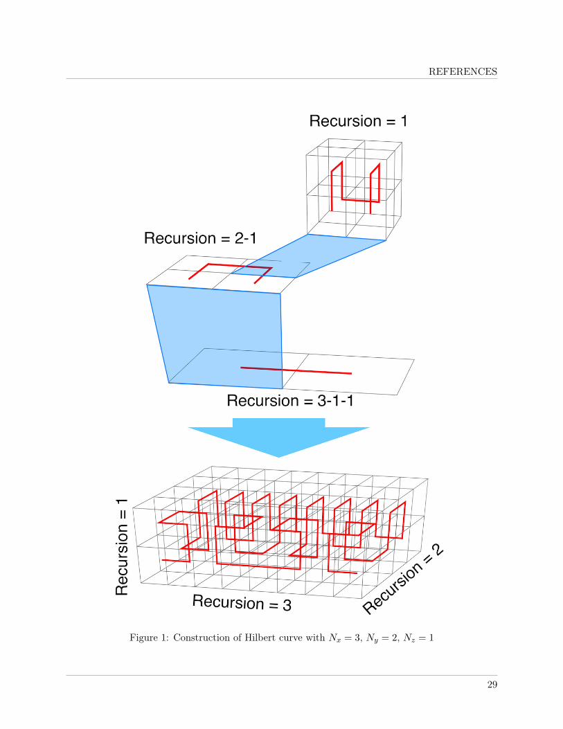
REFERENCES
Figure 1: Construction of Hilbert curve with Nx = 3, Ny = 2, Nz = 1
29

REFERENCES
Figure 2: Assignment of partitions to processors
30
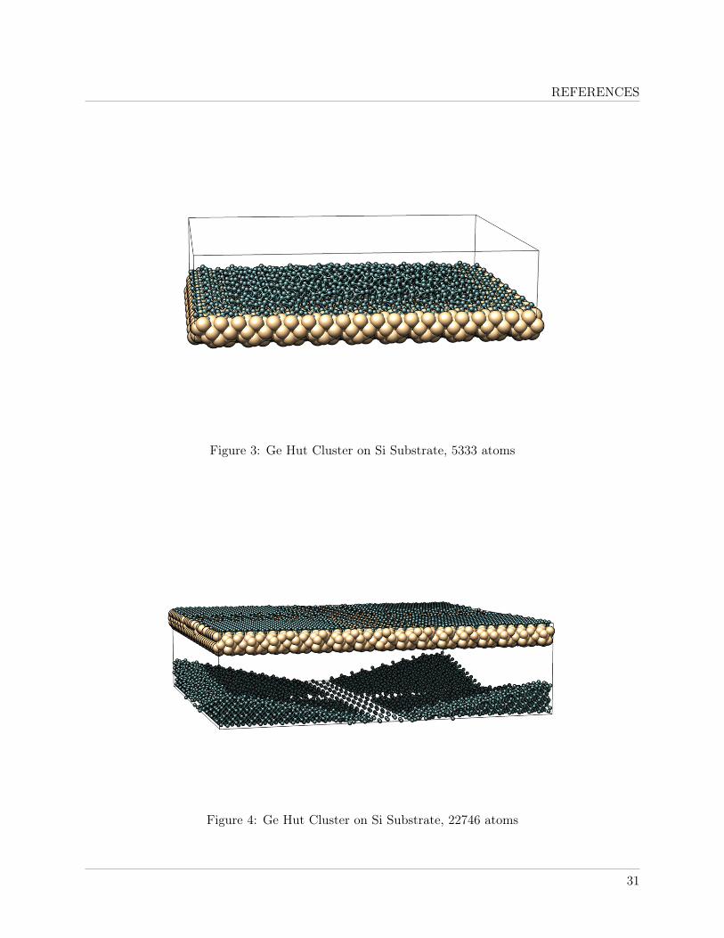
REFERENCES
Figure 3: Ge Hut Cluster on Si Substrate, 5333 atoms
Figure 4: Ge Hut Cluster on Si Substrate, 22746 atoms
31
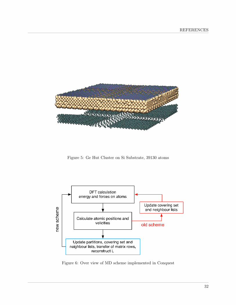
REFERENCES
Figure 5: Ge Hut Cluster on Si Substrate, 39130 atoms
Figure 6: Over view of MD scheme implemented in Conquest
32
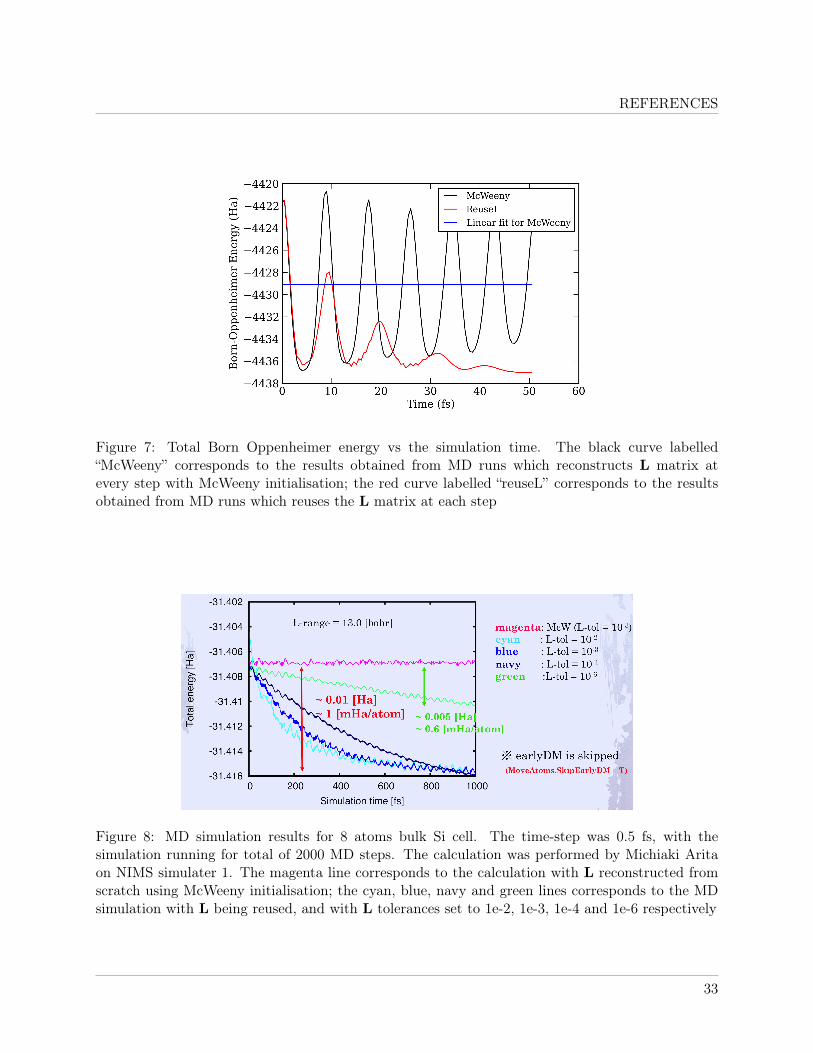
REFERENCES
Figure 7: Total Born Oppenheimer energy vs the simulation time. The black curve labelled“McWeeny” corresponds to the results obtained from MD runs which reconstructs L matrix atevery step with McWeeny initialisation; the red curve labelled “reuseL” corresponds to the resultsobtained from MD runs which reuses the L matrix at each step
Figure 8: MD simulation results for 8 atoms bulk Si cell. The time-step was 0.5 fs, with thesimulation running for total of 2000 MD steps. The calculation was performed by Michiaki Aritaon NIMS simulater 1. The magenta line corresponds to the calculation with L reconstructed fromscratch using McWeeny initialisation; the cyan, blue, navy and green lines corresponds to the MDsimulation with L being reused, and with L tolerances set to 1e-2, 1e-3, 1e-4 and 1e-6 respectively
33

REFERENCES
Figure 9: Total Born Oppenheimer energy vs the simulation time for various L tolerances. The blackcurve labelled “McWeeny” corresponds to the results obtained from MD runs which reconstructs Lmatrix at every step with McWeeny initialisation; The rest of the curves corresponds to the resultsobtained from MD runs which reuses the L matrix at every step, with different L tolerances
34
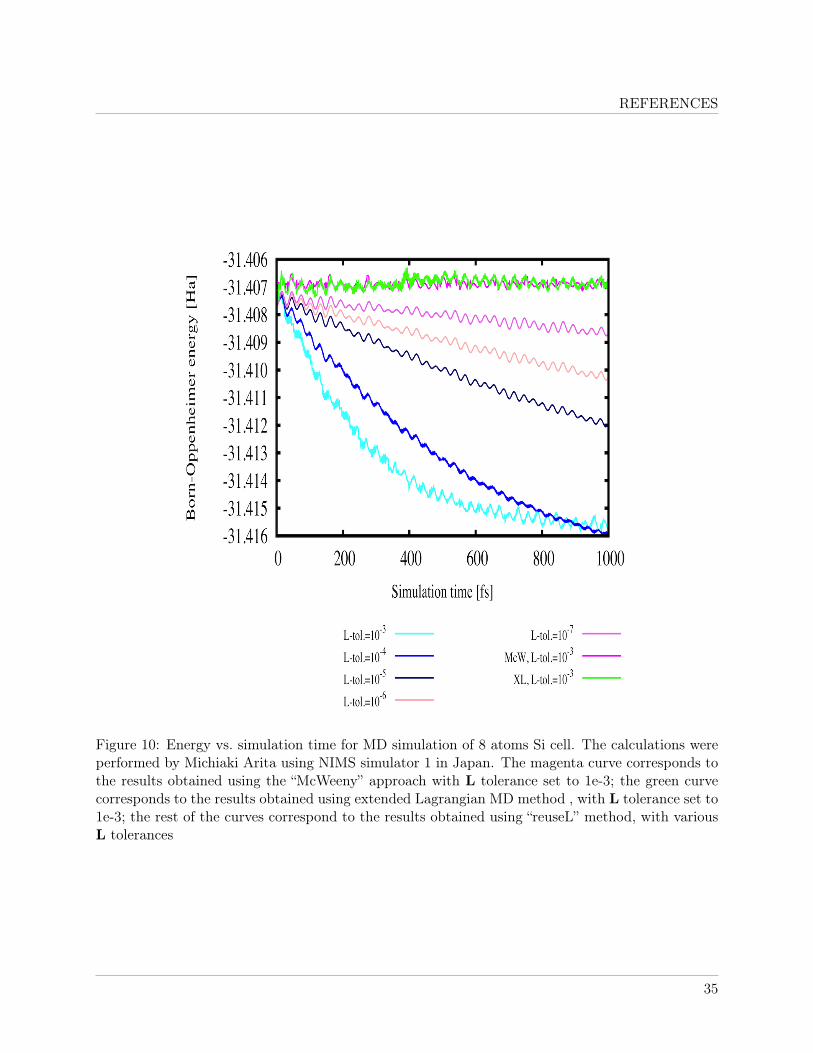
REFERENCES
Figure 10: Energy vs. simulation time for MD simulation of 8 atoms Si cell. The calculations wereperformed by Michiaki Arita using NIMS simulator 1 in Japan. The magenta curve corresponds tothe results obtained using the “McWeeny” approach with L tolerance set to 1e-3; the green curvecorresponds to the results obtained using extended Lagrangian MD method , with L tolerance set to1e-3; the rest of the curves correspond to the results obtained using “reuseL” method, with variousL tolerances
35
Related Documents