Daytime temperature sum — a new thermal variable ...

BOREAL ENVIRONMENT RESEARCH 9: 319–333 ISSN 1239-6095Helsinki 31 August 2004 © 2004

Daytime temperature sum — a new thermal variable describing growing season characteristics and explaining evapotranspiration

Reijo Solantie

Finnish Meteorological Institute, Meteorological Research/Climate Research, P.O. Box 503, FIN-00101 Helsinki, Finland

Solantie, R. 2004: Daytime temperature sum — a new thermal variable describing growing season characteristics and explaining evapotranspiration. Boreal Env. Res. 9: 319–333.

The effective temperature sum, the sum of the positive differences between diurnal mean temperatures and 5 °C, is used in ecology, agriculture, forestry, and hydrology. It does not differentiate between day and night. However, most assimilation and eva-potranspiration occurs in the daytime. A “daytime temperature sum” is presented that is better related to assimilation. First, temperatures above 7 °C were integrated during the period, starting when the sun rises five degrees above the horizon, and ending when it descends to two degrees. The sums of these values were then reduced to be, on average, equal to the traditional ones. The new variable appeared to smooth out much of the spatial variation caused by night-time temperatures. It also gives a more distinct start and end to the thermal vegetation period. When using the daytime temperature sum instead of the traditional sum in explaining evapotranspiration, a better result was obtained.

Introduction

Thermal demands in the development stages of boreal vegetation

The effective temperature sum is a thermal vari-able that is widely used in various climatic applications in the boreal zone. This variable is calculated as routine by all the Nordic Mete-orological, Agricultural and Forestry Institutes. The intensity of assimilation, as measured by the agricultural production of dry substance, is fairly well proportional to the daily increment of the effective temperature sum; further, in north-ern conditions where temperature is a dominant factor, the process of crop development between its consecutive stages corresponds approximately

to constant increments in this variable (Skjelvåg et al. 1992). This variable is also used to calcu-late evapotranspiration in conditions in which the lack of water is not a significant restricting factor (e.g. Hyvärinen et al. 1995, Solantie and Joukola 2001); on the other hand, evapotranspi-ration is well correlated with the growth of forest stands (Solantie 2003), a consequence of assimi-lation. The traditional method of calculating the effective temperature sum in a particular year is to sum the positive differences between the diurnal mean temperatures and 5 °C (in Finland, 6 °C in a few other countries). The correspond-ing climatic means can be calculated either as the mean of such annual values, or by summing the positive differences between 5 °C and the diurnal means over the years considered. The

320 Solantie • BOREAL ENV. RES. Vol. 9

former method gives 30–40 °C d greater values than the latter.

The biotemperature, i.e., the temperature sum above the freezing point, is also used to measure vegetative development (Holdridge 1967). Con-sidering that, even for such a boreal and arctic species as Rubus chamaemorus (cloudberry), the freezing point seems to be too low a temperature for the start of growth, the lower temperature limit with respect to the diurnal mean should be 5 °C, in preference to 0 °C. Additionally, in the inland climates of Fennoscandia, and even more in continental climates, the ground is either snow-covered and/or frozen until about 5 °C. Correspondingly, in autumn, dormancy must be prepared for in good time before the climatic start of thermal winter when temperatures down to –20 °C may occur.

The main fault in the traditional method, how-ever, is that it assumes that each degree above 5 °C has an equal effect without differentiating between day and night or taking into account day length. First, most of the evapotranspiration and practically all the assimilation occurs when the sun is above the horizon. Let us take Rubus chamaemorus (cloudberry) as an example: it has a circumpolar distribution covering all the sub-zones of the boreal main zone (Taylor 1971), and has been comprehensively studied in its various areas of occurrence. Its assimilation increases practically linearly with air temperature (T ) in the range of 8 to 18 °C, but outside this optimal range remains below this linear relationship, and practi-cally ceases below 3 °C and above 25 °C (Kostyt-schew et al. 1930, Lohi 1974, Marks and Taylor 1978, Kortesharju 1982). In fact, temperatures below 3 °C are quite common in the early and late parts of the growing season, as well as tempera-tures below 8 °C in the middle of the summer.

The newest research results regarding the photosynthesis of conifers show that assimila-tion is very tightly regulated both by temperature and light (Mäkelä et al. 2004). It begins to appre-ciably increase immediately after sunrise at solar radiation of 10 W m–2. The start in spring is not very sharp but some increase is already observed slightly before the mean temperature has risen to 5 °C.

Considering agricultural applications, the temperature conditions for the cereals grown

in Finland are rather similar to those for Rubus chamaemorus. As the lower limit of the diur-nal mean temperature, over which the tempera-ture sum best explains the various development stages for barley (the crop species grown farthest north), 2 °C is more appropriate than 5 °C (Lal-lukka et al. 1978). Kleemola (1991), using a non-linear model to explain the development of spring wheat, found that the limit of the diurnal mean temperature on average for three cultivars was 3 °C, both for the development from sowing to heading and from heading to yellow ripen-ing; the upper limit of the optimal temperature range was 22 to 25 °C. Kontturi (1979) found somewhat higher values for the lower mean tem-perature limits for spring wheat: from sowing to heading 4 °C, from heading to ripening 8 °C and from sowing to ripening 6 °C. Further, both day length and global radiation, as well as their com-bined effect with temperature, have proved to be an important factor for the development of crops (Åkerberg and Haider 1976, Lallukka et al. 1978, Major 1980). The effect of both seasonal and latitudinal differences in day length on the devel-opment of crops in Boreal conditions was already discovered in a rather early stage of agricultural research (Eikeland 1936, Robertson 1968). On the other hand, for some crops, the photoperiod in southern Finland seems to be long enough to ensure maximal production in this respect (Saarikko and Carter 1999). Obviously, the skill of the plant in making use of the long days does depend a lot on the species and cultivars, but is obviously best for native vegetation. One pos-sible reason for the controversial result by Saa-rikko and Carter (1999) may be that in eastern Bothnia the soil frost is deeper and the soil cooler in early summer than in southern Finland (more in the discussion).

Why and how to replace a good old method with a new one?

In considering the developmental stages of veg-etation, the use of the traditional method leads to a disagreement between the calculated and actual differences between seasons and regions. Another fault is the fact that the intensity and frequency of nightly inversions considerably influence the

BOREAL ENV. RES. Vol. 9 • Daytime temperature sum 321

traditional effective temperature sum. This leads to a paradox: when improving the resolution in spatial analyses of the mean temperature and traditional effective temperature sum, just those features in the spatial variation that are caused by the spatial variations of nightly surface inver-sions, and are nonessential, appear most promi-nent. This “improvement”, in fact, worsens the effective temperature sum’s ability to explain the spatial variation in assimilation, development of vegetation, and evapotranspiration than earlier, coarser and therefore smoother analyses of the effective temperature sum. On the basis of the discussion above, a general method for various purposes can be found with satisfactory accu-racy. It is, therefore, the proper time to create a tool to calculate the main thermal variable, also taking into account the day length, and to apply this to the various climatic applications in agri-culture, forestry, ecology and hydrology.

The “daytime temperature sum”, according to the foregoing, was developed and experi-mented with. A comparison between the “tradi-tional” and “new” methods was also made. For this purpose, a map of the “daytime temperature sum” 1961–1990 was calculated in 10 ¥ 10 km grid-squares; such a map of the traditional tem-perature sum is already available (Solantie and Drebs 2000). To be comparable with the “tradi-tional” values, the new ones had to be multiplied by the relation of the “traditional” and “new” averages over the whole of Finland; the inverse of this relation is practically equal to the daytime period (h) averaged over the vegetation period and over Finland, and divided by 24 h. This attempt is meant to be a starting point for more sophisticated versions, taking into account spe-cies-specific thermal demands.

Development of daytime temperature sum: theoretical background and methods

Lower limits for radiation and temperature

In calculating the new thermal variable, the night-time was excluded. In the morning, assimi-lation is determined practically by air tempera-

ture, after global radiation has attained a certain limit (which, according to Marks and Taylor (1978), is 60 W m–2 for Rubus chamaemorus). According to observations at Luonetjärvi in Cen-tral Finland in the summer months of 1981–1990 (Finnish Meteorological Institute 1993), this value was, on average, reached in the morning when the sun was six degrees above the horizon. At a solar altitude of five degrees, about 15 min-utes earlier, assimilation is already proceeding well, and this may be considered as an appropri-ate end to night-time. On the other hand, even smaller angles are less appropriate because in the morning, e.g. at a solar altitude of two degrees, the temperature is still near the night minimum, and quite often below the optimal range. In the evening, assimilation and “daytime” obviously continue somewhat longer because of continuity and higher temperature; consequently, a solar altitude of two degrees may be more appropriate for the end of daytime.

Using these limits for solar altitude, and setting the lower limit for the new daytime mean as 7 °C instead of 5 °C for the originally-used diurnal mean, the thermal vegetation period begins and ends approximately contemporarily with the corresponding period calculated tradi-tionally. The daily contribution to the daytime temperature sum can thus be expressed as d(Td – 7 °C), where d is the proportion of the included period, i.e., the “daytime”, of 24 hours, and Td is the mean daytime temperature during the period 1961–1990. The daily contribution is thus accepted only if Td > 7 °C. When Td = 7 °C, the average temperature in the morning for a solar altitude of five degrees is 1 °C in spring and 3 °C in autumn. At the beginning of the veg-etation period, the crucial limit of 3 °C is in fact achieved an hour later than the five degrees solar altitude, but already ten days later this value is attained simultaneously with the five degrees solar altitude.

Daytime temperature sum as a function of day length and diurnal temperature amplitude

The differences in local features between the “daytime” (new) and “traditional” temperature


sums in spatial analyses are mainly caused by the day length and the diurnal temperature ampli-tude. To understand this, we begin with the fact that the mean temperature during assimilation hours, Td, can be given as

Td = T + (1 – d)(Td – Tn) (1)

where T is the diurnal mean temperature, Tn is the mean temperature outside the daytime period, and d is the ratio of the daytime portion to the whole 24 hours.

On the basis of observational material for various calendar days during the vegetation period, and various climatic zones in Finland, we can make the approximation that

(Td – Tn) = aA (2)

where a is an empirical coefficient, having a value of 0.48 (see next section), and A is the diurnal temperature amplitude. Thus we obtain

Td = T + 0.48(1 – d)A (3)and Ld = d(T + 0.48(1 – d)A – 7) (4)

where Ld is the daily contribution to the daytime temperature sum.

Further, the daily climatic mean values of the daytime temperature sum are calibrated during the vegetation period, so that on average in Fin-land

∑Ldd = ∑L = k ¥ ∑Ld, (5)

where ∑Ld is the sum of Ld (Eq. 4) over the vegetation period, k = calibrating factor, approxi-mately the inverse of the average value of d, having a value of 1.56, and ∑L is the average traditional effective temperature sum.

The precise value of k was obtained by divid-ing the value of L, averaged over the whole of Finland and the period 1961–1990 by the cor-responding value of Ld. It turned out to be 1.56, i.e., equal to the provisional value. Through this calibration, the possible inaccuracy in the value of the coefficient a for the period 1961–1990 did not disturb the comparison between either method, as reported in the next section. Applying

the value of k to the daily contributions of day-time temperature we have

Ldd = 1.56(Td – 7) (6)or Ldd = 1.56d(T – 7) + 0.75 (d – d 2)A (7a)

If adequate amounts of observations of con-tinual registration are available, the values of Td can be directly calculated from observations; however, the latitude and longitude of the station and the calendar day are needed as basic data to obtain any individual diurnal value of Ldd. How-ever, Eq. 7a is an easy way to obtain values of Ldd for stations without continual observations. We may even approximate T as the weighted mean of diurnal maxima and minima, so that these are the only indispensable temperature observations needed to obtain the daytime tem-perature sum.

Magnitude of the coefficient a

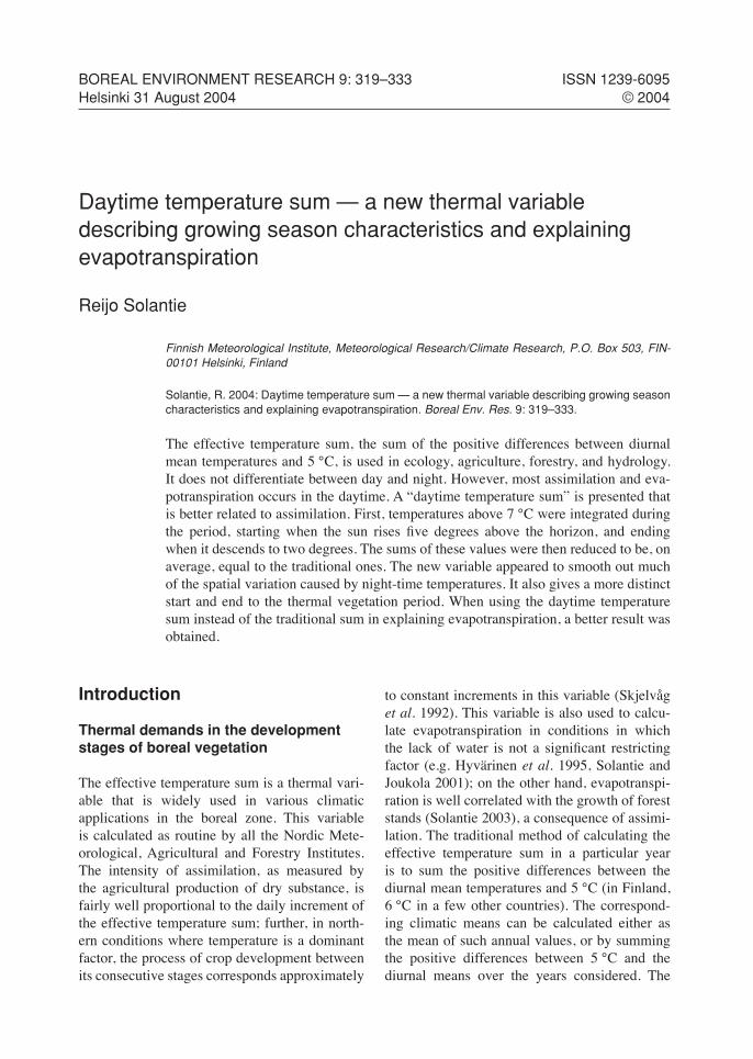
The behaviour of coefficient a, giving (Td – Tn)/A, depends somewhat on the prevailing weather conditions and also slightly on land-type. There-fore, in applications for single days and months, a study of the accuracy of a and the sensitiv-ity of Ldd to it is needed (while this was not so important in the calculation of the 1961–1990 means, because the mean level of the results was calibrated to be equal to that of L). To obtain the magnitude of a in various weather condi-tions and land-types, the basic material used was the temperatures continuously registered in the Möksy experimental field in 2002 (Fig. 1). From 19 June of that year, six Hobo thermometers were situated in Möksy in various terrains.

In the inland climate of northern Europe, precipitation mostly falls in summer as day-time showers, while nights are often clear. The daytime temperature thus varies a lot between the showers and the sunny intervals, so that Td remains more below the daily maximum than during clear days with rather regular tempera-tures. For this reason, the value during cool and rainy summers is lower than in warm and sunny summers such as 2002. Also, during the observa-tion period at Möksy following 19 June 2002,


70°N

65°N

20°E 30°E

60°N

100 kmHB

SB

MB

NB

Fig. 1. The locations of the Möksy experimental field () within the middle boreal zone (MB) and Kuopio airport (Siilinjärvi) () within the southern boreal zone (SB). Also shown are: HB = hemibo-real zone, NB = northern boreal zone, and Lake-Finland (part of the SB north of the dotted line).

we may distinguish between the bright and hot period lasting through July and August and the cooler and more unstable periods of 19–30 June and 1–30 September. During the period 1 July–31 August, the weighted mean of a was 0.52 for peatlands and 0.49 for mineral soils, while the corresponding values in June were 0.45 and 0.42, and in September 0.45 and 0.39.

The mean values of a during the period 19

June–30 September on the four peatland sites were 0.49 to 0.51, and on the mineral soil sites 0.48 (open sitation) and 0.46 (pine stands). The weighted mean for peatland sites was 0.50 and for mineral soil sites 0.46; the weights corre-spond to the actual land-type distribution in the middle boreal zone (Fig. 1). In order to calculate the mean daytime temperature sums for the period 1961–1990, a was approximated by 0.48,


in accordance with some series of Milos obser-vations from the southern boreal zone during the period 2000–2002 (Fig. 1).

Additional basic material is given by Heino (1973). He studied diurnal temperature variation by analysing the registrations on thermogram charts during the unusual cold period 1956–1965. Calculating the values of a from six main-land stations having observations over 10 years, the northernmost being Sodankylä observatory (62°22´N), values of 0.41 to 0.44 were found, with an average of 0.42. All in all, 0.45 seems to be the most appropriate value for general purposes, corresponding to average weather and soil conditions. In order to counterbalance the effect of replacing a = 0.48 by a = 0.45 on the all-over average of Ldd so as to keep it equal to the all-over average of L, Eq. 7a would have to be replaced by Eq. 7b:

Ldd = 1.59d(T – 7) + 0.71(d – d 2)A (7b).

In most cases, the value of a falls within the limits 0.45 ± 0.03, and only in extreme cases outside the limits 0.45 ± 0.06. With the former limits, the use of the value of 0.45 causes errors of ±0.17 °C in Td and errors of ±25 to ±30 °C d in the daytime temperature sum over the veg-etation period. The corresponding errors in the case of the latter limits for a are correspondingly ±0.35 °C and ±50 to ±60 °C d. This error is only 5% of the climatic mean, or 25% of the mean difference between the averages in the southern boreal (denoted by SB) and middle boreal (MB) zones, or between the averages in the middle boreal and northern boreal (NB) zones (Fig. 1).

Difference between the traditional and daytime temperature sums

Referrring to Eq. 7a, the difference between the new and the traditional daily values is

Ldd – L = (1.56d – 1)T + (5 – d10.92) + 0.75(d – d 2)A (8)

By grouping the daily contributions so as to consist of two terms (in the outer parentheses), we obtain

Ldd – L = [0.75(d – d 2)A + d(1.56T – 10.92)] + (– T + 5) (9)

Creating maps

In creating a map of the average daytime tem-perature sum 1961–1990, the gridded values of mean minimum and maximum temperatures for the period 1 May–30 September 1961–1990 (Solantie and Drebs 2000) were used as basic material; the grid size is 10 ¥ 10 km.

The mean temperature T for the period 1 May–30 September was obtained as a weighted mean of the mean diurnal minimum and maxi-mum; the empirical weight of the maximum is

Wmax = 0.37 + 0.025Ameandmean (10)

where Wmax is the weight of the maximum, while Amean and dmean are the mean of the diurnal ampli-tude and the ratio of the daytime to the whole 24 hours over the days of the vegetation period and over climatic zones, respectively. Approximately, Wmax has a value of 0.515 for the NB, 0.55 for the MB, and 0.53 for the SB.

By applying Eq. 7a for calculating the day-time temperature sum for the period May–Sep-tember, the values of the involved variables aver-aged over the whole period were used instead of the sum of daily results. This causes a small correction D∑Ld, given by

D∑Ld = 20 + 2 (latitude – 60) (11)

A small correction is also needed to precisely adjust the daytime temperature sum for the five-month period considered to the exact thermal vegetation period. In central Finland the veg-etation period begins, on average, on 1–5 May and ends around the end of September. Farther north, it begins later in May, while farther south an increment must be added in October. These small adjustments were also made as a function of the number of days to be included in the veg-etation period with the criterion Td > 7 °C at the beginning and end of the months of this period (N ), and the rising/falling rate of Td (°C per day) at the end of the vegetation period (rate). The monthly increment is thus 0.5N rate. Further, the


mean of d for the whole vegetation period can be approximated as

dmean = 0.62 + 0.0011(latitude – 60) (12)

The application is thus simple, and random irregularities are avoided.

Results

Analytical comparison between the traditional and daytime temperature sums

By considering Eq. 9, it was found that the dif-ferences between the daily contributions to the daytime temperature sum and to the traditional one can be given as the sum of two components, one being a function of the diurnal temperature amplitude and day length, and the other a func-

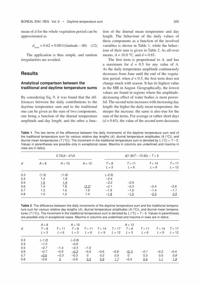
tion of the diurnal mean temperature and day length. The behaviour of the daily values of these components as a function of the involved variables is shown in Table 1, while the behav-iour of their sum is given in Table 2. As all-over means, A = 10.0 °C, and d = 0.65.

The first term is proportional to A, and has a maximum for d = 0.5 for any value of A. As the daily temperature amplitude continuously decreases from June until the end of the vegeta-tion period, when d ≈ 0.5, the first term does not change much with season. It has its highest value in the MB in August. Geographically, the lowest values are found in regions where the amplitude-decreasing effect of water bodies is most power-ful. The second term increases with increasing day length: the higher the daily mean temperature, the steeper the increase; the same is also true for the sum of the terms. For average or rather short days (d < 0.65), the value of the second term decreases

Table 1. The two terms of the difference between the daily increments of the daytime temperature sum and of the traditional temperature sum for various relative day lengths (d ), diurnal temperature amplitudes (A (°C)), and diurnal mean temperatures (T (°C)). The increment in the traditional temperature sum is denoted by L (°C) = T – 5. Values in parentheses are possible only in exceptional cases. Maxima in columns are underlined and maxima in rows are in italics.

0.75(d – d 2)A d(1.56T – 10.92) – T + 5

d A = 8 A = 10 A = 12 T = 8 T = 11 T = 14 T = 17 L = 3 L = 6 L = 9 L = 12

0.3 (1.3) (1.6) (–2.5)0.4 1.4 1.8 –2.40.5 1.5 1.9 –2.2 –2.90.6 1.4 1.8 (2.2) –2.1 –2.3 –2.4 –2.60.7 1.3 1.6 1.9 –1.9 –1.6 –1.4 –1.10.8 1.0 1.2 1.4 –1.8 –1.0 –0.3 0.5

Table 2. The difference between the daily increments of the daytime temperature sum and the traditional tempera-ture sum for various relative day lengths (d ), diurnal temperature amplitudes (A (°C)), and diurnal mean tempera-tures (T (°C)). The increment in the traditional temperature sum is denoted by L (°C) = T – 5. Values in parentheses are possible only in exceptional cases. Maxima in columns are underlined and maxima in rows are in italics.

A = 8 A = 10 A = 12d T = 8 T = 11 T = 8 T = 11 T = 14 T = 17 T = 8 T = 11 T = 14 T = 17 L = 3 L = 6 L = 3 L = 6 L = 9 L = 12 L = 3 L = 6 L = 9 L = 12

0.3 (–1.2) (–0.9)0.4 –1.0 –0.60.5 –0.7 –1.4 –0.3 –1.00.6 –0.7 –0.9 –0.3 –0.5 –0.6 –0.8 (0.1) –0.1 –0.2 –0.40.7 –0.6 –0.3 –0.3 0 0.2 0.5 0 0.3 0.5 0.80.8 –0.8 0 –0.6 0.2 0.9 1.7 –0.4 0.4 1.1 1.9


slightly with increasing mean temperature (T ), while for longer days (d > 0.65) it increases with increasing T, as does also the summed term. In all cases, the summed term increases with increasing amplitude, at a rate of 0.1–0.2 °C d per °C of T. Because a combination of long day, high mean temperature, and large diurnal amplitude max-imises the value of the summed term, the highest mean daily values (0.5 °C d or more) in the SB occur in June, in the MB in June and July, and in the NB in July (Fig. 1). As the diurnal amplitude is greater in the MB than in either the SB or the NB, and that there the day is longer than in the SB, and the summer is warmer than in the NB, it is clear that the summed term is greater in the MB than in either the SB or the NB (the daily mean values being 0.7–0.9 °C d in both June and July). Negative values occur during the first 30 days of the vegetation period, and after late July (first in Lake-Finland (Fig. 1)) or early August (latest in the NB). The lowest values, –1.1 to –1.4 °C d are found in September and early October in Lake-Finland, where the amplitude is smallest due to the season and the effect of water bodies, and where T in that season is appreciably higher than in other inland regions; as noted before, in the case of short days (d < 0.65), the second term decreases with increasing T. This ensures the appropriate start of hibernation, despite warm periods in late autumn. Note also that in the light conditions of early summer, the daytime tem-perature is very sensitive to changes in T, which means that assimilation is cautious while a high risk of heavy frosts is present. In accordance with this, as long as the mean temperature is still below 10 °C, the difference between the “new” and “tra-ditional” results for northern-Finnish day-length conditions is negative, and lower than in southern Finland for the same diurnal amplitudes.

There are two main reasons for the differences between the results given by the two methods. First, the day increases in length northwards, caus-ing the new method to give smaller north-south gradients. The second is the omission of the night-time period, which causes larger values in regions with steep night-time surface inversions, such as the MB, and also causes smaller values in regions where the nights are heated, e.g., by water bodies, by above-inversion situations on hill sides, and by tall forest stands. When using the traditional

method, the great spatial variation in night temper-atures, in particular, causes strong random irregu-larities in the spatial field; this difficulty is avoided by using the new method. The steep gradient across the boundary between the SB and MB, being according to the traditional method 60 °C d, is appreciably smaller (about 20 °C d) according to the new method. The differences between the MB and NB, however, are slightly greater by the new method than by the traditional; this is caused by the fact that the diurnal amplitude in the MB is appreciably greater than in the NB.

We may also note that when comparing the values of growth intensity for equal diurnal mean temperatures in May and late summer with each other, both methods give equal values, while the new method gives greater values in June and July. So, the role of the mid-summer is thus more important and the role of late summer is less important when compared to the tradi-tional method. Additionally, as both the duration of the daytime and the value of Td – T decrease steeply with time in autumn, the growing season, determined according to the daytime temperature sum, ends more distinctly than when calculated traditionally.

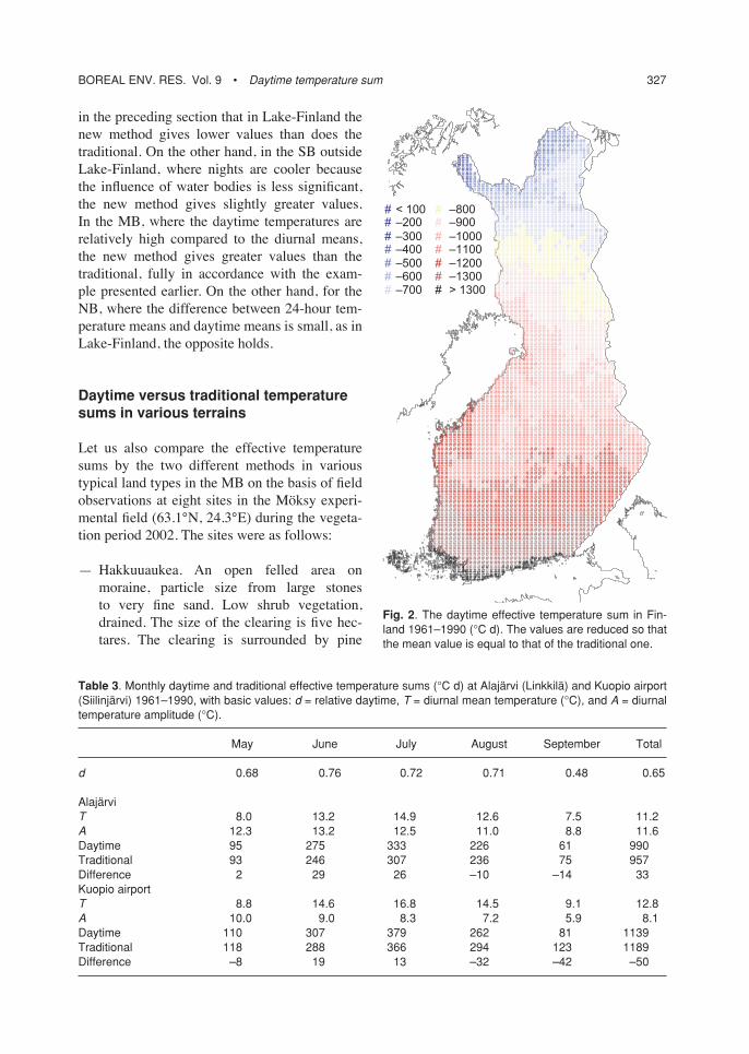
An example (Table 3) is given of the mean monthly sums of the effective temperature 1961–1990 according to the daytime method (Eq. 7a) and the traditional one for two stations at the latitude 63 °N, Alajärvi (Linkkilä) in the MB within the Möksy experimental field (Fig. 1), and Kuopio airport (Siilinjärvi) within the north-ern Lake-Finland region of the SB. This example with two sites, representative of their regions, shows that in the MB the new method gives higher values than the traditional while the oppo-site holds for Lake-Finland where nights are warm due to the influence of water bodies.

A map for the daytime temperature sum and another map for the difference between the daytime and traditional temperature sums

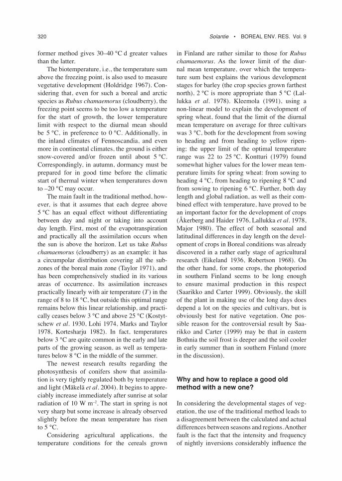
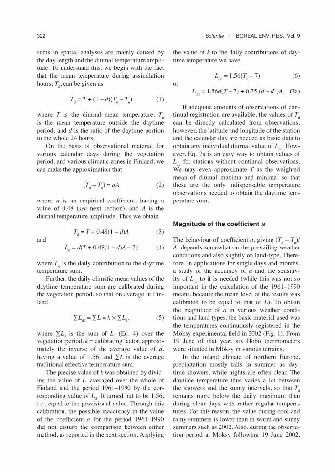
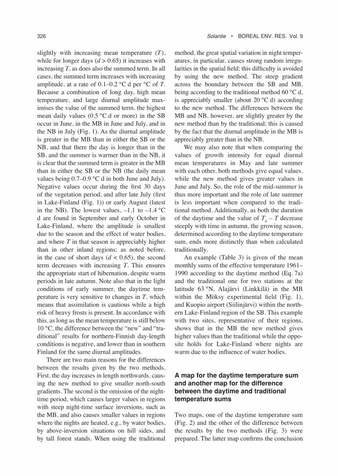
Two maps, one of the daytime temperature sum (Fig. 2) and the other of the difference between the results by the two methods (Fig. 3) were prepared. The latter map confirms the conclusion


in the preceding section that in Lake-Finland the new method gives lower values than does the traditional. On the other hand, in the SB outside Lake-Finland, where nights are cooler because the influence of water bodies is less significant, the new method gives slightly greater values. In the MB, where the daytime temperatures are relatively high compared to the diurnal means, the new method gives greater values than the traditional, fully in accordance with the exam-ple presented earlier. On the other hand, for the NB, where the difference between 24-hour tem-perature means and daytime means is small, as in Lake-Finland, the opposite holds.

Daytime versus traditional temperature sums in various terrains

Let us also compare the effective temperature sums by the two different methods in various typical land types in the MB on the basis of field observations at eight sites in the Möksy experi-mental field (63.1°N, 24.3°E) during the vegeta-tion period 2002. The sites were as follows:

— Hakkuuaukea. An open felled area on moraine, particle size from large stones to very fine sand. Low shrub vegetation, drained. The size of the clearing is five hec-tares. The clearing is surrounded by pine

Table 3. Monthly daytime and traditional effective temperature sums (°C d) at Alajärvi (Linkkilä) and Kuopio airport (Siilinjärvi) 1961–1990, with basic values: d = relative daytime, T = diurnal mean temperature (°C), and A = diurnal temperature amplitude (°C).

May June July August September Total

d 0.68 0.76 0.72 0.71 0.48 0.65

Alajärvi T 8.0 13.2 14.9 12.6 7.5 11.2A 12.3 13.2 12.5 11.0 8.8 11.6Daytime 95 275 333 226 61 990Traditional 93 246 307 236 75 957Difference 2 29 26 –10 –14 33Kuopio airport T 8.8 14.6 16.8 14.5 9.1 12.8A 10.0 9.0 8.3 7.2 5.9 8.1Daytime 110 307 379 262 81 1139Traditional 118 288 366 294 123 1189Difference –8 19 13 –32 –42 –50

#

#####

#####

####

#####

######

#####

######

#######

###

######

####

######

####

#####

######

###

###

###

#

##

##

#####

### #

##

##

## #

##

##

########

########

########

####

### #

##

##

#####

######

#######

######

###

###

###

##

##

##

###

######

#

##############

###############

#################

############

#

########

######

###

##

###

#

#########

############

############

#

#

##

########

######

#############

############

############

########

#

##

###

###

###

### #

##

#####

#######

######

##

###

#####

######

#####

####

#####

###

###

#####

########

##########

#######

#

# ##

#####

####

###

######

####

#

# # ##

####

###

### #

# #

#

##

#####

######

####

##

###

####

#######

#######

#####

###

###

###

#

#######

#######

#

#

####

#####

#####

###

#

##

##

##

###

## #

#

#####

######

########

#######

#####

####

###

####

####

##

# ##

###

#

###

#####

#######

#############

###############

#################

##################

#################

################

#

###############

############

#########

#######

#

##

#

# ###

#

#

####

####

######

#######

########

######

##

####

###

#

##

##

###

######

#########

#############

##############

#############

############

##

######

####

#

#

##########

###########

#

############

############

##########

#########

#########

#

###

###

######

######

######

####

##

####

####

###

###

###

####

###

######

#######

########

########

#####

##

# ###

#####

##

###############

###

###############

#

#######

#

##

##

#############

################

################

################

################

###############

##############

################

###############

################

#

###############

#############

###########

###########

#############

##

#

#

####

######

########

######

###########

#############

################

###

##

#########

########

#######

########

#######

######

########

#

#

####

####

#####

########

########

########

#########

##########

#########

#########

###

###

##

###

######

########

#########

#######

####

##

#

########

#########

########

#######

#####

##

####

####

####

###

#####

######

######

######

#####

###

#

#

###

##

######

########

##########

#########

#####

###

##

##

#####

########

#######

####

##

###

##

######

### #

#

####

#####

###########

#######

##

#######

###

######

##

######

###

####

###

##

####

###

####

##

####

##

####

#

####

####

#

##

###

####

#

#

######

#########

#

#########

#

########

#########

####

# ###

##

###

##

#######

#####

#####

###

##

######

#######

########

#########

#########

####

###

###

###

#

###

##

###

####

###

##

##

#

#######

####

###

###

####

####

#####

#####

####

#####

######

#####

## #

#####

####

####

####

##########

##########

##########

#########

######

##

##

#

####

#####

######

######

######

#####

#####

######

###

##

##

#

######

#######

########

########

###

##

###

####

#####

#####

#####

## #

####

#####

######

########

########

#######

######

####

##

###

#####

######

########

########

########

########

########

##########

#####

##

#

##

#

#

#

#

#####

######

######

######

######

####

###

##

##

###

#####

#####

######

#####

#

#######

#######

######

#####

#####

#####

####

#####

#####

#####

#####

####

####

###

###

##

##

###

####

###

###

##

##

##

#####

##

#####

####

#####

#########

########

######

#########

###########

############

############

#######

####

###

###

#

#

###

###

###

##########

###########

###########

############

################

####################

#####################

####################

######

##

##########

#####

###########

##

###########

#

####

###

###

##

##

#######

#########

##########

#############

###

##########

#######

#####

#

###

#####

#######

############

#################

#################

###############

################

#####

########

###

#########

#####

#

###

###

####

## #

###

#

####

#########

########

######

##

##

###

#####

######

######

#####

###

###

##

#

##

#####

######

#######

########

###########

#############

#############

############

#############

#############

##########

##########

#########

########

#########

##

#

## # #

# ## ##

##

## # #

# < 100# –200# –300# –400# –500# –600# –700

# –800# –900# –1000# –1100# –1200# –1300# > 1300

#

Fig. 2. The daytime effective temperature sum in Fin-land 1961–1990 (°C d). The values are reduced so that the mean value is equal to that of the traditional one.


forest on mineral soil of the same kind.— Koreakangas. Pine forest. Soil as at the

Hakkuuaukea site. Low shrub vegetation.— Muuttuma. Mixed forest, mainly Scots pine,

with scattered birches and spruces. Forest grown on a drained bog.

— Kompassiräme. A drained bog with sparse and low pine stands, afforestation unsuccess-ful. Low shrub vegetation. Thick Spaghnum moss peat. Drained. Surrounded by bogs with successful drainage and taller pine stands.

— Reunaräme. A bog in a natural state, growing

low and sparse pine stands. Shrubs of aver-age height, Spaghnum moss.

— Pohjoisneva. A fen in a natural state. Single groups of small pines and sedge vegetation on hummocks. Hollows lacking vegetation, filled by shallow water except for dry periods in summer.

— Linkkilä, having a Milos thermometer with continuous registration and up-to-date mes-saging. The station is located in a field sur-rounded by forest grown on drained mires. The clearing consists mainly of lawns, and next to the screen there is a small field grow-ing strawberries and potatoes.

— Huosianmaa. A standard climatic station, thus recording temperatures at 6, 12, 18 and 24 UTC (the last one read from the thermo-graph record), and minimum and maximum temperatures for each 12-hour period, daily precipitation, state of ground, extent of snow cover, and snow depth. Situated on a hill. Cultivated field, growing mainly grass. The inorganic material of the soil is glacial till, comprising many fine particles.

The differences in effective temperature sums, obtained by the same methods at different sites, are given as percentages of the deviations of values at the sites from their weighted mean. Relative values are used because observations there did not begin until 19 June, so that the whole of the vegetational period could not be measured. As the climatic long-period means of the effective temperature sum in the MB are very close to 1000 °C d, such relative deviations and differences, multiplied by 10, give absolute deviations in °C d. All values could be calculated directly from continuous observations without any approximations.

According to the traditional method, hill sides are extremely advantageous places (excess 7%), clearings on mineral soils appreciably advanta-geous (excess 4%), and pine stands on mineral soils rather advantageous (excess 1.5%). Virgin fens, virgin bogs and the Linkkilä site are aver-age (deviations 0.6 to –0.7%). On the other hand, drained bogs, both those with unsuccessful drainage and those having pine stands after suc-cessful drainage, are more disadvantageous than average (deficit –2%).

#

#####

#####

####

#####

######

#####

######

#######

###

######

####

######

####

#####

######

###

###

###

#

##

##

#####

### #

##

##

## #

##

##

########

########

########

####

### #

##

##

#####

######

#######

######

###

###

###

##

##

##

###

######

#

##############

###############

#################

############

#

########

######

###

##

###

#

#########

############

############

#

#

##

########

######

##############

############

############

########

#

##

###

###

###

### #

##

#####

#######

######

##

###

#####

######

#####

####

#####

###

###

#####

########

##########

#######

#

# ##

#####

####

###

######

####

#

# # ##

####

###

### #

# #

#

##

#####

######

####

##

###

####

#######

#######

#####

###

###

###

#

#######

#######

#

#

####

#####

#####

###

#

##

##

##

###

## #

#

#####

######

########

#######

#####

####

###

####

####

##

# ##

###

#

###

#####

#######

#############

###############

#################

##################

#################

################

#

###############

############

#########

#######

#

##

#

# ###

#

#

####

####

######

#######

########

######

##

####

###

#

##

##

###

######

#########

#############

##############

#############

############

##

######

####

#

#

##########

###########

#

############

############

##########

#########

#########

#

###

###

######

######

######

####

##

####

####

###

###

###

####

###

######

#######

########

########

#####

##

# ###

#####

##

###############

###

###############

#

#######

#

##

##

#############

################

################

################

################

###############

##############

################

###############

################

#

###############

#############

###########

###########

#############

##

#

#

####

######

########

######

###########

#############

################

###

##

#########

########

#######

########

#######

######

########

#

#

####

####

#####

########

########

########

#########

##########

#########

#########

###

###

##

###

######

########

#########

#######

####

##

#

########

#########

########

#######

#####

##

####

####

####

###

#####

######

######

######

#####

###

#

#

###

##

######

########

##########

#########

#####

###

##

##

#####

########

#######

####

##

###

##

######

### #

#

####

#####

###########

#######

##

#######

###

######

##

######

###

####

###

##

####

###

####

##

####

##

####

#

####

####

#

##

###

####

#

#

######

#########

#

#########

#

########

#########

####

# ###

##

###

##

#######

#####

#####

###

##

######

#######

########

#########

#########

####

###

###

###

#

###

##

###

####

###

##

##

#

#######

####

###

###

####

####

#####

#####

####

#####

######

#####

## #

#####

####

####

####

##########

##########

##########

#########

######

##

##

#

####

#####

######

######

######

#####

#####

######

###

##

##

#

######

#######

########

########

###

##

###

####

#####

#####

#####

## #

####

#####

######

########

########

#######

######

####

##

###

#####

######

########

########

########

########

########

##########

#####

##

#

##

#

#

#

#

#####

######

######

######

######

####

###

##

##

###

#####

#####

######

#####

#

#######

#######

######

#####

#####

#####

####

#####

#####

#####

#####

####

####

###

###

##

##

###

####

###

###

##

##

##

#####

##

#####

####

#####

#########

########

######

#########

###########

############

############

#######

####

###

###

#

#

###

###

###

##########

###########

###########

############

################

####################

#####################

####################

######

##

##########

#####

###########

##

###########

#

####

###

###

##

##

#######

#########

##########

#############

###

##########

#######

#####

#

###

#####

#######

############

#################

#################

###############

################

#####

########

###

#########

#####

#

###

###

####

## #

###

#

####

#########

########

######

##

##

###

#####

######

######

#####

###

###

##

#

##

#####

######

#######

########

###########

#############

#############

############

#############

#############

##########

##########

#########

########

#########

##

#

## # #

# ## ##

##

## # #

# –230 to –190 # –190 to –170 # –170 to –150# –150 to –130# –130 to –110# –110 to –90# –90 to –70

# –70 to –50# –50 to –30# –30 to –10# –10 to 10# 10 to 30# 30 to 50# 50 to 70

Fig. 3. The difference between the daytime and tradi-tional effective temperature sums 1961–1990) (°C d)


According to the new method, unsuccess-ful drainage sites, virgin bogs and hillsides are advantageous places (excess 2%–3%, albeit only a few species tolerate hard frost nights, occurring at any time of summer on the unsuccessful drain-age sites). Virgin fens, clearings in forests and the Linkkilä site are slightly advantageous places (excess 1.1%–1.4%), while forest stands grown on drained bogs are average, and those on min-eral soils are disadvantageous (deficit –2%).

The differences between the results obtained using the two different methods are given as the differences between the percentages given above. According to this comparison, all kinds of peatlands undergo enhancement in their effective temperature sum when the traditional method is replaced by the new one, the change for unsuc-cessful drainage sites being 6%, for virgin bogs 3%, for forest stands grown on drained bogs as well as for Linkkilä surrounded by such terrain 2%, and for fens 1%. On the other hand, Huo-sianmaa, a field on a hill-side, pine stands on mineral soil, and clearings on mineral soil show reduction, the changes being –5%, –4%, and –3%, respectively. Considering that peatlands are appreciably more common in the MB than in the SB, the steep gradient occurring across the boundary between these zones (Solantie 1990) only exists when the parameter is calculated according to the traditional method. We also note that the traditional method exaggerates the dif-ference in the speed of seasonal development of plant species between the SB and the MB, which means that the traditional degree days require-ment for any stage in the MB is lower than in the SB; the corresponding requirements in daytime degree days are equal.

The local variation among the eight sta-tions, in terms of standard deviation, was 3.3% according to the traditional method, but only 1.8% according to the new method. The respec-tive total range of variation using the traditional method was 9.3%, while that given by the new method was 5.5%. According to the new method, all of the most common land types were rather similar. Consequently, it also seems as if the traditional method both exaggerates variations in the temperature conditions for growth and gives erroneous spatial differences; botanical studies on this subject would be desirable.

Daytime temperature sum explaining evapotransporation

In this particular study, the daytime temperature sums for 1961–1990 were averaged for basins for which Hyvärinen et al. (1995), and Solantie and Joukola (2001) calculated traditional effective temperature sums as averages for 1961–1990, and used those, in addition to some other vari-ables, to explain basin values of evapotranspira-tion obtained from the water balance equation. In this study, both regressions were recalculated by replacing the traditional temperature sums with the corresponding daytime temperature sums. Also, differing from the earlier method of Solan-tie and Joukola, the lake evaporation variable was now the same as that used by Hyvärinen et al. (1995). Let us denote the earlier analysis by “traditional”, and the corresponding new version by “daytime”. Two sets of data have been used. Set A contains all the data, while in set B data from the Kivijärvi basin, which had the greatest error of explanation by both traditional and day-time methods (set B), have been excluded.

The evapotranspiration on the total area (E ), is given as

E = (1 – J)(CoL + ∑(CiVi)) + JCJ lakes + intercept (13)

where J is the proportion of lakes in the area, Co is the coefficient of the effective temperature sum L, Ci are the coefficients of the variables (Vi) “trees” (i = 1), “drought” (i = 2) and ‘fens’ (i = 3), and CJ = the coefficient for the variable “lakes” (Table 4). Here “trees” is the volume of growing forest stands (m3 ha–1 of total land area), “drought” is a function of the difference between evapotranspiration and precipitation and the occurrence of heavily-wooded forests, “fens” is the fens percentage of the total land area, and “lakes” is the sum of the terms v(es – ea) over open water, in which es is the condensation vapour pressure at the surface water temperature, ea is vapour pressure in the air at the two-meter level and v is the wind speed over lakes at the two-meter level.

It should be noted that the drought index = 0, except in grid squares where the mean eva-potranspiration in July in treeless places also


exceeds precipitation and where there are heav-ily-wooded forests whose mean volume of grow-ing stands exceeds 200 m3 ha–1. In such grid squares, the drought index itself is positive but its coefficient is negative.

Concerning the great error of explanation for the Kivijärvi basin, the obvious reason is that there are no precipitation or snow measurements on the high areas near the watersheds but only in the large lake valleys, so that the precipitation and evapotranspiration obtained from the water balance equation are appreciably too low, which is shown by short-period snow and precipitation measurements.

The multiple correlation coefficients obtained using the two methods and two data sets were as follows: in traditional set A 0.975, in traditional set B 0.979, in daytime set A 0.980 and in day-time set B 0.984. The proportions of explained

variance (adjusted r2) were as follows: in tradi-tional set A 94.4%, in traditional set B 95.2%, in daytime set A 95.3% and in daytime set B 96.3%. The standard error in traditional set A was 17.4 mm, in traditional set B 16.3 mm, in daytime set A 15.7 and in daytime set B 14.3 mm. The standard errors in the other variables are given in Table 5. The results for the daytime temperature sums were slightly better than for the traditional sums.

The differences between the results by the various methods (Table 6) are also given: Lake evaporation in the case of traditional set B/day-time set B in the Karjaanjoki basin was 572/688 mm (60.3°N, open water 59% of the year), on Lake Saimaa and its surroundings (south-east-ern Lake-Finland, open water 57% of the year) 492/593 mm (61°N), on Oulujärvi and its sur-roundings 362/438 mm (64.5°N, open water

Table 4. Coefficients of variables explaining evapotranspiration obtained with various methods.

Variable L Trees Drought Fens Lakes Intercept

Traditional set A 0.361 1.30 –3.6 3.18 0.165 –93.9Traditional set B 0.369 1.41 –4.2 3.65 0.170 –107.3

Daytime set A 0.377 1.01 –2.3 3.06 0.197 –108.7Daytime set B 0.385 1.11 –2.9 3.54 0.203 –122.6

Table 5. The standard errors of the coefficients of variables explaining evapotranspiration obtained with various methods.

Variable L Trees Drought Fens Lakes Intercept

Traditional set A 0.028 0.47 1.34 1.34 0.016 36Traditional set B 0.027 0.44 1.27 1.27 0.015 34

Daytime set B 0.026 0.42 1.20 1.15 0.015 32Daytime set B 0.024 0.39 1.11 1.06 0.014 30

Table 6. The differences in evaporation between daytime set A and traditional set A cases in various terrains, cal-culated using the average values of basic variables, and those between the daytime set B and the traditional set B (mm).

Daytime set A – traditional set A Daytime set B – traditional set B

On lakes about 85 (51–114) about 90 (53–118)In forests about –22 about –22In open areas about 0 about 0On fens about 45 about 45Due to the effect of drought ontotal land area in SB 25 15


50% of the year), and in the Inari basin 244/297 mm (69°N, open water 43% of the year).

Recalling that the effective temperature sum is involved in explained evaporation in all kinds of land areas but not in lake evaporation, and, on the other hand, that the daytime temperature sum is appreciably lower than the traditional in Lake-Finland and the relative lake area there is large, it is understandable that when using the day-time method, coefficient CJ and lake evaporation are greater, and coefficient C1 and evaporation from forests are smaller, as compared with those obtained with the traditional method. The latter difference was somewhat counterbalanced by the fact that the effect of drought in reducing evapo-ration in mature forests was one-third smaller by the new than by the old method. In the MB and the NB, where the lake percentage is rather low, the decrease in coefficient C1 for the contribution by trees is counterbalanced by the relatively high daytime temperature sum compared to the tra-ditional, enhancing evaporation from land areas (mainly in the MB), and by a relatively high evaporation from fens, of which, particularly in the NB, there are many and extensive areas. It is also interesting to note that the daytime set B was the best run, and that the coefficient for tree evaporation was exactly the same as that obtained by Hyvärinen et al. (1995). It seems that the coarse basic data used by Hyvärinen et al. (1995) smoothing out much of the detail in the spatial distribution of the traditional tem-perature sum caused by night temperatures, are closer to the detailed spatial distribution of the daytime temperature sum than to the spatial dis-tribution of the traditional temperature sum. The obvious reason for this is that the latter distribu-tion is determined to a great extent by the spatial variation of night-time surface inversions, giving erroneous information on evapotranspiration. This fact is in accordance with the skill scores: “Daytime” was the best (and particularly, day-time set B), Hyvärinen et al. (1995) were second, and Solantie and Joukola came not a bad third.

Discussion

There is no universal way of calculating temper-ature sums for ecological purposes, nor is there

one specifically for applications in the boreal zone. However, a general method is needed, even though such a method may not be the best possible for any individual species; a more sophisticated one can be developed if needed. The aim of this research is only to create a gen-eral method that is more accurate than the tra-ditional one, both in respect of spatial and geo-graphical variations, and also in respect of the timetable of vegetational development phases during the vegetation period and for related phe-nomena such as evapotranspiration. It seems that this aim has been achieved. For example, one of the main differences in the results between the two methods, that in May and June only the traditional temperature sum in Lake-Finland was higher than in adjacent regions, is in accordance with the result of Lappalainen (1994) that the average traditional values corresponding to the flowering times of seven hardwood and shrub species in Lake-Finland was appreciably higher than in the other parts of the country. However, further amendments of this “first version” are still needed. For example, it is generally known that for many species the optimal temperature is lower than the highest recorded. This deficiency is about the same in the traditional and the present version of the new method. For example, the mean number of hot days with a diurnal max-imum temperature above 25 °C, at which value the assimilation of e.g. Rubus chamaemorus practically ceases (Kostytschew et al. 1930, Lohi 1974, Marks and Taylor 1978), is in the southern boreal zone (SB) 9–16, in the middle boreal zone (MB) 6–12, and in the northern boreal zone (NB) 5–8. The mean maximum temperature on such days is 26–27 °C, and the mean daytime tem-perature (Td) 24 °C. Removing the excess of Td over 22.5 °C, the resulting decrease in daytime temperature sum (°C d) is about 30 in the SB, about 23 in the MB, and about 15 in the NB. The decreases are thus approximately propor-tional to the non-reduced values. Multiplying such reduced long-period means by a constant that raises them to the average original level in Finland, the result obtained is practically the same as without reduction. On the other hand, considering single years, the difference between very warm and cool summers becomes overes-timated without such a removal. Another point


to be noted is that night frosts, which commonly occur in the MB and NB well into mid-summer, may slow down assimilation during certain spells both for grasses (Kortesharju 1982), and conifers (Polster and Fuchs 1963, Bergh et al. 1998). The fact that the occurrence of many species either diminishes abruptly or ceases completely across the boundary from the SB to the MB is obviously caused by this effect. For this reason, the precision of the crucial species-specific tem-perature limits downwards is worthy of study and thought.

Neither the daytime nor the traditional tem-perature sum is appropriate to explain the growth of trees, that account for the major part of the bio-logical production in Finland; in addition to air temperature, soil temperature is also important for trees. Tree production decreases northwards, showing steep gradients across the boundaries between the ecoclimatic zones, particularly from the SB to the MB, in accordance with the cor-responding decrease in evapotranspiration. In this study, evapotranspiration has been given as a function of the daytime temperature sum and the volume of growing stands (m3 ha–1). On the other hand, the spatial distribution of the mean productive capacity of forests (m3 ha–1) could be explained as a linear function of the (traditional) effective temperature sum and the maximum soil frost depth in winter (Solantie 2000). Soil frost depth determines not only the conditions for the decomposition of matter in winter but also the soil temperature in early summer at depths of 20–50 cm in the ground. In the MB, soil frost is generally deeper than in the SB. Soil frost at its deepest level also melts more slowly in the MB than in the SB, because the heat flux upwards beneath the frozen layer is smaller. In the MB, not only paludification, but also the low tem-perature in early summer in the layer 20–50 cm below ground level cause the root system to keep close to the ground surface. Because trees in the MB have smaller root systems than in the SB, stands are also smaller in the MB, as are both annual growth and evapotranspiration. Replac-ing the traditional temperature sum by the day-time sum did not much influence the difference in evapotranspiration in MB and SB forests. The productive capacity of forests can obviously be explained just as well by the daytime tempera-

ture sum and soil frost depth as by the traditional temperature sum and soil frost depth. Since, however, the difference in the daytime tempera-ture sum between the zones is smaller than that with the traditional, the negative effect of soil frost and the positive effect of the temperature sum on forest growth both become appreciably greater when using daytime temperature sums.

The traditional temperature sum has been proven to be satisfactory in explaining the dif-ferences in dates for the various stages of crop development between the SB and the MB (e.g. Saarikko and Carter 1999): on average, it gives results that are equal to those obtained as a function of daytime temperature sum and soil temperature 20 cm beneath the ground level together. On the basis of soil temperature obser-vations (Heikinheimo and Fougstedt 1992), the difference between the temperature sum (over 3 °C) at that level until the end of July, and the traditional temperature sum at screen level during the same period, is a constant minus 0.38 times the winter’s maximum soil frost depth (mm); thus, the disadvantage due to deep soil frost in the MB, compared with the SB, is about 40 °C d. Considering that soil frost depth varies yearly, the latter explanation is obviously better than the traditional, albeit the role of soil frost is less decisive for crops than for trees.

References

Åkerberg E. & Haider T.V. 1976. Climatic influence on yield for summer cereals grown under Northern climatic con-ditions. Z. Acker- und Pfl. bau 143: 275–286.

Bergh J., McMurtrie R.E. & Linder S. 1998. Climatic factors controlling the productivity of Norway spruce: a model-based analysis. For. Ecol. Manage. 110: 127–139.

Eikeland H.J. 1936. Forsøk med vårkveite, havre og bygg på forsøksgarden Voll og på 43 gardsfelt i Trøndelag og Møre og Romsdal I åra 1926–1936. Melding fra Stat-ens forsøksgard Voll. Landbruksdirektørens årsmelding, tillegg H: 8–72.

Finnish Meteorological Institute 1993. Measurements of solar radiation 1981–1990. Meteorological Yearbook of Finland. Vol. 81–90, part 4:1.

Heikinheimo M. & Fougstedt B. 1992. Tilastoja maan läm-pötilasta Suomessa 1971–1990. Statistics of soil tem-perature in Finland 1971–1990. Meteorological publica-tions 22. Finnish Meteorological Institute.

Heino R. 1973. Lämpötilan vuorokausivaihtelusta ja siihen vaikuttavista tekijöistä. Ilmatieteen laitos. Tutkimus-seloste No 46.


Holdridge L.R 1967. Life zone ecology, San José. Hyvärinen V., Solantie R., Aitamurto S. & Drebs A. 1995.

Suomen vesitase valuma-alueittain 1961–1990 [Water balance in Finnish drainage basins during 1961–1990]. Vesi- ja ympäristöhallinnon julkaisuja — Sarja A 220. [In Finnish with English abstract].

Kleemola J. 1991. Effect of temperature on phasic develop-ment of spring wheat in northern conditions. Acta Agric. Scand. 41: 275–283.

Kontturi M. 1979. The effect of weather on yield and devel-opment of spring wheat in Finland. Ann. Agric. Fenn. 18: 265–274.

Kortesharju J. 1982. Lämpötila hillan (Rubus chamaemorus) vuotuiseen kasvuun ja kehityksen sekä viljelymahdolli-suuksiin vaikuttavana tekijänä [Effects of temperature on annual growth, development and cultivation possi-bilities of the cloudberry (Rubus chamaemorus)]. Oulun yliopiston Pohjois-Suomen tutkimuslaitoksen sarja B, 3. [In Finnish with English summary].

Kostytschew S., Tschesnokov W. & Bazyrina K. 1930. Unter-suchungen über den Tagesverlauf der Photosynthese an der Küste des Eismeeres. Planta 2: 160–168.

Lallukka U., Rantanen O. & Mukula J. 1978. The tem-perature sum requirements of barley varieties in Finland. Ann. Agric. Fenn. 17: 185–191.

Lappalainen H. 1994. Relations between climate and plant phenology. Examples of plant phenological events in Finland and their relation to temperature. Memoranda Soc. Fauna Flora Fennica 70: 105–121.

Lohi K. 1974. Variation between cloudberries (Rubus chamaemorus L.) in different habitats. Aquilo Ser. Bot. 13: 1–9.

Major D.J. 1980. Photoperiod response characteristics con-trolling flowering of nine crop species. Can. J. Plant Sci. 60: 777–784.

Mäkela A., Hari P., Berninger F., Hänninen H. & Nikinmaa E. 2004. Acclimation of photosynthetic capacity in Scots pine to the annual cycle of temperature. Tree Physiology

24: 369–376.Marks T.C. & Taylor K. 1978. The carbon economy of

Rubus chamaemorus L. I. Photosynthesis. Ann. Bot. 42: 165–179.

Polster H. & Fuchs S. 1963. Winterassimilation und -Atmung der Kiefer (Pinus silvestris L.) im mitteldeutschen Bin-nenlandklima. Archiv für Forstwesen 12: 1011–1024.

Robertson G.W. 1968. A biometeorological time scale for a cereal crop involving day and night temperatures and photoperiod. Int. J. Biometeor. 12: 191–223.

Saarikko R.A. & Carter T.R. 1996. Phenological develop-ment in spring cereals: response to temperature and pho-toperiod under northern conditions. European Journal of Agronomy 5: 59–70.

Skjelvåg A., Björnsson H., Karlsson S., Olesen J., Solantie R. & Torssel B. 1992. Agroklimatisk kartleggning av Norden [Aagroclimatic mapping of Nordic countries]. Samnordisk planteforedling. [In Norwegian with Eng-lish summary].

Solantie R. 1990. The climate of Finland in relation to its hydrology, ecology and culture. Finnish Meteorological institute contributions No. 2.

Solantie R. 2000. Snow depth on January 15th and March 15th in Finland 1919–1998, and its implications for soil frost and forest ecology. Meteorological publications 42, Finnish Meteorological Institute.

Solantie R. 2003. On definition of ecoclimatic zones in Fin-land. Reports 2003:2, Finnish Meteorological Institute.

Solantie R. & Drebs A. 2000. Kauden 1961–1990 lämpöo-loista kasvukautena alustan vaikutus huomioiden [On temperature conditions in Finland during the vegeta-tional period 1961–1990 considering the effect of under-lying surface]. Reports 2001:1, Finnish Meterological Institute. [In Finnish with English abstract].

Solantie R. & Joukola M. 2001. Evapotranspiration 1961–1990 in Finland. Boreal Env. Res. 4: 261–273.

Taylor K. 1971. Biological flora of the British Isles. Rubus chamaemorus L. J. Ecol. 59: 294–306.

Received 1 July 2003, accepted 11 February 2004

Daytime temperature sum — a new thermal variable ...

Documents