Daytime Precipitation Estimation Using Bispectral Cloud ...

Daytime Precipitation Estimation Using Bispectral Cloud Classification System

ALI BEHRANGI,* KOULIN HSU, BISHER IMAM, AND SOROOSH SOROOSHIAN

Center for Hydrometeorology and Remote Sensing, and Department of Civil and Environmental Engineering, Henry Samueli

School of Engineering, University of California, Irvine, Irvine, California

(Manuscript received 20 May 2009, in final form 14 October 2009)

ABSTRACT

Two previously developed Precipitation Estimation from Remotely Sensed Information using Artificial

Neural Networks (PERSIANN) algorithms that incorporate cloud classification system (PERSIANN-CCS)

and multispectral analysis (PERSIANN-MSA) are integrated and employed to analyze the role of cloud

albedo from Geostationary Operational Environmental Satellite-12 (GOES-12) visible (0.65 mm) channel in

supplementing infrared (10.7 mm) data. The integrated technique derives finescale (0.048 3 0.048 latitude–

longitude every 30 min) rain rate for each grid box through four major steps: 1) segmenting clouds into

a number of cloud patches using infrared or albedo images; 2) classification of cloud patches into a number of

cloud types using radiative, geometrical, and textural features for each individual cloud patch; 3) classification

of each cloud type into a number of subclasses and assigning rain rates to each subclass using a multidimen-

sional histogram matching method; and 4) associating satellite gridbox information to the appropriate cor-

responding cloud type and subclass to estimate rain rate in grid scale. The technique was applied over a study

region that includes the U.S. landmass east of 1158W. One reference infrared-only and three different bis-

pectral (visible and infrared) rain estimation scenarios were compared to investigate the technique’s ability to

address two major drawbacks of infrared-only methods: 1) underestimating warm rainfall and 2) the inability

to screen out no-rain thin cirrus clouds. Radar estimates were used to evaluate the scenarios at a range of

temporal (3 and 6 hourly) and spatial (0.048, 0.088, 0.128, and 0.248 latitude–longitude) scales. Overall, the

results using daytime data during June–August 2006 indicate that significant gain over infrared-only tech-

nique is obtained once albedo is used for cloud segmentation followed by bispectral cloud classification and

rainfall estimation. At 3-h, 0.048 resolution, the observed improvement using bispectral information was

about 66% for equitable threat score and 26% for the correlation coefficient. At coarser 0.248 resolution, the

gains were 34% and 32% for the two performance measures, respectively.

1. Introduction

With continuous improvement over the past three de-

cades, satellite precipitation estimation techniques now

offer the means to map both occurrence and distribu-

tion of global rain rate. With the deployment of the first

Special Sensor Microwave Imager (SSM/I; Hollinger et al.

1987), passive microwave (PMW) remote sensing of pre-

cipitation was recognized as the most reliable source of

instantaneous precipitation estimates (Adler et al. 2001;

Ebert et al. 1996). To date, all passive microwave sensors

are carried on low Earth orbiting (LEO) satellites, thus

restricting the temporal resolution of global precip-

itation mapping products. Although improvements in

temporal resolution of global PMW coverage will be

achieved through the Global Precipitation Measure-

ment (GPM) mission, observations will remain con-

strained by ;3-h-average revisit time and ;10-km

gridbox resolution (Hou et al. 2008). Currently, the

growing demand from various scientific communities

for global finer-scale precipitation estimates can only

be addressed by utilizing a combination of LEO mounted

sensors along those carried by geosynchronous Earth

orbiting (GEO) satellites. In general, GEO sensors pro-

vide higher temporal and spatial resolution imagery in

the visible (VIS) and infrared (IR) ranges of the elec-

tromagnetic spectrum. These observations, typically ob-

tained at 0.048 (latitude–longitude grid boxes) every hour

* Current affiliation: Jet Propulsion Laboratory, California In-

stitute of Technology, Pasadena, California.

Corresponding author address: Ali Behrangi, Jet Propulsion

Laboratory, California Institute of Technology, 4800 Oak Grove

Drive, MS 183-301, Pasadena, CA 91109.

E-mail: [email protected]

MAY 2010 B E H R A N G I E T A L . 1015

DOI: 10.1175/2009JAMC2291.1

� 2010 American Meteorological Society

or less, are adequate to study cloud and precipitation

evolution processes. Many combined precipitation esti-

mation algorithms have been introduced and made op-

erational during the past few years. Although some of

these products depend on GEO single infrared channel

to track cloud motions or fill the gap of PMW rain

estimate [the Climate Prediction Center morphing

method (CMORPH; Joyce et al. 2004) and the Tropical

Rainfall Measuring Mission Multisatellite Precipitation

Analysis (TMPA; Huffman et al. 2007)], others use in-

frared data as a main rain estimator after being adjusted

by PMW estimate. Among the latter class of methods

are the passive microwave-calibrated infrared algorithm

(PMIR; Kidd et al. 2003), the Precipitation Estimation

from Remotely Sensed Information using Artificial

Neural Networks (PERSIANN) algorithm (Hsu et al.

1997; Sorooshian et al. 2000), the Naval Research

Laboratory Global Blended-Statistical Precipitation

Analysis (NRLgeo; Turk and Miller 2005), and the Self-

Calibrating Multivariate Precipitation Retrieval algorithm

(SCaMPR; Kuligowski 2002).

Infrared-based algorithms use a variety of techniques

to establish a relationship between cloud-top brightness

temperature (Tb) and rain rate (RR). Among these

techniques are the histogram matching (e.g., Hong et al.

2004; Huffman et al. 2007; Kidd et al. 2003; Manobianco

et al. 1994; Todd et al. 2001; Turk et al. 2003) or power-

law regression (e.g., Kuligowski 2002; Martin et al. 1990;

Vicente et al. 1998). In practice, the Tb–RR relationship

is not unique and it varies substantially with time, lo-

cation, and cloud type, requiring rapid adjustment in

time and space and identification of cloud-type systems.

Clearly, the limited information conveyed by Tb value

at each grid box is insufficient to recognize the corre-

sponding cloud type. As such, some techniques have sup-

plemented satellite gridbox information by extracting

a suite of local textural features of clouds using neigh-

boring grid boxes (Sorooshian et al. 2000; Wu et al.

1985) or using multispectral data (Ba and Gruber 2001;

Behrangi et al. 2009b; Kurino 1997; among others). Using

the self-organizing feature map (SOFM; Kohonen 1984)

classification method and multispectral data from the

Spinning Enhanced Visible and Infrared Imager (SEVIRI)

on board the Meteosat second generation (MSG) sat-

ellite, Behrangi et al. (2009a) developed a multispectral

precipitation estimation algorithm (PERSIANN-MSA).

The algorithm classifies input features into a predeter-

mined number of clusters, calculates mean rain rate for

each multidimensional cluster, and extends the com-

monly used Tb–rain-rate histogram matching technique

(e.g., Huffman et al. 2007; Kidd et al. 2003; Todd et al.

2001) to multiple dimensions. As described in Behrangi

et al. (2009a), the multidimensional histogram matching

technique establishes a relationship between the multi-

dimensional input features and rain rate. A preliminary

evaluation of PERSIANN-MSA shows encouraging re-

sults (Behrangi et al. 2009a), arguably because of its ability

to address two key problematic areas for infrared-only al-

gorithms: 1) screening out no-rain thin clouds (e.g., cirrus)

and 2) estimating rain from relatively warm clouds.

Analyzing a number of synoptic types including cold

fronts, mesoscale convective systems, warm fronts, and

cold-air convection, Cheng et al. (1993) concluded that

the performance of rain area delineation using satellite

data varies with synoptic type. Therefore, further dis-

tinction of different satellite grid boxes can be obtained

by supplementing gridbox information with its reference

cloud system type. For practical purposes, a group of

connected satellite grid boxes called ‘‘patch’’ can be

delineated to represent a cloud system. One early ex-

ample of patch-based algorithm is the Griffith–Woodley

technique (GWT; Griffith et al. 1978; Woodley et al.

1980), in which the lifetime of a cloud patch, which they

defined as the area where Tb , 253 K, is tracked and

maximum cloud area and cloud area in each stage are

used to derive the stage’s rainfall volume. The Negri–

Adler–Wetzel technique (NAWT, Negri et al. 1984) sim-

plifies GWT to drive instantaneous rain estimates and by

that eliminates the need to predetermine maximum cloud

area. The convective–stratiform technique (CST; Adler

and Negri 1988) is also another example of patch-based

methods in which the temperature difference between

cloud coldest grid box and the mean temperature of its

neighboring grid boxes is used to distinguish between

convective and stratiform clouds and then to assign rain

rate to each of them. Xu et al. (1999) proposed the cloud-

patch analysis (CPA) method to estimate rainfall after

removing a large portion of no-rain clouds using infrared

imagery and an inductive decision tree. In contrast to

most of the previous patching techniques, CPA does not

use a fixed threshold of 253 K to delimit clouds. Instead,

a pair of microwave rain rate and data is used to delin-

eate rain areas. More recently, Hong et al. (2004) re-

ported a cloud-patch classification system (CCS) labeled

PERSIANN-CCS that relies on infrared-only images.

PERSIANN-CCS implements image processing and pat-

tern classification techniques to derive rain rate through

the following steps: 1) cloud patches are segmented us-

ing a fixed threshold 253 K, using the incremental tem-

perature threshold (ITT) method; 2) cloud-patch features,

representing cloud-patch coldness, geometry and tex-

ture properties are extracted; 3) the extracted features

are classified into a number of groups using SOFM; and

4) for each patch class, an individual Tb–RR relation-

ship is established through employment of histogram

matching technique and fitting a nonlinear exponential

1016 J O U R N A L O F A P P L I E D M E T E O R O L O G Y A N D C L I M A T O L O G Y VOLUME 49

function into the redistributed pixels. PERSIANN-CCS

has been found successful in deriving rain rate from cold

clouds (Hong et al. 2004). However, the predefined cloud/

clear-sky temperature threshold (253 K, similar to GWT)

restricts the method’s ability to detect and estimate the

intensity of rain from warmer clouds. In addition, the

method has difficulties removing no-rain thin cold clouds

associated with few synoptic types (e.g., anvils of a con-

vective synoptic).

During daytime hours, the combined use of visible and

infrared data has been found effective to alleviate parts of

the problem associated with warm rainfall and cold cirrus

clouds (Behrangi et al. 2009b; Cheng et al. 1993; Grassotti

and Garand 1994; Griffith et al. 1978; Hsu et al. 1999;

King et al. 1995; Lovejoy and Austin 1979; O’Sullivan

et al. 1990; Tsonis and Isaac 1985). The potential effect of

considering visible information is illustrated in Fig. 1,

which is constructed using the dataset described in sec-

tion 2. As shown in Figs. 1a,b, by filtering rain grid boxes

with Tb . 253 K, approximately 42% of daytime sum-

mer rainfall can be missed over the study region (the

U.S. landmass east of 1158W). This is about 30% of the

total rain volume determined by radar during the study

period (June–August 2006). Part of the missed rainfall,

mainly from warm thick clouds, can be captured if re-

flectance of clouds during daylight is accounted for.

Figures 1c,d show that optically thick clouds with albedo

.0.4 (Ba and Gruber 2001; Rosenfeld and Lensky 1998)

can contain about 77% of the rain area and 82% of

daytime rain volume.

In this paper, building on the two distinct PERSIANN-

CCS and PERSIANN-MSA algorithms, a comparative

visible–infrared rain-rate estimation study is developed

to investigate the value of using a visible channel in rain

estimation from Geostationary Operational Environ-

mental Satellite (GOES). The combination of the CCS

and MSA algorithms allows us to test the utility of vis-

ible and infrared images in delineating cloud patches as

well as in determining rain rates associated with each

grid box. For this purpose, four scenarios are developed

and evaluated in which visible or infrared images are

used for cloud-patch segmentation, classification, and

final high-resolution estimation of rain intensity for each

satellite grid box. The best scenario is eventually expected

to address drawbacks attributed to infrared-only rain

estimation techniques. Input dataset for the study are

outlined in section 2. In section 3, the proposed method

will be described. In section 4, the scenarios and overall

evaluation statistics for the case study along with a single

rainfall event–based assessment are reported. Section 5

contains discussions; a summary and conclusions are pro-

vided in section 6.

FIG. 1. Effect of Tb and albedo thresholds on the capture of daytime rain area and rain

volume during the summer of 2006 over central and eastern conterminous United States: The

numbers next to the dashed threshold lines represent the percentages of missed–underestimated

rain area and volume. The numbers are obtained after implementation of the two previously

suggested thresholds of 253 K and 0.4 on a pool of high-resolution bispectral grid boxes with

RR . 0.1 mm h21. Corresponding RR data are obtained from ground radar observation:

(a) relative frequency distributions of Tb under rain condition, (b) distribution of normalized

rain volume with respect to the corresponding Tb value, (c) relative frequency distributions of

albedo under rain condition, and (d) distribution of normalized rain volume with respect to the

corresponding albedo value.


2. Dataset and study area

Three months (June, July, and August 2006) of half-

hourly high-resolution (0.048 3 0.048) GOES-12 VIS

(0.65 mm) and IR (10.8 mm) images were collected from

the National Oceanic and Atmospheric Administration/

National Environmental Satellite, Data, and Information

Service (NOAA/NESDIS) Environmental Satellite Pro-

cessing Center (ESPC). The study is performed over the

landmass of the eastern and central United States, east of

1158W. Limiting the western boundary to 1158W reduces

the effect of oblique pixels, especially in the northwestern

United States. Following previous studies (Cheng et al.

1993; King et al. 1995; Behrangi et al. 2009b), the albedo

images are first normalized using inverse cosine of sun

zenith angle (SZA). Only grid boxes with SZA , 608

are used in this study to reduce uncertainties associated

with albedo normalization during early morning and

late afternoon hours (Behrangi et al. 2009b; King et al.

1995).

Hourly accumulated 0.048 latitude–longitude gridded

radar rain-rate estimates were obtained from the National

Centers for Environmental Prediction (NCEP) Envi-

ronmental Modeling Center (EMC; Lin and Mitchell

2005). The rain-rate observation was assumed as ‘‘uniformly

distributed within each hour’’ to allow for comparison

with half-hourly GOES data and a mask representing

the effective beam height of 3 km (Maddox et al. 2002)

was used to retain only the more reliable radar mea-

surements. Calibration and verification periods were se-

lected by a simple odd–even yearday criterion with odd

days chosen for training and model development and

even days being retained for evaluation and comparison.

3. Method

As described in section 1, PERSIANN-CCS algorithm

includes four key steps, which are cloud segmentation,

cloud-patch feature extraction, cloud-patch classifica-

tion, and rain-rate estimation. PERSIANN-MSA, which

is a multispectral gridbox-based approach, furnishes an

alternative method for rain-rate estimation through mul-

tidimensional histogram matching method described in

section 1. Figure 2 is a schematic overview of the major

steps involved in the proposed algorithm. Briefly, the

algorithm starts with the development–calibration phase

(Fig. 2, left) in which the first step is segmenting clouds

into a number of predefined cloud patches. The K-means

classifier is then used to classify cloud-patch features into

clusters representing different cloud types. Subsequently,

gridbox-scale features are extracted for each cloud-patch

type and the K-mean classifier is applied again to obtain

subclasses of finescale classification of cloud grid boxes.

The multidimensional histogram matching method is

then used to calculate rain rate for each subclass using

ground radar rain-rate observations. In the estimation

and validation phase (Fig. 2, right), each individual sat-

ellite VIS or IR image is similarly processed to segment

clouds into patches; extract patch scale features; and, us-

ing the cloud-type clusters obtained in the development–

calibration phase, assign each patch to the appropriate

cloud type. The estimation procedure continues by ex-

tracting gridbox-scale features for each cloud type and

then assigning each gridbox value to its corresponding

subclass using the grid-scale cluster maps, which are also

identified during the development–calibration phase. The

known rain rate associated with each cluster is then as-

signed to the grid box. This described procedure is in-

dependent of the algorithm’s spectral dimension. In the

bispectral application, which is investigated herein, the

approach is used to test four different scenarios in which

IR and VIS information is used individually or in com-

bination at various stages of the classification and esti-

mation. In this section, the key algorithmic components

shown in Fig. 2 are described in detail.

a. Cloud-patch segmentation

Cloud segmentation is a fundamental step in which

the object (cloud system here) is first defined for later

description and recognition. Both Tb and albedo images

are independently used to segment clouds into a number

of independent patches using the ITT approach of Hong

et al. (2004). The ITT technique was originally applied

to the IR imagery to segment clouds colder than 253 K

into a number of independent patches (Hong et al.

2004). Without ITT, by implementing a fixed threshold,

all connected grid boxes with Tb less than 253 K are

segmented into a single large cloud patch and informa-

tion regarding cloud systems within the large patch is

lost. Complete description of the ITT method and its

implementation to IR imagery is available in Hong et al.

(2004). In brief, the method uses a fixed threshold of

253 K (similar to Griffith et al. 1978; Woodley et al.

1980; Xu et al. 1999) and subdivides cold clouds into

number of patches using topographically top-down hi-

erarchical thresholds from cloud-top cold core to cloud

warm edge. The major steps are 1) selection of a fixed

upper boundary threshold (e.g., 253 K), not only to de-

lineate cloud area but also to obtain a distinct cloud sys-

tem; 2) locating the local minimum temperatures (seeds)

within the cold clouds; and 3) incrementally increas-

ing the temperature threshold for each seed to include

neighboring satellite grid boxes until the border of other

seeded regions or cloud-free areas are reached. It must be

mentioned that, although the method performs well for

cold clouds, applying a fixed threshold (253 K) on IR


image to discern the initial cloudy region can result in

significant elimination of rain-producing warm clouds

(Fig. 1).

Availability of visible channel during daytime provides

additional information about the thickness of clouds. A

number of albedo-based cloud segmentation case studies

were examined, through which albedo images were pro-

cessed using ITT concept to segment cloud patches. A

fixed albedo threshold of 0.4 representing lower band for

optically thick clouds (e.g., Rosenfeld and Lensky 1998;

Ba and Gruber 2001) was used, and seeds were initiated

at the maximum albedo spots within the thick clouds. Prior

to albedo-based cloud segmentation, a 3 3 3 smoothing

(low pass) filter was applied to the albedo image for slight

smoothing and noise reduction. Because it moderates the

high variances that exist between neighboring grid boxes,

the smoothing process appears to result in improved cloud

segmentation phase. Overall, using the albedo image,

FIG. 2. Schematic overview of the algorithm development–calibration and precipitation estimation steps.


clouds were reasonably segmented into a number of

distinct patches. Figure 3 displays an example in which

cloud patches (Figs. 3c,d) are derived from brightness

temperature and smoothed albedo images (Figs. 3a,b).

Region Pa in Fig. 3d represents those patches gener-

ated from clouds warmer than 253 K, whereas zone Pt

in Fig. 3c includes cold thin patches with albedo less

than 0.4. Therefore, cloud segmentation using bispectral

observation results in generation of supplementary patches,

enabling the identification of warm cloud areas prior to

the rain-rate estimation phase.

b. Cloud-patch feature extraction

Clouds are complex three-dimensional structures of

water vapor and depending on their type may yield in-

tense, mild, or no precipitation. Cloud types are usually

distinguished based on their appearance, vertical extent,

and how high in the sky they form. Therefore, for au-

tomatic classification of clouds, a number of cloud-patch

features need to be extracted from satellite imagery to

represent both height and appearance of cloud patches.

Because of the adiabatic lapse rate in the atmosphere,

a strong relationship exists between cloud-top altitude

and temperature. Similar to PERSIANN-CCS, three

temperature threshold levels (253, 235, and 220 K) were

used to articulate the vertical extent of each individual

cloud patch (see Fig. 3e). Using visual inspections and

evaluations, three albedo thresholds levels (0.4, 0.55,

and 0.65) were identified as appropriate to scale cloud

thickness (Fig. 3f). A mature convective patch is ex-

pected to run across all three albedo and temperature

thresholds and to appear very cold, bright with high local

gradient at cloud top. However, a stratus cloud patch,

depending on its altitude and thickness, can present

different combinations of coldness and reflection inten-

sities with lower standard deviation and local gradient at

cloud top. Cross comparison between cloud patches

(Fig. 3) and simple classification of cloud types (shown in

Fig. 4) illustrates how different threshold levels (Figs. 3e,f)

can provide useful insights into identifying cloud types

and as a result improve the final classification of clouds.

Note that the labels in Figs. 3a,b provide additional

FIG. 3. Demonstration of cloud patches and different threshold layers for an event at 1915 UTC 6 Jul 2006: (a) map

of IR Tb, (b) map of smoothed albedo, (c) IR temperature-based cloud patches, (d) albedo-based cloud patches,

(e) IR temperature threshold layers, and (f) albedo threshold layers. Cloud-type labels in (a) and (b) are obtained

through comparison with Fig. 4. The zones Pt and Pa, shown in (c) and (d) are examples of patches captured by one

cloud-patch segmentation approach and not by the other.


examples, which are obtained from their corresponding

cloud patches (shown in Figs. 3c,d) in conjunction with

the simple cloud-type classification shown in Fig. 4.

Using the aforementioned thresholds and to quantify,

improve, and automate the cloud classification process, a

number of representative statistical indices was identified

for each albedo-based and temperature-based cloud patch

(Table 1). Here, feature or input feature refers to any input

that is introduced into the classification step. For ex-

ample, each of the indices in Table 1 is called a feature,

and the collection of features that are associated with

each cloud patch is called a ‘‘vector’’ of features. De-

scription of the cloud-patch features are provided in

appendix A. These features are selected to capture

coldness–reflectance, geometry, and image textural prop-

erties of cloud patches using the bispectral information

from Tb and albedo. Table 2 demonstrates how combi-

nation of cloud-patch features can assist to further distin-

guish between different cloud-patch types described in

Fig. 4. As seen in the table, the combination of brightness

temperature textural information (e.g., standard deviation

and gradient) and that derived from albedo images can

further distinguish between cloud-patch types presented in

Fig. 4. For example, the mean brightness temperature and

reflectance associated with C1 (low-level young convec-

tive) and Sl2 (low-level thick stratus) cloud patches have

similar values. However, additional textural information

such as the standard deviation and gradient, which are

generally different, allow for better differentiation be-

tween the two cloud-patch types.

c. Cloud-patch classification

Cloud classification techniques using satellite imagery

can be divided into supervised and unsupervised. Su-

pervised classification techniques require expert analyst

to label sufficient number of training cloud classes be-

fore classification is performed. Unsupervised classifi-

cation does not require expert interference, and classes

are obtained based on the utilization of cloud features

using a suite of distance and/or similarity metrics. How-

ever, to label each class of clouds, an expert analyst is

involved through a labor intensive, tedious, and error-

prone procedure for both supervised and unsupervised

classification techniques. In this study, however, cloud

classification is used as an interface between input

cloud patches and rain-rate estimation phase. There-

fore, with the ultimate objective of automated estima-

tion of rain intensity using unsupervised classification

of cloud patches, labeling of the classified patches be-

comes unnecessary.

The popular unsupervised K-means technique was

employed to separately classify the VIS-based (albedo)

and IR-based (temperature) cloud patches into 125 pre-

determined groups (clusters), using the features listed in

Table 1. A desirable aspect of the K-means technique, in

addition to its simplicity and efficiency, is its rapid con-

vergence. Briefly, K means tries to locate a predefined

number of clusters in the input-feature space D in man-

ners that minimizes the cost, which is the sum of the

squared Euclidean distance from every point in D to its

FIG. 4. Schematic representation of a simple cloud classification scheme using different layers

of cloud temperature–height and reflectance.


nearest cluster center. The classic cost (or error) function

is described as

E 5 �n

k51�x2p

k

kx� ckk2, (1)

where x is a point representing an input-feature vector,

ck is the center of cluster pk, and n is the number of

clusters. Algorithmically, the technique consists of the

following steps:

1) Randomly locate n cluster centers into the input-

feature space (initial centroids);

2) Assign each input-feature vector to the nearest

center;

3) Update the cluster centers as the mean value of the

input-feature vectors for each cluster; and

4) Repeat steps 2 and 3 until the cluster centers do not

change.

Although K means have been proven as an effective

clustering tool, the performance of the final solution

depends largely on the initial set of clusters. The K

means are likely to converge to some local optimum,

preventing the algorithm from optimizing the objective

function [Eq. (1)]. To alleviate this problem, K means

were run 5 times with different initial cluster centers

to reduce the chance of centers being attracted to local

optimums. More information about the K-means tech-

nique is available in literature (e.g., Duda and Hart 1973;

MacQueen 1967; Everitt 1993; Qiu and Tamhane 2007).

d. Rain-rate estimation

Classification of cloud patches into number of distinct

groups makes it possible to establish an individual re-

lationship between grid-scale cloud-top information and

observed rain rate within each class of cloud patches.

This is an important feature of the algorithm because the

distribution of perceptible water content in a cloud is

likely to vary not only among different cloud systems but

also within the same cloud type at different stages of its

life cycle (Cotton and Anthes 1989; Hong et al. 2004).

The coldest part of a mature convective cloud system

often yields intensive rainfall, whereas a stratus type

of cloud may or may not supply any rainfall even at

TABLE 1. Input features extracted for temperature- and albedo-based cloud patches.

Cloud-patch

feature groups Temperature-based cloud patches Albedo-based cloud patches

Coldness–reflectance Min temperature and max reflectance of a cloud

patch (Tmin and Amax)

Max reflectance and min temperature

of a cloud patch (Amax and Tmin)

Mean temperature and reflectance of a cloud patch

within each existing temperature threshold

layer (Tmean and Amean)

Mean reflectance and temperature of a cloud

patch within each existing albedo

threshold layer (Amean and Tmean)

Geometric features Cloud-patch area for each existing

temperature threshold layer

Cloud-patch area for each existing albedo

threshold layer

Texture Gradient of cloud-top temperature

and reflectance

Gradient of cloud-top reflectance and

temperature

Std dev of a cloud-patch temperature for each

existing temperature threshold layer (STD)

Std dev of a cloud-patch temperature for each

existing albedo threshold layer (STD)

Mean value of local (5 3 5 grid boxes) std dev of

cloud-patch temperature

Mean value of local (5 3 5 grid boxes)

std dev of cloud-patch temperature

Std dev of local (5 3 5 grid boxes) std dev

of cloud-patch temperature

Std dev of local (5 3 5 grid boxes) std

dev of cloud-patch temperature

TABLE 2. Simple demonstration of how cloud-patch features can describe differences between cloud-patch types in various elevations

and thicknesses, where H, L, and M represent high, middle, and low values, respectively, for the different cloud types (e.g., C1, C2, C3, Sh1,

Sm1, etc.) described in Fig. 4.

Convective Stratus (thin) Stratus (thick)

Cloud-patch feature C1 C2 C3 Sh1 Sm1 Sl1 Sh2 Sm2 Sl2

Tb H M L L M H L M H

Tb-derived textural features

(e.g., std dev and gradient; see Table 1)

H H H L L L L L L

Albedo H H H L/M L/M L/M H H H

Albedo-derived textural features

(e.g., gradient; see Table 1)

H H H L L L L L L


comparable temperatures. Although a fairly good re-

lationship between cloud-top temperature and rain rate

is often obtained for deep convective systems (Vicente

et al. 1998), in many cases a vast area of anvil cirrus is as-

sociated with such a convective system and uncertainties

increase in the Tb–rain-rate relationship. Therefore, es-

tablishing a Tb–rain-rate relationship within this system

may result in false assignment of intense rain rate to the

cold anvils with no rain.

Arguably, including a measure of cloud thickness such

as albedo information may help to distinguish anvils

from convective cores; with extension within each cloud-

patch group, albedo and IR data can supplement each

other to improve rain-rate estimation. In this study, the

relationship between rain-rate and bispectral data was

established using the PERSIANN-MSA technique. More

specifically, within each cloud-patch group, visible and

infrared input features (here, albedo and Tb values for

each grid box) are extracted and classified into a number

of distinct subgroups; then, for each subgroup, rain-rate

values are identified by utilizing the histogram matching

method. In this study, 75 distinct subgroups were selected

to ensure statistically significant sample size within each

subgroup. However, instead of the SOFM classification

used in PERSIANN-MSA, the K-means technique was

once more incorporated in the present work. The re-

placement of SOFM with K means facilitates an auto-

mated and efficient implementation of PERSIANN-MSA

to each of the individual 125 classified cloud-patch clus-

ters described in section 3c. As a result, for each of the 125

cloud-patch types, a unique rain-rate estimator was ob-

tained to identify gridbox rain intensity after being as-

sociated to their corresponding subgroup. As will be

described in the next section, the supplementary role of

albedo information is investigated through derivation of

rain intensity as well as through albedo-based cloud

segmentation and classification.

4. Case study and results

a. Scenario development

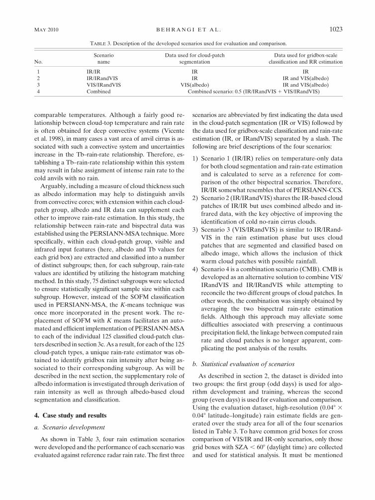
As shown in Table 3, four rain estimation scenarios

were developed and the performance of each scenario was

evaluated against reference radar rain rate. The first three

scenarios are abbreviated by first indicating the data used

in the cloud-patch segmentation (IR or VIS) followed by

the data used for gridbox-scale classification and rain-rate

estimation (IR, or IRandVIS) separated by a slash. The

following are brief descriptions of the four scenarios:

1) Scenario 1 (IR/IR) relies on temperature-only data

for both cloud segmentation and rain-rate estimation

and is calculated to serve as a reference for com-

parison of the other bispectral scenarios. Therefore,

IR/IR somewhat resembles that of PERSIANN-CCS.

2) Scenario 2 (IR/IRandVIS) shares the IR-based cloud

patches of IR/IR but uses combined albedo and in-

frared data, with the key objective of improving the

identification of cold no-rain cirrus clouds.

3) Scenario 3 (VIS/IRandVIS) is similar to IR/IRand-

VIS in the rain estimation phase but uses cloud

patches that are segmented and classified based on

albedo image, which allows the inclusion of thick

warm cloud patches with possible rainfall.

4) Scenario 4 is a combination scenario (CMB). CMB is

developed as an alternative solution to combine VIS/

IRandVIS and IR/IRandVIS while attempting to

reconcile the two different groups of cloud patches. In

other words, the combination was simply obtained by

averaging the two bispectral rain-rate estimation

fields. Although this approach may alleviate some

difficulties associated with preserving a continuous

precipitation field, the linkage between computed rain

rate and cloud patches is no longer apparent, com-

plicating the post analysis of the results.

b. Statistical evaluation of scenarios

As described in section 2, the dataset is divided into

two groups: the first group (odd days) is used for algo-

rithm development and training, whereas the second

group (even days) is used for evaluation and comparison.

Using the evaluation dataset, high-resolution (0.048 3

0.048 latitude–longitude) rain estimate fields are gen-

erated over the study area for all of the four scenarios

listed in Table 3. To have common grid boxes for cross

comparison of VIS/IR and IR-only scenarios, only those

grid boxes with SZA , 608 (daylight time) are collected

and used for statistical analysis. It must be mentioned

TABLE 3. Description of the developed scenarios used for evaluation and comparison.

No.

Scenario

name

Data used for cloud-patch

segmentation

Data used for gridbox-scale

classification and RR estimation

1 IR/IR IR IR

2 IR/IRandVIS IR IR and VIS(albedo)

3 VIS/IRandVIS VIS(albedo) IR and VIS(albedo)

4 Combined Combined scenario: 0.5 (IR/IRandVIS 1 VIS/IRandVIS)


that, in this study, the daytime hours are limited to only

6 h between 0900 and 1500 local solar time (LST) so that

3- and 6-hourly rain rates can be generated and com-

pared. Two groups of statistical indices are utilized to

evaluate the results. The categorical indices, from the con-

tingency table, are computed from the binary (0/1 or yes/

no) definition of rainfall events as determined by a 0.1

mm h21 threshold above which a rain event would be

considered to have occurred. The calculated indices are

equitable threat score (ETS), probability of detection

(POD), false-alarm ratio (FAR), and areal bias (BIASa).

The second group of statistical indices, quantitative indices,

is based on gridbox rain-rate values, which include corre-

lation coefficient (CORR), root-mean-square error (RMSe,

and quantitative bias (BIASq). Note that BIASa rep-

resents the ratio of satellite-derived rain area over the

observed rain area, whereas BIASq represents the ratio

using rain volume. Descriptions of the aforementioned

statistics are provided in appendix B. Table 4 provides

overall 3-h evaluation of the scenarios against radar at

a range of spatial resolutions: 0.048, 0.088, 0.128, and 0.248

(latitude–longitude). For each of the statistical indices,

except BIASa and BIASq, a performance gain metric

is reported, facilitating evaluation of albedo-included

scenarios (VIS/IRandVIS, IR/IRandVIS, and CMB)

against the reference IR-only scenario (IR/IR). For each

statistical index S, the performance gain metric of a

given scenario is defined as

Gain/Lossscenario (%) 5S

scenario� S

IR/IR

SIR/IR

3 100. (2)

Whether this index is considered as gain or loss depends

on whether an increase or decrease of the value of per-

formance measure is better or worse. For example, con-

sider FAR and POD; the former is said to have gained if

Eq. (2) yielded a negative number and the latter gains

when Eq. (2) produces a positive value.

The results shown in Table 4 demonstrate that in-

cluding albedo results in significant improvement in both

categorical and quantitative statistical indices in all dif-

ferent spatial scales. For the 0.048 bispectral scenarios

R/IRandVIS, VIS/IRandVIS, and CMB, CORR gains

are 20.1%, 17.6%, and 26% and ETS gains are 40.5%,

62.6%, and 65.9%, respectively. ETS scores allow for

equitable cross comparison (Schaefer 1990) and are less

sensitive to being ‘‘played’’ by systematic overestimation

or underestimation. Theoretically and as discussed in the

introduction, thick clouds contain both convective and

stratiform rain areas. Therefore, unlike IR-based cloud-

patch scenarios (IR/IR and IR/IRandVIS), VIS/IRandVIS

should contain almost all of the rain areas and account

for both temperature and albedo in discerning gridbox

rain-rate estimates. This explains why VIS/IRandVIS

outperforms both IR/IR and IR/IRandVIS scenarios in

delineating rain areas. Although IR/IR and IR/IRandVIS

share the same cloud patches, IR/IRandVIS shows con-

siderable improvements in POD, FAR, and ETS. How-

ever, IR/IRandVIS is associated with lower BIASa,

meaning that the rain area observed by IR/IRandVIS

is smaller than that of IR/IR. This can be attributed to

the two-stage estimation procedure. First, during the

IR-based cloud segmentation, warm rains are excluded.

TABLE 4. Overall 3-h statistics in a range of space resolution: note that reduction in value of FAR and RMSE is gain.

Categorical statistics (based on contingency table) Quantitative statistics

Scenario

Duration

(h)

Resolution

(km) ETS

ETS

gain

(%) POD

POD

gain

(%) FAR

FAR

gain

(%) BIASa CORR

CORR

gain

(%) RMSE

RMSE

gain

(%) BIASq

IR/IR 3 4 0.221 0.000 0.386 0.000 0.484 0.000 0.749 0.401 0.000 2.545 0.000 0.729

IR/IRandVIS 3 4 0.311 40.533 0.404 4.555 0.248 248.698 0.537 0.481 20.060 2.379 26.530 0.737

VIS/IRandVIS 3 4 0.360 62.585 0.512 32.428 0.316 234.622 0.748 0.471 17.579 2.413 25.178 0.822

CMB 3 4 0.367 65.883 0.537 38.898 0.334 231.025 0.806 0.505 25.958 2.290 210.027 0.780

IR/IR 3 8 0.229 0.000 0.412 0.000 0.468 0.000 0.774 0.408 0.000 2.340 0.000 0.728

IR/IRandVIS 3 8 0.304 32.591 0.406 21.408 0.226 251.711 0.524 0.549 34.486 2.103 210.130 0.737

VIS/IRandVIS 3 8 0.364 59.109 0.534 29.650 0.296 236.677 0.758 0.538 31.682 2.135 28.728 0.821

CMB 3 8 0.368 60.725 0.555 34.726 0.315 232.742 0.809 0.566 38.627 2.045 212.592 0.779

IR/IR 3 12 0.240 0.000 0.441 0.000 0.458 0.000 0.813 0.438 0.000 2.202 0.000 0.726

IR/IRandVIS 3 12 0.299 24.365 0.411 26.741 0.215 253.153 0.523 0.588 34.180 1.949 211.483 0.737

VIS/IRandVIS 3 12 0.365 52.062 0.550 24.739 0.285 237.857 0.769 0.575 31.226 1.983 29.916 0.819

CMB 3 12 0.366 52.603 0.569 29.074 0.304 233.581 0.818 0.603 37.524 1.900 213.704 0.778

IR/IR 3 24 0.267 0.000 0.500 0.000 0.420 0.000 0.861 0.508 0.000 1.910 0.000 0.723

IR/IRandVIS 3 24 0.288 7.635 0.427 214.535 0.199 252.678 0.533 0.661 29.945 1.663 212.913 0.736

VIS/IRandVIS 3 24 0.361 34.993 0.578 15.656 0.261 237.777 0.782 0.643 26.536 1.703 210.818 0.816

CMB 3 24 0.359 34.207 0.590 18.038 0.277 234.040 0.816 0.672 32.155 1.624 214.960 0.776


In the subsequent step (rain estimation from gridbox

classification), thin cold clouds are not mistakenly rec-

ognized as rain area. In other words, IR/IRandVIS pre-

vents assigning large false rains to remaining cold grid

boxes, which results in obtaining the lowest FAR among

all other scenarios. Note that IR/IRandVIS also shows

higher POD than IR/IR because of higher correct de-

tection of rain grid boxes in IR/IRandVIS. IR/IRandVIS

also outperforms IR/IR by demonstrating higher CORR

(20.1%–34.5% gain) and lower RMSE (from 26.5% to

212.9%; reduction in value is gain) and comparable

BIASq across all different spatial resolutions. As shown in

Table 4, although CMB does not show considerable im-

provement over VIS/IRandVIS for rain detection pur-

pose, it brings about almost the best quantitative statistics

among all other scenarios in different space scales.

Analysis of a number of individual storm events suggests

that CMB helps to moderate overestimated rain rates

obtained from either thick cirrus clouds or relatively

warm patches with extremely high albedo.

Table 5 presents the statistical measurements for 6-h

rain rates. The results are consistent with the 3-h sta-

tistics reported in Table 4, confirming that VIS/IRand-

VIS and CMB are effective scenarios across different

temporal and spatial resolutions. CMB consistently

shows the best gains for ETS, CORR, and RMSE with

the value of 49.5%, 27.6%, and 213.1%, respectively, at

6-h 0.248 resolution. IR/IRandVIS shows the best gain

for FAR with maximum gain of 252.2% (negative sign

represents FAR reduction) across different resolutions.

All scenarios, however, underestimate both areal extent

and volume of rainfall when compared to ground-based

radar observations. Part of this underestimation can be

attributed to early removal of warm (Tb . 253 K) or

dim (albedo , 0.4) grid boxes during cloud segmen-

tation stage, as explained in section 3a and shown in

Fig. 1.

Figure 5 provides a cross comparison of the statistical

indices of all four scenarios using 30-day evaluation of

6-h (0900–1500 LST), 0.048 resolution rain estimates

over the whole study area. The categorical and quanti-

tative statistical indices are shown in the left- and right-

side columns of Fig. 5, respectively. Although VIS/

IRandVIS and CMB show very similar rain detection

skills, both significantly and consistently exhibit higher

ETS, POD, and BIASa skills compared to IR/IRandVIS

and IR/IR scenarios. As shown in Fig. 4e, IR/IRandVIS

shows the best FAR and consistently performs better

than IR/IR in terms of ETS and POD. However, given

that a perfect BIASa score is 1, IR/IRandVIS displays

the worst BIASa value among all other scenarios. It is

important to recognize that a perfect BIASa score does

not necessarily guarantee a perfect match of rain/no-rain

pixels between observed and predicted fields. Figure 5b

implies that CMB has the best correlation with radar

rain rates, followed by VIS/IRandVIS. Unlike CMB,

VIS/IRandVIS does not show consistently superior RMSE

(Fig. 5d) among all other cases. However, comparison of

VIS/IRandVIS with CMB suggests that both scenarios

perform almost comparably. The poorest CORR and

RMSE are both attributed to IR/IR, followed by IR/

IRandVIS. This indicates that the IR/IR scenario can be

significantly improved by incorporating albedo informa-

tion to cloud-patch segmentation/classification phase,

TABLE 5. Overall 6-h statistics in a range of space resolution: note that reduction in value of FAR and RMSE is gain.

Categorical statistics (based on contingency table) Quantitative statistics

Scenario

Duration

(h)

Resolution

(km) ETS

ETS

gain

(%) POD

POD

gain

(%) FAR

FAR

gain

(%) BIASa CORR

CORR

gain

(%) RMSE

RMSE

gain

(%) BIASq

IR/IR 6 4 0.252 0.000 0.458 0.000 0.444 0.000 0.823 0.441 0.000 4.112 0.000 0.727

IR/IRandVIS 6 4 0.391 54.715 0.523 14.245 0.228 248.604 0.677 0.515 16.827 3.862 26.079 0.737

VIS/IRandVIS 6 4 0.438 73.494 0.649 41.774 0.298 232.973 0.924 0.502 13.770 3.922 24.637 0.822

CMB 6 4 0.442 75.198 0.676 47.717 0.315 228.964 0.988 0.535 21.290 3.747 28.876 0.779

IR/IR 6 8 0.258 0.000 0.481 0.000 0.425 0.000 0.837 0.444 0.000 3.795 0.000 0.726

IR/IRandVIS 6 h 8 0.385 49.320 0.530 10.148 0.209 250.929 0.669 0.577 29.863 3.455 28.962 0.737

VIS/IRandVIS 6 8 0.444 72.583 0.676 40.611 0.279 234.446 0.938 0.562 26.488 3.514 27.405 0.820

CMB 6 8 0.444 72.388 0.698 45.186 0.298 229.955 0.994 0.590 32.803 3.379 210.968 0.778

IR/IR 6 12 0.265 0.000 0.505 0.000 0.414 0.000 0.862 0.473 0.000 3.581 0.000 0.724

IR/IRandVIS 6 12 0.380 43.191 0.537 6.277 0.198 252.160 0.669 0.612 29.434 3.220 210.087 0.736

VIS/IRandVIS 6 12 0.444 67.446 0.691 36.772 0.268 235.409 0.943 0.596 26.018 3.282 28.361 0.819

CMB 6 12 0.440 66.088 0.711 40.693 0.288 230.461 0.998 0.624 31.878 3.154 211.913 0.778

IR/IR 6 24 0.286 0.000 0.557 0.000 0.382 0.000 0.901 0.539 0.000 3.135 0.000 0.720

IR/IRandVIS 6 h 24 0.364 27.266 0.554 20.557 0.186 251.389 0.680 0.679 25.992 2.779 211.353 0.735

VIS/IRandVIS 6 24 0.434 51.803 0.711 27.702 0.244 236.032 0.941 0.659 22.242 2.851 29.053 0.815

CMB 6 24 0.427 49.492 0.725 30.090 0.262 231.394 0.982 0.688 27.579 2.726 213.053 0.775


rain-rate estimation phase, or both. Figure 5f shows that

none of the scenarios consistently outperforms all others

with respect to bias. IR/IRandVIS shows overall lowest

BIASq, whereas VIS/IRandVIS presents overall larger

BIASq than other scenarios.

c. Event-scale analysis

To exemplify the analysis of the four described sce-

narios at event scale, a rain event at 1615 UTC 24 Au-

gust 2006 over Arizona is shown in Fig. 6. Instantaneous

maps of IR brightness temperature and albedo (Figs. 6a,b)

in conjunction with radar rain-rate map (Fig. 6c) show

the presence of a mesoscale convective system in the

center of the image, coupled with some warm rainfall at

the top-right corner of the studied area. Figure 6d

shows cloud patches segmented through implemen-

tation of the ITT approach on the IR brightness tem-

perature image. Albedo-based cloud patches are also

shown in Fig. 6g, which were obtained by applying

ITT approach to the smoothed albedo field (Fig. 6e).

Rain-rate maps of IR/IR, IR/IRandVIS, and VIS/

IRandVIS scenarios are shown in Figs. 6f,h,i below

their corresponding cloud-patch maps. Finally, the es-

timated rain-rate map from CMB is displayed in Fig. 6j.

Color-scale bars for the IR brightness temperature, al-

bedo, and rain-rate maps are collected in the center of

the right-side column.

As shown in Fig. 6d, the implementation of IR-based

cloud segmentation screens out all grid boxes with Tb .

253 K that may include rainfall (see zone A in Figs. 6a,c).

This results in relatively poor performance of IR/IRandVIS

and IR/IR scenarios in terms of their ability to capture

the observed rain areal extent. Visual comparison of IR/

IRandVIS (Fig. 6h), IR/IR (Fig. 6f), and radar rain-rate

(Fig. 6c) maps in addition to the suite of evaluation sta-

tistics (reported in Table 6) indicate that IR/IRandVIS

substantially performs better than IR/IR in terms of lo-

cating rain areas. Relative to IR/IR, more than 30%

gain in ETS, 29% gain in POD, and a noticeable im-

provement in BIASa are obtained by using bispectral in-

formation in the rain estimation phase (IR/IRandVIS),

although FAR does not show any significant gain. Albedo-

based segmentation (VIS/IRandVIS), on the other hand,

substantially scores better than IR/IRandVIS and IR/IR

FIG. 5. Evaluation statistics for all four scenarios using 30 days of 6-h (0900–1500 LST) high-

resolution (4 km) RR over the whole study area: (left) categorical statistics including (a) ETS,

(c) POD, (e) FAR, and (g) BIASa and (right) quantitative statistics including (b) CORR,

(d) RMSE, and (f) BIASq. Note that perfect score for both BIASa and BIASq is 1.


with more than 41% and 53% gains in ETS and POD,

respectively. VIS/IRandVIS also extends the detected

rain area to a size comparable to that of the ground radar

observation (BIASa 5 0.89). However, by detecting larger

rain areas, the albedo-based segmentation resulted in

higher FAR than Tb-based approached, with almost 25%

loss in skill compared to IR/IR. As expected, most of the

rain area is captured by VIS/IRandVIS; thus, the combi-

nation of VIS/IRandVIS and IR/IRandVIS does not show

significant change in rain detection scores. Although FAR

for CMB is increased to some extent (29% loss relative to

IR/IR), with about 49% gain in ETS, 64% gain in POD,

and BIASa 5 0.96, it can be argued that the combined

alternative serves as the best rain detector.

FIG. 6. Visual assessment of performances of the studied scenarios using a rain event at 1615 UTC 24 Aug 2006 over

Arizona: (a) IR Tb (K), (b) normalized albedo, (c) radar RR, (d) IR-based cloud patches, (e) smoothed albedo image

prior to cloud segmentation, (f) RR estimate from scenario IR/IR, (g) albedo-based cloud segmentation, (h) RR

estimate from scenario IR/IRandVIS, (i) RR estimate from scenario VIS/IRandVIS, and ( j) RR estimate from sce-

nario CMB. Note that columns are associated with (left) IR-based and (middle) albedo-based cloud patches.

TABLE 6. Statistics for the event-scale case study at 1615 UTC 24 Aug 2006 over Arizona, as shown in Fig. 6: note that reduction in value of

FAR and RMSE is gain.

Scenario ETS

ETS

gain (%) POD

POD

gain (%) FAR

FAR

gain (%) BIASa CORR

CORR

gain (%) RMSE

RMSE

gain (%) BIASq

IR/IR 0.282 0.000 0.413 0.000 0.230 0.000 0.536 0.463 0.000 2.520 0.000 0.650

IR/IRandVIS 0.368 30.496 0.533 29.056 0.224 22.609 0.687 0.510 10.151 2.460 22.381 0.910

VIS/IRandVIS 0.399 41.489 0.635 53.753 0.288 25.217 0.893 0.530 14.471 2.489 21.230 1.180

CMB 0.420 49.007 0.676 63.632 0.297 29.130 0.962 0.580 25.270 2.301 28.690 1.045


Figure 6 and Table 6 also demonstrate that CMB re-

sults in the best quantitative statistical indices with 25.3%

gain in CORR, 8.7% gain in RMSE, and a fairly rea-

sonable capture of the total volume of rainfall (BIASq 5

1.05). Although VIS/IRandVIS and IR/IRandVIS do

not show any significant improvement in RMSE, both

present substantial gains in CORR and capturing the

rainfall volume. The improved volumetric bias (BIASq)

for VIS/IRandVIS (1.18) and IR/IRandVIS (0.91), com-

pared to the traditional Tb-only approach (0.65), indicates

that overall albedo is also effective in supplementing

infrared-only data to capture a more realistic total

amount in addition to distribution and areal extent of

the rainfall.

5. Discussion

The method presented in this paper benefits from in-

frared and visible data not only for the purpose of cloud

segmentation and classification but also to generate more

accurate rainfall rates using a combination of the two.

The bispectral rain rate is obtained using PERSIANN-

MSA; therefore, it is extensible to multispectral data.

In other words, within each cloud patch, it is possible to

extract multispectral information for each grid box

and apply PERSIANN-MSA to extend the histogram

matching technique to multiple dimensions. As shown

in Behrangi et al. (2009a), multispectral information,

which is increasingly becoming available, can supple-

ment infrared-only data during both daytime and

nighttime.

Although incorporating the visible channel is prom-

ising, there are issues that need to be considered. First,

snow on the ground may pose a limitation during the

cloud-patch-type identification and rain-rate estimation

steps because it can be confused with thick clouds. Sec-

ond, the albedo normalization process used in this study

is simple, and it assumes that the reflected radiation field

is isotropic; thus, it is subject to errors. In addition, nor-

malization performance using the inverse cosine of SZA

deteriorates during the early morning and late afternoon

periods, as discussed in Behrangi et al. (2009b), which

limits the applicability of the method to grid boxes where

SZA , 608, as used in this study. A more rigorous ap-

proach of directly retrieving the cloud microphysical

properties from reflected solar radiation such as that pre-

sented in Nakajima and King (1990) and Nakajima et al.

(1991) can be investigated. Third, cloud reflectance is only

available during daylight hours, albeit for longer duration

during Northern Hemisphere summertime. As such, bis-

pectral algorithms are limited to a few hours in many re-

gions of the world. Finally, despite the fact that visible data

are almost globally available from constellation of GEO

satellites, no serious attempt has been made to collect and

process the data for users outside operational agencies

as is the case of IR (;11 mm) data that were made

available, at global scale, to the research community

through the efforts of the Climate Prediction Center

(CPC; Janowiak et al. 2001).

Despite some of the arguments in the literature against

incorporating visible channel into the operational pre-

cipitation algorithms, one should note that, depending on

location and time of year, significant amount of rainfall

events may occur during the daylight period. In many

regions of the world, rainfall volume and intensity peaks

during daytime and even in some cases during morning

and early afternoon (Hong et al. 2005; Sorooshian et al.

2002; Tian et al. 2007; Yang and Slingo 2001). However,

there remains a question as to whether the visible–infrared

rain estimates can serve different scientific communities.

On one hand, climatologists are more interested in the

quantitative and algorithmic consistency of the final pre-

cipitation product for both daytime and nighttime hours to

investigate long-term rainfall trends. Accordingly, multi-

spectral precipitation products that use VIS bands are

not necessarily adequate for the development of long-

term precipitation climatology. Operational hydrolo-

gists and flood forecasters, on the other hand, are very

interested in improving the accuracy of real-time rain-

rate estimates and the ability to accurately identify the

areal extent of precipitation at any time. As such, it is

likely that they will welcome any improvement, whether

it is at daytime, nighttime, or both.

6. Summary and conclusions

In this paper, two of our previously developed algo-

rithms, the cloud-patch-based PERSIANN-CCS and the

gridbox-based PERSIANN-MSA, were integrated. The

objective of this integrated method is to facilitate the in-

corporation of multispectral information into the cloud

segmentation–classification and rain estimation phases of

PERSIANN-CCS when coupled with the multispectral

technique of PERSIANN-MSA.

A bispectral experiment was performed in which one

reference infrared-only and three different bispectral

(visible–infrared) rain estimation scenarios were com-

pared. The goal of this comparison was to address existing

drawbacks of infrared-only techniques, which are re-

lated to their inability to (i) estimate warm rainfall and

(ii) screen out no-rain thin cirrus clouds. The first short-

coming may result in significant underestimation of the

total volume of rainfall, whereas the later may terminate

assigning rain to places with no rain. The proposed

approach combines the benefit of multispectral strate-

gies and the ability of cloud-patch-based algorithms to


consider the association of gridbox rain rates to their

corresponding cloud synoptic type.

Of the four scenarios, the baseline infrared-only sce-

nario (IR/IR) resembles that of the PERSIANN-CCS

technique, in which a fixed threshold 253 K is used to isolate

rain areas, segment clouds into number of distinct cloud

patches, classify the patches into a number of groups, and

subsequently estimate rain rate by establishing an IR

brightness temperature–rain-rate relationship for each

cloud-patch class using observed rain rate. This fixed

temperature threshold was shown to prevent IR-only

algorithms from capturing warm rainfalls. To couple

infrared data with albedo during daytime, three scenarios

were investigated. In the first scenario, a bispectral ap-

proach was developed that employs a temperature-based

cloud segmentation scheme with threshold 253 K (as in

PERSIANN-CCS) followed by a bispectral rain-rate es-

timation from each individual cloud-patch class (based

on PERSIANN-MSA). This approach was termed IR/

IRandVIS. The second bispectral scenario (VIS/IRandVIS)

also uses bispectral data for rain-rate estimation but

segments cloud patches using a smoothed image of cloud

albedo. Finally, the third bispectral scenario (CMB) is

obtained by combining IR/IRandVIS and VIS/IRandVIS

using arithmetic averaging.

Using 3 months (June–August 2006) of high-resolution

visible–infrared and radar rain-rate data over the eastern

and central conterminous United States, the scenarios

were trained utilizing odd-day data and subsequently

evaluated with data from even days. The comparison

included both categorical and quantitative statistical scores

over a range of temporal and spatial resolution. The results

indicate that overall CMB performs the best with respect

to identifying rain area as well as accurate estimation of

rain intensity. VIS/IRandVIS and IR/IRandVIS are sec-

ond and third, with IR/IR (temperature only) yielding the

least favorable performance measures. Improvement of

CMB over VIS/IRandVIS is found marginal, which sug-

gests that segmentation of clouds using their reflection

intensity is effective in expanding rain areas to include

warm rainfall prior to the rain-rate estimation phase. In

addition, albedo information supplements infrared-only

data to refine cloud-patch classes and establish more ro-

bust rain-rate estimates for each cloud-patch class.

Acknowledgments. Partial financial support is made

available from NASA Earth and Space Science Fellow-

ship (NESSF) Award (NNX08AU78H), NASA-NEWS

(Grant NNX06AF93G), NOAA/NESDIS GOES-R Pro-

gram Office (GPO), and NSF STC for Sustainability of

Semi-Arid Hydrology and Riparian Areas (SAHRA;

Grant EAR-9876800) programs. The authors thank

Mr. Dan Braithwaite for his technical assistance.

APPENDIX A

Cloud-Patch Feature Description

For a cloud patch P with gridbox brightness temper-

ature T(x, y), albedo A(x, y), and total gridbox count N,

the cloud-patch features listed in Table 1 are described

as follows:

1) Minimum temperature (Tmin):

Tmin 5 min[T(xi, y

i)], where i 2 P; at

i 5 c, T(xc, y

c) 5 Tmin.

2) Maximum albedo (Amax):

Amax 5 max[A(xi, y

i)], where i 2 P;

at i 5 r, A(xr, y

r) 5 Amax.

3) Mean temperature (Tmean):

Tmean 5�i2P

[T(xi, y

i)/N].

4) Mean albedo (Amean):

Amean 5 �i2P

[A(xi, y

i)/N].

5) Cloud-patch area (AREA):

AREA 5 gridbox resolution 3 N.

6) Slope parameter at Tmin (SMNT):

SMNT 5 �i2V5

c ,i6¼c[T(xi, yi)/(N

V5c� 1)] � T(xc, yc),

where Vc5 is a window size of 5 3 5 grid boxes cen-

tered on grid box r (corresponding with Amax) and

NV5

cis the number of grid boxes within Vc

5. Note that

SMNT is similar to the slope parameter calculated in

CST (Adler and Negri 1988) to remove no-rain cirrus.

7) Slope parameter at Amax (SMXA):

SMXA 5 �i2V5

c,i 6¼r[A(xi, yi)/(N

V5r� 1)] � A(xr, yr),

where Vr5 is a window size of 5 3 5 grid boxes cen-

tered on grid box r (corresponding with Amax). NV5

r

is number of grid boxes within Vr5.

8) Standard deviation of cloud-patch temperature

(STDT):

STDT

5 �i2P

[T(xi, y

i)� Tmean]0.5/(N � 1)

� �0.5

.

9) Mean value of local standard deviations of cloud-

patch temperature (MEAN5STDT

):

MEAN5STD

T5

�N

i51(STD5

T)i

N,


where STDT5 is the standard deviation of cloud-top

temperature within window size of 5 3 5 grid boxes

centered on grid box i.

10) Standard deviation of local standard deviations of

cloud-patch temperature (STDT5 ):

STD5STD

T5 �

N

i51

[(STD5T)

i�MEAN5

STDT]

N � 1

8<:

9=;

0.5

.

APPENDIX B

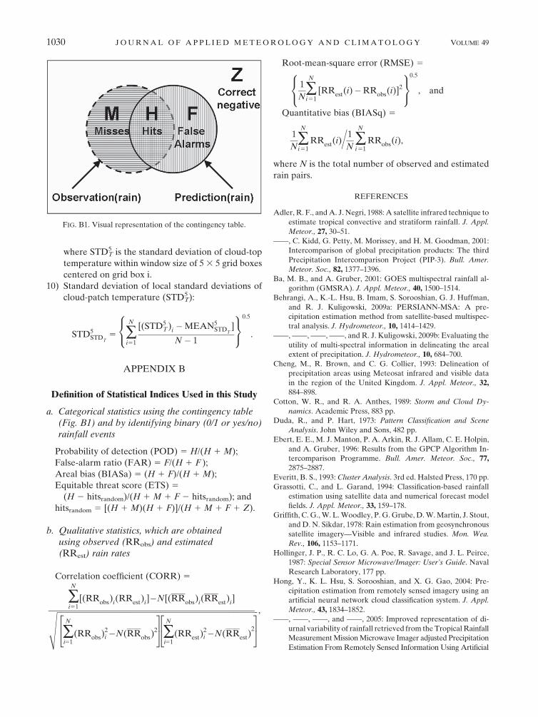
Definition of Statistical Indices Used in this Study

a. Categorical statistics using the contingency table(Fig. B1) and by identifying binary (0/1 or yes/no)rainfall events

Probability of detection (POD) 5 H/(H 1 M);

False-alarm ratio (FAR) 5 F/(H 1 F );

Areal bias (BIASa) 5 (H 1 F)/(H 1 M);

Equitable threat score (ETS) 5

(H 2 hitsrandom)/(H 1 M 1 F 2 hitsrandom); and

hitsrandom 5 [(H 1 M)(H 1 F)]/(H 1 M 1 F 1 Z).

b. Qualitative statistics, which are obtainedusing observed (RRobs) and estimated(RRest) rain rates

Correlation coefficient (CORR) 5

�N

i51[(RR

obs)

i(RR

est)

i]�N[(RR

obs)

i(RR

est)

i]

ffiffiffiffiffiffiffiffiffiffiffiffiffiffiffiffiffiffiffiffiffiffiffiffiffiffiffiffiffiffiffiffiffiffiffiffiffiffiffiffiffiffiffiffiffiffiffiffiffiffiffiffiffiffiffiffiffiffiffiffiffiffiffiffiffiffiffiffiffiffiffiffiffiffiffiffiffiffiffiffiffiffiffiffiffiffiffiffiffiffiffiffiffiffiffiffiffiffiffiffiffiffiffiffiffiffi�N

i51(RR

obs)2

i �N(RRobs

)2

24

35�

N

i51(RR

est)2

i �N(RRest

)2

24

35

vuuut,

Root-mean-square error (RMSE) 5

1

N�N

i51[RRest(i)�RRobs(i)]2

8<:

9=;

0.5

, and

Quantitative bias (BIASq) 5

1

N�N

i51RRest(i)= 1

N�N

i51RRobs(i),

where N is the total number of observed and estimated

rain pairs.

REFERENCES

Adler, R. F., and A. J. Negri, 1988: A satellite infrared technique to

estimate tropical convective and stratiform rainfall. J. Appl.

Meteor., 27, 30–51.

——, C. Kidd, G. Petty, M. Morissey, and H. M. Goodman, 2001:

Intercomparison of global precipitation products: The third

Precipitation Intercomparison Project (PIP-3). Bull. Amer.

Meteor. Soc., 82, 1377–1396.

Ba, M. B., and A. Gruber, 2001: GOES multispectral rainfall al-

gorithm (GMSRA). J. Appl. Meteor., 40, 1500–1514.

Behrangi, A., K.-L. Hsu, B. Imam, S. Sorooshian, G. J. Huffman,

and R. J. Kuligowski, 2009a: PERSIANN-MSA: A pre-

cipitation estimation method from satellite-based multispec-

tral analysis. J. Hydrometeor., 10, 1414–1429.

——, ——, ——, ——, and R. J. Kuligowski, 2009b: Evaluating the

utility of multi-spectral information in delineating the areal

extent of precipitation. J. Hydrometeor., 10, 684–700.

Cheng, M., R. Brown, and C. G. Collier, 1993: Delineation of

precipitation areas using Meteosat infrared and visible data

in the region of the United Kingdom. J. Appl. Meteor., 32,884–898.

Cotton, W. R., and R. A. Anthes, 1989: Storm and Cloud Dy-

namics. Academic Press, 883 pp.

Duda, R., and P. Hart, 1973: Pattern Classification and Scene

Analysis. John Wiley and Sons, 482 pp.

Ebert, E. E., M. J. Manton, P. A. Arkin, R. J. Allam, C. E. Holpin,

and A. Gruber, 1996: Results from the GPCP Algorithm In-

tercomparison Programme. Bull. Amer. Meteor. Soc., 77,

2875–2887.

Everitt, B. S., 1993: Cluster Analysis. 3rd ed. Halsted Press, 170 pp.

Grassotti, C., and L. Garand, 1994: Classification-based rainfall

estimation using satellite data and numerical forecast model

fields. J. Appl. Meteor., 33, 159–178.

Griffith, C. G., W. L. Woodley, P. G. Grube, D. W. Martin, J. Stout,

and D. N. Sikdar, 1978: Rain estimation from geosynchronous

satellite imagery—Visible and infrared studies. Mon. Wea.

Rev., 106, 1153–1171.

Hollinger, J. P., R. C. Lo, G. A. Poe, R. Savage, and J. L. Peirce,

1987: Special Sensor Microwave/Imager: User’s Guide. Naval

Research Laboratory, 177 pp.

Hong, Y., K. L. Hsu, S. Sorooshian, and X. G. Gao, 2004: Pre-

cipitation estimation from remotely sensed imagery using an

artificial neural network cloud classification system. J. Appl.

Meteor., 43, 1834–1852.

——, ——, ——, and ——, 2005: Improved representation of di-

urnal variability of rainfall retrieved from the Tropical Rainfall

Measurement Mission Microwave Imager adjusted Precipitation

Estimation From Remotely Sensed Information Using Artificial

FIG. B1. Visual representation of the contingency table.


Neural Networks (PERSIANN) system. J. Geophys. Res., 110,

D06102, doi:10.1029/2004JD005301.

Hou, A., G. S. Jackson, C. Kummerow, and J. M. Shepherd, 2008:

Global precipitation measurement. Precipitation: Advances in

Measurement, Estimation, and Prediction, S. Michaelides, Ed.,

Springer, 131–170.

Hsu, K. L., X. G. Gao, S. Sorooshian, and H. V. Gupta, 1997:

Precipitation estimation from remotely sensed information

using artificial neural networks. J. Appl. Meteor., 36, 1176–

1190.

——, H. V. Gupta, X. G. Gao, and S. Sorooshian, 1999: Estimation

of physical variables from multichannel remotely sensed im-

agery using a neural network: Application to rainfall estima-

tion. Water Resour. Res., 35, 1605–1618.

Huffman, G. J., and Coauthors, 2007: The TRMM Multisatellite

Precipitation Analysis (TMPA): Quasi-global, multiyear,

combined-sensor precipitation estimates at fine scales. J. Hy-

drometeor., 8, 38–55.

Janowiak, J. E., R. J. Joyce, and Y. Yarosh, 2001: A real-time

global half-hourly pixel-resolution infrared dataset and its

applications. Bull. Amer. Meteor. Soc., 82, 205–217.

Joyce, R. J., J. E. Janowiak, P. A. Arkin, and P. Xie, 2004:

CMORPH: A method that produces global precipitation es-

timates from passive microwave and infrared data at high

spatial and temporal resolution. J. Hydrometeor., 5, 487–503.

Kidd, C., D. R. Kniveton, M. C. Todd, and T. J. Bellerby, 2003:

Satellite rainfall estimation using combined passive micro-

wave and infrared algorithms. J. Hydrometeor., 4, 1088–

1104.

King, P. W. S., W. D. Hogg, and P. A. Arkin, 1995: The role of

visible data in improving satellite rain-rate estimates. J. Appl.

Meteor., 34, 1608–1621.

Kohonen, T., 1984: Self Organization and Associative Memory.

Springer-Verlag, 255 pp.

Kuligowski, R. J., 2002: A self-calibrating real-time GOES rainfall

algorithm for short-term rainfall estimates. J. Hydrometeor., 3,

112–130.

Kurino, T., 1997: A satellite infrared technique for estimating

‘‘deep/shallow’’ precipitation. Adv. Space Res., 19, 511–514.

Lin, Y., and K. E. Mitchell, 2005: The NCEP stage II/IV hourly

precipitation analyses: Development and applications. Pre-

prints, 19th Conf. on Hydrology, San Diego, CA, Amer. Me-

teor. Soc., 1.2. [Available online at http://ams.confex.com/ams/

pdfpapers/83847.pdf.]

Lovejoy, S., and G. L. Austin, 1979: The delineation of rain areas

from visible and IR satellite data for GATE and mid-latitudes.

Atmos.—Ocean, 17, 77–92.

MacQueen, J. B., 1967: Some methods for classification and anal-

ysis of multivariate observations. Proc. Fifth Berkeley Symp.

on Mathematical Statistics and Probability, Vol. 1, Berkeley,

CA, University of California Press, 281–297.

Maddox, R. A., J. Zhang, J. J. Gourley, and K. W. Howard, 2002:

Weather radar coverage over the contiguous United States.

Wea. Forecasting, 17, 927–934.

Manobianco, J., S. Koch, V. M. Karyampudi, and A. J. Negri, 1994:

The impact of assimilating satellite-derived precipitation rates

on numerical simulations of the ERICA IOP 4 cyclone. Mon.

Wea. Rev., 122, 341–365.

Martin, D. W., B. Goodman, T. J. Schmit, and E. C. Cutrim, 1990:

Estimation of daily rainfall over the Amazon basin. J. Geo-

phys. Res., 95, 17 043–17 050.

Nakajima, T., and M. D. King, 1990: Determination of the optical

thickness and effective particle radius of clouds from reflected

solar radiation measurements. Part I: Theory. J. Atmos. Sci.,

47, 1878–1893.

——, ——, J. D. Spinhirne, and L. F. Radke, 1991: Determination

of the optical thickness and effective particle radius of clouds

from reflected solar radiation measurements. Part II: Marine

stratocumulus observations. J. Atmos. Sci., 48, 728–751.

Negri, A. J., R. F. Adler, and P. J. Wetzel, 1984: Rain estimation

from satellites—An examination of the Griffith–Woodley

technique. J. Climate Appl. Meteor., 23, 102–116.

O’Sullivan, F., C. H. Wash, M. Stewart, and C. E. Motell, 1990:

Rain estimation from infrared and visible GOES satellite data.

J. Appl. Meteor., 29, 209–223.

Qiu, D., and A. C. Tamhane, 2007: A comparative study of the K-

means algorithm and the normal mixture model for clustering:

Univariate case. J. Stat. Plann. Inference, 137, 3722–3740.

Rosenfeld, D., and I. M. Lensky, 1998: Satellite-based insights into

precipitation formation processes in continental and maritime

convective clouds. Bull. Amer. Meteor. Soc., 79, 2457–2476.

Schaefer, J. T., 1990: The critical success index as an indicator of

warning skill. Wea. Forecasting, 5, 570–575.

Sorooshian, S., K. L. Hsu, X. Gao, H. V. Gupta, B. Imam, and

D. Braithwaite, 2000: Evaluation of PERSIANN system satellite-

based estimates of tropical rainfall. Bull. Amer. Meteor. Soc., 81,2035–2046.

——, X. Gao, K. Hsu, R. A. Maddox, Y. Hong, H. V. Gupta, and

B. Imam, 2002: Diurnal variability of tropical rainfall retrieved

from combined GOES and TRMM satellite information.

J. Climate, 15, 983–1001.

Tian, Y., C. D. Peters-Lidard, B. J. Choudhury, and M. Garcia,

2007: Multitemporal analysis of TRMM-based satellite pre-

cipitation products for land data assimilation applications.

J. Hydrometeor., 8, 1165–1183.

Todd, M. C., C. Kidd, D. Kniveton, and T. J. Bellerby, 2001: A

combined satellite infrared and passive microwave technique

for estimation of small-scale rainfall. J. Atmos. Oceanic

Technol., 18, 742–755.

Tsonis, A. A., and G. A. Isaac, 1985: On a new approach for in-

stantaneous rain area delineation in the mid-latitudes using

GOES data. J. Climate Appl. Meteor., 24, 1208–1218.

Turk, F. J., and S. D. Miller, 2005: Toward improved character-

ization of remotely sensed precipitation regimes with MODIS/

AMSR-E blended data techniques. IEEE Trans. Geosci.

Remote Sens., 43, 1059–1069.

——, E. E. Ebert, H. J. Oh, B. J. Sohn, V. Levizzani, E. A. Smith,

and R. R. Ferraro, 2003: Validation of an operational global

precipitation analysis at short time scales. Preprints, 12th

Conf. Satellite Meteorology and Oceanography, Long Beach,

CA, Amer. Meteor. Soc., JP1.2. [Available online at http://

ams.confex.com/ams/pdfpapers/56865.pdf.]

Vicente, G. A., R. A. Scofield, and W. P. Menzel, 1998: The op-

erational GOES infrared rainfall estimation technique. Bull.

Amer. Meteor. Soc., 79, 1883–1898.

Woodley, W. L., C. G. Griffith, J. S. Griffin, and S. C. Stromatt,

1980: The inference of GATE convective rainfall from SMS-1

imagery. J. Appl. Meteor., 19, 388–408.

Wu, R., J. A. Weinman, and R. T. Chin, 1985: Determination of

rainfall rates from GOES satellite images by a pattern rec-

ognition technique. J. Atmos. Oceanic Technol., 2, 314–330.

Xu, L., S. Sorooshian, X. Gao, and H. V. Gupta, 1999: A cloud-

patch technique for identification and removal of no-rain clouds

from satellite infrared imagery. J. Appl. Meteor., 38, 1170–1181.

Yang, G.-Y., and J. Slingo, 2001: The diurnal cycle in the tropics.

Mon. Wea. Rev., 129, 784–801.


Daytime Precipitation Estimation Using Bispectral Cloud ...

Documents