David Giles Bayesian Econometricsweb.uvic.ca/~dgiles/blog/Bayes_Slides_New_8.pdf3 • Metropolis et al. (1953) proposed the basic method, and proved its properties when the "proposal

1

David Giles

Bayesian Econometrics

8. The Metropolis-Hastings Algorithm

(Nicholas Metropolis, 1915 – 1999)

W. Keith Hastings, 1930 -

Ph.D., U of T (1962)

UVic Math. & Stats., 1971 - 1992

2

• A generalization of the Gibbs Sampler.

• Very useful when the conditional posteriors are messy and non-standard.

• Incorporates the ideas behind "Acceptance-Rejection" sampling.

• Basic idea:

(i) Target density is 𝜋(𝑥).

(ii) Choose a "Proposal distribution", q( . ).

(iii) Construct a Markov chain for X that is ergodic and stationary

with respect to 𝜋. That is, if X(t) ~ 𝜋(𝑥), then X(t+1) ~ 𝜋(𝑥), and

therefore X(t) converges in distribution to 𝜋( . ).

(iv) Rather than aiming at the "big picture" immediately, as an accept-reject

algorithm does, we construct a progressive picture of the target

distribution, proceeding by local exploration of the X space until

(hopefully) all the regions of interest have been uncovered.

3

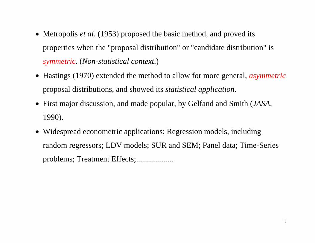
• Metropolis et al. (1953) proposed the basic method, and proved its

properties when the "proposal distribution" or "candidate distribution" is

symmetric. (Non-statistical context.)

• Hastings (1970) extended the method to allow for more general, asymmetric

proposal distributions, and showed its statistical application.

• First major discussion, and made popular, by Gelfand and Smith (JASA,

1990).

• Widespread econometric applications: Regression models, including

random regressors; LDV models; SUR and SEM; Panel data; Time-Series

problems; Treatment Effects;...................

4

Overview of the Metropolis-Hastings algorithm

• We want to draw from a density, 𝜋( . ), whose kernel is �̅�( . ).

• Given 𝑋(𝑡) = 𝑥(𝑡):

(1) Generate 𝑌𝑡~ 𝑞(𝑦 |𝑥(𝑡))

(2) Assign: 𝑋(𝑡+1) = { 𝑌𝑡 ; 𝑤𝑖𝑡ℎ 𝑝𝑟𝑜𝑏𝑎𝑏𝑖𝑙𝑖𝑡𝑦 𝜌(𝑥(𝑡), 𝑌𝑡)

𝑥(𝑡) ; 𝑤𝑖𝑡ℎ 𝑝𝑟𝑜𝑏𝑎𝑏𝑖𝑙𝑖𝑡𝑦 1 − 𝜌(𝑥(𝑡), 𝑌𝑡)

where 𝜌(𝑥, 𝑦) = 𝑚𝑖𝑛. {1 ,�̅�(𝑦)

�̅�(𝑥)

𝑞(𝑥 |𝑦)

𝑞(𝑦 |𝑥)}.

(3) Iterate, and discard a "burn-in" part of the chain.

5

Note:

(i) At step (2) we only need the kernel of the target distribution, as the

normalizing constant would cancel out in any case.

(ii) We have to choose the "proposal density", q( . ), and the start value.

(iii) These choices can affect the way in which the sampler explores the space,

& hence it can affect final results.

(iv) The Gibbs Sampler turns out to be a special case of M-H, where we always

take the step in the chain, and never repeat an x value.

6

Example

• Generate random values from a "perturbed Normal" distribution, using the

Metropolis algorithm.

• 𝑝(𝑥) ∝ 𝑠𝑖𝑛2(𝑥) × 𝑠𝑖𝑛2(2𝑥) × 𝜙(𝑥)

• Use U[x-α , x+α] as the "proposal density": 𝑞(𝑦 |𝑥) = (1

2𝛼) .

• R code: One function for the target distribution, and one for the transition

step.

target<- function(x) {

sin(x)^2*sin(2*x)^2*dnorm(x)

}

7

metropolis<- function(x,alpha) {

y<- runif(1,x-alpha,x+alpha)

if (runif(1) > min(1 , target(y)/target(x))) y=x

return(y)

}

set.seed(1234)

T<- 10^4

x<- rep(3.14,T)

alpha<- 1

for (t in 2:T) x[t]=metropolis(x[t-1], alpha)

plot(density(x), main="Metropolis-Hastings: Perturbed Normal", xlab="x", ylab="f

(x )", col="red", lwd="3")

8

9

However, if we set 𝛼 = 0.1:

Some choices of the proposal kernel work better than others!

10

Example

• Generate Beta random variables using Metropolis algorithm.

• Use N[0 , 1] as the "proposal density".

• R code:

set.seed(1234)

nrep<- 51000

burnin<- 1000

x<- vector(length=nrep)

x<-runif(nrep,0,1)

alpha<- 2

gamma<- 3

accept<- 0

11

# Start of the Metropolis algorithm

for (i in 2:nrep) {

u1<- runif(1,0,1)

u2<- runif(1,0,1)

if ( u1<= min(1,(u2^(alpha-1)*(1-u2)^(gamma-1))/x[(i-1)]^(alpha-1) /(1-x[(i-

1)])^(gamma-1))) {

x[i]<- u2

accept<- accept+1

}

else {

x[i]<-x[(i-1)]

}

}

# End of the Metropolis algorithm

12

# Present & summarize the results:

h<- hist(x[(burnin+1):nrep], prob=TRUE, main="Metropolis Simulation of Beta

Random Variables",sub="(True Beta p.d.f. Added)", xlab="x", ylab="p( x )",

col="pink")

xfit<- seq(0,1,length=101)

yfit<- dbeta(xfit,alpha,gamma)

lines(xfit, yfit, col="blue", lwd=2)

summary(x[(burnin+1):nrep]) ; var(x[(burnin+1):nrep])

# True mean & variance

c(alpha/(alpha+gamma) , alpha*gamma/(alpha+gamma+1)/(alpha+gamma)^2)

# Acceptance Rate (%)

accept / nrep*100

13

14

15

Example

• Metropolis algorithm to generate for N[0,1].

• A function for the Metropolis sampler for this problem is given below.

• The chain is initialised at zero, and at each stage a U[-α , α] innovation is

proposed.

• That is, the "candidate" distribution is U[-α , α].

• We'll illustrate with α = 1.

• We'll get a well-mixing chain, and a reasonably normal distribution for the

values.

• Other choices of α will not affect the stationarity of the distribution, but will

affect the rate of mixing of the chain.

16

norm<- function (n, alpha) {

vec <- vector("numeric", n)

x <- 0

vec[1] <- x

for (i in 2:n) {

innov <- runif(1, -alpha, alpha)

can <- x + innov

aprob <- min(1, dnorm(can)/dnorm(x))

u <- runif(1)

if (u < aprob)

x <- can

vec[i] <- x

}

vec }

17

# So, innov is a uniform random innovation and can is the candidate point. aprob

is the acceptance probability.

# The decision on whether or not to accept is then carried out on the basis of

whether or not a U(0,1) is less than the acceptance probability.

nrep<- 55000

burnin<- 5000

normvec<- norm(nrep,1) # Call the Metropolis function

par(mfrow=c(2,1))

plot(ts(normvec[(burnin+1):nrep]), ylab="Draw")

hist(normvec[(burnin+1):nrep],30, main="Simulated N[0,1]", xlab="x", ylab="p( x

)")

par(mfrow=c(1,1))

summary(normvec[(burnin+1):nrep]) ; var(normvec[(burnin+1):nrep])

18

19

N[0 , 1] ??

20

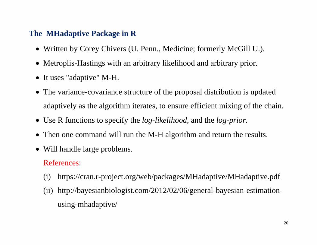
The MHadaptive Package in R

• Written by Corey Chivers (U. Penn., Medicine; formerly McGill U.).

• Metroplis-Hastings with an arbitrary likelihood and arbitrary prior.

• It uses "adaptive" M-H.

• The variance-covariance structure of the proposal distribution is updated

adaptively as the algorithm iterates, to ensure efficient mixing of the chain.

• Use R functions to specify the log-likelihood, and the log-prior.

• Then one command will run the M-H algorithm and return the results.

• Will handle large problems.

References:

(i) https://cran.r-project.org/web/packages/MHadaptive/MHadaptive.pdf

(ii) http://bayesianbiologist.com/2012/02/06/general-bayesian-estimation-

using-mhadaptive/

21

Simple Regression Example

• Based on an example given by Corey Chivers .

• 𝑦𝑖 = 𝛼 + 𝛽𝑥𝑖 + 𝜀𝑖 ; 𝜀𝑖 ~ 𝑁[0 , 𝜎2] ; i = 1, 2, ...., n

• 𝑝(𝛼, 𝛽, 𝜎) = 𝑝(𝛼)𝑝(𝛽)𝑝(𝜎)

• 𝑝(𝛼) = 𝑁[0 , 𝜎𝛼] ; 𝜎𝛼 is assigned

• 𝑝(𝛽) = 𝑁[0 , 𝜎𝛽] ; 𝜎𝛽 is assigned

• 𝑝(𝜎) = 𝐺𝑎𝑚𝑚𝑎[𝑎 , 𝑏] ; a and b are assigned

• In the illustration below, these priors are very "flat".

• So, the results are similar to MLE.

• By changing the parameters of the priors we can see the effects on the

marginal posterior results.

• Here is the R code:

22

library(MHadaptive)

set.seed(1234) # Function for log-likelihood

li_reg<-function(pars,data) {

a<-pars[1] #intercept

b<-pars[2] #slope

sd_e<-pars[3] #error s.d.

if(sd_e<=0) {return(NaN)}

pred <- a + b * data[,1]

log_likelihood<-sum( dnorm(data[,2],pred,sd_e, log=TRUE) )

log_prior<- prior_reg(pars) # Call up the function for log-prior

return(log_likelihood + log_prior) } # Return joint log-posterior

23

prior_reg<-function(pars) # Function for log-prior

{

a<-pars[1] #intercept

b<-pars[2] #slope

sigma<-pars[3] #error s.d.

prior_a<-dnorm(a,0,100,log=TRUE) # fairly non-informative (flat) priors on all

prior_b<-dnorm(b,0,100,log=TRUE) # parameters.

prior_sigma<-dgamma(sigma,1,1/100,log=TRUE)

return(prior_a + prior_b + prior_sigma) # Returns the joint log-prior

}

24

x<- runif(30,5,15)

y<- x+rnorm(30,0,5) ##Slope=1, intercept=0, sigma=5

d<- cbind(x,y)

par(mfrow=c(1,1))

plot(x,y, main="Scatter Plot for Data", xlab="x", ylab="y")

nrep<- 55000

burnin<- 5000

mcmc_r<-Metro_Hastings(li_func=li_reg,pars=c(1,1,2),

par_names=c('a','b','sigma'),data=d, iterations=nrep, burn_in=burnin)

25

post<- mcmc_r[[1]]

post_a<- post[,1]

post_b<- post[,2]

post_sigma<- post[,3]

# Is the Burn-in period long enough?

# Rolling mean diagnostics:

rmean_a<- vector(length=burnin)

rmean_b<- vector(length=burnin)

rmean_sigma<- vector(length=burnin)

26

for (i in 1:burnin) {

rmean_a[i]<- mean(post_a[1:i])

rmean_b[i]<- mean(post_b[1:i])

rmean_sigma[i]<- mean(post_sigma[1:i])

}

par(mfrow=c(1,1))

plot(rmean_a, col="green", main="Rolling Means for a", xlab="Burn-in

Replications", ylab="Mean of a")

plot(rmean_b, col="red", main="Rolling Means for b", xlab="Burn-in

Replications", ylab="Mean of b")

plot(rmean_sigma, col="blue", main="Rolling Means for sigma", xlab="Burn-in

Replications", ylab="Mean of sigma")

27

par(mfrow=c(3,3))

plotMH(mcmc_r)

BCI(mcmc_r)

summary(post_a[(burnin+1):nrep])

summary(post_b[(burnin+1):nrep])

summary(post_sigma[(burnin+1):nrep])

# Compare with the MLE results

mle<- lm(y~ x)

summary(mle)

28

29

30

31

32

33

34

35

Marginal Posterior Means: -9.46 4 ; 1.761 ; 4.386

36

Change the prior

prior_a<- dnorm(a,0,1,log=TRUE) ; prior_b<-dnorm(b,0,1,log=TRUE)

prior_sigma<- dgamma(sigma,1,1,log=TRUE)

Marginal Posterior Means: -0.879 ; 0.929 ; 4.650