DAVID BURCH THIRD EDITION - Starpath School of Navigation

Starpath Publications, Seattle WAwww.starpathpublications.com

MO

DERN

MA

RINE W

EATH

ERTH

IRD ED

ITION

BU

RCH

“A thoughtfully and masterfully crafted work. It will be my prime recommendation of a book focusing specifi cally on the application of weather information and knowledge for maritime interests, whatever the size and purpose of the vessel. David thoroughly explores the essentials of meteorology, and does so in a fascinating manner. Reading and absorbing these principles and applications will lead to safer, faster and more efficient passages.”—Jeff Renner, Meteorologist, King 5 TV, Seattle,WA.

“I have chosen this book as the defi nitive text for the wardroom of my U.S. Navy Destroyer. Superior explanations that are as useful for the professional naval offi cer as they are for the coastal pleasure cruiser or blue water sailor. Consistent with all of David Burch’s texts: Easy to read, fascinating, and the absolute best resource.” —CDR Tate Westbrook, CO USS Spruance (DDG111)

“First class reference book on the subject of marine weather and the information it contains will help every sailor, every day!” — Peter Isler, two-time America’s Cup winning navigator

“An essential reference for the coastal and offshore sailor. It goes far beyond the traditional marine weather books. …an excellent job of laying proper foundations for understanding marine weather, and bringing clarity to a complex topic.” —Jim Corenman, developer of Saildocs and SailMail

“The defi nitive text for those wanting to learn more about marine meteorology. …David Burch should be applauded for this beautiful piece of work.” —Kenn Batt, Australian Bureau of Meteorology, Sydney to Hobart Race weather briefer

“An instant classic. If you own one book about weather this is it. If you want to make your own intelligent forecast and pick-up local knowledge like a local, you will fi nd all the information in this most excellent book.” —Philippe Kahn, CEO, FullPower Technologies, Doublehanded Transpacific record holder

“A new and truly extraordinary treatise on an age old subject. Principles and scientific conclusions expertly revealed in layman’s terms.” —Roger Jones, Director, The Navigation Foundation

“…points out where to fi nd the best stuff quickly, how to read weather maps, digest storms warnings, read clouds, interpret GRIB data and satellite winds to win yacht races or sail comfortably across an ocean.” –Bob McDavitt, New Zealand MetService

PRAISE FOR MODERN MARINE WEATHER...

Scan for related resources.

BU

RCH

THIRD

EDITIO

NTH

IRD ED

ITION

THIRD

EDITIO

NTH

IRD ED

ITION

THIRD

EDITIO

N

“An invaluable resource that belongs in the wheelhouse alongside Bowditch.”

— Lee Chesneau, NWS Forecaster

MODERN MARINE WEATHERFrom Time-honored Traditional Knowledge to the Latest Technology

DAVID BURCH

THIRD EDITION

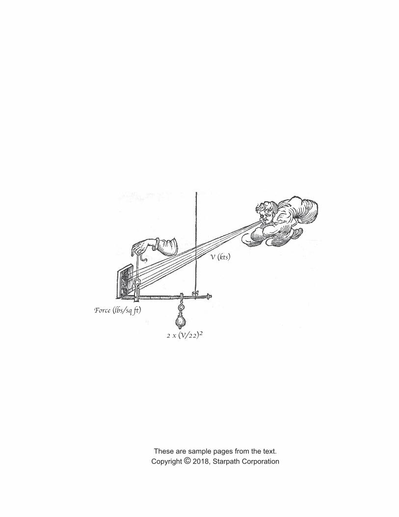
V (kts)

2 x (V/22)2

Force (lbs/sq ft)

These are sample pages from the text.Copyright © 2018, Starpath Corporation

v

ContentsPreface to the first edition ................................................................................................... viiPreface to the second edition .............................................................................................. viiPreface to the third edition ................................................................................................. viiAcknowledgements ............................................................................................................ viiiForeword ............................................................................................................................. ix

INTRODUCTION .................................................................................11.1 Overview ............................................................................................................................11.2 Role of Marine Weather .................................................................................................. 21.3 Elements of Marine Weather .......................................................................................... 41.4 Terminology and Glossaries ........................................................................................... 61.5 Wind Terms and Symbols ............................................................................................... 61.6 Quick Look at Resources ................................................................................................. 91.7 Units and Time Conversions ..........................................................................................12

PRESSURE AND WIND ..................................................................... 152.1 What Makes the Wind ....................................................................................................152.2 Pressure and Barometers ...............................................................................................212.3 Properties of Highs and Lows ....................................................................................... 252.4 Figuring Winds From Isobars .......................................................................................262.5 Apparent Wind to True Wind .......................................................................................312.6 Getting Started on GRIB Files ......................................................................................34

GLOBAL WINDS AND CURRENTS ....................................................413.1 Warm Air Rises ...............................................................................................................413.2 Hadley Cells and Global Winds ....................................................................................423.3 Winds Aloft ....................................................................................................................493.4 Atmosphere, Air Masses and Stability .......................................................................... 553.5 Water —The Fuel of the Atmosphere ............................................................................ 613.6 Primary Ocean Currents ...............................................................................................663.7 Ocean Current Models ...................................................................................................71

STRONG WIND SYSTEMS.................................................................774.1 Introduction to Strong Wind ......................................................................................... 774.2 Satellite Winds ..............................................................................................................804.3 Fronts and Low Formation ........................................................................................... 874.4 Types of Lows ................................................................................................................964.5 Tropical Storms and Hurricanes .................................................................................1014.6 Squalls ......................................................................................................................... 1084.7 Sides of a Tropical Storm ............................................................................................. 1154.8 Storm Avoidance Maneuvering ...................................................................................118

CLOUDS, FOG, AND SEA STATE ..................................................... 1215.1 Cloud Notes for Mariners .............................................................................................1215.2 Sample Cloud Pictures ................................................................................................ 1265.3 Fog ............................................................................................................................... 1265.4 Wave Notes for Mariners ............................................................................................ 130

WIND AND TERRAIN ..................................................................... 1376.1 The Varied Effects of Land on Wind ............................................................................1376.2 Isobars Crossing Channels .......................................................................................... 1426.3 Wind Forecasts Near Land ..........................................................................................147

vi

WORKING WITH WEATHER MAPS ...............................................1497.1 Overview of Weather Maps ......................................................................................... 1497.2 Using Weather Maps ................................................................................................... 1507.3 Practice Reading Weather Maps ..................................................................................1577.4 Georeferencing Image Files ........................................................................................ 1607.5 Global and Regional Models ..................................................................................... 1667.6 Use of 500-mb Maps .................................................................................................... 1717.7 Ship Reports .................................................................................................................176

SOURCES OF WEATHER DATA ...................................................... 1798.1 Overview .......................................................................................................................1798.2 Climatic Sources for Voyage Planning ....................................................................... 1808.3 Weather by Email.........................................................................................................1878.4 Real Time Observations .............................................................................................. 1908.5 Weather Communications at Sea ................................................................................1918.6 Zone Forecasts by Email ............................................................................................ 1968.7 Miscellaneous Sources ................................................................................................ 201

ONBOARD FORECASTING AND TACTICS ..................................... 2069.1 Instruments and Logbook Procedures ........................................................................2069.2 Onboard Forecasting ..................................................................................................2089.3 Onboard Forecasting of Tropical Storms ....................................................................2179.4 Old Sayings Explained ................................................................................................2229.5 Mariner’s Weather Checklist ......................................................................................226

SPECIAL TOPICS ........................................................................... 22810.1 Southern Hemisphere Weather .................................................................................22810.2 Monsoons .................................................................................................................. 23110.3 Blocking Highs ..........................................................................................................23310.4 Sailing Routes to Hawaii ...........................................................................................23410.5 Chen-Chesneau 500-mb Routing Zones ................................................................... 23510.6 Modern Pilot Chart Data ...........................................................................................23610.7 Optimum Sailboat Routing .......................................................................................238

APPENDIX ......................................................................................245Appendix 1. Abbreviations ................................................................................................245Appendix 2. Standard Atmosphere—Pressure and Temperature vs. Altitude ................246Appendix 3. Sea Sate Definitions ...................................................................................... 247Appendix 4. Historical Note on the Use of Calibrated Barometers in the Tropics.......... 247Appendix 5. Barometer Calibration ..................................................................................248Appendix 6. Global Air Masses, Polar Fronts, and Centers of Action .............................249Appendix 7. Notes on Rain ...............................................................................................250Appendix 8. National Blend of Models ............................................................................. 252Appendix 9. Nuances of True Wind .................................................................................. 252Appendix 10. Hurricane Profiles....................................................................................... 254Appendix 11. Present Weather Symbols ........................................................................... 255

INDEX ............................................................................................256

ix

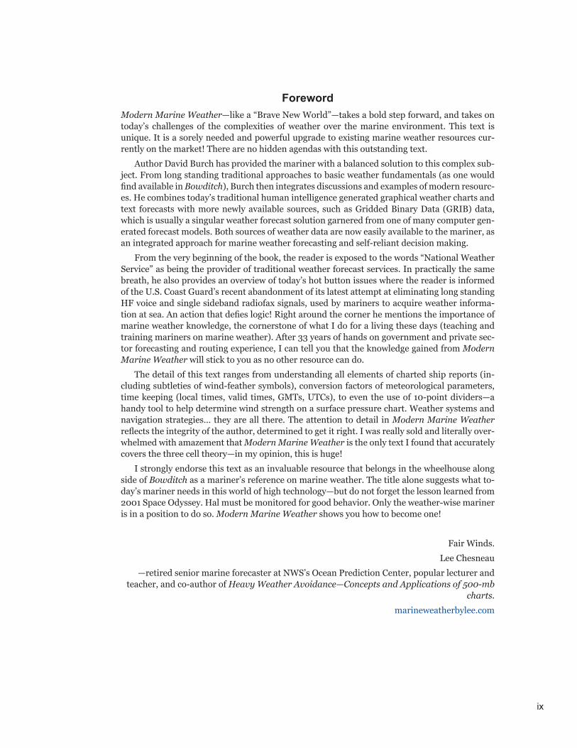
Foreword Modern Marine Weather—like a “Brave New World”—takes a bold step forward, and takes on today’s challenges of the complexities of weather over the marine environment. This text is unique. It is a sorely needed and powerful upgrade to existing marine weather resources cur-rently on the market! There are no hidden agendas with this outstanding text.

Author David Burch has provided the mariner with a balanced solution to this complex sub-ject. From long standing traditional approaches to basic weather fundamentals (as one would find available in Bowditch), Burch then integrates discussions and examples of modern resourc-es. He combines today’s traditional human intelligence generated graphical weather charts and text forecasts with more newly available sources, such as Gridded Binary Data (GRIB) data, which is usually a singular weather forecast solution garnered from one of many computer gen-erated forecast models. Both sources of weather data are now easily available to the mariner, as an integrated approach for marine weather forecasting and self-reliant decision making.

From the very beginning of the book, the reader is exposed to the words “National Weather Service” as being the provider of traditional weather forecast services. In practically the same breath, he also provides an overview of today’s hot button issues where the reader is informed of the U.S. Coast Guard’s recent abandonment of its latest attempt at eliminating long standing HF voice and single sideband radiofax signals, used by mariners to acquire weather informa-tion at sea. An action that defies logic! Right around the corner he mentions the importance of marine weather knowledge, the cornerstone of what I do for a living these days (teaching and training mariners on marine weather). After 33 years of hands on government and private sec-tor forecasting and routing experience, I can tell you that the knowledge gained from Modern Marine Weather will stick to you as no other resource can do.

The detail of this text ranges from understanding all elements of charted ship reports (in-cluding subtleties of wind-feather symbols), conversion factors of meteorological parameters, time keeping (local times, valid times, GMTs, UTCs), to even the use of 10-point dividers—a handy tool to help determine wind strength on a surface pressure chart. Weather systems and navigation strategies… they are all there. The attention to detail in Modern Marine Weather reflects the integrity of the author, determined to get it right. I was really sold and literally over-whelmed with amazement that Modern Marine Weather is the only text I found that accurately covers the three cell theory—in my opinion, this is huge!

I strongly endorse this text as an invaluable resource that belongs in the wheelhouse along side of Bowditch as a mariner’s reference on marine weather. The title alone suggests what to-day’s mariner needs in this world of high technology—but do not forget the lesson learned from 2001 Space Odyssey. Hal must be monitored for good behavior. Only the weather-wise mariner is in a position to do so. Modern Marine Weather shows you how to become one!

Fair Winds.Lee Chesneau

—retired senior marine forecaster at NWS’s Ocean Prediction Center, popular lecturer and teacher, and co-author of Heavy Weather Avoidance—Concepts and Applications of 500-mb

charts. marineweatherbylee.com

x

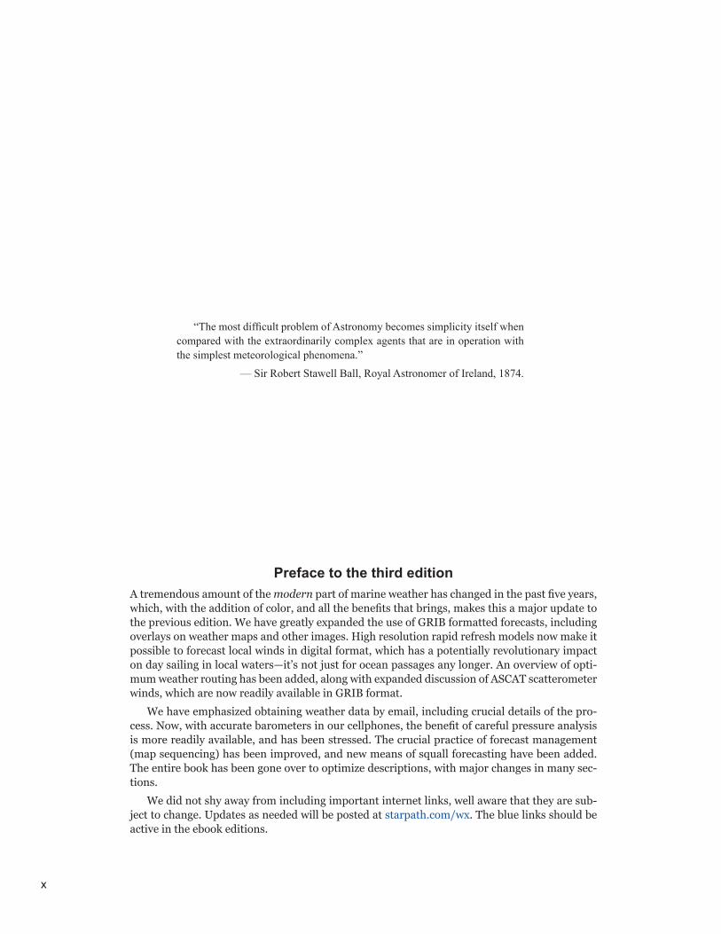
“The most difficult problem of Astronomy becomes simplicity itself when compared with the extraordinarily complex agents that are in operation with the simplest meteorological phenomena.”

— Sir Robert Stawell Ball, Royal Astronomer of Ireland, 1874.

Preface to the third editionA tremendous amount of the modern part of marine weather has changed in the past five years, which, with the addition of color, and all the benefits that brings, makes this a major update to the previous edition. We have greatly expanded the use of GRIB formatted forecasts, including overlays on weather maps and other images. High resolution rapid refresh models now make it possible to forecast local winds in digital format, which has a potentially revolutionary impact on day sailing in local waters—it’s not just for ocean passages any longer. An overview of opti-mum weather routing has been added, along with expanded discussion of ASCAT scatterometer winds, which are now readily available in GRIB format.

We have emphasized obtaining weather data by email, including crucial details of the pro-cess. Now, with accurate barometers in our cellphones, the benefit of careful pressure analysis is more readily available, and has been stressed. The crucial practice of forecast management (map sequencing) has been improved, and new means of squall forecasting have been added. The entire book has been gone over to optimize descriptions, with major changes in many sec-tions.

We did not shy away from including important internet links, well aware that they are sub-ject to change. Updates as needed will be posted at starpath.com/wx. The blue links should be active in the ebook editions.

1.1 OverviewWe admit immediately that Modern Marine Weather is a brave title. Of all technologies influencing marine navigation these days, those affecting weather preparation before a voy-age and analysis underway, are changing as fast as any—part-ly because products and services are evolving rapidly, but also because the related technologies of wireless communications are changing so fast as well. Monthly we have new sources and improved technologies related to marine weather. New services and products from the National Weather Service (NWS) and commercial companies appear frequently.

Most mariners know about text messaging by cellphone, but fewer know their phones can access wind speed, wind direction, and pressure at a buoy or lighthouse along their route, whenever they might want it. We can also use our phones to get a live radar view showing precise locations of squalls in our waters, updated every 6 seconds! Aircards and cellphone hotspots offer broadband connection to the inter-net in most inland waters and many near coastal waters. The number of phone and tablet apps for weather and navigation work is growing exponentially.

There is also ongoing research into fundamentals that are “windfalls” to our trade. The demand for new energy sources has spurred much research into wind power generation, in-cluding where to locate the generators and how they interact with each other and with the local terrain. This has led to in-depth study of wind flow over and around barricades, directly applicable to predicting how close we can sail to an islet 20 ft high versus one 80 ft high, and still maintain our wind. This is a valuable resource for knowledge on sailing near land. Ocean modeling continually improves with better sea state and ocean current forecasts.

If we are to keep this book’s title meaningful, we must stay on our toes and make every effort to keep the teaching mate-rials and presentations up to date. Traditional book publish-ing procedures have a challenge here. If a book takes a year in production, it is destined to be out of date when it arrives. We need new means of publication and teaching to keep up with the topic. The solution is pretty obvious. The internet is the main source of revolution in marine weather content and services, and it also provides the way to keep materials and information up to date. Of all topics in modern marine navi-gation, it is fair to say that weather is affected the most by the internet. Updates on the content of this book can be found at starpath.com/wx.

There are also good reasons to get involved with modern sources of marine weather. The United States Coast Guard (USCG) will eventually discontinue the traditional high fre-

quency (HF) broadcasts in voice and radiofax. In 2013 the middle frequency (MF) broadcasts were ended. High seas data in voice and radiofax—a longtime target for closing—are still available, but most sailors are already relying primarily on wireless connections to text versions of the reports and downloaded images of the weather maps. In contrast to the broadcasts, which are available at specific times only, these products can now be requested when needed by satellite phone (satphone) or HF radio. Check navcen.uscg.gov for the latest plans.

Needless to say, there are elements of weather work that do not change with time. What is changing are the types of data and how we receive them. What we do with the data in planning and navigation has not changed—what we watch in the sky and on the water, and how we choose our routes un-derway has not changed much since the great sailing days of the 1800’s—though we do sail to weather a lot better! There is much to learn from knowledge gained in those days, especial-ly from the works of pioneers such as Admiral Robert FitzRoy (1805-1865), the father of modern meteorology (and cap-tain of Darwin’s Beagle). We actually still use observations gathered by Captain Matthew Fontaine Maury (1806-1873) who compiled data from ship’s logs into the forerunners of modern Coast Pilots and Pilot Charts. We rely daily when un-derway on the Beaufort wind force scale of Admiral Francis Beaufort (1774-1857). Its value has not diminished. We also touch on the work of George Hadley (1685-1768) who initi-ated the understanding of what causes the trade wind flow, the doldrums, and the great mid-ocean Highs.

We still need these basics of weather observation and re-spect for the sea, long-tested in maritime tradition. Modern tools are blessings that must be used thoughtfully. Global Po-sitioning Systems (GPS), for example, has had a mixed influ-ence on the practice of marine navigation. Certainly it is now a most valuable aid to navigation—to the point that it is es-sentially negligent to navigate without it. But with the advent of its (usually) great accuracy and extreme convenience has come a tendency to not study the basics of navigation. When-ever our GPS fails or is unavailable, or we make a cockpit er-ror in using it, or when we are in some poorly charted area where having a digital position doesn’t help at all, we must fall back on the basics.

Likewise, in modern marine weather, there are new and wonderful resources available now that are analogous to the arrival of GPS. We can push buttons now and end up with a full weather map laid out on the electronic chart we are navi-gating with. The overlays even include wind arrows plotted

CHAPTER ONE

INTRODUCTION

MODERN MARINE WEATHER

2

on the chart, showing wind speed and direction everywhere around us. Push another button and the predicted wave heights and directions are plotted as well. Push another but-ton and we see how all of these change in the next hour, or the next day, or the next 5 days. We can obtain this data in a local bay or in the middle of the ocean. Just as when GPS was new, it is easy to ask, “Why do we need to study more?”

A main goal of this book is to answer that question. To ex-plain just what we are actually getting with such a push-but-ton system and how to use it safely. And of course to provide those basics we can fall back upon as needed. Continuing the GPS analogy, (which can tell us very nicely where we are, but does not tell us the best way to get to where we want to go) we also cover how to use the weather data we have, and how to interpret what we see around us in the water and sky. This helps to evaluate, and modify as needed, what we are told about the weather in order to choose the optimum course.

As for philosophy, a famous scientist once said that our goal in teaching practical science should be to make things as simple as possible—but not simpler. So a guiding principle has been to cover the theory of weather only insofar as it ac-tually helps us make decisions in planning and navigation. There are many excellent books on meteorology that cover the background in more depth. Selections are listed in the References. But there are some nuts and bolts we cannot skip if we want to best apply what we learn. Our goal is to make the text a practical guide to the acquisition, interpretation, and application of marine weather data—not just tell you about it, but tell you how to use it.

Which brings up a thought that occurs more than once in the book. There will always be a forecast, and they are not la-beled good or bad. At home we get 40% chance of rain, but at sea we do not get 40% chance of gale. So one of our ongoing goals underway and in our immediate planning of voyages is to develop those skills and resources that help us evaluate the forecasts we are given. We are not trying to outguess the professionals who gave us the forecast—that is not realistic. If they say the wind on the coast is going to be 20 kts, north of 38º 30’ N, at midday tomorrow, then, barring any immedi-ate contrary evidence, our best bet is to assume the wind is going to be 20 kts, north of 38º 30’ N, at midday tomorrow. They have more knowledge on the subject and they have far more data than what we can see around us or download from our wireless sources.

But we can evaluate the timing of what they forecast when we are located in the forecast region—or when we have access to measurements from the forecast region. Weather systems are in motion, and their route and speed may change. In the ocean, we may only hear from the professionals every 6 hrs or so—although there are exciting new sources on the horizon that will change that. It could be things have changed since their last report. With trained observational skills, we may be able to detect changes in the timing of the event before the next forecast. We may be able to conclude that this system is early, and we should look for that wind much earlier.

More to the point, however, with learned techniques and observations we can assign some level of confidence to the forecast. If our study indicates that all signs point to this be-ing a good forecast, then we carry on with more confidence. But, if our signs indicate this may not be such a good forecast, and if it is indeed wrong, our present plan may not be a good one. We are then better off just doing half of what we want to do, and wait for the next forecast to learn more.

In short, to do the best job with weather planning, we do not want to simply look at a map, read a text report, or listen to a voice broadcast, and say we are done—ready to make our decisions. Instead, we want to evaluate what we are told as carefully as possible. That evaluation process is another large part of the goal of this book.

Finally it might be valuable to point out early on that con-trary to some images of marine weather study, it is not all about bad weather. In fact, if we do our planning properly and use our resources properly, we will avoid bad weather most of the time. As sailors, we will use our knowledge far more often to find more wind than to avoid too much of it. Find a route with 14 kts instead of 10 kts and you will get there faster. Find one with 5 kts instead of 3 kts, and the ef-fect is even greater.

Practical knowledge of wind and waves is obviously not just the domain of sailors. The content of this book is equally valuable to all mariners. Just like the Navigation Rules, it applies to “every description of water craft used as a means of transportation on water.”

1.2 Role of Marine WeatherWhen putting out to sea for an extended passage, the first and foremost concern is a sound and well prepared boat; next comes the basic health, fitness, and seamanship of the crew. With these basics in place, next priorities are fundamental navigation skills and knowledge of marine weather. There are those who sail around the world with only the most rudimen-tary knowledge of weather at sea, but there is a great deal of luck involved in these cases, and probably more anxiety than necessary. More important to the conscientious voyager, there is usually more risk and inefficiency than need be.

Bad weather is always a test of boat and crew, but it more often affects the progress of a trip without necessarily threat-ening the safety of a well prepared boat. Although bad weath-er is always recalled more vividly than fair weather, gales and worse are not common occurrences in most cruising. Know-ing where and when bad weather is expected is fundamen-tal weather knowl edge every sailor should have. Avoiding it whenever possible is simply good seamanship. Weather sta-tistics are available in Coast Pilots and Sailing Directions, presented on Pilot Charts, and discussed in standard refer-ences such as Bowditch’s American Practical Navigator (nicknamed Bowditch). More detailed information can be found in the Mariner’s Weather Log, published online three times a year by NOAA. The Climatology of Global Ocean

MODERN MARINE WEATHER

8

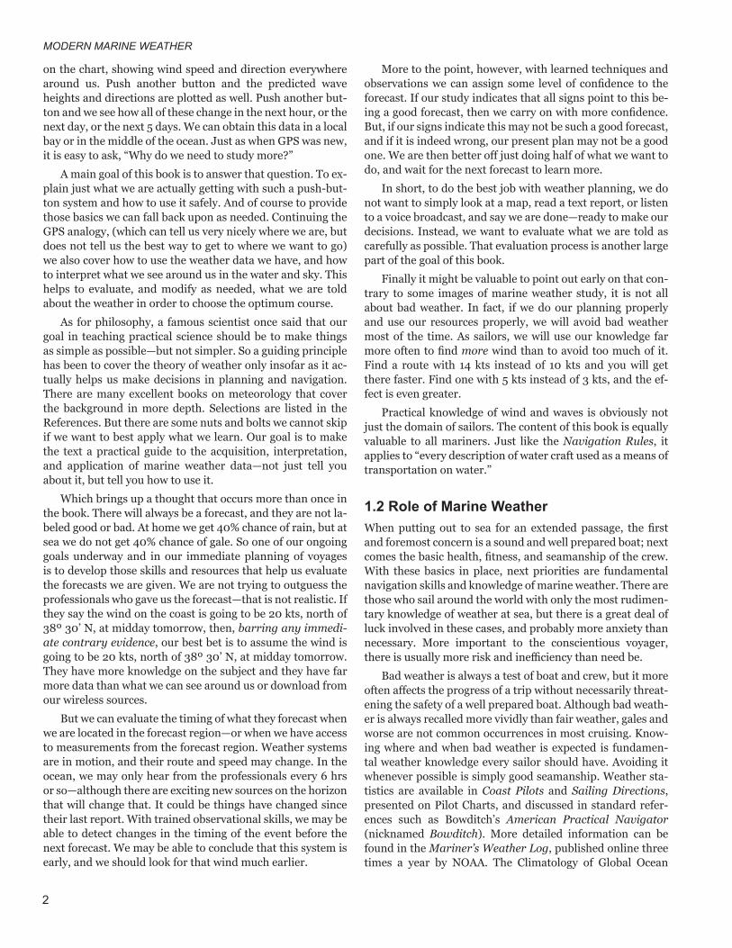
There are still more key terms related to the wind direc-tion. We have upwind and downwind, and windward and lee-ward. It is easy to overlook the distinction between these two sets of terms, but there is an important difference, which en-ters into official rules of sailing and of navigation in general.

Upwind and downwind are directions relative to a line perpendicular to the wind direction, whereas windward and leeward are directions relative to the centerline of the vessel. Windward and leeward are the opposite sides of the boat, un-less you are going exactly downwind, in which case the Navi-gation Rules define windward as “the side opposite to that on which the mainsail is carried...”

Upwind and downwind, in contrast, are defined by a line through your vessel that is perpendicular to true wind direc-tion. When you are tacking to weather with another vessel, that boat is ahead of you if he is upwind of you, regardless of where he is to windward or to leeward of you—and of course he can be ahead of you and to leeward. See Figure 1.5-5.

Moving on to symbols. Wind symbols are our starting point in reading weather maps. Figure 1.5-6 is an actual graphic definition given on an official NWS web site.

It shows the basic idea: half a feather is 5 kts; full is 10; a flag is 50. The arrow flows in the direction of the wind. Five knots is displaced from the end so as not to be confused with 10 kts. But other than those basics, this is a pretty poor defin-ing graphic. First the winds marked NE are not from the NE according to these arrows; they vary from 014 to 024. If these were NE winds they should be oriented toward 045. The one labeled NNE shown at 008 is also wrong, it should be halfway between 000 and 045. Wind directions shown on maps and discussed in conversations and in writing are always assumed to be true directions unless specifically stated otherwise.

Secondly, the winds indicated in that defining graphic are not really what these symbols mean, though often stated that way. An arrow flowing from the NE with 1 feather means the wind at the arrow tip is anywhere between 7.5 kts and 12.5 kts. It does not mean the wind is specifically 10 kts. The force of the wind varies as the square of the wind speed, so 12.5 kts of wind is about 3 times “stronger” than that of 7.5 kts (12.5 × 12.5 ÷ 7.5 × 7.5 = 2.8). Likewise, one and a half feathers means winds of anywhere from 12.5 to 17.5 kts, spanning a factor of 2 in wind force. (See illustration opposite the title page.)

With this in mind, sailors would like to know forecasted wind speeds as accurately as possible, and indeed the predic-tions will be more precise than ± 2.5 kts. This does not mean the forecasts will be that accurate, but we certainly do not want to throw away precision that might be right.

Concern for these details is definitely a reflection on modern resources available. Standard weather maps gener-ated by various weather offices around the world display the wind in this rounded format because (at least historically) they probably do not believe they were more accurate than that. And that is fair enough. But the NWS surface analysis maps that we use plot the actual ship reports of the wind, and these reports are received typically to a precision of ±0.5 kts (rounded to whole knots) and directions rounded to 10º.

Some years ago, all the winds in the world were typically reported as N, NE, E, SE, etc., at 15, 20, 25 kts, etc. But the Port Meteorological Officers (PMOs) at the NWS who coor-dinate the Vessel Observing Ship (VOS) program have done a good job over the years training the ship’s officers who turn in the weather observations. Now we get more precise ob-servations, corrected for vessel motion. We also now have satellite wind measurements that help identify actual winds on the ocean surface. Taking into account known limitations, accuracy standards for observations (human and satellite) are about ±2 kts in speed and ±20º in direction, but with

Figure 1.5-5. Upwind - downwind; windward - leeward.

Figure 1.5-6. Wind arrows from an official online source—an ex-ample of the sometimes poor definitions we run across.

NE 2 KT NE 5 KT NE 10 KT NE 15 KT NNE 45 KT N 50 KT N 65 KT

Upwind

Downwind

Windward

Leeward

Upwind

Downwind

Windward

Leeward

Figure 1.5-7. Wind vectors near the Equator (Galapagos Islands), showing the convention of drawing the feathers on opposite sides of the arrow in the Northern and Southern Hemispheres. We get a better insight into this convention later on—the feathers are always on the low-pressure side of the wind direction, which is a reminder of what is called Buys Ballot’s Law. Remember, too, in cases like this where the wind feathers span some 40 miles at this scale, that the report location is at the tip of the arrow.

Equator

MODERN MARINE WEATHER

10

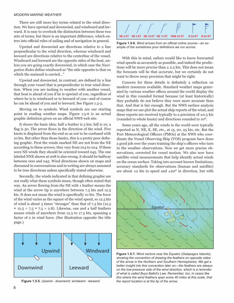
1.6-3—a ship report plotted as a nominal 20 kts (2 feathers) from the NNW. If we cared to study this map in depth, we could actually send an email request for the exact reports that it shows. A sample of such reports is shown in Table 1.6-1 be-low the figure. We see that this symbol plotted as a nominal 20 kts was actually 22 kts with a reported direction of 330 T.

Comparing the other samples, we see the reports and symbols are all fairly consistent with the map—except report “A,” which clearly had a wrong pressure (report of 1030.2 when located just inside the 1024 isobar), but this type of dis-crepancy is rare. That wind report is also not consistent with the map, as we will understand better later in the book. We address maps and isobars throughout the book as we pro-ceed; for now we are just looking at the use of wind symbols.

Another topic worth introducing early that we shall come back to in depth, is the use of vector wind forecasts in GRIB (GRIdded Binary) format. This system of GRIB data sources and GRIB data viewers is a primary tool for modern weather work. Working with GRIB forecasts as soon as possible not

only helps with learning the basics behind them, it also puts live weather data in your hands at the same time.

Surface analysis and forecast maps provided by the NWS are often based on the Global Forecast System (GFS) numeri-cal weather prediction model (discussed later). Mariners have ubiquitous access to GFS model data that the NWS uses, which provide wind and pressure forecasts every 6 hrs out to ten days, the first three or four of which can be fairly reli-able. Most navigation software programs we use underway provide a way to request the data wirelessly worldwide, as well as a means of displaying it.

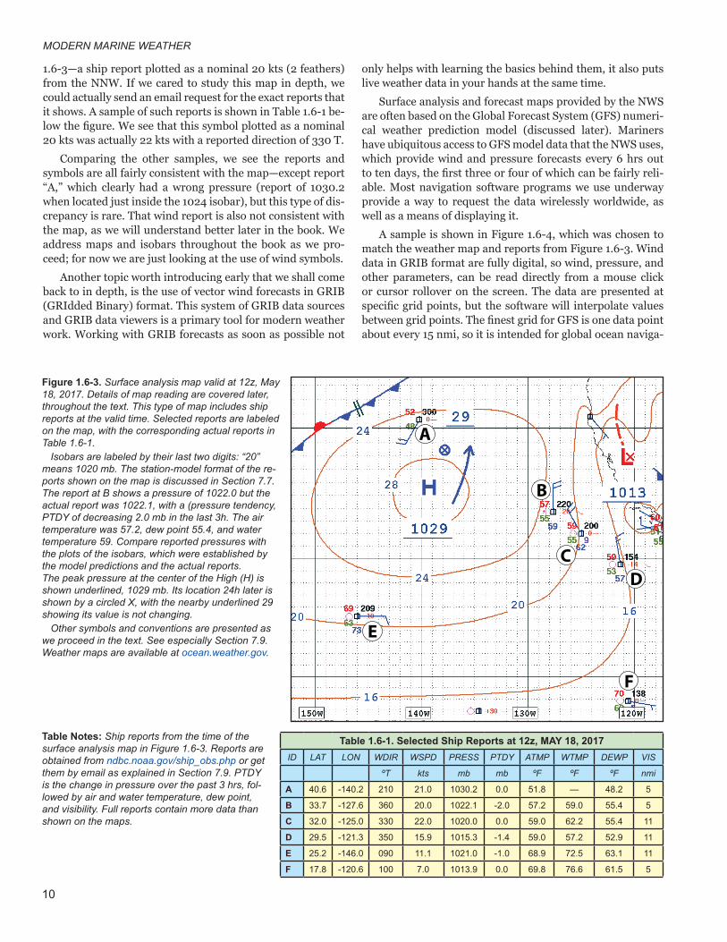
A sample is shown in Figure 1.6-4, which was chosen to match the weather map and reports from Figure 1.6-3. Wind data in GRIB format are fully digital, so wind, pressure, and other parameters, can be read directly from a mouse click or cursor rollover on the screen. The data are presented at specific grid points, but the software will interpolate values between grid points. The finest grid for GFS is one data point about every 15 nmi, so it is intended for global ocean naviga-

Table 1.6-1. Selected Ship Reports at 12z, MAY 18, 2017 ID LAT LON WDIR WSPD PRESS PTDY ATMP WTMP DEWP VIS

ºT kts mb mb ºF ºF ºF nmi

A 40.6 -140.2 210 21.0 1030.2 0.0 51.8 — 48.2 5

B 33.7 -127.6 360 20.0 1022.1 -2.0 57.2 59.0 55.4 5

C 32.0 -125.0 330 22.0 1020.0 0.0 59.0 62.2 55.4 11

D 29.5 -121.3 350 15.9 1015.3 -1.4 59.0 57.2 52.9 11

E 25.2 -146.0 090 11.1 1021.0 -1.0 68.9 72.5 63.1 11

F 17.8 -120.6 100 7.0 1013.9 0.0 69.8 76.6 61.5 5

Figure 1.6-3. Surface analysis map valid at 12z, May 18, 2017. Details of map reading are covered later, throughout the text. This type of map includes ship reports at the valid time. Selected reports are labeled on the map, with the corresponding actual reports in Table 1.6-1.

Isobars are labeled by their last two digits: “20” means 1020 mb. The station-model format of the re-ports shown on the map is discussed in Section 7.7. The report at B shows a pressure of 1022.0 but the actual report was 1022.1, with a (pressure tendency, PTDY of decreasing 2.0 mb in the last 3h. The air temperature was 57.2, dew point 55.4, and water temperature 59. Compare reported pressures with the plots of the isobars, which were established by the model predictions and the actual reports. The peak pressure at the center of the High (H) is shown underlined, 1029 mb. Its location 24h later is shown by a circled X, with the nearby underlined 29 showing its value is not changing.

Other symbols and conventions are presented as we proceed in the text. See especially Section 7.9. Weather maps are available at ocean.weather.gov.

Table Notes: Ship reports from the time of the surface analysis map in Figure 1.6-3. Reports are obtained from ndbc.noaa.gov/ship_obs.php or get them by email as explained in Section 7.9. PTDY is the change in pressure over the past 3 hrs, fol-lowed by air and water temperature, dew point, and visibility. Full reports contain more data than shown on the maps.

A

B

CD

E

F

CHAPTER 1. INTRODUCTION

11

A

B

C

D

28

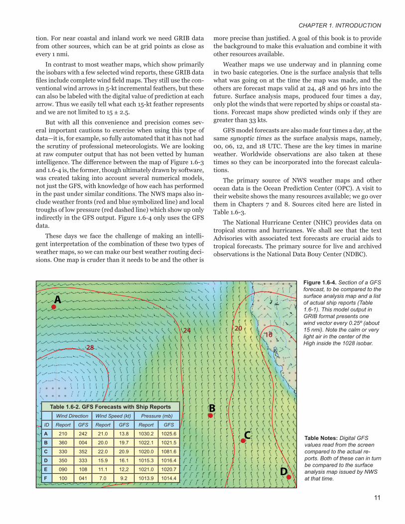
24 2016

Figure 1.6-4. Section of a GFS forecast, to be compared to the surface analysis map and a list of actual ship reports (Table 1.6-1). This model output in GRIB format presents one wind vector every 0.25º (about 15 nmi). Note the calm or very light air in the center of the High inside the 1028 isobar.

Table 1.6-2. GFS Forecasts with Ship ReportsWind Direction Wind Speed (kt) Pressure (mb)

ID Report GFS Report GFS Report GFS

A 210 242 21.0 13.8 1030.2 1025.6

B 360 004 20.0 19.7 1022.1 1021.5

C 330 352 22.0 20.9 1020.0 1081.6

D 350 333 15.9 16.1 1015.3 1016.4

E 090 108 11.1 12,2 1021.0 1020.7

F 100 041 7.0 9.2 1013.9 1014.4

tion. For near coastal and inland work we need GRIB data from other sources, which can be at grid points as close as every 1 nmi.

In contrast to most weather maps, which show primarily the isobars with a few selected wind reports, these GRIB data files include complete wind field maps. They still use the con-ventional wind arrows in 5-kt incremental feathers, but these can also be labeled with the digital value of prediction at each arrow. Thus we easily tell what each 15-kt feather represents and we are not limited to 15 ± 2.5.

But with all this convenience and precision comes sev-eral important cautions to exercise when using this type of data—it is, for example, so fully automated that it has not had the scrutiny of professional meteorologists. We are looking at raw computer output that has not been vetted by human intelligence. The difference between the map of Figure 1.6-3 and 1.6-4 is, the former, though ultimately drawn by software, was created taking into account several numerical models, not just the GFS, with knowledge of how each has performed in the past under similar conditions. The NWS maps also in-clude weather fronts (red and blue symbolized line) and local troughs of low pressure (red dashed line) which show up only indirectly in the GFS output. Figure 1.6-4 only uses the GFS data.

These days we face the challenge of making an intelli-gent interpretation of the combination of these two types of weather maps, so we can make our best weather routing deci-sions. One map is cruder than it needs to be and the other is

more precise than justified. A goal of this book is to provide the background to make this evaluation and combine it with other resources available.

Weather maps we use underway and in planning come in two basic categories. One is the surface analysis that tells what was going on at the time the map was made, and the others are forecast maps valid at 24, 48 and 96 hrs into the future. Surface analysis maps, produced four times a day, only plot the winds that were reported by ships or coastal sta-tions. Forecast maps show predicted winds only if they are greater than 33 kts.

GFS model forecasts are also made four times a day, at the same synoptic times as the surface analysis maps, namely, 00, 06, 12, and 18 UTC. These are the key times in marine weather. Worldwide observations are also taken at these times so they can be incorporated into the forecast calcula-tions.

The primary source of NWS weather maps and other ocean data is the Ocean Prediction Center (OPC). A visit to their website shows the many resources available; we go over them in Chapters 7 and 8. Sources cited here are listed in Table 1.6-3.

The National Hurricane Center (NHC) provides data on tropical storms and hurricanes. We shall see that the text Advisories with associated text forecasts are crucial aids to tropical forecasts. The primary source for live and archived observations is the National Data Bouy Center (NDBC).

Table Notes: Digital GFS values read from the screen compared to the actual re-ports. Both of these can in turn be compared to the surface analysis map issued by NWS at that time.

MODERN MARINE WEATHER

12

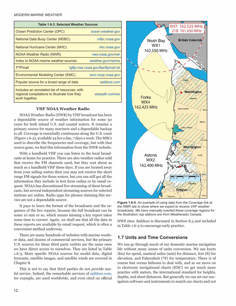
VHF NOAA Weather RadioNOAA Weather Radio (NWR) by VHF broadcast has been

a dependable source of weather information for some 50 years for both inland U.S. and coastal waters. It remains a primary source for many mariners and a dependable backup to all. Coverage is essentially continuous along the U.S. coast (Figure 1.6-5), available 24 hrs a day, 7 days a week. The MSCs used to describe the frequencies and coverage, but with that source gone, we find this information from the NWR website.

With a handheld VHF you can listen to the local broad-casts at home for practice. There are also weather radios sold that receive the FM channels used, but they cost about as much as a handheld VHF these days. If you are located away from your sailing waters then you may not receive the short range FM signals for those waters, but you can still get all the information they include in text form online or by email re-quest. NOAA has discontinued live streaming of these broad-casts, but several independent streaming sources for selected stations are online. Radio apps for phones claiming this ser-vice are not a dependable source.

It pays to learn the format of the broadcasts and the se-quence of the live reports, because the full broadcast can be some 10 min or so, which means missing a key report takes some time to correct. Again, we shall see that all the data in these reports are available by email request, which is often a convenient method underway.

There are many hundreds of websites with marine weath-er data, and dozens of commercial services, but the primary U.S. sources for these third party outlets are the same ones we have direct access to ourselves. They are listed in Table 1.6-3. More specific NOAA sources for model data, digital forecasts, satellite images, and satellite winds are covered in Chapter 8.

This is not to say that third parties do not provide use-ful service. Indeed, the remarkable services of saildocs.com, for example, are used worldwide, and even cited on official

NWS sites. Saildocs is discussed in Section 8.3 and included in Table 1.6-3 to encourage early practice.

1.7 Units and Time ConversionsWe can go through much of our domestic marine navigation life without many issues of units conversion. We use knots (kts) for speed, nautical miles (nmi) for distance, feet (ft) for elevation, and Fahrenheit (ºF) for temperature. There is of course feet versus fathoms to deal with, and as we move on to electronic navigational charts (ENC) we get much more practice with meters, the international standard for heights, depths, and short distances. But generally we can set our nav-igation software and instruments to match our charts and not

162.550 MHz

162.425 MHz

WX7 162.525 MHz21B 161.650 MHz

162.400 MHz

Figure 1.6-5. An example of using data from the Coverage link at the NWR site to show where we expect to receive VHF weather broadcasts. We have manually overlaid these coverage regions for the illustration; top stations are from Weatheradio Canada.

Table 1.6-3. Selected Weather Sources

Ocean Prediction Center (OPC) ocean.weather.gov

National Data Buoy Center (NDBC) ndbc.noaa.gov

National Hurricane Center (NHC) nhc.noaa.gov

NOAA Weather Radio (NWR) nws.noaa.gov/nwr

Index to NOAA marine weather sources weather.gov/marine

FTPmail tgftp.nws.noaa.gov/fax/ftpmail.txt

Environmental Modeling Center (EMC) emc.ncep.noaa.gov

Popular source for a broad range of data saildocs.com

Includes an annotated list of resources, with regional compilations to illustrate how they work together.

starpath.com/wx

MODERN MARINE WEATHER

14

TimekeepingAnd then there is timekeeping—local time versus Green-

wich Mean Time (GMT), now called Universal Coordinated Time (UTC); valid times versus broadcast times on weather maps; watch times versus zone times; and so on. Weather work requires more care in timekeeping than any other area of navigation, including celestial navigation, which has a lot of focus on timekeeping.

Don’t be surprised to find this a challenge when you begin work in marine weather—and it is, of course, crucial that it be done right. This will call for a whole section on sequencing of forecasts in Chapter 7, but for now we provide a preview of some issues involved.

First, all weather maps and many (not all) text forecasts are given in coordinated universal time (UTC), which is also called by some agencies universal time (UT), though there is technically a difference. This has been the proper name of Greenwich Mean Time (GMT) for quite a few years now, but we still see GMT used on some weather products. There is interesting history on how this name change came about, but this not significant to our subject.

UTC is often abbreviated with the letter “z” (zulu), be-cause every zone in the zone-time system was at one time as-signed a letter label, and “z” is the label for time zone zero. The synoptic times are therefore often listed as 00z, 06z, 12z, and 18z. In modern times, letter labels are not used for the other time zones. Again, there is interesting history behind these labels—they skipped the letter “j” for example—but we leave this for a Wikipedia project.

In marine navigation time zones are defined by their zone description (ZD), such that UTC = zone time + ZD. (This also applies to standard times and daylight times.) Pacific Daylight Time (PDT), for example, has a ZD of +7h. Suppose it is 2125 PDT on May 29. When we look at the ra-diofacsimile broadcast schedule online (ocean.weather.gov/ fax_schedules.shtml), we see that available maps are sorted by their HF radio broadcast times, in UTC, labeled with a “z.” At present, UTC = 2125 + 7 = 2825 = 0425z on May 30, and the schedule shows the most recent surface analysis map for the Eastern Pacific was available at 0331z, and that it is valid for 00z, on May 30. When we download and print out that map it will say that it is, “VALID: 00:00 UTC 30 MAY” which was 1700 PDT on May 29. The same time that is labeled “z” on the schedule is labeled UTC on the map.

Thus at the present time (2125 PDT), the most recent map available was valid for 1700 PDT, which is 4h 25m old. This is not quite as bad as it looks, because the earliest we could have got it was 0331z, so this map is already 3h 31m old at birth. It takes that long to compile all the ooz observations worldwide, feed them into a computer, get out the forecast, process it, and distribute it. Remember that 00:00 UTC is the first mo-ment of the day, which is the same as 24:00 of the previous day, if we need to add or subtract times.

At this point we could look ahead on the schedule to see when the next analysis (06z) will be available. The answer is 0919z, which will be 0219 PDT tomorrow, or 4h 54m from now. This map will be 3h 19m old at birth. The times we can download the maps compared to the times they are broadcast vary with the maps. Some downloads are available earlier, some later. The relative age of the maps at birth vary from one map type to the next, but for specific map types they re-main about the same.

When it comes to comparing the 00z analysis to our own observations, we have to look in our logbook for our recorded position, wind speed, wind direction, and pressure records at the valid map time, 00z, which would have been 1700 PDT today, 4h 25m ago. We learn quickly that it is crucial to make a log entry at the synoptic times with position, wind, and pressure data.

In short, we have no way around reckoning times forward and backward multiple times each day in different time sys-tems. When we add to this forecast maps, which are avail-able at different times still, and valid in the future not the past, things just get worse. And there are no shortcuts, such as choosing to work only in UTC. Everyone else on the vessel is working on ship’s time, which is only fair. This nastiness is best kept in the nav station.

The trick is just go slow and label maps or printed reports with the ship’s time. It will always be helpful on long pas-sages to make up a time schedule of when various products are available and when they are valid. We have samples in Chapter 7 on map reading, where we also propose ways to store and organize weather maps. It is valuable to keep all the weather broadcasts on the same printed schedule: voice, text, and maps.

Also in these modern times, it is likely that you are not relying on HF radiofax broadcasts for these products, but are rather downloading them by satellite telephone or HF radio connected to a Pactor modem (Chapter 8). This has the big advantage of requesting the products when you want to, rath-er than having to listen to the live broadcasts at specific times, but we still have to know when they are first available, so the custom-made time schedule is still important. In fact, it is even more important, because many of the satphone weather services (such as GRIB data and compressed weather maps) add an extra time delay to the product distribution to account for the time it takes them to collect the data from the NWS and process them. This adds another column to our custom broadcast schedule.

2.1 What Makes the WindIn Chapter 1 we learned the importance of wind in marine weather; now we take a closer look at wind and what causes it. The more we know about the forces that drive the wind, the better prepared we are to understand what is going on and make educated guesses at what might happen next.

Away from several important influences of land, the wind speed and direction we might anticipate (forecast) depends on where we happen to stand within a particular atmospher-ic pressure pattern. But knowledge builds upon itself. Often times, the best indicator of where we are in a pressure pat-tern is the actual direction of the present wind, and how this direction is changing with time. To understand this requires an understanding of how wind flows around high and low pressure systems, which we will get to after a review of at-mospheric pressure itself. In the next section we cover the important use of barometers for reading the pressure when underway.

A 10-kt wind means the air—or a balloon riding along in this air—moves 10 nmi in 1 hr. Air is a fluid with mass, just as water is, although air is some 800 times lighter (less dense) than water and much more compressible.

Understanding the fluid nature of air and its interaction with fluid water and water vapor is helpful in describing much of practical marine weather. The fluid-fluid interaction between surface winds and the sea makes waves in the sea; a similar interaction between high-altitude winds and the water vapor of clouds makes waves in the clouds. Prominent cloud waves show the direction of the winds aloft just as well as water waves show the direction of surface winds—the direc-tion of the winds aloft is extremely valuable to know, because it tells us the direction that storms move. Also, storms and frontal systems in the atmosphere behave much like eddies in rivers and waves in the ocean. We cover this in Chapter 3.

Air is held to the earth by gravity; if the earth were not heavy enough to provide this attraction, the air would spin off into space from the outward centrifugal force caused by the earth’s rotation. Because air is compressible and the holding power of gravity decreases with increasing altitude, most of the atmosphere is compressed into a thin layer at the earth’s surface, and this layer becomes less dense with increasing al-titude above the surface.

Roughly 80 percent of the air is below 40,000 feet, with some 50 percent of the air below 18,000 feet. This altitude, which marks the halfway point through the atmosphere, is an important demarcation line in meteorology, because most of the atmospheric disturbances we experience as weather on the surface are confined to this first 18,000 feet of air. The

winds above this altitude are stronger and much more per-sistent than those of the surface; also, the nature of clouds changes—from water vapor to ice crystals—at roughly this altitude.

Besides growing less dense with increasing altitude, the air also grows colder with altitude as less and less of the “at-mospheric blanket” is above it to keep it warm. As a rough average, the air temperature drops about 4 Fº per 1,000 feet of altitude as you rise through the atmosphere. Distinct cloud bases (ceilings) occur at the altitude at which the air tempera-ture has dropped to the dew point of the air.

Although air weighs very little per unit volume, the total weights involved are still impressive. A typical room contains about 100 pounds of air. Over each square mile of the earth’s surface there is some 30 million tons of air, and these massive amounts of air are not uniformly distributed over the surface. An uneven distribution of air is what causes the wind. If air flows across an entire state, for example, from the north at 20 kts, all day long, then there must have been very much more air to the north than there was to the south.

The amount of air at any place is determined by measuring the atmospheric pressure at that place. One way to describe atmospheric pressure is to simply state how much the air weighs that stands above a given area; a typical value would be 14.7 pounds per square inch, meaning a column of air, one square inch across, extending from the surface straight up to the top of the atmosphere weighs about 14.7 pounds. This is a perfectly valid unit of pressure, but it is more convenient and conventional for tires and scuba tank pressures than for at-mospheric pressures—in these units, atmospheric pressures typically vary between 14.4 and 14.8 pounds per square inch.

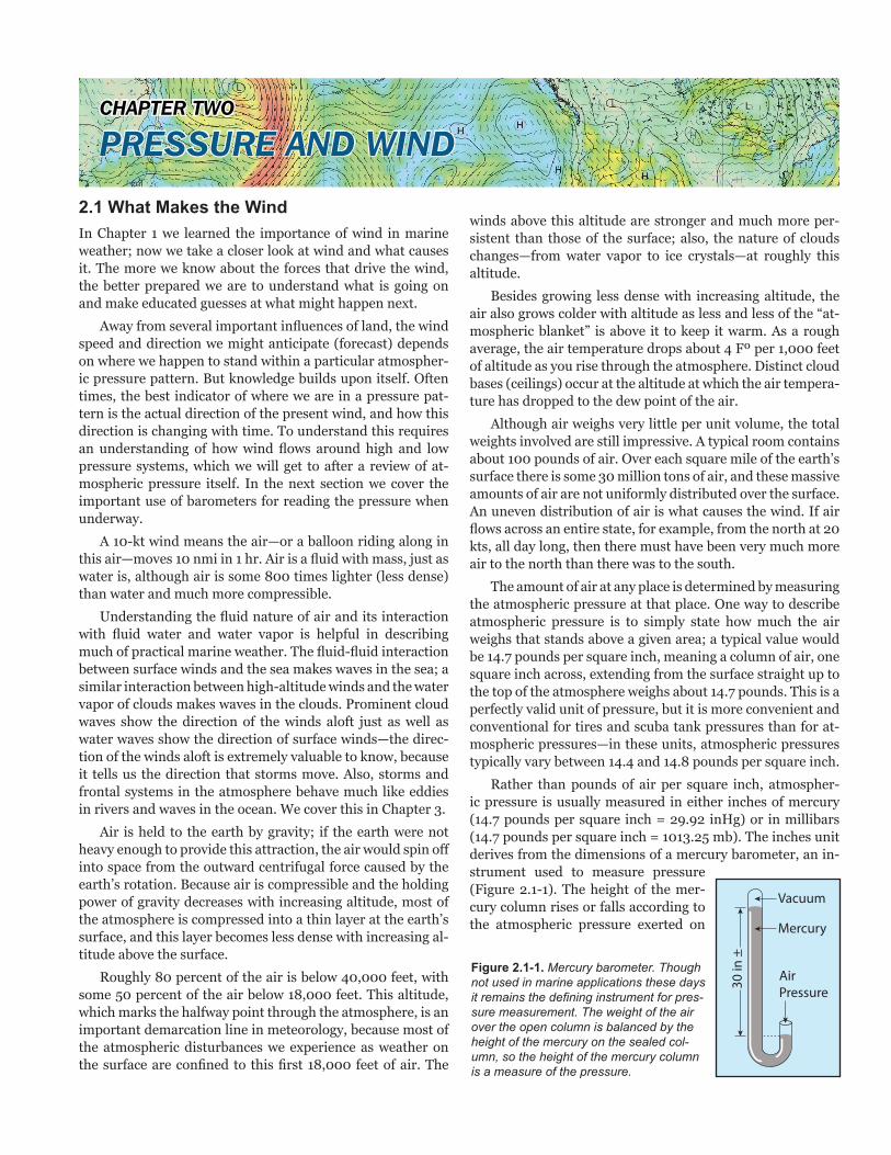
Rather than pounds of air per square inch, atmospher-ic pressure is usually measured in either inches of mercury (14.7 pounds per square inch = 29.92 inHg) or in millibars (14.7 pounds per square inch = 1013.25 mb). The inches unit derives from the dimensions of a mercury barometer, an in-strument used to measure pressure (Figure 2.1-1). The height of the mer-cury column rises or falls according to the atmospheric pressure exerted on

Figure 2.1-1. Mercury barometer. Though not used in marine applications these days it remains the defining instrument for pres-sure measurement. The weight of the air over the open column is balanced by the height of the mercury on the sealed col-umn, so the height of the mercury column is a measure of the pressure.

CHAPTER TWO

PRESSURE AND WIND

Vacuum

Mercury

Air Pressure30

in ±

CHAPTER 3. GLOBAL WINDS AND CURRENTS

75

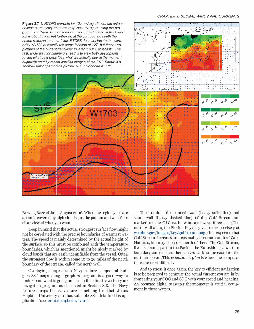
Figure 3.7-4. RTOFS currents for 12z on Aug 15 overlaid onto a section of the Navy Features map issued Aug 15 using the pro-gram Expedition. Cursor scans shows current speed in the lower left is about 4 kts, but farther on at the curve to the south the speed reduces to about 2 kts. RTOFS does not locate the warm eddy W1703 at exactly the same location at 12Z, but these two pictures of the current get closer in later RTOFS forecasts. The task underway for planning ahead is to view both descriptions to see what best describes what we actually see at the moment, supplemented by recent satellite images of the SST. Below is a zoomed few of part of the picture. SST color code is in ºF.

Rowing Race of June-August 2006. When the region you care about is covered by high clouds, just be patient and wait for a clear view of what you want.

Keep in mind that the actual strongest surface flow might not be correlated with the precise boundaries of warmest wa-ters. The speed is mainly determined by the actual height of the surface, so this must be combined with the temperature boundaries, which as mentioned might be nicely marked by cloud bands that are easily identifiable from the vessel. Often the strongest flow is within some 10 to 30 miles of the north boundary of the stream, called the north wall.

Overlaying images from Navy features maps and Rut-gers SST maps using a graphics program is a good way to understand what is going on—or do this directly within your navigation program as discussed in Section 8.8. The Navy features maps themselves are something like that. Johns Hopkins University also has valuable SST data for this ap-plication (see fermi.jhuapl.edu/avhrr).

The location of the north wall (heavy solid line) and south wall (heavy dashed line) of the Gulf Stream are marked on the OPC 24-hr wind and wave forecasts. (The north wall along the Florida Keys is given more precisely at weather.gov/images/key/gulfstream.png.) It is expected that Gulf Stream forecasts are reasonably accurate south of Cape Hatteras, but may be less so north of there. The Gulf Stream, like its counterpart in the Pacific, the Kuroshio, is a western boundary current that then curves back to the east into the northern ocean. This extension region is where the computa-tions are most difficult.

And to stress it once again, the key to efficient navigation is to be prepared to compute the actual current you are in by comparing your COG and SOG with your speed and heading. An accurate digital seawater thermometer is crucial equip-ment in these waters.

52 - 5454 - 56

56 - 5858 - 60

60 - 6262 - 64

64 - 6666 - 68

68 - 7070 - 72

72 - 7474 - 76

76 - 7878 - 80

80 - 8282 - 84

MODERN MARINE WEATHER

76

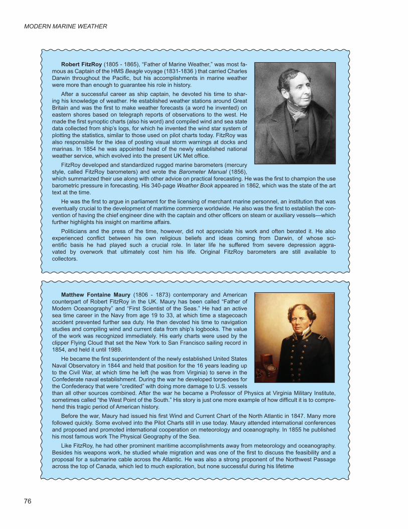
Robert FitzRoy (1805 - 1865), “Father of Marine Weather,” was most fa-mous as Captain of the HMS Beagle voyage (1831-1836 ) that carried Charles Darwin throughout the Pacific, but his accomplishments in marine weather were more than enough to guarantee his role in history.

After a successful career as ship captain, he devoted his time to shar-ing his knowledge of weather. He established weather stations around Great Britain and was the first to make weather forecasts (a word he invented) on eastern shores based on telegraph reports of observations to the west. He made the first synoptic charts (also his word) and compiled wind and sea state data collected from ship’s logs, for which he invented the wind star system of plotting the statistics, similar to those used on pilot charts today. FitzRoy was also responsible for the idea of posting visual storm warnings at docks and marinas. In 1854 he was appointed head of the newly established national weather service, which evolved into the present UK Met office.

FitzRoy developed and standardized rugged marine barometers (mercury style, called FitzRoy barometers) and wrote the Barometer Manual (1856), which summarized their use along with other advice on practical forecasting. He was the first to champion the use barometric pressure in forecasting. His 340-page Weather Book appeared in 1862, which was the state of the art text at the time.

He was the first to argue in parliament for the licensing of merchant marine personnel, an institution that was eventually crucial to the development of maritime commerce worldwide. He also was the first to establish the con-vention of having the chief engineer dine with the captain and other officers on steam or auxiliary vessels—which further highlights his insight on maritime affairs.

Politicians and the press of the time, however, did not appreciate his work and often berated it. He also experienced conflict between his own religious beliefs and ideas coming from Darwin, of whose sci-entific basis he had played such a crucial role. In later life he suffered from severe depression aggra-vated by overwork that ultimately cost him his life. Original FitzRoy barometers are still available to collectors.

Matthew Fontaine Maury (1806 - 1873) contemporary and American counterpart of Robert FitzRoy in the UK. Maury has been called “Father of Modern Oceanography” and “First Scientist of the Seas.” He had an active sea time career in the Navy from age 19 to 33, at which time a stagecoach accident prevented further sea duty. He then devoted his time to navigation studies and compiling wind and current data from ship’s logbooks. The value of the work was recognized immediately. His early charts were used by the clipper Flying Cloud that set the New York to San Francisco sailing record in 1854, and held it until 1989.

He became the first superintendent of the newly established United States Naval Observatory in 1844 and held that position for the 16 years leading up to the Civil War, at which time he left (he was from Virginia) to serve in the Confederate naval establishment. During the war he developed torpedoes for the Confederacy that were “credited” with doing more damage to U.S. vessels than all other sources combined. After the war he became a Professor of Physics at Virginia Military Institute, sometimes called “the West Point of the South.” His story is just one more example of how difficult it is to compre-hend this tragic period of American history.

Before the war, Maury had issued his first Wind and Current Chart of the North Atlantic in 1847. Many more followed quickly. Some evolved into the Pilot Charts still in use today. Maury attended international conferences and proposed and promoted international cooperation on meteorology and oceanography. In 1855 he published his most famous work The Physical Geography of the Sea.

Like FitzRoy, he had other prominent maritime accomplishments away from meteorology and oceanography. Besides his weapons work, he studied whale migration and was one of the first to discuss the feasibility and a proposal for a submarine cable across the Atlantic. He was also a strong proponent of the Northwest Passage across the top of Canada, which led to much exploration, but none successful during his lifetime

CHAPTER 4. STRONG WIND SYSTEMS

83

C

D

E

AB

03:58

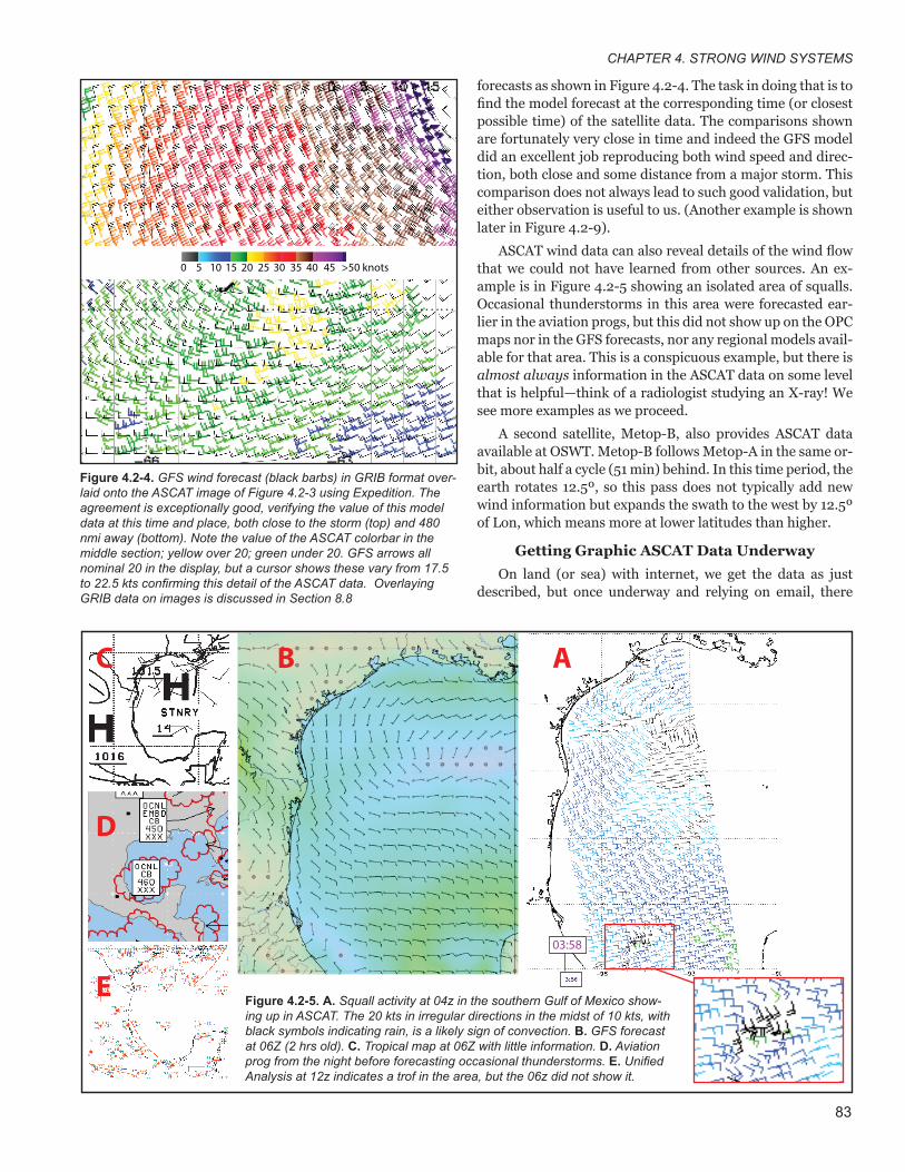
Figure 4.2-4. GFS wind forecast (black barbs) in GRIB format over-laid onto the ASCAT image of Figure 4.2-3 using Expedition. The agreement is exceptionally good, verifying the value of this model data at this time and place, both close to the storm (top) and 480 nmi away (bottom). Note the value of the ASCAT colorbar in the middle section; yellow over 20; green under 20. GFS arrows all nominal 20 in the display, but a cursor shows these vary from 17.5 to 22.5 kts confirming this detail of the ASCAT data. Overlaying GRIB data on images is discussed in Section 8.8

forecasts as shown in Figure 4.2-4. The task in doing that is to find the model forecast at the corresponding time (or closest possible time) of the satellite data. The comparisons shown are fortunately very close in time and indeed the GFS model did an excellent job reproducing both wind speed and direc-tion, both close and some distance from a major storm. This comparison does not always lead to such good validation, but either observation is useful to us. (Another example is shown later in Figure 4.2-9).

ASCAT wind data can also reveal details of the wind flow that we could not have learned from other sources. An ex-ample is in Figure 4.2-5 showing an isolated area of squalls. Occasional thunderstorms in this area were forecasted ear-lier in the aviation progs, but this did not show up on the OPC maps nor in the GFS forecasts, nor any regional models avail-able for that area. This is a conspicuous example, but there is almost always information in the ASCAT data on some level that is helpful—think of a radiologist studying an X-ray! We see more examples as we proceed.

A second satellite, Metop-B, also provides ASCAT data available at OSWT. Metop-B follows Metop-A in the same or-bit, about half a cycle (51 min) behind. In this time period, the earth rotates 12.5º, so this pass does not typically add new wind information but expands the swath to the west by 12.5º of Lon, which means more at lower latitudes than higher.

Getting Graphic ASCAT Data UnderwayOn land (or sea) with internet, we get the data as just

described, but once underway and relying on email, there

0 5 10 15 20 25 30 35 40 45 >50 knots

Figure 4.2-5. A. Squall activity at 04z in the southern Gulf of Mexico show-ing up in ASCAT. The 20 kts in irregular directions in the midst of 10 kts, with black symbols indicating rain, is a likely sign of convection. B. GFS forecast at 06Z (2 hrs old). C. Tropical map at 06Z with little information. D. Aviation prog from the night before forecasting occasional thunderstorms. E. Unified Analysis at 12z indicates a trof in the area, but the 06z did not show it.

MODERN MARINE WEATHER

112

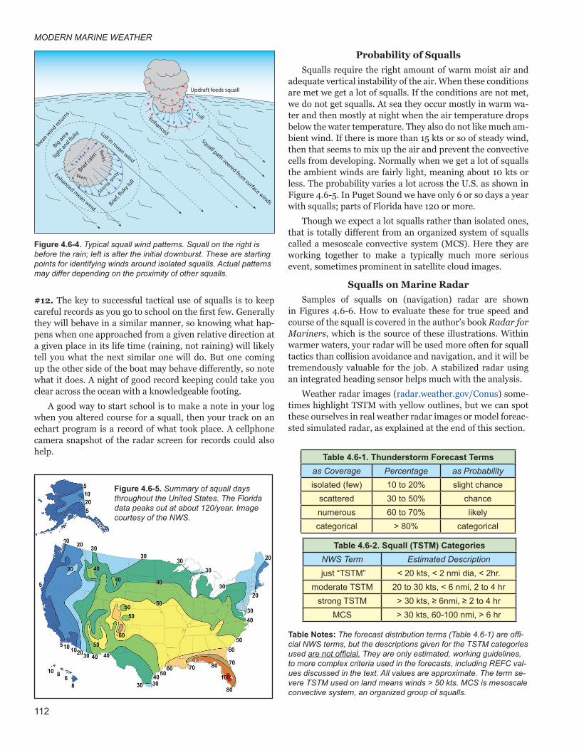
Figure 4.6-4. Typical squall wind patterns. Squall on the right is before the rain; left is after the initial downburst. These are starting points for identifying winds around isolated squalls. Actual patterns may differ depending on the proximity of other squalls.

#12. The key to successful tactical use of squalls is to keep careful records as you go to school on the first few. Generally they will behave in a similar manner, so knowing what hap-pens when one approached from a given relative direction at a given place in its life time (raining, not raining) will likely tell you what the next similar one will do. But one coming up the other side of the boat may behave differently, so note what it does. A night of good record keeping could take you clear across the ocean with a knowledgeable footing.

A good way to start school is to make a note in your log when you altered course for a squall, then your track on an echart program is a record of what took place. A cellphone camera snapshot of the radar screen for records could also help.

Probability of SquallsSqualls require the right amount of warm moist air and

adequate vertical instability of the air. When these conditions are met we get a lot of squalls. If the conditions are not met, we do not get squalls. At sea they occur mostly in warm wa-ter and then mostly at night when the air temperature drops below the water temperature. They also do not like much am-bient wind. If there is more than 15 kts or so of steady wind, then that seems to mix up the air and prevent the convective cells from developing. Normally when we get a lot of squalls the ambient winds are fairly light, meaning about 10 kts or less. The probability varies a lot across the U.S. as shown in Figure 4.6-5. In Puget Sound we have only 6 or so days a year with squalls; parts of Florida have 120 or more.

Though we expect a lot squalls rather than isolated ones, that is totally different from an organized system of squalls called a mesoscale convective system (MCS). Here they are working together to make a typically much more serious event, sometimes prominent in satellite cloud images.

Squalls on Marine RadarSamples of squalls on (navigation) radar are shown

in Figures 4.6-6. How to evaluate these for true speed and course of the squall is covered in the author’s book Radar for Mariners, which is the source of these illustrations. Within warmer waters, your radar will be used more often for squall tactics than collision avoidance and navigation, and it will be tremendously valuable for the job. A stabilized radar using an integrated heading sensor helps much with the analysis.

Weather radar images (radar.weather.gov/Conus) some-times highlight TSTM with yellow outlines, but we can spot these ourselves in real weather radar images or model foreac-sted simulated radar, as explained at the end of this section.

Enhanced

Lull

Squall path veered from surface winds

Updraft feeds squall

Brief, �

uky lull

Enhanced mean wind

Lull in mean wind

Big area

light a

nd �ukyBrie

f calm

Strong, g

ustyVeers

Backs

Mean wind re

turn

s

Figure 4.6-5. Summary of squall days throughout the United States. The Florida data peaks out at about 120/year. Image courtesy of the NWS.

Table 4.6-1. Thunderstorm Forecast Termsas Coverage Percentage as Probabilityisolated (few) 10 to 20% slight chance

scattered 30 to 50% chancenumerous 60 to 70% likelycategorical > 80% categorical

Table 4.6-2. Squall (TSTM) CategoriesNWS Term Estimated Description

just “TSTM” < 20 kts, < 2 nmi dia, < 2hr.moderate TSTM 20 to 30 kts, < 6 nmi, 2 to 4 hr

strong TSTM > 30 kts, ≥ 6nmi, ≥ 2 to 4 hr MCS > 30 kts, 60-100 nmi, > 6 hr

Table Notes: The forecast distribution terms (Table 4.6-1) are offi-cial NWS terms, but the descriptions given for the TSTM categories used are not official. They are only estimated, working guidelines, to more complex criteria used in the forecasts, including REFC val-ues discussed in the text. All values are approximate. The term se-vere TSTM used on land means winds > 50 kts. MCS is mesoscale convective system, an organized group of squalls.

MODERN MARINE WEATHER

114

You will often see long lines of individual squalls at sea, with one squall after another formed in a distinct line, but these do not make up a squall line. A squall line is not a line of squalls. A line of squalls has some level of gap apparent in the radar image of the row of squalls. But real squall lines are different systems. They will draw a bright white smear across your radar screen as far as the radar can see. These are not like normal squalls, and they do not move like normal squalls.

I confronted a real squall line once not far from the Baha-mas. In that case we could clearly see one end of the system visually, and what appeared to be the other end, but it wasn’t. The true extent of it was awesome on radar. We put the pedal to the metal and actually managed to scoot around the end of it, pushing a big bow wave and burning up a lot of fuel. We later learned of the great damage it did to several vessels that did not escape it.

A fast moving cold front, snow-plowing air in front of it as it proceeds, is often the source of extra lift needed to form a squall line, but there are also other rarer conditions of insta-bility that can create these. The mechanisms are complex and diverse. Squall lines formed by fast cold fronts are typically some 100 miles ahead of the front and parallel to it.

Squall lines can sometimes be seen in satellite images or ASCAT measurements in which case they could be forecasted, but more often than not these powerful systems are not fore-casted at sea. On land they are usually spotted and tracked in weather radar images and wind warnings announced in advance.

Squalls in Model ForecastsA new development in marine weather is the availability

of simulated radar forecasts, which is just what it sounds like—digital forecasts of what the weather radar will look like in the future; in a sense, the ideal way to forecast squalls or convective activity of any kind. This parameter, composite re-flectivity (REFC), is available in any of the WRF based mod-els, such as HRRR, NAM, and NBM discussed in Chapter 7. These are hi-res forecasts, some updated hourly, extending

out a day or two. We can’t really hope for longer; squalls are dynamic, transient systems.

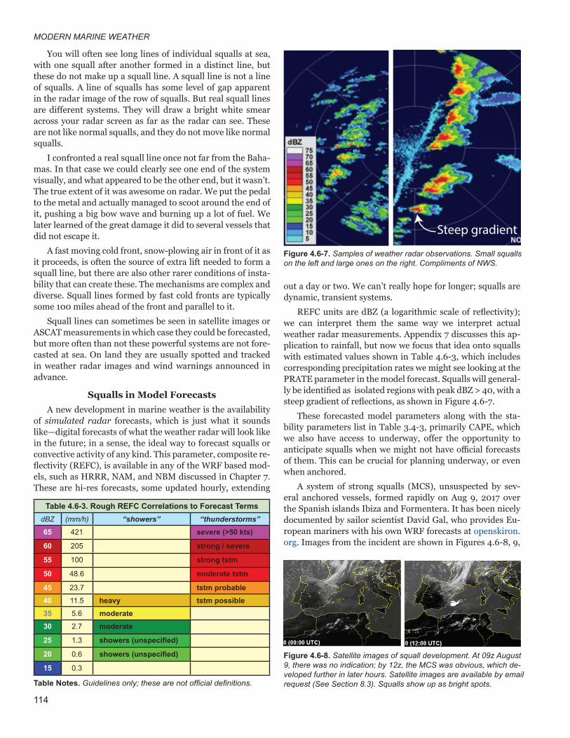
REFC units are dBZ (a logarithmic scale of reflectivity); we can interpret them the same way we interpret actual weather radar measurements. Appendix 7 discusses this ap-plication to rainfall, but now we focus that idea onto squalls with estimated values shown in Table 4.6-3, which includes corresponding precipitation rates we might see looking at the PRATE parameter in the model forecast. Squalls will general-ly be identified as isolated regions with peak dBZ > 40, with a steep gradient of reflections, as shown in Figure 4.6-7.

These forecasted model parameters along with the sta-bility parameters list in Table 3.4-3, primarily CAPE, which we also have access to underway, offer the opportunity to anticipate squalls when we might not have official forecasts of them. This can be crucial for planning underway, or even when anchored.

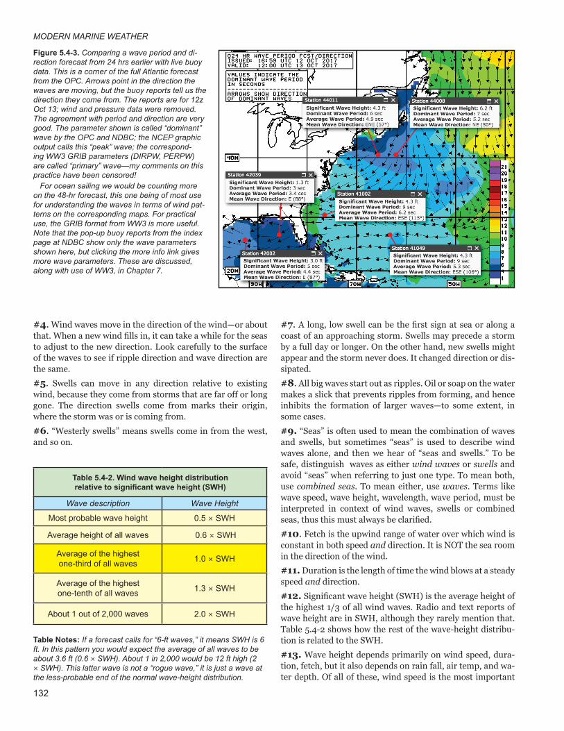
A system of strong squalls (MCS), unsuspected by sev-eral anchored vessels, formed rapidly on Aug 9, 2017 over the Spanish islands Ibiza and Formentera. It has been nicely documented by sailor scientist David Gal, who provides Eu-ropean mariners with his own WRF forecasts at openskiron.org. Images from the incident are shown in Figures 4.6-8, 9,

Table 4.6-3. Rough REFC Correlations to Forecast TermsdBZ (mm/h) “showers” “thunderstorms”65 421 severe (>50 kts)

60 205 strong / severe

55 100 strong tstm

50 48.6 moderate tstm

45 23.7 tstm probable40 11.5 heavy tstm possible35 5.6 moderate30 2.7 moderate

25 1.3 showers (unspecified)

20 0.6 showers (unspecified)

15 0.3

Steep gradientSteep gradient

Figure 4.6-7. Samples of weather radar observations. Small squalls on the left and large ones on the right. Compliments of NWS.

Table Notes. Guidelines only; these are not official definitions.

Figure 4.6-8. Satellite images of squall development. At 09z August 9, there was no indication; by 12z, the MCS was obvious, which de-veloped further in later hours. Satellite images are available by email request (See Section 8.3). Squalls show up as bright spots.

MODERN MARINE WEATHER

132

Table 5.4-2. Wind wave height distributionrelative to significant wave height (SWH)

Wave description Wave Height

Most probable wave height 0.5 × SWH

Average height of all waves 0.6 × SWH

Average of the highest one-third of all waves 1.0 × SWH

Average of the highest one-tenth of all waves 1.3 × SWH

About 1 out of 2,000 waves 2.0 × SWH

Table Notes: If a forecast calls for “6-ft waves,” it means SWH is 6 ft. In this pattern you would expect the average of all waves to be about 3.6 ft (0.6 × SWH). About 1 in 2,000 would be 12 ft high (2 × SWH). This latter wave is not a “rogue wave,” it is just a wave at the less-probable end of the normal wave-height distribution.

#4. Wind waves move in the direction of the wind—or about that. When a new wind fills in, it can take a while for the seas to adjust to the new direction. Look carefully to the surface of the waves to see if ripple direction and wave direction are the same.#5. Swells can move in any direction relative to existing wind, because they come from storms that are far off or long gone. The direction swells come from marks their origin, where the storm was or is coming from.#6. “Westerly swells” means swells come in from the west, and so on.

#7. A long, low swell can be the first sign at sea or along a coast of an approaching storm. Swells may precede a storm by a full day or longer. On the other hand, new swells might appear and the storm never does. It changed direction or dis-sipated.#8. All big waves start out as ripples. Oil or soap on the water makes a slick that prevents ripples from forming, and hence inhibits the formation of larger waves—to some extent, in some cases.#9. “Seas” is often used to mean the combination of waves and swells, but sometimes “seas” is used to describe wind waves alone, and then we hear of “seas and swells.” To be safe, distinguish waves as either wind waves or swells and avoid “seas” when referring to just one type. To mean both, use combined seas. To mean either, use waves. Terms like wave speed, wave height, wavelength, wave period, must be interpreted in context of wind waves, swells or combined seas, thus this must always be clarified.#10. Fetch is the upwind range of water over which wind is constant in both speed and direction. It is NOT the sea room in the direction of the wind.#11. Duration is the length of time the wind blows at a steady speed and direction.#12. Significant wave height (SWH) is the average height of the highest 1/3 of all wind waves. Radio and text reports of wave height are in SWH, although they rarely mention that. Table 5.4-2 shows how the rest of the wave-height distribu-tion is related to the SWH.#13. Wave height depends primarily on wind speed, dura-tion, fetch, but it also depends on rain fall, air temp, and wa-ter depth. Of all of these, wind speed is the most important

Figure 5.4-3. Comparing a wave period and di-rection forecast from 24 hrs earlier with live buoy data. This is a corner of the full Atlantic forecast from the OPC. Arrows point in the direction the waves are moving, but the buoy reports tell us the direction they come from. The reports are for 12z Oct 13; wind and pressure data were removed. The agreement with period and direction are very good. The parameter shown is called “dominant” wave by the OPC and NDBC; the NCEP graphic output calls this “peak” wave; the correspond-ing WW3 GRIB parameters (DIRPW, PERPW) are called “primary” wave—my comments on this practice have been censored!

For ocean sailing we would be counting more on the 48-hr forecast, this one being of most use for understanding the waves in terms of wind pat-terns on the corresponding maps. For practical use, the GRIB format from WW3 is more useful. Note that the pop-up buoy reports from the index page at NDBC show only the wave parameters shown here, but clicking the more info link gives more wave parameters. These are discussed, along with use of WW3, in Chapter 7.

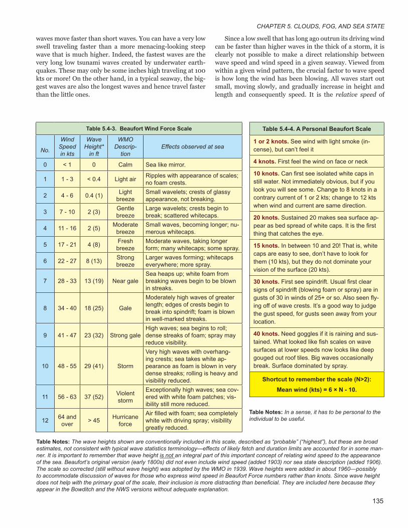
CHAPTER 5. CLOUDS, FOG, AND SEA STATE

135

Table 5.4-3. Beaufort Wind Force Scale

No.

Wind Speed in kts

Wave Height*

in ft

WMO Descrip-

tionEffects observed at sea

0 < 1 0 Calm Sea like mirror.

1 1 - 3 < 0.4 Light air Ripples with appearance of scales; no foam crests.

2 4 - 6 0.4 (1) Light breeze

Small wavelets; crests of glassy appearance, not breaking.

3 7 - 10 2 (3) Gentle breeze

Large wavelets; crests begin to break; scattered whitecaps.

4 11 - 16 2 (5) Moderate breeze

Small waves, becoming longer; nu-merous whitecaps.

5 17 - 21 4 (8) Fresh breeze

Moderate waves, taking longer form; many whitecaps; some spray.

6 22 - 27 8 (13) Strong breeze

Larger waves forming; whitecaps everywhere; more spray.

7 28 - 33 13 (19) Near galeSea heaps up; white foam from breaking waves begin to be blown in streaks.

8 34 - 40 18 (25) Gale

Moderately high waves of greater length; edges of crests begin to break into spindrift; foam is blown in well-marked streaks.

9 41 - 47 23 (32) Strong galeHigh waves; sea begins to roll; dense streaks of foam; spray may reduce visibility.

10 48 - 55 29 (41) Storm

Very high waves with overhang-ing crests; sea takes white ap-pearance as foam is blown in very dense streaks; rolling is heavy and visibility reduced.

11 56 - 63 37 (52) Violent storm

Exceptionally high waves; sea cov-ered with white foam patches; vis-ibility still more reduced.

12 64 and over > 45 Hurricane

force

Air filled with foam; sea completely white with driving spray; visibility greatly reduced.

Table Notes: The wave heights shown are conventionally included in this scale, described as “probable” (“highest”), but these are broad estimates, not consistent with typical wave statistics terminology—effects of likely fetch and duration limits are accounted for in some man-ner. It is important to remember that wave height is not an integral part of this important concept of relating wind speed to the appearance of the sea. Beaufort’s original version (early 1800s) did not even include wind speed (added 1903) nor sea state description (added 1906). The scale so corrected (still without wave height) was adopted by the WMO in 1939. Wave heights were added in about 1960—possibly to accommodate discussion of waves for those who express wind speed in Beaufort Force numbers rather than knots. Since wave height does not help with the primary goal of the scale, their inclusion is more distracting than beneficial. They are included here because they appear in the Bowditch and the NWS versions without adequate explanation.

waves move faster than short waves. You can have a very low swell traveling faster than a more menacing-looking steep wave that is much higher. Indeed, the fastest waves are the very long low tsunami waves created by underwater earth-quakes. These may only be some inches high traveling at 100 kts or more! On the other hand, in a typical seaway, the big-gest waves are also the longest waves and hence travel faster than the little ones.

Since a low swell that has long ago outrun its driving wind can be faster than higher waves in the thick of a storm, it is clearly not possible to make a direct relationship between wave speed and wind speed in a given seaway. Viewed from within a given wind pattern, the crucial factor to wave speed is how long the wind has been blowing. All waves start out small, moving slowly, and gradually increase in height and length and consequently speed. It is the relative speed of

Table 5.4-4. A Personal Beaufort Scale

1 or 2 knots. See wind with light smoke (in-cense), but can’t feel it

4 knots. First feel the wind on face or neck

10 knots. Can first see isolated white caps in still water. Not immediately obvious, but if you look you will see some. Change to 8 knots in a contrary current of 1 or 2 kts; change to 12 kts when wind and current are same direction.

20 knots. Sustained 20 makes sea surface ap-pear as bed spread of white caps. It is the first thing that catches the eye.

15 knots. In between 10 and 20! That is, white caps are easy to see, don’t have to look for them (10 kts), but they do not dominate your vision of the surface (20 kts).

30 knots. First see spindrift. Usual first clear signs of spindrift (blowing foam or spray) are in gusts of 30 in winds of 25+ or so. Also seen fly-ing off of wave crests. It’s a good way to judge the gust speed, for gusts seen away from your location.

40 knots. Need goggles if it is raining and sus-tained. What looked like fish scales on wave surfaces at lower speeds now looks like deep gouged out roof tiles. Big waves occasionally break. Surface dominated by spray.

Shortcut to remember the scale (N>2):Mean wind (kts) = 6 × N - 10.

Table Notes: In a sense, it has to be personal to the individual to be useful.

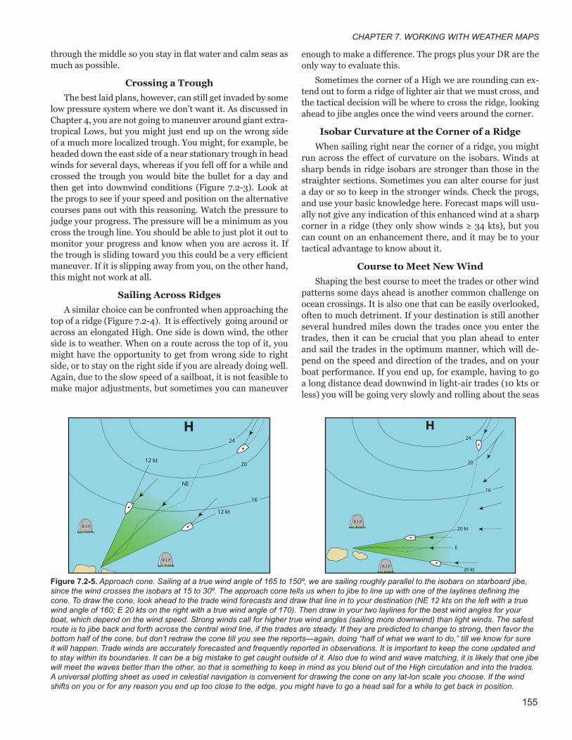
CHAPTER 7. WORKING WITH WEATHER MAPS

155

through the middle so you stay in flat water and calm seas as much as possible.

Crossing a TroughThe best laid plans, however, can still get invaded by some

low pressure system where we don’t want it. As discussed in Chapter 4, you are not going to maneuver around giant extra-tropical Lows, but you might just end up on the wrong side of a much more localized trough. You might, for example, be headed down the east side of a near stationary trough in head winds for several days, whereas if you fell off for a while and crossed the trough you would bite the bullet for a day and then get into downwind conditions (Figure 7.2-3). Look at the progs to see if your speed and position on the alternative courses pans out with this reasoning. Watch the pressure to judge your progress. The pressure will be a minimum as you cross the trough line. You should be able to just plot it out to monitor your progress and know when you are across it. If the trough is sliding toward you this could be a very efficient maneuver. If it is slipping away from you, on the other hand, this might not work at all.

Sailing Across Ridges A similar choice can be confronted when approaching the

top of a ridge (Figure 7.2-4). It is effectively going around or across an elongated High. One side is down wind, the other side is to weather. When on a route across the top of it, you might have the opportunity to get from wrong side to right side, or to stay on the right side if you are already doing well. Again, due to the slow speed of a sailboat, it is not feasible to make major adjustments, but sometimes you can maneuver

enough to make a difference. The progs plus your DR are the only way to evaluate this.

Sometimes the corner of a High we are rounding can ex-tend out to form a ridge of lighter air that we must cross, and the tactical decision will be where to cross the ridge, looking ahead to jibe angles once the wind veers around the corner.

Isobar Curvature at the Corner of a RidgeWhen sailing right near the corner of a ridge, you might

run across the effect of curvature on the isobars. Winds at sharp bends in ridge isobars are stronger than those in the straighter sections. Sometimes you can alter course for just a day or so to keep in the stronger winds. Check the progs, and use your basic knowledge here. Forecast maps will usu-ally not give any indication of this enhanced wind at a sharp corner in a ridge (they only show winds ≥ 34 kts), but you can count on an enhancement there, and it may be to your tactical advantage to know about it.

Course to Meet New WindShaping the best course to meet the trades or other wind

patterns some days ahead is another common challenge on ocean crossings. It is also one that can be easily overlooked, often to much detriment. If your destination is still another several hundred miles down the trades once you enter the trades, then it can be crucial that you plan ahead to enter and sail the trades in the optimum manner, which will de-pend on the speed and direction of the trades, and on your boat performance. If you end up, for example, having to go a long distance dead downwind in light-air trades (10 kts or less) you will be going very slowly and rolling about the seas

Figure 7.2-5. Approach cone. Sailing at a true wind angle of 165 to 150º, we are sailing roughly parallel to the isobars on starboard jibe, since the wind crosses the isobars at 15 to 30º. The approach cone tells us when to jibe to line up with one of the laylines defining the cone. To draw the cone, look ahead to the trade wind forecasts and draw that line in to your destination (NE 12 kts on the left with a true wind angle of 160; E 20 kts on the right with a true wind angle of 170). Then draw in your two laylines for the best wind angles for your boat, which depend on the wind speed. Strong winds call for higher true wind angles (sailing more downwind) than light winds. The safest route is to jibe back and forth across the central wind line, if the trades are steady. If they are predicted to change to strong, then favor the bottom half of the cone, but don’t redraw the cone till you see the reports—again, doing “half of what we want to do,” till we know for sure it will happen. Trade winds are accurately forecasted and frequently reported in observations. It is important to keep the cone updated and to stay within its boundaries. It can be a big mistake to get caught outside of it. Also due to wind and wave matching, it is likely that one jibe will meet the waves better than the other, so that is something to keep in mind as you blend out of the High circulation and into the trades. A universal plotting sheet as used in celestial navigation is convenient for drawing the cone on any lat-lon scale you choose. If the wind shifts on you or for any reason you end up too close to the edge, you might have to go a head sail for a while to get back in position.

24

20

16

12 kt

12 kt

NE

H

R.I.P.

R.I.P.

24

20

16

20 kt

E

H

20 kt

R.I.P.

R.I.P.

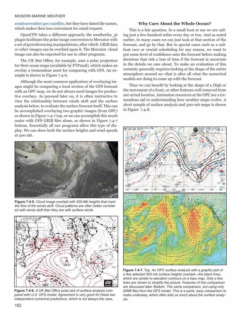
MODERN MARINE WEATHER

162

Why Care About the Whole Ocean?This is a fair question. In a small boat at sea we are sail-

ing just a few hundred miles every day or two. And as noted earlier, in many cases we can just look at that section of the forecast, and go by that. But in special cases such as a sail-boat race or crucial scheduling for any reason, we want to put some level of confidence onto the forecast before making decisions that risk a loss of time if the forecast is uncertain in the details we care about. To make an evaluation of this certainty generally requires looking at the shape of the entire atmosphere around us—that is after all what the numerical models are doing to come up with the forecast.

Thus we can benefit by looking at the shape of a High or the movement of a front, or other features well removed from our actual location. Animation resources at the OPC are a tre-mendous aid to understanding how weather maps evolve. A short sample of surface analysis and 500-mb maps is shown in Figure 7.4-8.

Figure 7.4-5. Cloud image overlaid with 500-Mb heights that mark the flow of the winds aloft. Cloud patterns are often better correlat-ed with winds aloft than they are with surface winds.

aviationweather.gov/satellite, but they have dated file names, which makes then less convenient for email request.

OpenCPN takes a different approach; the weatherfax_pi plugin facilitates the polar image conversion to Mercator with a set of georeferencing manipulations, after which GRIB data or other images can be overlaid upon it. The Mercator cloud image can also be exported for use in other programs.

The UK Met Office, for example, uses a polar projection for their ocean maps (available by FTPmail), which makes an overlay a tremendous asset for comparing with GFS. An ex-ample is shown in Figure 7.4-6.

Although the most common application of overlaying im-ages might be comparing a local section of the GFS forecast with an OPC map, we do not always need images for produc-tive overlays. As pursued later on, it is often instructive to view the relationship between winds aloft and the surface analysis below, to evaluate the surface forecast itself. This can be accomplished overlaying two graphic images (from OPC) as shown in Figure 7.4-7 top, or we can accomplish this much easier with GFS GRIB files alone, as shown in Figure 7.4-7 bottom. Essentially all nav programs allow this type of dis-play. We can show both the surface heights and wind speeds at 500 mb.

Figure 7.4-7. Top. An OPC surface analysis with a graphic plot of a few selected 500 mb surface heights overlaid—the black lines, which are similar to elevation contours on a topo map. Only a few lines are shown to simplify the picture. Features of this comparison are discussed later. Bottom. The same comparison, but using only GRIB files from the GFS model. This is a quick, easy comparison to make underway, which often tells us much about the surface analy-sis.

Figure 7.4-6. A UK Met Office polar plot of surface analysis com-pared with U.S. GFS model. Agreement is very good for these two independent numerical predictions, which is not always the case.

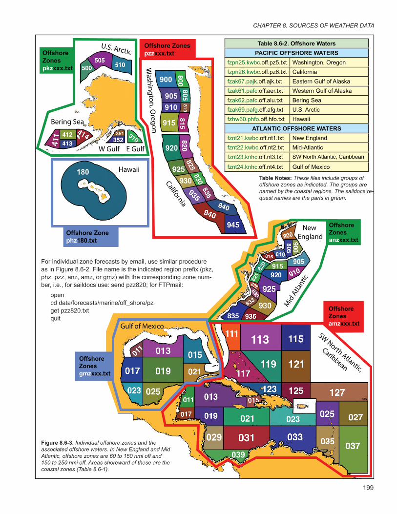
CHAPTER 8. SOURCES OF WEATHER DATA

199

New England

Mid

Atla

ntic

Offshore Zonesanzxxx.txt

Offshore Zonesamzxxx.txt

SW North Atlantic,

CaribbeanOffshore Zonesgmzxxx.txt

Gulf of Mexico

Offshore Zonespkzxxx.txt

Bering Sea

W Gulf E Gulf

U.S. Arctic

Offshore Zonephz180.txt

Washington, O

regon

California

Hawaii

029

039

Offshore Zonespzzxxx.txt

180

900

905910

915

920

Figure 8.6-3. Individual offshore zones and the associated offshore waters. In New England and Mid Atlantic, offshore zones are 60 to 150 nmi off and 150 to 250 nmi off. Areas shoreward of these are the coastal zones (Table 8.6-1).

For individual zone forecasts by email, use similar procedure as in Figure 8.6-2. File name is the indicated region prefix (pkz, phz, pzz, anz, amz, or gmz) with the corresponding zone num-ber, i.e., for saildocs use: send pzz820; for FTPmail:

open cd data/forecasts/marine/off_shore/pz get pzz820.txt quit

New England

Mid

Atla

ntic

Offshore Zonesanzxxx.txt

Offshore Zonesamzxxx.txt

SW North Atlantic,

CaribbeanOffshore Zonesgmzxxx.txt

Gulf of Mexico

Offshore Zonespkzxxx.txt

Bering Sea

W Gulf E Gulf

U.S. Arctic

Offshore Zonephz180.txtW

ashington, Oregon

California

Hawaii

029

039

Offshore Zonespzzxxx.txt

180

900

905910

915

920

Table 8.6-2. Offshore WatersPACIFIC OFFSHORE WATERS

fzpn25.kwbc.off.pz5.txt Washington, Oregonfzpn26.kwbc.off.pz6.txt Californiafzak67.pajk.off.ajk.txt Eastern Gulf of Alaskafzak61.pafc.off.aer.txt Western Gulf of Alaskafzak62.pafc.off.alu.txt Bering Seafzak69.pafg.off.afg.txt U.S. Arcticfzhw60.phfo.off.hfo.txt Hawaii

ATLANTIC OFFSHORE WATERSfznt21.kwbc.off.nt1.txt New Englandfznt22.kwbc.off.nt2.txt Mid-Atlanticfznt23.knhc.off.nt3.txt SW North Atlantic, Caribbean

fznt24.knhc.off.nt4.txt Gulf of Mexico

Table Notes: These files include groups of offshore zones as indicated. The groups are named by the coastal regions. The saildocs re-quest names are the parts in green.

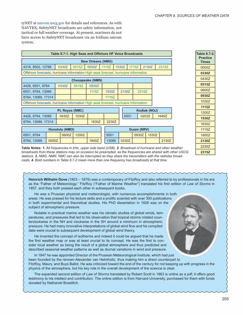
CHAPTER 8. SOURCES OF WEATHER DATA

205

Table Notes: 1. All frequencies in kHz, upper side band (USB). 2. Broadcast of hurricane and other weather broadcasts from these stations may on occasion be preempted, as the frequencies are shared with other USCG stations. 3. NMG, NMN, NMC can also be interrupted as they share the transmitters with the radiofax broad-casts. 4. Bold numbers in Table 8.7-2 mean more than one frequency has broadcasts at that time.

Table 8.7-1. High Seas and Offshore HF Voice Broadcasts

New Orleans (NMG) 4316, 8502, 12788 0330Z 0515Z 0930Z 1115Z 1530Z 1715Z 2130Z 2315Z

Offshore forecasts, hurricane information High seas forecast, hurricane information

Chesapeake (NMN) 4426, 6501, 8764 0330Z 0515Z 0930Z

6501, 8764, 13089 1115Z 1530Z 2130Z 2315Z

8764, 13089, 17314 1715Z

Offshore forecasts, hurricane information High seas forecast, hurricane information

Pt. Reyes (NMC) Kodiak (NOJ)4426, 8764, 13089 0430Z 1030Z 6501 0203Z 1645Z

8764, 13089, 17314 1630Z 2230Z

Honolulu (NMO) Guam (NRV)6501, 8764 0600Z 1200Z 6501 0930Z 1530Z

8764, 13089 0005Z 1800Z 13089 0330Z 2130Z

Heinrich Wilhelm Dove (1803 – 1879) was a contemporary of FitzRoy and also referred to by professionals in his era as the “Father of Meteorology.” FitzRoy (“Father of Marine Weather”) translated his first edition of Law of Storms in 1857, and they both praised each other in subsequent books.

He was a Prussian physicist and meteorologist, with numerous accomplishments in both areas. He was praised for his lecture skills and a prolific scientist with over 300 publications in both experimental and theoretical studies. His PhD dissertation in 1826 was on the subject of atmospheric pressure.

Notable in practical marine weather was his climatic studies of global winds, tem-peratures, and pressures that led to his observation that tropical storms rotated coun-terclockwise in the NH and clockwise in the SH around a minimum in atmospheric pressure. He had many innovative interpretations of global wind flow and his compiled data were crucial to subsequent development of global wind theory.

He invented the concept of isotherms and indeed it could be argued that he made the first weather map or was at least crucial to its concept. He was the first to con-sider local weather as being the result of a global atmosphere and thus predicted and described seasonal weather patterns as well as diurnal variations in wind and pressure.

In 1847 he was appointed Director of the Prussian Meteorological Institute, which had just been founded by the renown Alexander van Helmholtz, thus making him a direct counterpart to FitzRoy, Maury, and Buys Ballot. He was criticized toward the end of the century for not keeping up with progress in the physics of the atmosphere, but his key role in the overall development of the science is clear.

The expanded second edition of Law of Storms translated by Robert Scott in 1863 is online as a pdf; it offers good testimony to his intellect and contribution. The online edition is from Harvard University, purchased for them with funds donated by Nathaniel Bowditch.

Table 8.7-2. Practice Times0005Z

0330Z0430Z

0515Z0600Z

0930Z1030Z

1115Z1200Z

1530Z1630Z

1715Z

1800Z

2130Z2230Z

2315Z

tyNET at navcen.uscg.gov for details and references. As with NAVTEX, SafetyNET broadcasts are safety information, not tactical or full weather coverage. At present, mariners do not have access to SafetyNET broadcasts via an Iridium satcom system.

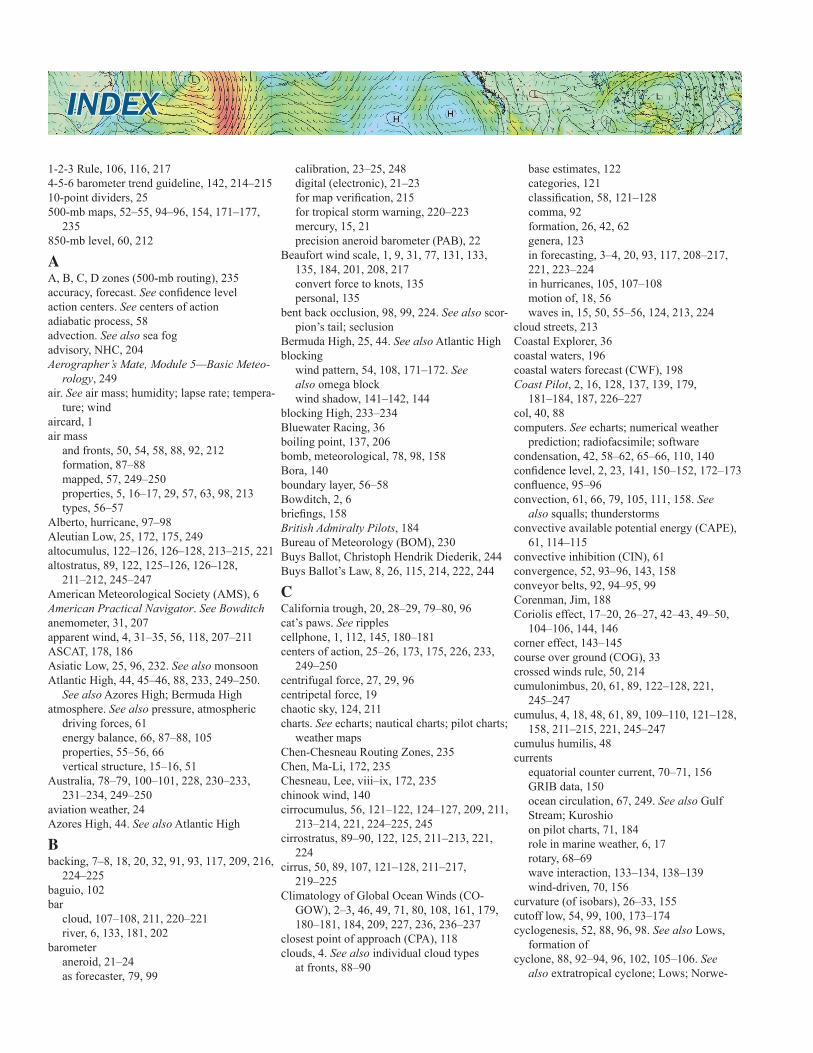
1-2-3 Rule, 106, 116, 2174-5-6 barometer trend guideline, 142, 214–21510-point dividers, 25500-mb maps, 52–55, 94–96, 154, 171–177,

235850-mb level, 60, 212

AA, B, C, D zones (500-mb routing), 235accuracy, forecast. See confidence levelaction centers. See centers of actionadiabatic process, 58advection. See also sea fogadvisory, NHC, 204Aerographer’s Mate, Module 5—Basic Meteo-

rology, 249air. See air mass; humidity; lapse rate; tempera-

ture; windaircard, 1air mass

and fronts, 50, 54, 58, 88, 92, 212formation, 87–88mapped, 57, 249–250properties, 5, 16–17, 29, 57, 63, 98, 213types, 56–57

Alberto, hurricane, 97–98Aleutian Low, 25, 172, 175, 249altocumulus, 122–126, 126–128, 213–215, 221altostratus, 89, 122, 125–126, 126–128,

211–212, 245–247American Meteorological Society (AMS), 6American Practical Navigator. See Bowditchanemometer, 31, 207apparent wind, 4, 31–35, 56, 118, 207–211ASCAT, 178, 186Asiatic Low, 25, 96, 232. See also monsoonAtlantic High, 44, 45–46, 88, 233, 249–250.

See also Azores High; Bermuda Highatmosphere. See also pressure, atmospheric

driving forces, 61energy balance, 66, 87–88, 105properties, 55–56, 66vertical structure, 15–16, 51

Australia, 78–79, 100–101, 228, 230–233, 231–234, 249–250

aviation weather, 24Azores High, 44. See also Atlantic High

Bbacking, 7–8, 18, 20, 32, 91, 93, 117, 209, 216,

224–225baguio, 102bar

cloud, 107–108, 211, 220–221river, 6, 133, 181, 202

barometeraneroid, 21–24as forecaster, 79, 99

calibration, 23–25, 248digital (electronic), 21–23for map verification, 215for tropical storm warning, 220–223mercury, 15, 21precision aneroid barometer (PAB), 22

Beaufort wind scale, 1, 9, 31, 77, 131, 133, 135, 184, 201, 208, 217convert force to knots, 135personal, 135

bent back occlusion, 98, 99, 224. See also scor-pion’s tail; seclusion

Bermuda High, 25, 44. See also Atlantic Highblocking

wind pattern, 54, 108, 171–172. See also omega blockwind shadow, 141–142, 144

blocking High, 233–234Bluewater Racing, 36boiling point, 137, 206bomb, meteorological, 78, 98, 158Bora, 140boundary layer, 56–58Bowditch, 2, 6briefings, 158British Admiralty Pilots, 184Bureau of Meteorology (BOM), 230Buys Ballot, Christoph Hendrik Diederik, 244Buys Ballot’s Law, 8, 26, 115, 214, 222, 244

CCalifornia trough, 20, 28–29, 79–80, 96cat’s paws. See ripplescellphone, 1, 112, 145, 180–181centers of action, 25–26, 173, 175, 226, 233,

249–250centrifugal force, 27, 29, 96centripetal force, 19chaotic sky, 124, 211charts. See echarts; nautical charts; pilot charts;

weather mapsChen-Chesneau Routing Zones, 235Chen, Ma-Li, 172, 235Chesneau, Lee, viii–ix, 172, 235chinook wind, 140cirrocumulus, 56, 121–122, 124–127, 209, 211,

213–214, 221, 224–225, 245cirrostratus, 89–90, 122, 125, 211–213, 221,

224cirrus, 50, 89, 107, 121–128, 211–217,

219–225Climatology of Global Ocean Winds (CO-

GOW), 2–3, 46, 49, 71, 80, 108, 161, 179, 180–181, 184, 209, 227, 236, 236–237

closest point of approach (CPA), 118clouds, 4. See also individual cloud types

at fronts, 88–90

base estimates, 122categories, 121classification, 58, 121–128comma, 92formation, 26, 42, 62genera, 123in forecasting, 3–4, 20, 93, 117, 208–217, 221, 223–224in hurricanes, 105, 107–108motion of, 18, 56waves in, 15, 50, 55–56, 124, 213, 224

cloud streets, 213Coastal Explorer, 36coastal waters, 196coastal waters forecast (CWF), 198Coast Pilot, 2, 16, 128, 137, 139, 179,

181–184, 187, 226–227col, 40, 88computers. See echarts; numerical weather

prediction; radiofacsimile; softwarecondensation, 42, 58–62, 65–66, 110, 140confidence level, 2, 23, 141, 150–152, 172–173confluence, 95–96convection, 61, 66, 79, 105, 111, 158. See

also squalls; thunderstormsconvective available potential energy (CAPE),

61, 114–115convective inhibition (CIN), 61convergence, 52, 93–96, 143, 158conveyor belts, 92, 94–95, 99Corenman, Jim, 188Coriolis effect, 17–20, 26–27, 42–43, 49–50,

104–106, 144, 146corner effect, 143–145course over ground (COG), 33crossed winds rule, 50, 214cumulonimbus, 20, 61, 89, 122–128, 221,

245–247cumulus, 4, 18, 48, 61, 89, 109–110, 121–128,

158, 211–215, 221, 245–247cumulus humilis, 48currents

equatorial counter current, 70–71, 156GRIB data, 150ocean circulation, 67, 249. See also Gulf Stream; Kuroshioon pilot charts, 71, 184role in marine weather, 6, 17rotary, 68–69wave interaction, 133–134, 138–139wind-driven, 70, 156

curvature (of isobars), 26–33, 155cutoff low, 54, 99, 100, 173–174cyclogenesis, 52, 88, 96, 98. See also Lows,

formation ofcyclone, 88, 92–94, 96, 102, 105–106. See

also extratropical cyclone; Lows; Norwe-

INDEX

INDEX

261

About the Author

David Burch is a Fellow of the Royal Institute of Navigation in London as well as a Fellow of the Institute of Navigation in Washington, DC, from which he received the Superior Achievement Award for outstanding performance as a practicing navigator. He has logged more than 70,000 miles at sea, including twelve transoceanic yacht races, with several first place victories and a passage record for boats under 36 feet that lasted 16 years. He also navigated the only American entry in the storm-ridden 1993 Sydney to Hobart Race.

On the academic side, he is a former Fulbright Scholar with a PhD in physics. As Founding Director of Starpath School of Navigation in Seattle he has designed courses and taken part in the teaching of marine weather and navigation for more than 30 years. He continues to work on the development of online training materials, which are presented at starpath.com. His articles on special topics in navigation and weather appear at starpath.com/articles.

Other books by the author

Weather WorkbookThe Barometer HandbookMariner’s Pressure AtlasIntroduction to Electronic Chart Navigation Celestial NavigationInland and Coastal NavigationRadar for MarinersFundamentals of Kayak NavigationSailor’s LogbookEmergency NavigationThe Star Finder BookHawaii By SextantHow to Use Plastic Sextants

Starpath Publications, Seattle WAwww.starpathpublications.com

MO

DERN

MA

RINE W

EATH

ERTH

IRD ED

ITION

BU

RCH

“A thoughtfully and masterfully crafted work. It will be my prime recommendation of a book focusing specifi cally on the application of weather information and knowledge for maritime interests, whatever the size and purpose of the vessel. David thoroughly explores the essentials of meteorology, and does so in a fascinating manner. Reading and absorbing these principles and applications will lead to safer, faster and more effi cient passages.”—Jeff Renner, Meteorologist, King 5 TV, Seattle,WA.

“I have chosen this book as the defi nitive text for the wardroom of my U.S. Navy Destroyer. Superior explanations that are as useful for the professional naval offi cer as they are for the coastal pleasure cruiser or blue water sailor. Consistent with all of David Burch’s texts: Easy to read, fascinating, and the absolute best resource.” —CDR Tate Westbrook, CO USS Spruance (DDG111)

“First class reference book on the subject of marine weather and the information it contains will help every sailor, every day!” — Peter Isler, two-time America’s Cup winning navigator

“An essential reference for the coastal and offshore sailor. It goes far beyond the traditional marine weather books. …an excellent job of laying proper foundations for understanding marine weather, and bringing clarity to a complex topic.” —Jim Corenman, developer of Saildocs and SailMail

“The defi nitive text for those wanting to learn more about marine meteorology. …David Burch should be applauded for this beautiful piece of work.” —Kenn Batt, Australian Bureau of Meteorology, Sydney to Hobart Race weather briefer

“An instant classic. If you own one book about weather this is it. If you want to make your own intelligent forecast and pick-up local knowledge like a local, you will fi nd all the information in this most excellent book.” —Philippe Kahn, CEO, FullPower Technologies, Doublehanded Transpacifi c record holder

“A new and truly extraordinary treatise on an age old subject. Principles and scientifi c conclusions expertly revealed in layman’s terms.” —Roger Jones, Director, The Navigation Foundation

“…points out where to fi nd the best stuff quickly, how to read weather maps, digest storms warnings, read clouds, interpret GRIB data and satellite winds to win yacht races or sail comfortably across an ocean.” –Bob McDavitt, New Zealand MetService

PRAISE FOR MODERN MARINE WEATHER...

Scan for related resources.

BU

RCH

THIRD

EDITIO

NTH

IRD ED

ITION

THIRD

EDITIO

NTH

IRD ED

ITION

THIRD

EDITIO

N

“An invaluable resource that belongs in the wheelhouse alongside Bowditch.”

— Lee Chesneau, NWS Forecaster

MODERN MARINE WEATHERFrom Time-honored Traditional Knowledge to the Latest Technology

DAVID BURCH

THIRD EDITION