Datapath Component Tradeoffs

Welcome message from author
This document is posted to help you gain knowledge. Please leave a comment to let me know what you think about it! Share it to your friends and learn new things together.
Transcript

Datapath
Component
Tradeoffs

﹄�ʽ��
Faster Adders
� Previously we studied the ripple-carry adder.�This design isn’t feasible for larger adders due to
the ripple delay.
� There are several methods that we could exploit to create faster adders
Faster Adder Method 1:
Two-level Logic Adder
� One way to generate a faster adder would
be to apply two-level logic optimizations
�Will be very fast
�Circuit will be HUGE beyond 8 bits.
� This isn’t really a feasible option
េ◌ៀ ʽ� ˨
Faster Adder Method 2:
Carry-Lookahead Adder
� Circuitry allows the higher bits to quickly
determine if lower bits would generate a
carry.
� Lets start by redesigning the Full Adder
using Half Adders:
�Full Adder
� co = a•b + b•ci + a•ci
� s = a ⊕ b ⊕ ci

뱆 擰ɐ Ч
Faster Adder Method 2:
Full Adder Redesign� A Half Adder is defined by the equations
� co = a•b
� s = a ⊕ b
� A Full Adder is defined by the following equations� co = a•b + b•ci + a•ci
= a•b + b•ci•(a+a’) + a•ci•(b+b’)
= a•b + a•b•ci + a’•b•ci + a•b•ci + a•b’•ci
= a•b + a•b•ci + ci•(a•b’ + a’•b)
= a•b•(1 + ci) + ci•(a ⊕ b)
= a•b + ci•(a ⊕ b)
� s = a ⊕ b ⊕ ci = (a ⊕ b) ⊕ ci
� Do you see the equations for a half adder in the full adder equations?
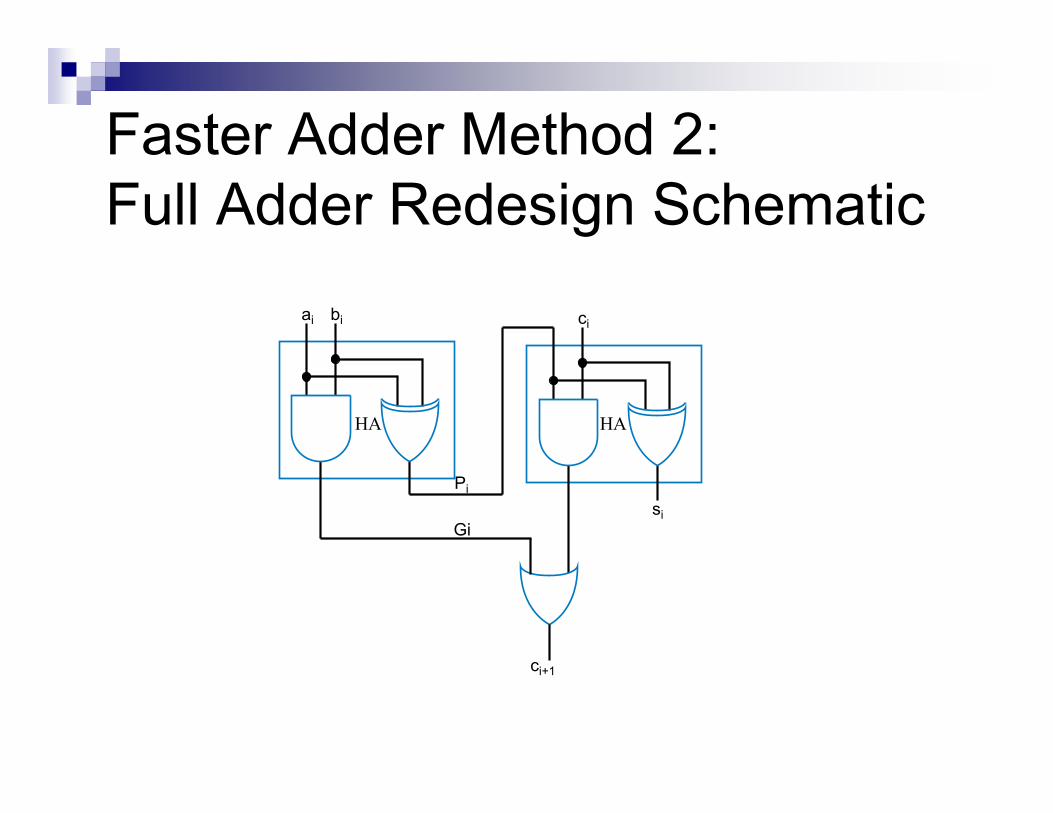
Faster Adder Method 2:
Full Adder Redesign Schematic
ai bi
Gi
HA
ci
ci+1
si
Pi
HA

썆 擰ɐ Ч
Faster Adder Method 2:
Carry-Lookahead Logic
� Using this newly redesigned Adder, we
can use the output of the first HA to
provide useful carry-ahead information.
�Pi is called the Carry Propagate
� This is asserted only when a the carry-in
propagates through this level.
�Gi is called Carry Generate
� This is asserted only when the addition of a & b will
generate a carry.
擰ʽ� Ч
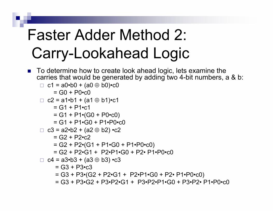
Faster Adder Method 2:
Carry-Lookahead Logic� To determine how to create look ahead logic, lets examine the
carries that would be generated by adding two 4-bit numbers, a & b:� c1 = a0•b0 + (a0 ⊕ b0)•c0
= G0 + P0•c0
� c2 = a1•b1 + (a1 ⊕ b1)•c1
= G1 + P1•c1
= G1 + P1•(G0 + P0•c0)
= G1 + P1•G0 + P1•P0•c0
� c3 = a2•b2 + (a2 ⊕ b2) •c2
= G2 + P2•c2
= G2 + P2•(G1 + P1•G0 + P1•P0•c0)
= G2 + P2•G1 + P2•P1•G0 + P2• P1•P0•c0
� c4 = a3•b3 + (a3 ⊕ b3) •c3
= G3 + P3•c3
= G3 + P3•(G2 + P2•G1 + P2•P1•G0 + P2• P1•P0•c0)
= G3 + P3•G2 + P3•P2•G1 + P3•P2•P1•G0 + P3•P2• P1•P0•c0

콆 蔐ɐ ь
Faster Adder Method 2:
Carry-Lookahead Adder Schematic
� The carry-propagate adder can now be redesigned:

退�
Faster Adder Method 2:
Iterative Carry-Lookahead Adder
� Carry-Lookahead has a problem� The Fan-In of gates in the carry-lookahead logic increases
as the number of bits increases.
� This can get unwieldy quickly.� 4 or 8 bits is reasonable
� The answer is an iterative structure.� Create smaller look-ahead adders
� Connect them together into a larger adders
� Example: Create a 16-bit adder from 4 carry-lookahead 4-bit adders in a ripple configuration.
� Is this a good enough design?
蔐ɐ� ь
Faster Adder Method 2:
Hierarchical Carry-Lookahead Adder
� Our initial optimization was aimed at
removing ripple carries E can we just
apply the same optimization again?
�YES!
�Create a second layer of carry-lookahead for
the iterative carry-lookahead adders.
� Creates a hierarchy of lookahead logic

�ʽ
Faster Adder Method 2:
Hierarchical Carry-Lookahead Adder
狰ɐ� ѡ
Faster Adder Method 3:
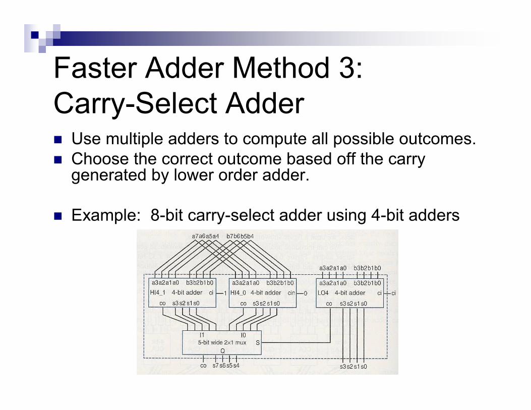
Carry-Select Adder� Use multiple adders to compute all possible outcomes.
� Choose the correct outcome based off the carry generated by lower order adder.
� Example: 8-bit carry-select adder using 4-bit adders

�ʽ
Faster Adder Tradeoff
Comparison
蔐ɐ� ь
Serial vs. Concurrent
Optimizations & Tradeoffs
� Many tradeoffs and optimizations simplify
to restructuring a design to take advantage
of either:
�Serialization
� Performing tasks one at a time
� Leads to smaller designs, but is slower
�Concurrancy
� Performing tasks in parallel
� Fast, but larger designs
⡆ʽ
Pipelining
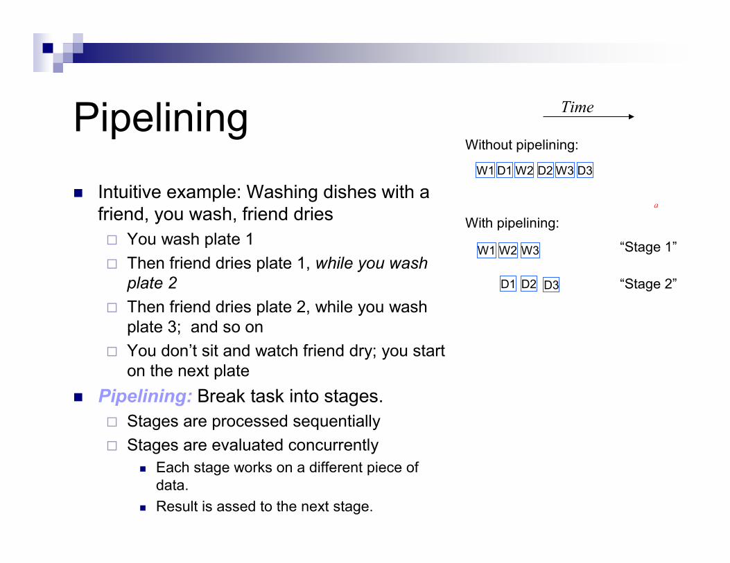
� Intuitive example: Washing dishes with a
friend, you wash, friend dries
� You wash plate 1
� Then friend dries plate 1, while you wash
plate 2
� Then friend dries plate 2, while you wash
plate 3; and so on
� You don’t sit and watch friend dry; you start
on the next plate
� Pipelining: Break task into stages.
� Stages are processed sequentially
� Stages are evaluated concurrently
� Each stage works on a different piece of
data.
� Result is assed to the next stage.
W1 W2 W3D1 D2 D3
Without pipelining:
With pipelining:
“Stage 1”
“Stage 2”
Time
W1
D1
W2
D2
W3
D3
a
f 蔐ɐ ь
Pipelining Example
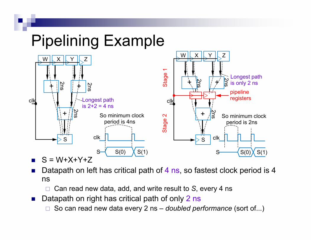
� S = W+X+Y+Z
� Datapath on left has critical path of 4 ns, so fastest clock period is 4 ns
� Can read new data, add, and write result to S, every 4 ns
� Datapath on right has critical path of only 2 ns
� So can read new data every 2 ns – doubled performance (sort of...)
W X Y Z
+ +
+
S
clk
Longest pathis only 2 ns
clk
S S(0)
So minimum clockperiod is 2ns
S(1)
clk
S S(0)
So minimum clockperiod is 4ns
S(1)
Longest pathis 2+2 = 4 ns
W X Y Z
+ +
+
S
clk
2ns
pipelineregisters
Sta
ge 1
Sta
ge 2
2ns
2ns
2ns
2ns
2ns
Pipelining Example
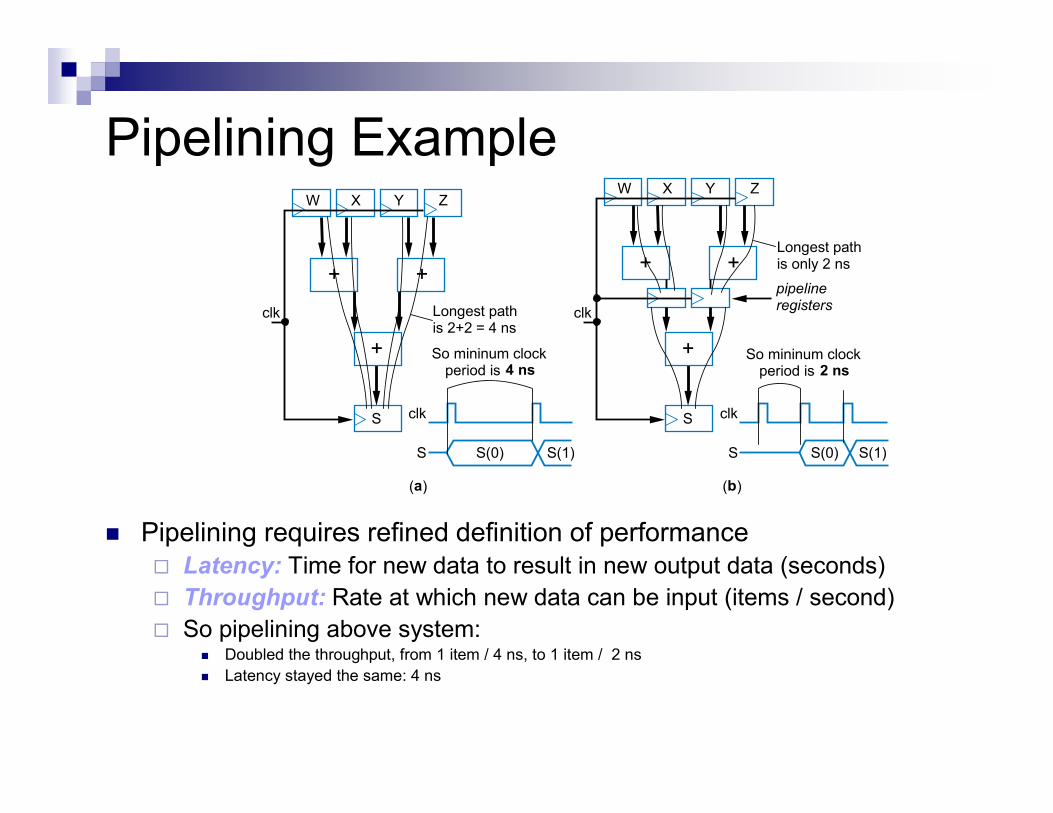
� Pipelining requires refined definition of performance
� Latency: Time for new data to result in new output data (seconds)
� Throughput: Rate at which new data can be input (items / second)
� So pipelining above system:� Doubled the throughput, from 1 item / 4 ns, to 1 item / 2 ns
� Latency stayed the same: 4 ns
W X Y Z
+ +
+
S
clk
clk
S S(0)
So mininum clockperiod is 4 ns
S(1)
Longest pathis 2+2 = 4 ns
W X Y Z
+ +
+
S
clk
clk
S S(0)
So mininum clockperiod is 2 ns
S(1)
Longest pathis only 2 ns
pipelineregisters
(a) (b)
ɐن
Concurrency
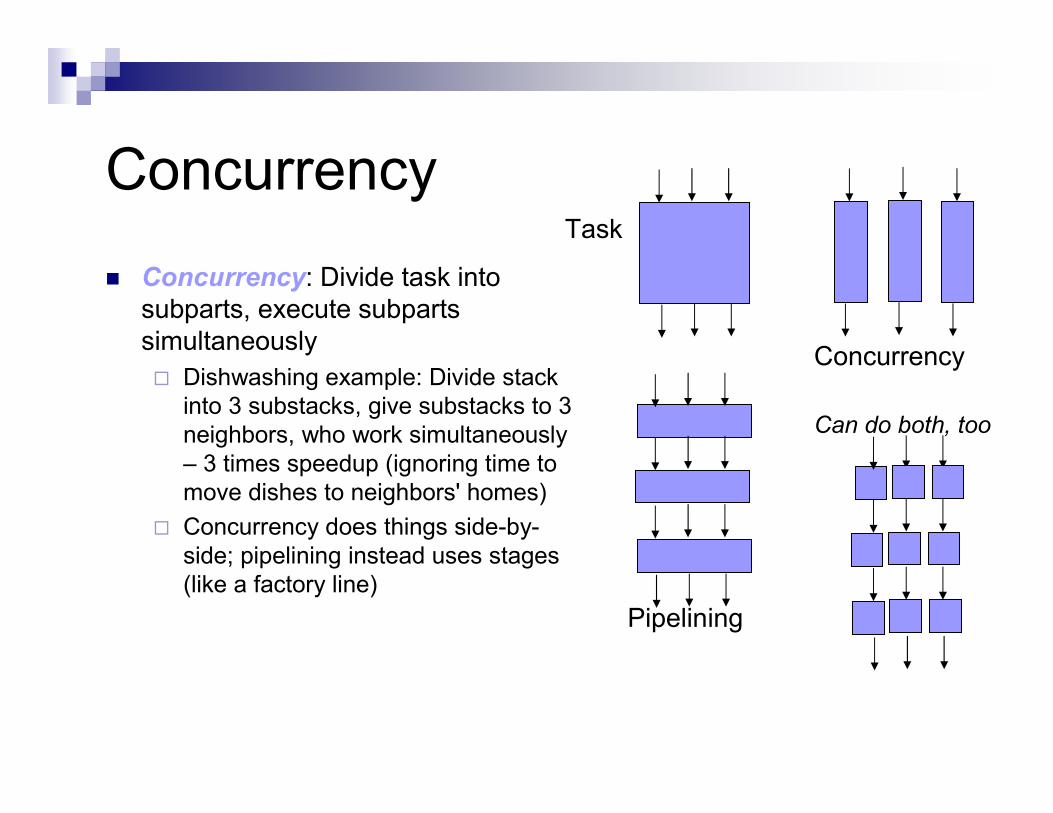
� Concurrency: Divide task into
subparts, execute subparts
simultaneously
� Dishwashing example: Divide stack
into 3 substacks, give substacks to 3
neighbors, who work simultaneously
– 3 times speedup (ignoring time to
move dishes to neighbors' homes)
� Concurrency does things side-by-
side; pipelining instead uses stages
(like a factory line)
Task
Pipelining
Concurrency
Can do both, too
㭆ʽ
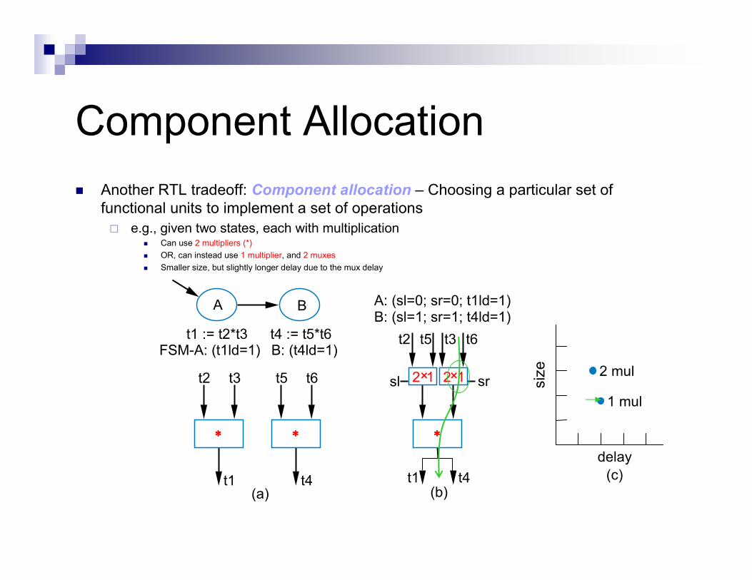
Component Allocation
� Another RTL tradeoff: Component allocation – Choosing a particular set of
functional units to implement a set of operations
� e.g., given two states, each with multiplication� Can use 2 multipliers (*)
� OR, can instead use 1 multiplier, and 2 muxes
� Smaller size, but slightly longer delay due to the mux delay
A B
t1 := t2*t3 t4 := t5*t6
∗∗∗∗
t2
t1
t3
∗∗∗∗
t5
t4
t6
(a)
FSM-A: (t1ld=1) B: (t4ld=1)
∗∗∗∗
2×1
t4t1(b)
2×1sl
t2 t5 t3 t6
sr
A: (sl=0; sr=0; t1ld=1)B: (sl=1; sr=1; t4ld=1)
(c)
2 mul
1 mul
delay
siz
e
ቆɐ
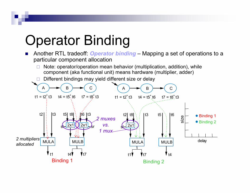
Operator Binding� Another RTL tradeoff: Operator binding – Mapping a set of operations to a
particular component allocation
� Note: operator/operation mean behavior (multiplication, addition), while component (aka functional unit) means hardware (multiplier, adder)
� Different bindings may yield different size or delay
Binding 2
A B
t1 = t2* t3 t4 = t5* t6 t7 = t8* t3
C A B
t1 = t2* t3 t4 = t5* t6 t7 = t8* t3
C
MULA MULB
2x1
t7t4
2x1
t5t3t2 t8 t6 t3
sr
t1
sl 2x1
t2 t8 t3
sl
t6t5
t7t1 t4
MULBMULA2 multipliers
allocated
Binding 1 Binding 2
Binding 1
delay
siz
e
2 muxes
vs.
1 mux

�б
22
Operator Scheduling� Yet another RTL tradeoff: Operator scheduling –
Introducing or merging states, and assigning operations
to those states.
*
t3t2
*
t1
t6t5
*
t4
B2
(someoperations)
(someoperations)
t1 = t2* t3t4 = t5* t6
A B C
*t4 = t5 t6
3-state schedule
delay
siz
e
2x1
t4t1
2x1
t2 t5 t3 t6
srsl
4-state schedule
smaller
(only 1 *)
but more
delay due to
muxes, and
extra state
a
A B
(someoperations)
(someoperations)
t1 = t2*t3t4 = t5*t6
C
�Ш
Optimization Level
� Typically, optimizations and tradeoffs made at higher design levels have a greater impact.� i.e. Changes made during the RTL design will
have much more effect than optimizing a gate design.
�High level algorithm changes can have a major effect on the size and speed of the circuit.� A classic example of algorithm selection is for search
algorithms� A binary search is much faster than a linear search.
�Lower level changes only serve to tune higher level changes.
但ʽ
Power Optimization & Tradeoffs
� Most power dissipation in a CMOS transistors occurs during switching.� Known as dynamic power
� P = k * CV2f � P � Power
� k � a constant for the transistor
� C � Capacitance of the transistor
� V � Voltage across the transistor
� f � Switching frequency
� Voltage and frequency are the two most easily modified parameters� Voltage
� Voltage reduction is desirable due to the quadratic contribution to power.
� Low voltage gates can be smaller, which also reduces capacitance
� Low power gates generally have longer delays.
� Frequency� Slower circuits switch less often and so burn less dynamic power
� This comes at the cost of performance.

甠Ш
Clock Gating
� Clock gating is a technique for disabling
sections of a circuit by preventing the
propagation of a clock signal.
�This is generally a bad idea as it can
introduce skew.
� If you are interested in this topic, read the
section on the book on p. 390.
Related Documents