Databases of surface wave dispersion - Home | Earth-prints

945

ANNALS OF GEOPHYSICS, VOL. 48, N. 6, December 2005

Key words seismic tomography – upper mantle –lateral resolution – azimuthal anisotropy

1. Introduction

Seismic surface waves are dispersive; theirspeed of propagation is a function of their fre-quency, or, in other words, individual harmoniccomponents of the surface wave seismogram(individual modes) propagate over the globe atdifferent speeds. For any given earthquake-seismometer couple, one can isolate from theseismogram each harmonic component, andmeasure its average speed (phase velocity) be-tween source and receiver. We call «dispersioncurve» a plot of average phase velocity against

frequency. From a large set of measured disper-sion curves, with sources and stations providingas uniform a coverage of the Earth as possible,local phase velocity heterogeneities can bemapped as a function of longitude and latitude.At each location, perturbations in phase veloci-ty with respect to a given reference model areweighted averages of seismic heterogeneities inthe underlying mantle (Jordan, 1978).

Through the steps outlined above, measure-ments of surface wave dispersion provide themost important global seismological constrainton the nature of the Earth’s upper mantle (e.g.,Ekström, 2000). Over the last decades, two largeintermediate-period (35-150 s) fundamentalmode dispersion databases have been assembledby Trampert and Woodhouse (1995, 2001) andEkström et al. (1997) from global networks ofbroadband seismic stations, and are now avail-able to the public. Both are currently employedin global tomography studies (e.g., Boschi andEkström, 2002; Spetzler et al., 2002; Antolik et al., 2003; Beghein, 2003; Boschi et al., 2004;

Databases of surface wave dispersion

Simona Carannante (1) and Lapo Boschi (2)(1) Istituto Nazionale di Geofisica e Vulcanologia, Sede di Bologna, Italy

(2) ETH, Zurich, Switzerland

Abstract Observations of seismic surface waves provide the most important constraint on the elastic properties of the Earth’slithosphere and upper mantle. Two databases of fundamental mode surface wave dispersion were recently compiledand published by groups at Harvard (Ekström et al., 1997) and Utrecht/Oxford (Trampert and Woodhouse, 1995,2001), and later employed in 3-d global tomographic studies. Although based on similar sets of seismic records,the two databases show some significant discrepancies. We derive phase velocity maps from both, and comparethem to quantify the discrepancies and assess the relative quality of the data; in this endeavour, we take careful ac-count of the effects of regularization and parametrization. At short periods, where Love waves are mostly sensitiveto crustal structure and thickness, we refer our comparison to a map of the Earth’s crust derived from independentdata. On the assumption that second-order effects like seismic anisotropy and scattering can be neglected, we findthe measurements of Ekström et al. (1997) of better quality; those of Trampert and Woodhouse (2001) result inphase velocity maps of much higher spatial frequency and, accordingly, more difficult to explain and justify geo-physically. The discrepancy is partly explained by the more conservative a priori selection of data implemented byEkström et al. (1997). Nevertheless, it becomes more significant with decreasing period, which indicates that itcould also be traced to the different measurement techniques employed by the authors.

Mailing address: Dr. Simona Carannante, Istituto Nazio-nale di Geofisica e Vulcanologia, Sede di Bologna, Via D.Creti 12, 40128 Bologna, Italy; e-mail: [email protected]

946

Simona Carannante and Lapo Boschi

Boschi, 2005); their accuracy becomes evenmore important when they are used to constrainobservables that are inherently hard to resolve,like the azimuthal anisotropy of surface wavepropagation (Laske and Masters, 1998; Beckeret al., 2003; Trampert and Woodhouse, 2003).Boschi and Woodhouse (2005) point to the sub-stantial disagreement between published globalmodels of surface wave anisotropy, and the needto explain it partly motivates the present study.

The Utrecht and Harvard databases are ingood, but not complete agreement; it has beenobserved by their authors, and we again illustratebelow, that those of Trampert and Woodhouse(1995, 2001) require phase velocity maps with awhiter spectrum than those of Ekström et al.(1997), to be explained comparably well. Thisdiscrepancy might depend on the a priori selec-tion of globally recorded seismic records in thetwo studies: Ekström et al. (1997) obtained phasevelocities from digital seismograms from theGlobal Seismographic Network (GSN), usingearthquake sources between 1989 and 1995,Trampert and Woodhouse (1995, 2001) used dig-ital GDSN and GEOSCOPE seismograms recordedbetween 1980 and 1990. The discrepacy couldalso arise from the differences in the measure-ment algorithm designed and employed by thetwo groups. In both cases theoretical («synthet-ic») seismograms are calculated from theoreticaldispersion curves, and compared to the measuredone. An inverse problem is then solved to find thetheoretical dispersion curve that minimizes themisfit between measured and synthetic seismo-grams. Such optimal dispersion curve is the dis-persion measurement sought. As we shall illus-trate below, the two groups implemented thisprocedure in different ways.

Thus far, 2-d phase velocity and 3-d shearvelocity maps have been derived independent-ly from the two databases by different authors,making use of different tomographic algo-rithms; Ritzwoller et al. (2001) and Shapiroand Ritzwoller (2002) merged all data in a sin-gle set that they inverted, but did not provide acomparative analysis of data quality.

We present two sets of phase velocity maps,derived independently from the two databases,with the same parameterization, inversion algo-rithm and regularization scheme. At the period

where discrepancies are most severe (35 s Lovewaves), we refine the parameterization and ex-plore the solution space, in an attempt to deter-mine whether Trampert and Woodhouse’s (2001)database can indeed resolve coherent isotropicheterogeneities of high spatial frequency.

2. Measuring surface wave dispersion

Following Ekström et al.’s (1997) notation,we write a surface wave seismogram u(ω) inthe form

(2.1)

where amplitude A and phase Φ are functionsof frequency ω. Φ(ω) and the phase velocityc(ω) are related

(2.2)

with X denoting propagation path length meas-ured along the great circle. u (ω) can be calcu-lated, e.g., by surface wave JWKB theory as de-scribed by Tromp and Dahlen (1992, 1993).

Given an observed seismogram, surface wavedispersion between the corresponding source andreceiver is measured by finding the curves A(ω)and c(ω) (hence Φ(ω)) that minimize the misfitbetween the observed seismogram and u(ω). Thebest-fitting c(ω) is the seeked dispersion curve.

Ekström et al. (1997) and Trampert andWoodhouse (1995, 2001) find synthetic seis-mograms in slightly different, but equivalent,ways. Both groups write the corrections to am-plitude and phase, with respect to PREM (Dzie-wonski and Anderson, 1981), as linear combi-nations of a set of cubic splines f i(ω), with co-efficients bi and di, respectively,

(2.3)

(2.4)

and the dispersion measurement is reduced tothe determination of bi, di (i=1, ..., N).

The outlined inverse problem is highly non-linear. Ekström et al. (1997) accordingly choseto solve it through the non-linear SIMPLEX

( ) ( )fc di i

i

N

1

=d ~ ~=

/

( ) ( )A b fi i

i

N

1

=d ~ ~=

/

( )( )cX

=~ ~~Φ

( ) ( )u A e ( )Φi=~ ~ ~


method (e.g., Press et al., 1994). They parame-terized their dispersion curves in terms of onlyN=6 splines; this number being relativelysmall, the curves tend to be smooth and no fur-ther regularization is needed.

Conversely, Trampert and Woodhouse (1995,2001) described dispersion curves as linear com-binations of as many as N=36 splines. They ac-comodated the nonlinearity of the inverse prob-lem by first measuring group velocities, whichare «secondary observables easily calculated bythe seismograms». They then derived phase ve-locity dispersion curves from them, through thenonlinear least-squares algorithm of Tarantolaand Valette (1982), regularized by some rough-ness damping constraint.

The main reason for requiring dispersioncurves to be smooth, is to avoid fictitious fluc-tuations due to «2π» ambiguity: notice from eq.(2.1) that the surface wave seismogram is a pe-riodic function of Φ with period 2π ; when dis-persion is measured, values of Φ different ofexactly 2π will provide an equally good fit tothe data; and perturbations δΦ larger than 2πcannot simply be discarded, because at short to intermediate periods (say, <100 s), hetero-geneities in the Earth’s structure can suffice tocause phase anomalies of more than one cycle.Both groups solved this ambiguity requiring thedispersion curve to be smooth (see, e.g., fig. 2of Trampert and Woodhouse, 1995); Ekström et al. (1997) noted that at longer periods (>100s) a phase measurement can be associated witha total cycle count with no difficulty; theytherefore preferred to first measure dispersionin the longer period range, and extend themeasured dispersion curve to shorter period ina subsequent step, with the requirement that itbe smooth, as they illustrated in their fig. 3.

3. Phase velocity maps

3.1. Intermediate resolution maps at different periods

We derive Love and Rayleigh wave phasevelocity maps at all periods (35 to 150 s) wheremeasurements are available; a separate tomo-graphic inversion is performed at each period to

find an independent phase velocity map; wethen compare maps obtained from Trampertand Woodhouse’s (2001) database with thoseobtained from Ekström et al.’s (1997). Bothdatabases have, at all periods, a relatively goodcoverage of the entire globe. We employ, inboth cases, the same tomographic parameteri-zation (approximately equal area pixels, of size5°×5° degree at the equator), regularization (acombination of norm and roughness damping),and inversion algorithm (LSQR) (Boschi andDziewonski, 1999; Boschi, 2001): differencesbetween the maps must then arise from discrep-ancies in the data. The regularization schemewas chosen after a number of preliminary in-versions (Carannante, 2004).

The phase velocity distributions that wefound share the general character of alreadypublished maps. For any given regularizationscheme, inversions of Harvard data lead to asystematically higher variance reduction thanthose of Utrecht ones, also confirming pub-lished results.

The correlation between maps improves withincreasing period, and is systematically higher forRayleigh, with respect to Love waves. Figure 1allows a visual comparison between Love andRayleigh wave velocity as imaged from the twodatabases, at short (35 s) and intermediate (∼75 s)periods. In fig. 2, we show the harmonic spectraof the same images, derived as described, e.g., byBoschi and Dziewonski (1999). The agreementbetween the images is remarkably good at ∼75-80 s, both in the spatial and frequency domains(comparing the third and fourth panels of fig. 2,one might notice that, as anticipated, theRayleigh wave spectra are slightly more similarto each other than the Love wave ones); high cor-relation between images based on the Trampertand Woodhouse’s (2001) and Ekström et al.’s(1997) databases is confirmed at all measured in-termediate and long periods (Carannante, 2004).

As period decreases, a loss of correlation isevident; it is maximum at 35 s (measurementsat shorter periods are not provided in the data-bases), both for Love and Rayleigh waves, butstronger in the case of Love waves. The 35 sLove wave maps disagree most evidently in theregions of thickest crust (Andes, Tibet), whereEkström et al.’s (1997) data provide a much

947

948


lower phase velocity than those of Trampertand Woodhouse (2001). The top panels of fig. 2show that the discrepancy has a global charac-ter, with the former images being characterizedby a much redder spectrum than the latter.

3.2. Higher resolution, short-period phasevelocity maps

The exercise described in the previous sec-tion confirms that a discrepancy exists betweenthe databases in question. The discrepancy ispractically negligible at intermediate to long

periods, but becomes more severe with decreas-ing period. In a short-period regime, tomo-graphic inversions of the two databases result inphase velocity maps that would have, at least incertain regions, quite different implications onthe properties of the upper mantle.

To investigate the nature of the discrepancy,we focus our attention on Love wave observa-tions at 35 s, where the most evident disagree-ment is found. We refine our grid, reducing thepixel size to 2°×2° at the equator; this parame-terization, involving ∼10000 free parameters,should be sufficient to resolve any short-wave-length structure «seen» by the data. This is an

Fig. 1. Percent perturbations in phase velocity with respect to PREM, derived from Trampert and Woodhouse’s(2001) (left) and Ekström et al.’s (1997) (right) databases. For each database, the results of inverting four inde-pendent subsets are shown: Love waves at 35 s (top), Rayleigh waves at 35 s (middle, top), Love waves at 75 s(Harvard) or 79 s (Utrecht) (middle, bottom), Rayleigh waves at 75 s (Harvard) or 78 s (Utrecht) (bottom).


important issue: if either database contains in-formation on the structure of very high harmon-ic degree, that a 5°×5° grid cannot represent,aliasing of this signal could in principle be areason for discrepancies between images.

We must likewise rule out the possible inad-equacy of regularization as a reason for discrep-ancy: we repeat our inversions with a number ofdifferent regularization schemes. A few exam-ples are shown in fig. 3; at each damping level,the phase velocity distributions derived from thetwo databases differ, with a pattern similar to thatoutlined by our lower resolution inversions. Thespectral plots of fig. 4 are also qualitatively con-sistent with those in the top panel of fig. 2, ex-cept for the obviously underdamped case (normand roughness damping parameters equal to0.005), where the large l harmonic coefficientsclearly take non-physical values.

The most outstanding difference betweenmaps derived from Ekström et al.’s (1997) andTrampert and Woodhouse’s (2001) databases isfound, again, in regions of anomalously thickcrust. Regardless of regularization scheme andparameterization, Tibet and Andes are coherent-ly slow according to the former database, local-ly fast according to the latter. We compare theresults of our inversions with a theoretical 35 sLove wave phase velocity map (bottom of fig.3), computed, following Boschi and Ekström(2002), from a spherically symmetric mantlemodel combined with the laterally heteroge-neous crustal model Crust-2.0 (Bassin et al.,2000) derived from observations entirely inde-pendent from the ones discussed here. This sim-plified model favours uniformly low phase ve-locity at Tibet and Andes; for Trampert andWoodhouse’s (2001) observations to be correct,shear velocity then has to be very high in theupper mantle underlying those regions (see,e.g., Boschi and Ekström, 2002, fig. 7), while asimpler mantle model would be sufficient to ex-plain Ekström et al.’s (1997) data.

Given the systematic nature of the discrepan-cy, always stronger in regions of thick crust, wecould infer that either shorter-period signal (moresensitive to crustal thickness) «leaks» into the 35 s Love wave measurements of Ekström et al.(1997), or longer-period signal (more sensitive toupper mantle structure) «leaks» into Trampert

949

Fig. 2. Spherical harmonic spectra of the maps fromfig. 1. The spectra of maps derived from Utrecht dataare plotted in grey; the black curves are the spectra ofthe corresponding maps, derived from Harvard data.

950


and Woodhouse’s (2001). Figure 5, where weshow correlation between maps at a set of neigh-bouring periods, is to some extent consistent withthe latter hypothesis, while the former cannot betested in the absence of global maps of phase ve-

locity at shorter periods. In both cases, discrepan-cies would be ascribed to faults in the measure-ment algorithms.

The high spatial frequency character of mapsderived, at this period, from Trampert and Wood-

Fig. 3. Love wave dispersion data at 35 s, from both Trampert and Woodhouse’s (2001) (left) and Ekström et al.’s (1997) (right) databases, are inverted with four different regularization schemes. Roughness and Normdamping parameters, always coincident in this experiment, are given to the left of each couple of maps. The bot-tom panel shows a theoretical 35 s Love phase velocity map: at each pixel of Crust-2.0, local mode eigenfunc-tions were used to calculate the phase velocity resulting from a spherically symmetric mantle and heterogeneouscrust. We do not expect tomographic and theoretical maps to concide, but they should share some prominent fea-tures. The colour scale is the same as in fig. 1.


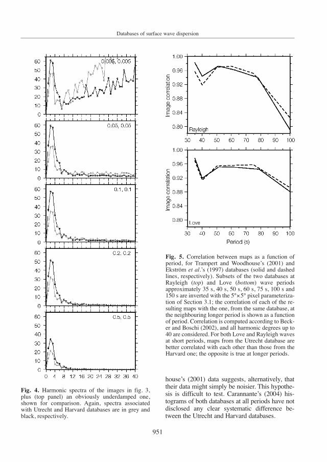
house’s (2001) data suggests, alternatively, thattheir data might simply be noisier. This hypothe-sis is difficult to test. Carannante’s (2004) his-tograms of both databases at all periods have notdisclosed any clear systematic difference be-tween the Utrecht and Harvard databases.

951

Fig. 4. Harmonic spectra of the images in fig. 3,plus (top panel) an obviously underdamped one,shown for comparison. Again, spectra associatedwith Utrecht and Harvard databases are in grey andblack, respectively.

Fig. 5. Correlation between maps as a function ofperiod, for Trampert and Woodhouse’s (2001) andEkström et al.’s (1997) databases (solid and dashedlines, respectively). Subsets of the two databases atRayleigh (top) and Love (bottom) wave periods approximately 35 s, 40 s, 50 s, 60 s, 75 s, 100 s and150 s are inverted with the 5°×5° pixel parameteriza-tion of Section 3.1; the correlation of each of the re-sulting maps with the one, from the same database, atthe neighbouring longer period is shown as a functionof period. Correlation is computed according to Beck-er and Boschi (2002), and all harmonic degrees up to40 are considered. For both Love and Rayleigh wavesat short periods, maps from the Utrecht database arebetter correlated with each other than those from theHarvard one; the opposite is true at longer periods.

952


In principle, scattering and anisotropy insurface wave propagation are possible causesfor aliasing and subsequent discrepancies be-tween databases: an accurate dispersion meas-urement could contain, for example, a coherent«aniso-tropic signal» that might have beenwrongly removed in a less accurate one. Scat-tering and anisotropic effects are also period-dependent. Again, we are not yet capable oftesting this hypothesis; attempts at mapping theazimuthal anisotropy of surface wave phase ve-locity have not led to consistent results (Laskeand Masters, 1998; Becker et al., 2003; Tram-pert and Woodhouse, 2003; see also Boschi andWoodhouse, 2005 for a comparison); Boschi(2005) notes that accounting for scattering ef-fects in inversions of the Harvard database ap-pears to lead to an effective improvement inresolution, but, at the present stage, his resultsare only preliminary.

3.3. Further exploration of the solution space

We find the «L-curves» (e.g., Hansen, 1998)associated with the Love wave 35 s, 2°×2° pix-els inverse problem (Section 3.2): in fig. 6 (top)data misfit (1-variance reduction) is plotted as afunction of total roughness (eq. 2.21 of Boschi,2001), for a number of phase velocity maps de-rived from the Utrecht (solid lines) and Harvard(dashed lines) databases, with roughness mini-mization as the only damping constraint. Rough-ness minimization, with respect to other damp-ing schemes, limits the effect of the startingmodel on the final solution (e.g., Inoue et al.,1990, Section 3.3.1 and fig. 2). Values of theroughness damping parameter range from 0.005(minimum misfit) to 0.5 (maximum misfit). Wealso take the derivative of misfit with respect tototal image roughness (fig. 6, bottom), to makethe two L-curves comparable.

If a small increase in image complexity is suf-ficient to reduce the misfit significantly, one mustinfer that meaningful signal is being mapped, andthat the image resolution is also being improved.Conversely, if misfit remains approximately con-stant even for large increases in total roughness,the regularization must be inadequate, so that theeffect of noise in the data, and of subsequent nu-

merical instabilities, become prominent in the so-lution. Ideally, the vertex of the «L»’s in curveslike those of fig. 6 should identify the optimalvalues of total roughness and damping parameter,leading to the lowest possible misfit while mini-mizing the fictitious mapping of noise.

The L-shape of the curves in fig. 6 indicatesthat the data are of sufficiently high quality toresolve meaningful Earth structure; it is hard,however, to identify an optimal value for thedamping parameter, as the high-resolution gridemployed here is probably fine enough to allowa certain amount of noise to be mapped into fic-titious phase velocity heterogeneity. The curvestake a more pronounced L-shape in the case of

Fig. 6. L-curves (e.g., Hansen, 1998) associatedwith the Harvard (dashed lines) and Utrecht (solidlines) databases. The image roughness is defined asby Boschi (2001, Section 2.2.1) or Trampert andWoodhouse (1995, eq. (21)). Misfit is defined as 1minus the variance reduction.

953


Harvard data, easier to explain in terms ofisotropic phase velocity variations.

After numerous independent inversions ofboth 35 s Love wave databases, we show in figs.7 (Harvard) and 8 (Utrecht) variance reductionas a function of norm and roughness dampingparameter. We achieve a systematically better fitof Harvard data, with respect to Utrecht ones, re-gardless of the regularization. Consistently withthe simple shape of the curves in fig. 6, we findthat variance reduction decreases monotonicallywith increasing damping parameters.

We conclude that the analysis of Section 3.2holds true independently of the chosen dampingparameters.

4. Conclusions

We confirm that a discrepancy exists be-tween Ekström et al.’s (1997) and Trampert andWoodhouse’s (1995, 2001) measurements ofteleseismic surface wave dispersion. At long pe-riods, it only concerns the short spatial frequen-cy component of imaged phase velocity, while atshort periods the discrepancy is significant at allharmonic degrees (figs. 1 and 2 above).

We have investigated the nature of this dis-crepancy, deriving independent, isotropic, glob-al phase velocity maps from both databases, forboth Love and Rayleigh waves at all availableperiods.

A preliminary set of inversions, with a para-meterization of intermediate nominal resolution(5°×5°), shows that the Harvard data are fit sys-tematically better than the Utrecht ones. Thiseffect could be explained in various ways. TheHarvard measurements might simply be cleaner,either because Ekström et al.’s (1997) algorithmis more accurate than Trampert and Wood-house’s (1995, 2001), or because the Harvardgroup started with a set of seismograms of high-er quality. Alternatively, the Utrecht databasemight have higher sensitivity to small-scalestructure, damped out from Ekström et al.’s(1997) measurements, and not resolved by agrid of 5°×5° pixels.

Having repeated our analysis with a muchfiner (2°×2°) parameterization, and with a widespectrum of regularization schemes (figs. 3 and

Fig. 8. Variance reduction of 35 s Love wave disper-sion from the Utrecht database, as a function of norm(x-axis) and roughness (y-axis) damping parameters.

Fig. 7. Inversions of the 35 s Love wave Harvarddatabase: variance reduction as a function of norm(x-axis) and roughness (y-axis) damping parameters.

954


4; figs. 6 through 8), we can rule out the latterspeculation: the increase in nominal resolutionhas not affected the nature of the discrepancy be-tween images based on Utrecht versus Harvarddata, nor the systematic difference in data-fit.

We have, however, neglected anisotropyand scattering; while it is very likely that theireffect be only minor, it is possible that modelsof phase velocity propagation including az-imuthal anisotropy (Laske and Masters, 1998;Becker et al., 2003; Trampert and Woodhouse,2003), and accounting for the effects of scatter-ing on data sensitivity (e.g., Spetzler et al.,2002) are significantly different, in theirisotropic component from the ones presentedhere. This issue calls for further work.

An additional explanation for the discrepan-cy in question could be a leakage of signalwhen dispersion is measured between neigh-boring surface wave periods. Figure 2 suggeststhat this effect might be severe enough, inTrampert and Woodhouse’s (2003) algorithm,to cause the Moho anomalies of Tibet and An-des (to which short period Love wave should bestrongly sensitive) to be missed. This specula-tion will need to be substantiated by bench-marking the two algorithms with each other.

Acknowledgements

We are particularly grateful to Prof. PaoloGasparini for his help and encouragement.Thanks also to Göran Ekström, Domenico Gia-rdini, Gabi Laske, Andrea Morelli, Jeroen Rit-sema, Jeannot Trampert, Aldo Zollo. The com-ments of Maurizio Bonafede and two anony-mous reviewers helped us improve the originalmanuscript. During his stay at Università diNapoli, Lapo Boschi was funded by Ministerodell’Istruzione, Università e Ricerca. All fig-ures were done with GMT (Wessel and Smith,1991). Our research benefits from the EuropeanUnion SPICE research and training network.

REFERENCES

ANTOLIK, M., Y.J. GU, G. EKSTRÖM and A.M. DZIEWONSKI

(2003): J362D28: a new joint model of compressional

and shear velocity in the mantle, Geophys. J. Int., 153,443-466.

BASSIN, C., G. LASKE and G. MASTERS (2000): The currentlimits of resolution for surface wave tomography inNorth America, EOS, Trans. Am. Geophys. Un., 81,F897.

BECKER, T.W. and L. BOSCHI (2002): A comparison of to-mographic and geodynamic mantle models, Geochem.Geophys. Geosys., 3, 2001GC000168.

BECKER, T.W., J.B. KELLOGG, G. EKSTRÖM and R.J. O’CON-NELL (2003): Comparison of azimuthal seismic ani-sotropy from surface waves and finite strain from glob-al mantle-circulation models, Geophys. J. Int., 155,696-714.

BEGHEIN, C. (2003): Seismic anisotropy inside the Earthfrom a model space search approach, Ph.D. Thesis,(Utrecht University, Utrecht, Netherlands).

BOSCHI, L. (2001): Applications of linear inverse theory inmodern global seismology, Ph.D. Thesis (Harvard Uni-versity, Cambridge, Massachusetts).

BOSCHI, L. (2005): Global multi-resolution models of sur-face wave propagation: the effects of scattering, Geo-phys. J. Int. (submitted).

BOSCHI, L. and A.M. DZIEWONSKI (1999): «High» and «low»resolution images ofthe Earth’s mantle-Implications ofdifferent approaches to tomographic modeling, J. Geo-phys. Res., 104, 25,567-25,594.

BOSCHI, L. and G. EKSTRÖM (2002): New images of theEarth’s upper mantle from measurements of surface-wave phase velocity anomalies, J. Geophys. Res., 107,doi: 10.129/2000JB000059.

BOSCHI, L. and J.H. WOODHOUSE (2005): Surface wave ray-tracing and azimuthal anisotropy, Geophys. J. Int. (inpress).

BOSCHI, L., G. EKSTRÖM and K. KUSTOWSKI (2004): Multi-ple resolution surface wave tomography: the Mediter-ranean Basin, Geophys. J. Int., 157, 293-304, doi:10.1111j.1365-246X.2004.02194.x.

CARANNANTE, S. (2004): Velocità di fase delle onde sis-miche di superficie: immagini tomografiche globali arisoluzione variabile, Tesi di Laurea (Università degliStudi di Napoli «Federico II», Napoli, Italy).

DZIEWONSKI, A.M. and D.L. ANDERSON (1981): Preliminaryreference Earth model, Phys. Earth Planet. Int., 25,297-356.

EKSTRÖM, G. (2000): Mapping the lithosphere and as-thenosphere with surface waves: lateral structure andanisotropy, in The History and Dynamics of GlobalPlate Motions, edited by M. RICHARDS, R.G. GORDON,and R.D. VAN DER HILST, Am. Geophys. Un. Monogr.,121, pp. 239.

EKSTRÖM, G., J. TROMP and E.W.F. LARSON (1997): Mea-surements and global models of surface wave propaga-tion, J. Geophys. Res., 102, 8137-8157.

HANSEN, P.C. (1992): Analysis of discrete ill-posed problemsby means of the L-curve, SIAM Rev., 34 (4), 561-580.

INOUE, H., Y. FUKAO, K. TANABE and Y. OGATA (1990):Whole mantle P-wave travel time tomography, Phys.Earth Planet. Int., 59, 294-328.

JORDAN, T.H. (1978): A procedure for estimating lateral-variations from low-frequency eigenspectra data, Geo-phys. J. R. Astron. Soc., 52, 441-455.

LASKE, G. and G. MASTERS (1998): Surface wave polariza-

955


tion data and global anisotropic structure, Geophys. J.Int., 132, 508-520.

PRESS, W.H., S.A. TEUKOLOSKY, W.T. VETTERLING and B.P.FLANNERY (1994): Numerical Recipes in FORTRAN

(Cambridge University Press, U.K.). RITZWOLLER, H., N.M. SHAPIRO, L.L. ANATOLI and M.L.

GARRETT (2001): CRUstal and upper mantle structurebeneath Antartica and surrounding oceans, J. Geophys.Res., 106, 30645-30670.

SHAPIRO, M.N. and M.H. RITZWOLLER (2002): Monte-Car-lo inversion for a global shear-velocity model of thecrust and upper mantle, J. Geophys. Res., 151, 88-105.

SPETZLER, J., J. TRAMPERT and R. SNIEDER (2002): The ef-fect of scattering in surface wave tomography, Geo-phys. J. Int., 149, 755-767.

TARANTOLA, A. and B. VALETTE (1982): Generalized non-linear inverse problems solved using the least-squarescriterion, Rev. Geophys. Space Phys., 20, 219-232.

TRAMPERT, J. and J.H. WOODHOUSE (1995): Global phasevelocity maps of Love and Rayleigh waves between 40and 150 s, Geophys. J. Int., 122, 675-690.

TRAMPERT, J. and J.H. WOODHOUSE (2001): Assessment ofglobal phase velocity models, Geophys. J. Int., 144,165-174.

TRAMPERT, J. and J.H. WOODHOUSE (2003): Global ani-sotropic phase velocity maps for fundamental modesurface waves between 40 and 150 s, Geophys. J. Int.,154, 154-165.

TROMP, J. and F.A. DAHLEN (1992): Variational principlesfor surface wave propagation on a laterally heteroge-neous Earth, II. Frequency domain JWKB theory, Geo-phys. J. Int., 109, 599-619.

TROMP, J. and F.A. DAHLEN (1993): Maslov theory for sur-face wave propagation on a laterally heterogeneousEarth, Geophys. J. Int., 115, 512-528.

WESSEL, P. and W.H.F SMITH (1991): Free software helpsmap and display data, EOS, Trans. Am. Geophys. Un.,72, 445-446.

(received January 28, 2005;accepted November 8, 2005)

Databases of surface wave dispersion - Home | Earth-prints

Documents