Database Visualisation Athanasios Kaliakoudas T H E U N I V E R S I T Y O F E D I N B U R G H Master of Science Computer Science School of Informatics University of Edinburgh 2011

Welcome message from author
This document is posted to help you gain knowledge. Please leave a comment to let me know what you think about it! Share it to your friends and learn new things together.
Transcript

Database Visualisation
Athanasios Kaliakoudas
TH
E
U N I V E RS
IT
Y
OF
ED I N B U
RG
H
Master of Science
Computer Science
School of Informatics
University of Edinburgh
2011

Abstract
This project is an attempt to deliver a database visualisation system; a new, user friendly way
of handling all the information stored in databases. The main objective is to create a solid
infrastructure that can connect to a given relational database and represent any dataset in a
clear and concise way. The infrastructure generates a visualization through which the user
can perform simple actions over the data. The system helps, thus, people that are not really
familiar with the SQL language (currently used in Database Management Systems) to perform
basic operations over sets of data in a fast, reliable and easily comprehensible way.
The system that is presented, although quite different from the usual approaches of database
visualisation such as graphs and treemaps, manages to perform well even in large databases
with many tables. It gives the user the ability to explore a database and perform, visually,
simple queries that translate to SELECT - FROM - WHERE queries in SQL.
To evaluate the system built on its usefulness, performance and reliability several tests and ex-
periments were conducted. For proof of usefulness, specific scenarios where created that users
had to go through; these scenarios showed that our implementation is very useful, as one most
occasions it is faster for a user to perform a task with our tool, rather than a Database Manage-
ment System. The system was also thoroughly tested with the use of quantitative methods to
make sure that performance issues or potential existence of bugs would not discourage people
from using it.
iii

Acknowledgements
I would like to thank my supervisor Dr. Stratis Viglas for supporting and guiding me throughout
the project. Also, I would like to thank my colleagues and friends who helped me evaluate the
system built. Finally, my family for their moral and financial support.
iv

Declaration
I declare that this thesis was composed by myself, that the work contained herein is my own
except where explicitly stated otherwise in the text, and that this work has not been submitted
for any other degree or professional qualification except as specified.
(Athanasios Kaliakoudas)
v

To Joanna.
vi
Table of Contents
List of Figures ix
List of Tables xi
1 Introduction 1
1.1 Overview . . . . . . . . . . . . . . . . . . . . . . . . . . . . . . . . . . . . . 2
1.2 Related Work . . . . . . . . . . . . . . . . . . . . . . . . . . . . . . . . . . . 3
1.2.1 History of Information Visualisation . . . . . . . . . . . . . . . . . . . 3
1.2.2 Database Visualisation . . . . . . . . . . . . . . . . . . . . . . . . . . 5
1.2.3 Current Database Visualisation tools . . . . . . . . . . . . . . . . . . . 8
1.3 Goals . . . . . . . . . . . . . . . . . . . . . . . . . . . . . . . . . . . . . . . 11
1.4 Motivation . . . . . . . . . . . . . . . . . . . . . . . . . . . . . . . . . . . . . 12
1.5 Assumptions . . . . . . . . . . . . . . . . . . . . . . . . . . . . . . . . . . . 12
2 System Design and features 15
2.1 Tools and libraries used . . . . . . . . . . . . . . . . . . . . . . . . . . . . . . 16
2.1.1 Processing . . . . . . . . . . . . . . . . . . . . . . . . . . . . . . . . 16
2.1.2 Microsoft SQL Server . . . . . . . . . . . . . . . . . . . . . . . . . . 17
2.1.3 JDBC . . . . . . . . . . . . . . . . . . . . . . . . . . . . . . . . . . . 17
2.1.4 Xampp . . . . . . . . . . . . . . . . . . . . . . . . . . . . . . . . . . 17
2.1.5 JarSigner . . . . . . . . . . . . . . . . . . . . . . . . . . . . . . . . . 18
2.1.6 NetBeans IDE . . . . . . . . . . . . . . . . . . . . . . . . . . . . . . 18
2.2 System features . . . . . . . . . . . . . . . . . . . . . . . . . . . . . . . . . . 18
2.2.1 Opening the program . . . . . . . . . . . . . . . . . . . . . . . . . . . 19
2.2.2 Relationship Mode . . . . . . . . . . . . . . . . . . . . . . . . . . . . 20
2.2.3 Zoom Mode . . . . . . . . . . . . . . . . . . . . . . . . . . . . . . . . 21
2.2.4 The results . . . . . . . . . . . . . . . . . . . . . . . . . . . . . . . . 22
3 Implementation 25
3.1 Database Connection . . . . . . . . . . . . . . . . . . . . . . . . . . . . . . . 26
vii
3.1.1 The connection . . . . . . . . . . . . . . . . . . . . . . . . . . . . . . 26
3.1.2 Metadata Extraction . . . . . . . . . . . . . . . . . . . . . . . . . . . 27
3.2 Allocating the tables to sketches . . . . . . . . . . . . . . . . . . . . . . . . . 30
3.3 The Graphical User Interface . . . . . . . . . . . . . . . . . . . . . . . . . . . 31
3.3.1 The frame . . . . . . . . . . . . . . . . . . . . . . . . . . . . . . . . . 31
3.3.2 The Sketches . . . . . . . . . . . . . . . . . . . . . . . . . . . . . . . 33
3.3.3 The Tables . . . . . . . . . . . . . . . . . . . . . . . . . . . . . . . . 35
3.3.4 The Columns . . . . . . . . . . . . . . . . . . . . . . . . . . . . . . . 37
3.3.5 The Results Area . . . . . . . . . . . . . . . . . . . . . . . . . . . . . 38
3.3.6 The General Information Area . . . . . . . . . . . . . . . . . . . . . . 39
3.3.7 The SQL Translation Area . . . . . . . . . . . . . . . . . . . . . . . . 40
3.3.8 The Command Buttons Area . . . . . . . . . . . . . . . . . . . . . . . 41
3.3.9 The JoinBox Area . . . . . . . . . . . . . . . . . . . . . . . . . . . . 42
3.4 Launching from the Web . . . . . . . . . . . . . . . . . . . . . . . . . . . . . 43
3.4.1 Creating the HTML Page . . . . . . . . . . . . . . . . . . . . . . . . . 43
3.4.2 Signing the JAR File . . . . . . . . . . . . . . . . . . . . . . . . . . . 44
4 Evaluation 45
4.1 The Sample Database . . . . . . . . . . . . . . . . . . . . . . . . . . . . . . . 45
4.2 The evaluation Form . . . . . . . . . . . . . . . . . . . . . . . . . . . . . . . 45
4.2.1 Rating Parts and Features of the System . . . . . . . . . . . . . . . . . 46
4.2.2 Performing Tasks on the System . . . . . . . . . . . . . . . . . . . . . 47
4.2.3 Commenting on the System . . . . . . . . . . . . . . . . . . . . . . . 48
4.3 Results . . . . . . . . . . . . . . . . . . . . . . . . . . . . . . . . . . . . . . . 48
4.3.1 Rating Parts of the system . . . . . . . . . . . . . . . . . . . . . . . . 48
4.3.2 Performing the Tasks . . . . . . . . . . . . . . . . . . . . . . . . . . . 50
4.3.3 Comments on the system . . . . . . . . . . . . . . . . . . . . . . . . . 55
4.4 Other Performance Tests . . . . . . . . . . . . . . . . . . . . . . . . . . . . . 56
4.4.1 Measuring Memory Allocation . . . . . . . . . . . . . . . . . . . . . . 57
4.4.2 Measuring CPU Utilization . . . . . . . . . . . . . . . . . . . . . . . 58
5 Conclusions 61
5.1 Summary . . . . . . . . . . . . . . . . . . . . . . . . . . . . . . . . . . . . . 61
5.2 Future Work . . . . . . . . . . . . . . . . . . . . . . . . . . . . . . . . . . . . 61
A Code snippets 63
Bibliography 67
viii

List of Figures
1.1 Screenshot of the application. . . . . . . . . . . . . . . . . . . . . . . . . . . . 2
1.2 A graph with many relationships. . . . . . . . . . . . . . . . . . . . . . . . . . 6
1.3 A treemap and its tree representation. . . . . . . . . . . . . . . . . . . . . . . 7
1.4 Example of a ”Query By Example” query . . . . . . . . . . . . . . . . . . . . 8
1.5 Part of a Visionary Visualisation. . . . . . . . . . . . . . . . . . . . . . . . . . 9
1.6 Screenshot of a SchemaBall visualisation. . . . . . . . . . . . . . . . . . . . . 10
1.7 Tioga-2 display with data mapped onto the United States. . . . . . . . . . . . . 10
2.1 Structure of the JDBC drivers. . . . . . . . . . . . . . . . . . . . . . . . . . . 18
2.2 The starting html page for the web application. . . . . . . . . . . . . . . . . . 19
2.3 The initial application window. . . . . . . . . . . . . . . . . . . . . . . . . . . 20
2.4 The application with a loaded visualisation. . . . . . . . . . . . . . . . . . . . 21
2.5 Screenshot of the application while in relationship mode. . . . . . . . . . . . . 21
2.6 Screenshot of the application while in zoom mode. . . . . . . . . . . . . . . . 22
2.7 The join Box with a custom constraint. The small red ”X” on top reset each
column. . . . . . . . . . . . . . . . . . . . . . . . . . . . . . . . . . . . . . . 23
2.8 The window for manually editing joins. . . . . . . . . . . . . . . . . . . . . . 23
2.9 The area with the results, and the new tables added in the visualisation. . . . . . 24
3.1 A breakdown of the graphical objects taking part in the implementation. . . . . 26
3.2 Creating the String with the connection attributes and initiating the connection. 27
3.3 Creating the DatabaseMetaData object and using it to get the Database Table
names. . . . . . . . . . . . . . . . . . . . . . . . . . . . . . . . . . . . . . . . 28
3.4 Retrieving cardinality of tables. . . . . . . . . . . . . . . . . . . . . . . . . . . 29
3.5 Retrieving the column names. . . . . . . . . . . . . . . . . . . . . . . . . . . 29
3.6 Retrieving primary keys. . . . . . . . . . . . . . . . . . . . . . . . . . . . . . 29
3.7 Linking primary keys to their foreign keys and vice versa. . . . . . . . . . . . . 30
3.8 The four sketches that comprise the visualisation area without any tables in them. 30
3.9 Screenshot of the application while running at 1024 x 768 screen resolution. . . 32
ix

3.10 The scale function dynamically rescales an image according to the current
Screen Resolution. . . . . . . . . . . . . . . . . . . . . . . . . . . . . . . . . 32
3.11 A sketch with the right navigational arrow appearing. . . . . . . . . . . . . . . 33
3.12 Code snippet with part of the Sketch.draw() function. . . . . . . . . . . . . . . 34
3.13 Code snippet with the mouseEvent function. . . . . . . . . . . . . . . . . . . . 36
3.14 Pseudo-code with the Table.draw() function. . . . . . . . . . . . . . . . . . . . 36
3.15 Code snippet with the defineTransparencies() function. . . . . . . . . . . . . . 38
3.16 The SQL query appears when the user hovers his mouse over the table. . . . . . 39
3.17 Code snippet with the executeQuery() function. . . . . . . . . . . . . . . . . . 41
3.18 The two command buttons of the implementation. At the moment the left one
is clicked and the pop-up menu is visible. . . . . . . . . . . . . . . . . . . . . 41
3.19 Code snippet for resizing images so that they can be displayed correctly in any
resolution. . . . . . . . . . . . . . . . . . . . . . . . . . . . . . . . . . . . . . 42
3.20 The JMenuItem “ExecuteQuery” and its ActionListener. . . . . . . . . . . . . . 42
3.21 The code for the Html page we built. . . . . . . . . . . . . . . . . . . . . . . . 43
4.1 An Entity - Relationship Diagram for our sample database. . . . . . . . . . . . 46
4.2 Average ratings for our system given by the experts group. . . . . . . . . . . . 49
4.3 Average ratings for our system given by the novice users. . . . . . . . . . . . . 49
4.4 Combination of ratings of both groups of users, along with the average. . . . . 50
4.5 Comparison of the time needed to find the cardinality of a table. . . . . . . . . 53
4.6 Comparison of the time needed to find the primary keys a table. . . . . . . . . 53
4.7 Comparison of the time needed to find the foreign keys of a table, along with
the column and table they are related to. . . . . . . . . . . . . . . . . . . . . . 54
4.8 Comparison of the time needed to perform a simple SQL query without joins. . 55
4.9 Comparison of the time needed to perform a complicated SQL query with mul-
tiple joins. . . . . . . . . . . . . . . . . . . . . . . . . . . . . . . . . . . . . . 56
4.10 Used memory in the Java Heap for our application for thirty minutes. . . . . . . 58
4.11 Used memory in the Java Heap for our application for two minutes. . . . . . . 58
4.12 Distribution of CPU time over the program’s functions. . . . . . . . . . . . . . 59
x
List of Tables
4.1 Time in seconds needed by each of the users in the experts group to perform
the tasks. . . . . . . . . . . . . . . . . . . . . . . . . . . . . . . . . . . . . . 51
4.2 Time in seconds needed by each of the users in the non-experts group to per-
form the tasks. The value “300” means that the particular user did not manage
to finish on time or finished with wrong results. . . . . . . . . . . . . . . . . . 51
4.3 Time in seconds needed by each of the users in the expert group to perform the
tasks. The value “300” means that the particular user did not manage to finish
on time or finished with wrong results. . . . . . . . . . . . . . . . . . . . . . . 52
xi

Chapter 1
Introduction
Relational databases have been in use for a little over than thirty-five years. In those years,
relational databases have evolved a lot, either by improving the current features provided in
Relational Database Management Systems (RDBMSs) or by introducing new technologies to
enhance their performance and keep on par with the growing demands of their users [1].
The de facto programming language that is used in RDBMSs is SQL (Structured Query Lan-
guage). SQL is a declarative programming language, a programming language that expresses
the logic of a computation without describing its control flow [2, 3]. What this means, is that
users are able to perform actions over the stored sets of data by declaring what action the
program should perform, but not how to actually process that action.
As the years passed by, the volume of data that needed to be handled by RDBMSs increased by
a lot, and although technically RDBMSs were improving to respond to that growth, at the same
time they were becoming more and more complicated, especially in the eye of the agnostic user.
This led to complex SQL queries that can span many pages, and vast quantities of data going
unused just because novice users cannot easily explore them and recognise any relationships in
them ( and thus find a use for them)[4].
Database Management Systems have always had limited abilities and techniques in visually
representing the datasets stored in them. Visualisations of relational databases, although not
mature enough, can offer a way for users to explore datasets and thus grasp the basic concepts
of databases, while, at the same time, making their first steps in the world of SQL.
The most renowned and widely used method for visual representation is that of the Entity -
Relationship Model (ERM) [5], which is nothing else but a modelling method that provides an
abstract overview of the relational schema of the database. The ER model, however, cannot
be easily understood by novice users but only by people already familiar with it, and does not
1
2 Chapter 1. Introduction
provide a clear picture of the tables. Finally, the Entity - Relationship Model lacks any further
functionality such as the ability to query data [6].
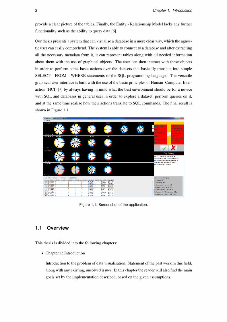
Our thesis presents a system that can visualise a database in a more clear way, which the agnos-
tic user can easily comprehend. The system is able to connect to a database and after extracting
all the necessary metadata from it, it can represent tables along with all needed information
about them with the use of graphical objects. The user can then interact with these objects
in order to perform some basic actions over the datasets that basically translate into simple
SELECT - FROM - WHERE statements of the SQL programming language. The versatile
graphical user interface is built with the use of the basic principles of Human Computer Inter-
action (HCI) [7] by always having in mind what the best environment should be for a novice
with SQL and databases in general user in order to explore a dataset, perform queries on it,
and at the same time realize how their actions translate to SQL commands. The final result is
shown in Figure 1.1.
Figure 1.1: Screenshot of the application.
1.1 Overview
This thesis is divided into the following chapters:
• Chapter 1: Introduction
Introduction to the problem of data visualisation. Statement of the past work in this field,
along with any existing, unsolved issues. In this chapter the reader will also find the main
goals set by the implementation described, based on the given assumptions.
1.2. Related Work 3
• Chapter 2: Design, tools used and system features
Description of all the tools needed for our implementation. Also, presentation of all the
basic steps taken to reach the final result and of all the features of the system.
• Chapter 3: Implementation
Thorough description of the structure of our implementation. This includes a detailed
description of all the classes in the program.
• Chapter 4: Evaluation
Presentation of scenarios and experiments for testing both the quality of the experience
delivered by the interface, as well performance and responsiveness. The framework is
tested to identify any limitations in scaling.
• Chapter 5: Conclusions and future work.
Discussion of the results, future work suggestions and conclusion.
1.2 Related Work
Database visualisation belongs to the broader category of information visualisation. In the
following few pages we are going to cover the history of information visualisation and track its
evolution through time, all the way up to our topic, the visualisation of databases. We will go
through some database visualisation techniques and also current existing implementations.
1.2.1 History of Information Visualisation
Visualisation of databases is, as already mentioned, something relatively new compared to the
much older and broader area of information visualisation [8] that can subsume tables, graphs,
maps or even possibly text; anything that attempts to visualise information in order to make it
easier to comprehend. That includes any form of representations of information that assists in
finding relationships, answering questions, or just makes it easier to draw conclusions out of it.
The recent advances in statistical computation and graphic display have provided tools capable
of performing visualisations of data unthinkable only some decades ago.
The start of visualisation of information lies about two thousand years back, when people
were making the first maps of the world and were thus trying to depict knowledge of their
surroundings in two-dimensional space to make it easier to navigate. Tables with positions of
stars and geometric diagrams started to appear as Mathematics began to flourish. The invention
4 Chapter 1. Introduction
of papyruses at the start, parchments later on and paper eventually was a very big leap forward
for visualisations, as they replaced the previously used materials (wood, cloth, stone).
The real evolution of visualisation started to occur in the 16th century, as it was then that many
techniques and instruments for measurement of physical quantities were invented. Diagrams
started to become very common in mathematical proofs; various graphics were devised to de-
pict the properties of gathered data such as their trends and distributions. Finally, in an attempt
to mix statistical thinking and cartography the now called “thematic cartography” was created.
This thematic cartography described maps that had specific attributes on them like common
geographical characteristics (mountains, rivers etc.) or more complicated characteristics (exis-
tence of certain species or spreading of diseases).
Moving on to the 17th century, here we notice a great focus on counting and visualising phys-
ical quantities. As many sciences saw significant growth (analytic geometry, physics), by the
end of this century a lot of real world data of significant interest were available, along with the
need to make sense out of them.
This need for visualisation of the gathered data was translated into a burst of evolution for
the world of visualisation in the next two centuries. Map makers were now attempting to
include even more information on maps, such as isolines and contours. Also the first attempts
at mapping economic, and medical data were made.
Carrying on to the 19th century, all of the modern statistical forms of data display were in-
vented: bar and pie charts, histograms, line graphs and others. In thematic cartography, map-
ping progressed from single maps to comprehensive atlases, depicting data on a wide variety
of topics. On the second half of the 19th century, official state statistical offices were estab-
lished throughout Europe, in recognition of the growing importance of numerical information
for commerce and transportation.
Unfortunately, the enthusiasm for innovations in visualisations did not make it into the first
half of the 20th century. There were few graphical innovations and, by the mid-1930s, the
enthusiasm had vanished. However, it was during this period that statistical graphics became
widely used. Graphical methods entered textbooks and found standard use in commerce and
science. In this period graphical methods were used, perhaps for the first time, to provide new
insights and discoveries in astronomy, physics and other sciences. For the first time a number
of practical aids to graphing were developed, and the thought of going beyond two-dimensional
graphics was put to the table.
Over the next decades, data visualisation began to rise again, especially due to the following
two facts:
• In 1962 John Tukey in his paper, “The Future of Data Analysis” [9], asked for the recog-
1.2. Related Work 5
nition of data analysis as a separate part of statistics, distinct from mathematical statis-
tics. Shortly after that he presented a wide variety of new, simple, and effective graphic
displays.
• In France, Jacques Bertin published the paper “Semiologie Graphique”[10] to organize
the visual elements of graphics according to the features and relations in data.
At the same time computer processing of data begun to offer the possibility to construct old
and new graphic forms by computer programs. High resolution graphics were developed, but
would take a while longer to enter common use. By the end of this period significant attempts
would begin that tried to combine forces of computer science research with developments in
data analysis and display and input technology (pen plotters, graphic terminals, the mouse,
etc.). These developments would provide new paradigms, languages and software packages
for expressing and implementing statistical and data graphics. In turn, they would lead to an
explosive growth in new visualisation methods and techniques. Other themes begin to emerge
such as animations of statistical processes.
Finally, as we know, from that point on the developments in data visualisation are many and
cover most of disciplines. Some of the most significant are:
• The development of a variety of highly interactive computer system.
• New methods for visualising high dimensional data (scatterplot matrix, parallel coordi-
nates plot, etc.).
• New graphical techniques for discrete and categorical data (fourfold display, sieve dia-
gram, mosaic plot, etc.).
• The application of visualisations in many existing problems and data structures.
1.2.2 Database Visualisation
All of these innovations mentioned have made it possible for visualisations to become powerful
tools for almost every discipline. In our case, in database visualisation, the major tendencies
focus around two different types of visualisations: graphs and treemaps.
1.2.2.1 Graphs
In graph visualisations, entities are represented as nodes in a graph, while references between
entities are represented as edges. The graph can be visualised in a dynamic way, meaning
that only some of the nodes are shown and the user is able to see the rest of them by gradually
6 Chapter 1. Introduction
zooming in. At the same time the shading of the nodes, the size of their names and the thickness
of the edges that connect one with the other gives to the user some information regarding the
size of the respective tables in the database and their relationships [6]. If needed, even more
ways can be used to represent special relationships or attributes (e.g. different colours in nodes
or dashed lines connecting them).
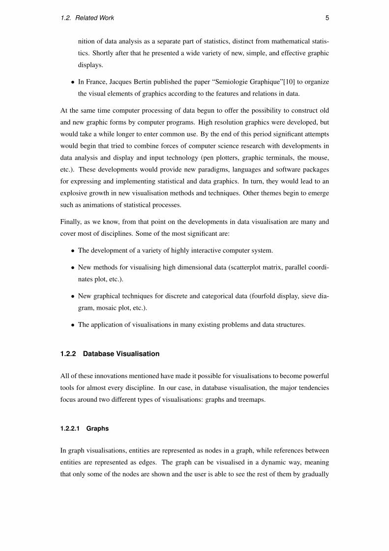
It is worth noting that graph visualisations are no good when the objects do not have any kind
of relationships between them, as in that case there would be no edges to connect the nodes.
The advantage of this representation is that it is a better fit for the human perceptual system
making the relationships between the tables easier to spot [11]. On the other hand, however,
given too many relationships the opposite happens; the outcome is too complicated for a person
to understand, as we can see in Figure 1.2 [12].
Figure 1.2: A graph with many relationships.
1.2.2.2 Treemaps
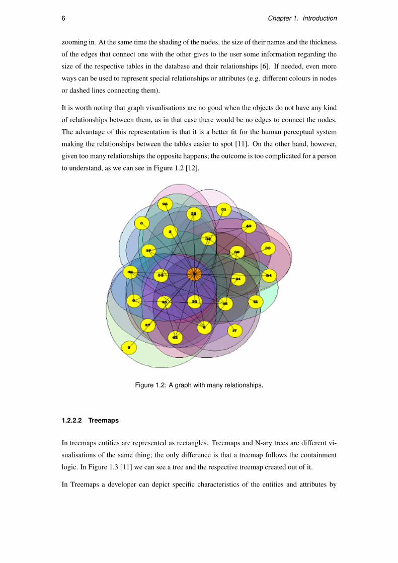
In treemaps entities are represented as rectangles. Treemaps and N-ary trees are different vi-
sualisations of the same thing; the only difference is that a treemap follows the containment
logic. In Figure 1.3 [11] we can see a tree and the respective treemap created out of it.
In Treemaps a developer can depict specific characteristics of the entities and attributes by
1.2. Related Work 7
configuring the position of the entities in the treemap, the size of the entities compared to other
entities, as well as their colour. At the same time one could potentially, following the same
logic as with graph implementations, show only the dominant entities and allow further zoom
in to reveal more information.
Figure 1.3: A treemap and its tree representation.
1.2.2.3 Visual querying in Treemaps and graphs
Whether it is a treemap or a graph, both methodologies result in a dynamic shape that the user
can interact with in order to perform visual queries. This interaction can be divided into four
different approaches:
• Clicking
The easiest form of interacting. In this case the user is able to click (left or right click
could potentially result in different actions) on certain entities in order to select them or
perform other tasks ( e.g. zoom in).
• Highlighting
Highlighting is a way of specifying subsets of a visualisation the user is interested in. It
usually takes the form of creating a rectangle around some entities.
• Dragging and dropping
The user is able to drag one entity on top of another to indicate a relationship between
them, the most common of which is issuing an equality predicate.
• Drawing Connections
An alternative to dragging and dropping elements of a visualisation is drawing connec-
tions from one entity to another. For instance, to specify a predicate between two entities
an annotated (e.g. “=”, “≤” e.t.c.) edge can be drawn between them.

8 Chapter 1. Introduction
1.2.3 Current Database Visualisation tools
Visual Query Systems (VQS) are systems that support visual representation of datasets and (in
some cases) the ability to perform visual queries. They mostly focus on the novice user and try
to provide a friendly and easy to use environment.
1.2.3.1 Query By example
Query By Example (Q.B.E) [13] is a tool developed by IBM that focuses on performing queries.
As the name of the product states it is an attempt to create a graphical user interface that
provides a new way of performing queries with the use of specific examples. The user is given
empty tables that represent the tables of the database that he/she wishes to query, and is asked
to fill the columns that he wants to see in the output with specific values or variables. A specific
example of Query By example is shown in Figure 1.4 [14]. In this query the user asks from the
system to return the content of two tables, Sailors and Reserves. As we see the column rating
of the Sailors has the value “< 4” meaning that the user is only interested in rows that have
a rating below 4. Also, both the Sailor sid column as well as the Reserves sid column have
the same value (a variable), meaning that a join needs to be performed based on that column.
Finally the sname column of the Sailors table has a “P.” which is the command for including
this column in the output (similar to SELECT clause of SQL).
Figure 1.4: Example of a ”Query By Example” query
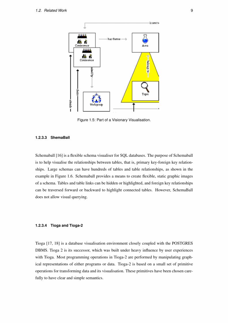
1.2.3.2 Visionary
Visionary [15] is another VQS tool that focuses on creating a realistic representation with the
help of diagrams and visual objects. The user, however, has to customize the tool prior to using
it according to the loaded database. Specifically, the user has to provide the icons that represent
each entity and relationship in the database. After this is done visual queries can be performed
by clicking on the visual objects and their relationships. These queries are then translated into
SQL and executed. In this way the user does not need to have any prior knowledge of SQL.
However, the setup process limits the project. In Figure 1.5 [15] a screenshot of visionary
visualising a database about conferences is shown.
1.2. Related Work 9
Figure 1.5: Part of a Visionary Visualisation.
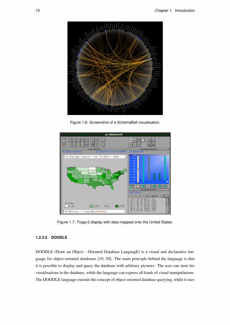
1.2.3.3 ShemaBall
Schemaball [16] is a flexible schema visualiser for SQL databases. The purpose of Schemaball
is to help visualise the relationships between tables, that is, primary key-foreign key relation-
ships. Large schemas can have hundreds of tables and table relationships, as shown in the
example in Figure 1.6. Schemaball provides a means to create flexible, static graphic images
of a schema. Tables and table links can be hidden or highlighted, and foreign key relationships
can be traversed forward or backward to highlight connected tables. However, SchemaBall
does not allow visual querying.
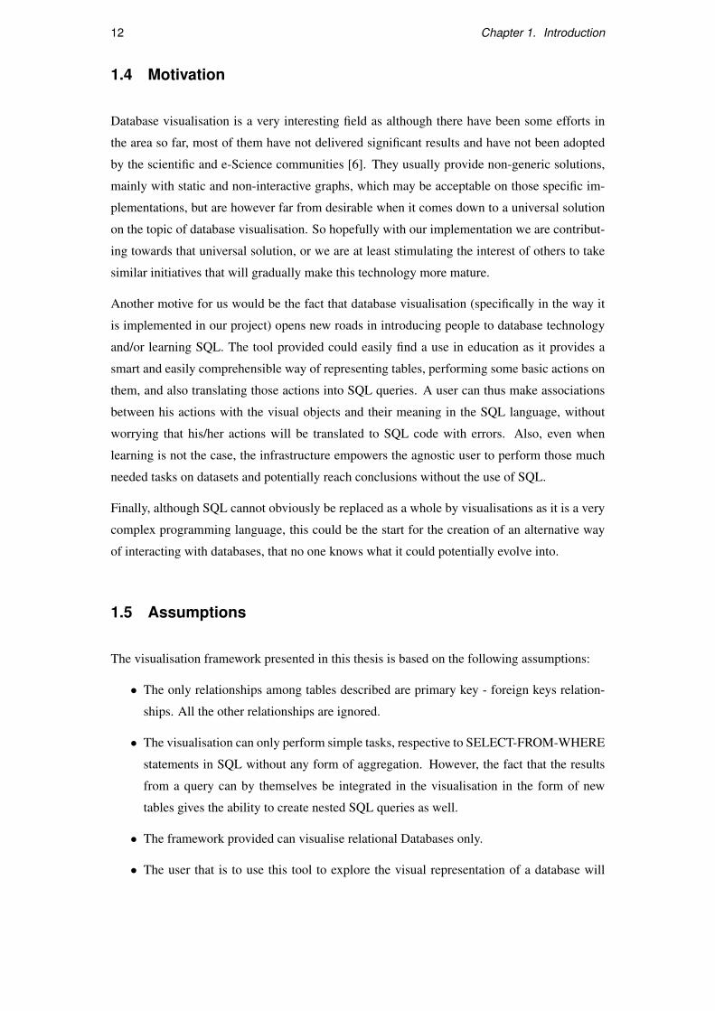
1.2.3.4 Tioga and Tioga-2
Tioga [17, 18] is a database visualisation environment closely coupled with the POSTGRES
DBMS. Tioga 2 is its successor, which was built under heavy influence by user experiences
with Tioga. Most programming operations in Tioga-2 are performed by manipulating graph-
ical representations of either programs or data. Tioga-2 is based on a small set of primitive
operations for transforming data and its visualisation. These primitives have been chosen care-
fully to have clear and simple semantics.
10 Chapter 1. Introduction
Figure 1.6: Screenshot of a SchemaBall visualisation.
Figure 1.7: Tioga-2 display with data mapped onto the United States.
1.2.3.5 DOODLE
DOODLE (Draw an Object - Oriented Database LanguagE) is a visual and declarative lan-
guage for object-oriented databases [19, 20]. The main principle behind the language is that
it is possible to display and query the database with arbitrary pictures. The user can store his
visualisations in the database, while the language can express all kinds of visual manipulations.
The DOODLE language extends the concept of object-oriented database querying, while it uses

1.3. Goals 11
the technology of deductive query languages for object-oriented databases as its foundation.
1.2.3.6 Delaunay
Delaunay [21] is an interactive system for the declarative querying and displaying of object-
oriented databases. It is implemented using Java and supports visualisations of object-oriented
databases specified by the user with a visual constraint-based query language. The highlights
of this approach are the expressiveness of the visual query language, the efficiency of the query
engine and the overall flexibility and extensibility of the framework. Delaunay is based on the
visual database query language DOODLE. Users can arrange graphical objects and graphical
constraints to form a “picture” that specifies how to visualise objects belonging to a class.
1.3 Goals
The main goal of this project is to create a solid infrastructure that can visualise the main
characteristics of a relational database regardless of its schema or size using graphics in two
- dimensional space. The user will be able to connect to the database he chooses, see its
visualisation and also interact with it by performing visual queries that have the same effects
as simple SELECT - FROM - WHERE SQL queries. This implementation focuses on novice
users and allows them to gain some form of control over the data without any need of knowing
a programming language. All in all, the main goals are the following:
• Create a tool that can be used on any database (given the current assumptions as they are
described in Section 1.5 without any constraints regarding the databases schema or size.
• Make this tool designed for use by novice databases users that are still learning the basic
principles of database and SQL programming. Potentially, also provide an alternative to
the usual process of learning about Databases or SQL.
• Provide a smooth user experience by making a multi-threaded infrastructure so that the
user interface never freezes when background tasks are performed. Also use prefetching
of data from the database when possible in an attempt to minimize the time that the users
wait for results.
• Provide the ability of accessing the infrastructure through the web.
• Create an all-around pleasant environment for the user to work in by respecting the main
principles of Human Computer Interaction [7].
12 Chapter 1. Introduction
1.4 Motivation
Database visualisation is a very interesting field as although there have been some efforts in
the area so far, most of them have not delivered significant results and have not been adopted
by the scientific and e-Science communities [6]. They usually provide non-generic solutions,
mainly with static and non-interactive graphs, which may be acceptable on those specific im-
plementations, but are however far from desirable when it comes down to a universal solution
on the topic of database visualisation. So hopefully with our implementation we are contribut-
ing towards that universal solution, or we are at least stimulating the interest of others to take
similar initiatives that will gradually make this technology more mature.
Another motive for us would be the fact that database visualisation (specifically in the way it
is implemented in our project) opens new roads in introducing people to database technology
and/or learning SQL. The tool provided could easily find a use in education as it provides a
smart and easily comprehensible way of representing tables, performing some basic actions on
them, and also translating those actions into SQL queries. A user can thus make associations
between his actions with the visual objects and their meaning in the SQL language, without
worrying that his/her actions will be translated to SQL code with errors. Also, even when
learning is not the case, the infrastructure empowers the agnostic user to perform those much
needed tasks on datasets and potentially reach conclusions without the use of SQL.
Finally, although SQL cannot obviously be replaced as a whole by visualisations as it is a very
complex programming language, this could be the start for the creation of an alternative way
of interacting with databases, that no one knows what it could potentially evolve into.
1.5 Assumptions
The visualisation framework presented in this thesis is based on the following assumptions:
• The only relationships among tables described are primary key - foreign keys relation-
ships. All the other relationships are ignored.
• The visualisation can only perform simple tasks, respective to SELECT-FROM-WHERE
statements in SQL without any form of aggregation. However, the fact that the results
from a query can by themselves be integrated in the visualisation in the form of new
tables gives the ability to create nested SQL queries as well.
• The framework provided can visualise relational Databases only.
• The user that is to use this tool to explore the visual representation of a database will

1.5. Assumptions 13
need to go either through a manual (or parts of this thesis), or he/she will need some kind
of demonstration. All in all, this tool is very easy to use, but is not self-explanatory for
the agnostic user.
• Although technically able to support any database with any number of tables, with them
containing any number of columns, with or without any dependencies among them, this
visualisation lacks some tools to help the user navigate easily in vast databases. Also
when the number of columns in tables increases by a lot, their names do not appear
as this is impossible, making it thus harder (but not impossible) to recognise specific
columns. Due to these issues the assumption was made that this tool is going to be used
for smaller databases, where its full potential shines.


Chapter 2
System Design and features
The design of this tool started by gathering all the requirements for it. That, in itself, gave us
an idea of what the tool would be able to do, what it would not do, as well as a rough idea of
how it would perform all the needed actions. Due to the implementation relying heavily on a
graphical user interface, it was decided that a few mock-ups had to be created first so that the
main issues around the interface were solved before the actual coding started. This saved us
some time from having to alter the code multiple times before deciding on the exact structure
of the interface.
The strategy that was followed during the implementation was to start with a graphical user
interface without any functionality, and slowly add features to it, thus gradually transforming it
into our visualisation tool. During this process refactoring of the code was performed several
times, to make sure that the tool would remain flexible and fast.
In general the main steps during the creation of the tool were the following:
• Achieve connection with the DBMS.
• Extract all the needed metadata from the DBMS.
• Use all the extracted metadata to create structures that could be visualised.
• Add user interaction to the visualisation (the program would now respond to mouse
movement and clicking on objects).
• Transform this user interaction into SQL queries and attempt to pose these queries against
the database.
• Add join functionality into the program.
• Make some changes so that it can be run by the internet as a web application.
15
16 Chapter 2. System Design and features
Obviously, by creating one part of the program at a time and gradually adding features on it,
we managed to come up with many more ideas to make this tool more responsive and easy to
use. These ideas were implemented, tested and integrated into the system. Also, during the
evaluation of the visualisation tool, the users that tested the program had some very good and
innovative ideas that could give even greater functionality to the program. Although it was not
mandatory to implement these ideas as our tool was quite complete as it was, it was decided to
implement them anyway. This lead the program to the form it has now.
2.1 Tools and libraries used
A plethora of tools was used so that the best possible results could be achieved. The coding of
the project was performed with the help of the NetBeans IDE, while the Database Management
System used is Microsoft SQL Server. Apart from these tools, many other smaller tools were
used and are described in the following pages.
2.1.1 Processing
Processing [22] is an open source programming language and environment for people who want
to create images, animations, and interactions. Processing, although it was initially developed
to teach fundamentals of computer programming within a visual context, evolved into a tool
for generating finished professional work.
This tool was chosen to help with the visualisation of the databases as it can be very easily
integrated with JAVA, and can thus provide a sophisticated framework for graph modelling
and layout. Processing provides an easy way to handle keyboard and mouse events, and at
the same time it implements many functions and features for the developer to start with. The
user has complete control over what is drawn, where it is drawn and how it is drawn. As an
example, anti-aliasing is just one function away (smooth function). However, there are many
more advantages as there are libraries in processing that can make processing support:
• Viewing and creating movies
• OpenGL accelerated sketches
• Network compliance
• Sound integration
• Pdf support
• XML support

2.1. Tools and libraries used 17
Finally, Processing is widely used, as thousands of people use it to create graphics, even at
professional level. Also, there are many tutorials and books for it, making it very easy for
someone to get to know the platform.
2.1.2 Microsoft SQL Server
Microsofts DBMS was chosen for this implementation. There are a few very good DBMSs in
the market, but this one was chosen as the writer already had some experience with setting it
up, and at the same time a trial version of six months was available at the time of writing. The
version used is Microsoft SQL server 2008 R2.
2.1.3 JDBC
Java DataBase Connectivity, or JDBC is a library that, as stated by the name, allows the con-
nection of a Java application with a database; This JDBC API defines how a client may access
a database. It is oriented towards relational databases and provides methods for querying and
updating data in a database [23]. The great advantage of JDBC is that it is cross-platform,
meaning that the API it provides can work on any Database Management System. Figure 2.1
shows the basic structure of the JDBC package. In a few words, this package includes functions
that are implemented in many different ways, one for each database management system that
is supported. When a connection is initiated, the user defines on what DBMS he/she is trying
to connect to, making the JDBC driver manager able to pick the correct implementation of the
functions that user will call later.
2.1.4 Xampp
XAMPP [24] is an easy to install, open source Apache distribution containing MySQL, PHP
and Perl. The name comes from the words X (cross, meaning cross-platform) A (Apache
HTTPS Server) M (MySQL) P (PHP) P (Perl)
It was chosen for the implementation of the web server, in order to make our application run
on the web as an Applet. The reason why it was chosen is because it is very easy to install and
the writer already had some previous experience with this tool. Indeed, it only took us about
twenty minutes to have the web server up and running.

18 Chapter 2. System Design and features
Figure 2.1: Structure of the JDBC drivers.
2.1.5 JarSigner
This tool is built-in in the JDK (Java Development Kit). What it does is that it generates
signatures for Java Archive files (JAR files) [25]. This tool was needed as running an applet on
a web server imposes specific security constraints on the actions allowed to the applet, unless
it is signed. For example, unless signed the applet is not allowed to connect to a database.
2.1.6 NetBeans IDE
The NetBeans IDE was chosen for the writing of this Java Application. The version used it
version 6.9.1. This choice was made only because the write has a lot of experience with this
tool. At the same time it contains another very useful tool that was used, the NetBeans Profiler,
which provides specific memory allocation and performance monitoring utility. More on the
NetBeans Profiler can be found in chapter 4.
2.2 System features
In a few words, this application is able to connect to a database, retrieve some information from
it and visualise it. After that the application provides a way to perform visual queries, which are
then translated to simple “SELECT - FROM - WHERE” SQL queries and are posed against the
database. Finally the results of these visual queries appear on the graphical user interface so that
2.2. System features 19
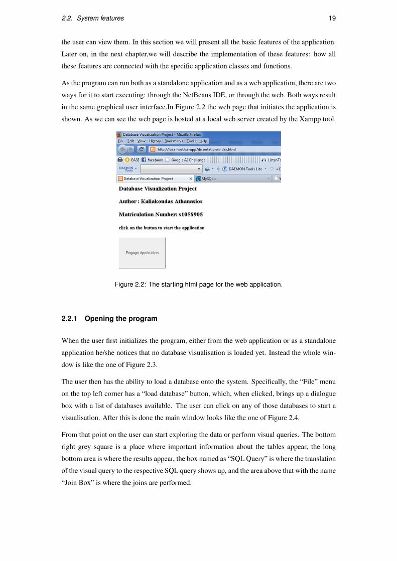
the user can view them. In this section we will present all the basic features of the application.
Later on, in the next chapter,we will describe the implementation of these features: how all
these features are connected with the specific application classes and functions.
As the program can run both as a standalone application and as a web application, there are two
ways for it to start executing: through the NetBeans IDE, or through the web. Both ways result
in the same graphical user interface.In Figure 2.2 the web page that initiates the application is
shown. As we can see the web page is hosted at a local web server created by the Xampp tool.
Figure 2.2: The starting html page for the web application.
2.2.1 Opening the program
When the user first initializes the program, either from the web application or as a standalone
application he/she notices that no database visualisation is loaded yet. Instead the whole win-
dow is like the one of Figure 2.3.
The user then has the ability to load a database onto the system. Specifically, the “File” menu
on the top left corner has a “load database” button, which, when clicked, brings up a dialogue
box with a list of databases available. The user can click on any of those databases to start a
visualisation. After this is done the main window looks like the one of Figure 2.4.
From that point on the user can start exploring the data or perform visual queries. The bottom
right grey square is a place where important information about the tables appear, the long
bottom area is where the results appear, the box named as “SQL Query” is where the translation
of the visual query to the respective SQL query shows up, and the area above that with the name
“Join Box” is where the joins are performed.

20 Chapter 2. System Design and features
Figure 2.3: The initial application window.
The user from this point can start clicking on the visualisation to interact with it. By performing
these actions the user can go into different visualisation “modes”. In general, the implemen-
tation supports three different modes: the normal mode, the zoom mode and the relationship
mode. The normal mode is the one that the user sees when he/she starts a visualisation. From
this mode the user can switch to the other two modes, the relationship mode and the zoom
mode. The relationship mode gives the user the ability to just view the tables related to a spe-
cific table (in terms of primary key/foreign key relationships), while the zoom mode allows the
user to see more information about a specific table, and also perform the visual query part of
the implementation. As mentioned earlier, after recommendations coming from the users, it
was decided to allow the creation of joins from the relationship mode as well, as at that point
the user would see all the relationships among tables anyway, so it would be easier to choose
the right columns for the joins.
2.2.2 Relationship Mode
The relationship mode is enabled when the user right clicks on a specific table. In this way the
user states that he wants to see all the primary key/foreign key relationships of this table with
the rest of the tables in the database. When this happens, all the tables that are not related to
the table that was clicked disappear. At the same time, the tables that are related have their
trivial columns (the columns that have nothing to do with the specific primary key/foreign key
relationship) faded, while the rest of the columns gain specific numbers so that it is easy to
match a primary key from one table with a foreign key from another, as shown in Figure 2.5.
At the same time while the user sees all these relationships, he is allowed to right click on

2.2. System features 21
Figure 2.4: The application with a loaded visualisation.
columns in order to perform joins as we will see later on.
Figure 2.5: Screenshot of the application while in relationship mode.
2.2.3 Zoom Mode
The zoom mode is enabled when the user left clicks anywhere on a sketch. In this way the user
states that he wants to have a better look at that specific sketch. When this happens, the height
of the particular sketch gets doubled, and it comes in the centre of the screen. At the same time
some additional attributes appear: the column names, and the primary key column which now
has its name painted in yellow. All the columns gradually fade out with an animation-like drop
of transparency, as the system is now ready for the user to start performing the visual query;
the user can either left click on any column to include it in his query, or he can right click on it
22 Chapter 2. System Design and features
in order to include it in a join.
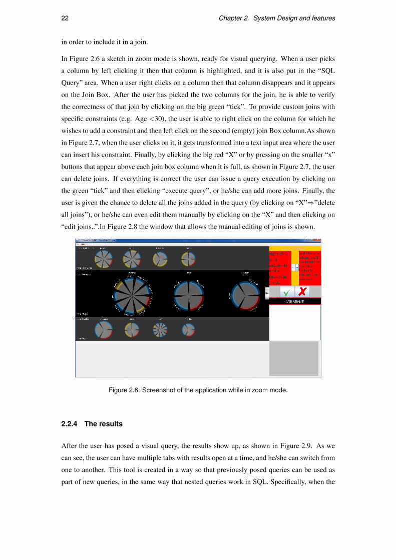
In Figure 2.6 a sketch in zoom mode is shown, ready for visual querying. When a user picks
a column by left clicking it then that column is highlighted, and it is also put in the “SQL
Query” area. When a user right clicks on a column then that column disappears and it appears
on the Join Box. After the user has picked the two columns for the join, he is able to verify
the correctness of that join by clicking on the big green “tick”. To provide custom joins with
specific constraints (e.g. Age <30), the user is able to right click on the column for which he
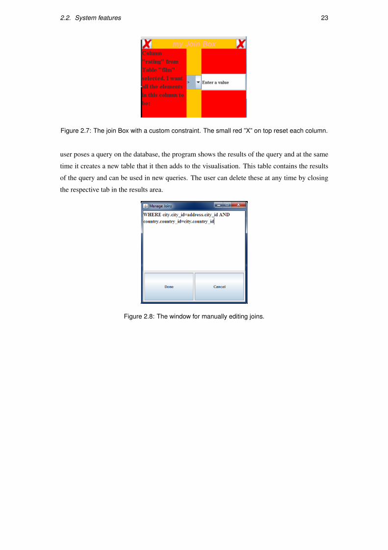
wishes to add a constraint and then left click on the second (empty) join Box column.As shown
in Figure 2.7, when the user clicks on it, it gets transformed into a text input area where the user
can insert his constraint. Finally, by clicking the big red “X” or by pressing on the smaller “x”
buttons that appear above each join box column when it is full, as shown in Figure 2.7, the user
can delete joins. If everything is correct the user can issue a query execution by clicking on
the green “tick” and then clicking “execute query”, or he/she can add more joins. Finally, the
user is given the chance to delete all the joins added in the query (by clicking on “X”⇒”delete
all joins”), or he/she can even edit them manually by clicking on the “X” and then clicking on
“edit joins..”.In Figure 2.8 the window that allows the manual editing of joins is shown.
Figure 2.6: Screenshot of the application while in zoom mode.
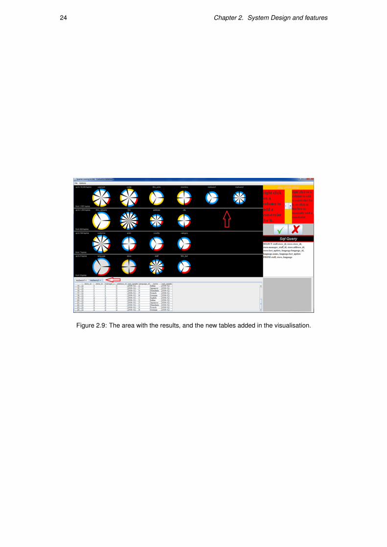
2.2.4 The results
After the user has posed a visual query, the results show up, as shown in Figure 2.9. As we
can see, the user can have multiple tabs with results open at a time, and he/she can switch from
one to another. This tool is created in a way so that previously posed queries can be used as
part of new queries, in the same way that nested queries work in SQL. Specifically, when the
2.2. System features 23
Figure 2.7: The join Box with a custom constraint. The small red ”X” on top reset each column.
user poses a query on the database, the program shows the results of the query and at the same
time it creates a new table that it then adds to the visualisation. This table contains the results
of the query and can be used in new queries. The user can delete these at any time by closing
the respective tab in the results area.
Figure 2.8: The window for manually editing joins.
24 Chapter 2. System Design and features
Figure 2.9: The area with the results, and the new tables added in the visualisation.
Chapter 3
Implementation
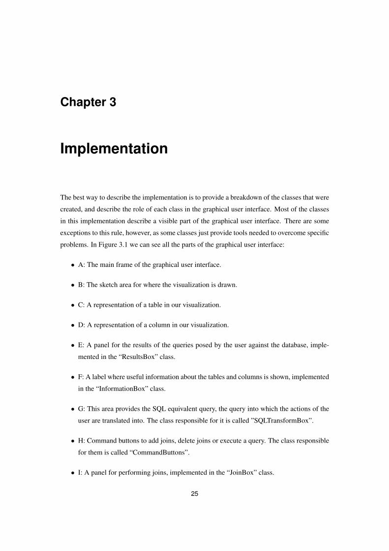
The best way to describe the implementation is to provide a breakdown of the classes that were
created, and describe the role of each class in the graphical user interface. Most of the classes
in this implementation describe a visible part of the graphical user interface. There are some
exceptions to this rule, however, as some classes just provide tools needed to overcome specific
problems. In Figure 3.1 we can see all the parts of the graphical user interface:
• A: The main frame of the graphical user interface.
• B: The sketch area for where the visualization is drawn.
• C: A representation of a table in our visualization.
• D: A representation of a column in our visualization.
• E: A panel for the results of the queries posed by the user against the database, imple-
mented in the “ResultsBox” class.
• F: A label where useful information about the tables and columns is shown, implemented
in the “InformationBox” class.
• G: This area provides the SQL equivalent query, the query into which the actions of the
user are translated into. The class responsible for it is called ”SQLTransformBox”.
• H: Command buttons to add joins, delete joins or execute a query. The class responsible
for them is called “CommandButtons”.
• I: A panel for performing joins, implemented in the “JoinBox” class.
25

26 Chapter 3. Implementation
3.1 Database Connection
For the implementation to work, a database connection is obligatory. The system must be able
to connect to a database and extract all the necessary metadata (names of columns and tables,
cardinalities primary keys, foreign keys etc.) of it in order to have something to visualize.
As such, the first step taken in the construction of this software, before implementing any
parts of the graphical user interface was the establishment of a connection with a database,
and the extraction of all the necessary data from it. The JDBC library that has been used in
this implementation gives an easy to use, cross-platform environment both for connecting to a
database, as well as for extracting all the necessary metadata.
Figure 3.1: A breakdown of the graphical objects taking part in the implementation.
3.1.1 The connection
The connection is performed by the Database class. This class is responsible for:
• Creating a connection to the database
• Extracting metadata
• Constructing table objects
• Creating an index based on which the table objects are allocated to the four main sketch
areas.
3.1. Database Connection 27
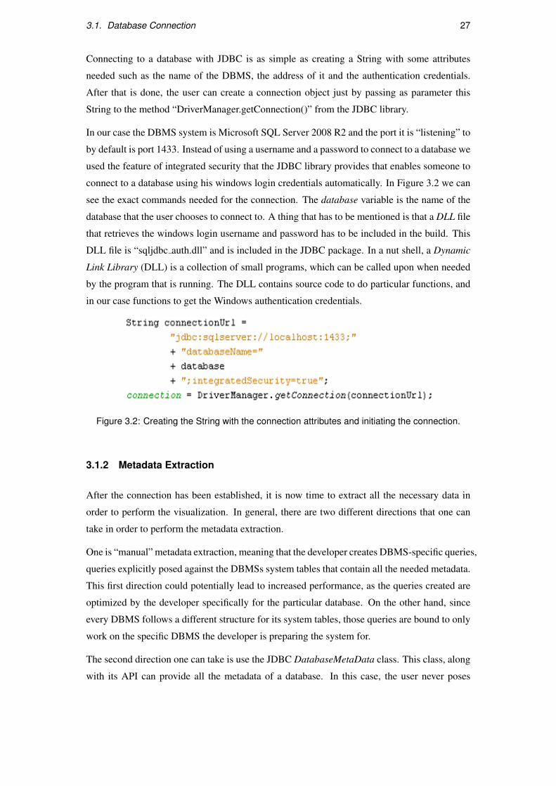
Connecting to a database with JDBC is as simple as creating a String with some attributes
needed such as the name of the DBMS, the address of it and the authentication credentials.
After that is done, the user can create a connection object just by passing as parameter this
String to the method “DriverManager.getConnection()” from the JDBC library.
In our case the DBMS system is Microsoft SQL Server 2008 R2 and the port it is “listening” to
by default is port 1433. Instead of using a username and a password to connect to a database we
used the feature of integrated security that the JDBC library provides that enables someone to
connect to a database using his windows login credentials automatically. In Figure 3.2 we can
see the exact commands needed for the connection. The database variable is the name of the
database that the user chooses to connect to. A thing that has to be mentioned is that a DLL file
that retrieves the windows login username and password has to be included in the build. This
DLL file is “sqljdbc auth.dll” and is included in the JDBC package. In a nut shell, a Dynamic
Link Library (DLL) is a collection of small programs, which can be called upon when needed
by the program that is running. The DLL contains source code to do particular functions, and
in our case functions to get the Windows authentication credentials.
Figure 3.2: Creating the String with the connection attributes and initiating the connection.
3.1.2 Metadata Extraction
After the connection has been established, it is now time to extract all the necessary data in
order to perform the visualization. In general, there are two different directions that one can
take in order to perform the metadata extraction.
One is “manual” metadata extraction, meaning that the developer creates DBMS-specific queries,
queries explicitly posed against the DBMSs system tables that contain all the needed metadata.
This first direction could potentially lead to increased performance, as the queries created are
optimized by the developer specifically for the particular database. On the other hand, since
every DBMS follows a different structure for its system tables, those queries are bound to only
work on the specific DBMS the developer is preparing the system for.
The second direction one can take is use the JDBC DatabaseMetaData class. This class, along
with its API can provide all the metadata of a database. In this case, the user never poses
28 Chapter 3. Implementation
queries on his/her own, but just selects specific functions from the DatabaseMetaData class
that return the metadata. Obviously, on their implementation, these functions pose queries on
the database System tables (potentially even the same queries that the developer would write).
This abstract way of retrieving the metadata makes it possible for the database connection to
be cross-platform, meaning that no matter what DBMS is used, it is up to the JDBC library
and the implementation of the functions it carries to pose the correct queries for the respective
database.
In our implementation both ways were implemented, and the second one, apart from being
cross platform, was found to be faster than the first one (possibly due to the fact that the devel-
opers of the JDBC library were able to write more efficient queries), and was finally chosen to
be included in our project. The alternative, however, first direction is included in Appendix A.
Carrying on to the actual implementation, the DatabaseMetaData class from the JDBC library
was used. This object is initialized with the use of the already established connection, and
provides all the information we are going to need.
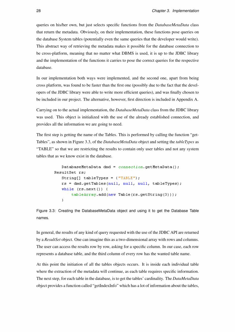
The first step is getting the name of the Tables. This is performed by calling the function “get-
Tables”, as shown in Figure 3.3, of the DatabaseMetaData object and setting the tableTypes as
“TABLE” so that we are restricting the results to contain only user tables and not any system
tables that as we know exist in the database.
Figure 3.3: Creating the DatabaseMetaData object and using it to get the Database Table
names.
In general, the results of any kind of query requested with the use of the JDBC API are returned
by a ResultSet object. One can imagine this as a two-dimensional array with rows and columns.
The user can access the results row by row, asking for a specific column. In our case, each row
represents a database table, and the third column of every row has the wanted table name.
At this point the initiation of all the tables objects occurs. It is inside each individual table
where the extraction of the metadata will continue, as each table requires specific information.
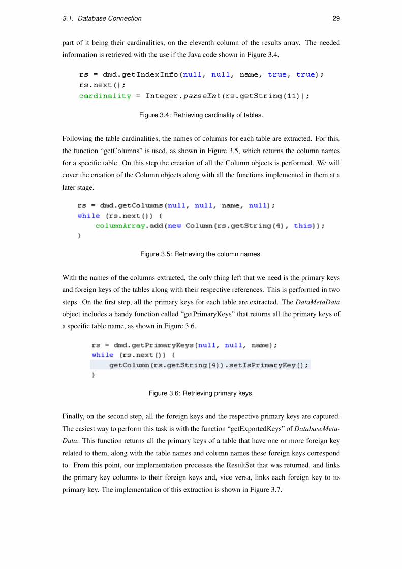
The next step, for each table in the database, is to get the tables’ cardinality. The DataMetaData
object provides a function called “getIndexInfo” which has a lot of information about the tables,
3.1. Database Connection 29
part of it being their cardinalities, on the eleventh column of the results array. The needed
information is retrieved with the use if the Java code shown in Figure 3.4.
Figure 3.4: Retrieving cardinality of tables.
Following the table cardinalities, the names of columns for each table are extracted. For this,
the function “getColumns” is used, as shown in Figure 3.5, which returns the column names
for a specific table. On this step the creation of all the Column objects is performed. We will
cover the creation of the Column objects along with all the functions implemented in them at a
later stage.
Figure 3.5: Retrieving the column names.
With the names of the columns extracted, the only thing left that we need is the primary keys
and foreign keys of the tables along with their respective references. This is performed in two
steps. On the first step, all the primary keys for each table are extracted. The DataMetaData
object includes a handy function called “getPrimaryKeys” that returns all the primary keys of
a specific table name, as shown in Figure 3.6.
Figure 3.6: Retrieving primary keys.
Finally, on the second step, all the foreign keys and the respective primary keys are captured.
The easiest way to perform this task is with the function “getExportedKeys” of DatabaseMeta-
Data. This function returns all the primary keys of a table that have one or more foreign key
related to them, along with the table names and column names these foreign keys correspond
to. From this point, our implementation processes the ResultSet that was returned, and links
the primary key columns to their foreign keys and, vice versa, links each foreign key to its
primary key. The implementation of this extraction is shown in Figure 3.7.

30 Chapter 3. Implementation
Figure 3.7: Linking primary keys to their foreign keys and vice versa.
3.2 Allocating the tables to sketches
After the extraction of the information from the database, the visualization takes place. Now
that we know exactly how many tables we have, their cardinalities, and the primary key/foreign
key relationships between them we can draw them. As we see in Figure 3.8, the visualization
area consists of four main empty spaces in black colour, divided by white lines.
Figure 3.8: The four sketches that comprise the visualisation area without any tables in them.
3.3. The Graphical User Interface 31
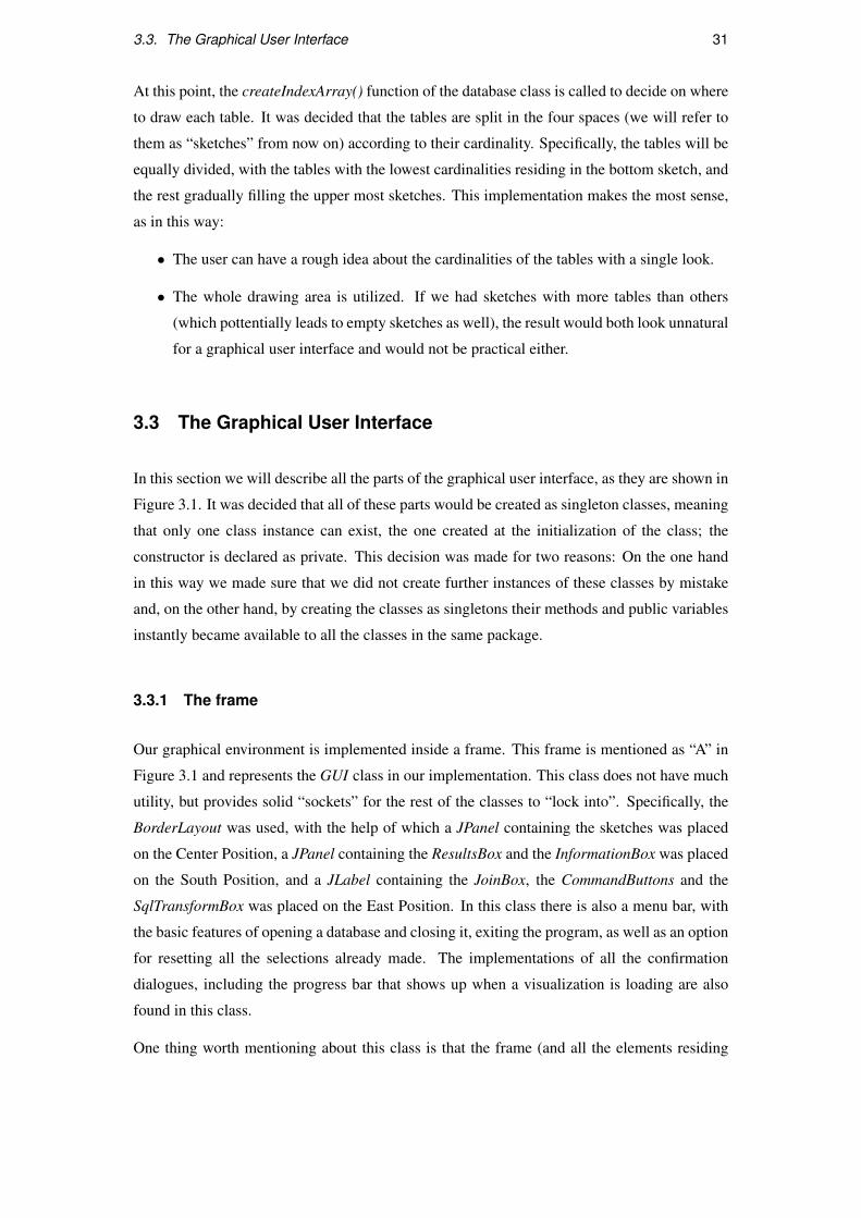
At this point, the createIndexArray() function of the database class is called to decide on where
to draw each table. It was decided that the tables are split in the four spaces (we will refer to
them as “sketches” from now on) according to their cardinality. Specifically, the tables will be
equally divided, with the tables with the lowest cardinalities residing in the bottom sketch, and
the rest gradually filling the upper most sketches. This implementation makes the most sense,
as in this way:
• The user can have a rough idea about the cardinalities of the tables with a single look.
• The whole drawing area is utilized. If we had sketches with more tables than others
(which pottentially leads to empty sketches as well), the result would both look unnatural
for a graphical user interface and would not be practical either.
3.3 The Graphical User Interface
In this section we will describe all the parts of the graphical user interface, as they are shown in
Figure 3.1. It was decided that all of these parts would be created as singleton classes, meaning
that only one class instance can exist, the one created at the initialization of the class; the
constructor is declared as private. This decision was made for two reasons: On the one hand
in this way we made sure that we did not create further instances of these classes by mistake
and, on the other hand, by creating the classes as singletons their methods and public variables
instantly became available to all the classes in the same package.
3.3.1 The frame
Our graphical environment is implemented inside a frame. This frame is mentioned as “A” in
Figure 3.1 and represents the GUI class in our implementation. This class does not have much
utility, but provides solid “sockets” for the rest of the classes to “lock into”. Specifically, the
BorderLayout was used, with the help of which a JPanel containing the sketches was placed
on the Center Position, a JPanel containing the ResultsBox and the InformationBox was placed
on the South Position, and a JLabel containing the JoinBox, the CommandButtons and the
SqlTransformBox was placed on the East Position. In this class there is also a menu bar, with
the basic features of opening a database and closing it, exiting the program, as well as an option
for resetting all the selections already made. The implementations of all the confirmation
dialogues, including the progress bar that shows up when a visualization is loading are also
found in this class.
One thing worth mentioning about this class is that the frame (and all the elements residing

32 Chapter 3. Implementation
in it) is built so that it can be displayed in any screen resolution without any problems. Our
implementation was created with a resolution of 1600x900, and the screenshot from Figure 3.1
is taken in that resolution. However, the screenshot in Figure 3.9 is taken at a 1024x768 screen
resolution, and as we can see they are almost identical.
To have such a result, wherever it was needed to put dimensions (e.g. Panels sizes, Font sizes),
instead of giving absolute numbers, we gave percentages of the screens’ width and height.
Also, we made sure that all the images used in the implementation were dynamically rescaled
accordingly, as shown in the code snippet in Figure 3.10.
Figure 3.9: Screenshot of the application while running at 1024 x 768 screen resolution.
Figure 3.10: The scale function dynamically rescales an image according to the current Screen
Resolution.

3.3. The Graphical User Interface 33
3.3.2 The Sketches
The sketches have the letter “B” in Figure 3.1 and are materialized in the Sketch Class. It was
decided that instead of creating one large sketch that would contain the whole visualization,
four individual sketches would be created; one representing each section of the visualization.
Those sketches can of course “talk” to each other in order to perform more advanced tasks.
As these four sections of the visualization had to behave in the same way our approach seems
superior to creating a single bigger sketch that had a lot of code replication inside it.
The Sketch class extends the PApplet class, which is a class from the Processing Library. In
this way all the handy tools of the Processing API can be used. The basic idea behind the
PApplet is that it has a setup() function that is used only when this object is starting up, and
a draw() function that is called as many times per second as the frame rate is set to. In our
implementation the frame rate has been set to twenty frames per second.
In the setup() function some instantiation of objects occurs, along with the registration of each
sketch for listening to mouse events and the loading of all needed images. As a side note, the
Processing API provides a resize() function that takes care of resizing images so that images
inside the sketches (in our case the arrows in each sketch) can be displayed correctly on any
screen resolution.
The draw() function is the “heart” of the visualization. The Sketch.draw() function is the small-
est out of the three draw functions in total (one in the Sketch class, one in the Table class and one
in the Column class). It is responsible for printing out the white line separating the sketches, the
background (with specific transparencies when needed), printing the range of the cardinalities
on the top left and bottom left corner, print the navigational arrows as well as process clicks on
them to scroll the visualization in the desired direction. These arrows are there to make sure
that the user can see all the tables of the visualization, in case there are too many of them to fit.
However, they are not static but dynamic, meaning that they do not appear when there are too
few Tables in a Sketch, or when the scrolling limits are reached. Figure 3.11 depicts a sketch,
along with the navigational arrows. We notice that the right navigational arrow is appearing
while the left one is not. This is because there are more tables to the right but there are no
tables to the left as the left most table is already in the visual range.
Figure 3.11: A sketch with the right navigational arrow appearing.
The draw() function in the Sketch class has one more role. It invokes the draw() function of

34 Chapter 3. Implementation
each Table so that it can be drawn. Prior to performing this action, the sketch class has to decide
which tables are going to get drawn and where in the sketch they are going to get drawn. Each
sketch already has some tables allocated to it by the index array that was created previously
by the database class. However, these allocated tables are not printed always. Specifically,
when the visualization is running on relationship mode it only draws the tables that have some
primary key/foreign key relationship with the clicked table. After the to-be printed tables
have been determined, the position of each table has to be calculated. The processing library
provides two very useful functions for this, pushMatrix() and popMatrix().
In general, a Processing sketch works like a piece of graph paper. When one wants to draw
something, he/she has to specify its coordinates on the graph. For example when drawing
a rectangle one has to include four parameters: its starting position x-coordinate, its starting
position y-coordinate and its width and height. If then the rectangle needs to be moved 60
units right and 80 units down, one can just change the coordinates by adding to the x and y
starting point, and the rectangle will appear in a different place. Processing, however gives an
alternative to that; it allows the user to move the graph paper instead. Moving the graph paper
(or “coordinate system”), results in the same visual result. Moving the coordinate system is
called translation. pushMatrix() is a built-in function that saves the current position of the
coordinate system. Then, a translate(x, y) call will move the coordinate system x units right
and y units down. Then the drawing can take place, and finally the popMatrix() restores the
coordinate system to the way it was before the translation was performed.
This is very useful for drawing as it simplifies things. The way the pushMatrix() and pop-
Matrix() functions are used in our implementation is shown in Figure 3.12. As we notice, for
each table the pushMatrix() function is called, the specific location of the table is calculated,
the translation occurs and then the Table.draw() function is called. Finally the popMatrix()
function is called to restore the coordinate system back to its previous position.
Figure 3.12: Code snippet with part of the Sketch.draw() function.
Another important function in the Sketch class is mouseEvent(). MouseEvent() is the function
that handles all the user actions, for all the three classes that provide visualization in our tool
(Sketches, Tables and Columns). In a few lines, this function continuously tracks on which
3.3. The Graphical User Interface 35
“mode” the application is in (normal mode, relationship mode or zoom mode) and what actions
the user is performing at the moment (dragging his/her mouse over the visualizations, left
clicking or right clicking). As shown in Figure 3.13 the main options are:
• Track mouse movement and update the InformationBox accordingly. When the mouse
is on top of a column, the specific information of that column is printed on the Informa-
tionBox to inform the user. As a side note, clicking on arrows is handled by the draw()
function instead of this one, as in this way the scrolling of the sketches is more smooth.
• Track left clicking of the mouse and toggle the zoom mode accordingly or select columns
for a visual query. Specifically, when the application is in normal mode or relationship
mode, a click anywhere on the sketches switches it to zoom mode. If it is on zoom mode
already, then a left click anywhere except for the tables brings it back to normal mode. If
the tables are clicked while in zoom mode, then the specific column clicked is included
in the “SELECT” clause of the respective SQL query, while if it is clicked again it is
excluded.
• Track right clicking of the mouse and toggle relationship mode accordingly, or select
columns that are added in Joins. Specifically, when the application is in normal mode,
a click on a table switches the application to relationship mode for that table. From that
point on the user has two options: he/she can right click again on a Column to include it
in a Join, or he/she can right click anywhere else to go back to normal mode.
These are the basic functions of the Table class. Obviously, there are many more functions that
are either trivial (such as the “set” or “get” functions to get or set values of specific variables
that are declared as “private” in the class), or not that trivial (such as functions that enable the
different modes of the program.). However, due to the large number of them (approximately
30), it is out of the scope of this thesis to describe them all.
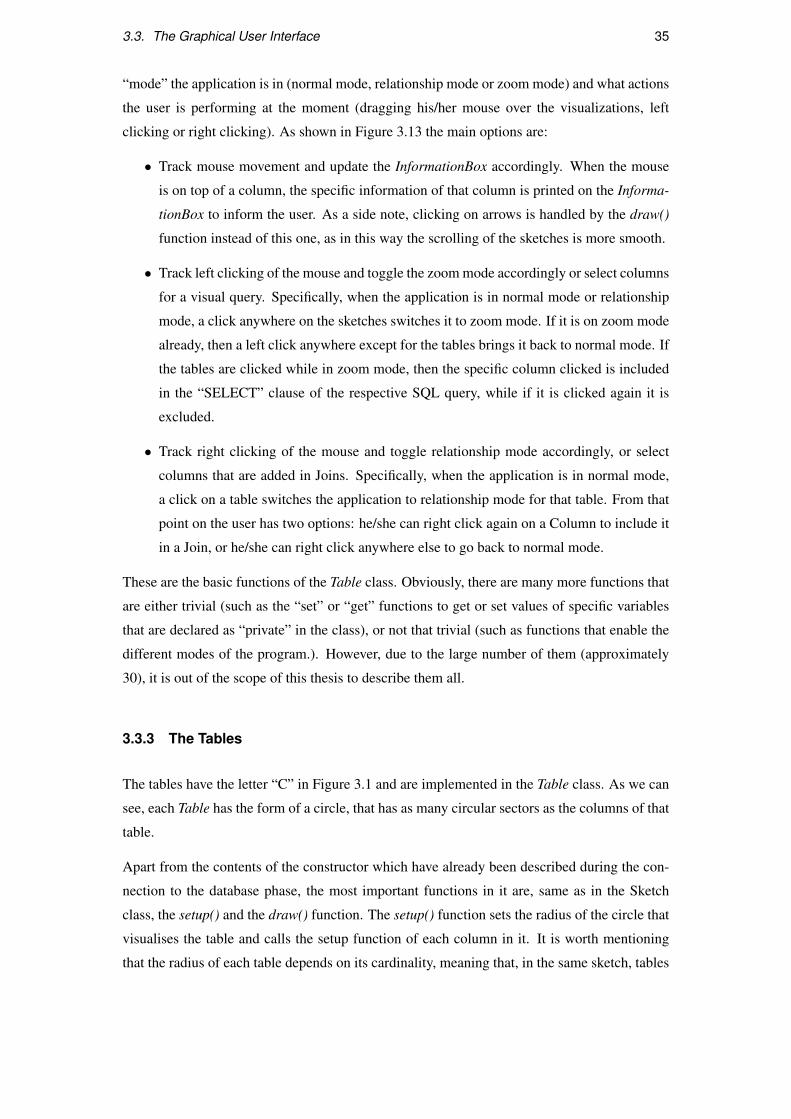
3.3.3 The Tables
The tables have the letter “C” in Figure 3.1 and are implemented in the Table class. As we can
see, each Table has the form of a circle, that has as many circular sectors as the columns of that
table.
Apart from the contents of the constructor which have already been described during the con-
nection to the database phase, the most important functions in it are, same as in the Sketch
class, the setup() and the draw() function. The setup() function sets the radius of the circle that
visualises the table and calls the setup function of each column in it. It is worth mentioning
that the radius of each table depends on its cardinality, meaning that, in the same sketch, tables

36 Chapter 3. Implementation
Figure 3.13: Code snippet with the mouseEvent function.
with fewer tuples will be visualised with a circle of smaller radius.
The draw() function performs sequential rotations of the coordinate system and calls the draw()
function of each of the columns residing in the table. It is worth mentioning that this is done
with the help of the pushMatrix() and popMatrix() functions as well. The pseudo-code in
Figure 3.14 presents the function in an abstract and more comprehensible way. As we notice,
the Table class, despite having a draw() function, it does not actually draw anything other than
the name of the table.
Figure 3.14: Pseudo-code with the Table.draw() function.
3.3. The Graphical User Interface 37
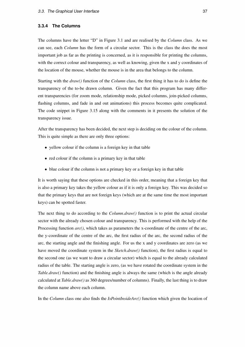
3.3.4 The Columns
The columns have the letter “D” in Figure 3.1 and are realised by the Column class. As we
can see, each Column has the form of a circular sector. This is the class the does the most
important job as far as the printing is concerned, as it is responsible for printing the columns,
with the correct colour and transparency, as well as knowing, given the x and y coordinates of
the location of the mouse, whether the mouse is in the area that belongs to the column.
Starting with the draw() function of the Column class, the first thing it has to do is define the
transparency of the to-be drawn column. Given the fact that this program has many differ-
ent transparencies (for zoom mode, relationship mode, picked columns, join-picked columns,
flashing columns, and fade in and out animations) this process becomes quite complicated.
The code snippet in Figure 3.15 along with the comments in it presents the solution of the
transparency issue.
After the transparency has been decided, the next step is deciding on the colour of the column.
This is quite simple as there are only three options:
• yellow colour if the column is a foreign key in that table
• red colour if the column is a primary key in that table
• blue colour if the column is not a primary key or a foreign key in that table
It is worth saying that these options are checked in this order, meaning that a foreign key that
is also a primary key takes the yellow colour as if it is only a foreign key. This was decided so
that the primary keys that are not foreign keys (which are at the same time the most important
keys) can be spotted faster.
The next thing to do according to the Column.draw() function is to print the actual circular
sector with the already chosen colour and transparency. This is performed with the help of the
Processing function arc(), which takes as parameters the x-coordinate of the centre of the arc,
the y-coordinate of the centre of the arc, the first radius of the arc, the second radius of the
arc, the starting angle and the finishing angle. For us the x and y coordinates are zero (as we
have moved the coordinate system in the Sketch.draw() function), the first radius is equal to
the second one (as we want to draw a circular sector) which is equal to the already calculated
radius of the table. The starting angle is zero, (as we have rotated the coordinate system in the
Table.draw() function) and the finishing angle is always the same (which is the angle already
calculated at Table.draw() as 360 degrees/number of columns). Finally, the last thing is to draw
the column name above each column.
In the Column class one also finds the IsPointInsideArc() function which given the location of
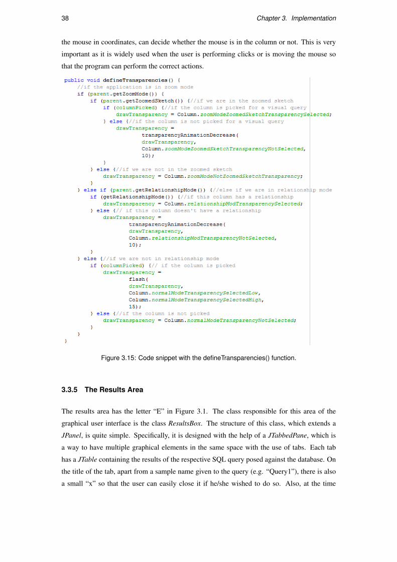
38 Chapter 3. Implementation
the mouse in coordinates, can decide whether the mouse is in the column or not. This is very
important as it is widely used when the user is performing clicks or is moving the mouse so
that the program can perform the correct actions.
Figure 3.15: Code snippet with the defineTransparencies() function.
3.3.5 The Results Area
The results area has the letter “E” in Figure 3.1. The class responsible for this area of the
graphical user interface is the class ResultsBox. The structure of this class, which extends a
JPanel, is quite simple. Specifically, it is designed with the help of a JTabbedPane, which is
a way to have multiple graphical elements in the same space with the use of tabs. Each tab
has a JTable containing the results of the respective SQL query posed against the database. On
the title of the tab, apart from a sample name given to the query (e.g. “Query1”), there is also
a small “x” so that the user can easily close it if he/she wished to do so. Also, at the time

3.3. The Graphical User Interface 39
the results table is created and put in a new tab, a new Table that represents graphically these
results is also created, as shown in Figure 2.9, and is then linked to its tab so that it can be used
in nested queries from now on. This new table disappears when the user closes the respective
tab in the results area.
The results are displayed with the help of a JTable, as already mentioned. With the help of
another class, RowNumberTable, the first column of the table is used for counting the number
of the rows in the result set. As soon as a query is executed and the results show up, the table
instantly scrolls to the end so that the user can see how many rows the results contain. Finally,
when the user hovers his/her mouse over a table with results, the SQL query used for that query
shows up, as shown in Figure 3.16.
Figure 3.16: The SQL query appears when the user hovers his mouse over the table.
3.3.6 The General Information Area
This area has the letter “F” in Figure 3.1 and is implemented by the InformationBox class. This
rectangular box at the right bottom of the graphical user interface consists of a JTextArea, a
Java class used for printing text on the screen. It has two different uses:
The first use this class has is displaying column characteristics when the mouse hovers above
a column. When this happens, the following details are printed on the screen:
• the name of the table
• the number of columns in this table
• the cardinality of this table
• the name of the column
• whether this column is a primary key
• whether this column is a foreign key
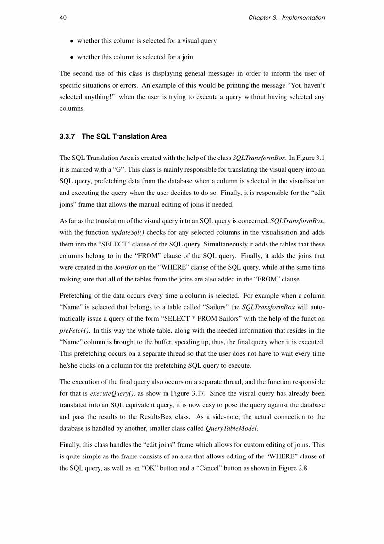
40 Chapter 3. Implementation
• whether this column is selected for a visual query
• whether this column is selected for a join
The second use of this class is displaying general messages in order to inform the user of
specific situations or errors. An example of this would be printing the message “You haven’t
selected anything!” when the user is trying to execute a query without having selected any
columns.
3.3.7 The SQL Translation Area
The SQL Translation Area is created with the help of the class SQLTransformBox. In Figure 3.1
it is marked with a “G”. This class is mainly responsible for translating the visual query into an
SQL query, prefetching data from the database when a column is selected in the visualisation
and executing the query when the user decides to do so. Finally, it is responsible for the “edit
joins” frame that allows the manual editing of joins if needed.
As far as the translation of the visual query into an SQL query is concerned, SQLTransformBox,
with the function updateSql() checks for any selected columns in the visualisation and adds
them into the “SELECT” clause of the SQL query. Simultaneously it adds the tables that these
columns belong to in the “FROM” clause of the SQL query. Finally, it adds the joins that
were created in the JoinBox on the “WHERE” clause of the SQL query, while at the same time
making sure that all of the tables from the joins are also added in the “FROM” clause.
Prefetching of the data occurs every time a column is selected. For example when a column
“Name” is selected that belongs to a table called “Sailors” the SQLTransformBox will auto-
matically issue a query of the form “SELECT * FROM Sailors” with the help of the function
preFetch(). In this way the whole table, along with the needed information that resides in the
“Name” column is brought to the buffer, speeding up, thus, the final query when it is executed.
This prefetching occurs on a separate thread so that the user does not have to wait every time
he/she clicks on a column for the prefetching SQL query to execute.
The execution of the final query also occurs on a separate thread, and the function responsible
for that is executeQuery(), as show in Figure 3.17. Since the visual query has already been
translated into an SQL equivalent query, it is now easy to pose the query against the database
and pass the results to the ResultsBox class. As a side-note, the actual connection to the
database is handled by another, smaller class called QueryTableModel.
Finally, this class handles the “edit joins” frame which allows for custom editing of joins. This
is quite simple as the frame consists of an area that allows editing of the “WHERE” clause of
the SQL query, as well as an “OK” button and a “Cancel” button as shown in Figure 2.8.
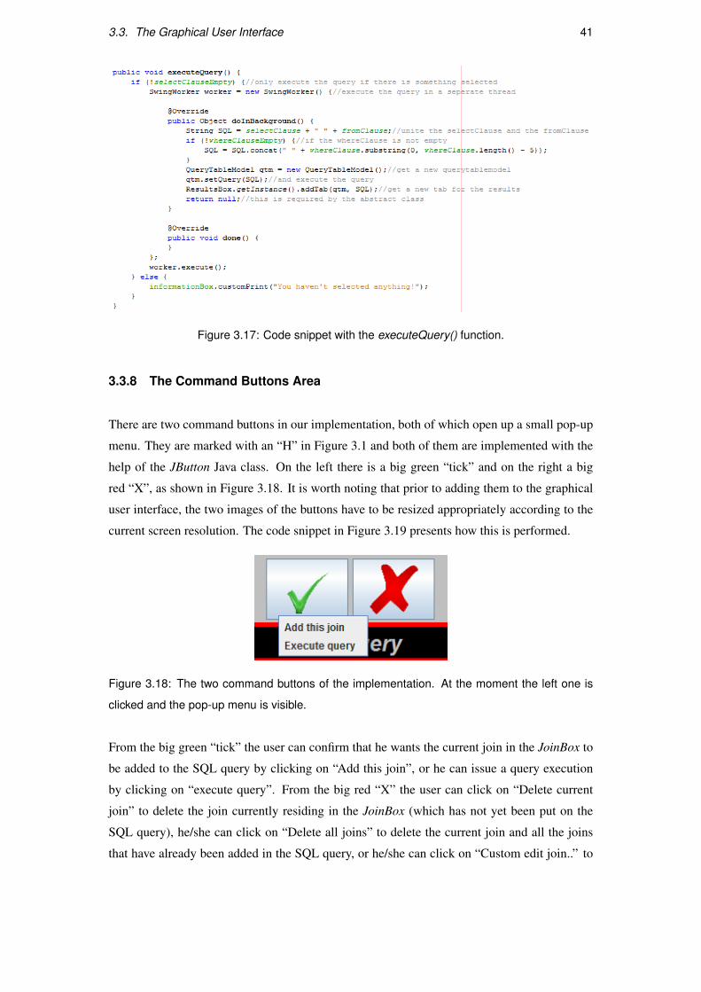
3.3. The Graphical User Interface 41
Figure 3.17: Code snippet with the executeQuery() function.
3.3.8 The Command Buttons Area
There are two command buttons in our implementation, both of which open up a small pop-up
menu. They are marked with an “H” in Figure 3.1 and both of them are implemented with the
help of the JButton Java class. On the left there is a big green “tick” and on the right a big
red “X”, as shown in Figure 3.18. It is worth noting that prior to adding them to the graphical
user interface, the two images of the buttons have to be resized appropriately according to the
current screen resolution. The code snippet in Figure 3.19 presents how this is performed.
Figure 3.18: The two command buttons of the implementation. At the moment the left one is
clicked and the pop-up menu is visible.
From the big green “tick” the user can confirm that he wants the current join in the JoinBox to
be added to the SQL query by clicking on “Add this join”, or he can issue a query execution
by clicking on “execute query”. From the big red “X” the user can click on “Delete current
join” to delete the join currently residing in the JoinBox (which has not yet been put on the
SQL query), he/she can click on “Delete all joins” to delete the current join and all the joins
that have already been added in the SQL query, or he/she can click on “Custom edit join..” to

42 Chapter 3. Implementation
Figure 3.19: Code snippet for resizing images so that they can be displayed correctly in any
resolution.
open up the “edit joins” window that has already been described.
All of these menu items that were described are implemented with the help of the Java class
JMenuItem and an ActionListener attached on each one of them. As shown in Figure 3.20
the actionListener is attached on a graphical object such as ours and can perform certain tasks
according to actions of the user (for example a button clicked).
Figure 3.20: The JMenuItem “ExecuteQuery” and its ActionListener.
3.3.9 The JoinBox Area
The JoinBox area is the last graphical object in our graphical user interface, and it is marked
with an “I” in Figure 3.1. It extends the JPanel class and has three objects in it: two JPanels and
a JComboBox. The two JPanels are by themselves containers for other objects. Specifically,
the left one has a JTextArea where information about the first column picked for a join appears,
while the second one has two elements that alternate places when needed with the help of a
very specific Java Layout called CardLayout. These two elements are a JTextArea to show the
same information that the left JTextArea shows and a JTextField in case the user wants to add a
specific constraint for a column (e.g. Age <30). As for the JComboBox element, this is where
the user can choose the relationship that he wants to exist among the two columns. The options
available are “<”, “>”, “=”, “>=”, “<=” or “! =”. Finally, when columns are picked for a
join and the Joinbox is full, two small “x” appear on top of the boxes, making it easy to empty
a box.

3.4. Launching from the Web 43
In general the functions in the JoinBox class mostly handle the contents of the two boxes,
making sure that they always get updated properly, no matter where they get updated from (the
small “x”on top, the CommandButton class, clicking on the visualisation itself). At the same
time this class produces the SQL String that is then added onto the “WHERE” clause of the
SQL query in the SQLTransformBox class.
3.4 Launching from the Web
After the application was created, it was decided to make it able to launch from the web as
well. The basic idea was that we would create a simple HTML page that would have a JApplet
in it. This JApplet is nothing else but a Java class that can be launched from an HTML page. In
this class there is only one button (created with a Java JButton), which when clicked launches
our graphical user interface. The only issue after this was to create a JAR file of our application
and sign it, as unsigned JAR files are not allowed to perform specific actions when they are
initiated as a JApplet from the web.
3.4.1 Creating the HTML Page
The HTML page that we created is a very simple one, as seen on Figure 2.2. In Figure 3.21
we can see the code of this html page. The line surrounded by the < applet > tags containts
the name of the starting class of the program - which in our case is the class AppletStart.java -
as well as all the libraries and pictures that out program uses. All of these files are also put in
the same folder where the HTML file should be (according to Xampp) so that they can be used
appropriately when needed.
Figure 3.21: The code for the Html page we built.

44 Chapter 3. Implementation
3.4.2 Signing the JAR File
Due to the problems occurring when an unsigned JAR is executing as a web application, the
signing of the JAR file had to be performed. The JDK (Java Development Kit) has two tools
that help in performing this action. The first one is the keytool, a key and certificate manage-
ment utility. It enables users to administer their own public/private key pairs and associated
certificates for use in self-authentication (where the user authenticates himself/herself to other
users/services) or data integrity and authentication services, using digital signatures. The sec-
ond one is the jarsigner, which can sign JAR files with the certificates produced by keytool,
or verify the validity of the certificates in a signed JAR file. After creating our certificate, we
signed our JAR file using the command “jarsigner Dissertation.jar -sakis”, where sakis is the
alias created by the keytool that links to our certificate.

Chapter 4
Evaluation
For the user-based evaluation of this program it was decided to use ten users. Despite the
fact that are evaluation mostly focuses on novice users that do not know how to use the SQL
language or Database Management Systems, it was also decided to use some people that had
experience with databases, in order to find any potential advantages that our platform offered
for them when compared to a DBMS. As such, five people that were familiar with databases
were chosen, and five that were not. Prior to the evaluation all of them were given a short, five
minute presentation of the system and its capabilities.
4.1 The Sample Database
In order to evaluate the implementation, a sample database had to be created. In this way the
users would be able to see all the features of the program and say whether they like them or
not, and at the same time perform certain tasks on that particular database so that the efficiency
of the new system could be measured and compared to the one of the DBMS system that we
used. For this job we decided to use a sample database that describes a DVD rental store, as
shown in Figure 4.1. This database consists of 15 tables, with multiple primary key - foreign
key relationships connecting them. The cardinality of the tables ranges from 2 tuples, up to
16,049. Finally, the tables column count range from 3 columns up to 13 columns.
4.2 The evaluation Form
The evaluation form consists of three parts: rating the system features, performing specific
tasks and counting the time required to do so, as well as overall commenting on the application
and its usefulness. As a side note, the third part of the evaluation form (the overall commenting)
45
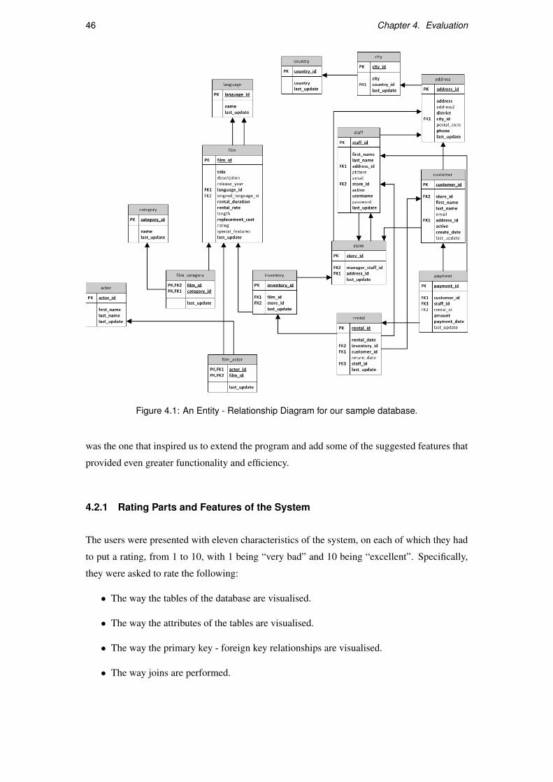
46 Chapter 4. Evaluation
Figure 4.1: An Entity - Relationship Diagram for our sample database.
was the one that inspired us to extend the program and add some of the suggested features that
provided even greater functionality and efficiency.
4.2.1 Rating Parts and Features of the System
The users were presented with eleven characteristics of the system, on each of which they had
to put a rating, from 1 to 10, with 1 being “very bad” and 10 being “excellent”. Specifically,
they were asked to rate the following:
• The way the tables of the database are visualised.
• The way the attributes of the tables are visualised.
• The way the primary key - foreign key relationships are visualised.
• The way joins are performed.
4.2. The evaluation Form 47
• The way that selected columns (that are put in the “SELECT” clause) are visualised.
• The way that selected columns for joins are visualised.
• System speed.
• System comprehensibility.
• Ease of use.
• Set of features (anything important missing?)
• Working without bugs?
4.2.2 Performing Tasks on the System
After that, the users were asked to perform certain tasks on our implementation, ranging from
very easy things to more complicated ones. Specifically, they were asked to:
• Open the database with name “Evaluation”.
• Write the primary key(s) of the table “Actor”.
• Write all the foreign keys of the table “Actor” along with their respective primary key
table and column.
• Write the cardinality of table “Customer”.
• Find all the first names of the Actors.
• Find the id of Actors that have first name “BEN”.
• Find in how many films the actors that have first name “BEN” have participated in.
At this point, the evaluation form provided offered an extra set of questions for people that were
familiar with databases. Those questions involved opening our Database Management System
(Microsoft SQL Server) and performing specific tasks on it, using the same sample database as
before. Specifically, the tasks they were asked to perform are the following:
• Find the cardinality of the “Payment” table.
• Find the primary keys of table “Customer”.
• Find all the foreign keys of the table “Customer” along with their respective primary key
table and column.
• List the category “names” with their “category ids”.
• Find the length and the actors of the file “ALABAMA DEVIL”.
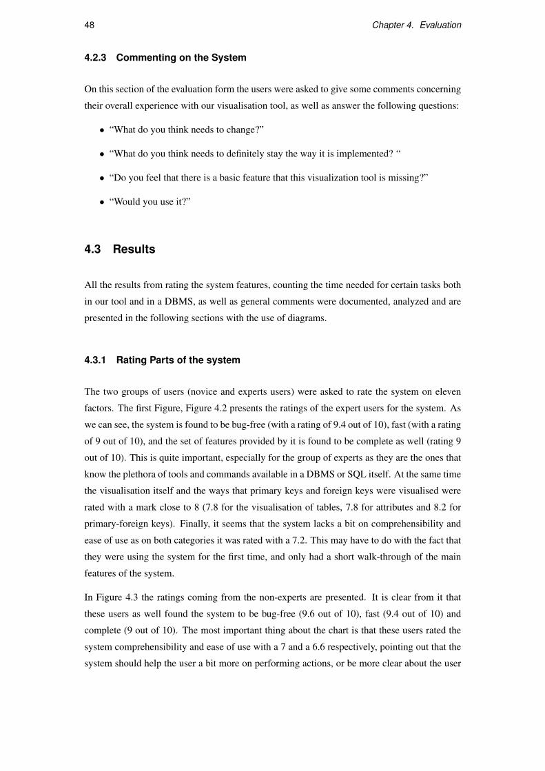
48 Chapter 4. Evaluation
4.2.3 Commenting on the System
On this section of the evaluation form the users were asked to give some comments concerning
their overall experience with our visualisation tool, as well as answer the following questions:
• “What do you think needs to change?”
• “What do you think needs to definitely stay the way it is implemented? “
• “Do you feel that there is a basic feature that this visualization tool is missing?”
• “Would you use it?”
4.3 Results
All the results from rating the system features, counting the time needed for certain tasks both
in our tool and in a DBMS, as well as general comments were documented, analyzed and are
presented in the following sections with the use of diagrams.
4.3.1 Rating Parts of the system
The two groups of users (novice and experts users) were asked to rate the system on eleven
factors. The first Figure, Figure 4.2 presents the ratings of the expert users for the system. As
we can see, the system is found to be bug-free (with a rating of 9.4 out of 10), fast (with a rating
of 9 out of 10), and the set of features provided by it is found to be complete as well (rating 9
out of 10). This is quite important, especially for the group of experts as they are the ones that
know the plethora of tools and commands available in a DBMS or SQL itself. At the same time
the visualisation itself and the ways that primary keys and foreign keys were visualised were
rated with a mark close to 8 (7.8 for the visualisation of tables, 7.8 for attributes and 8.2 for
primary-foreign keys). Finally, it seems that the system lacks a bit on comprehensibility and
ease of use as on both categories it was rated with a 7.2. This may have to do with the fact that
they were using the system for the first time, and only had a short walk-through of the main
features of the system.
In Figure 4.3 the ratings coming from the non-experts are presented. It is clear from it that
these users as well found the system to be bug-free (9.6 out of 10), fast (9.4 out of 10) and
complete (9 out of 10). The most important thing about the chart is that these users rated the
system comprehensibility and ease of use with a 7 and a 6.6 respectively, pointing out that the
system should help the user a bit more on performing actions, or be more clear about the user
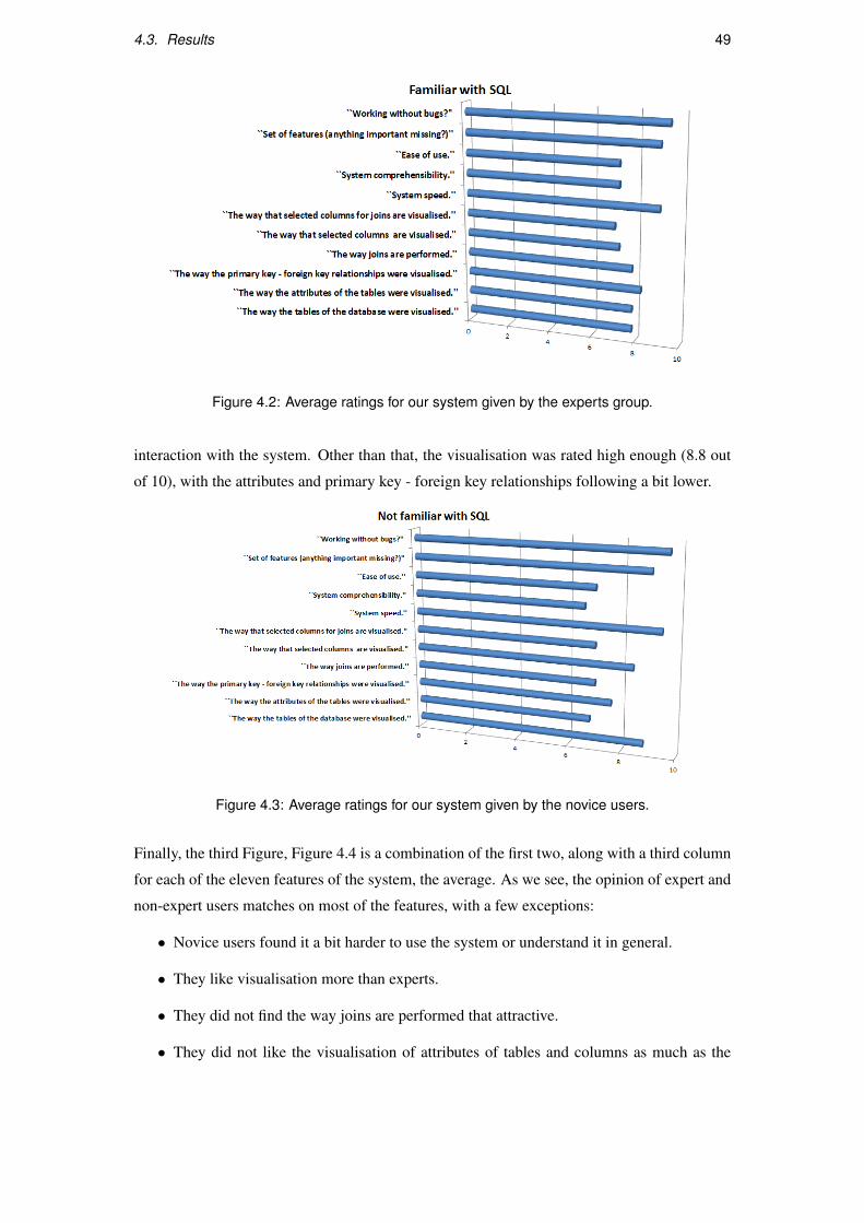
4.3. Results 49
Figure 4.2: Average ratings for our system given by the experts group.
interaction with the system. Other than that, the visualisation was rated high enough (8.8 out
of 10), with the attributes and primary key - foreign key relationships following a bit lower.
Figure 4.3: Average ratings for our system given by the novice users.
Finally, the third Figure, Figure 4.4 is a combination of the first two, along with a third column
for each of the eleven features of the system, the average. As we see, the opinion of expert and
non-expert users matches on most of the features, with a few exceptions:
• Novice users found it a bit harder to use the system or understand it in general.
• They like visualisation more than experts.
• They did not find the way joins are performed that attractive.
• They did not like the visualisation of attributes of tables and columns as much as the
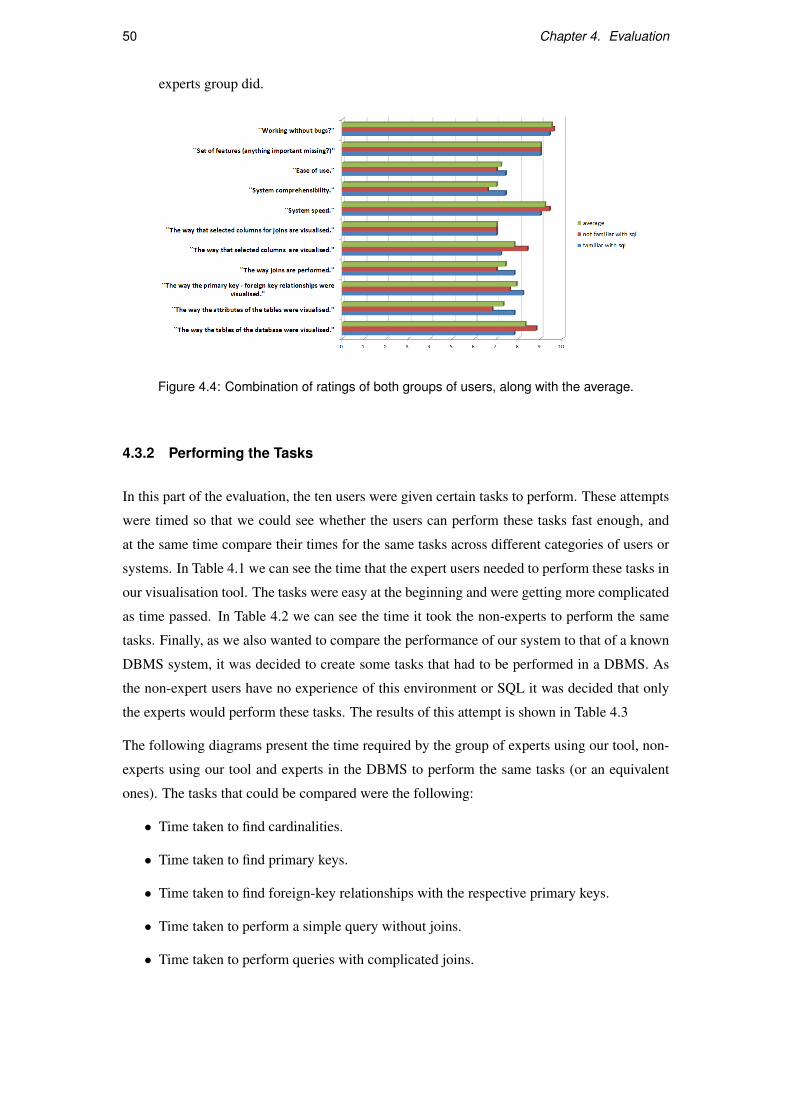
50 Chapter 4. Evaluation
experts group did.
Figure 4.4: Combination of ratings of both groups of users, along with the average.
4.3.2 Performing the Tasks
In this part of the evaluation, the ten users were given certain tasks to perform. These attempts
were timed so that we could see whether the users can perform these tasks fast enough, and
at the same time compare their times for the same tasks across different categories of users or
systems. In Table 4.1 we can see the time that the expert users needed to perform these tasks in
our visualisation tool. The tasks were easy at the beginning and were getting more complicated
as time passed. In Table 4.2 we can see the time it took the non-experts to perform the same
tasks. Finally, as we also wanted to compare the performance of our system to that of a known
DBMS system, it was decided to create some tasks that had to be performed in a DBMS. As
the non-expert users have no experience of this environment or SQL it was decided that only
the experts would perform these tasks. The results of this attempt is shown in Table 4.3
The following diagrams present the time required by the group of experts using our tool, non-
experts using our tool and experts in the DBMS to perform the same tasks (or an equivalent
ones). The tasks that could be compared were the following:
• Time taken to find cardinalities.
• Time taken to find primary keys.
• Time taken to find foreign-key relationships with the respective primary keys.
• Time taken to perform a simple query without joins.
• Time taken to perform queries with complicated joins.

4.3. Results 51
Tasks user1 user2 user3 user4 user5 average
Open the database named “Evaluation” 7 7 3 5 14 7.2
Write the primary keys of table “Actor” 6 28 5 6 37 16.4
Write the foreign keys of table “Actor”
along with their related primary keys 15 50 20 20 45 30
Write the cardinality of table “Customer” 4 52 9 15 9 17.8
Find the first names of all the actors 13 11 9 12 20 13
Find the ”id” of actors that
have a first name “BEN” 51 30 22 35 44 36.4
Find in how many films the actors with
first name “BEN” have participated in 80 95 114 120 138 109.4
Table 4.1: Time in seconds needed by each of the users in the experts group to perform the
tasks.
Tasks user6 user7 user8 user9 user10 average
Open the database named “Evaluation” 5 7 3 6 5 5.2
Write the primary keys of table “Actor” 19 22 37 17 12 21.4
Write the foreign keys of table “Actor”
along with their related primary keys 60 52 35 81 22 50
Write the cardinality of table “Customer” 7 4 28 41 19 19.8
Find the first names of all the actors 23 71 18 50 35 39.4
Find the ”id” of actors that
have a first name “BEN” 47 110 93 80 39 73.8
Find in how many films the actors with
first name “BEN” have participated in 188 164 300 300 224 235.2
Table 4.2: Time in seconds needed by each of the users in the non-experts group to perform
the tasks. The value “300” means that the particular user did not manage to finish on time or
finished with wrong results.

52 Chapter 4. Evaluation
Tasks user1 user2 user3 user4 user5 average
Find the cardinality of table “Payment” 45 50 35 14 45 37.8
Find the primary keys of table “Customer” 35 12 120 14 85 53.2
Find all the foreign keys of table
“Customer” along with their primary keys 117 125 300 99 123 152.8
Find the category names
with the category ids 27 53 70 35 70 51
Find the length and the actors
of the film “ALABAMA DEVIL” 130 135 216 81 136 139.6
Table 4.3: Time in seconds needed by each of the users in the expert group to perform the tasks.
The value “300” means that the particular user did not manage to finish on time or finished with
wrong results.
4.3.2.1 Time taken to find cardinalities
In Figure 4.5 the time required for our three different groups (experts in our tool, experts in
DBMS, non-experts in our tool) to find the cardinality of a table is presented. As we can
see from the diagram the time needed with the use of our tool is about the same for both
experts and non-experts (average of 17.8 seconds for experts and 19.8 for non experts) while
the time needed for experts in the DBMS we are using was 37.8 seconds. This equals to about
100% increase in the time needed when using the DBMS instead of our tool, and is probably
occurring due to the fact that the cardinalities of the tables in our visualisation tool appear just
by hovering the mouse over a table, while in a DBMS the user has to write an SQL query
(“SELECT COUNT(*) FROM ...”).
4.3.2.2 Time taken to find primary keys.
In Figure 4.6 the time required for our three different groups to find the primary keys of a table
is shown. As we can see, the time needed in our tool is again about the same for both experts
and non-experts (average of 16.4 seconds for experts and 21.4 for non experts) while the time
needed for experts in the DBMS was 53.2 seconds. This equals to about 180% increase in the
time needed when using the DBMS instead of our tool. This great difference in time needed
has a deeper cause: again in our tool all one needs to do is hover over a table to see the primary
keys, while in the DBMS one has to issue specific queries in the DBMS system tables (that are
DBMS-specific and will definitely take a lot of time), or he/she has to search for them in the
“Object Explorer”, the left bar of the program.

4.3. Results 53
Figure 4.5: Comparison of the time needed to find the cardinality of a table.
Figure 4.6: Comparison of the time needed to find the primary keys a table.
4.3.2.3 Time taken to find foreign-key relationships with the respective primary keys.
In Figure 4.7 the time required for our three different groups to find the foreign keys of a table
along with their respective primary keys and columns is shown. As we can see, the average
time needed by experts for this task in our tool was 30 seconds, the average time needed by
non-experts in our tool was 50 seconds and the average time needed for experts in a DBMS
was 152.8 seconds, including one user that did not manage to find them. As common as foreign
keys may be, it turned out to be quite complicated to find which tables and columns they relate
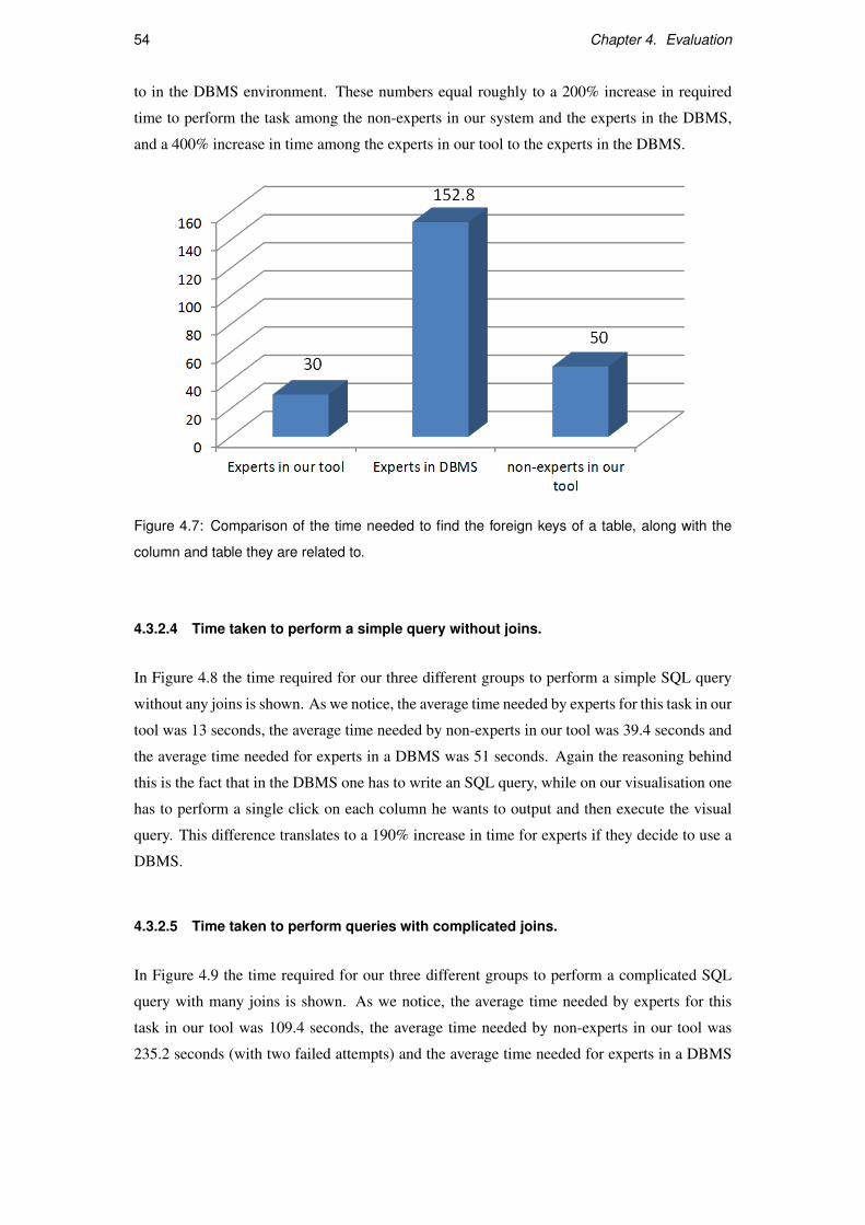
54 Chapter 4. Evaluation
to in the DBMS environment. These numbers equal roughly to a 200% increase in required
time to perform the task among the non-experts in our system and the experts in the DBMS,
and a 400% increase in time among the experts in our tool to the experts in the DBMS.
Figure 4.7: Comparison of the time needed to find the foreign keys of a table, along with the
column and table they are related to.
4.3.2.4 Time taken to perform a simple query without joins.
In Figure 4.8 the time required for our three different groups to perform a simple SQL query
without any joins is shown. As we notice, the average time needed by experts for this task in our
tool was 13 seconds, the average time needed by non-experts in our tool was 39.4 seconds and
the average time needed for experts in a DBMS was 51 seconds. Again the reasoning behind
this is the fact that in the DBMS one has to write an SQL query, while on our visualisation one
has to perform a single click on each column he wants to output and then execute the visual
query. This difference translates to a 190% increase in time for experts if they decide to use a
DBMS.
4.3.2.5 Time taken to perform queries with complicated joins.
In Figure 4.9 the time required for our three different groups to perform a complicated SQL
query with many joins is shown. As we notice, the average time needed by experts for this
task in our tool was 109.4 seconds, the average time needed by non-experts in our tool was
235.2 seconds (with two failed attempts) and the average time needed for experts in a DBMS
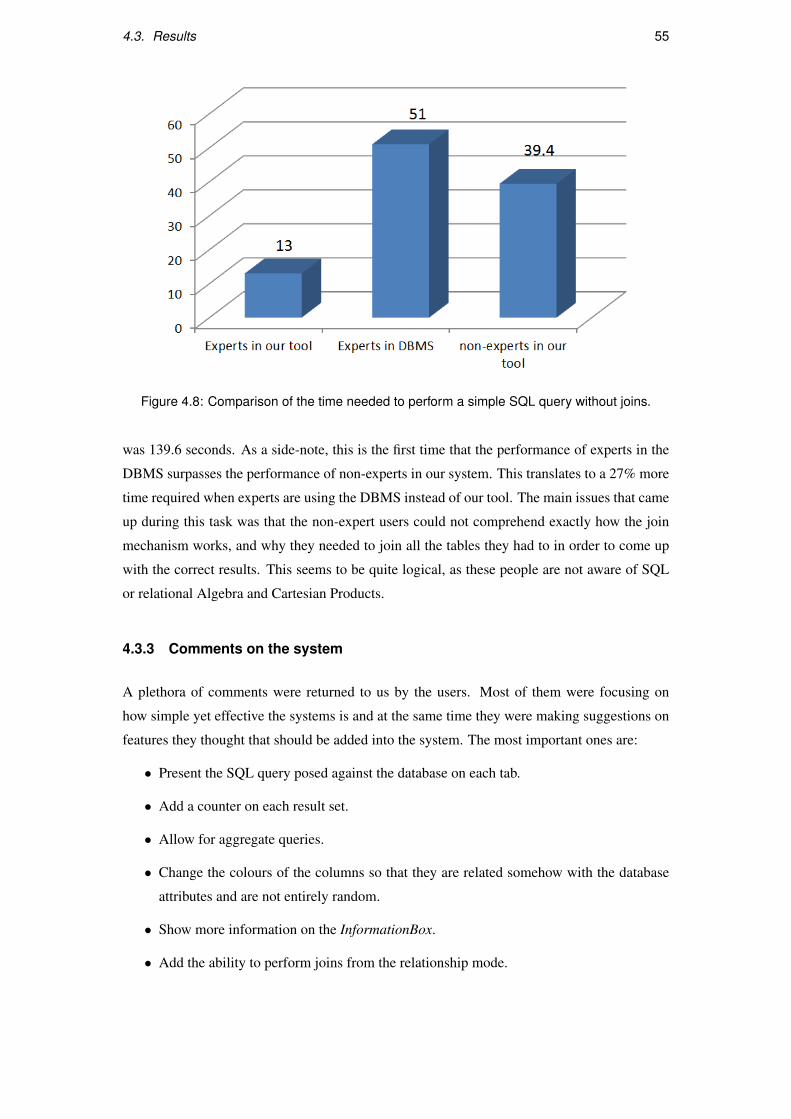
4.3. Results 55
Figure 4.8: Comparison of the time needed to perform a simple SQL query without joins.
was 139.6 seconds. As a side-note, this is the first time that the performance of experts in the
DBMS surpasses the performance of non-experts in our system. This translates to a 27% more
time required when experts are using the DBMS instead of our tool. The main issues that came
up during this task was that the non-expert users could not comprehend exactly how the join
mechanism works, and why they needed to join all the tables they had to in order to come up
with the correct results. This seems to be quite logical, as these people are not aware of SQL
or relational Algebra and Cartesian Products.
4.3.3 Comments on the system
A plethora of comments were returned to us by the users. Most of them were focusing on
how simple yet effective the systems is and at the same time they were making suggestions on
features they thought that should be added into the system. The most important ones are:
• Present the SQL query posed against the database on each tab.
• Add a counter on each result set.
• Allow for aggregate queries.
• Change the colours of the columns so that they are related somehow with the database
attributes and are not entirely random.
• Show more information on the InformationBox.
• Add the ability to perform joins from the relationship mode.

56 Chapter 4. Evaluation
Figure 4.9: Comparison of the time needed to perform a complicated SQL query with multiple
joins.
• Remodel the join box so that it is better looking.
• Provide hotkeys.
• Provide more information about what needs to be done, a wizard or something or some
examples.
• Drag and drop to make a join.
• Suggest joins automatically when needed.
Some of these features were added into the implementation on a later stage to provide
even more functionality.
4.4 Other Performance Tests
Apart from the tests described previously, some extra precaution measures were taken to make
sure that the implementation would work smoothly enough and would not affect by any means
the user experience due to poor performance. Specifically, the memory allocation for the pro-
gram was measured in order to make sure that there are no memory leaks. Also, special atten-
tion was given to the CPU utilization for every function in the program, to make sure that the
time spent on trivial tasks was minimal.
There are many tools out there to track memory allocation of objects and their life-cycle as
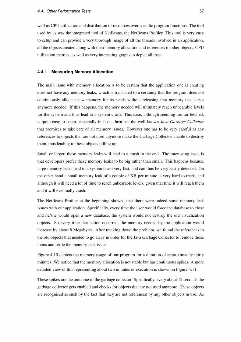
4.4. Other Performance Tests 57
well as CPU utilization and distribution of resources over specific program functions. The tool
used by us was the integrated tool of NetBeans, the NetBeans Profiler. This tool is very easy
to setup and can provide a very thorough image of all the threads involved in an application,
all the objects created along with their memory allocation and references to other objects, CPU
utilization metrics, as well as very interesting graphs to depict all these.
4.4.1 Measuring Memory Allocation
The main issue with memory allocation is to be certain that the application one is creating
does not have any memory leaks, which is translated to a certainty that the program does not
continuously allocate new memory for its needs without releasing first memory that is not
anymore needed. If this happens, the memory needed will ultimately reach unbearable levels
for the system and thus lead to a system crash. This case, although seeming too far-fetched,
is quite easy to occur, especially in Java. Java has the well-known Java Garbage Collector
that promises to take care of all memory issues. However one has to be very careful as any
references to objects that are not used anymore make the Garbage Collector unable to destroy
them, thus leading to these objects pilling up.
Small or larger, these memory leaks will lead to a crash in the end. The interesting issue is
that developers prefer these memory leaks to be big rather than small. This happens because
large memory leaks lead to a system crash very fast, and can thus be very easily detected. On
the other hand a small memory leak of a couple of KB per minute is very hard to track, and
although it will need a lot of time to reach unbearable levels, given that time it will reach them
and it will eventually crash.
The NetBeans Profiler at the beginning showed that there were indeed some memory leak
issues with our application. Specifically, every time the user would force the database to close
and he/she would open a new database, the system would not destroy the old visualization
objects. So every time that action occurred, the memory needed by the application would
increase by about 8 Megabytes. After tracking down the problem, we found the references to
the old objects that needed to go away in order for the Java Garbage Collector to remove those
items and settle the memory leak issue.
Figure 4.10 depicts the memory usage of our program for a duration of approximately thirty
minutes. We notice that the memory allocation is not stable but has continuous spikes. A more
detailed view of this representing about two minutes of execution is shown on Figure 4.11.
These spikes are the outcome of the garbage collector. Specifically, every about 17 seconds the
garbage collector gets enabled and checks for objects that are not used anymore. These objects
are recognised as such by the fact that they are not referenced by any other objects in use. As
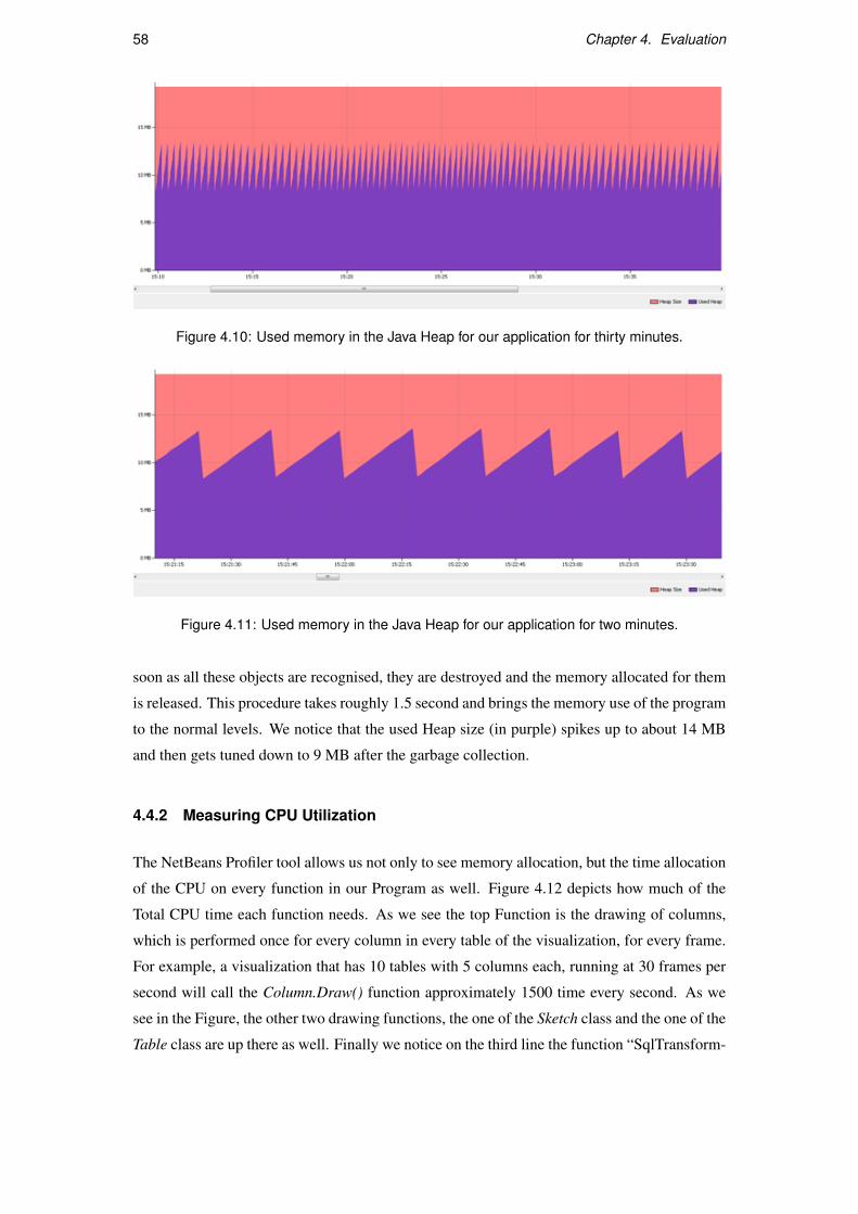
58 Chapter 4. Evaluation
Figure 4.10: Used memory in the Java Heap for our application for thirty minutes.
Figure 4.11: Used memory in the Java Heap for our application for two minutes.
soon as all these objects are recognised, they are destroyed and the memory allocated for them
is released. This procedure takes roughly 1.5 second and brings the memory use of the program
to the normal levels. We notice that the used Heap size (in purple) spikes up to about 14 MB
and then gets tuned down to 9 MB after the garbage collection.
4.4.2 Measuring CPU Utilization
The NetBeans Profiler tool allows us not only to see memory allocation, but the time allocation
of the CPU on every function in our Program as well. Figure 4.12 depicts how much of the
Total CPU time each function needs. As we see the top Function is the drawing of columns,
which is performed once for every column in every table of the visualization, for every frame.
For example, a visualization that has 10 tables with 5 columns each, running at 30 frames per
second will call the Column.Draw() function approximately 1500 time every second. As we
see in the Figure, the other two drawing functions, the one of the Sketch class and the one of the
Table class are up there as well. Finally we notice on the third line the function “SqlTransform-

4.4. Other Performance Tests 59
Box$1.doInBackground()” and on the fourth the “QueryTableModel.setQuery(String)”. These
functions both have to do with the execution of a query in the database that our program is
connected to with the help of JDBC, meaning that their duration depends on the very nature of
the query the user poses against the database. These functions may eventually reach the first
place on CPU utilization given long enough queries. As a side-note, these functions run on
separate threads, so that the user screen does not freeze while these execute.
Figure 4.12: Distribution of CPU time over the program’s functions.

Chapter 5
Conclusions
5.1 Summary
In this project the creation of a database visualisation tool was attempted. The tool created
managed to visualise a database in a clear and concise way, and at the same time offer to the
user the ability to perform visual queries. These queries translate to simple “SELECT-FROM-
WHERE” SQL queries, along with the ability of performing nested queries.
After the extended evaluation of the program it was found to be an overall functional tool, that
can help both experienced SQL users, as well as novice users. In most of the cases presented
in the study, the novice users using our tool would outperform expert users that were using the
DBMS, thing that points out the overall usefulness of this implementation. The main features
of the system seem to be clear enough and quite easy to use, with the exception of joins that
brought some annoyance in the non experts group. As a side-note, after the evaluation was
performed it was decided to implement some new features for the program, one of the being
the ability to perform joins straight from the “relationship mode”, hopefully reducing in this
way the problems that the novice users found when attempting to perform complicated SQL
queries.
5.2 Future Work
There are many extensions that can be performed in this project to further increase its function-
ality and ease of use. The most important thing that can be performed is extending the part of
the SQL language supported by the system, by allowing the use of aggregate functions (such as
AVERAGE, MIN, MAX etc). As these aggregate functions are used very often in SQL queries,
by supporting them the tool will attract more users. At the same time, as requested during the
61

62 Chapter 5. Conclusions
evaluation, including some “wizards” or documentation that demonstrate the basic functions
of the program will make the program more comprehensible. Finally, again as suggested by
users, the use of a drag and drop system to perform joins may increase the ease of use of the
system, and at the same time decrease the time needed to perform complicated SQL queries.
This program was built having in mind that it would not be used for vast databases. If that
becomes the case in the future, some modifications can be performed so that the user is able
to find a specific table in the visualisation faster. That could be done by adding a “Find a
table” option in the menu. At the same time a miniature representation of each sketch on the
visualisation showing which part of the sketch the user is viewing at the moment would help
navigation inside the sketch. Finally, it would be good if this program had a way to output the
results, either by printing them, or saving them in a file format. As a side-note, a print function
was created during the implementation, but was never added to the program. The code snippet
for that can be found on the Appendix.

Appendix A
Code snippets
Old method used for retrieving the names of the tables in the database:
1 String SQL ;
2 ResultSet rs ;
3 Statement stmt ;
4 stmt = connection . createStatement ( ) ;
5 SQL = ‘ ‘ SELECT name FROM sys . Tables ’ ’ ;
6 rs = stmt . executeQuery ( SQL ) ;
7 whi le ( rs . next ( ) )
8 {9 tableArray . add ( new Table ( rs . getString ( 1 ) ) ) ;
10 }
Old method for retrieving cardinality of each table:
1 SQL = ”SELECT c o u n t ( ∗ ) FROM ” + name ;
2 rs = stmt . executeQuery ( SQL ) ;
3 rs . next ( ) ;
4 cardinality = Integer . parseInt ( rs . getString ( 1 ) ) ;
Old method for retrieving the column names of each table:
1 SQL = ‘ ‘ SELECT COLUMN_NAME ‘ ‘
2 + ‘ ‘ FROM INFORMATION_SCHEMA . COLUMNS ’ ’
3 + ‘ ‘ WHERE TABLE_NAME= ’ ’ ’ + name + ‘ ‘ ’ ’ ’ ;
4 rs = stmt . executeQuery ( SQL ) ;
5 whi le ( rs . next ( ) )
6 {7 columnArray . add ( new Column ( rs . getString ( 1 ) , t h i s ) ) ;
8 }9 numberOfColumns = columnArray . size ( ) ;
63

64 Appendix A. Code snippets
Old method for retrieving primary keys:
1 f o r ( i n t i = 0 ; i < numberOfColumns ; i++)
2 {3 SQL = ‘ ‘ SELECT A . TABLE_NAME , A . COLUMN_NAME ’ ’
4 + ‘ ‘ FROM INFORMATION_SCHEMA . CONSTRAINT_COLUMN_USAGE as A , sys . key_constraints as
B ’ ’
5 + ‘ ‘ WHERE A . CONSTRAINT_NAME = B . name ’ ’
6 + ‘ ‘ AND TABLE_NAME= ’ ’ ’ + name + ‘ ‘ ’ ’ ’
7 + ‘ ‘ AND COLUMN_NAME= ’ ’ ’ + columnArray . g e t ( i ) . getName ( ) + ‘ ‘ ’ ’ ’ ;
8 rs = stmt . executeQuery ( SQL ) ;
9 whi le ( rs . next ( ) )
10 {11 columnArray . get ( i ) . setIsPrimaryKey ( ) ;
12 break ;
13 }14 }
Old method for retrieving foreign keys and their relationships:
1 f o r ( i n t i = 0 ; i < numberOfColumns ; i++)
2 {3 SQL = ‘ ‘ SELECT D . name , C . TABLE_NAME , C . COLUMN_NAME ‘ ‘
4 + ‘ ‘ FROM sys . objects AS A , sys . foreign_key_columns AS B , INFORMATION_SCHEMA .
COLUMNS AS C , sys . objects AS D ’ ’
5 + ‘ ‘ WHERE B . parent_object_id = A . object_id ’ ’
6 + ‘ ‘ AND C . TABLE_NAME = A . name ’ ’
7 + ‘ ‘ AND C . ORDINAL_POSITION = B . parent_column_id ’ ’
8 + ‘ ‘ AND D . object_id=referenced_object_id ’ ’
9 + ‘ ‘ AND TABLE_NAME= ’ ’ ’ + name + ‘ ‘ ’ ’ ’
10 + ‘ ‘ AND COLUMN_NAME= ’ ’ ’ + columnArray . g e t ( i ) . getName ( ) + ‘ ‘ ’ ’ ’ ;
11 rs = stmt . executeQuery ( SQL ) ;
12 whi le ( rs . next ( ) )
13 {14 columnArray . get ( i ) . setIsForeignKey ( rs . getString ( 1 ) ) ;
15 break ;
16 }17 SQL = ‘ ‘ SELECT c . TABLE_NAME , C . COLUMN_NAME , E . name ’ ’
18 + ‘ ‘ FROM SYS . foreign_key_columns AS A , SYS . objects AS B , INFORMATION_SCHEMA .
COLUMNS AS C , SYS . objects AS E ’ ’
19 + ‘ ‘ WHERE C . TABLE_NAME = B . name ’ ’
20 + ‘ ‘ AND B . object_id = A . referenced_object_id ’ ’
21 + ‘ ‘ AND C . ORDINAL_POSITION = A . referenced_column_id ’ ’
22 + ‘ ‘ AND E . object_id= A . parent_object_id ’ ’
23 + ‘ ‘ AND C . TABLE_NAME= ’ ’ ’ + name + ‘ ‘ ’ ’ ’
24 + ‘ ‘ AND C . COLUMN_NAME= ’ ’ ’ + columnArray . g e t ( i ) . getName ( ) + ‘ ‘ ’ ’ ’ ;
25 rs = stmt . executeQuery ( SQL ) ;
26 whi le ( rs . next ( ) )

65
27 {28 columnArray . get ( i ) . getRelatedForeignKeyTables ( ) . add ( rs . getString ( 3 ) ) ;
29 }30 }
Code snippet for printing the results of a tab:
1 p u b l i c vo id printCurrentTab ( )
2 {3 t r y4 {5 JScrollPane currentTabScrollPane = ( JScrollPane ) resultsTabs . getSelectedComponent
( ) ;
6 JViewport viewport = currentTabScrollPane . getViewport ( ) ;
7 JTable currentTabJTable = ( JTable ) viewport . getView ( ) ;
8 currentTabJTable . print ( JTable . PrintMode . FIT_WIDTH ) ;
9 } catch ( PrinterException ex )
10 {11 Exceptions . printStackTrace ( ex ) ;
12 }13 }


Bibliography
[1] Wikipedia Web Page. Database management systems. http://en.wikipedia.org/
wiki/Database_management_system, July 2011. Last Visited: August 2011.
[2] Wikipedia Web Page. Declarative programming. http://en.wikipedia.org/wiki/
Declarative_programming, June 2011. Last Visited: August 2011.
[3] D.D. Chamberlin and R.F. Boyce. Sequel: A structured english query language. In
Proceedings of the 1974 ACM SIGFIDET (now SIGMOD) workshop on Data description,
access and control, pages 249–264. ACM, 1974.
[4] D. Beech. Can sql3 be simplified? Database Programming and Design, 10:46–50, 1997.
[5] P.P. Chen. The entity-relationship model—toward a unified view of data. ACM Transac-
tions on database systems, 1(1):9–36, 1976.
[6] S.D. Viglas. Visual querying and exploration. 2005.
[7] J. Preece, Y. Rogers, and H. Sharp. Interaction design: Beyond human-computer interac-
tion. Wiley Dreamtech, 2003.
[8] M. Friendly. Milestones in the history of thematic cartography, statistical graphics, and
data visualization. Engineering, 9(2), 2008.
[9] J.W. Tukey. The future of data analysis. The Annals of Mathematical Statistics, 33(1):1–
67, 1962.
[10] D.P. Bickmore. Semiologie graphique: les diagrammes, les reseaux, les cartes, 1969.
[11] P. Madaiah. Database visualization. Master’s thesis, 2010.
[12] P. Chatzilidis. Database visualization. Master’s thesis, 2008.
[13] M.M. Zloof. Query by example. In Proceedings of the May 19-22, 1975, national com-
puter conference and exposition, pages 431–438. ACM, 1975.
67
68 Bibliography
[14] R. Ramakrishnan and J. Gehrke. Database Management Systems: International Edition.
McGraw-Hill, 2003.
[15] F. Benzi, D. Maio, and S. Rizzi. Visionary: a viewpoint-based visual language for query-
ing relational databases. Journal of Visual Languages and Computing, 10(2):117–145,
1999.
[16] M. Krzywinski. Schemaball webpage. http://mkweb.bcgsc.ca/schemaball/?home.
Last Visited: August 2011.
[17] M. Stonebraker, J. Chen, N. Nathan, C. Paxson, A. Su, and J. Wu. Tioga: A database-
oriented visualization tool. In Proceedings of the 4th conference on Visualization’93,
pages 86–93. IEEE Computer Society, 1993.
[18] A.A.J. Chen, M. Stonebraker, and A. Woodru. Tioga-2: A direct manipulation database
visualization environment.
[19] I.F. Cruz. Doodle: a visual language for object-oriented databases. In ACM SIGMOD
Record, volume 21, pages 71–80. ACM, 1992.
[20] I.F. Cruz. User-defined visual query languages. In Visual Languages, 1994. Proceedings.,
IEEE Symposium on, pages 224–231. IEEE, 1994.
[21] I.F. Cruz, M. Averbuch, W.T. Lucas, M. Radzyminski, and K. Zhang. Delaunay: a
database visualization system. In ACM SIGMOD Record, volume 26, pages 510–513.
ACM, 1997.
[22] Processing Web Page. www.processing.org. Last Visited: August 2011.
[23] G. Reese and A. Oram. Database Programming with JDBC and JAVA. O’Reilly &
Associates, Inc., 2000.
[24] K.O. Seidler. Xampp web page. http://www.apachefriends.org/en/xampp.html,
January 2011. Last Visited: August 2011.
[25] Jarsigner Online Documentation. jarsigner - jar signing and verification tool. http://
download.oracle.com/javase/1.3/docs/tooldocs/win32/jarsigner.html. Last
Visited: August 2011.
Related Documents