Database Support for Enabling Data-Discovery Queries over Semantically-Annotated Observational Data Huiping Cao 1 , Shawn Bowers 2 , and Mark P. Schildhauer 3 1 Dept. of Computer Science, New Mexico State University [email protected] 2 Dept. of Computer Science, Gonzaga University [email protected] 3 NCEAS, University of California Santa Barbara [email protected] Abstract. Observational data plays a critical role in many scientific disciplines, and scientists are increasingly interested in performing broad-scale analyses by using observational data collected as part of many smaller scientific studies. How- ever, while these data sets often contain similar types of information, they are typically represented using very different structures and with little semantic infor- mation about the data itself, which creates significant challenges for researchers who wish to discover existing data sets based on data semantics (observation and measurement types) and data content (the values of measurements within a data set). We present a formal framework to address these challenges that consists of a semantic observational model (to uniformly represent observation and mea- surement types), a high-level semantic annotation language (to map tabular re- sources into the model), and a declarative query language that allows researchers to express data-discovery queries over heterogeneous (annotated) data sets. To demonstrate the feasibility of our framework, we also present implementation approaches for efficiently answering discovery queries over semantically anno- tated data sets. In particular, we propose two storage schemes (in-place databases rdb and materialized databases mdb) to store the source data sets and their annota- tions. We also present two query schemes (ExeD and ExeH) to evaluate discovery queries and the results of extensive experiments comparing their effectiveness. 1 Introduction Accessing and reusing observational data is essential for performing scientific anal- yses at broad geographic, temporal, and biological scales. Classic examples in earth and environmental science include examining the effects of nitrogen treatments across North American grasslands [20], and studying how changing environmental conditions affect bird migratory patterns [22]. These types of studies often require access to hun- dreds of data sets collected by independent research groups over many years. Tools that aim to help researchers discover and reuse these data sets must overcome a number of This work was supported in part through NSF grants DBI-0743429 and DBI-0753144, and NMSU Interdisciplinary Research Grant #111721. A. Hameurlain et al. (Eds.): TLDKS VI , LNCS 7600, pp. 198–228, 2012. c Springer-Verlag Berlin Heidelberg 2012

Welcome message from author
This document is posted to help you gain knowledge. Please leave a comment to let me know what you think about it! Share it to your friends and learn new things together.
Transcript

Database Support for Enabling Data-Discovery Queriesover Semantically-Annotated Observational Data!
Huiping Cao1, Shawn Bowers2, and Mark P. Schildhauer3
1 Dept. of Computer Science, New Mexico State [email protected]
2 Dept. of Computer Science, Gonzaga [email protected]
3 NCEAS, University of California Santa [email protected]
Abstract. Observational data plays a critical role in many scientific disciplines,and scientists are increasingly interested in performing broad-scale analyses byusing observational data collected as part of many smaller scientific studies. How-ever, while these data sets often contain similar types of information, they aretypically represented using very different structures and with little semantic infor-mation about the data itself, which creates significant challenges for researcherswho wish to discover existing data sets based on data semantics (observation andmeasurement types) and data content (the values of measurements within a dataset). We present a formal framework to address these challenges that consistsof a semantic observational model (to uniformly represent observation and mea-surement types), a high-level semantic annotation language (to map tabular re-sources into the model), and a declarative query language that allows researchersto express data-discovery queries over heterogeneous (annotated) data sets. Todemonstrate the feasibility of our framework, we also present implementationapproaches for efficiently answering discovery queries over semantically anno-tated data sets. In particular, we propose two storage schemes (in-place databasesrdb and materialized databases mdb) to store the source data sets and their annota-tions. We also present two query schemes (ExeD and ExeH) to evaluate discoveryqueries and the results of extensive experiments comparing their effectiveness.
1 Introduction
Accessing and reusing observational data is essential for performing scientific anal-yses at broad geographic, temporal, and biological scales. Classic examples in earthand environmental science include examining the effects of nitrogen treatments acrossNorth American grasslands [20], and studying how changing environmental conditionsaffect bird migratory patterns [22]. These types of studies often require access to hun-dreds of data sets collected by independent research groups over many years. Tools thataim to help researchers discover and reuse these data sets must overcome a number of
! This work was supported in part through NSF grants DBI-0743429 and DBI-0753144, andNMSU Interdisciplinary Research Grant #111721.
A. Hameurlain et al. (Eds.): TLDKS VI , LNCS 7600, pp. 198–228, 2012.c! Springer-Verlag Berlin Heidelberg 2012
Database Support for Enabling Data-Discovery Queries 199
site plt size ph spp len dbh
GCE6 A 7 4.5 piru 21.6 36.0GCE6 B 8 4.8 piru 27.0 45... ... ... ... ... ... ...GCE7 A 7 3.7 piru 23.4 39.1GCE7 B 8 3.9 piru 25.2 42.7... ... ... ... ... ... ...
yr field area acidity piru abba ...
2005 f1 5 5.1 20.8 14.1 ...2006 f1 5 5.2 21.1 15.2 ...... ... ... ... ... ... ...2010 f1 5 5.8 22.0 18.9 ...2005 f2 7 4.9 18.9 15.3 ...... ... ... ... ... ... ...
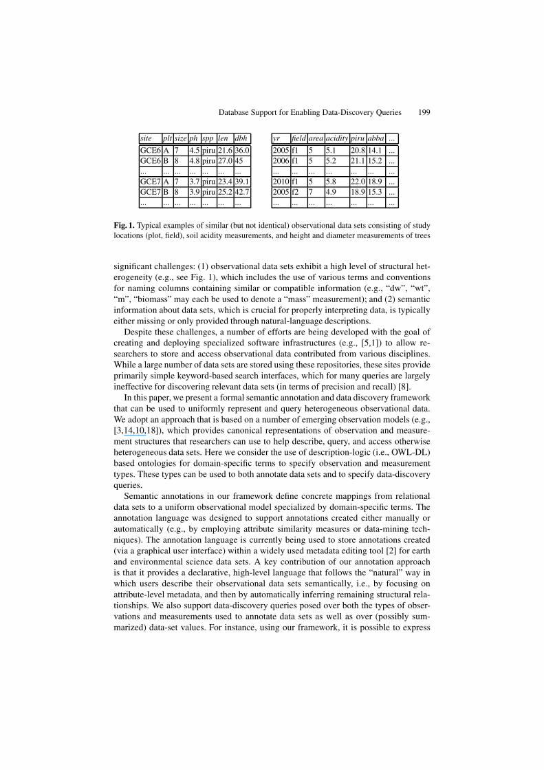
Fig. 1. Typical examples of similar (but not identical) observational data sets consisting of studylocations (plot, field), soil acidity measurements, and height and diameter measurements of trees
significant challenges: (1) observational data sets exhibit a high level of structural het-erogeneity (e.g., see Fig. 1), which includes the use of various terms and conventionsfor naming columns containing similar or compatible information (e.g., “dw”, “wt”,“m”, “biomass” may each be used to denote a “mass” measurement); and (2) semanticinformation about data sets, which is crucial for properly interpreting data, is typicallyeither missing or only provided through natural-language descriptions.
Despite these challenges, a number of efforts are being developed with the goal ofcreating and deploying specialized software infrastructures (e.g., [5,1]) to allow re-searchers to store and access observational data contributed from various disciplines.While a large number of data sets are stored using these repositories, these sites provideprimarily simple keyword-based search interfaces, which for many queries are largelyineffective for discovering relevant data sets (in terms of precision and recall) [8].
In this paper, we present a formal semantic annotation and data discovery frameworkthat can be used to uniformly represent and query heterogeneous observational data.We adopt an approach that is based on a number of emerging observation models (e.g.,[3,14,10,18]), which provides canonical representations of observation and measure-ment structures that researchers can use to help describe, query, and access otherwiseheterogeneous data sets. Here we consider the use of description-logic (i.e., OWL-DL)based ontologies for domain-specific terms to specify observation and measurementtypes. These types can be used to both annotate data sets and to specify data-discoveryqueries.
Semantic annotations in our framework define concrete mappings from relationaldata sets to a uniform observational model specialized by domain-specific terms. Theannotation language was designed to support annotations created either manually orautomatically (e.g., by employing attribute similarity measures or data-mining tech-niques). The annotation language is currently being used to store annotations created(via a graphical user interface) within a widely used metadata editing tool [2] for earthand environmental science data sets. A key contribution of our annotation approachis that it provides a declarative, high-level language that follows the “natural” way inwhich users describe their observational data sets semantically, i.e., by focusing onattribute-level metadata, and then by automatically inferring remaining structural rela-tionships. We also support data-discovery queries posed over both the types of obser-vations and measurements used to annotate data sets as well as over (possibly sum-marized) data-set values. For instance, using our framework, it is possible to express
200 H. Cao, S. Bowers, and M.P. Schildhauer
queries that range from simple “schema-level” filters such as “Find all data sets thatcontain height measurements of trees within experimental locations” to queries that ac-cess, summarize, and select results based on the values within data sets such as “Findall data sets that have trees with a maximum height measurement larger than 20 mwithin experimental locations having an area smaller than 10 m2”.
Finally, we describe different storage and query evaluation approaches that have beenimplemented to support the framework. We consider two main approaches. The first isa “data warehouse” approach that uses a single “materialized” database to store un-derlying observational data sets, where query evaluation involves rewriting a discoveryquery into a query over the warehouse. In the second approach, semantic annotations aretreated as logical views over the underlying data set schemas, where query evaluationinvolves rewriting the original query using the annotation into corresponding queriesover the underlying data sets. Based on our initial experimental results, we demonstratethe feasibility of querying a large corpus using these approaches, and that querying datain place can lead to better performance compared with more traditional warehousingapproaches. This paper is an extended version of [11] that describes in detail queryevaluation strategies for complex data-discovery queries and additional correspondingexperimental results.
The rest of this paper is organized as follows. In Sect. 2 we present the observa-tional model, semantic annotation language, and data-discovery language used withinour framework. In Sect. 3 we describe implementation approaches. In Sect. 4 we presentour experimental results. In Sect. 5 we discuss related work, and in Sect. 6 we summa-rize our contributions.
2 Semantic Annotation and Discovery Framework
Fig. 2 shows the modeling constructs we use to describe and (depending on the imple-mentation) store observational data. An observation is made of an entity (e.g., biologicalorganisms, geographic locations, or environmental features, among others) and primar-ily serves to group a set of measurements together to form a single “observation event”.A measurement assigns a value to a characteristic of the observed entity (e.g., the heightof a tree), where a value is denoted through another entity (which includes primitive val-ues such as integers and strings, similar to pure object-oriented models). Measurementsalso include standards (e.g., units) for relating values across measurements, and canalso specify additional information including collection protocols, methods, precision,and accuracy (not all of which are shown in Fig. 2). An observation (event) can occurwithin the context of zero or more other observations. Context can be viewed as a formof dependency, e.g., an observation of a tree specimen may have been made within aspecific geographic location, and the geographic location provides important informa-tion for interpreting and comparing tree measurements. In this case, by establishing acontext relationship between the tree and location observations, the measured valuesof the location are assumed to be constant with respect to the measurements of thetree (i.e., the tree measurements are dependent on the location measurements). Contextforms a transitive relationship among observations. Although not considered here, wealso employ a number of additional structures in the model for representing complex

Database Support for Enabling Data-Discovery Queries 201
!"#$%&
'()*)+$,*-.#+&
/0.,*1)#2"&
3,).4*,5,"$&
6*2$2+27&
8$)"9)*9&
().3,).4*,5,"$&
2:'()*)+$,*-.#+&
4.,.6*2$2+27&
4.,.8$)"9)*9&
2:!"#$%&
().'2"$,;$&
<==<&>&
<==<&
>&
>&
>&<==<&
<==<&
<==<&>&
>&
().?)74,&
<==<&
>&
>&
Fig. 2. Main observational modeling constructs used in semantic annotation and data discovery
units, characteristics, and named relationships between observations and entities [10].When describing data sets using the model of Fig. 2, domain-specific entity, character-istic, and standard classes are typically used. That is, our framework allows subclassesof the classes in Fig. 2 to be defined and related, and these terms can then be used whendefining semantic annotations.
A key feature of the model is its ability for users to assert properties of entities (asmeasurement characteristics or contextual relationships) without requiring these prop-erties to be interpreted as inherently (i.e., always) true of the entity. Depending on thecontext an entity was observed (or how measurements were performed), its propertiesmay take on different values. For instance, the diameter of a tree changes over time,and the diameter value often depends on the protocol used to obtain the measurement.The observation and measurement structure of Fig. 2 allows RDF-style assertions aboutentities while allowing for properties to be contextualized (i.e., the same entity can havedifferent values for a characteristic under different contexts), which is a crucial featurefor modeling scientific data [10]. Although shown using UML in Fig. 2, the model hasbeen implemented (together with a number of domain extensions) using OWL-DL.1
2.1 Semantic Annotation
Semantic annotations are represented using a high-level annotation language in whicheach annotation consists of two separate parts: (1) a semantic template that definesspecific observation and measurement types (and their various relationships) for thedata set; and (2) a mapping from individual attributes of a data set to measurementtypes defined within the semantic template. A semantic template consists of one ormore observation types O specified using statements of the form
O ::= Observation [ {distinct} ] ido : EntType [ , ContextType ]! [ MeasType ]!
where square brackets denote optional elements and ! denotes repetition. In particular,an observation type consists of an optional distinct constraint, a name (denoted idO),an entity type, zero or more context types, and zero or more measurement types. Entity,context, and measurement types are specified using the following syntax
1 e.g., see http://ecoinformatics.org/oboe/oboe.1.0/oboe-core.owl
202 H. Cao, S. Bowers, and M.P. Schildhauer
EntType ::= Entity =e
ContextType ::= Context [ {identifying} ] = ido
MeasType ::= Measurement [ {key} ] idm : Characteristic =c [ , Standard =s ]
where e, c, and s are respectively entity, characteristic, and standard types (e.g., drawnfrom an OWL ontology), ido is an observation type name (defined within the sameannotation), and idm is a measurement type name. Both the optional identifying and keykeywords represent constraints, which together with the distinct constraint, are definedfurther below. A mapping M , which links data-set attributes to measurement types,takes the form
M ::= Map a to idm [ , a to idm ]!
where a is an attribute name within the data set and idm is a measurement type name(defined in the template).
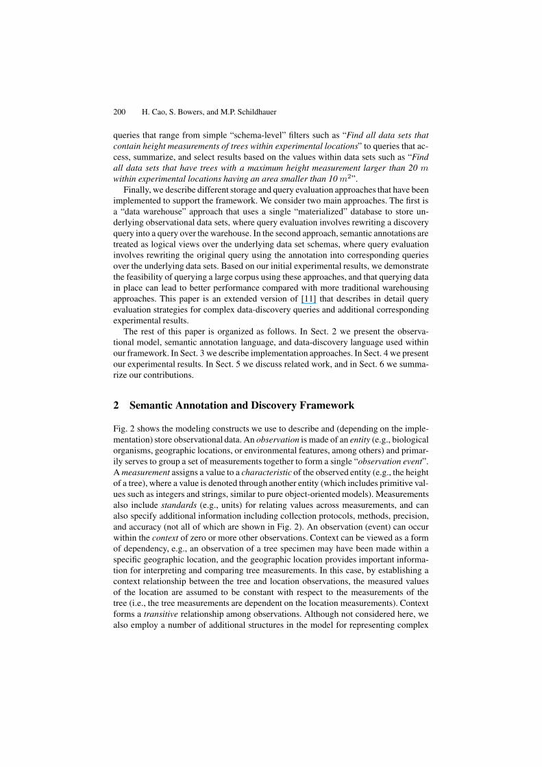
The left side of Fig. 3 gives an example annotation for the first table of Fig. 1. Herewe define four observation types denoting measurements of sites, plots, soils, and trees,respectively. A site observation contains a simple (so-called “nominal”) measurementthat gives the name of the site. Similarly, a plot observation records the name of the plot(where a plot is used as an experimental replicate) as well as the plot area. Here, plotsare observed within the context of a corresponding site. A soil observation consists ofan acidity measurement and is made within the context of a plot observation (althoughnot shown, we would typically label the context relation in this case to denote that thesoil is part of the plot). A tree observation consists of the taxonomic name of the treealong with height and diameter measurements in meters and centimeters, respectively.Finally, each attribute in the data set of Fig. 1 is mapped (via the Map statement) to itscorresponding measurement type.
The right side of Fig. 3 gives a visual representation of the relationship between (aportion of) the semantic template (top) and the attribute mapping (dashed-lines, middle)
Observation {distinct} ot1: Entity = Site
Measurement {key} mt1: Characteristic = Name
Observation {distinct} ot2 : Entity = Plot, Context {identifying} = ot1
Measurement {key} mt2: Characteristic = Name
Measurement {key} mt3: Characteristic = Area, Standard = MeterSquare
Observation ot3: Entity = Soil, Context = ot2
Measurement mt4: Characteristic = Acidity, Standard = pH
Observation ot4: Entity = Tree, Context {identifying} = ot2
Measurement {key} mt5: Characteristic = TaxonName
Measurement mt6: Characteristic = Height, Standard = Meter
Measurement mt7: Characteristic = Diameter, Standard = Centimeter
Map site to mt1, plt to mt2, size to mt3, ph to mt4, spp to mt5, len to mt6,
dbh to mt7
site plt size ph …
!"#$
%&'($
)(*#$
+*,($
!"#$
-./'$
!"#$
%/&.$
)(*#$
+*,($
)(*#$ )(*#$
01&2&'3$
45$,6$
07(*$
Semantic Template Semantic Annotation
Dataset Schema
Fig. 3. Semantic annotation of the first data set of Fig. 1 showing the high-level annotation syn-tax (left) and a graphical representation of the corresponding “semantic template” and column-mapping (right)
Database Support for Enabling Data-Discovery Queries 203
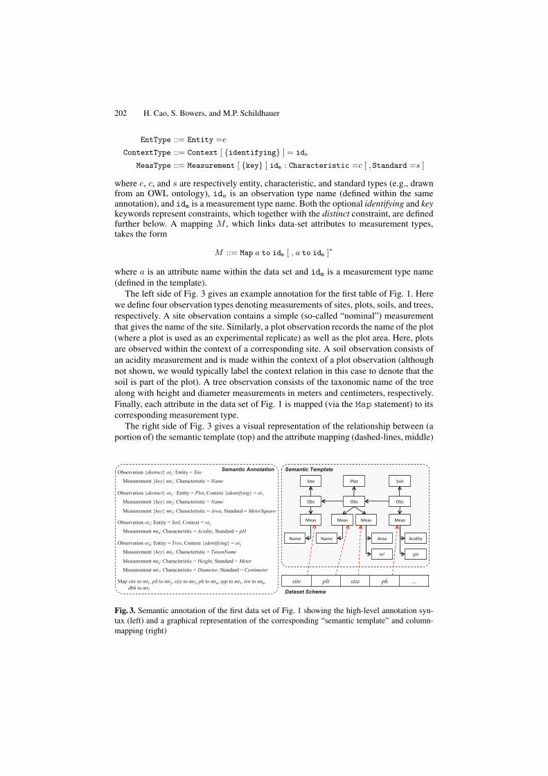
Fig. 4. The semantic annotation user interface developed within the Morpho metadata editor
from the underlying data set schema (bottom) to the template. The visual representa-tion of the template informally matches the observational model shown in Fig. 2, wherearrows denote relationships between classes. As shown, each attribute is assigned toa single measurement type in the template. This approach follows the typical view ofattributes in data sets as specifying measurements, where the corresponding entities,observation events, and context relationships are implied by the template. To help usersspecify semantic annotations, we have also developed a graphical user-interface within[2] that allows users to specify attribute-level mappings to measurement types and thecorresponding measurement and observation types of the data set. An example of theinterface is shown in Fig. 4 in which the measurement associated with the column la-beled “WET” is being specified. The annotation language is used to store (via an XMLserialization) the mappings and semantic templates generated by the interface.
The meaning of a semantic annotation can be viewed as the result of processing adata set row-by-row such that each row creates a valid instance of the semantic template.We refer to such an instance as a materialization of the data set with respect to the an-notation. For example, in the first row of the data set as in Fig. 1, the site value “GCE6”implies: (1) an instance m1 of the measurement type mt1 whose value is “GCE6”; (2)an instance c1 of the Name characteristic for m1; (3) an instance o1 of an observation(corresponding to type ot1) having measurement m1; and (4) an instance e1 of the Siteentity such that e1 is the entity of o1. Similarly, assuming the plot attribute value “A”of the first row corresponds to an observation instance o2 (of observation type ot2), thecontext definition for ot2 results in o2 having o1 as context.
The key, identifying, and distinct constraints are used to further specify the structureof semantic-template instances. These constraints are similar to key and weak-entity

204 H. Cao, S. Bowers, and M.P. Schildhauer
constraints used within ER models. If a measurement type is defined as a key (e.g., mt1in Fig. 3), then the values of instances for these measurement types identify the cor-responding observation entity (similar to key attributes in an ER model). For example,consider the first table in Fig. 1. Both the first and the second row have the same sitevalue of “GCE6”. Let e1 be the entity instance of the first-row’s corresponding observa-tion. Let o1 and o3 be the observation instances for the site attribute in the first row andthe second row respectively. The key constraint of mt1 requires that e1 be an entity ofboth o1 and o3. Similarly, an identifying constraint requires the identity of one observa-tion’s entity to depend (through context) on the identity of another observation’s entity(similar to identifying relationships in an ER model). In our example, plot names areunique only within a corresponding site. Thus, a plot with name “A” in one site is not thesame plot as a plot with name “A” in a different site. Identifying constraints define thatthe identity of an observation’s entity is determined by both its own key measurementsand its identifying observations’ key measurements.
Definition 1 (Key measurement types). The set of key measurement types Keys(O)of an observation type O are the measurement types whose values can distinguish oneentity instance (of which the observation is made) from another. Given an observationtype O, let Mkeys(O) be the set of measurement types of O that are specified with a keyconstraint. Similarly, let Cid(O) be the set of context observation types of O that arespecified with an identifying constraint. The set of key measurement types of O are thus
Keys(O) = Mkeys(O) " {M | O! # Cid(O) $M # Keys(O!)}.
Example 1 (Key measurement type example). Given the semantic annotation in Fig. 3,we can derive the key measurement types for the observation types. First, ot1’s keymeasurement type is {mt1} because (a) ot1 does not have any identifying constraint,and (b) ot1’s direct key measurement type is mt1. Second, ot2’s key measurement typesare {mt3,mt2,mt1} because (a) ot1 is the identifying constraint of ot2, (b) ot1’s keymeasurement type is mt1, and (c) ot2’s direct measurement key types are mt2 and mt3.Similarly, we can derive that ot4’s key measurement types are {mt5,mt3,mt2,mt1}.
The distinct constraint on observations is similar to a key constraint on measurements,except that it is used to uniquely identify observations (as opposed to observation en-tities). Distinct constraints can only be used if each measurement of the observationis constrained to be a key. Specifically, for a given set of key measurement values ofan observation type specified to be distinct, the set of measurement values uniquelyidentifies an observation instance. Thus, for any particular set of measurement values,there will be only one corresponding observation instance. In Fig. 3, each row with thesame value for the site attribute maps not only to the same observed entity (via the keyconstraint) but also to the same observation instance (via the distinct constraint).
Materialization Relations. Given a data set and an annotation, we materialize the dataset with respect to the annotation into a set of relation instances. We represent annota-tions using the following schema.
– Annot(a, d) states that a is an annotation of data set with id d.– ObsType(a, ot, et, isDistinct) states that ot is an observation type in annotation a,
has entity type et, and whether it is declared as having the distinct constraint.
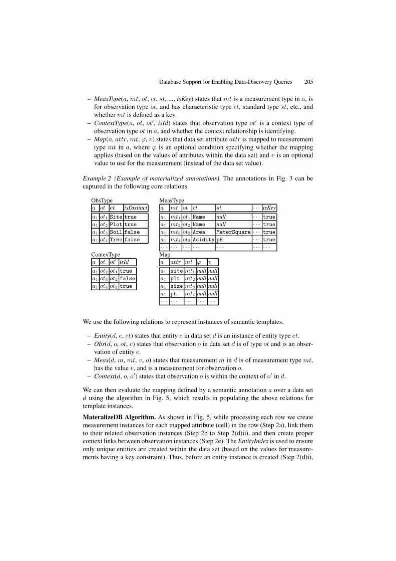
Database Support for Enabling Data-Discovery Queries 205
– MeasType(a, mt, ot, ct, st, ..., isKey) states that mt is a measurement type in a, isfor observation type ot, and has characteristic type ct, standard type st, etc., andwhether mt is defined as a key.
– ContextType(a, ot, ot!, isId) states that observation type ot! is a context type ofobservation type ot in a, and whether the context relationship is identifying.
– Map(a, attr, mt, !, v) states that data set attribute attr is mapped to measurementtype mt in a, where ! is an optional condition specifying whether the mappingapplies (based on the values of attributes within the data set) and v is an optionalvalue to use for the measurement (instead of the data set value).
Example 2 (Example of materialized annotations). The annotations in Fig. 3 can becaptured in the following core relations.
ObsTypea ot et isDistinct
a1 ot1 Site true
a1 ot2 Plot true
a1 ot3 Soil false
a1 ot4 Tree false
MeasTypea mt ot ct st · · · isKey
a1 mt1 ot1 Name null · · · truea1 mt2 ot2 Name null · · · truea1 mt3 ot2 Area MeterSquare · · · truea1 mt4 ot3 Acidity pH · · · true· · · · · · · · · · · · · · · · · · · · ·
ContexTypea ot ot" isId
a1 ot2 ot1 true
a1 ot3 ot2 false
a1 ot4 ot2 true
Mapa attr mt ! v
a1 site mt1 null nulla1 plt mt2 null nulla1 size mt3 null nulla1 ph mt4 null null· · · · · · · · · · · · · · ·
We use the following relations to represent instances of semantic templates.
– Entity(d, e, et) states that entity e in data set d is an instance of entity type et.– Obs(d, o, ot, e) states that observation o in data set d is of type ot and is an obser-
vation of entity e.– Meas(d, m, mt, v, o) states that measurement m in d is of measurement type mt,
has the value v, and is a measurement for observation o.– Context(d, o, o!) states that observation o is within the context of o! in d.
We can then evaluate the mapping defined by a semantic annotation a over a data setd using the algorithm in Fig. 5, which results in populating the above relations fortemplate instances.
MateralizeDB Algorithm. As shown in Fig. 5, while processing each row we createmeasurement instances for each mapped attribute (cell) in the row (Step 2a), link themto their related observation instances (Step 2b to Step 2(d)ii), and then create propercontext links between observation instances (Step 2e). The EntityIndex is used to ensureonly unique entities are created within the data set (based on the values for measure-ments having a key constraint). Thus, before an entity instance is created (Step 2(d)i),
206 H. Cao, S. Bowers, and M.P. Schildhauer
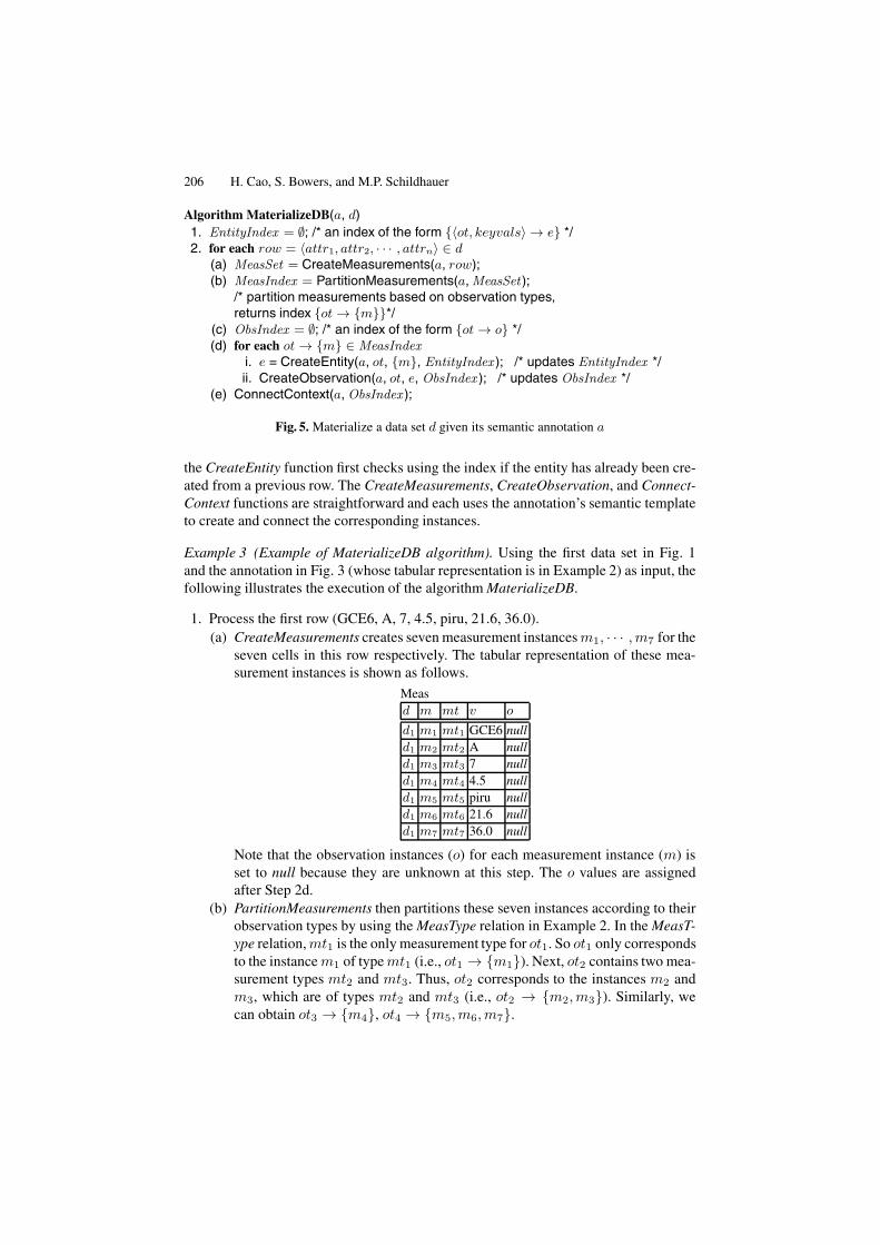
Algorithm MaterializeDB(a, d)1. EntityIndex = !; /* an index of the form {"ot, keyvals# $ e} */2. for each row = "attr1, attr2, · · · , attrn# % d
(a) MeasSet = CreateMeasurements(a, row);(b) MeasIndex = PartitionMeasurements(a, MeasSet );
/* partition measurements based on observation types,returns index {ot $ {m}}*/
(c) ObsIndex = !; /* an index of the form {ot $ o} */(d) for each ot $ {m} % MeasIndex
i. e = CreateEntity(a, ot, {m}, EntityIndex ); /* updates EntityIndex */ii. CreateObservation(a, ot, e, ObsIndex ); /* updates ObsIndex */
(e) ConnectContext(a, ObsIndex );
Fig. 5. Materialize a data set d given its semantic annotation a
the CreateEntity function first checks using the index if the entity has already been cre-ated from a previous row. The CreateMeasurements, CreateObservation, and Connect-Context functions are straightforward and each uses the annotation’s semantic templateto create and connect the corresponding instances.
Example 3 (Example of MaterializeDB algorithm). Using the first data set in Fig. 1and the annotation in Fig. 3 (whose tabular representation is in Example 2) as input, thefollowing illustrates the execution of the algorithm MaterializeDB.
1. Process the first row (GCE6, A, 7, 4.5, piru, 21.6, 36.0).(a) CreateMeasurements creates seven measurement instancesm1, · · · ,m7 for the
seven cells in this row respectively. The tabular representation of these mea-surement instances is shown as follows.
Measd m mt v o
d1 m1 mt1 GCE6 nulld1 m2 mt2 A nulld1 m3 mt3 7 nulld1 m4 mt4 4.5 nulld1 m5 mt5 piru nulld1 m6 mt6 21.6 nulld1 m7 mt7 36.0 null
Note that the observation instances (o) for each measurement instance (m) isset to null because they are unknown at this step. The o values are assignedafter Step 2d.
(b) PartitionMeasurements then partitions these seven instances according to theirobservation types by using the MeasType relation in Example 2. In the MeasT-ype relation,mt1 is the only measurement type for ot1. So ot1 only correspondsto the instance m1 of typemt1 (i.e., ot1 % {m1}). Next, ot2 contains two mea-surement types mt2 and mt3. Thus, ot2 corresponds to the instances m2 andm3, which are of types mt2 and mt3 (i.e., ot2 % {m2,m3}). Similarly, wecan obtain ot3 % {m4}, ot4 % {m5,m6,m7}.
Database Support for Enabling Data-Discovery Queries 207
Entityd e et
d1 e1 Sited1 e2 Plotd1 e3 Soild1 e4 Tree
Obsd o ot e
d1 o1 ot1 e1d1 o2 ot2 e2d1 o3 ot3 e3d1 o4 ot4 e4
Measd m mt v o
d1 m1 mt1 GCE6 o1d1 m2 mt2 A o2d1 m3 mt3 7 o2d1 m4 mt4 4.5 o3d1 m5 mt5 piru o4d1 m6 mt6 21.6 o4d1 m7 mt7 36.0 o4
Contextd o o"
d1 o2 o1d1 o3 o2d1 o4 o2
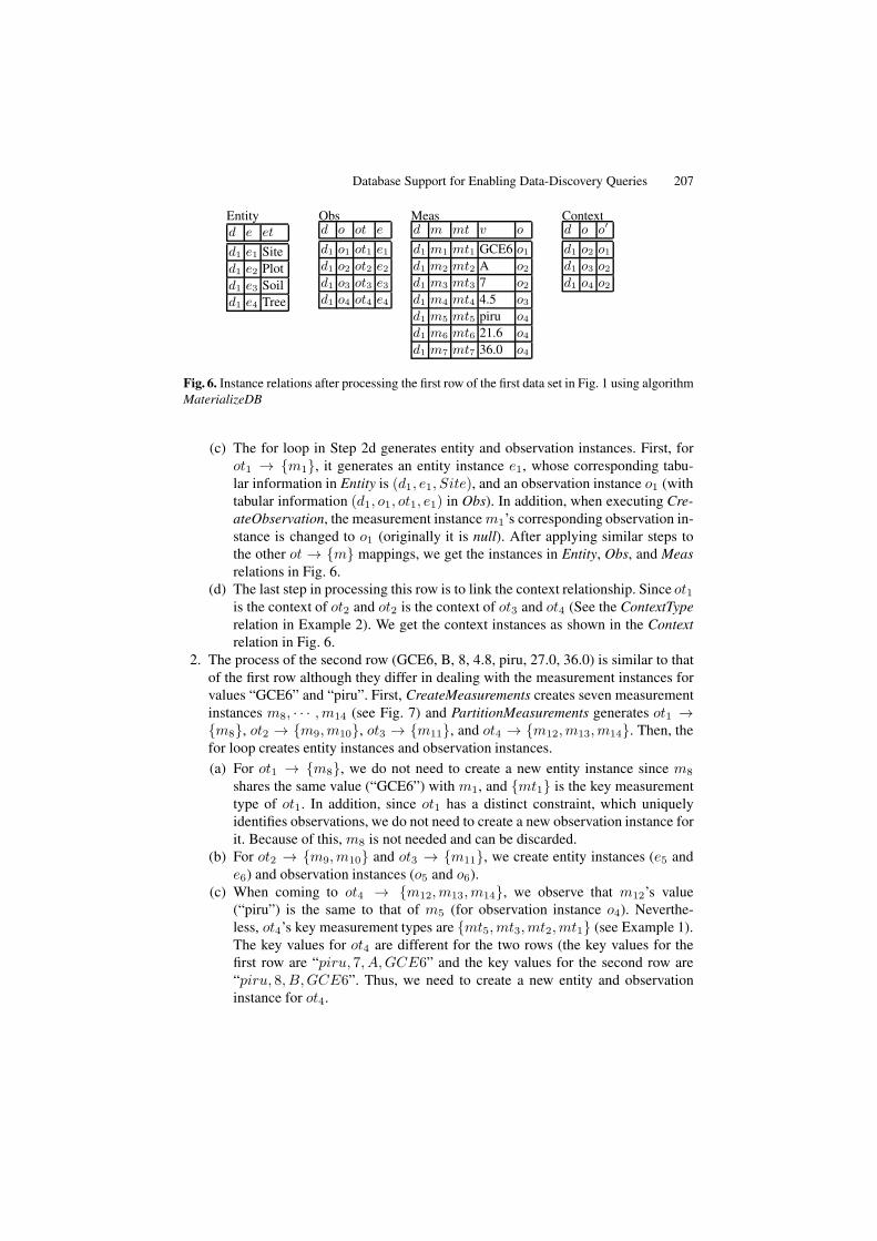
Fig. 6. Instance relations after processing the first row of the first data set in Fig. 1 using algorithmMaterializeDB
(c) The for loop in Step 2d generates entity and observation instances. First, forot1 % {m1}, it generates an entity instance e1, whose corresponding tabu-lar information in Entity is (d1, e1, Site), and an observation instance o1 (withtabular information (d1, o1, ot1, e1) in Obs). In addition, when executing Cre-ateObservation, the measurement instance m1’s corresponding observation in-stance is changed to o1 (originally it is null). After applying similar steps tothe other ot % {m} mappings, we get the instances in Entity, Obs, and Measrelations in Fig. 6.
(d) The last step in processing this row is to link the context relationship. Since ot1is the context of ot2 and ot2 is the context of ot3 and ot4 (See the ContextTyperelation in Example 2). We get the context instances as shown in the Contextrelation in Fig. 6.
2. The process of the second row (GCE6, B, 8, 4.8, piru, 27.0, 36.0) is similar to thatof the first row although they differ in dealing with the measurement instances forvalues “GCE6” and “piru”. First, CreateMeasurements creates seven measurementinstances m8, · · · ,m14 (see Fig. 7) and PartitionMeasurements generates ot1 %{m8}, ot2 % {m9,m10}, ot3 % {m11}, and ot4 % {m12,m13,m14}. Then, thefor loop creates entity instances and observation instances.(a) For ot1 % {m8}, we do not need to create a new entity instance since m8
shares the same value (“GCE6”) with m1, and {mt1} is the key measurementtype of ot1. In addition, since ot1 has a distinct constraint, which uniquelyidentifies observations, we do not need to create a new observation instance forit. Because of this, m8 is not needed and can be discarded.
(b) For ot2 % {m9,m10} and ot3 % {m11}, we create entity instances (e5 ande6) and observation instances (o5 and o6).
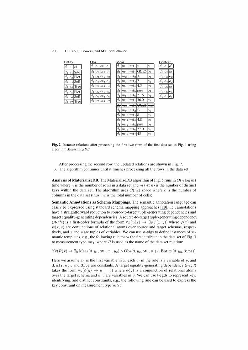
(c) When coming to ot4 % {m12,m13,m14}, we observe that m12’s value(“piru”) is the same to that of m5 (for observation instance o4). Neverthe-less, ot4’s key measurement types are {mt5,mt3,mt2,mt1} (see Example 1).The key values for ot4 are different for the two rows (the key values for thefirst row are “piru, 7, A,GCE6” and the key values for the second row are“piru, 8, B,GCE6”. Thus, we need to create a new entity and observationinstance for ot4.
208 H. Cao, S. Bowers, and M.P. Schildhauer
Entityd e et
d1 e1 Sited1 e2 Plotd1 e3 Soild1 e4 Tree
d1 e5 Plotd1 e6 Soild1 e7 Tree
Obsd o ot e
d1 o1 ot1 e1d1 o2 ot2 e2d1 o3 ot3 e3d1 o4 ot4 e4
d1 o5 ot2 e5d1 o6 ot3 e6d1 o7 ot4 e7
Measd m mt v o
d1 m1 mt1 GCE6 o1d1 m2 mt2 A o2d1 m3 mt3 7 o2d1 m4 mt4 4.5 o3d1 m5 mt5 piru o4d1 m6 mt6 21.6 o4d1 m7 mt7 36.0 o4
d1 m8 mt1 GCE6 nulld1 m9 mt2 B o5d1 m10 mt3 8 o5d1 m11 mt4 4.8 o6d1 m12 mt5 piru o7d1 m13 mt6 27.0 o7d1 m14 mt7 45 o7
Contextd o o"
d1 o2 o1d1 o3 o2d1 o4 o2
d1 o5 o1d1 o6 o5d1 o7 o5
Fig. 7. Instance relations after processing the first two rows of the first data set in Fig. 1 usingalgorithm MaterializeDB
After processing the second row, the updated relations are shown in Fig. 7.3. The algorithm continues until it finishes processing all the rows in the data set.
Analysis of MaterializeDB. The MaterializeDB algorithm of Fig. 5 runs in O(n logm)time where n is the number of rows in a data set and m (& n) is the number of distinctkeys within the data set. The algorithm uses O(nc) space where c is the number ofcolumns in the data set (thus, nc is the total number of cells).
Semantic Annotations as Schema Mappings. The semantic annotation language caneasily be expressed using standard schema mapping approaches [19], i.e., annotationshave a straightforward reduction to source-to-target tuple-generating dependencies andtarget equality-generating dependencies. A source-to-target tuple-generating dependency(st-tdg) is a first-order formula of the form 'x(!(x) % (y "(x, y)) where !(x) and"(x, y) are conjunctions of relational atoms over source and target schemas, respec-tively, and x and y are tuples of variables. We can use st-tdgs to define instances of se-mantic templates, e.g., the following rule maps the first attribute in the data set of Fig. 3to measurement type mt1, where R is used as the name of the data set relation:
'x(R(x) % (yMeas(d, y1, mt1, x1, y2) $Obs(d, y2, ot1, y3) $ Entity(d, y3, Site))
Here we assume x1 is the first variable in x, each yi in the rule is a variable of y, andd, mt1, ot1, and Site are constants. A target equality-generating dependency (t-egd)takes the form 'y(#(y) % u = v) where #(y) is a conjunction of relational atomsover the target schema and u, v are variables in y. We can use t-egds to represent key,identifying, and distinct constraints, e.g., the following rule can be used to express thekey constraint on measurement type mt1:
Database Support for Enabling Data-Discovery Queries 209
'y(Meas(d,m1, mt1, v, o1) $Obs(d, o1, ot1, e1) $Meas(d,m2, mt1, v, o2)$Obs(d, o2, ot1, e2) % e1 = e2)
The annotation language we employ is also similar to a number of other high-levelmapping languages used for data exchange (e.g., [13,6]), but supports simple type as-sociations to attributes (e.g., as shown by the red arrows on the right of Fig. 3) whileproviding well-defined and unambiguous mappings from data sets to the observationand measurement schema.
2.2 Data Discovery Queries
Data discovery queries can be used to select relevant data sets based on their observationand measurement types and values. A basic discovery query Q takes the form
Q ::= EntityType(Condition)
where EntityType is a specific entity OWL class and Condition is a conjunction ordisjunction of zero or more conditions. A condition takes the form
Condition ::= CharType [ op value [ StandardType ] ]
| f(CharType) [ op value [ StandardType ] ]
| count( [ distinct ] &) op value
where CharType and StandardType are specific characteristic and (measurement)standard OWL classes, respectively, and f denotes an aggregation function (sum, avg,min, or max). A data set is returned by a basic discovery query if it contains obser-vations of the given entity type that satisfy the corresponding conditions. We considerthree basic types of conditions (for the three syntax rules above): (1) the observationmust contain at least one measurement of a given characteristic type (CharType) witha measured value satisfying a relational (i.e., =, )=, >, <, *, +) or string comparison(e.g., contains); (2) the aggregate function applied to measurements of the character-istic type (CharType) for all observations of the entity type must satisfy the relationalcomparison; and (3) the number (count) of all observations of the entity type mustsatisfy the relational comparison (where distinct restricts the set of observations tothose within unique entities). For instance, in the following basic discovery queries
Tree(TaxonName = ‘piru’)Tree(TaxonName = ‘piru’ ' count(distinct &) ( 5)
the first query selects data sets with at least one Tree observation labeled as having the(abbreviated) taxon name “piru”, and the second query restricts the returned data setsof the first query to contain at least five such observations.
A contextualized discovery query generalizes basic discovery queries to allow selec-tions on context. A contextualized query QC for n * 1 has the form
QC ::= Q1 $ Q2 · · · $ Qn
where each Qi is a basic discovery query and % denotes a context relationship. A dataset satisfies a contextualized query if it satisfies each basic query Qi and each matching

210 H. Cao, S. Bowers, and M.P. Schildhauer
Qi is related by the given context constraint. In a contextualized query, there exists atmost one aggregation function in a basic query. In addition, since each Qi has Qi+1 asits context, the entity of Q1 is logically contained in its context queries’ entities. So, theaggregation condition applies to Q1 (the finest level of entity) if QC has an aggregationcondition. To illustrate, the following examples can be used to express the two queriesof Sect. 1:
Tree(Height) $ Plot()Tree(max(height) ( 20 Meter) $ Plot(area < 10 MeterSquare).
That is, the first query returns data sets that contain height measurements of trees withinplots (experimental locations), and the second returns data sets that have trees of amaximum height larger than 20 m within plots having an area smaller than 10 m2. Fora collection of data sets D and a contextualized discovery query Q, in the normal way,we write Q(D) to denote the subset of data sets in D that satisfy Q. Note that Q(D) canbe computed on a per data set basis, i.e., by checking each data set in D individually tosee whether it satisfies Q.
3 Approaches for Evaluating Data Discovery Queries
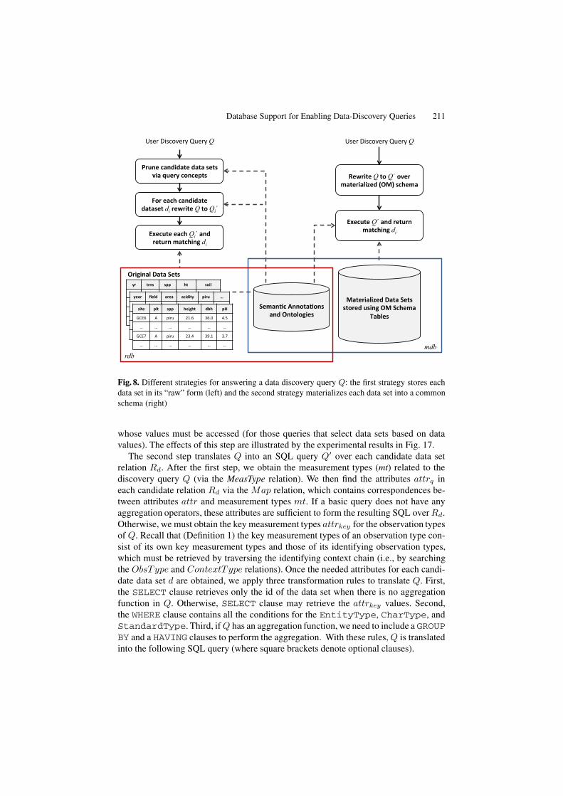
In this section we describe two different strategies for evaluating data discovery queriesover annotated observational data sets. As shown in Fig. 8, both strategies utilize se-mantic annotations (and corresponding ontologies) to answer discovery queries. We as-sume annotations are stored using the relations described in Sect. 2, namely the Annot,ObsType, MeasType, ContextType, and Map tables. The two approaches differ in howthey utilize different representations of the underlying data sets. The first query strategy(rdb) stores each data set in its “raw” form (i.e., “in place”) according to its definedschema. Thus, each data set is stored as a distinct relation in the database. For instance,both data sets of Fig. 1 are stored as tables without any changes to their schemas. Thesecond query strategy (mdb) materializes each data set using the MaterializeDB algo-rithm. In this approach, the observations and measurements stored in each data set arerepresented using the Entity, Obs, Meas, and Context tables described in Sect. 2.1.
In what follows, we first present our approaches for evaluating basic discovery queriesusing these strategies (Subsections 3.1 and 3.2, respectively). Then, in Subsection 3.3we extend these strategies for evaluating complex discovery queries.
3.1 Query Evaluation over In-place Database
Evaluating a basic discovery query Q in the rdb approach consists of three steps. Herewe assume that each data set (denoted by id d) is stored in a relation Rd. The firststep prunes the search space of candidate data sets to select only those data sets withthe required entity, characteristic, and standard types specified within Q. The candidatedata sets (i.e., those that potentially match Q) are selected by accessing the semantic-annotation relations ObsType, MeasType, and Annot. This pruning step can helpdecrease the cost of evaluating discovery queries by reducing the number of data sets
Database Support for Enabling Data-Discovery Queries 211
!"#$%&'"()*#$+%,-#$+%Q !"#$%&'"()*#$+%,-#$+%Q
!" #"$% %&& '# %()*
. . . .
. . . .
. . . .
. . . .
!+,"- .+*/- ,"+,- ,0)/)#!- &)"1- 2-
%)#+ &*# %&& '+)3'# /4' &5
/012 3 4'$- 5672 8279 :7;
. . . . . .
/01< 3 4'$- 587: 8=76 87<
. . . . . .
6,#+"),*)7+/-8,#,-9+#%-%#("+/-1%)$3-:6-90'+;,-
<,4*+%-
:")3)$,*-8,#,-9+#%-
="1$+-0,$/)/,#+-/,#,-%+#%-->),-?1+"!-0($0+&#%-
@("-+,0'-0,$/)/,#+-/,#,%+#-di "+A")#+-Q-#(-Qi´
BC+01#+-+,0'-Qi´-,$/-"+#1"$-;,#0')$3-di-
9+;,$D0-E$$(#,D($%-,$/-:$#(*(3)+%-
F+A")#+-Q-#(-Q´ (>+"-;,#+"),*)7+/-G:6H-%0'+;,
BC+01#+-Q´-,$/-"+#1"$-;,#0')$3-di-
mdb rdb
Fig. 8. Different strategies for answering a data discovery query Q: the first strategy stores eachdata set in its “raw” form (left) and the second strategy materializes each data set into a commonschema (right)
whose values must be accessed (for those queries that select data sets based on datavalues). The effects of this step are illustrated by the experimental results in Fig. 17.
The second step translates Q into an SQL query Q! over each candidate data setrelation Rd. After the first step, we obtain the measurement types (mt) related to thediscovery query Q (via the MeasType relation). We then find the attributes attrq ineach candidate relation Rd via the Map relation, which contains correspondences be-tween attributes attr and measurement types mt. If a basic query does not have anyaggregation operators, these attributes are sufficient to form the resulting SQL over Rd.Otherwise, we must obtain the key measurement types attrkey for the observation typesof Q. Recall that (Definition 1) the key measurement types of an observation type con-sist of its own key measurement types and those of its identifying observation types,which must be retrieved by traversing the identifying context chain (i.e., by searchingthe ObsType and ContextT ype relations). Once the needed attributes for each candi-date data set d are obtained, we apply three transformation rules to translate Q. First,the SELECT clause retrieves only the id of the data set when there is no aggregationfunction in Q. Otherwise, SELECT clause may retrieve the attrkey values. Second,the WHERE clause contains all the conditions for the EntityType, CharType, andStandardType. Third, if Q has an aggregation function, we need to include a GROUPBY and a HAVING clauses to perform the aggregation. With these rules, Q is translatedinto the following SQL query (where square brackets denote optional clauses).
212 H. Cao, S. Bowers, and M.P. Schildhauer
SELECT DISTINCT d[, attrkey ] FROM Rd
WHERE non-aggregation conditions[GROUP BY attrkey ][HAVING aggregation condition];
The third step executes the SQL query over the database after transforming Q to SQLquery Q!.
Example 4. We illustrate the rewriting process with the following example. Considerthe semantic annotations in Fig. 3 and the basic discovery query
Tree(TaxonName = ‘piru’ $ count(distinct !) * 5)
from Subsection 2.2. The first step finds the attributes involved in the condition (i.e.,TaxonName = ‘piru’). From the entity type “Tree” and the characteristic “TaxonName”,we can find the corresponding observation type “ot4”, measurement type “mt5”, andthe attribute “spp”. We then find the key attributes to perform the aggregation. The keymeasurement types for entity type “Tree”, whose observation type is ot4, come fromot4 and ot4’s identifying observation types ot2 and ot1. Since these observation types’key measurement types are mt5, mt3, mt2 and mt1, the key attributes attrkey are spp,size, plt, and site (from the Map relation). The resulting SQL query is expressed asfollows where the data set id is d1 and the corresponding relation is denoted as Rd1.
SELECT DISTINCT d1 FROM Rd1
WHERE spp = ’piru’GROUP BY d1, spp, size, plt, siteHAVING count(*) * 5;
Finally, in the third step of the rdb approach, we execute the SQL query for each of thecandidate data sets such that the answer for Q is the union of these results.
Cost Analysis. The major computation cost using the rdb approach is to send multipleSQL queries to the database server to search the needed information for all the differentcandidate data tables. Given a basic data discovery query Q, it can be translated to |D|Q! queries that must be evaluated over the different data sets in D. Thus, the complexityis O(|D|) where |D| is the total number of data sets in the database. Thus, the costincreases with larger numbers of candidate data sets which we can see from Fig. 21.Note that Q! does not require any join operations, which makes the evaluation of eachQ! efficient.
3.2 Query Evaluation over Materialized Database
The second query strategy (mdb) evaluates a given discovery queryQ over the material-ized database by directly rewriting Q into an SQL query expressed over the annotationand instance relations of Subsection 2.1. This approach differs from rdb, which requiresobtaining the underlying attributes for each individual candidate table and where oneSQL query is constructed per candidate table. Instead, using mdb, a single SQL queryis created to answer the entire basic data discovery query.
Database Support for Enabling Data-Discovery Queries 213
The way in which a basic query is rewritten depends on whether it has an aggre-gation condition. For a basic query without an aggregation condition, we access theEntity and Obs relations to check the entity conditions, and search the MeasType andMeas tables for characteristic and standard conditions. For a basic discovery query withan aggregation condition, we perform the aggregation by grouping Entity.e or Obs.odepending on whether the aggregation is on a distinct entity instance or observation in-stance. Thus, a discovery query Q can be re-written to an SQL query Q! using the mdbapproach as follows.
SELECT DISTINCT Annot.d [, Entity.e][, Obs.o]FROM Annot, Entity, Obs,MeasType,Meas[WHERE table join condition [AND selection condition]][GROUP BY Annot.d[, Entity.e][, Obs.o] ][HAVING aggregation condition ];
where:
table join condition = (Annot.a = MeasType.a)AND (Annot.d = Meas.d) AND (MeasType.mt = Meas.mt)AND (Meas.o = Obs.o) AND (Obs.e = Entity.e)
In this table join condition, there is no need to include the join conditions Meas.d =Obs.d and Obs.d = Entity.d because the observation id Obs.o and the entity idEntity.e are globally unique identifiers. That is, no observation or entity instancesshare the same identifier even though they are from different data sets. If a basic querycontains multiple measurement conditions (of the same entity type), the correspondingSQL query must be combined using “INTERSECTION” or “UNION” operations toanswer the basic query of one entity type.
Example 5. Consider the following query again
Tree(TaxonName = ‘piru’ $ count(distinct !) * 5)
It is rewritten using the mdb approach as:
SELECT DISTINCT Annot.dFROM Annot, Entity, Obs,MeasType,MeasWHERE table join condition
AND MeasType.ct=’TaxonName’ AND Meas.v = ’piru’GROUP BY Annot.d, Obs.oHAVING COUNT(*)>5;
Cost Analysis. The major computation cost in mdb involves the cost of joining over thetype and instance relations, and the selection cost over the measurement values. In mdb,a basic data discovery query Q is translated to only one SQL query Q!. This is moreefficient compared with rdb strategy which translates Q to |D|Q! queries. However, ex-ecuting Q! in mdb involves joining several large instance and type relations. These joinoperations are generally expensive. We do not include the complexity for performingthe join operation because the join strategy is decided by the database system.
214 H. Cao, S. Bowers, and M.P. Schildhauer
Horizontally Partitioned Database. Let the above described mdb approach be de-noted as mdb2 (as opposed to rdb1). Note that mdb2 is a storage scheme consisting ofall the type and instance relations that are described in Sect. 2.1. In the mdb2 storagescheme, the measurement relation Meas contains all the data values in one column,thus these data values share the same data type no matter whether their original datatypes are the same or not. This design of using uniform data type for different datavalues requires utilizing type casting functions provided by the database system to per-form type conversion for evaluating queries with algebraic or aggregation operators.Such type conversion incurs a full scan of the Meas table regardless of whether thereis an index on the value columns or not. Consequently, the query execution over thesimple storage scheme of mdb2 is very costly. To alleviate this issue, we propose topartition the measurement instance table Meas to several horizontally partitioned in-stance tables according to the different data types (e.g., numeric, char, etc.) of the datavalues in their original data sets. The relations coming after partitioning Meas tableare assigned new relation names which start with Meas and have data types as a suf-fix, e.g., MeasNumeric, MeasChar, etc. The new relations are almost the same tothat of Meas(d,m,mt, v, o) with the same attributes except that the data types for thedata value attribute v are different. The partition is done when loading data into thedatabases (i.e., when materializing the data sets). We use mdb3 to denote the storagescheme with the partitioned Meas relations and all the other unpartitioned type and in-stance relations. The mdb3 scheme does not incur additional space overhead comparedwith mdb2 because it stores the same information as Meas, but using several Meas-data-type relations. It can support the same data discovery queries that mdb2 supports.When mdb3 is used to evaluate a data discovery query eQ, the algorithm translates Q toan equivalent SQL expression by replacing all occurrences of Meas to the correspond-ing Meas-data-type relations.
De-Normalized Materialized Database. The join condition shows that a large por-tion of the query evaluation cost comes from the join operation over the measure-ment instance, observation instance, and entity instance relations. To reduce the joincost, we propose to de-normalize multiple relations into a single relation. Consider-ing the most frequently used joins on a basic discovery query, we examine two de-normalization strategies. The first (mdb4) is to de-normalize the Entity, Obs, andMeas relations into a single table to avoid the cost of joining them. The second (mdb5)de-normalization strategy leverages the characteristic type information by also includ-ing (de-normalizing) the MeasType table with the instance tables. The de-normalizedrelation contains the same number of rows as that in Meas although it contains morecolumns than Meas. In the mdb4 scheme, the de-normalized relation contains all theattributes from the Meas relation and three more columns (ot, e, et) from the Obs andEntity relations. That is, it has eight columns (three columns more than that of theoriginal Meas). The new columns in the de-normalized relation may contain duplicatevalues of ot, e, or et. However, the amount of value duplication is generally moder-ate. Thus, mdb4 may still use less space than mdb2 compared with the three instancerelations which contain twelve columns in total. In mdb5, the de-normalized relationcontains all the columns of the de-normalized relation in mdb4, and includes morecolumns (ct, st, · · · ) from the MeasType. These additional columns again contain
Database Support for Enabling Data-Discovery Queries 215
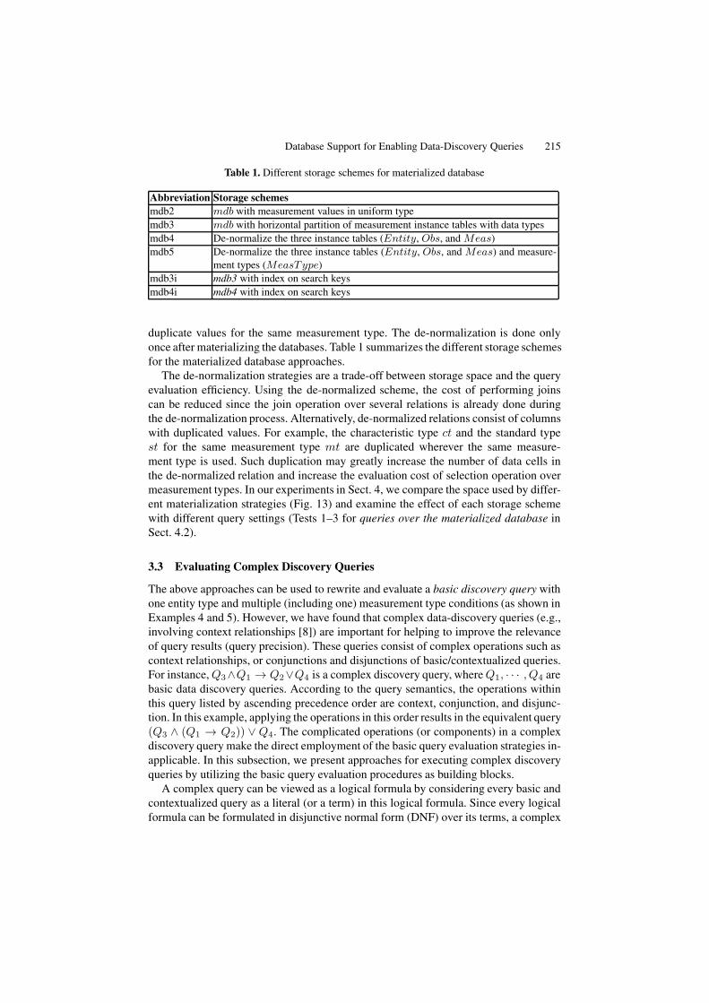
Table 1. Different storage schemes for materialized database
Abbreviation Storage schemesmdb2 mdb with measurement values in uniform typemdb3 mdb with horizontal partition of measurement instance tables with data typesmdb4 De-normalize the three instance tables (Entity, Obs, and Meas)mdb5 De-normalize the three instance tables (Entity, Obs, and Meas) and measure-
ment types (MeasType)mdb3i mdb3 with index on search keysmdb4i mdb4 with index on search keys
duplicate values for the same measurement type. The de-normalization is done onlyonce after materializing the databases. Table 1 summarizes the different storage schemesfor the materialized database approaches.
The de-normalization strategies are a trade-off between storage space and the queryevaluation efficiency. Using the de-normalized scheme, the cost of performing joinscan be reduced since the join operation over several relations is already done duringthe de-normalization process. Alternatively, de-normalized relations consist of columnswith duplicated values. For example, the characteristic type ct and the standard typest for the same measurement type mt are duplicated wherever the same measure-ment type is used. Such duplication may greatly increase the number of data cells inthe de-normalized relation and increase the evaluation cost of selection operation overmeasurement types. In our experiments in Sect. 4, we compare the space used by differ-ent materialization strategies (Fig. 13) and examine the effect of each storage schemewith different query settings (Tests 1–3 for queries over the materialized database inSect. 4.2).
3.3 Evaluating Complex Discovery Queries
The above approaches can be used to rewrite and evaluate a basic discovery query withone entity type and multiple (including one) measurement type conditions (as shown inExamples 4 and 5). However, we have found that complex data-discovery queries (e.g.,involving context relationships [8]) are important for helping to improve the relevanceof query results (query precision). These queries consist of complex operations such ascontext relationships, or conjunctions and disjunctions of basic/contextualized queries.For instance, Q3$Q1 % Q2,Q4 is a complex discovery query, where Q1, · · · , Q4 arebasic data discovery queries. According to the query semantics, the operations withinthis query listed by ascending precedence order are context, conjunction, and disjunc-tion. In this example, applying the operations in this order results in the equivalent query(Q3 $ (Q1 % Q2)) , Q4. The complicated operations (or components) in a complexdiscovery query make the direct employment of the basic query evaluation strategies in-applicable. In this subsection, we present approaches for executing complex discoveryqueries by utilizing the basic query evaluation procedures as building blocks.
A complex query can be viewed as a logical formula by considering every basic andcontextualized query as a literal (or a term) in this logical formula. Since every logicalformula can be formulated in disjunctive normal form (DNF) over its terms, a complex
216 H. Cao, S. Bowers, and M.P. Schildhauer
query can also be converted to a DNF expression. Making use of this property, we canevaluate a complex data-discovery query by converting it into DNF, evaluating eachDNF clause, and merging (through union) the results of all the DNF clauses. Theoreti-cally the conversion of a logical formula to DNF can lead to an exponential explosionof the formula. However, the approach of parsing a query into DNF is still reasonablebecause in practice complex queries generally do not include large numbers of logicalterms.
Each clause in the DNF of a complex query Q is a query block. It is a conjunctivenormal form (CNF) of basic or contextualized discovery queries. In a special situation,a CNF may contain only one basic data discovery query or one contextualized query.For instance, (Q3$(Q1 % Q2)),Q4 has two clauses in its DNF: DNF1 = Q4, whichis a basic query, and the other is DNF2 = Q3 $ (Q1 % Q2), which is the conjunctionof a basic query Q3 and a contextualized query Q1 % Q2.
To evaluate a contextualized queryQC = Q1 % Q2 · · · % Qn, we need to considertwo situations. In the first situation, there is no aggregation condition in any of thebasic query components. In this case, the execution of basic query componentQi is notaffected by any of its context (as described in Subsections 3.1 and 3.2). So, the correctresults of QC can be calculated by evaluating each Qi independently and intersectingtheir results. However, when there is an aggregation condition, to correctly execute thebasic query with the aggregation condition, we need to first apply the conditions in thecontext queries which do not contain any aggregation operator. For instance, given thequery
Tree(max(height) * 20 Meter) % Plot(area < 10 MeterSquared),
the maximum aggregation only applies to trees in a plot with size less than 10m2 asdenoted in Subsection 2.2.
Using this approach, a complex query can be evaluated in two steps.
– Step 1: The first step is to parse a query into its DNF representation. Further, sinceeach DNF clause (a query block) is still complicated when it contains conjunctionsand context, this step further decomposes each DNF clause into basic queries.
– Step 2: In this step, we evaluate and integrate the query blocks by utilizing the querycapacity of a DBMS. For this step, we present two query schemes, ExeD and ExeH.
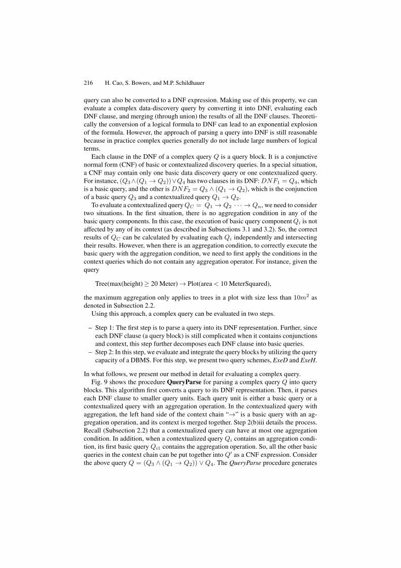
In what follows, we present our method in detail for evaluating a complex query.Fig. 9 shows the procedure QueryParse for parsing a complex query Q into query
blocks. This algorithm first converts a query to its DNF representation. Then, it parseseach DNF clause to smaller query units. Each query unit is either a basic query or acontextualized query with an aggregation operation. In the contextualized query withaggregation, the left hand side of the context chain “%” is a basic query with an ag-gregation operation, and its context is merged together. Step 2(b)iii details the process.Recall (Subsection 2.2) that a contextualized query can have at most one aggregationcondition. In addition, when a contextualized query Qi contains an aggregation condi-tion, its first basic query Qi1 contains the aggregation operation. So, all the other basicqueries in the context chain can be put together into Q! as a CNF expression. Considerthe above query Q = (Q3 $ (Q1 % Q2)) , Q4. The QueryParse procedure generates
Database Support for Enabling Data-Discovery Queries 217
Function QueryParse(Q)/* Output: query blocks of Q */
1. Rewrite Q to DNF;2. For (each DNF clause DNFi) /* Decompose each DNF clause*/
(a) QBi = !; /* Query block for DNFi*/(b) For (each clause Qi % DNFi)
/* Each DNFi is a CNF of basic queries and/or contextualized queries*/i. If Qi is a basic query, add Qi to QBi;ii. If Qi is a contextualized query without aggregation
– For each Qij in Qi, add Qij to QBi;iii. If Qi is a contextualized query with aggregation
A. For each Qij (j ( 2) in Qi, add Qij to Q";B. Add Qi1 $ Q" to QBi;
(c) DNF = DNF )QBi;3. return DNF ;
Fig. 9. Function to parse a complex data discovery query Q to its query blocks
DNF = {QB1, QB2} whereQB2 = {Q4}. As toQB1, whenQ1 does not contain anyaggregation operation, QB1 = {Q1, Q2, Q3}. Otherwise, QB1 = {Q1 % Q2, Q3}.The QueryParse procedure rewrites a query Q in the form of QB1 , · · · , QB|DNF |where each query block QBi (1 + i + |DNF |) is in the form of qui1$ · · ·$quij$ · · · .
ExeD: Executing a Query Based on Decomposed Query Units. ExeD is the firstquery scheme to process a complex query. It executes a query by evaluating its mostdecomposed query units. In ExeD, each of the query units of a DNF clause (i.e., queryblocks) are rewritten into SQL queries and executed. The result of each such most de-composed query unit is combined (outside of the DBMS) to obtain the result of everyDNF clause. The detailed process of the ExeD framework is shown in Fig. 10. Thisframework first utilizes the QueryParse function to reformulate the query into a DNFrepresentation such that each DNF clause is a query block. Then, it executes every DNFclause DNFi by evaluating its query units independently. In particular, when a queryunit represents a basic discovery query, the query unit is executed using one of the strate-gies discussed in Subsections 3.1 and 3.2. When a query unit is a contextualized querywith one context in the context chain (Step 3(b)ii), it means that this query has an aggre-gation operation. ExeD first constructs the condition for the “WHERE” clause from allthe constraining queries (i.e., context). Then it adds the constraining “WHERE” clauseto the SQL expression for the basic query with the aggregation condition, where theconstruction of this SQL expression (especially the GROUP BY and HAVING clauses)follows the principles in translating a basic data discovery query in the previous twosections (Sect. 3.1 for rdb and Sect. 3.2 for mdb). Next, the SQL query is evaluatedusing either an in-place database or a materialized database. Finally, the results of thedifferent DNF clauses are unioned together as the final result.
218 H. Cao, S. Bowers, and M.P. Schildhauer
Algorithm ExeD(Q, db)
1. R = !;2. DNF = QueryParse(Q); /* From the given query, get the DNF. */3. For (each DNFi in DNF ) /* Execute every DNF clause and union their results. */
(a) Ri = !;(b) /* Execute every query block in this DNF clause and intersect their results */
For (each query unit qu in the query block of DNFi)i. If qu is a basic query, sql = form a basic query from qu;ii. else, i.e., qu = q $ {cq} is a contextualized query with aggregation,
– Form a WHERE clause from all the conditions in all cqs;– sql = form a basic query sql from q and add the WHERE clause from cq;
iii. Rib = Execute(sql, db);iv. Ri = Ri * Rib;
(c) R = R )Ri;4. Return R;
Fig. 10. Algorithm to execute a complex data discovery query Q over a database db by executinga query block based on its decomposed query units
The ExeD approach may incur unnecessarily repeated scans of the database since itevaluates each query unit using the DBMS and combines the results externally, outsideof the system. For instance, consider the query
Tree(height * 20 Meter) % Plot(area < 10 MeterSquared).
Using the ExeD approach, we must send two basic queries, Tree(height * 20 Meter)and Plot(area < 10 MeterSquared), to the same table.
ExeH: Executing a Query Based on Holistic Sub-Queries. To overcome the problemof repeated scanning of a table in ExeD, we propose a new strategy based on holistic(as opposed to “decomposed”) sub-queries. Here, “holistic” means that the query unitsare combined together (when it is possible) and are evaluated together. Thus, the ideaof ExeH is to form a “holistic” SQL query for all the possible basic query units andto execute this holistic SQL by taking advantage of the optimization capabilities ofthe DBMS. When a complex query does not contain any aggregation operation, it canbe converted to a holistic SQL by translating conjunction to an “AND” condition or an“INTERSECT” clause, and translating disjunction to an “OR” condition or a “UNION”clause. However, not every complex query can be rewritten to one holistic SQL query.Specifically, queries with aggregations must be performed by grouping key measure-ments. When we have discovery queries with multiple aggregation operations (e.g.,in multiple DNFs), the “GROUP BY” attributes for each aggregation may not be thesame. In ExeH, whose framework is shown in Fig. 11, we categorize query blocks intothose with and without aggregations (Step 3). All the query blocks without aggregationconditions are combined and rewritten to one holistic SQL query (Step 4 to 6), whilethe query blocks with aggregations are processed individually (Step 7). ExeH is verysimilar to ExeD except that it separates the basic queries with aggregations DNFag
and without aggregations DNFnag. For queries without aggregations, we can form a
Database Support for Enabling Data-Discovery Queries 219
Algorithm ExeH(Q, db)
1. R = !;2. DNF = QueryParse(Q); /* From the given query, get the DNF. */3. DNFag , DNFnag = PartitionDNF(DNF );
/* Execute the DNFs without aggregation */4. sql = FormHolisticSql(DNFnag, db);5. Rnag = Execute(sql, db);6. R = R )Rnag
/* Execute every DNF with aggregation */7. For each DNFi in DNFag
(a) sql = construct an SQL statement for DNFi;(b) Rag = Execute(sql, db);(c) R = R )Rag;
8. Return R;
Fig. 11. Algorithm to execute a complex data discovery query Q over a database db by usingholistic query units
holistic SQL (Step 4). For queries with aggregation, we can form SQL statements asStep 3(b)ii in ExeD and execute them.
4 Experimental Evaluation
In this section we describe our experimental results of the framework and the algo-rithms discussed above to evaluate the performance and the scalability (with respect totime and space) of the different query strategies. Our implementation was written inJava, and all experiments were run using an iMac with a 2.66G Intel processor and 4Gvirtual memory. We used PostgreSQL 8.4 as the back-end database system. To reportstable results, all numbers in our figures represent the average result of 10 different runs(materialization tasks or queries) with the same settings for each case.
Data. We generated synthetic data to simulate a number of real data sets used withinthe Santa Barbara Coastal (SBC) Long Term Ecological Research (LTER) project [4].This repository contains -130 data sets where each one has 1K to 10K rows and onaverage 15 to 20 columns. To simulate this repository (to test scalability, etc.), ourdata generator used the following parameters. The average number of attributes andrecords in a data set was 20 and 5K, respectively. The average number of characteristicsfor an entity was two. The distinctive factor f # (0, 1], which represents the ratioof distinct entity/observation instances in a data set, was set to 0.5. We also set thelongest length of context chains to be 5 to test the execution of complex queries withcontext and aggregation. In this way, a data set can have observations with many contextrelationships as well as observations without any context.
Our synthetic data generator also controls attribute selectivity to facilitate the testof query selectivity. In particular, given a selectivity s # (0, 1] of an attribute attr, a
220 H. Cao, S. Bowers, and M.P. Schildhauer
Time (s) vs. num. of rows
0.1
1
10
100
1000
0.5 1 2 5 10 20Number of rows in a dataset (*K)
Tim
e (
s)
No key constraint Key constraint yes context (5)
Instance num, vs. key constraints(Number of data cells 20K)
0
5
10
15
20
25
|EI| |OI| |MI| |CI|
Nu
mb
er
of
inst
an
ces
(*K
)
No key constraintKey constraint yesContext (5)
(a) Time (b) Space
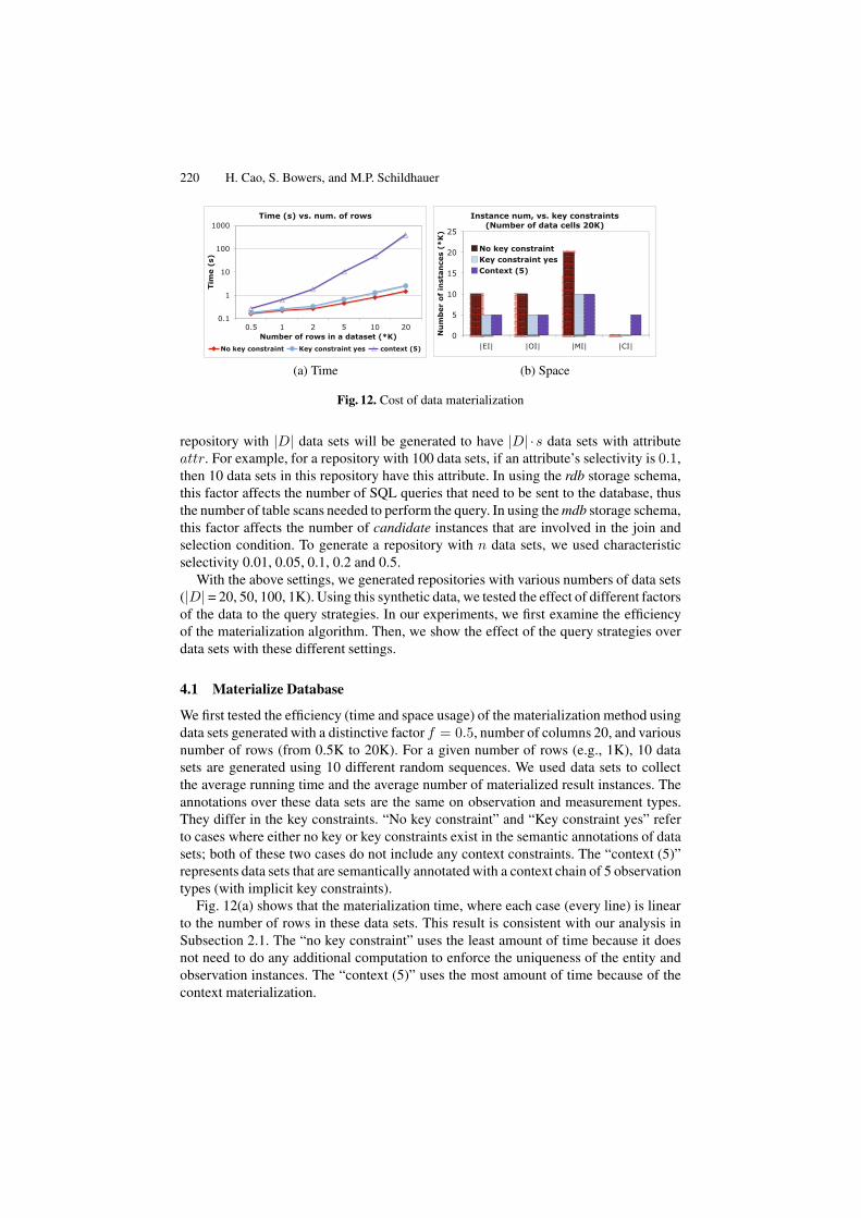
Fig. 12. Cost of data materialization
repository with |D| data sets will be generated to have |D| ·s data sets with attributeattr. For example, for a repository with 100 data sets, if an attribute’s selectivity is 0.1,then 10 data sets in this repository have this attribute. In using the rdb storage schema,this factor affects the number of SQL queries that need to be sent to the database, thusthe number of table scans needed to perform the query. In using the mdb storage schema,this factor affects the number of candidate instances that are involved in the join andselection condition. To generate a repository with n data sets, we used characteristicselectivity 0.01, 0.05, 0.1, 0.2 and 0.5.
With the above settings, we generated repositories with various numbers of data sets(|D| = 20, 50, 100, 1K). Using this synthetic data, we tested the effect of different factorsof the data to the query strategies. In our experiments, we first examine the efficiencyof the materialization algorithm. Then, we show the effect of the query strategies overdata sets with these different settings.
4.1 Materialize Database
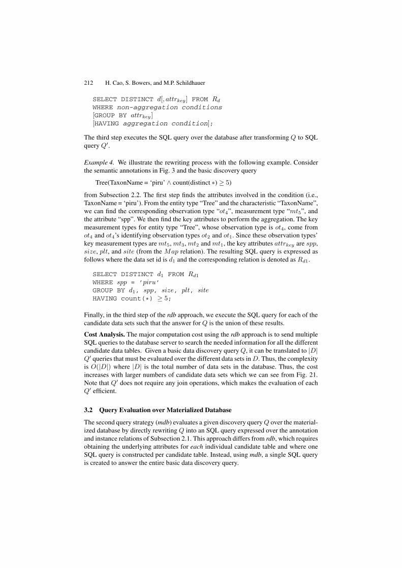
We first tested the efficiency (time and space usage) of the materialization method usingdata sets generated with a distinctive factor f = 0.5, number of columns 20, and variousnumber of rows (from 0.5K to 20K). For a given number of rows (e.g., 1K), 10 datasets are generated using 10 different random sequences. We used data sets to collectthe average running time and the average number of materialized result instances. Theannotations over these data sets are the same on observation and measurement types.They differ in the key constraints. “No key constraint” and “Key constraint yes” referto cases where either no key or key constraints exist in the semantic annotations of datasets; both of these two cases do not include any context constraints. The “context (5)”represents data sets that are semantically annotated with a context chain of 5 observationtypes (with implicit key constraints).
Fig. 12(a) shows that the materialization time, where each case (every line) is linearto the number of rows in these data sets. This result is consistent with our analysis inSubsection 2.1. The “no key constraint” uses the least amount of time because it doesnot need to do any additional computation to enforce the uniqueness of the entity andobservation instances. The “context (5)” uses the most amount of time because of thecontext materialization.
Database Support for Enabling Data-Discovery Queries 221
!"#!!"$!!!"$#!!"%!!!"%#!!"&!!!"&#!!"'!!!"'#!!"
!(#" $" %" #" $!" %!"
!"#
$%&'(
)'*+,+'-%../'01
23'
4'0123'
!"#$%&'()'*+,+'-%../'5/6'#+,%&7+.78+9(4'/,&+,%:;')*+%")*+&")*+'")*+#"
Fig. 13. Space complexity of different data materialization strategies
Fig. 12(b) plots the number of instances generated for a data set with 20K data cells.For the case without any key constraints, the number of measurement instances is thesame as the number of data cells because it treats every cell as a different instance,even though different cells may carry the same value. However, for the case with keyconstraints, half the number of instances are used since the distinctive factor f is 0.5.When the context chain is of length 5, the number of context instances is the number ofobservation instances times the chain length.
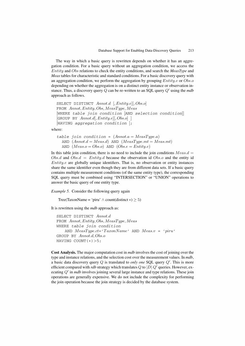
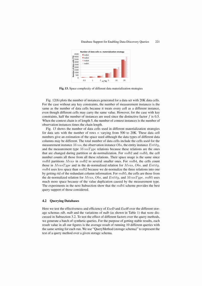
Fig. 13 shows the number of data cells used in different materialization strategiesfor data sets with the number of rows n varying from 500 to 20K. These data cellnumbers give an estimation of the space used although the data types of different datacolumns may be different. The total number of data cells include the cells used for themeasurement instance Meas, the observation instance Obs, the entity instance Entity,and the measurement type MeasType relations because these relations are the onesthat are changed during partition or de-normalization. For mdb2 and mdb3, the cellnumber counts all those from all these relations. Their space usage is the same sincemdb3 partitions Meas in mdb2 to several smaller ones. For mdb4, the cells countthose in MeasType and in the de-normalized relation for Meas, Obs, and Entity.mdb4 uses less space than mdb2 because we de-normalize the three relations into oneby getting rid of the redundant column information. For mdb5, the cells are those fromthe de-normalized relation for Meas, Obs, and Entity, and MeasType. mdb5 usesmuch more space because of the value duplication caused by the measurement type.The experiments in the next Subsection show that the mdb4 scheme provides the bestquery support of those considered.
4.2 Querying Databases
Here we test the effectiveness and efficiency of ExeD and ExeH over the different stor-age schemas rdb, mdb and the variations of mdb (as shown in Table 1) that were dis-cussed in Subsection 3.2. To test the effect of different factors over the query methods,we generate a batch of synthetic queries. For the purpose of getting stable results, eachresult value in all our figures is the average result of running 10 different queries withthe same setting for each run. We use “QueryMethod (storage schema)” to represent thetest of a query method over a given storage schema.
222 H. Cao, S. Bowers, and M.P. Schildhauer
The synthetic query generator generates three different types of queries to test thefeasibility of the query strategies. These include queries with different numbers of logicconnectors (e.g., AND, OR), with different lengths of context chains, and with aggre-gation functions.
To test the effect of the different approaches over the storage schema, the query gen-erator controls the query selectivity by using the characteristic selectivity and valueselectivity. Characteristic selectivity corresponds to the attribute selectivity in the syn-thetic data generator. To generate a query with a given characteristic selectivity, we sim-ply retrieve the corresponding attributes that have this selectivity. The value selectivitysval (# (0, 1]) determines the percentage of data rows in a data set that satisfy a givenmeasurement condition. For example, when the selection condition mval * 10.34 forcharacteristic “Height” has value selectivity 0.1, then a table with 1K records has 100rows satisfying this selection condition. Thus, this factor controls the number of resultinstances of a query. To generate a query condition satisfying a value selectivity, wefirst count the number of distinctive values (or value combinations) for an attribute (orattributes). We then combine them to create conditions with a given selectivity. The syn-thetic queries are generated with different characteristic selectivities. For data sets withthe same characteristic selectivity, we generated queries with value selectivity 0.001,0.01, 0.1, 0.2 and 0.5.
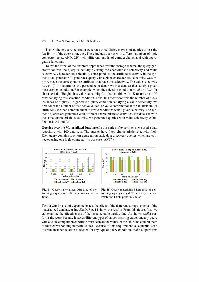
Queries over the Materialized Database. In this series of experiments, we used a datarepository with 100 data sets. The queries have fixed characteristic selectivity 0.01.Each query contains two non-aggregation basic data-discovery queries which are con-nected using one logic connector (in our case “AND”).
Time vs. ExeD(mdb*) vs. val. sel. (cha. Sel. = 0.01)
0
10
20
30
40
50
0.001 0.01 0.1 0.2 0.5Value selectivity
Tim
e (
s)
ExeD(mdb2) ExeD(mdb3)ExeD(mdb4) ExeD(mdb5)
Fig. 14. Query materialized DB: time of per-forming a query over different storage varia-tions.
Time vs. ExeD(mdb) vs. ExeH(mdb) (cha. sel. = 0.01)
0
2
4
6
8
10
0.001 0.01 0.1 0.2 0.5Value selectivity
Tim
e (
s)
ExeD(mdb3) ExeD(mdb4)ExeH(mdb3) ExeH(mdb4)
Fig. 15. Query materialized DB: time of per-forming a query using different query strategy:ExeD and ExeH perform similar
Test 1: Our first set of experiments test the effect of the different storage schema of thematerialized database using ExeD. Fig. 14 shows the results. From this figure, first, wecan examine the effectiveness of the instance table partitioning. As shown, mdb2 per-forms the worst because it stores different types of values as string values and any querywith a value comparison condition must scan all the values of the table and convert themto their corresponding numeric values. Because of this requirement, a sequential scanover the instance relation is needed for any type of query condition. mdb3 outperforms
Database Support for Enabling Data-Discovery Queries 223
Time vs. ExeD(mdb vs. mdbi) (cha. sel. = 0.01)
0.01
0.1
1
10
0.001 0.01 0.1 0.2 0.5
Value selectivity
Tim
e (
s)
ExeD(mdb3) ExeD(mdb4)ExeD(mdb3i) ExeD(mdb4i)
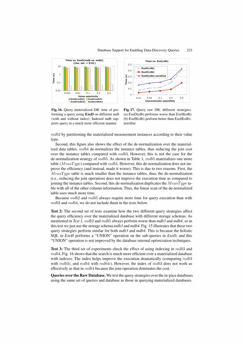
Fig. 16. Query materialized DB: time of per-forming a query using ExeD on different mdb(with and without index): Indexed mdb sup-ports query in a much more efficient manner
Time vs. Exe(rdb)
0
0.1
0.2
0.3
0.4
0.5
0.01 0.05 0.1 0.2 0.5Characteristic selectibity
Tim
e (
s)
ExeD(rdb)
ExeH(rdb)
ExeH(rdb)-norefine
Fig. 17. Query raw DB: different strategies:(a) ExeD(rdb) performs worse than ExeH(rdb)(b) ExeH(rdb) perform better than ExeH(rdb)-norefine
mdb2 by partitioning the materialized measurement instances according to their valuetype.
Second, this figure also shows the effect of the de-normalization over the material-ized data tables. mdb4 de-normalizes the instance tables, thus reducing the join costover the instance tables compared with mdb3. However, this is not the case for thede-normalization strategy of mdb5. As shown in Table 1, mdb5 materializes one moretable (MeasType) compared with mdb4. However, this de-normalization does not im-prove the efficiency (and instead, made it worse). This is due to two reasons. First, theMeasType table is much smaller than the instance tables, thus, the de-normalization(i.e., reducing the join operation) does not improve the execution time as compared tojoining the instance tables. Second, this de-normalization duplicates the MeasType ta-ble with all of the other column information. Thus, the linear scan of the de-normalizedtable uses much more time.
Because mdb2 and mdb5 always require more time for query execution than withmdb3 and mdb4, we do not include them in the tests below.
Test 2: The second set of tests examine how the two different query strategies affectthe query efficiency over the materialized database with different storage schemas. Asmentioned in Test 1, mdb2 and mdb5 always perform worse than mdb3 and mdb4, so inthis test we just use the storage schema mdb3 and mdb4. Fig. 15 illustrates that these twoquery strategies perform similar for both mdb3 and mdb4. This is because the holisticSQL in ExeH performs a “UNION” operation on the sub-queries in ExeD, and this“UNION” operation is not improved by the database internal optimization techniques.
Test 3: The third set of experiments check the effect of using indexing in mdb3 andmdb4. Fig. 16 shows that the search is much more efficient over a materialized databasewith indexes. The index helps improve the execution dramatically (comparing mdb3with mdb3i, and mdb4 with mdb4i). However, the index of mdb3 does not work aseffectively as that in mdb4 because the join operation dominates the cost.
Queries over the Raw Database. We test the query strategies over the in-pace databasesusing the same set of queries and database as those in querying materialized databases.
224 H. Cao, S. Bowers, and M.P. Schildhauer
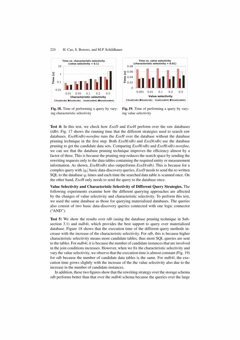
Time vs. characteristic selectivity (value selectivity = 0.1)
0.01
0.1
1
10
0.01 0.05 0.1 0.2 0.5Characteristic selectivity
Tim
e (
s)
ExeD(rdb) ExeH(rdb) ExeD(mdb4i) ExeH(mdb4i)
Fig. 18. Time of performing a query by vary-ing characteristic selectivity
Time vs. value selectivity (characteristic selectivity = 0.01)
0
0.02
0.04
0.06
0.08
0.001 0.01 0.1 0.2 0.5
Value selectivity
Tim
e (
s)
ExeD(rdb) ExeH(rdb) ExeD(mdb4i) ExeH(mdb4i)
Fig. 19. Time of performing a query by vary-ing value selectivity
Test 4: In this test, we check how ExeD and ExeH perform over the raw databases(rdb). Fig. 17 shows the running time that the different strategies used to search rawdatabases. ExeH(rdb)-norefine runs the ExeH over the database without the databasepruning technique in the first step. Both ExeH(rdb) and ExeD(rdb) use the databasepruning to get the candidate data sets. Comparing ExeH(rdb) and ExeH(rdb)-norefine,we can see that the database pruning technique improves the efficiency almost by afactor of three. This is because the pruning step reduces the search space by sending therewriting requests only to the data tables containing the required entity or measurementinformation. As shown, ExeH(rdb) also outperforms ExeD(rdb). This is because for acomplex query with |qb| basic data-discovery queries, ExeD needs to send the re-writtenSQL to the database qb times and each time the searched data table is scanned once. Onthe other hand, ExeH only needs to send the query to the database once.
Value Selectivity and Characteristic Selectivity of Different Query Strategies. Thefollowing experiments examine how the different querying approaches are affectedby the changes of value selectivity and characteristic selectivity. To perform this test,we used the same database as those for querying materialized databases. The queriesalso consist of two basic data-discovery queries connected with one logic connector(“AND”).
Test 5: We show the results over rdb (using the database pruning technique in Sub-section 3.1) and mdb4i, which provides the best support to query over materializeddatabase. Figure 18 shows that the execution time of the different query methods in-crease with the increase of the characteristic selectivity. For rdb, this is because highercharacteristic selectivity means more candidate tables, thus more SQL queries are sentto the tables. For mdb4i, it is because the number of candidate instances that are involvedin the join conditions increases. However, when we fix the characteristic selectivity andvary the value selectivity, we observe that the execution time is almost constant (Fig. 19)for rdb because the number of candidate data tables is the same. For mdb4i, the exe-cution time grows slightly with the increase of the the value selectivity also due to theincrease in the number of candidate instances.
In addition, these two figures show that the rewriting strategy over the storage schemardb performs better than that over the mdb4i schema because the queries over the large
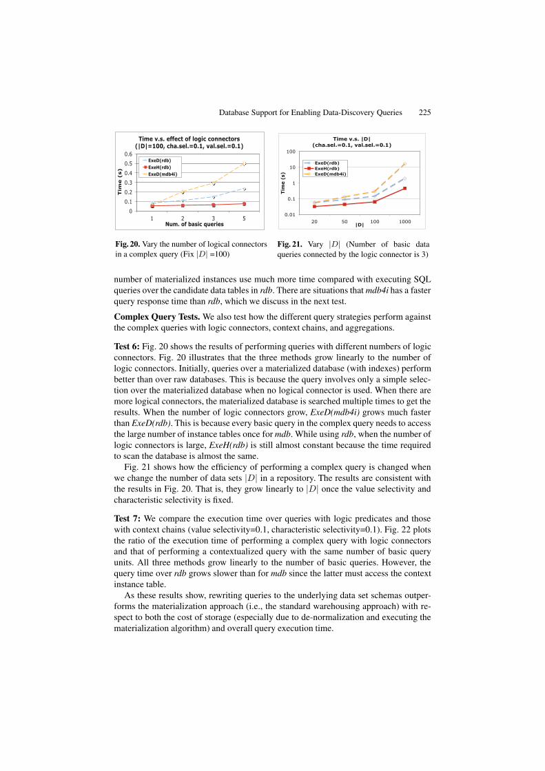
Database Support for Enabling Data-Discovery Queries 225
0
0.1
0.2
0.3
0.4
0.5
0.6
1 2 3 5
Tim
e (
s)
Num. of basic queries
Time v.s. effect of logic connectors (|D|=100, cha.sel.=0.1, val.sel.=0.1)
ExeD(rdb) ExeH(rdb) ExeD(mdb4i)
Fig. 20. Vary the number of logical connectorsin a complex query (Fix |D| =100)
Time v.s. |D|(cha.sel.=0.1, val.sel.=0.1)
0.01
0.1
1
10
100
20 50 100 1000|D|
Tim
e (
s)
ExeD(rdb)ExeH(rdb)ExeD(mdb4i)
Fig. 21. Vary |D| (Number of basic dataqueries connected by the logic connector is 3)
number of materialized instances use much more time compared with executing SQLqueries over the candidate data tables in rdb. There are situations that mdb4i has a fasterquery response time than rdb, which we discuss in the next test.
Complex Query Tests. We also test how the different query strategies perform againstthe complex queries with logic connectors, context chains, and aggregations.
Test 6: Fig. 20 shows the results of performing queries with different numbers of logicconnectors. Fig. 20 illustrates that the three methods grow linearly to the number oflogic connectors. Initially, queries over a materialized database (with indexes) performbetter than over raw databases. This is because the query involves only a simple selec-tion over the materialized database when no logical connector is used. When there aremore logical connectors, the materialized database is searched multiple times to get theresults. When the number of logic connectors grow, ExeD(mdb4i) grows much fasterthan ExeD(rdb). This is because every basic query in the complex query needs to accessthe large number of instance tables once for mdb. While using rdb, when the number oflogic connectors is large, ExeH(rdb) is still almost constant because the time requiredto scan the database is almost the same.
Fig. 21 shows how the efficiency of performing a complex query is changed whenwe change the number of data sets |D| in a repository. The results are consistent withthe results in Fig. 20. That is, they grow linearly to |D| once the value selectivity andcharacteristic selectivity is fixed.
Test 7: We compare the execution time over queries with logic predicates and thosewith context chains (value selectivity=0.1, characteristic selectivity=0.1). Fig. 22 plotsthe ratio of the execution time of performing a complex query with logic connectorsand that of performing a contextualized query with the same number of basic queryunits. All three methods grow linearly to the number of basic queries. However, thequery time over rdb grows slower than for mdb since the latter must access the contextinstance table.
As these results show, rewriting queries to the underlying data set schemas outper-forms the materialization approach (i.e., the standard warehousing approach) with re-spect to both the cost of storage (especially due to de-normalization and executing thematerialization algorithm) and overall query execution time.
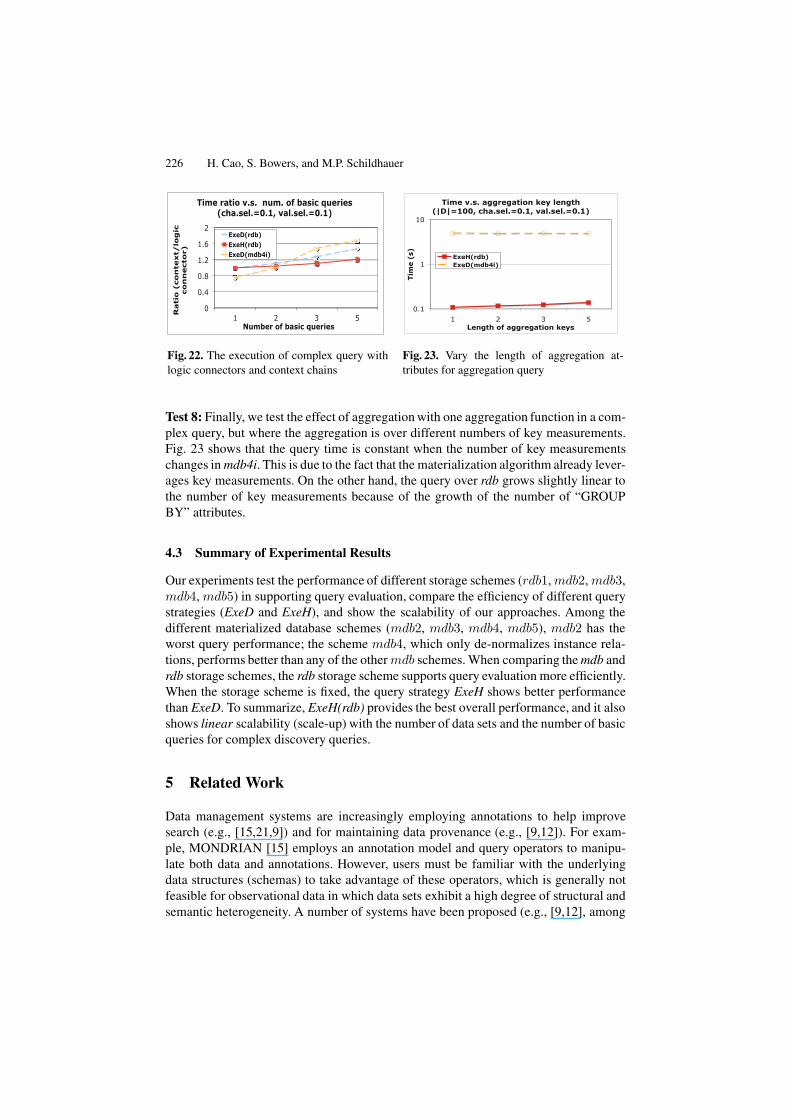
226 H. Cao, S. Bowers, and M.P. Schildhauer
0
0.4
0.8
1.2
1.6
2
1 2 3 5
Rati
o (
co
nte
xt/
log
ic
co
nn
ecto
r)
Number of basic queries
Time ratio v.s. num. of basic queries (cha.sel.=0.1, val.sel.=0.1)
ExeD(rdb) ExeH(rdb) ExeD(mdb4i)
Fig. 22. The execution of complex query withlogic connectors and context chains
Time v.s. aggregation key length(|D|=100, cha.sel.=0.1, val.sel.=0.1)
0.1
1
10
1 2 3 5Length of aggregation keys
Tim
e (
s) ExeH(rdb)ExeD(mdb4i)
Fig. 23. Vary the length of aggregation at-tributes for aggregation query
Test 8: Finally, we test the effect of aggregation with one aggregation function in a com-plex query, but where the aggregation is over different numbers of key measurements.Fig. 23 shows that the query time is constant when the number of key measurementschanges in mdb4i. This is due to the fact that the materialization algorithm already lever-ages key measurements. On the other hand, the query over rdb grows slightly linear tothe number of key measurements because of the growth of the number of “GROUPBY” attributes.
4.3 Summary of Experimental Results
Our experiments test the performance of different storage schemes (rdb1, mdb2, mdb3,mdb4, mdb5) in supporting query evaluation, compare the efficiency of different querystrategies (ExeD and ExeH), and show the scalability of our approaches. Among thedifferent materialized database schemes (mdb2, mdb3, mdb4, mdb5), mdb2 has theworst query performance; the scheme mdb4, which only de-normalizes instance rela-tions, performs better than any of the other mdb schemes. When comparing the mdb andrdb storage schemes, the rdb storage scheme supports query evaluation more efficiently.When the storage scheme is fixed, the query strategy ExeH shows better performancethan ExeD. To summarize, ExeH(rdb) provides the best overall performance, and it alsoshows linear scalability (scale-up) with the number of data sets and the number of basicqueries for complex discovery queries.
5 Related Work
Data management systems are increasingly employing annotations to help improvesearch (e.g., [15,21,9]) and for maintaining data provenance (e.g., [9,12]). For exam-ple, MONDRIAN [15] employs an annotation model and query operators to manipu-late both data and annotations. However, users must be familiar with the underlyingdata structures (schemas) to take advantage of these operators, which is generally notfeasible for observational data in which data sets exhibit a high degree of structural andsemantic heterogeneity. A number of systems have been proposed (e.g., [9,12], among

Database Support for Enabling Data-Discovery Queries 227
others) for propagating annotations (as simple text attached to data) through queries aswell as for providing the ability to query over annotations. Efforts have also been carriedout for leveraging annotations, e.g., for the discovery of domain-specific data [16,23].These approaches are largely based on keyword queries, and do not consider structuredsearches. Our work differs from these approaches in that we consider a highly struc-tured and generic model for annotations with the aim of providing a uniform approachfor issuing structured data-discovery searches.
Our work is closely aligned to traditional data integration approaches (e.g., [17,19]),where a global mediated schema is used to (physically or logically) merge the structuresof heterogeneous data sources using mapping constraints among the source and targetschemas. As such, the observational model we employ in our framework can be viewedas a (general-purpose) mediation schema for observational data sets. This schema canbe augmented with logic rules (as target constraints) and uses the semantic annotationsas mapping constraints. However, instead of users specifying logic constraints directly,we provide a high-level annotation language that simplifies the specification of map-pings and more naturally aligns with the observation model. While it is possible toexpress annotations given in the annotation language as first-order dependencies (e.g.,[7]) together with object creation, our work focuses on exploring and implementingpractical approaches for rewriting and optimizing queries that can include aggregationand summarization operators over our annotation approach.
6 Conclusion
We have presented a novel framework for querying observational data based on formalsemantic annotations to capture the common observational semantic types and theirrelationships and a data discovery language that allows structural queries over bothschema and data. We also have considered different strategies for efficiently implement-ing the framework. We examined the effect of different storage schemes. The in-placescheme rdb stores data tables for each data set; while the materialized scheme mdb ma-terializes the contents in all the data sets into a central warehouse. We also presentedtwo query strategies (ExeD and ExeH) to search semantically annotated data using thedifferent storage schemes. The query strategy ExeD executes a data discovery query bydecomposing it into query units and evaluating each query unit independently. ExeH onthe other hand executes a query by executing its query units in a holistic manner. Ourexperiments show that in most cases answering queries “in place” (rdb) by utilizingExeH outperforms more traditional warehouse-based approaches (using either ExeH orExeD) even after applying different indexing schemes to the warehouse data. As futurework, we intend to develop other query schemes by utilizing a DBMS’s internal statisti-cal information about the data, and to investigate newer parallel-processing approaches(such as MapReduce style distributed processing over key-value data stores) to helpimprove the efficiency and scalability of queries over semantic annotations.
Acknowledgements. We would also like to thank the reviewers for their thoughtfulcomments on the paper as well as Matt Jones, Margaret O’Brien, and Ben Leinfelderfor their contributions to the development and testing of semantic annotation supportwithin Metacat.
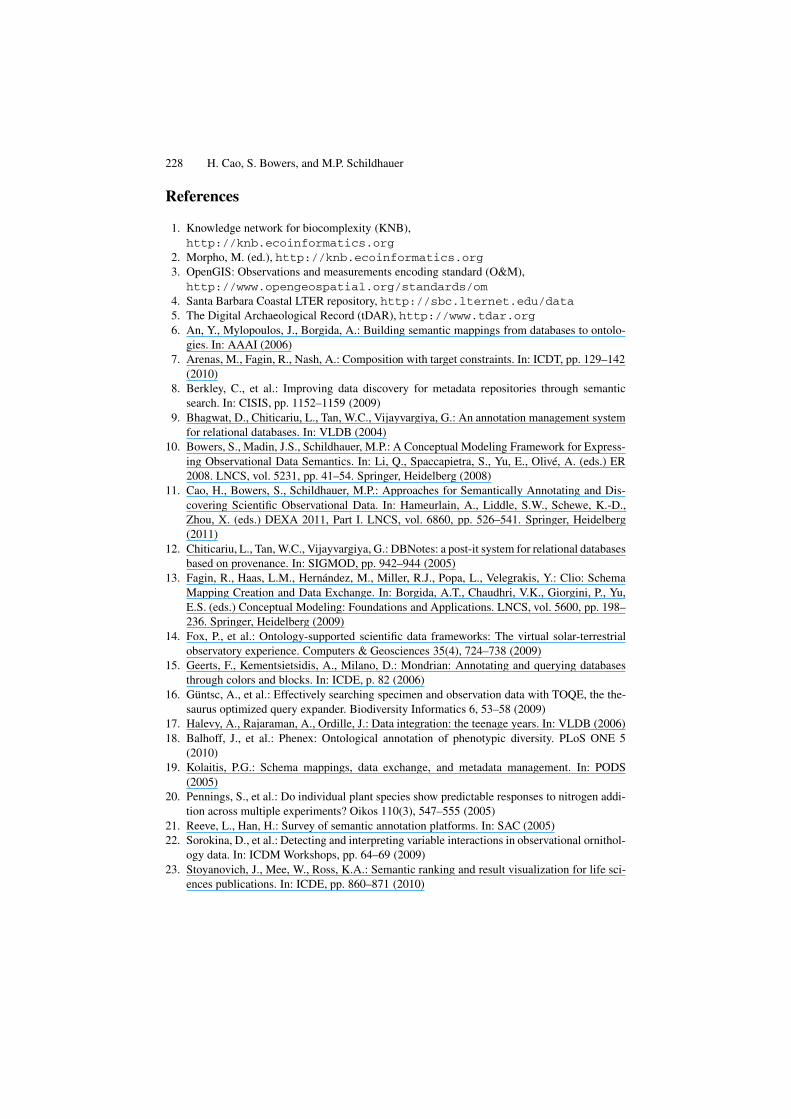
228 H. Cao, S. Bowers, and M.P. Schildhauer
References
1. Knowledge network for biocomplexity (KNB),http://knb.ecoinformatics.org
2. Morpho, M. (ed.), http://knb.ecoinformatics.org3. OpenGIS: Observations and measurements encoding standard (O&M),
http://www.opengeospatial.org/standards/om4. Santa Barbara Coastal LTER repository, http://sbc.lternet.edu/data5. The Digital Archaeological Record (tDAR), http://www.tdar.org6. An, Y., Mylopoulos, J., Borgida, A.: Building semantic mappings from databases to ontolo-
gies. In: AAAI (2006)7. Arenas, M., Fagin, R., Nash, A.: Composition with target constraints. In: ICDT, pp. 129–142
(2010)8. Berkley, C., et al.: Improving data discovery for metadata repositories through semantic
search. In: CISIS, pp. 1152–1159 (2009)9. Bhagwat, D., Chiticariu, L., Tan, W.C., Vijayvargiya, G.: An annotation management system
for relational databases. In: VLDB (2004)10. Bowers, S., Madin, J.S., Schildhauer, M.P.: A Conceptual Modeling Framework for Express-
ing Observational Data Semantics. In: Li, Q., Spaccapietra, S., Yu, E., Olive, A. (eds.) ER2008. LNCS, vol. 5231, pp. 41–54. Springer, Heidelberg (2008)
11. Cao, H., Bowers, S., Schildhauer, M.P.: Approaches for Semantically Annotating and Dis-covering Scientific Observational Data. In: Hameurlain, A., Liddle, S.W., Schewe, K.-D.,Zhou, X. (eds.) DEXA 2011, Part I. LNCS, vol. 6860, pp. 526–541. Springer, Heidelberg(2011)
12. Chiticariu, L., Tan, W.C., Vijayvargiya, G.: DBNotes: a post-it system for relational databasesbased on provenance. In: SIGMOD, pp. 942–944 (2005)
13. Fagin, R., Haas, L.M., Hernandez, M., Miller, R.J., Popa, L., Velegrakis, Y.: Clio: SchemaMapping Creation and Data Exchange. In: Borgida, A.T., Chaudhri, V.K., Giorgini, P., Yu,E.S. (eds.) Conceptual Modeling: Foundations and Applications. LNCS, vol. 5600, pp. 198–236. Springer, Heidelberg (2009)
14. Fox, P., et al.: Ontology-supported scientific data frameworks: The virtual solar-terrestrialobservatory experience. Computers & Geosciences 35(4), 724–738 (2009)
15. Geerts, F., Kementsietsidis, A., Milano, D.: Mondrian: Annotating and querying databasesthrough colors and blocks. In: ICDE, p. 82 (2006)
16. Guntsc, A., et al.: Effectively searching specimen and observation data with TOQE, the the-saurus optimized query expander. Biodiversity Informatics 6, 53–58 (2009)
17. Halevy, A., Rajaraman, A., Ordille, J.: Data integration: the teenage years. In: VLDB (2006)18. Balhoff, J., et al.: Phenex: Ontological annotation of phenotypic diversity. PLoS ONE 5
(2010)19. Kolaitis, P.G.: Schema mappings, data exchange, and metadata management. In: PODS
(2005)20. Pennings, S., et al.: Do individual plant species show predictable responses to nitrogen addi-
tion across multiple experiments? Oikos 110(3), 547–555 (2005)21. Reeve, L., Han, H.: Survey of semantic annotation platforms. In: SAC (2005)22. Sorokina, D., et al.: Detecting and interpreting variable interactions in observational ornithol-
ogy data. In: ICDM Workshops, pp. 64–69 (2009)23. Stoyanovich, J., Mee, W., Ross, K.A.: Semantic ranking and result visualization for life sci-
ences publications. In: ICDE, pp. 860–871 (2010)
Related Documents