Data Visualization The commonality between science and art is in trying to see profoundly - to develop strategies of seeing and showing Edward Tufte.

Data Visualization

The commonality between science and art is in trying to see profoundly - to develop strategies of seeing and

showingEdward Tufte

Visualization skills

Humans are particularly skilled at processing visual informationAn innate capability comparedOur ancestors were those who were efficient visual processors and quickly detected threats and used this information to make effective decisions

A graphical representation of Napoleon Bonaparte's invasion of and subsequent retreat from Russia during 1812. The graph shows the size of the army, its location and the direction of its movement. The temperature during the retreat is drawn at the bottom of figure, which was drawn by Charles Joseph Minard in 1861 and is generally considered to be one of the finest graphs ever produced.

Wilkinson’s grammar of graphics

DataA set of data operations that create variables from datasets

TransVariable transformations

ScaleScale transformations

CoordA coordinate system

ElementGraph and its aesthetic attributes

GuideOne or more guides

ggvis

An implementation of the grammar of graphics in RThe grammar describes the structure of a graphicA graphic is a mapping of data to a visual representationggvis

Data

Spreadsheet approachUse an existing spreadsheet or create a new oneExport as CSV file

DatabaseExecute SQL query

Transformation

A transformation converts data into a format suitable for the intended visualization

# compute a new column in carbon containing the relative change in CO2carbon$relCO2 = (carbon$CO2-280)/280

Coord

A coordinate system describes where things are locatedMost graphs are plotted on a two-dimensional (2D) grid with x (horizontal) and y (vertical) coordinatesThe default coordinate system for most graphic packages is Cartesian.

Element

An element is a graph and its aesthetic attributesBuild a graph by adding layers

library(ggvis)url <- 'http://people.terry.uga.edu/rwatson/data/carbon.txt'carbon <- read.table(url, header=T, sep=',')# Select year(x) and CO2(y) to create a x-y point plot# Specify red points, as you find that aesthetically pleasingcarbon %>% ggvis(~year,~CO2) %>% layer_points(fill:=‘red’)# Notice how ‘%>%’ is used for creating a pipeline of commands

Element

Scalecarbon %>% ggvis(~year,~CO2) %>% layer_points(fill:='red') %>% scale_numeric('y',zero=T)

Axes# Compute a new column containing the relative change in CO2carbon$relCO2 = (carbon$CO2-280)/280carbon %>% ggvis(~year,~relCO2) %>% layer_lines(stroke:='blue') %>% scale_numeric('y',zero=T) %>% add_axis('y', title = "CO2 ppm of the atmosphere", title_offset=50) %>% add_axis('x', title ='Year', format = '####')

Guides

Axes and legends are both forms of guidesHelps the viewer to understand a graphic

Exercise

Create a line plot using the data in the following table.

Year 1804 1927 1960 1974 1987 1999 2012 2027 2046

Population(billions)

1 2 3 4 5 6 7 8 9

Histogramlibrary(ggvis)url <- 'http://people.terry.uga.edu/rwatson/data/centralparktemps.txt't <- read.table(url, header=T, sep=',')t$C <- round((t$temperature - 32)*5/9,1)t %>% ggvis(~C) %>% layer_histograms(width = 2, fill:='cornflowerblue') %>% add_axis('x',title='Celsius') %>% add_axis('y',title='Frequency')

Bar graphlibrary(ggvis)library(RMySQL)conn <- dbConnect(RMySQL::MySQL(), "richardtwatson.com", dbname="ClassicModels", user="db1", password="student")# Query the database and create file for use with Rd <- dbGetQuery(conn,"SELECT productLine from Products;") # Plot the number of product lines by specifying the appropriate column named %>% ggvis(~productLine) %>% layer_bars(fill:='chocolate')add_axis('x',title='Product line') %>% add_axis(‘y’,title='Count')

Exercise

Create a bar graph using the data in the following table

Year 1804 1927 1960 1974 1987 1999 2012 2027 2046

Population(billions)

1 2 3 4 5 6 7 8 9

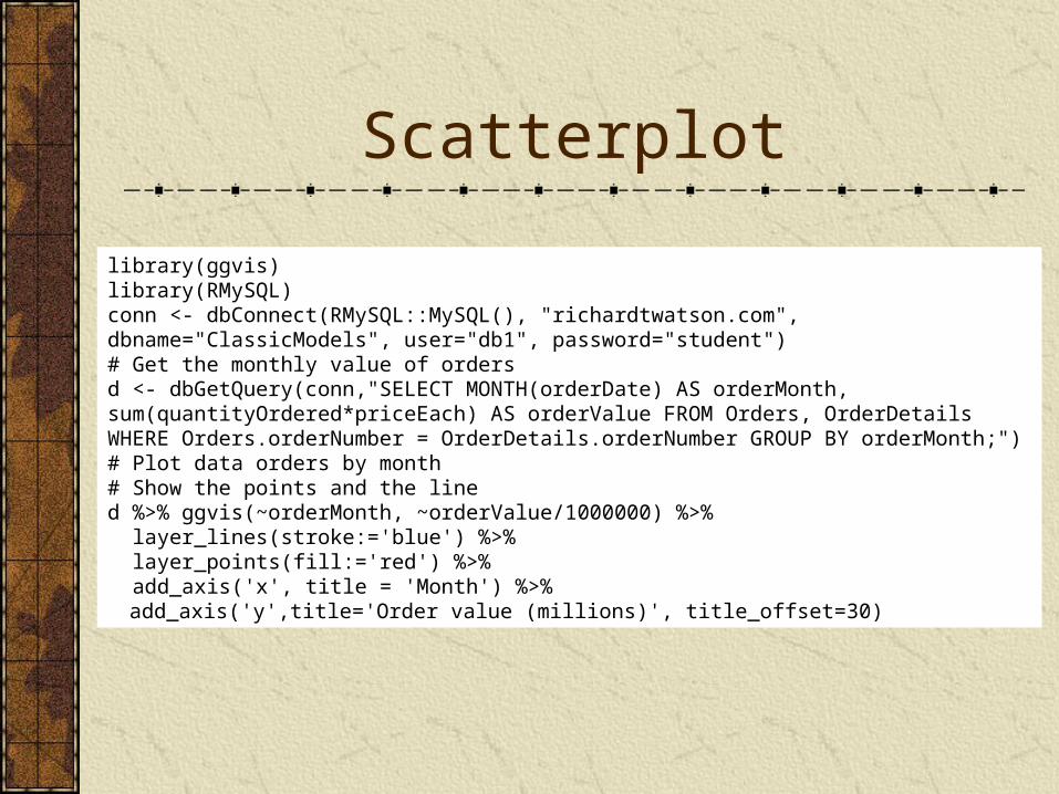
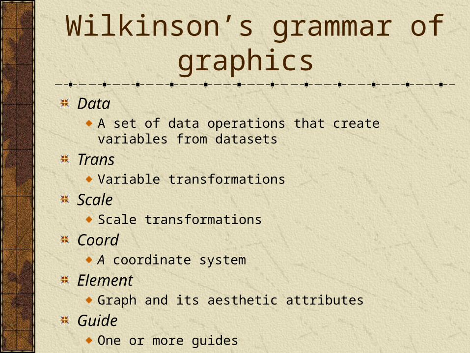
Scatterplot

library(ggvis)library(RMySQL)conn <- dbConnect(RMySQL::MySQL(), "richardtwatson.com", dbname="ClassicModels", user="db1", password="student")# Get the monthly value of ordersd <- dbGetQuery(conn,"SELECT MONTH(orderDate) AS orderMonth, sum(quantityOrdered*priceEach) AS orderValue FROM Orders, OrderDetails WHERE Orders.orderNumber = OrderDetails.orderNumber GROUP BY orderMonth;") # Plot data orders by month# Show the points and the lined %>% ggvis(~orderMonth, ~orderValue/1000000) %>% layer_lines(stroke:='blue') %>% layer_points(fill:='red') %>% add_axis('x', title = 'Month') %>% add_axis('y',title='Order value (millions)', title_offset=30)

Scatterplot

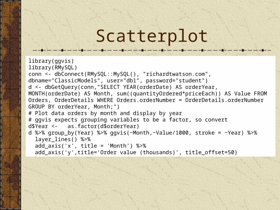
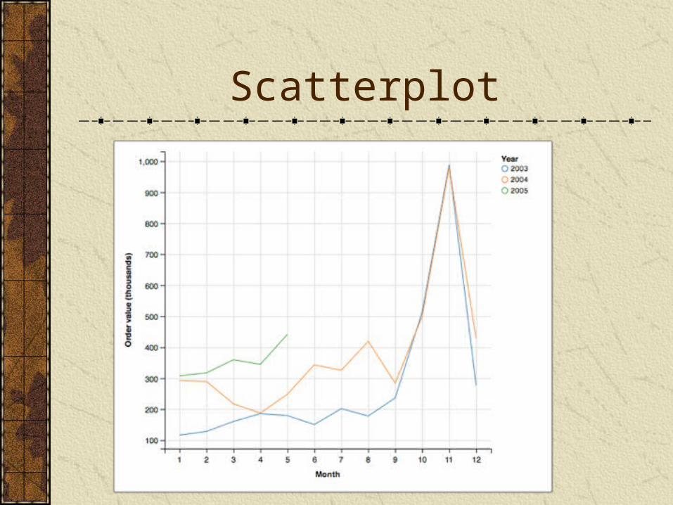
Scatterplotlibrary(ggvis)library(RMySQL)conn <- dbConnect(RMySQL::MySQL(), "richardtwatson.com", dbname="ClassicModels", user="db1", password="student")d <- dbGetQuery(conn,"SELECT YEAR(orderDate) AS orderYear, MONTH(orderDate) AS Month, sum((quantityOrdered*priceEach)) AS Value FROM Orders, OrderDetails WHERE Orders.orderNumber = OrderDetails.orderNumber GROUP BY orderYear, Month;")# Plot data orders by month and display by year# ggvis expects grouping variables to be a factor, so convertd$Year <- as.factor(d$orderYear)d %>% group_by(Year) %>% ggvis(~Month,~Value/1000, stroke = ~Year) %>% layer_lines() %>% add_axis('x', title = 'Month') %>% add_axis('y',title='Order value (thousands)', title_offset=50)

Scatterplot

Bar graphd %>% group_by(Year) %>% ggvis( ~Month, ~Value/100000, fill = ~Year) %>% layer_bars() %>% add_axis('x', title = 'Month') %>% add_axis('y',title='Order value (thousands)', title_offset=50)

Multiple fileslibrary(ggvis)library(sqldf)library(RMySQL)options(sqldf.driver = "SQLite") # to avoid conflict with RMySQl# Load the driverconn <- dbConnect(RMySQL::MySQL(), "richardtwatson.com", dbname="ClassicModels", user="db1", password="student")orders <- dbGetQuery(conn,"SELECT 'Orders' as Category, MONTH(orderDate) AS month, sum((quantityOrdered*priceEach)) AS value FROM Orders, OrderDetails WHERE Orders.orderNumber = OrderDetails.orderNumber and YEAR(orderDate) = 2004 GROUP BY Month;")payments <- dbGetQuery(conn,"SELECT 'Payments' as Category, MONTH(paymentDate) AS month, SUM(amount) AS value FROM Payments WHERE YEAR(paymentDate) = 2004 GROUP BY MONTH;")# concatenate the two filesm <- sqldf("select month, Category, value from orders UNION select month, Category, value from payments")m %>% group_by(Category) %>% ggvis(~month, ~value, stroke = ~ Category) %>% layer_lines() %>% add_axis('x',title='Month') %>% add_axis('y',title='Value',title_offset=70)

Multiple files

Smoothinglibrary(sqldf)options(sqldf.driver = "SQLite") # to avoid conflict with RMySQlurl <- "http://people.terry.uga.edu/rwatson/data/centralparktemps.txt"t <- read.table(url, header=T, sep=',')t8 <- sqldf('select * from t where month = 8')t8 %>% ggvis(~year,~temperature) %>% layer_lines(stroke:='red') %>% layer_smooths(se=T, stroke:='blue') %>% add_axis('x',title='Year’,format = ’####') %>% add_axis('y',title='Temperature (F)', title_offset=30)

ExerciseNational GDP and fertility data have been extracted from a web site and saved as a CSV fileCompute the correlation between GDP and fertilityDo a scatterplot of GDP versus fertility with a smootherLog transform both GDP and fertility and repeat the scatterplot with a smoother

Box plotlibrary(ggvis)library(RMySQL)options(sqldf.driver = "SQLite") # to avoid conflict with RMySQlconn <- dbConnect(RMySQL::MySQL(), "richardtwatson.com", dbname="ClassicModels", user="db1", password="student")d <- dbGetQuery(conn,"SELECT amount from Payments;")# Boxplot of amounts paidd %>% ggvis(~factor(0),~amount) %>% layer_boxplots() %>% add_axis('x',title='Checks') %>% add_axis('y',title='')

Box plot

Box plotlibrary(ggvis)library(RMySQL)options(sqldf.driver = "SQLite") # to avoid conflict with RMySQlconn <- dbConnect(RMySQL::MySQL(), "richardtwatson.com", dbname="ClassicModels", user="db1", password="student")d <- dbGetQuery(conn,"SELECT month(paymentDate) as month, amount from Payments;")# Boxplot of amounts paidd %>% ggvis(~factor(month),~amount) %>% layer_boxplots()

Box plot

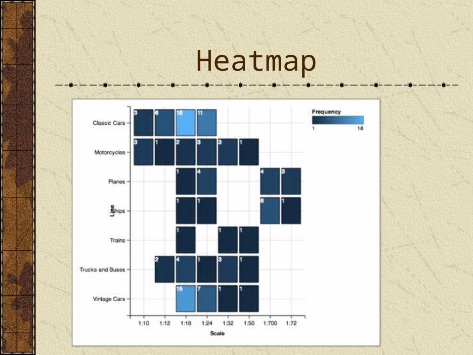
Heatmaplibrary(ggvis)library(RMySQL)options(sqldf.driver = "SQLite") # to avoid conflict with RMySQL# Load the driverconn <- dbConnect(RMySQL::MySQL(), "richardtwatson.com", dbname="ClassicModels", user="db1", password="student")d <- dbGetQuery(conn,'SELECT count(*) as Frequency, productLine as Line, productScale as Scale from Products group by productLine, productScale')d %>% ggvis( ~Scale, ~Line, fill= ~Frequency) %>% layer_rects(width = band(), height = band()) %>% layer_text(text:=~Frequency, stroke:='white', align:='left', baseline:='top') # add frequency to each cell

Heatmap

Interactive graphics

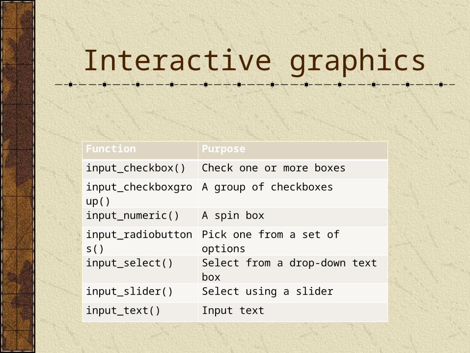
Function Purpose

input_checkbox() Check one or more boxes

input_checkboxgroup()

A group of checkboxes

input_numeric() A spin box

input_radiobuttons() Pick one from a set of options

input_select() Select from a drop-down text box

input_slider() Select using a slider

input_text() Input text

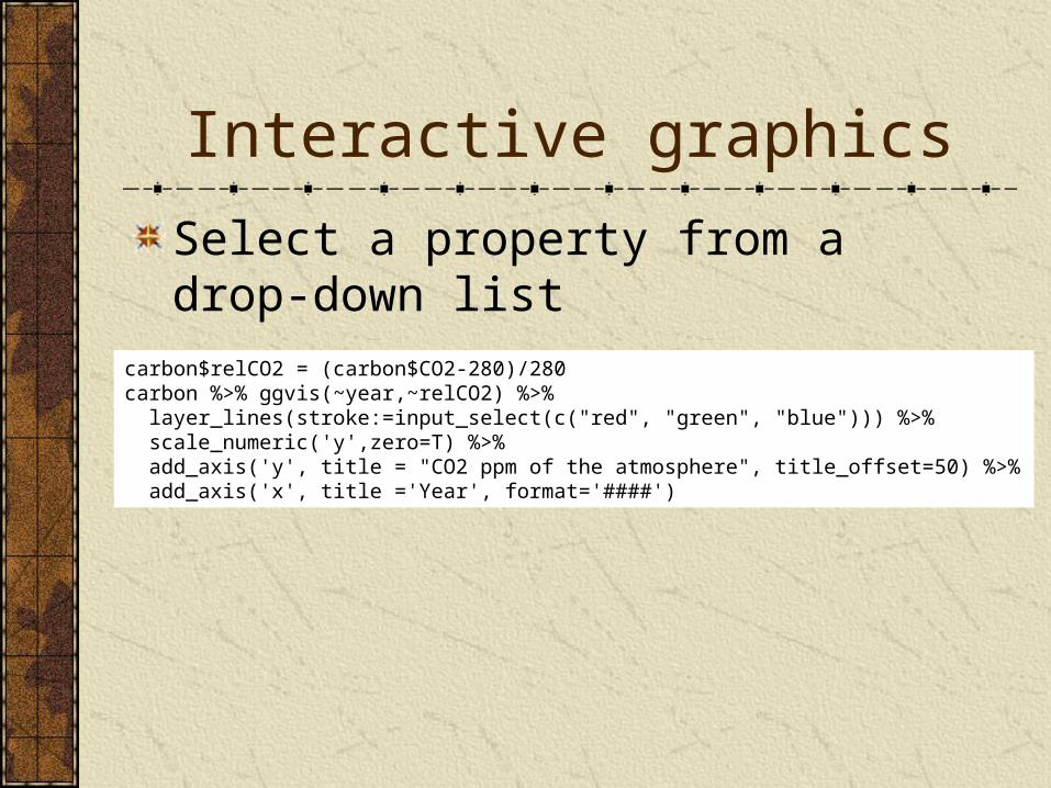
Interactive graphics

Select a property from a drop-down list

carbon$relCO2 = (carbon$CO2-280)/280carbon %>% ggvis(~year,~relCO2) %>% layer_lines(stroke:=input_select(c("red", "green", "blue"))) %>% scale_numeric('y',zero=T) %>% add_axis('y', title = "CO2 ppm of the atmosphere", title_offset=50) %>% add_axis('x', title ='Year', format='####')

Interactive graphics

Select a numeric value with a slider

carbon$relCO2 = (carbon$CO2-280)/280slider <- input_slider(1, 5, label = "Width")select_color <- input_select(label='Color',c("red", "green", "blue")) carbon %>% ggvis(~year,~relCO2) %>% layer_lines(stroke:=select_color, strokeWidth:=slider) %>% scale_numeric('y',zero=T) %>% add_axis('y', title = "CO2 ppm of the atmosphere", title_offset=50) %>% add_axis('x', title ='Year', format='####')

dplyr

Designed to work with ggvis and %>%

Function Purpose

filter() Select rows

select() Select columns

arrange() Sort rows

mutate() Add new columns

summarize()

Compute summary statistics

dplyrlibrary(sqldf)library(dplyr)options(sqldf.driver = "SQLite") # to avoid conflict with RMySQLurl <- 'http://people.terry.uga.edu/rwatson/data/centralparktemps.txt't <- read.table(url, header=T, sep=',')# filtersqldf("select * from t where year = 1999")filter(t,year==1999)# selectsqldf("select temperature from t")select(t,temperature)# a combination of filter and selectsqldf("select * from t where year > 1989 and year < 2000")select(t,year, month, temperature) %>% filter(year > 1989 & year < 2000)# arrangesqldf("select * from t order by year desc, month")arrange(t, desc(year),month)# mutate -- create a new columnt_SQL <- sqldf("select year, month, temperature, (temperature-32)*5/9 as CTemp from t")t_dplyr <- mutate(t,CTemp = (temperature-32)*5/9)# summarizesqldf("select avg(temperature) from t")summarize(t,mean(temperature))

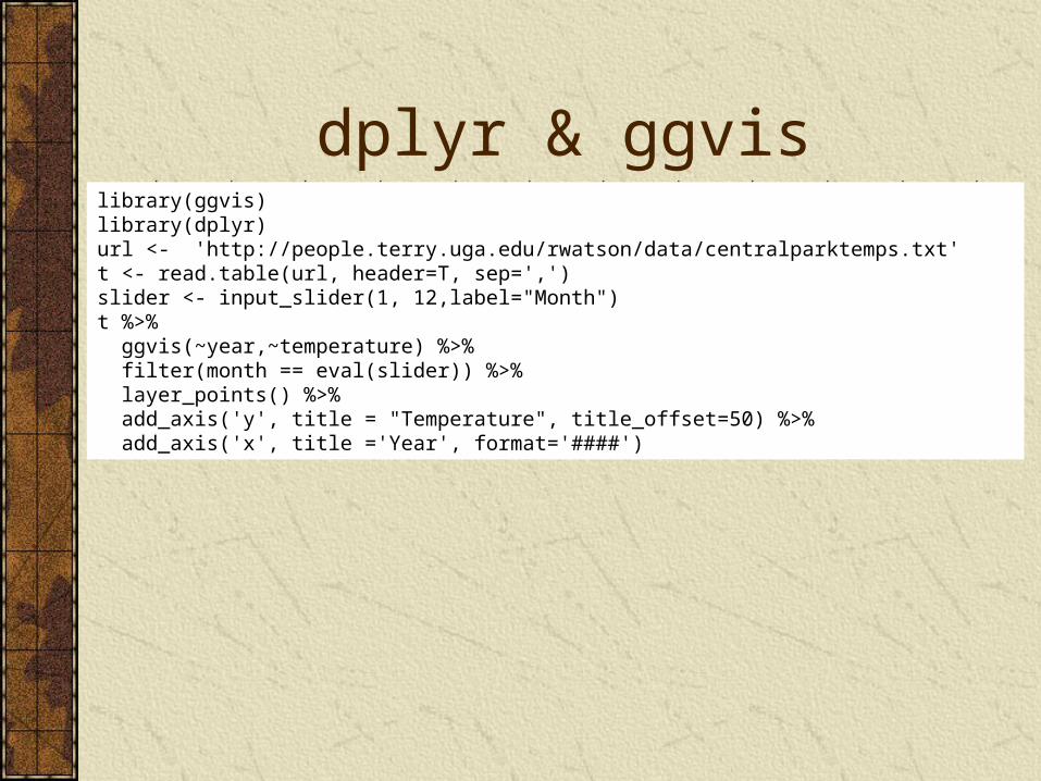
dplyr & ggvislibrary(ggvis)library(dplyr)url <- 'http://people.terry.uga.edu/rwatson/data/centralparktemps.txt't <- read.table(url, header=T, sep=',')slider <- input_slider(1, 12,label="Month")t %>% ggvis(~year,~temperature) %>% filter(month == eval(slider)) %>% layer_points() %>% add_axis('y', title = "Temperature", title_offset=50) %>% add_axis('x', title ='Year', format='####')

Geographic data

ggmap supports multiple mapping systems, including Google maps

library(ggplot)library(ggmap)library(mapproj)library(RMySQL)options(sqldf.driver = "SQLite") # to avoid conflict with RMySQl# connect to the databaseconn <- dbConnect(RMySQL::MySQL(), "richardtwatson.com", dbname="ClassicModels", user="db1", password="student")# Google maps requires lon and lat, in that order, to create markersd <- dbGetQuery(conn,"SELECT y(officeLocation) AS lon, x(officeLocation) AS lat FROM Offices;")# show offices in the United States# vary zoom to change the size of the mapmap <- get_googlemap('united states',marker=d,zoom=4)ggmap(map) + labs(x = 'Longitude', y = 'Latitude') + ggtitle('US offices')

Map

John Snow1854 Broad Street cholera map

Water pump

Cholera map(now Broadwick Street)

library(ggplot2)library(ggmap)library(mapproj)url <- 'http://people.terry.uga.edu/rwatson/data/pumps.csv'pumps <- read.table(url, header=T, sep=',')url <- 'http://people.terry.uga.edu/rwatson/data/deaths.csv'deaths <- read.table(url, header=T, sep=',')map <- get_googlemap('broadwick street, london, united kingdom',markers=pumps,zoom=15)ggmap(map) + labs(x = 'Longitude', y = 'Latitude') + ggtitle('Pumps and deaths') + geom_point(aes(x=longitude,y=latitude,size=count),color='blue',data=deaths) + xlim(-.14,-.13) + ylim(51.51,51.516)

Florence Nightingale

Florence Nightingale(code)

Key points

ggvis is based on a grammar of graphics

Very powerful and logicalSupports interactive graphics

You can visualize the results of SQL queries using RThe combination of MySQL and R provides a strong platform for data reporting