Data Structures, Optimal Choice of Parameters, and Complexity Results for Generalized Multilevel

Data Structures, Optimal Choice of Parameters, and Complexity Results for

Generalized Multilevel Fast Multipole Methods in � Dimensions

Nail A. Gumerov,� Ramani Duraiswami,� and Eugene A. Borovikov�

Perceptual Interfaces and Reality Laboratory,

Institute for Advanced Computer Studies,

University of Maryland, College Park, Maryland, 20742.

AbstractWe present an overview of the Fast Multipole Method, explain the use of optimal data structures and

present complexity results for the algorithm. We explain how octree structures and bit interleaving can

be simply used to create efficient versions of the multipole algorithm in � dimensions. We then present

simulations that demonstrate various aspects of the algorithm, including optimal selection of the cluster-

ing parameter, the in�uence of the error bound on the complexity, and others. The use of these optimal

parameters results in a many-fold speed-up of the FMM, and prove very useful in practice.

This report also serves to introduce the background necessary to learn and use the generalized FMM code

we have developed.

�URL: http://www.umiacs.umd.edu/~gumerov� Electronic address: [email protected]�URL: http://www.umiacs.umd.edu/~ramani� Electronic address: [email protected]�URL: http://www.umiacs.umd.edu/~yab� Electronic address: [email protected]

1

Contents

I. Introduction and scope of present work 4

A. The FMM Algorithm 5

II. Multilevel FMM 9

A. Statement of the problem and definitions 9

B. Setting up the hierarchical data structure 14

1. Generalized octrees (2� trees) 14

2. Data hierarchies 17

3. Hierarchical spatial domains 18

4. Size of the neighborhood 20

C. MLFMM Procedure 22

1. Upward Pass 22

2. Downward Pass 24

3. Final Summation 26

D. Reduced S�R-translation scheme 26

1. Reduced scheme for 1-neighborhoods 26

2. Reduced scheme for 2-neighborhoods 28

3. Reduced scheme for �-neighborhoods 30

III. Data structures and efficient implementation 32

A. Indexing 33

B. Spatial Ordering 36

1. Scaling 36

2. Ordering in 1-Dimension (binary ordering) 37

3. Ordering in �-dimensions 39

C. Structuring data sets 44

1. Ordering of �-dimensional data 45

2. Determination of the threshold level 46

3. Search procedures and operations on point sets 46

IV. Complexity of the MLFMM and optimization of the algorithm 47

2

The Fast Multipole Method 3

A. Complexity of the MLFMM procedure 47

1. Regular mesh 47

2. Non-uniform data and use of data hierarchies 50

B. Optimization of the MLFMM 51

V. Numerical Experiments 60

A. Regular Mesh of Data Points 60

B. Random Distributions 73

VI. Conclusions 77

Acknowledgments 80

References 80

VII. Appendix A 82

A. Translation Operators 82

1. R�R-operator 83

2. S�S-operator 83

3. S�R-operator 84

B. S-expansion Error 84

C. Translation Errors 85

1. R�R-translation error 85

2. S�S-translation error 86

3. S�R-translation error 87

VIII. Appendix B 88

A. S-expansion Error 88

B. S�R-translation Error 89

C. MLFMM Error in Asymptotic Model 89

c�Gumerov, Duraiswami, Borovikov, 2002-2003


I. INTRODUCTION AND SCOPE OF PRESENTWORK

Since the work of Greengard and Rokhlin (1987) [8], the Fast Multipole Method, has been es-

tablished as a very efficient algorithm that enables the solution of many practical problems that

were hitherto unsolvable. In the sense that it speeds up particular dense-matrix vector multipli-

cations, it is similar to the FFT,1 and in addition it is complementary to the FFT in that it often

works for those problems to which the FFT cannot be applied. The FMM is an “analysis-based”

transform that represents a fundamentally new way for computing particular dense-matrix vector

products, and has been included in a list of the top ten numerical algorithms invented in the 20th

century [9].

Originally this method was developed for the fast summation of the potential fields generated by

a large number of sources (charges), such as those arising in gravitational or electrostatic potential

problems, that are described by the Laplace equation in 2 or 3 dimensions. This lead to the name for

the algorithm. Later, this method was extended to other potential problems, such as those arising

in the solution of the Helmholtz [10, 11] and/or Maxwell equations [12]. The FMM has also

found application in many other problems, e.g. in statistics [13–15], chemistry [16], interpolation

of scattered data [17] as a method for fast summation of particular types of radial-basis functions

[18, 19].

Despite its great promise and reasonably wide research application, in the authors’ opinion, the

FMM is not as widely used an algorithm as it should be, and is considered by many to be hard to

implement. In part this may be due to the fact that this is a truly inter-disciplinary algorithm. It

requires an understanding of both the properties of particular special functions such as the transla-

tion properties multipole solutions of classical equations of physics, and at the same time requires

an appreciation of tree data-structures, and efficient algorithms for search. Further, most people

implementing the algorithm are interested in solving a particular problem, and not in generalizing

the algorithm, or explicitly setting forth the details of the algorithm in a manner that is easy for

readers to implement.

In contrast in this report we will discuss the FMM in a general setting, and treat it as a method

for the acceleration of particular matrix vector products, where we will not consider matrices that

1 Unlike the FFT, for most applications of the FMM there is no fast algorithm for inverting the transform, i.e., solvingfor the coefficients.



arise in particular applications. Further we present a prescription for implementing data-structures

that ensure efficient implementation of the FMM, and establish a clean description and notation

for the algorithm. Such a description is the proper setting to determine optimal versions of the

FMM for specific problems (variation of the algorithm with problem dimension, with clustered

data, and for particular types of functions �� These issues are both crucial to the implementation

of the algorithm, and its practical complexity.

Further, these issues are also a significant hurdle for those not familiar with data-structures,

such as engineers, applied mathematicians and physicists involved in scientific computation. Of

course, some of these details can also be gleaned from the standard texts on spatial data-structures

[1, 2], albeit not in the context of the FMM. A final issue is that our descriptions are not restricted

to 2 or 3 dimensional problems, as is usual, but are presented in the �-dimensional context. This

allows the same “shell” of the algorithm to be used for multiple problems, with only the translation

and the function routines having to be changed.

This report will only deal with what we refer to as the “regular multilevel FMM,” that employs

regular hierarchical data structures in the form of quad-trees in 2-D, octrees in 3-D, and their higher

dimensional generalizations. In a later report we hope to deal with a new adaptive FMM method

we have developed that achieves even better performance, by working with the point distributions

of both the source data and evaluation data, generalizing the multilevel adaptive FMM work that

has been presented in the literature (e.g., Cheng at al, 1999).

A. The FMM Algorithm

We first present a short informal description of the FMM algorithm for matrix-vector multi-

plication, before introducing the algorithm more formally. Consider the sum, or matrix vector

product

��

��

�� (1)

Direct evaluation of the product requires �� operations.

In the FMM, we assume that the functions � that constitute the matrix can be expanded as local



(regular) series or multipole (singular) series that are centered at locations �� and �� as follows:

��

��

��

��

��

where �� and �� are local (regular) and multipole (singular) basis functions, �� and �� are expan-

sion centers and �� are the expansion coefficients.

The Middleman method, which is applicable only to functions that can be represented by a

single uniform expansion everywhere (say an expansion in terms of the � basis above). In this

case we can perform the summation efficiently by first performing a � term expansion for each of

the � functions, �� at a point �� in the domain (e.g., near the center) requiring �� operations.

��

��

��

��

�� (2)

We consolidate the � series into one � term series, by rearranging the order of summation, and

summing all the coefficients over the index � requiring �� additions:

��

��

��

��

��

��

��

��

The single consolidated � terms series can be evaluated at all the evaluation points of the domain

in �� operations. The total number of operations required is then ��

for � � � The truncation number � depends on the desired accuracy alone, and is independent

of ��

We can recognize that the trick that allows the order of summation to be changed, will work

with any representation that has scalar product structure. We can represent the above summation

order trick as

��

��

�� (3)

where �� is an arbitrary point.

Unfortunately such single series are not usually available, and we may have many local or

far-field expansions. This leads to the idea of the FMM. In the FMM we construct the � and �

expansions, around centers of expansions, and add the notion of translating series. We assume we



have translation operators that relate the expansion coefficients in different bases, e.g.

��

��

��

where �� and �� denote translation operators that transform the coefficients be-

tween respective bases.

Given these series representations and translation operators, the FMM proceeds as follows.

First the space is partitioned into boxes at various levels, and outer � expansions computed about

box centers at the finest level, for points within the box. These expansions are consolidated, and

they are translated �� using translations in an upward pass up the hierarchy. The coefficients of

these box-centered expansions at each level are stored. In the downward pass, the consolidated �

expansions are expanded as local � expansions about boxes in the evaluation hierarchy, using the

�� translation, for boxes for which the expansion is valid (it is in the domain of validity of the

particular � expansion). At finer levels, the � expansions at the higher levels are �� translated

to the new box centers and to these are added the coefficients of the �� translations from boxes

at finer levels of the source hierarchy, which were excluded at the previous level(s). At the finest

level of the evaluation hierarchy we have � expansions about the box centers, and very few points

for which valid expansions could not be constructed. These are evaluated directly and added to the

� expansions evaluated at the evaluation points. Schematically the MLFMM, straightforward and

Middleman methods for matrix-vector multiplication are shown in Figure 1.

The FMM is thus a method of grouping and translation of functions generated by each source

to reduce the asymptotic complexity of finding the sum (3) approximately. The straightforward

computation of that sum requires �� operations, whereas the FMM seeks to approximately

compute these in �� or �� operations, by using the factorization and trans-

lation properties of ��. To achieve this, the original (classical) FMM utilizes a grouping based

on 2�-tree space subdivision. In the following we provide methods for doing this when both the

evaluation points and sources lie in the ��dimensional hypercube � � � � �� We will set

up the notation and framework to discuss optimizations of the algorithm possible, and characterize

the complexity of these versions of the algorithm.



N M

N M N M

MLFMM

Straightforward Middleman

N MN M

N MN M N MN M

MLFMM

Straightforward Middleman

FIG. 1: Schematic of different methods that can be used for multiplication of � � � dense matrix by a

vector of length � . In the straightforward method the number of operations is �� because of the

� sources is evaluated at the � evaluation points. The number of operations (connecting lines) can be

reduced to�� for the MLFMM and Middleman methods. The Middleman method can be used in a

limited number of cases when there exists a uniformly valid expansion for the entire computational domain.

The MLFMM is more general, since it also can be to the case of functions for which expansions only in

subdomains are applicable. The scheme for MLFMM shows only S�R translations on the coarsest level, S�R

translations from source hierarchy to the evaluation hierarchy at finer levels are not shown for simplicity of

illustration.



II. MULTILEVEL FMM

We present a formal description of the basic spatial grouping operations involved in the imple-

mentation of the fast multipole method and consider efficient methods for their implementation

using 2�-tree data-structures.

A. Statement of the problem and definitions

The FMM can be considered as a method for achieving fast multiplication of vectors with dense

matrices that have special structure, e.g., their elements can be written as �� where

�� and �� are points in �-dimensional Euclidean space. These points are usually called the “set of

sources”, �, and the set of “evaluation points” or “targets” � :

� � �� (4)

� � �� (5)

In general one seeks to evaluate the sum, or matrix-vector product

��

�� (6)

where �� are scalars (can be complex), and the contribution of a single source located at ��

is described by a function

�� (7)

Common examples of functions �� arising in FMM applications are �� (the fun-

damental solution of the 3D Laplace equation) or �� (a radial basis function in

�-dimensions).

For use with the FMM the functions �� must have the following properties:

� Local expansion (also called inner or regular expansion). The function �� can be evalu-

ated directly or via the series representation near an arbitrary spatial point �� as

�� (8)



Here the series is valid in the domain �� (see Fig. 2), where � � � �

is some real number. In general � depends on the function �� and its properties. � and� are

the basis functions and the series coefficients, represented as tensor objects in �-dimensional

space �� (for example, vectors of length �) and � denotes a contraction operation between

these objects, distributive with addition (for example, the scalar product of vectors of length

�):

�� (9)

Concerning the tensor function �� which can be interpreted as a set of basis func-

tions, we assume that it is regular at � � �� and that the local expansion is valid in-

side a �-dimensional sphere centered at � � �� with radius � �� The tensor object

��can be interpreted as a set of expansion coefficients for the basis.

� Far field expansion (also called outer, singular, or multipole expansion). Any function ��

has a complementary expansion valid outside a �-dimensional sphere centered at � � ��with radius � ��

�� (10)

where � � � is a real number similar to �� and the tensor function �� provides a

basis for the outer domain, and � is an operation similar to that in Eq. (8), that is distributive

with addition (see Eq. (9)). Even though for many physical fields, such as the Green’s

function for Laplace’s equation, the function �� is singular at � � �� this condition

is not necessary. In particular we can have � ��

The domains of validity of the expansions are shown in Figure 2.

� Translations.

The function �� may be expressed both as a far-field and a near-field expansion (series) as

in Equations (8) and (10) that are centered at a particular location ��The function can also be

expressed as in terms of a basis centered at another center of expansion ��. Both representations

evaluate to the same value in their domains of validity. The conversion of one representation, in one



xi

Ω

Ω

x*

R Sy

y

rc|xi - x*|

Rc|xi - x*|

xi

Ω

ΩΩ

x*

R Sy

y

rc|xi - x*|

Rc|xi - x*|

FIG. 2: Domains of validity of the regular (�, local) and singular (�, far field) expansions.

coordinate system with a particular center, to another representation in another coordinate system,

with another center is termed as a translation. The translation operator is a linear operator that

can be defined either in terms of the functions being translated or in terms of the coefficients of

their representations in a suitable local basis. The definition of the operator in terms of functions

is

�� (11)

where � is the translation vector, and �� is translation transform of �� For functions expandable over

the bases � and the action of the translation operators can also be represented by the action of

linear transforms on the space of coefficients. Depending on the expansion basis we consider the

following three types of translations, which are employed in the multilevel FMM:

1. Local-to-local (see Fig. 3). Consider the local expansion (8) near the point ��, which is

valid for any � �� If we choose a new center for the local

expansion, �� for � �� where �� is a sphere,

�� (12)

then the set of expansion coefficients transforms as

�� (13)



where �� is the local-to-local translation operator (or regular-to-regular, de-

noted by the symbol ��). Note that since � � � �� we have

� ��

Therefore, �� and the condition � ��

yields

��

The condition � �� is sufficient for validity of the local expansion (8) near point

��

xi

Ω1i

Ω2i

x*1

x*2

R (R|R)

y R

rc|xi - x*1|

xi

Ω1i

Ω2i

x*1

x*2

R (R|R)

y R

rc|xi - x*1|

FIG. 3: Local-to-local (or regular-to-regular) translation.

2. Far-to-local (see 4). Similarly, consider the far-field expansion (10) near the point ��, which

is valid for any � �� and select a center for a local

expansion at �� Then for � �� where �� is the sphere,

�� (14)

the set of expansion coefficients transforms as

�� (15)



where �� is the far-to-local translation operator (or singular-to-regular, de-

noted by the symbol ��). Note that the condition ��

provides that �� , and therefore the far field expansion is valid in �� The condition

�� ensures that the local expansion is valid in ��

xi

Ω1i

Ω1i

Ω2i

x*1

x*2

S

(S|R)

y

R

Rc|xi - x*1|

R2 = min{|x*2 - x*1|-Rc |xi - x*1|,rc|xi - x*2|}

R2

xi

Ω1i

Ω1iΩ1i

Ω2i

x*1

x*2

S

(S|R)

y

R

Rc|xi - x*1|

R2 = min{|x*2 - x*1|-Rc |xi - x*1|,rc|xi - x*2|}

R2

FIG. 4: Far-to-local (or singular-to-regular) translation.

3. Far-to-far (see Fig. 5). Finally, consider the far field expansion (10) near the point ��,

which is valid for any � �� and select a center �� for another far field expansion, where �� is a sphere that includes �� The far

field expansion near �� can be translated to the far field expansion near ��, if the evaluation

point � �� where �� is the external region of sphere �� such that :

�� (16)

The set of expansion coefficients then translates as

� �� (17)

where �� is the far-to-far field (or singular-to-singular, denoted by the symbol

�) translation operator. Note that

� ��



xi

Ω1i

Ω1i

Ω2i

x*1

x*2

S

(S|S)

y

S

Ω2i

Rc|xi - x*1|

xi

Ω1i

Ω1iΩ1i

Ω2i

x*1

x*2

S

(S|S)

y

S

Ω2iΩ2i

Rc|xi - x*1|

FIG. 5: Far-to-far (or singular-to-singular) translation.

Therefore, the definition of �� provides �� , and the condition for

the validity of the far field expansion near a new center is satisfied.

As mentioned above the translation operators are linear, which means that

�� (18)

where �� and�� are the expansion coefficients for expansions centered at �� with respect to the

basis �� and �� are the expansion coefficients for expansions centered at �� with respect to

the basis � and ��, �� are constants.

B. Setting up the hierarchical data structure

1. Generalized octrees (2� trees)

One of the most important properties of �-dimensional Euclidean space (��) is that it can be

subdivided into rectangular boxes (we are mostly concerned with cubes). In practice, the problems

we are concerned with are posed on finite domains, which can then be enclosed in a bounding box.

We assign this bounding box to level 0, in a hierarchical division scheme. The level 0 box can



be subdivided into �� smaller boxes of equal size by dividing each side in half. All boxes of this

size are assigned to level 1. Repeating this procedure, we produce a sequence of boxes at level 2,

level 3, and so on. While this process of sub-division could continue for ever, in practice we would

stop at some finite level ��, which is determined by some criterion (e.g., that there are at least

� particles in a box at the finest level). Figure 6, left, illustrates this for � � �. By the process

of division we obtain a ��-tree (see Figure 7), in which each node corresponds to a box. Any two

nodes at different levels are connected in the tree if the box corresponding to the first node at the

finer level is obtained by subdivision of the box corresponding to the second node at the coarser

level. At level � of a 2�-tree we have �� boxes, with each node having the index as �� with �

ranging from to �� Therefore any box in a 2�-tree can be characterized by the pair ��

Level 1

Level 0Level 2

Level 3

ParentSelf

ChildChild

Child Child

Neighbor(Sibling)

Neighbor Neighbor Neighbor

Neighbor

NeighborNeighbor(Sibling)

Neighbor(Sibling)

Level 1

Level 0Level 2

Level 3

Level 1

Level 0Level 2

Level 3

ParentSelf

ChildChild

Child Child

Neighbor(Sibling)

Neighbor Neighbor Neighbor

Neighbor

NeighborNeighbor(Sibling)

Neighbor(Sibling)

FIG. 6: The left graph shows levels in quad-tree space subdivision. The right graph shows children, parent,

siblings, and neighbors of the box marked as “self”.

A 2�-tree graph clearly displays “parent-child” relationships, where the “children” boxes at

level � � � are obtained by subdivision of a “parent” box at level �. For a 2�-tree with �� levels,

any box at level � � � has exactly one parent, and any box at level � � �� has exactly ��

children. So we can define operations � � �! �� which returns the index of the parent box,

and �"�� #�� that returns the indexes of the children boxes. The children of the same

parent are called “siblings”. Each box at a given level � � � has �� siblings.

In the FMM we are also interested in neighbor relationships between boxes. These are deter-

mined exclusively by the relative spatial locations of the boxes, and not by their locations in the



tree. We call two different boxes “neighbors” (or 1-neighbors) if their boundaries have at least

one common point. We also define 2-neighbors, 3-neighbors, and so on. Two different boxes are

2-neighbors if they are not 1-neighbors, but they have at least one common 1-neighbor. Two dif-

ferent boxes are 3-neighbors if they are not 1-neighbors, and not 2-neighbors, while at least one of

the neighbors of each box is a 2-neighbor of the other box, and so on up to the “�-neighborhood”,

� � �� . By induction the �-neighborhood is a union of two sets: the (� � �)-neighborhood

of the box and all its �-neighbors. We also use the terminology “power of a set” and “power of a

neighborhood” to denote the number of boxes in a particular set and number of boxes in a particular

neighborhood, respectively. For example, the power of the 0-neighborhood is 1.

The number of neighbors that a given box has in a finite 2�-tree space subdivision depends

on its location relative to the boundary of the domain (the boundaries of the box at level 0). For

example a box at level � � � in a quadtree situated at the corner of the largest box has only three

neighbors, while a box situated far from the boundaries (indicated as “self” in Figure 6, right) has

8 neighbors. The number of neighbors depends on the dimension �� In the general �-dimensional

case the minimum and maximum numbers of neighbors are

��

�� (19)

The minimum number of neighbors is achieved for a box in the corner, for which all neighbors

are children of the same parent (siblings). Since the number of siblings is �� this provides the

minimum number of neighbors . The maximum number of neighbors is for a box located far from

the boundary. Consider a box not on the boundary at a higher level. It has right and left neighbors

in each dimension, and can be considered the central box of a cube divided into ��

sub-boxes, which is the power of the 1-neighborhood. Excluding the box itself from this count we

obtain the number of its neighbors as in Eq. (19).

Equations (19) show that the number of neighbors for large � far exceeds the number of siblings.

The neighbor relationships are not easily determined by position on the 2�-tree graph (see Figure

7) and potentially any two boxes at the same level could be neighbors. On this graph the neighbors

can be close to each other (siblings), or very far apart, so that a connecting path between them may

have to go through a higher node (even through the node at level 0). For further consideration we

can introduce operation � �$"�%��#�� which returns indexes of all �-neighbors of the box

�� .



2-tree (binary) 22-tree (quad) 2d-tree

0

1

2

3

Level

Children

Parent

Neighbor(Sibling) Maybe

Neighbor

Self

Numberof Boxes

1

2d

22d

23d

2-tree (binary) 22-tree (quad) 2d-tree

0

1

2

3

Level

Children

Parent

Neighbor(Sibling) Maybe

Neighbor

Self

Numberof Boxes

1

2d

22d

23d

FIG. 7: 2�-trees and terminology.

The example above shows that the power of �-neighborhood depends on the level and on the

location of the box. The maximum value of the power of �-neighborhood is

&�%' ��-� �$"�%�"%%�� (20)

This shows that at fixed � the power depends polynomially on �� while at fixed � it depends

exponentially on the dimension �.

2. Data hierarchies

The 2�-trees provide a space subdivision without any consideration for the distribution of the

source and evaluation data points (4) and (5). These data can be structured with 2�-trees and orga-

nized in the (-data hierarchy (or source hierarchy) and the ) -data hierarchy (or evaluation/target

hierarchy) according to the coordinates of the source and evaluation points. We prescribe to each

source or evaluation point the index of the box �� to which it belongs, so that ( and ) are sets

of indices ��

For each data hierarchy we define the operations � � �!�� "�� and

� �$"�%�� The operation � � �!�� is the same for both hierarchies, since the par-

ent of each box already contain points of the hierarchy. The other two operations return the sets of



children and �-neighbor boxes at levels � � � and �, respectively, that contain the points from the

particular hierarchies. To discriminate between the two sets, we denote them as �"�� (��

and � �$"�%�� (�� for the (-hierarchy and �"�� ) �� and � �$"�%�� ) ��

for the ) -hierarchy.

3. Hierarchical spatial domains

We define notation here that will permit a succinct description of the FMM algorithm, and

further allow for its optimization. By optimization we mean the selection of parameters, e.g., one

of the parameters to be chosen is the number of points, �� that are contained at the finest level

�� in a non-empty box.

We define the following four spatial domains that are used in the FMM. These can be defined

for each box with index � � � �� at level � � � �� and have fractal structure2:

� *� �� denotes spatial points inside the box ��

� *�� denotes spatial points in the �-neighborhood (� � �� ) of box ��

� *� �� *� � � � �*

�� denotes spatial points outside the �-neighborhood (� �

�� ) of box ��

� *�� *

�� !�� *�

� �� denotes spatial points in the �-

neighborhood of the parent box �� !�� which do not belong to the �-

neighborhood of the parent box itself.

We, thus associate with each other the sets of boxes at level � that constitute each of the domains

*� �� , + � �� which we denote as ,�� Boxes ,�� ( and ,�� ) belong

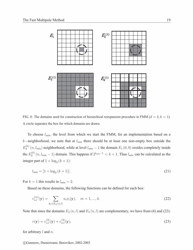
to the ( and ) hierarchies, respectively. Figure 8 illustrates these domains in the case � � � and

� � �� Each FMM algorithm could in principle be based on one of these �-neighborhoods, though

most FMM algorithms published thus far have used 1-neighborhoods.

2 By fractal we mean that these structures have the same shape at different levels of the hierarchy.



Ε1

Ε3(1) Ε4

(1)

Ε2(1)Ε1

Ε3(1) Ε4

(1)

Ε2(1)

FIG. 8: The domains used for construction of hierarchical reexpansion procedure in FMM (� � �� ).

A circle separates the box for which domains are drawn.

To choose �� the level from which we start the FMM, for an implementation based on a

��neighborhood, we note that at �� there should be at least one non-empty box outside the

*�� neighborhood, while at level �� the domain *� � � � resides completely inside

the *�� domain� This happens if �� Thus �� can be calculated as the

integer part of � � �� :

�� (21)

For � � � this results in ��

Based on these domains, the following functions can be defined for each box:

��

��

�� - � �� (22)

Note that since the domains *� �� and * �� are complementary, we have from (6) and (22):

��

�� (23)

for arbitrary � and ��



4. Size of the neighborhood

The size of the neighborhood, �, must be determined before running the MLFMM procedure.

The choice is based on the space dimensionality and parameters � and �� which specify the

regions of expansion validity.

1. The �-expansion (10) near the center of the �th box at level � for �� *� �� is valid

for any � in the domain *� �� In �-dimensional space the maximum distance from the

center of the unit box to its boundary is ��.� and the minimum distance from the center to

the boundary of its �-neighborhood domain (*� �� ) is �� .�� Therefore � should

be selected so that

� � �

�

��

�� (24)

For example, for � � �� and � � �� this condition yields � � �� so � � � can be

used, while for � � �� we have � � �� and the minimum integer � that satisfies

Eq. (24) is �.

2. The �-expansion (8) near the center of the �th box at level � for �� *� �� is valid for

any � from the domain *� �� A similar calculation as that lead to Eq. (24) leads to the

following selection criteria for �:

� � �

�

��

��

� (25)

Therefore these two requirements will be satisfied simultaneously if

� � �

�

��

��

��

��

�� (26)

3. The ��-translation (17) of the �-expansion from the center of the �th box at level � for

�� *� �� to the center of its parent box preserves the validity of the �-expansion for

any � from the domain *� �� !�� Eq. (16) shows that this condition is

satisfied if Eq. (24) holds.

4. The ��-translation (13) of the �-expansion from the center of the �th box at level � for

�� *� �� to the centers of its children preserves the validity of the �-expansion for

any � from the domain *� ��"�� #�� Eq. (12) shows that this condition is

satisfied if Eq. (25) holds.



5. The ��-translation (15) of the �-expansion from the center of the -th box at level � which

belongs to *�� for �� *� �-� �� to the center of the box *� �� provides a valid

�-expansion for any � from the domain *�� If the size of the box at level � is 1, then

the minimum distance between the centers of boxes �-� �� (say ��) and �� (say ��), is

� � �� The maximum �� is ��.�� the minimum �� is �� .�� and the

maximum �� is ��.�� Thus, condition (14) will be satisfied if

��

�� (27)

This also can be rewritten as

� � �

��

��

��

�

��

�� (28)

Combining Eq. (28) and Eq. (26) we obtain the following general condition for the selection

of the neighborhood size

� � �

��

��

��

��

��

��

��

�� (29)

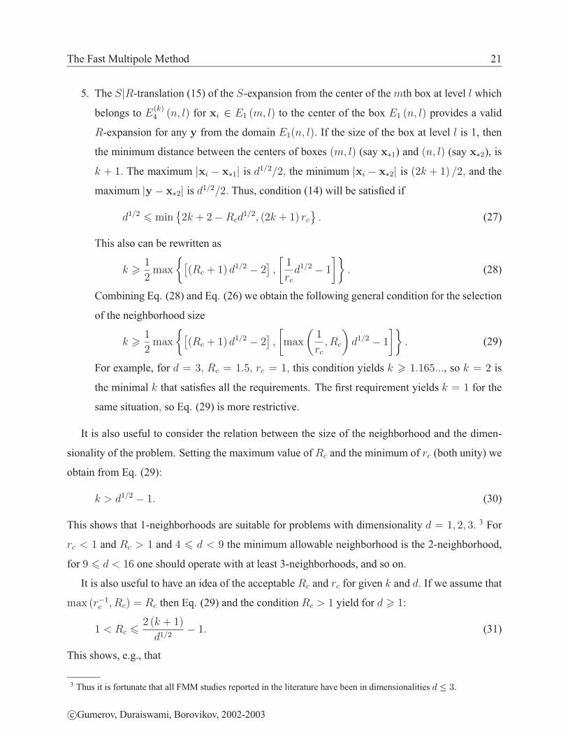
For example, for � � �� this condition yields � � ��, so � � � is

the minimal � that satisfies all the requirements. The first requirement yields � � � for the

same situation� so Eq. (29) is more restrictive.

It is also useful to consider the relation between the size of the neighborhood and the dimen-

sionality of the problem. Setting the maximum value of � and the minimum of � (both unity) we

obtain from Eq. (29):

� � �� (30)

This shows that 1-neighborhoods are suitable for problems with dimensionality � � �� 3 For

� � � and � � � and � � � � � the minimum allowable neighborhood is the 2-neighborhood,

for � � � � �� one should operate with at least 3-neighborhoods, and so on.

It is also useful to have an idea of the acceptable � and � for given � and �� If we assume that

�� then Eq. (29) and the condition � � � yield for � � �:

� � � ��

�� (31)

This shows, e.g., that

3 Thus it is fortunate that all FMM studies reported in the literature have been in dimensionalities � � �



Neighborhood type (�� Dimensionality (�� Convergence radius, �1 1 � �

1 2 � � ��

1 3 � �.��

If the expansion (10) holds for larger � than is permitted by the minimum � for a given dimen-

sionality, then the size of the neighborhood should be increased. E.g., for � � � one can increase

� to � to extend � to � � �.�� . Note that this type of neighborhood was also

considered by Greengard in his dissertation [6], where the MLFMM was developed for 3D Laplace

equation, but has not been used by others since.

C. MLFMM Procedure

Assuming that condition (29) holds, so that all the translations required for the FMM can be

performed. The FMM procedure consists of an Upward Pass, which is performed for each box at

level �� up to the level �� of the (-hierarchy and uses the �-expansions for these boxes, in the

two step Downward Pass, which is performed for each box from level �� down to level �� of the

) -hierarchy and uses �-expansions for boxes of this hierarchy, and the Final Summation. Transla-

tions within the (-hierarchy are ��-reexpansions, within the ) -hierarchy are ��-reexpansions,

and translations from the boxes of the (-hierarchy to the boxes of the ) -hierarchy are the ��-

reexpansions.

1. Upward Pass

Step 1. For each box �� in the (-hierarchy, generate the coefficients of the �-expansion ,

�

��

�� for the function �

��

�� centered at the box-center, �� Multiply these

with the associated scalar in the vector being multiplied, and consolidate the coefficients of

all source points in the box to determine the expansion coefficients �� corresponding

to that box,

��

��

��

�� (� (32)�

��

��



Note that since the �-expansion is valid outside a region containing the center, because of

(24) the expansion (32) for the �th box is valid in the domain *� �� (see Fig. 8).

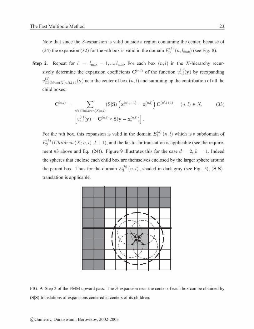
Step 2. Repeat for � � �� For each box �� in the (-hierarchy recur-

sively determine the expansion coefficients �� of the function �� by reexpanding

�� near the center of box �� and summing up the contribution of all the

child boxes:

��

��

��

��

��

�� (� (33)��

��

For the �th box, this expansion is valid in the domain *� �� which is a subdomain of

*� ��"�� (�� , and the far-to-far translation is applicable (see the require-

ment #3 above and Eq. (24)). Figure 9 illustrates this for the case � � �, � � �� Indeed

the spheres that enclose each child box are themselves enclosed by the larger sphere around

the parent box. Thus for the domain *� �� shaded in dark gray (see Fig. 5), ��-

translation is applicable.

FIG. 9: Step 2 of the FMM upward pass. The �-expansion near the center of each box can be obtained by

(S�S)-translations of expansions centered at centers of its children.



2. Downward Pass

The downward pass applies steps 1 and 2 below for each of the levels � � �� .

Step 1. In this step we form the coefficients, �� of the regular expansion for the function

�� about the center of box �� )� To build the local expansion near the center of

each box at level ��the coefficients�� ,�� ( should be ��- translated to

the center of the box. Thus we have

��

��

��

��

��

�� )� (34)

��

��

FIG. 10: Step 1 of the downward pass of the FMM. The coefficients of singular expansion corresponding

to dark gray boxes are (S�R)-translated to the center of the light gray box. Figures illustrate this step for

quadtree at levels 2 and 3.

Condition (27) ensures that the far-to-local translation (15) is applicable. Figure 10 illustrates this

step for � � � and � � ��



Step 2. Assuming that for � � ��

�� )��

��

�� (35)

we form the coefficients of the regular expansion �� for the function � �� about the

box center �� )� by adding �� to the coefficients obtained by ��- translation of

� �� from the parent box to the center of the child box �� :

��

��

�� !�� )��

� ��

�� (36)

For the �th box, this expansion is valid in the domain *� �� which is a subdomain of

FIG. 11: Step 2 of the downward pass of the FMM. On the left figire the coefficients of the parent box (light

gray) are locally translated to the center of the black box. On the right figure contribution of the light grey

boxes is added to the sum of the dark boxes to repeat the structure at the finer hierarchical level.

*� �� !�� , and the local-to-local translation is allowed (see the requirement

#4 above and Eq. (25)). Figure 11 illustrates this for � � �, � � �� Indeed the smaller

sphere is located completely inside the larger sphere), and junction of domains *� ��

and *�� produces *

� ��

*� �� *

� �� *

�� (37)



3. Final Summation

As soon as coefficients �� are determined, the total sum �� can be computed for any

point �� *� � � � using Eq. (23), where �� can be computed in a straightforward way, using

Eq. (22). Thus

��

��

�� *� �� (38)

D. Reduced S�R-translation scheme

Step 1 in the downward pass is the most expensive step in the algorithm since it requires a

large number of translations (from each box �� ,�� (). The maximum number of such

translations per box can be evaluated using Eq. (20) as

�� %' �� $"�%�"%%��%' �� $"�%�"%%�� (39)

��

��

where the first term in the difference represents the number of boxes at level � that belongs to the �-

neighborhood of the parent box and the second term is the number of boxes in the �-neighborhood

of the box itself.

We can substantially reduce the number of translations if we note that some translations are

performed from all the children boxes of a parent. For such boxes we can use the already known �-

expansion coefficients from the coarser level. However, such an operation reduction trick requires

an additional analysis to ensure that the expansion domains are valid.

1. Reduced scheme for 1-neighborhoods

Let us subdivide the set ,�� into two sets

,�� ,

�� ,

�� (40)

� � �!�,��

� � � �!

�� $"�%��

� ��

� � �!�,��

� � � �!

�� $"�%��

� ��



where ,�� is the set of boxes at level � whose parent boxes include boxes from the set�

� �$"�%�� and ,

�� is the set of boxes whose parents do not include the neigh-

bor boxes of �� (see Figure 12). Thus all boxes in the set ,�� can be grouped according

to their parents. The set � � �!�,��

�is a set of boxes of the coarser level, � � �, that are

located in the domain *�� but is separated from the box �� . Therefore, instead of Eq.

(34) we can write

��

��

��

��

��

�� (41)

��

��

��

��

��

��

�� )�

Note that for level � � � the latter sum in Eq. (41) should be set to zero, since the set

� � �!�,��

�is empty.

FIG. 12: Reduced scheme with 1-neighborhoods for the step 1 of the downward pass of the FMM. The

coefficients of the singular expansion corresponding to dark gray boxes are (S�R)-translated to the center of

the light gray box. For optimization the parent level coefficients can be used for boxes shown in deep dark

gray. This step is illustrated for a quadtree at levels 2 and 3.

Consider now the requirement for the validity of the ��-translation, Eq. (15), for such a

reduced scheme. If the size of the box at level � is 1, then the minimum distance between the

centers of boxes �-� � � �� which is the 1-neighbor of � � �! �� (say ��) and �� (say



��), is��

��

��

�� The maximum distance �� is �� the minimum

distance �� is �.� and the maximum distance �� is ��.�� The condition (14) will

thus be satisfied if

�� (42)

Even for � � � this requirement can be satisfied only if �� i.e. for � � � and

� � �� Hence the reduced scheme for 1-neighborhood is applicable only for these low dimensions.

For � � � it permits us to make two ��-translations instead of three for the regular translation

scheme with � � � � �� For � � � it permits us to make twelve ��-translations instead of

the 27 needed for the regular translation scheme with � � � ��

�.� �� Note

that the reduction of the range of possible convergence radii � (the maximum � in the reduced

scheme is � instead of � for � � � and �� instead of �� for � � �) is a cost that one has to

pay for the use of the reduced scheme.

2. Reduced scheme for 2-neighborhoods

Figure 13 illustrates the idea of the reduced translation scheme for 2-neighborhoods. Instead of

translating expansions from each gray box to the black box in the left figure, one can reduce the

number of translations by translating expansions from the centers of the parent boxes (shown in

darker gray) and smaller number of boxes at the same level (shown in lighter gray).

Again the total sum can be subdivided into two parts corresponding to the boxes at the same

level and the boxes at the parent level. The major issue here is determining the domains of validity

of the ��-translation (15). Extending the geometrical consideration to this case, we find that for

unit size boxes at level �, the minimum distance between the centers of boxes �� which is

the 2-neighbor of � � �! �� say �� and �� say ��, is��

��

��

�� The

maximum distance �� is �� the minimum distance �� is �.� and the maximum

distance �� is ��.�� The condition (14) will be satisfied if

�� (43)

The maximum possible space dimension can be found by letting � � �� which yields ��

�� and that the reduced translation scheme is valid for � � �� The maximum number of



FIG. 13: Regular (left) and reduced (right) schemes with 2-neighborhoods for step 1 of the downward pass

of the FMM. The coefficients of the singular expansion corresponding to the gray boxes are (S�R)-translated

to the center of the black box. For optimization the parent level coefficients can be used for boxes shown in

deep dark gray.

translations using the reduced scheme is ��

�� which is the same

as the number of translations with the regular scheme with 1-neighborhoods, Eq. (39), and less

than the regular scheme with �-neighborhoods by ��.�� times. This can be a substantial saving

for larger �� e.g. for � � � since this reduces the number of translations from 875 to 189, or more

than 4.6 times.

As in the case with 1-neighborhoods, the reduction in the number of translations is accompanied

by a reduction in the allowed dimensionality (the maximum � is 5 for the reduced scheme and 8

for the regular scheme), and the maximum radius of expansion validity, � (e.g. at � � � we have

� � �� for the regular scheme, see Eq. (31), and � ��

�.� �� for the

reduced scheme). However, we note that this range is larger than the range of allowable � for the

regular scheme using 1-neighborhoods, for which we have � � �� Taking into account that

the number of translations is the same for the reduced scheme with 2-neighborhoods and regular

scheme with 1-neighborhoods, we find that better convergence properties for the same amount of

operations can be achieved if the reduced scheme is used.



3. Reduced scheme for -neighborhoods

When we use FMM algorithms based on larger neighborhoods (�� the difference between the

�-neighborhood of the parent box (level � � �) and the box itself (level �) can be large enough, so

that we can group boxes not only of the parent level, but also boxes belonging to levels ��

and so on. Figure 14 illustrates three possible schemes of translations with 3-neighborhoods, the

regular (left), reduced with maximum size boxes at the parent level (center) and the maximum size

boxes at the parent of parent (or grandparent) level.

FIG. 14: Regular (left) and reduced to parent level (center) and to grandparent level (right) schemes with

3-neighborhoods for the step 1 of the downward pass of the FMM.

To check the validity of such schemes, first we note that the minimum distance from the unit

size box �� to the boundary of its *�� domain is �� while the distance to the boundary of

its *�� domain is �� The difference is �� and so the box of level �� can fit in this space

if � � �� The size of the box at this level is �� and we can consider

limitations for the space dimensionality and the convergence radius for the ��translation to be

performed from the box of size ��, � - � � � �� located right near the boundary of *��

Denoting the center of this box as �� and the center of box �� as �� we find that the

minimum distance between the centers is��

��

��

�

�� . The

maximum distance �� is �� the minimum distance �� is �� .� and the

maximum distance �� is ��.�� Condition (14) will be satisfied if

��

��

�� (44)



First, we can consider the dimensionality limits. Assuming � � �� we obtain

� ��

�� - � � �� (45)

The allowable dimension as a function of -, the size of the box allowed, � �-� � at fixed � decays

monotonically. We also recall that the maximum - that can be achieved is - � �� For a

reduced scheme using this value we obtain

� ��

�� (46)

which shows that in this case one should not expect that the reduced scheme will work for dimen-

sions larger then � � �� Therefore, for problems in larger dimensions one should select - � ��

Furthermore, we can obtain the following relation for the convergence radius as a function of

�� and - �

� � ��

� ��

�

��

�� - � � ��

(47)

This relation shows that the range of allowable � decreases when - and � increase, and increases

when � increases. In terms of reduction of the number of operations for given � and �� and -

should be selected to achieve the minimum possible � and maximum possible -�

We also note that for larger � there exist different possibilities for reduction of the number of

operations. Such schemes can be composed from boxes of levels �� and so on. The

general trend is that larger � and � can be treated when the scheme is designed so that smaller

boxes are located closer to the �-neighborhood of the box �� and larger boxes are located closer

to the boundary of the domain *��

The problem of efficient computational treatment of cases with larger dimensionality is still an

open one, since an increase in � leads to an increase of �� and the power of the �-neighborhood

(20) increases exponentially with �� Such cases can be treated however, if the number of sources in

such neighborhoods is much smaller than their maximum power, which is typical for problems

in higher dimensions. What is also typical for high � problems is that points usually cluster in

subspaces of lower dimensionality. In this case special grouping techniques that may include local

rotations can be considered as candidates for reduction of the number of operations.



III. DATA STRUCTURES AND EFFICIENT IMPLEMENTATION

Our goal is to achieve the matrix-vector multiplication, or sum, in Eq. (6) in �� or

�� operations. Accordingly all methods used to perform indexing and searching for

parent, children, and neighbors in the data hierarchies should be consistent with this. It is obvi-

ous that methods based on naive traversal algorithms have asymptotic complexity �� and are

not allowed since this would defeat the purpose of the FMM. There is also the issue of memory

complexity. If the size of the problem is small enough, then the neighbor search procedures on

trees can be �� and the complexity of the MLFMM procedure can be �� More restrictive

memory requirements bring the complexity of such operations to �� and the complexity of

the MLFMM procedure to �� Reduction of this complexity to �� can be achieved

in some cases using hashing (this technique however depends on the properties of the source and

evaluation data sets and may not always result in savings) [20].

From the preceding discussion, 2�-tree data structures are rather natural for use with MLFMM.

Since, the regions of expansion validity are specified in terms of Euclidean distance, subdivision

of space into �-dimensional cubes is convenient for range evaluation between points. We note that

in the spatial data-structure literature, the data-structures used most often for higher dimensional

spaces are �-� trees (e.g., see [1, 2]). Such structures could also be employed in the MLFMM,

especially for cases when expansions are tensor products of expansions with respect to each coor-

dinate, however no such attempts have been reported to our knowledge. We also can remark that

2�-tree data structures can be easily generated from �-� data structures, so methods based on �-�

trees can be used for the MLFMM. The relative merits of these and other spatial data-structures

for the FMM remain a subject for investigation.

The main technique for working with 2�-trees (and �-� trees) is the bit-interleaving technique

(perhaps, first mentioned by Peano in 1890 [3], see more details and the bibliography in [1, 2])

which we apply in �-dimensions. This technique enables ��, or constant, algorithms for parent

and sibling search and �� algorithms for neighbor and children search. Using the bit inter-

leaving technique the time complexity for the MLFMM is provide �� in case we wish to

minimize the amount of memory used. If we are able to store the occupancy maps for the given

data sets we can obtain �� complexity.

While these algorithms are well known in the spatial data-structures community they have not



been described in the context of the FMM before, and it is a lack of such a clear exposition that

has held back their wider use.

A. Indexing

To index the boxes in a more efficient way we can, for example, do the following. Each box in

the tree can be identified by assigning it a unique index among the �� children of its parent box, and

by knowing the index of its parent in the set of its grandparent’s children, and so on. For reasons

that will be clear in the next section we index the �� children of a particular parent box using the

numbers � �� . Then the index of a box can be written as the string

�!��$ �� (48)

where � is the level at which the indexed box is located and �� is the index of a box at level

containing that box. We drop �� from the indexing, since it is the only box at level � and has no

parents. We can assign the index 0 to this box.. For example, in two dimensions for the quad-tree

we have the numbering shown in Figure 15. The smaller black box will have indexing string (3,1,2)

and the larger black box will have indexing string (2,3). From the construction it is clear that each

box can be described by such a string, and each string uniquely determines the box.

0 01 2

1 31

3

3

3

31

1

1

0

20 0

02 2

2

1

11

1

1

111

11

11

1 1 1

0

0

0

00 0

0

0

0

0 00

0

0

0

2

0

2 2 2 2

222

2 2

222

2

2

2

3 3 3 3

3

3

3 33

3 3 3

33330 01 2

1 31

3

3

3

31

1

1

0

20 0

02 2

2

1

11

1

1

111

11

11

1 1 1

0

0

0

00 0

0

0

0

0 00

0

0

0

2

0

2 2 2 2

222

2 2

222

2

2

2

3 3 3 3

3

3

3 33

3 3 3

3333

FIG. 15: Hierarchical numbering in quad-tree.



The indexing string can be converted to a single number as follows:

� ��

� ��

� �� (49)

Note that this index depends on the level � at which the box is considered and unless this informa-

tion is included, different boxes could be described by the same index. For example, boxes with

strings (0,2,3) and (2,3) map to the same index, � � ��, but they are different. The box (0,2,3) is

the small grey box and (2,3) is the larger black box in Figure 15. The unique index of any box can

be represented by the pair:

/�� ,�� & � �� (50)

We could instead say “box 11 at level 2” (this is the larger black box in Figure 15) or “box 11 at

level 3” (this is the smaller gray box in Figure 15). We also have the box with index 0 at each level,

which is located in the left bottom corner. “Box 0 at level 0” refers to the largest box in the ��-tree.

The string could be mapped in a different way, so that all boxes map to a unique index, instead

of a pair. However, storing the level number, does not increase the memory or time complexity,

since anyway the MLFMM loops go through the level hierarchy, and one always has level value.

If the indexing at each level is performed in a consistent way (for example in Figure 15 we

always assign 0 to the child at the bottom left corner of the parent, 1 to the child in the left upper

corner, 2 to the child in the right bottom corner, and 3 to the child in the right upper corner� for

quad-trees this can be also called ‘0-order’ following [4]) then we call such a indexing scheme

“hierarchical.” A consistent hierarchical scheme has the following desirable properties.

1. Determining the Parent: Consider a box at level � of the ��-tree, whose index is given by Eq.

(49). The parent of this box is

� � �!��

� ��

� �� (51)

To obtain this index there is no need to know whether �� and so on are zeros or not.

We also do not need to know �� since this index is produced from string simply by dropping

the last element:

� � �! �� (52)

This means that function � � �! in such a numbering system is simple and level indepen-

dent. For example at � � � for box index �� the parent always will be � � �!��



� independent of the level being considered. Obtaining the parent’s index in the universal

numbering system in Equation (50) is also simple, since the level of the parent is � � ��

Therefore,

� � �! �� !�� (53)

2. Determining the Children: For the function �"�� #�� as well we do not need to know

the level. Indeed, to get the indices of all �� children of a box represented by the string (48),

we need simply add one more element to the string, which runs from to �� to list all

the children:

�"�� #�� (54)

or

�"�� #��

��

� ��

��

��

(55)

For the universal numbering system (50), the operation of finding the children is simply the

calculation of the children numbers and assigning their level to � � � �

�"�� #�� "�� #�� (56)

Note that

� � �!�� .��

�� (57)

�"�� #��

� � � �� (58)

where �� means integer part.

The use of ��-trees makes obtaining parent and children indices very convenient. Indeed the

above operations are nothing but shift operations in the bit representation of �� Performing a right

bit-shift operation on � by �-bits one can obtain the index of the parent. One can list all indices

of the children boxes of � by a left bit-shift operation on � by �-bits and adding all possible

combinations of �-bits.



B. Spatial Ordering

The above method of indexing provides a simple and natural way for representing a ��-tree

graph structure and easy �� algorithms to determine parent-children (and therefore sibling) re-

lationships. However, we still do not have a way for determining neighbors. Further the MLFMM

algorithm requires finding of the box center for a given index �� and the box index to which

a given spatial point � belongs. To do this a spatial ordering in �-dimensional space should be

introduced. We provide below such an ordering and �� algorithms for these operations.

1. Scaling

As assumed above, the part of the �-dimensional space we are interested in can be enclosed

within a bounding box with dimensions �� . In problems in physical space of

dimensions (� � �� ) we usually have isotropy of directions and can enclose that box in a cube

of size � � �� where

� � ��

�� (59)

with one corner assigned the minimum values of Cartesian coordinates:

�� &�� &�� (60)

This cube then can be mapped to the unit cube � � �� by a shift of the origin and scaling:

� ��

�� (61)

where the � are the true Cartesian coordinates of any point in the cube, and � are normalized

coordinates of the point. If a ��-tree data structure is applied to a case where each dimension has

its own scale �� (such problems are typical in parametric spaces) the mapping of the original box

�&�� &�� &�� &�� &�� &�� (62)

to the unit cube � � �� can be also easily performed by scaling along each dimension

as:

&� �&� � &��

�� &�� &��



In the sequel we will work only with the unit cube, assuming that, if necessary, such a scaling

has already been performed, and, that the point � in the original �-dimensional space can be found

given � � � � �� .

2. Ordering in 1-Dimension (binary ordering)

Let us consider first the case � � �� where our ��-tree becomes a binary tree (see Figure 6). In

the one-dimensional case all the points & � � � �� are naturally ordered and can be represented in

the decimal system as

& � � � � � �� (63)

Note that the point & � � can also be written as

& � � � � �� (64)

which we consider to be two equivalent representations. The latter representation re�ects the fact

that & � � is a limiting point of sequence 0,0.9,0.99, .

We also can represent any point & � � � �� in the binary system as

& � � �� (65)

and we can write the point & � � in the binary system as

& � � � � �� (66)

Even though the introduced indexing system for the boxes in the case � � �� results in a rather

trivial result, since all the boxes are already ordered by their indices at a given level � from to ��,

and there is a straightforward correspondence between box indices and coordinates of points, we

still consider the derivation of the neighbor, parent and children and other relationships in detail,

so as to conveniently extend them to the general �-dimensional case.

a. Finding the index of the box containing a given point. Consider the relation between the

coordinate of a point and the index of the box where the point is located. We note that the size of a

box at each level is � placed at the position equal to the level number after the decimal in its binary

record as shown in the table below.



Level Box Size (dec) Box Size (bin)

0 1 1

1 0.5 0.1

2 0.25 0.01

3 0.125 0.001

... ... ...

If we consider level 1 where there are two boxes:

� � �� 1%& �� 1%& �� (67)

where 1%&� � and 1%&�� denote sets of spatial points that belong to boxes with indices � � and

�� respectively (at this point we will use binary strings for indexing) . At level 2 we will have

� � �� 1%& �� 1%& �� (68)

� �� 1%& �� 1%& ��

��

This process can be continued. At the �th level we obtain

� �� 1%& �� (69)

Therefore to find the index of the box at level � to which the given point belongs we need simply

shift the binary number representing this point by � positions and take the integer part of this

number:

� �� (70)

This procedure also can be written as

�� &

�� (71)

b. Finding the center of a given box. The relation between the coordinate of the point and

the box index can be also used to find the coordinate of the center for given box index. Indeed, if

the box index is �� then at level � we use �-bit shift to obtain

� � ��



then we add � as extra digit, so we have for the center of the box at level � �

& �� (72)

Indeed, any point with coordinates � �� & � � �� belongs to

this box� This procedure also can be written in the form:

& ��

��

�� (73)

since addition of one at position � � � after the point in the binary system is the same as addition

of ��

c. Finding neighbors. In a binary tree each box has two �-neighbors, except the boxes that

are closer that separated from the boundaries by less than � � � boxes� Since at level � all boxes

are ordered, we can find indices for all the �-neighbors using the function

� �$"�%�#�� (74)

For the binary tree the �-neighbors have indices that are � of the given box index. If the neighbor

index at level � computes to a value larger than �� or smaller than we drop this box from the

neighbor list.

3. Ordering in �-dimensions

Coordinates of a point � � �&�� &�� in the �-dimensional unit cube can be represented in the

binary form

&� � � �� - � �� (75)

Instead of having � indices characterizing each point we can form a single binary index that

represent the same point by an ordered mixing of the digits in the above binary representation (this

is also called bit interleaving), so we can write:

� � � �� (76)

This can be rewritten in the system with base ��:

� � � �� (77)

An example of converting 3 dimensional coordinates to octal and binary indices is shown in Figure

16.



x1 = 0. 0 1 1 0 1 0 0 1 0 1 1 …x2 = 0. 1 1 0 0 0 1 0 0 1 1 1 …x3 = 0. 1 0 1 1 0 1 0 1 0 0 1 …

x = (0. 3 6 5 1 4 3 0 5 2 6 7 …)8

x = (0.|011|110|101|001|100|011|000|101|010|110|111|…)2

x1 = 0. 0 1 1 0 1 0 0 1 0 1 1 …x2 = 0. 1 1 0 0 0 1 0 0 1 1 1 …x3 = 0. 1 0 1 1 0 1 0 1 0 0 1 …

x = (0. 3 6 5 1 4 3 0 5 2 6 7 …)8

x = (0.|011|110|101|001|100|011|000|101|010|110|111|…)2

FIG. 16: Example of converting of coordinates in 3 dimensions to a single octimal or binary number.

a. Finding the index of the box containing a given point. Consider a relation between the

coordinate of point, which now is a single number & � � � �� and the index of the box in the ��-tree

where this point is located. We use the convention of ordered indexing of boxes in the hierarchical

structure. �� children of any box will be indexed according coordinate order. Since the children

boxes are obtained by division of each side of the parent box in 2, we assign 0 to the box with the

smaller center coordinate and 1 to the other box. In � dimensions, �� combinations are produced

by � binary coordinates. So any set of � coordinates can be interpreted as a binary string, which

then can be converted to a single index in the binary or some counting system, e.g., with the base

��:

�� (78)

Examples of such an ordering for � � � and � � � are shown in Figure 17.

Obviously such an ordering is consistent for all levels of the hierarchical structure, since it

can be performed for children of each box. Therefore the functions � � �! and �"�� #��

introduced above can be used, and they are not level dependent.

Now we can show that the box index that contains a given spatial point can be found using the

same method as for the binary tree with slight modification. The size of the boxes at each level is

nothing but 1 placed at the position equal to the level number after the point in its binary record as

shown in the table for binary tree. At level 1, where we have �� boxes, the binary record determines

� � � �� 1%& �� 1%& �� (79)



x1

x2(0,0)0

(0,1)1

(1,0)2

(1,1)3

x1

x3 x2

(0,0,0)

(1,0,0)

0

12

3

4

56

7

(0,1,0)

(0,1,1)(0,0,1)

(1,1,0)

(1,1,1)

(1,0,1)

x1

x2(0,0)0

(0,1)1

(1,0)2

(1,1)3

x1

x3 x2

(0,0,0)

(1,0,0)

0

12

3

4

56

7

(0,1,0)

(0,1,1)(0,0,1)

(1,1,0)

(1,1,1)

(1,0,1)

FIG. 17: Ordering of children boxes in quad-tree and in oct-tree.

Indeed, for each coordinate the first digit only determines the box at level 1, which is exactly equal

to the mixed coordinate by accepted convention of ordered indexing of children. At level 2 the

same happens with the second digit of each coordinate. At level � we have using ��-based system

and string representation of the box index:

� �� 1%& �� (80)

Therefore to find the index of the box at level �� to which the given point belongs we need simply

shift the ��index representing this point by � positions and take the integer part of this index:

� ��

(81)

This procedure also can be performed in the binary system by a � � � left bit shift:

� ��

(82)

�� & � ��

In another counting system this can be obtained by multiplication of the coordinate of the point by

�� and taking the integer part. So

��

�� (83)



This example shows that in contrast to the 1-dimensional case, in the �-dimensional case, the

advantage in conversion of the index to binary form is substantial, since this enables performing

of bit interleaving to produce a single multiindex consistent with the ��-tree data structure. Such

procedure is natural in computations since anyway all indices are represented finally in binary

format. So the algorithm of finding the box index for a given spatial point is �� algorithm for

any index of dimensions. We also note that the algorithm does not require conversion to octal or

other 2� -based system, since, as a binary representation of coordinates and bitshift procedures are

available.

b. Finding the center of a given box. The relation between the coordinate of a point and its

box index enables easy finding of the coordinates of the center for a given box index. To do this

we first convert the box index at level � into binary form

� � �� (84)

Then we decompose this index to � coordinate indices (this is also called bit deinterleaving):

�� (85)

��

��

��

This is a simple operation since the bit string (84) should be rewritten in the form of a matrix ��

column by column. Note that because some ��s can be zero we need to check the length of the

bitstring � and complete it by adding zeros before the first non-zero � to achieve a length �� or we

can simply fill the matrix starting with the last element ��, then putting �� in the same column

above �� and so on.

Further conversion from the indices to the coordinate values is similar to the procedures in

binary tree (72) and (73). The coordinates of the box center in binary form are

&� �� - � �� (86)

or in a form that does not depend on the counting system:

&� ��

��

�

�

� � � �� (87)



c. Finding the neighbors. The procedure for finding the �-neighbors of a given box at level

� in the ��-tree with ordered hierarchical indexing can be reduced to the procedure of finding

neighbors with respect to each dimension. Such procedure is described above for binary tree and

in general case we need just slightly modify it. First we perform bit deinterleaving according Eqs.

(84) and (85). Then for each coordinate index we generate the �-indices:

�� - � �� (88)

and check if any of these indices is out of range � � �� If so such index should be dropped from

the list of indices generating �-neighbor list. So for each dimension - of �-dimensional space we

will have a set, � �$"�%��, consisting of 3 or 2 (if one of the indices �� &�� is dropped) indices:

� �$"�%��

��

��

��

��

- � �� (89)

The set of �-neighbor generating indices is then

2 � �2�� 2�� 2� � �� - � �� (90)

where each 2� can be any element of �� (89), except the case when all 2� � �� simultaneously

for all � � �� since this case corresponds to the box itself. For a box situated far from the

boundary of the domain we have therefore �� possible combinations of �2�� 2�� and each

of them corresponds to a neighbor.

Note that �� is obtained from the bit deinterleaving procedure in binary form. Thus the opera-

tions of finding �� are also convenient to perform in binary form to obtain binary format for each

�� - � �� This yields:

2� � �2��2��2�� 2� � �2��2��2�� 2� � �2��2��2�� (91)

where 2�� are the bits of 2�� The interleaved bit strings produce the neighbor indices:

� �$"�%�#�� 2��2��2��2��2��2��2��2��2�� 2� � �� - � ��

(92)

Note that the lengths of bitstrings �2��2��2�� for different - can be different because the

several first bits can be zero, 2�� 2�� In this case either each string should be

completed with zeros to length �� or the formation of the neighbor index can start from the last

digit 2�� assuming that corresponds to the absent bits.



C. Structuring data sets

The ��-tree hierarchical space subdivision enable organization of infinite (continuum) data sets.

However, in practice even large data sets are finite. Scaling and mapping finite �-dimensional data

sets into a unit �-dimensional cube yields a set � of � different points inside the cube:

� � �� (93)

where the scaling can be made in such way that no data points are located on the cube boundaries.

Because the number of points we consider is finite, there always exists a level of space subdivi-

sion 3�� at which some boxes do not contain points from�� Indeed, for �!� � � , or

3� ��

�� (94)

the number of boxes is larger then the number of points. There also exists a finite 3�, such that at

levels 3�� 3� � �� 3� � �� all boxes will contain not more than one point. This is easy to prove,

since if we consider the minimum distance between the points from�:

��

�� (95)

where �� is the Euclidean distance, then 3� can be determined from the requirement that the

main diagonal of the box at this level ��!� be smaller than �� or

3� � ��

��

� (96)

At some �� (this can be efficiently found using an algorithm provided below) we will have a situ-

ation, where each box at such a level will contain not more than � data points �� , while at

level � � �� there exists at least one box containing more than � data points (assuming that the

total number of data points � � �). We call � the grouping or clustering parameter� and �� as the

threshold level and will provide �� algorithm for its determination. Note that for the MLFMM

procedure with �-neighborhoods another clustering parameter, 4, might be more appropriate for

determination of ��. This parameter is the number of source points in the �-neighborhood of

the evaluation point. So at level � � �� there exist at least one box containing an evalua-

tion point, whose �-neighborhood contains more than 4 sources, while at level � � �� there are

no such boxes. Determination of 4 requires both data sets and more complicated procedure than

determination of �, while it can be performed for �� operations.



1. Ordering of �-dimensional data

We can introduce a “correspondence vector”, which is a vector of length � where the �th

component is equal to the index of the box at level � � �� of the ��-tree. We denote this vector

as � �

� � �� ,�� & �� (97)

where ,�� & can be determined using the bit-interleaving technique. The array � can then be

sorted in non-descending order as

�� (98)

Such a sorting requires �� operations using standard sorting algorithms and provides the

permutation index (or “permutation vector” or “pointer vector”) of length � �

�� (99)

that can be stored in the memory. To save the memory the array � should not be rewritten and

stored again, since �� is a pointer and

�� (100)

so that

�� (101)

At level � � �� there may exist � � such that �� and the order of these elements in the

sorted list can be arbitrary. We will fix this order once for all time, in other words we assume that a

permutation index exists and does not change even though two subsequent elements in the list can

be identical.

To machine precision each coordinate of the data point is represented with 1�!�� bits. This

means that there is no sense in using more than 1�!�� levels of space subdivision – if two points

have identical � coordinates in terms of 1�!��-truncation that they can be considered as identical.

We assume that �� 1�!�� Note that operation � � �! in the present hierarchical indexing

system preserves the non-descending order, so once data points are sorted at the maximum resolu-

tion level 1�!�� and permutation index is fixed this operation should not be repeated and can be

performed once before the level �� for given set is determined.



2. Determination of the threshold level

To determine the threshold level ��, for example, the following �� algorithm can be used:

� � � - � �� while - � �

� � �� - � -� ��

� ,�! ��

� � ,�! �� -��

� 1�!��

while � �

� � ��

� � � �!� ��

� � � � �!��

��

end�

end�

The idea of this algorithm is rather simple and it exploits the fact that the array�,�� &�� 1�!��

is sorted (ordered). At level �� only � subsequent data

points may have the same bit strings. The level independent operation � � �! can be performed

several times to find the level at which two points differ.

3. Search procedures and operations on point sets

We also assume that some standard functions for working with the sets, such as the difference

of two sets, � � ��, intersection, � � � �� and union, � � � � � are available as library

programs. Note that for ordered sets such procedures are much faster then for arbitrary sets since

they do not require a step for sorting each set preceding an operation on that set. As a result of

the initial data sorting we also have fast standard search procedures in sorted lists with complexity

��

We also mention that the complexity of the set intersection procedure of a small set of power �"and large set of power �" is ��" ��"�� since one can look for each element of the smaller set

in the larger set, and such search has ��"� complexity. This yields in �� complexity



for � �$"�%�� 5 �� and �"�� 5 �� procedures, for given 5 -data hierarchy (5 �

(� ) ). Indeed, we have

� �$"�%�� 5 �� $"�%��#�� 5� 5 � (� )� (102)

�"�� 5 �� "�� #�� 5� 5 � (� )�

and because the procedures � �$"�%��#�� and �"�� #�� have �� complexity

and return �� elements the complexity of the above operations is �� for 5 � (� and

�� for 5 � )� As was mentioned earlier, if the memory is sufficient for the problem to be

solved, the search procedure can be ��which makes the functions � �$"�%�� 5 �� and

�"�� 5 �� procedures.

IV. COMPLEXITY OF THEMLFMM AND OPTIMIZATION OF THE ALGORITHM

Strictly speaking the complexity of the MLFMM is at least �� if the initial step for

ordering of spatial data is required. However, in practice the step that must be repeated is not the

step setting the data structure, but the MLFMM core procedure. Further this step is much more

costly and despite potentially it can be performed for �� operations, the constant in this

asymptotic estimate is normally much larger than �� for practical values of �� To obtain an

understanding of the algorithm complexity, and as a basis for the development of optimization

schemes, we consider the complexity of each step of the MLFMM.

A. Complexity of the MLFMM procedure

1. Regular mesh

The actual number of operations in the FMM procedure depends on the particular distributions

of the sources and evaluation points. To evaluate the number of operations we consider ‘the worst’

case when at the finest level of subdivision �� each box contains � source points. In this case

there will be no empty boxes and we will have no savings by skipping such boxes. In this worst

case the number of boxes at the ��th level will be �� and since each box contains � sources,

the total number of sources will be

� � �� (103)



For simplicity we assume that each box at the finest level contains ! evaluation points, so

� ��!� (104)

Let the length of the vector of expansion coefficients be � and the cost of obtaining the expansion

coefficients (see Eq. (32)) for each source be

�%�!1 �� (105)

Therefore the cost of the first step of the upward pass (32) will be

�%�!/�' �� %�!1 �� (106)

This provides all the coefficients��

Denote by �%�!�� the computational complexity of a single ��-translation of the vector

of expansion coefficients. Since each box contains �� children and there are �� boxes at level �,

the number of operations to obtain all coefficients �� from level � � �� to level � � ��

or, in other words, the cost of the step 2 of the upward pass (33) will be

�%�!/�' ��

��%�!�� (107)

��

��

��

��%�!��

��

�� %�!��

In the downward pass we denote the cost of a single ��-translation of � expansion coefficients

as �%�!�� and the cost of ��-translation as �%�!�� For purposes of estimation we will

take the number of boxes in the *�� neighborhood of a given box �� as if it is not a box

near the boundary. We denote �� the maximum number of boxes from which centers ��-

translation is performed to the center of a given box for dimensionality �. Note that the use of

reduced schemes for �� translations reduces �� According to Eq. (39) we have

��

��

�� (108)

where the upper limit is reached when a regular translation scheme is used and �� can be �

� � �� times smaller than this value if a reduced scheme of translation is employed. In this case

the cost of the first step in the downward pass (see Eq. (32)) will be

�%�!�%'�' ��

��

��%�!�� (109)

� ��

��

��

��

��%�!��

��

�� %�!��



Since each box has only one parent the cost of the second step in the downward pass (36) that

is performed for levels �� is

�%�!�%'�' ��

��%�!�� (110)

��

��

��

��%�!��

��

�� %�!��

To evaluate the sum at points that in the worst case occupy different boxes we need to sum

up to �� sources in the �-neighborhood of each point (the first term in the right hand side

of Eq. (38), see also Eq. (20)) and compute a scalar product of two vectors of length � (the second

term in the right hand side of Eq. (38)). This yields

�%�!*� �� !�%� �� %�!6��

�� (111)

where �%�!6�� is the cost of evaluation of function �� at one point �� Thus, the total com-

plexity of the MLFMM procedure on the preset data is

�%�!36 � ��%�!1 �� %�!6��

�(112)

��

��

��%�!��

�� %�!�� %�!��

��

We note now that factor �� can be expressed as �.� or .! (see Eqs. (103) and (104)). We

also note that the upward pass is performed with respect to the source hierarchy, so the number

of operations there should be proportional to the number of sources, � . At the same time the

downward pass is performed with respect to boxes of the target hierarchy, and the number of

operation in this pass should be proportional to � Using this reasoning we can rewrite Eq. (112)

in the form:

�%�!36 � ��%�!1 �� %�!6��

�(113)

��

��

�

��%�!��

!�� %�!��

!�%�!��

��

Assuming now that the parameters �� ! and � are all �� we find that the cost of the

MLFMM procedure is

�%�!36 � �� (114)

Usually we assume that � � and in this case we have �%�!36 � ��.



2. Non-uniform data and use of data hierarchies

In the case of a regular mesh the MLFMM algorithm goes through all the boxes and there is

no need to search for neighbors or children in the data hierarchies. Thus for this case we do not

even need to perform the initial step of setting up the data structures necessary and can use the

functions � �$"�%��#�� and �"�� #�� to get the �-neighbors and the children. As pointed

out in the previous section, these procedures have constant, or �� complexity. These provide an

�� algorithm for the case of a regular mesh. Such a complexity also applies for the case of

arbitrary data sets, since one simply can assign zero expansion coefficients �� to boxes that do

not contain source points and not build �� and �� coefficients for boxes without evaluation

points.

The first simple step to algorithm adaptivity is skipping boxes that do not contain sources (in

the upward pass and for ��-translations from such boxes) or do not contain evaluation points

(in the downward pass), in other words the use of ( and ) data hierarchies. The use of these

hierarchies increases the complexity of operations � �$"�%�� and �"�� to �� or

��. It is reasonable to use these methods if the cost of search is lower than the cost of

translation operations, which can be avoided. Therefore, minimal requirements for use of the data

hierarchies for reduction of the computational complexity is then

�� %�!�� %�!�� %�!�� (115)

Usually these conditions are satisfied (say for �%�!�� we have � � ��), and even

stronger inequalities hold:

�� %�!�� %�!�� %�!�� (116)

so the algorithms utilizing search in data hierarchies are in practice more efficient than the algo-

rithm that go through all the boxes. However in this case formally we obtain from Eq. (113):

�%�!36 � ��%�!1 �� %�!6��

�(117)

��

��

�

��

!��

!� �

��

��

�%�!��

��

��

��

��

!��

��

��

��%�!�� %�!��

��



where �� and �� are the numbers of boxes that do not belong to the (-hierarchy, and so skipped

when the �� and �� translations are performed, and � is the number of boxes that do not

belong to the ) -hierarchy, and so skipped in the downward pass. The asymptotic complexity of

the 36 is then

�%�!36 � �� (118)

since we fix � and let � and be asymptotically large.

We should understand that this estimate for the computational complexity is valid only in the

intermediate region defined by the conditions (115). If the conditions (116) hold, the overhead

from the search in the data hierarchy is small, and the savings that arise from skipping empty

boxes can be substantial. One can also think about an algorithm that switches off the search in

data hierarchies and employs the non-adaptive scheme if the conditions (115) are violated. The

algorithm with such a switch then has the asymptotic complexity of Eq. (114).

B. Optimization of the MLFMM

a. Grouping parameter optimization. Consider the complexity of the MLFMM for the reg-

ular mesh given by Eq. (113). Assume that the costs of all the translation operations are about the

same, with �%�!7� �� the cost of a single translation. This cost can be taken to be equal to

�%�!��, since there are more of these translations, and they affect the cost function the most (

�� ). So,

�%�!�� %�!�� %�!�� %�!7� �� (119)

Assuming that � �� and taking into account that �.� �.!� we simplify Eq. (113) as

�%�!36 � ��%�!1 ��%�!6��

�

��

�� %�!7� ��

(120)

For fixed �� and �� and a given translation scheme that determines �� the com-

putational complexity of the MLFMM will be a function of the grouping parameter � alone. The

dependence �%�!36�� is rather simple, since this is a superposition of a linear function



and a hyperbola, which has a unique positive minimum, ��, that can be found from by setting

d�%�!36.d� � � This leads to

��

��

� ��

��

�%�!7� ��

�%�!6��

�� (121)

Substituting Eq. (121) into Eq. (120) we obtain cost of the optimized MLFMM as

�%�!36�� %�!1 ��

��

��

�� %�!7� ��%�!6��

��

(122)

Note that at optimum �� the cost of direct summation of sources from the neighborhoods of the

evaluation points at the finest level is equal to the cost of accounting for contribution of the points

outside these neighborhoods. In other words the cost of the final summation (38) is equal to the

sum of the upward and downward pass costs.

For fixed � and �� Eq. (122) yields the following asymptotic complexity for the algorithm:

�%�!36�� %�!7� ��

�� (123)

If the term in square brackets of Eq. (122) is very small, we have the following evaluation for the

theoretical minimum of the MLFMM complexity:

��%�!6 � ��%�!1 �� (124)

It is important to notice that the complexity of the optimized MLFMM (122) depends on the

translation cost to the power �.�� This means that for any translation cost, such that

�%�!7� �� (125)

(which is the typical complexity for matrix based translation operators), the asymptotic complexity

of the optimized MLFMM algorithm is

�%�!36�� (126)

Thus, to reduce the in�uence of � on the complexity, it is important to perform this optimization.

The non-optimized algorithm has a complexity of

�%�!36 � � �� %�!7� �� (127)



which yields, e.g. an �� algorithm when �%�!7� �� and � �� For many

problems, e.g., the solution of scattering problems, � can be of order � �� and this can be substan-

tial.

Assuming equality holds in Eq. (108) and simplifying the expression (121) for the optimum

grouping parameter, we obtain it for the regular ��-translation scheme as

��

��

�

�%�!7� ��

�%�!6��

�� (128)

This formula shows an interesting fact: �� for such a scheme does not depend on � and is propor-

tional to �� The cost of the optimized FMM can be found from (122) and (124):

�%�!36�� %�!6��%�!7� ��%�!6��

�� (129)

It is also interesting to consider the optimum value of the grouping parameter � and the asymp-

totic complexity of the MLFMM procedure if the search procedures needed have a complexity of

��. The optimum value can be easily determined from Eqs. (121) and (122) if we add an

8 �� term to the cost of translation, so

��

��

��

��

�%�!7� �� 8 ��

�%�!6��

�� (130)

�%�!36�� %�!1 �� (131)

�

��

��

�� %�!7� �� %�!6��

��

Here 8 is some parameter that depends on the distribution of the data and the spatial dimension

of the problem, and represents an average additional cost for each translation due to the neighbor

search procedure. If Eq. (116) holds, of course such addition can be omitted. For larger �� if

�%�!7� �� 8 �� and we have some intermediate asymptotics of the type (118) for a

non-optimized MLFMM. The optimized scheme shows for � �

�%�!36��

�� (132)

Of course if the size of the problem becomes larger, then the conditions (115) may be violated.

In this case one should determine the trade-off between computational and memory complexity,

switching to � �� scheme with larger memory requirements or stay with the ��

�procedure and save memory.



b. Multiparametric optimization Even for fixed ��and, � optimization of the MLFMM

can be a non-trivial task, due to interdependence of the parameters, �� , and �� and avail-

ability of different reduced translation schemes, with some internal parameters, such as - in Eq.

(47). In this paper we formulate such a problem in more or less general terms. Relations between

�� and � appear in the MLFMM from factorization of functions �� where � is the truncation

number that provides required error bounds (say absolute error less than �). Approximations with

truncated series are performed inside or outside the convergence spheres specified by numbers �9

and �9� where 9 is the distance scale that has minimum at the scale of the finest subdivision level,

i.e. 9 � �� .�� This yields constraints of type

6� �� 6� �� (133)

where 6� and 6� depend on functions �� expansion bases, dimensionality of the space, etc. To-

gether with constraint (47) and

� � � ��

�� (134)

that follows from Eq. (44) the problem then is to minimize function �%�!36 ��

within the specified constraints. We do not attempt do this here, leaving it a subject for future

work.

c. 1-D example of optimization within specified error bounds Below, as an example, we

consider the following problem for the multiparametric optimization of the FMM for a one dimen-

sional function (see Eq. (7)):

��:� ��

: � &�� : � � � �� &� � � � �� (135)

This function can be factorized in a series of regular and singular basis functions as

��:� ��

��

#��&�� :�&�� : � &�� &� � &��

1��&�� :�&�� : � &�� &� � &�� (136)

where

�� :�&�� :�&�� :�&�� : � &��

�� (137)

#��&�� &��&�� 1��&�� &��&��



Comparing these series with Eqs (8) and (10) we see that the convergence radii are � � � and

� � �� and that these can be selected as close to 1 as we want for infinite series. If instead of

infinite series we use �-truncated series then we introduce the truncation error expansion as

��:� �

��

��

#��&�� :�&�� : � &�� &� � &��

1��&�� :�&�� : � &�� &� � &�� %��

��: � &��&� � &��

� (138)

Assume that at the finest level

�&� � &�� : � &�� (139)

Then the error of the S-expansion of a single source is (see Appendix A)

� ��

�

��

�� (140)

Let us use �-neighborhoods and let the size of the box at the finest level is 2�� , then

� � ��

��

� � � ��

�

�� (141)

and so

� ��

� �� (142)

The error introduced by the translation operators depends on the method of computation of trans-

lations. For example, if we use � � � matrix translation operators, the error introduced by the S�S

and R�R translations will be zero in the considered case, while the S�R translation operator for the

�-neighborhood and the --reduced S�R-translation scheme introduces an error (see Appendices A

and B for details) for a single translation, which can be bounded as

��

�

��

��

�� (143)

The total error of the MLFMM can be estimated as

� � � � ��$� �%�� *��%� � � ��

��

��

�� (144)

where we took into account that �� and the fact that the maximum �� and �� is achieved for expansion and translation of sources at the finest level. If we relate the maximum



level of subdivision to the grouping parameter as �� .�� then the estimate of the MLFMM

error becomes

� � ��

�

��

��

�� 6 �� -�� (145)

Assuming in Eq. (120) � �� %�!1 �� %�!6�� %�!7� �� we

have

�%�!36 � ��

��

�

�

�

��

��

�� (146)

Thus for given � and � one should find �� and - at which the cost func-

tion �%�!36 �� -�� reaches its minimum, subject to the constraint � �6 �� -��. This is a typical constrained multiparametric optimization problem, that can be

solved using a variety of known optimization algorithms. In the above example we can explicitly

express � via other parameters of Eq. (145)

� �

�

��

��

��

��

�� (147)

Substituting this expression into Eq. (146) we obtain the function �%�!36 �� -��

At fixed ��-�� and � this function of � has a minimum at some � � �� Figure 18 shows

that such a minimum exists for different � and -� Note that this figure also shows that the best

neighborhood and S�R-translation scheme for this case is realized at � � � and - � � However,

such qualitative conclusions should be made with a caution, since the error bound obtained is rather

rough.

We can make several conclusions about the complexity of the MLFMM for given error bounds.

If �� - and � are fixed parameters that do not depend on � then the length of the translation

vector � increases with � as �� This yields for �%�!7� ��

�%�!36 � ��

�� (148)

Of course for cheaper translation costs this complexity can be improved. However, the cost of the

MLFMM is bounded by � �� due to the �� term in Eq. (147). If � varies with � in such

a way so that we always have its optimal value, � � �� then the asymptotic complexity of

the MLFMM for given error bounds can be estimated as

�%�!36�� (149)



FIG. 18: Dependence of the complexity of the MLFMM on the grouping parameter, �, for the 1-dimensional

example. Different curves correspond to different -neighborhoods, and the type of the S�R-translation

scheme used, � (curves for � � are shown by solid lines and for � � � – by the dashed lines).

Calculation were performed using Eqns (146) and ( 147).

This is not difficult to show, if we notice that at large � we should have

�� (150)

Our numerical studies below show that while the theoretical estimates can provide a guidance

and insight for multiparametric optimization, the real optimal values depend on details such as

particular program implementation, data, processor, memory, and other factors. Also the theory

usually substantially overestimate the error bounds and actual errors are much smaller than their

theoretical bounds. At this point we suggest to run multiparametric optimization routines on actual

working FMM codes with some a posteriori estimation of actual error (say by comparison with

straightforward matrix-vector multiplication) for smaller size problems and further scaling of the

complexity and optimal parameter dependences on larger scale problems.

d. Asymptotic model for multiparametric constrained optimization The example considered

above shows opportunities for more general analysis and conclusions about optimal choice of

the MLFMM parameters in asymptotic case of large � and small �� Note that Eq. (147) can be



rewritten in the form

� �

�

��

��

��

��

��

� (151)

In case

��

�� (152)

the dependence of � on � can be neglected. In this case the dependence of the MLFMM cost on �

is simple, and so the optimal � can be found independently on � from , e.g. from Eq. (121) or Eq.

(130). Then the cost of the MLFMM at optimal �� fixed �� and given � can be considered as

a function of � and - only (see Eqs (122) and (131)), since � can be considered as a function of

these parameters.

Eq. (151) with omitted term proportional to � � provides such a function, ��-�, for the 1-D

example considered. In general case of �-dimensions we can extend such type of dependence on

special class of functions, which truncation error decays exponentially with � (kind of expansions,

which converge as geometric progressions as in the example). Assuming � and � to be close to

1 we can find that the largest error can be introduced by the S�R-translation from point �� to ��as exponent (see Appendix B)

�� ;�� ; ��

�� (153)

where �� belongs to the box centered at �� and � belongs to the box centered at �� The value of

� also can depend on ; and the box size, but does not depend on �� The total error of the MLFMM

can be then estimated similarly to Eq. (144), so we have

� � ��;� (154)

and

� ��

� ;�

��

�

�

<

� ;� < � �

��

�

�

� (155)

where < depends on � and �� In the present asymptotic model we neglect dependence of on �

and ; using arguments of type (152), or assuming

��

�� ;� �

��

�� (156)



Using estimates for �-neighborhood and the reduced schemes (see discussion before Eq. (44)),

we obtain from Eq. (153) the following expression for ; as a function of � and - �

; ��-� �

��

��

�� (157)

This formula simplifies for non-reduced S�R-translation schemes as

; ��

�� (158)

With the known dependences ; ��-� and � �;� � Eq. (122) for the MLFMM cost optimized with

respect to � turns into the following function of � and - �

�%�!36�� -� � ��%�!1

�<

� ;

�

<

� ;(159)

��

��

��

�� %�!7� ��

�<

� ;

�%�!6��

��

This function then can be also optimized to determine the optimum � and -� Consider a simplified

example, when � =�� %�!7� �� %�!6�� and �%�!1 �� In this case

we have

�%�!36�� -� ��<

� ; ��-�

�� =� �

�=��

��

��

�� (160)

The optimum parameter sets (��-��) for some values of � and = are provided in the table below

� 1 1 1 1 2 2 3 4 5

= 1 20 200 10� 1 10� 1 1 1

�� 1 2 3 4 1 2 1 2 2

-�� 0 0 0 0 0 0 0 1 0

As it is seen the balance between the term responsible for the overall translation cost and the

term that is responsible for expansion and convolution of the coefficients and basis functions de-

pends on =� which in its turn in�uences the minimum of the cost function (note that = and =��

provide the same optimal sets (��-��)). This means that special attention for optimization

should be paid when the number of sources and evaluation points are substantially different. This

balance can be also controlled by the translation and function evaluation costs and parameter <�



in case �%�!7� �� It is also noticeable that the reduced S�R-translation scheme can

achieve the best performance within the specified error bounds. We found that this is the case for

� � �� where -�� and did not go with analysis of this example case for dimensions larger

than 5.

V. NUMERICAL EXPERIMENTS

The above algorithms for setting hierarchical data structure of ��-trees were implemented using

Matlab and C++. We also implemented a general MLFMM algorithm in C++ to confirm the above

estimates. Our implementation attempted to minimize the memory used, so for determination of

nonzero neighbors and children we used �� standard binary search routines. Numerical

experiments were carried out for regular, uniformly random, and non-uniform data point distribu-

tions. In our experiments we varied several parameters, such as the number of points, the grouping

parameter that determine the finest level of the hierarchical space subdivision, the dimensionality

of the space, the size of the neighborhood, the type of the ��-translation scheme and the cost of

translation operations.

As a test-case for performing the comparisons we applied the FMM to the computation of

a matrix-vector product with the functions �� , �� and corresponding

factorization of the square of distance in �-dimensional space. This function is convenient for tests

since it provides exact finite factorization (degenerate kernel), and also enables computation and

evaluation of errors. A good property of this function for tests also comes from the fact that it is

regular everywhere in the computational domain and a method, that we call “Middleman” can be

used for computation, which realizes computation with a minimum cost (124).

Our experiments were performed on a PC with an Intel Pentium III 933 MHz processor, and

256 MB memory (several examples with larger number of points were computed with 1.28 GB

RAM). The results and some analysis of the computational experiments are presented below.

A. Regular Mesh of Data Points

First we performed tests with the regular multilevel FMM with � � �� sources distributed

regularly and uniformly, so at level �� in a ��-tree hierarchical space subdivision each box con-

tained only one source. The number of evaluation points was selected to be equal, � �� Even



though for the regular mesh neighbor and children search procedures are not necessary, we did not

change the algorithm, so that �� and �� overhead for search in source and target

data hierarchies was needed for these computations.

1.E-14

1.E-13

1.E-12

1.E-11

1.E-10

1.E-09

1.E-08

1.E-07

100 1000 10000 100000

Number of Points

Abs

olut

e M

axim

um E

rror

.

MLFMM

Middleman

FIG. 19: A dependence of the absolute maximum error (with respect to the conventional method) on the

number of points for MLFMM and Middleman method. Dimensionality of the problem � � �, size of

neighborhoods � �� reduced S�R-translation scheme, computations with double precision.

The accuracy of the FMM method was checked against straightforward computation of the

matrix-vector product. In Figure 19 some results of such testing are presented. The absolute

maximum error (assuming that �� ) in the result was found as

� � ��>#�:�� >��$ ��:�� (161)

For computations with double precision the error is small enough and it grows with increase in the

number of operations. Since the factorization of the test function was exact this provides an idea of

accuracy of the method itself, independent from the accuracy of the translation operations, which

have their own error if the factorization is approximate (e.g. based on truncation of infinite series).

Note that the accuracy of the FMM in our tests was higher than in the Middleman method, which

can be related to the fact that translations in the FMM are performed over smaller distances, and

the machine error growth is slower.



0.1

1

10

100

1 10 100 1000Number of Points in the Smallest Box

CP

U T

ime

(s)

N=1024

4096

16384

65536

Regular Mesh, d=2

5

4

5

5

5

3

4

4

3

3

2

2

1

6

7 6

6

Max Level=8

7

FIG. 20: CPU Time vs the number of points in the smallest box of the hierarchical space subdivision

(grouping parameter �) for the multilevel FMM (Pentium III, 933 MHz, 256 MB RAM). Each staircase

curve correspond to the number of points in computational domain � indicated near corresponding curve.

Numbers near curves show the maximum level of the space subdivision realized at corresponding �. � �

�� reduced S�R-translation scheme.

Figure 20 shows the CPU time required for the FMM found as a result of three series of compu-

tations for two-dimensional case (� � �) with � � �� and �� points. In these computa-

tions we varied the grouping parameter �. Because the distribution was regular, the maximum level

of subdivision was constant at variations of the grouping parameter � between �� and �� ,

� � � �� Consequently, the number of operations for such variations was the same and

the CPU time did not depend on �. For � � �� we have jumps that correspond

to change of the maximum level of the space subdivision. The conventional (straightforward)

computation of the matrix-vector product corresponds to � � �� .

This figure shows also the heavy dependence of the CPU time on the grouping parameter and

existence of a single minimum of the CPU time as a function of �. This is consistent with the

results of the theoretical analysis of the computational cost of the FMM for a regular mesh (see

Eq. (121) and associated assumptions above). Figure 20 also shows that the optimal value of the

grouping parameter in the range of computations does not depend on �� However, for larger �



some dependence may occur for algorithms using binary search procedures in sorted lists such as

provided by Eq. (130).

0.01

0.1

1

10

100

1000

1000 10000 100000 1000000Number of Points

CP

U T

ime

(s)

Straightforward

FMM (s=4)FMM/(a*log(N))

Setting FMM

Middleman

y=bx

y=cx2

Regular Mesh, d=2, k=1, Reduced S|R

FIG. 21: Dependence of the CPU Time on the number of points, � , for computation of matrix-vector

product using straightforward method (the open squares), multilevel FMM with the grouping parameter

� � (the filled circles) and the Middleman method (the open diamonds). The cost of setting the data

structure required for initializing of the FMM is indicated by the open triangles. The open circles show

the CPU time for the FMM scaled proportionally to �� Quadratic and linear dependences, which in

logarithmic coordinates are represented by straight lines, are shown by the dashed lines. Computations are

performed on a 933 MHz Pentium III, 256 MB RAM.

Figure 21 demonstrate dependence of the CPU time required by different methods to compute

a matrix-vector product on a regular mesh on the number of points � . As it is expected the

conventional (straightforward) method has complexity ��. In logarithmic coordinates this fact

is re�ected that the results are close to the straight line with slope 2. The FMM requires about

the same time as the conventional method for � � � � and far outperforms the conventional

method at large � and a good choice of the grouping parameter � (in this case 100 times faster for



� � � � � � �). For the FMM the dependence of the CPU time on � is close to linear at low

� and shows systematic deviation from the linear dependence at larger � and fixed �� For fixed

� the asymptotic complexity of the FMM is of order �� according Eq. (118)� To check

this prediction we scaled the CPU time consumed by the FMM by a factor proportional to �.�%$� .

The dependence of this scaled time on � is close to linear, which shows that the version of the

FMM used for numerical tests is a �� algorithm. If at large � the optimal � depends on

� and the computations are always performed with the optimal �� equation (132) shows that

the asymptotic behavior of the FMM should be �� However in the present study we

found that in the range � � � � for the regular mesh (� � �) the optimal � � � for the reduced

S�R-translation scheme and so the asymptotic complexity of the FMM at larger � can be validated

on tests with � � � �� that should be performed on workstations with larger RAM.

Note that for evaluation of the efficiency of the FMM we separated the costs of the performing

of initial data setting, which should have �� complexity, but with much smaller constant

than the cost of the FMM procedure itself. Figure 21 demonstrates that indeed this cost is a small

portion (10% or so for the present case). In addition for multiple computations with the same

spatial data points this procedure need be called only one time. As is seen from our results the

CPU time required for this step grows almost linearly with �� which shows that

�%�!� !!��$ � � � �� (162)

is the complexity realized in the range of � investigated, with � ��

The curve for the best performance that can be achieved by the Middleman method shows a

linear dependence of the CPU time on �� as expected from Eq. (124) (the point corresponding to

this method at � � �� shown in Figure 21 is not very accurate, which can be explained by

the fact that the CPU time was measured with an accuracy of �� ms). Comparison of this graph

with the curves for the FMM shows that the overhead of the FMM arising from the translations

and search procedures in the present case exceeds the cost of the initial expansion and evaluation

by � times (for optimal choice of the grouping parameter and � � � �). At larger �� because

of the nonlinear growth of the asymptotic complexity of the FMM with �� this ratio increases.

The graphs shown in Figures 22 - 24 demonstrate some results of study of the in�uence of

the cost of a single translation on the CPU time. For this study we artificially varied the cost of

translation by adding to the bodies of functions computing �� and �� translations ?



additional multiplications. So a single translation cost became �%�!7� ��?� The parameter

? was varied between 1 and 10��

1

10

100

1000

10000

1 10 100 1000 10000 100000Single Translation Cost

CPU

Tim

e (s

)s=1

4

1664

256

y=ax1/2

y=bx

Regular Mesh, N=65536, d=2

FIG. 22: Dependences of the CPU time for multilevel FMM on the cost of a single translation at various

values of the grouping parameter �. (933 MHz Pentium III, 256 MB RAM). The thick dashed curve shows a

dependence of the minimum time on the cost of a single translation. The neighborhoos and dimensionality

are the same as in Figure 20

In the test matrix-vector computations the actual �%�!7� �� was small (of the order of 10

multiplications). Figure 22 shows that addition to this cost up to 100 multiplications almost did not

effect the CPU time. Since ? is much larger than the real cost, the artificial �%�!7� �� ?�

Increase of ? for low grouping parameters � leads to substantial increase in the computational

time. Asymptotically this is a linear growth proportional to ? so these dependences at larger ? in

logarithmic coordinates are represented by straight lines with the slope 1. The fact that curves with

lower � show stronger dependence on ? is explainable, since lower � results in larger number of

hierarchical levels of space subdivision, and therefore in larger number of translations. In contrast,

at large � the relative contribution of the cost of all translations to the cost of the FMM is smaller

compared to the cost of straightforward summations, so the curves with larger � are less sensitive

to the cost of translation. It is interesting to consider the behavior of the curve that connects

points providing the fastest computation time at a given ?� In Figure 22 these points correspond



to � � �� for ? � � �� to � � �� for � � � ? � � � and � � �� for ? � � � (see

Figure 23). For these points the total FMM CPU time almost does not depend on ? for ? � � �

and then starts to grow. Eq. (122) shows that at optimal selection of the grouping parameter

� and large translation costs the computational complexity should be proportional to ?�� This

agrees well with the results obtained in numerical experiments, since the CPU time at optimal �

approaches the asymptote, which has in the logarithmic coordinates slope �.�� This asymptote is

shown in Figure 22. Figure 23 also shows the theoretical prediction that �� ?�� at large ?�

The line corresponding to this dependence crosses the vertical bars at ? � � � which shows that

the results of the computations are in agreement with the theory.

1

10

100

1000


Opt

imum

Num

ber o

f Poi

nts

in th

e S

mal

lest

Box

y=ax1/2

Regular Mesh, N=65536, d=2

FIG. 23: Dependence of the optimal ranges of the grouping parameter � on the cost of a single translation

(shown by the vertical bars). The dashed line shows the theoretical prediction for the optimal �. The

dimension and neighborhoods are the same as in Figure 20.

Figure 24 demonstrates that at fixed grouping parameter �, dependencies of the CPU time on

the number of points are qualitatively different. At low ? the cost of logarithmic search procedures

starts to dominate for larger � and the FMM algorithm should be considered as �� or

�� (if � is chosen � �� ). At high ? (formally at ? � �� ), however, the cost

of single translation dominates over �� terms and the asymptotic complexity of the algorithm

is �� Of course, for any fixed ? there will be found some � such that ? � �� and



�� asymptotics should hold anyway. From a practical point of view anyway � �s are

limited by computational resources and so the condition ? � �� may hold in many practical

cases, and the MLFMM can be considered as �� algorithm (see also the discussion near Eq.

(115)).

0.01

0.1

1

10

100

1000

100 1000 10000 100000Number of Points

CPU

Tim

e (s

)

Single Translation Cost=100000

Single Translation Cost=1

Regular Mesh, d=2, s=4

y=bxy=ax

FIG. 24: Dependence of the CPU time for the multilevel FMM on the number of data points at small and

large costs of a single translation (933 MHz Pentium III, 256 MB RAM).

Figures 25 and 26 illustrate the in�uence of the size of the neighborhood and the type of the

translation scheme (reduced, - � , or non-reduced, - � , see Eq. (47) and around) on the CPU

time. First we note that according Eq. (128) the size of the neighborhood, �, does not in�uence

the optimum � for the regular mesh and the non-reduced scheme of translation. We checked this

fact numerically and found that it holds when we varied � between 1 and 3. The optimum value

of � for the reduced S�R-translation scheme may be smaller than for the non-reduced scheme, due

to �� at - � is always smaller than �

�� at - � and �� depends on �

��

according Eq. (56). We also checked this fact numerically for � � �� and the reduced scheme

with - � � at varying single translation costs ? and found that for low ? the optimum value of �

indeed is smaller for the reduced scheme.

These figures show that the CPU time can increase several times for the same computations

with different sizes of the neighborhood, and depend on the S�R-translation scheme used. Eq.



0.1

1

10

100

1000

1000 10000 100000 1000000Number of Points

CP

U T

ime

(s)

y=bx

k = 3

2

1

m=0

m=1

d=2, regular mesh, N=M

FIG. 25: Dependence of the CPU time on the number of points, � , for computation of the matrix-vector

product using multilevel FMM with different sizes of neighborhoods, (circles: � �� squares: � �� and

triangles: � �) and S�R-translation scheme (non-reduced,� � � all boxes in the E4 neighborhood are of

the same level, shown by the open circles, squares, and triangles, and reduced, � � �, maximum box size

in the E4 neighborhood of parent level, shown by the filled circles, squares, and triangles). The cost of a

single translation, , is low, � �� and the grouping parameter � is optimal for each computation (� �

for � � � and � � �� for � � ). The dashed lines show linear complexity. Computations are performed

on 933 MHz Pentium III, 1.28 GB RAM.

(122) provides the following asymptotics for the ratio of the MLFMM complexity at different �

and - when the parameter � is selected in an optimal way:

�%�!36�� -��

�%�!36�� -��

��%��

�

��

�

��

��(163)

particularly for -� � -� � � we have

�%�!36��

�%�!36��

��%��

�

��

��

�� (164)

The CPU time ratios evaluated using Eq. (163) are shown in Figure 26 by horizontal lines. It

is seen that these predictions more or less agree with the numerical results and can be used for



0

0.5

1

1.5

2

2.5

3


Rat

io o

f CP

U T

ime

to C

PU

Tim

e at

k=1

and

m=0

.

d=2, N=65536, Regular mesh, s=sopt

k=1, m=1

k=2, m=1

k=2, m=0

FIG. 26: Dependence of the ratio of CPU times on the cost of a single translation, , for different sizes of

the neighborhood, , and different S�R-translation schemes, with � � and � � � The CPU times are

normalized with respect to the CPU time obtained for � � and � � The horisontal lines show the

theoretical prediction for large The optimal value of the grouping parameter depends on � and and

for each computation this optimal value was used. Computations are performed on 933 MHz Pentium III,

1.28 GB RAM.

scaling and predictions of the algorithm complexity. Note that despite ��

�� the CPU

time for computations with (� � �� - � ) and (� � �� - � �) differ due to additional mul-

tiplier �� .�� in Eq. (163), which is due to the larger number of sources in the

neighborhood of the evaluation box at the final summation stage.

Figure 27 demonstrates dependence of the CPU time on the number of points � for various

dimensions �. It is clear that the CPU time increases with �. In this computations we used 1-

neighborhoods with regular S�R-translation scheme (- � ) which is valid for dimensions � �

�� Computations with larger dimensions require larger size of neighborhoods.

Figure 28 shows dependences of the CPU time on � at fixed � and various �� Estimation (129)

shows that the number of operations at fixed � and fixed or optimal � grow with � exponentially

as �. Such dependence is well seen on the graph and can be used for scaling and predictions of

the algorithm performance.



0.01

0.1

1

10

100

1000

1000 10000 100000 1000000 10000000Number of Points

CPU

Tim

e (s

)

d=1, s=8…15d=2, s=16…63d=3, s=8…63

y=ax

d=3

d=2

d=1

Regular Mesh, M=N, k=1, m=0, s=sopt

FIG. 27: Dependence of the CPU time for the multilevel FMM on the number of points � in the regular

mesh for optimal values of the grouping parameter � for various dimensions of the space � (Pentium III, 933

MHz, 1.28 GB RAM).

Figure 29 demonstrates the dependence of the absolute error on the truncation number for the

1-D example (135) (see discussion below this equation). Since these functions are singular at

: � &�� we selected the evaluation points to be on a regular grid shifted from a regular grid of

source points of the same size (so the source and evaluation points are interleaved). The absolute

error was computed by comparison of the results obtained by the MLFMM and by straightforward

matrix-vector multiplication in double precision arithmetic. It is seen that this error is several

orders of magnitude smaller than the theoretical error bound provided by Eq. (145). However, the

theoretical and computed slopes of the error curves in the semilogarithmic coordinates agree well.

This slope is determined by the parameters � and -� For larger � the truncation number � can be

several times smaller to achieve the same computational error.

However, because an increase of � leads to an increase in the power of the neighborhood, the

optimal set of parameters that provides the lowest CPU times is not obvious, and can only be

found by a multiparametric optimization procedure. We performed multiple runs and used some

standard optimization routines to determine such sets of parameters for several cases. The results



0.1

1

10

100

1000

1 2 3Space Dimensionality

CPU

Tim

e (s

)

N=4096

N=262144

Regular Mesh, M=N, k=1, m=0, s=sopt

y=bax

y=bax

FIG. 28: Dependence of the CPU time on the space dimension � for the multilevel FMM, at optimal values

of the grouping parameter �, and at two different values of points � in the regular mesh. The dashed lines

show exponentials in semi-logarithmic axes used (Pentium III, 933 MHz, 1.25 GB RAM).

for � � � � �� and for a specified error of computation � � � �� are shown in the table.

� - � � Actual error CPU time (s)

1 1 32...63 42 �� 0.156

1 0 32...63 29 �� 0.156

2 1 32...63 27 �� 0.187

2 0 32...63 20 �� 0.187

3 1 32...63 19 �� 0.234

3 0 32...63 16 �� 0.234

It is seen that the optimal grouping parameter, �, for all cases appeared to be in the range

32...63 (because in the regular mesh for � � � there is no difference between the computations

with � varying between �� and �� , � � � �� ). The optimal � depends on � and -

and reduces with increasing �� and increases with - at fixed �� It is interesting that in the example

considered, and for the data used, the growth of the optimal � with - is almost compensated by

the reduction in the number of S�R-translations. Thus, the schemes with - � and - � � have

the same performance despite having different �. The best scheme for these � and � appear to be



FIG. 29: Dependence of the absolute error, � on the truncation number, �, for a 1-dimensional problem.

Different curves correspond to different values of the parameters and� characterizing the neighborhoods

used. The curves shown by open (� � �) and filled (� � ) circles correspond to the actual computations.

The solid lines show theoretical error bounds predicted by Eq. (145) for � � and� � and �.

that with � � �� However we note that this result changes for larger dimensions (simply because

any scheme with � � � works only for � � � as discussed above).

Finally, we performed some tests with the regular meshes to verify the prediction of the asymp-

totic theory for multiparametric optimization (that at large or small ratios = � .� the optimal

neighborhoods should be observed at larger � and - � � for � � �). For this purpose we gen-

erated evaluation points in a coarse regular grid whose nodes were different from the source

locations on a fine regular mesh. For � � � = � � we found that the scheme with � � � and

- � provides the best performance in terms of the speed of computation at a given accuracy.

For = � � � we observed that indeed the minimum CPU time is achieved for larger �� One of the

optimization examples at � � �� and � �� (= � �� ) is shown in

the table below



� - � � Actual error, CPU time (s)

4 0 1024...2047 12 1.04�10�� 1.719

5 0 512...1023 11 1.11�10�� 1.734

3 0 1024...2047 13 3.45�10�� 1.734

2 0 2048...4095 16 1.78�10�� 1.766

5 1 512...1023 13 3.57�10�� 1.812

3 1 2048...4095 15 7.24�10�� 1.828

4 1 2048...4095 15 6.82�10�� 1.875

1 0 1024...2047 23 2.52�10�� 1.922

2 1 1024...2047 23 4.40�10�� 1.984

1 1 2048...4095 33 1.99�� 2.250

In this numerical experiment we imposed an optimization constraint #�!� �*��%� � � � � ��

and found that the optimum � and � that minimize the CPU time, for specified � and -�Here �

varied in range from 1 to 5 and - took the values 0 or 1. The table shows that the CPU times are

quite close for different � and -. In any case, the table ordered with respect to the CPU time shows

that, for this example, the schemes with larger � outperform the scheme with � � � and - � both

in terms of the speed of computation and accuracy. This optimization example qualitatively agrees

with the theoretical prediction. Quantitative differences (that the effect is observed at smaller =

than prescribed by the theory) may be attributed to the fact that some constants that were dropped

in the simplified theoretical example, e.g. we assumed that �%�!7� �� !�%�� while

using �%�!7� �� !�%�� we would obtain different optimal parameters for the same =).

B. Random Distributions

To understand the performance of the multilevel FMM when the data points are distributed

irregularly we conducted a series of numerical experiments for uniform random distributions. To

compare these results with those obtained for regular meshes we selected first a simplified case,

when � � and sets of the source and evaluation points are the same, � � �. Figures 30 - 31

demonstrate peculiarities of this case.

In Figure 30 the dark circles show the CPU time required for matrix-vector product computa-

tion using the FMM for a uniform random distribution of � � � �� points. Computations were



0.1

1

10


CP

U T

ime

(s)

MaxLevel=5

6

4

3

13

9

6

778 4

N=4096, d=2

Regular Mesh

Uniform RandomDistribution

FIG. 30: Dependence of the CPU time for the multilevel FMM on the grouping parameter � for uniformly

distributed data points. The filled circles correspond to a random distribution and the dashed line corresponds

to a regular mesh. The numbers near the lines and the circles show the maximum level of the hierarchical

space subdivision. � � �� Reduced S�R-translation scheme.

performed for the same data set, but with different values of the grouping parameter �� This de-

pendence have several noticeable features. First, it is obviously seen that the CPU time reaches

a minimum at � from some range. Second, that the range of optimal � is shifted towards larger

values compared to the similar range for the regular distribution, discussed in the previous section.

Third, that at very small �� such as � � �� the CPU time for the random data is substantially larger

than for data distributed on a regular mesh. Fourth, that at larger � performance of the algorithm

for the random distribution is almost the same as for the regular mesh.

All these peculiarities are explainable if we indicate near the points the maximum level of the

hierarchical space subdivision ��. It is clear that the CPU time for a fixed distribution depends

not on the grouping parameter, but rather on �� (which in turn is determined by �). Indeed, if two

different � determine the same �� the computational time should be the same for the same data

set. At small values of � the maximum level of subdivision can be several times larger for random

distribution than for the same number of points distributed on the regular mesh. This is clear,



since the minimum distance between two points is smaller for the random distribution. Therefore

smaller boxes are required to separate random points than regular points. This increases the CPU

time at small � due to increasing number of translation (and neighbor search) operations. Also this

explains a shift of ranges corresponding to the same �� towards the larger values of � for random

distributions�

If we compare the computations with the same �� for random and regular distributions (such

as for �� as shown in Figure 30), we can see that the time required for a random distribution

is smaller than for a regular mesh of data points. This is also understandable for ��

where �� is the optimal maximum level of the space subdivision, at which the computational

complexity is minimal, and which corresponds to �� (in the case shown in Figure 30 we have

�� ). Indeed, for �� increase of the number of data points in the smallest

box is efficient, since the cost of translations at level �� is higher than the cost of

straightforward summations in the neighborhood of each evaluation point. Thus, at ��

for random distributions we efficiently trade the cost of translation at larger �� for straightforward

evaluations which yield the CPU time reduction.

At optimal level �� the cost of translations is approximately equal to the cost of straightfor-

ward summations in the *� neighborhoods. Therefore, redistribution of points should not substan-

tially affect the computational complexity of the algorithm. This is nicely supported by the results

of our numerical experiments, where we found that the optimal CPU time for a given number of

points almost does not depend on their spatial distribution, as well that �� does not depend

on the particular distribution (while depending on other parameters, such as space dimensionality,

type of the neighborhoods, and the cost of translation) (see Figure 30).

At �� the number of points in the boxes for uniform distributions is large enough. So

the average number of operations per box is approximately the same as for the regular distribution.

In some tests we observed CPU time differences for �� for regular mesh and random

distributions, but these differences were relatively small. This is also seen in Figure 31, which

shows dependence of the CPU time on �� The curves here depend on the data point distributions.

It is seen that there is a substantial difference between the dependence for regular and random

distributions at �� The CPU time at the optimum level �� does not depend

on distributions.

Figures 32-33 demonstrate the computation for uniform random distributions of � source and



0.1

1

10

100

0 5 10 15Maximum Level

CPU

Tim

e (s

)

N=1024

4096

16384

65536

Uniform RandomDistribution

RegularMesh

d=2

FIG. 31: Dependence of the CPU time for the regular multilevel FMM on the maximum level of hierarchi-

cal space subdivision, for random and regular uniform disributions of � data points. Dimensionality and

neighborhoods are the same as in Figure 30.

evaluation data points in the same domain when � and substantially differ. Figure 32 shows

that computations with �� provide lower CPU times.

The dependence �� on is shown in Figure 33. This is a logarithmic dependence,

�� (165)

We also noted in computations that the range of �� corresponding �� depends on and

decreases with the growth of � Such behavior is expected, since for very low straightforward

evaluation requires �� operations. In the limiting case � � this evaluation should me

more efficient than any other algorithm involving function reexpansions and translations. So at

� � we should have �� .��

�and �� At larger � the procedure of

hierarchical space subdivision becomes more and more efficient. At fixed � this leads to growth

of �� with � Eq. (121) provides that �� if the cost of translations does not depend

on �

Finally, we performed a series of computations for non-uniform source and evaluation point

distributions, such as shown in Figure 34. In this case there exist clusters of source and evalua-

tion points and optimum parameters for the FMM can substantially differ from those for uniform



0.1

1

10

100

1000 10000 100000 1000000Number of Evaluation Points

CPU

Tim

e (s

)

Max Level=6

Optimum Max Level

Uniform Random DistributionsN=4096, d=2

FIG. 32: Dependence of the CPU time on the number of evaluation points, �� when the number of source

points,� , is fixed (� � ��). Both sets have uniform random distributions within the same box. The filled

squares and the solid line show computations using optimum maximum level of space subdivision, ��

while the light triangles and the dashed line show computations with fixed maximum level �� . The

dimension of the problem and the neighborhoods are the same as in Figure 30.

distributions.

Figure 35 shows the dependence of the CPU time for uniform and nonuniform distributions

of the same amount of data points. Due to high clustering, the nonuniform distribution shows

substantially different ranges for the optimum value of the grouping parameter �. One also can note

that the minimum CPU time for this nonuniform distribution is smaller than that for the uniform

distribution. We hope to present more detailed analysis of the FMM optimization and behavior for

nonuniform distributions in a separate paper, where fully adaptive versions of the MLFMM will

be considered and compared with the regular MLFMM.

VI. CONCLUSIONS

On the basis of theoretical analysis, we developed a �� multilevel FMM algorithm

that uses ��-tree hierarchical space subdivision and general formulation in terms of requirements



2

3

4

5

6

7

8

100 1000 10000 100000 1000000 10000000Number of Evaluation Points

Opt

imum

Max

Lev

el

.

Uniform Random DistributionsN=4096, d=2

FIG. 33: Dependence of the optimum maximum level of hierarchical space subdivision on the number of

evaluation points for a fixed number of the source points. All points are uniformly distributed inside the

same box. � � �� reduced S�R-translation scheme.

for functions, for which the FMM can be employed. Numerical experiments show good perfor-

mance of this algorithm and substantial speed up of computations compared to conventional ��

methods. Theoretical considerations shows however that �� represents some intermedi-

ate asymptotics, since �� in asymptotics is dictated by memory saving methods for search in

sorted lists, and should be bounded by the cost of translation. Strictly speaking the MLFMM can

be considered the �� method.

We found also that the optimal selection of the grouping parameter is very important for effi-

ciency of the regular multilevel FMM. This parameter can depend on many factors, such as num-

ber of the source and evaluation points, cost of single translation, space dimensionality, size of the

neighborhood and scheme of the S�R-translation and data point distributions.

The complexity of the MLFMM at optimum choice of the grouping parameter depends on the

length of the vector of expansion coefficients � as ��

�� %�!7� ��

��. We obtained

this result theoretically and confirmed in numerical experiments. For �%�!7� �� the

dependence of the optimized MLFMM complexity on � is linear.

In case of function factorization with infinite series with exponential decay of the error with the



FIG. 34: Example of a non uniform distribution for� � �� source points, and� � �� evaluation

points. Points were generated using a sum of six Gaussians with different centers and standard deviation.

� � �.

truncation number � the complexity of optimized MLFMM that performs computations within the

specified error bounds is �� This is due to increase of � with �� In computations with

controlled error the size of the optimum neighborhoods depends on several factors (dimension,

translation cost, etc.). This includes the ratio of the number of the source and evaluation points,

= � .�� At large and small = substantial variations of the size of optimum neighborhood can

be observed.

We found that theoretical estimations of the algorithm performance and its qualitative behavior

agree well with numerical experiments. The theory also provides insight and explanation of the

computational results. This allows us to use the theory developed for prediction and optimization

of the MLFMM in multiple dimensions.

Finally, we should mention that the data structures considered in the present study are not the

only ones for use in the FMM. Also the base framework provided in this study can be modified to

turn the method in a fully adaptive scheme that we are going to present in a separate study.



0

5

10

15

20

25

30


CPU

Tim

e (s

) UniformRandom

Non-UniformRandom

d=2, N=M=16384

FIG. 35: Dependence of the CPU time (933 MHz, Pentium III, 256 MB RAM) required for the multilevel

FMM for computations on random uniform (open squares) and non-uniform (filled triangles) data point

distributions. The non-uniform distribution is shown in Figure 34. �-neighborhoods and reduced S�R-

translation scheme are used.

Acknowledgments

We would like to gratefully acknowledge the support of NSF grants 0086075, 0219681, and

internal funds from the Institute for Advanced Computer Studies at the University of Maryland.

We would also like to thank Prof. Hanan Samet for discussions on spatial data-structures, and

Profs. Larry Davis for allowing us to offer a graduate course on the Fast Multipole Method, and

Prof. Joseph JaJa for providing us internal UMIACS support for work on this problem.

[1] Hanan Samet, “Applications of Spatial Data Structures,” Addison-Wesley, 1990.

[2] Hanan Samet, “The Design and Analysis of Spatial Data Structures,” Addison-Wesley, 1994.

[3] G. Peano, “Sur une courbe qui remplit toute une aire plaine,” Mathematische Annalen 36, 1890, 157-

160.

[4] J.A. Orenstein & T.H. Merret, “A class of data structures for associative searching”, Proceedings of



the Third ACM SIGAT-SIGMOD Symposium on Principles of Database Systems, Waterloo, 1984,

181-190.

[5] H.Cheng, L. Greengard & V. Rokhlin, “A fast adaptive multipole algorithm in three dimensions,” J.

Comp. Physics 155, 1999, 468-498.

[6] L. Greengard, “The Rapid Evaluation of Potential Fields in Particle Systems,” MIT Press, Cambridge,

MA, 1988.

[7] N.A. Gumerov & R. Duraiswami, “Fast, Exact, and Stable Computation of Multipole Translation and

Rotation Coefficients for the 3-D Helmholtz Equation,” University of Maryland, Institute for Advanced

Computer Studies, Technical Report UMIACS TR 2001-44, 2001.

[8] L. Greengard and V. Rokhlin, “A Fast Algorithm for Particle Simulations,” J. Comput. Phys., 73,

December 1987, pages 325348.135, 280-292 (1997).

[9] J.J. Dongarra and F. Sullivan, “ The top 10 algorithms.” Computing in Science & Engineering, 2 p.

22-23, 2000.

[10] Eric Darve, The fast multipole method: Numerical Implementation, Journal of Computational Physics

160, 195-240, 2000.

[11] Eric Darve, The fast multipole method I: error analysis and asymptotic complexity, SIAM J. Num.

An., vol 38, pp. 98-128, 2000.

[12] W.C. Chew, J.M. Jin, E. Michielssen, J. Song, Fast and Efficient Algorithms in Computational Elec-

tromagnetics, Artech House, 2001.

[13] A. Elgammal, R. Duraiswami, and L. Davis, “Efficient Kernel Density Estimation Using the Fast

Gauss Transform with Applications to Color Modeling and Tracking” IEEE Trans. PAMI (accepted).

[14] J. Strain. The fast Gauss transform with variable scales. SIAM J. Sci. Comput., vol. 12, pp. 1131–1139,

1991.

[15] L. Greengard and J. Strain. The fast gauss transform. SIAM Journal on Scientific and Statistical Com-

puting, 12(1):79–94, 1991.

[16] A.H. Boschitsch, M.O. Fenley, W.K. Olson, “A Fast adaptive multipole algorithm for calculating

screened Coulomb (Yukawa) Interactions," J. Comput. Phys., vol. 151, 212-241, 1999.

[17] J. C. Carr, R. K. Beatson, J. B. Cherrie, T. J. Mitchell, W. R. Fright, B. C. McCallum, T. R. Evans,

“Reconstruction and Representation of 3D Objects with Radial Basis Functions,” Proc. ACM Siggraph

pp. 67-76, August 2001.



[18] F. Chen and D. Suter. Using a fast multipole method to accelerate the evaluation of splines. IEEE

Computational Science and Engineering, 5(3):24–31, July-September 1998.

[19] R. K. Beatson, J. B. Cherrie, and D. L. Ragozin, “Fast evaluation of radial basis functions: Methods for

four-dimensional polyharmonic splines,” SIAM J. Math. Anal., vol. 32, no. 6, pp. 1272-1310, 2001.

[20] T.H. Cormen, C.E. Leiserson, R.L. Rivest, Introduction to Algorithms, MIT Press, 1990.

VII. APPENDIX A

Below we provide some expressions for the matrix translation operators used for the 1-D ex-

ample used in the multiparametric optimization of the MLFMM algorithm with the function (135).

We also evaluate the error bounds for these operators and for the S-expansion.

A. Translation Operators

The matrix translation operators can be found from a reexpansion of the basis functions, e.g.,

��

�� (166)

where the coefficients �� form the elements of the matrix �� Indeed, if a func-

tion is specified by its expansion coefficients #� near the expansion center �� and �#� near the

expansion center �� such that

��

#��

�#�� (167)

then we have

��

#��

#�

��

��

� ��

�� #�

��

(168)

and the translated coefficients can be computed as

�#� � ��

�� #�� (169)



or in matrix form as

�� (170)

This is the form specified by Eq. (13). Similar expressions can be obtained for the S�S and S�R

operators.

1. R�R-operator

For the present example, with the basis functions given by Eq. (137), we have

�� :�!� � �: � !��

��

��

-� ��-��!��:� �

��

��

-� ��-��!�� :� � (171)

Therefore

�� !� �

��

� - � �

��!

�� - � �� (172)

The matrix of the R�R-operator is then

�� !� � �� !� �

�

� ! !� ! ��

� �! �!� ��

� �! ��

� ��

��

� �

� (173)

2. S�S-operator

Similarly, we have for the S�S-operator, with the basis (137):

�� :�!� � �: � !�� :��

!

:

��

��

�� -� ��

-��!�:�� (174)

��

�� -� ��

-��!�� :� �

��

��-�� -� ��

!�� :� �

Therefore,

�� !� �

��

� - � �

�� !

�� - � �� (175)



This yields the following matrix form:

�� !� � �� !� �

�

� ��

�! � ��

!� ��! � ��

�! �!� ��! � ��

��

� �

� (176)

3. S�R-operator

For the S�R-translation of the basis (137) we have

�� :�!� � �!� :�� !��

:

!

��

��

�� -� ��

-��!��:� (177)

��

�� -� ��

-��!��:��

So

��!� �� -� ��

-��!�� (178)

��!� �

�

!�� !�� !� ��

�!�� !� ��!��

!� �!�� !��

��

� �

B. S-expansion Error

Consider S-expansion of function (135) in infinite series

� �:� ��

: � &��

��

�&� � &�� :�&��

��

�&� � &�� : � &��

�� (179)

�

��

�&� � &�� : � &��

��

�&� � &�� : � &��

��

�

��

�&� � &�� : � &��

��

: � &�

�&� � &��: � &��

��



Thus, the error of representation of this function with the first � terms of its series is

� ��

��

: � &�

�&� � &��: � &��

�� (180)

Assume

�&� � &�� : � &�� (181)

then the error of the S-expansion of a single source is

� ��

�

��

�� (182)

since

� � �: � &�� : � &� � &� � &�� : � &�� &� � &�� : � &�� (183)

so

�: � &�� (184)

C. Translation Errors

For exact translation of the coefficients representing the function one should multiply the vector

of coefficients by an infinite matrix. If the matrix is truncated by the size of the vector, the matrix

translation operators introduce a translation error. In the example considered, however, the R�R

and S�S translation operators introduce zero additional error, and the error due to the translation

comes only from truncation of the S�R-operator. Below we show this fact and evaluate the error

bounds for the S�R-translation.

1. R�R-translation error

Consider a function represented by � terms of its regular expansion near the center &��

��:� �

��

#�� : � &�� : � &�� : � &�� (185)

The function ��:� can be also be represented near a new center of expansion &�� as

��:� ��

�#�� : � &�� #� � ��

�� &�� &��#�� (186)



Consider the difference between this function and function by the following truncated series near

center &��:

��:� �

��

�#�� : � &�� #��

�� &�� &��#�� - � � �� (187)

where the coefficients �#�� are obtained by multiplication of the vector of coefficients by the trun-

cated translation matrix.

Then, using the fact that the R�R-translation matrix is triangular, �� for - � �� we

have

��:�� :� �

��

�#�� : � &��

�#�� : � &�� (188)

��

��

�� &�� &��#�� : � &��

��

�� &�� &��#�� : � &��

�

��

��

�� &�� &��#�� : � &��

��

�� &�� &��#�� : � &��

� � (189)

So the R�R-translation with the truncated matrix is exact. Indeed, since the function (185) is

a polynomial of degree � � �� and the function (187) is also a polynomial of the same degree,

the R�R-translation matrix relates the coefficients of these polynomials exactly, and so the R�R-

operator does not introduce any additional error to the error of representation of function ��:� by

the finite series.

2. S�S-translation error

From Eqs. (169) and (175) we have for the S�S-translation

�#� � ��

�� !�#�� - � � �� (190)

This shows that the first � coefficients �#�� - � � �� are exactly determined by the first �

coefficients #�� by applying to them the � � � truncated S�S-matrix (which is a

consequence of the fact that in our case the S�S-translation matrix is lower triangular). If the series

��:� ��

�#�� : � &�� (191)



is truncated by � terms after translation, then we need only first � coefficients �#�, which are

computed exactly. The error of truncation of the series is then equal to the error of performing the

� expansion, and so the truncated S�S-operator does not introduce any additional error.

3. S�R-translation error

Consider the representation of the function (135) via infinite series

� �:� ��

: � &��

��

�&� � &�� :�&�� (192)

��

��

�&� � &�� &��&�� : � &��

��

��

��

where from Eq. (178) we have

�� -� ��

-�� &��&�� &� � &��

� �: � &�� (193)

If the series are truncated by the first �-terms and the � � � matrix is used for translation, then the

function approximating � �:� has the form

�� :� �

��

��

�� (194)

Thus, the combined expansion/translation error of approximation of a single source can be evalu-

ated as

�� :�� :��

��

��

��

��

��

�� (195)

�

��

��

��

��

��

��

��

��

��

��

��

��

��

��

��

��

��

��

��

��

��

��

��

��

��

��

��

��

Denote

@� �� &� � &��&�� &��

� @� �� : � &��&�� &��

� ! � &�� &�� (196)



Then using the following series

�

�� +�� +�

��

��+��

��

�-� ��

-��+�� +� � �� (197)

and Eq. (193), we can sum up the series in Eq. (195) as follows

��

�!�

��

��

�-� ��

-��

�&� � &��

� �:�&�� &� � &��

� �:�&��

�!��

�(198)

� �

�!�

��

��

�-� ��

-��@��@

�� @�� @

��

��

�!�

��

� ��

�-� ��

-��@��@

��

��

�-� ��

-��@�� @

��

�

��

�!�

��

�@��

��

�-� ��

-��@�� @��

��

�-� ��

-��@��

�

��

�!�

��

@��

�� @��

@�� @��

��

�

��

�!�

��

�� @�

��

@�� @��

� ��

�� @�

��

@�� @��

�

�

��

�!�

��

�� @�

@�� @��

�

�

�� &��&�

��

�� @�

@�� @��

�

�

�� &��&�

�

��

�� @� � @�

�

�!�

@��

�� @��

@�� @��

�

��

VIII. APPENDIX B

Below we provide some error bounds for the MLFMM that are used in the main text.

A. S-expansion Error

If we are using �-neighborhoods and the size of the box at the finest level is 2�� , then for the

function (135), the S-expansion error of a single source is bounded according Eq. (??), where

� � ��

��

� � � ��

�

�� (199)

so that

� ��

� �� (200)



For a given level �� we have the expansion error

��

� ��

� �� (201)

B. S�R-translation Error

Consider now the �� when using �-neighborhoods and --reduced scheme of transla-

tion. At the finest level we have for a single translation

�&� � :� � �� &� � &��

�� : � &��

�

�� (202)

�!� � �&�� &��

��

��

The absolute total error of the MLFMM is bounded by expansion and translation errors of all

sources, so

#��7%! �*��%� � � � #��$� �%�� *��%� (203)

� � ��

� �

� � ��

��

�

��

��

��

��

� ��

��

��

� ��

��

��

��

�

��

��

��

� ��

��

��

��

��

��

��

��

��

��

��

� � � ��

�

��

��

��

� ��

�

��

��

��

� ��

�

��

��

��

��

��

��

Here we used the fact that

� � �� (204)

C. MLFMMError in Asymptotic Model

The error bounds for the 1-D example can be used for analysis of multidimensional cases where

the functions �� singular at � � �� can be expanded in power series with respect to ��



(e.g. the estimations of Appendix A hold also for 2-D case, when � and �� are treated as complex

numbers). The 1-D example shows that there are three power functions (one for the S-expansion

error and two for the S�R-translation error) which specify the overall error. If we specify

;� ��

� @� ��

� @� ��

� (205)

then the three errors are of type

�� ;�� ;

�� ;

�� (206)

where �� represents S-expansion error, while �� and �� represent S�R-translation error and related

to @� and @� according Eq. (198) as

;� �� @�@�

� ;� �� @�@�

� (207)

Since the total error can be evaluated as

#��7%! �*��%� � � � #��$� �%�� *��%� � � �� (208)

it is bounded as

#��7%! �*��%� � �� (209)

Since �� and �� are exponential functions, we can also estimate this as

#��7%! �*��%� � ��;�� (210)

where

; � �� ;�� ;�� ;�� (211)

and � does not depend on � (because we select the slowest decaying function).

Let us compare first ;� and ;�� We have

;� � ;� ��

��

�� (212)

��

�� (213)

Indeed due to the triangle inequality, we have

�� (214)



and

�� (215)

So ; � ��;�� ;�� and the error is determined not by the expansion error, but by the translation

error. Then we compare ;� and ;� �

;� � ;� �� @�@�

�� @�@�

��@� � @��

�@�� @��

�@�@�

��@� � @�� @� � @��

@�@�� (216)

By definition of the regions of validity of the expansions, the multiplier � � @� � @� is always

positive. Indeed, using Eq. (14) with any � � � we can see that

�� @� � @� ��

�� (217)

Then we also can see that @� � @� � � Indeed,

@� � @� ��

�� (218)

because the size of the box from which the S�R-translation is performed is the same as the size of

the box to which S�R-translation is performed (if the boxes are at the same level, - � ) or larger

(for - � � when we use the reduced scheme of translation from boxes of the parent or coarser

level).

Therefore we see that

; � ;� �� @�@�

��

��

�� (219)


Data Structures, Optimal Choice of Parameters, and Complexity Results for Generalized Multilevel

Documents