Data Structures and Requirements for hp Finite Element Software W. BANGERTH Texas A&M University and O. KAYSER-HEROLD Harvard School of Public Health Finite element methods approximate solutions of partial differential equations by restricting the problem to a finite dimensional function space. In hp adaptive finite element methods, one defines these discrete spaces by choosing different polynomial degrees for the shape functions defined on a locally refined mesh. Although this basic idea is quite simple, its implementation in algorithms and data structures is challenging. It has apparently not been documented in the literature in its most general form. Rather, most existing implemen- tations appear to be for special combinations of finite elements, or for discontinuous Galerkin methods. In this paper, we discuss generic data structures and algorithms used in the implementation of hp methods for arbitrary elements, and the complications and pitfalls one encounters. As a consequence, we list the information a description of a finite element has to provide to the generic algorithms for it to be used in an hp context. We support our claim that our reference implementation is efficient using numerical examples in 2d and 3d, and demonstrate that the hp specific parts of the program do not dominate the total computing time. This reference implementation is also made available as part of the Open Source deal.II finite element library. Categories and Subject Descriptors: G.4 [Mathematical Software]: Finite element software—data structures; hp finite element methods; G.1.8 [Numerical Analysis]: Partial Differential Equations—finite element method. General Terms: Algorithms, Design Additional Key Words and Phrases: object-orientation, software design 1. INTRODUCTION The hp finite element method was proposed more than two decades ago by Babuˇ ska and Guo [Babuˇ ska 1981; Guo and Babuˇ ska 1986a; 1986b] as an alternative to either (i) mesh refinement (i.e. decreasing the mesh parameter h in a finite element computation) or (ii) in- creasing the polynomial degree p used for shape functions. It is based on the observation that increasing the polynomial degree of the shape functions reduces the approximation error if the solution is sufficiently smooth. On the other hand, it is well known [Ciarlet 1978; Gilbarg and Trudinger 1983] that even for the generally well-behaved class of elliptic problems, higher degrees of regularity can not be guaranteed in the vicinity of boundaries, Author’s addresses: W. Bangerth, Department of Mathematics, Texas A&M University, College Station, TX 77843, USA; O. Kayser-Herold, Department of Environmental Health, Harvard School of Public Health, Boston, MA 02115, USA. Permission to make digital/hard copy of all or part of this material without fee for personal or classroom use provided that the copies are not made or distributed for profit or commercial advantage, the ACM copyright/server notice, the title of the publication, and its date appear, and notice is given that copying is by permission of the ACM, Inc. To copy otherwise, to republish, to post on servers, or to redistribute to lists requires prior specific permission and/or a fee. c 20YY ACM 0098-3500/20YY/1200-0001 $5.00 ACM Transactions on Mathematical Software, Vol. V, No. N, Month 20YY, Pages 1–0??.

Welcome message from author
This document is posted to help you gain knowledge. Please leave a comment to let me know what you think about it! Share it to your friends and learn new things together.
Transcript
Data Structures and Requirements forhp FiniteElement Software
W. BANGERTHTexas A&M UniversityandO. KAYSER-HEROLDHarvard School of Public Health
Finite element methods approximate solutions of partial differential equations by restricting the problem to afinite dimensional function space. Inhp adaptive finite element methods, one defines these discrete spaces bychoosing different polynomial degrees for the shape functions defined on a locally refined mesh.
Although this basic idea is quite simple, its implementation in algorithms and data structures is challenging.It has apparently not been documented in the literature in its most general form. Rather, most existing implemen-tations appear to be for special combinations of finite elements, or for discontinuous Galerkin methods.
In this paper, we discuss generic data structures and algorithms used in the implementation ofhp methods forarbitrary elements, and the complications and pitfalls oneencounters. As a consequence, we list the informationa description of a finite element has to provide to the genericalgorithms for it to be used in anhp context. Wesupport our claim that our reference implementation is efficient using numerical examples in 2d and 3d, anddemonstrate that thehp specific parts of the program do not dominate the total computing time. This referenceimplementation is also made available as part of the Open Source deal.II finite element library.
Categories and Subject Descriptors: G.4 [Mathematical Software]: Finite element software—data structures;hp finite element methods; G.1.8 [Numerical Analysis]: Partial Differential Equations—finite element method.
General Terms: Algorithms, Design
Additional Key Words and Phrases: object-orientation, software design
1. INTRODUCTION
Thehp finite element method was proposed more than two decades ago by Babuska andGuo [Babuska 1981; Guo and Babuska 1986a; 1986b] as an alternative to either (i) meshrefinement (i.e. decreasing the mesh parameterh in a finite element computation) or (ii) in-creasing the polynomial degreep used for shape functions. It is based on the observationthat increasing the polynomial degree of the shape functions reduces the approximationerror if the solution is sufficiently smooth. On the other hand, it is well known [Ciarlet1978; Gilbarg and Trudinger 1983] that even for the generally well-behaved class of ellipticproblems, higher degrees of regularity can not be guaranteed in the vicinity of boundaries,
Author’s addresses: W. Bangerth, Department of Mathematics, Texas A&M University, College Station, TX77843, USA; O. Kayser-Herold, Department of EnvironmentalHealth, Harvard School of Public Health, Boston,MA 02115, USA.Permission to make digital/hard copy of all or part of this material without fee for personal or classroom useprovided that the copies are not made or distributed for profit or commercial advantage, the ACM copyright/servernotice, the title of the publication, and its date appear, and notice is given that copying is by permission of theACM, Inc. To copy otherwise, to republish, to post on servers, or to redistribute to lists requires prior specificpermission and/or a fee.c© 20YY ACM 0098-3500/20YY/1200-0001 $5.00
ACM Transactions on Mathematical Software, Vol. V, No. N, Month 20YY, Pages 1–0??.
2 · W. Bangerth and O. Kayser-Herold
corners, or where coefficients are discontinuous; consequently, the approximation can notbe improved in these areas by increasing the polynomial degreep but only by refining themesh, i.e. by reducing the mesh sizeh. These differing means to reduce the error haveled to the notion ofhp finite elements, where the approximating finite element spaces areadapted to have a high polynomial degreep wherever the solution is sufficiently smooth,while the mesh widthh is reduced at places wherever the solution lacks regularity. It wasalready realized in the first papers on this method thathp finite elements can be a powerfultool that can guarantee that the error is reduced not only with some negative power of thenumber of degrees of freedom, but in fact exponentially.
Since then, some 25 years have passed and whilehp finite element methods are subjectof many investigations in the mathematical literature, they are hardly ever used outsideacademia, and only rarely even in academic investigations on finite element methods suchas on error estimates, discretization schemes, or solvers.It is a common perception thatthis can be attributed to two major factors: (i) There is no simple and widely accepted aposteriori indicator applicable to an already computed solution that would tell us whetherwe should refine any given cell of a finite element mesh or increase the polynomial degreeof the shape functions defined on it. This is at least true for continuous elements, thoughthere are certainly ideas for discontinuous elements, see [Houston et al. 2008; Houstonet al. 2007; Ainsworth and Senior 1997] and in particular [Houston and Suli 2005] andthe references cited therein. The major obstacle here is notthe estimation of the error onthis cell; rather, it is to decide whetherh-refinement orp-refinement is preferable. (ii) Thehp finite element method is hard to implement. In fact, a commonly heard myth in thefield holds that it is “orders of magnitude harder to implement” than simpleh adaptivity.This factor, in conjunction with the fact that most softwareused in mathematical researchis homegrown, rarely passed on between generations of students, and therefore of limitedcomplexity, has certainly contributed to the slow adoptionof this method.
In order to improve the situation regarding the second pointabove, we have undertakenthe task of thoroughly implementing support forhp finite element methods in the freelyavailable and widely used Open Source finite element librarydeal.II [Bangerth et al. 2008;2007] and to thereby making it available as a simple to use research tool to the widerscientific community. deal.II is a library that supports a wide variety of finite elementtypes in 1d, 2d (on quadrilaterals) and 3d (on hexahedra), including the usual Lagrangeelements, various discontinuous elements, Raviart-Thomas elements [Brezzi and Fortin1991], Nedelec elements [Nedelec 1980], and combinations of these for coupled problemswith several solution variables.
There are currently not many implementations of thehp finite element method that areaccessible to others in some form. Of these, the codes by Leszek Demkowicz [Demkowicz2006] and Concepts [Frauenfelder and Lage 2002] may be amongthe best known and inaddition to most other libraries also include fully anisotropic refinement. Others, such asfor example libMesh [Kirk et al. 2006] and hpGEM [Pesch et al.2007] claim to be in theprocess of implementing the method, but the current state oftheir software appears unclear.More importantly, most of these libraries seem to focus on implementing the method forone particular family of elements, most frequently either hierarchical Lagrange elements(for continuous ansatz spaces) or for the much simpler case of discontinuous spaces.
In contrast, we wanted to implementhp support as general as possible, so that it can beapplied to all the elements supported by deal.II, i.e. including continuous and discontinuous
ACM Transactions on Mathematical Software, Vol. V, No. N, Month 20YY.
Data Structures and Requirements for hp Finite Element Software · 3
ones, without having to change again the parts of the librarythat are agnostic to what finiteelement is currently being used. For example, the main classes in deal.II only require toknow how many degrees of freedom a finite element has on each vertex, edge, face, or cell,to allocate the necessary data. Consequently, the aim of ourstudy was to find out whatadditional data finite element classes have to provide to allow the element-independentcode to deal with thehp situation.
This led to a certaintour-de-forcein which we had to learn the many corner cases thatone can find when implementinghp elements in 2d and 3d, using constraints to enforcethe continuity requirements of any given finite element space. The current paper thereforecollects what we found are the requirements the implementation of hp methods imposeson code that describes a particular finite element space. deal.II itself already has a libraryof such finite element space descriptions, but there are other software libraries whose solegoal is to completely describe all aspects of finite element spaces (see, e.g., [Castillo et al.2005]). The current contribution then essentially lists what pieces of information an imple-mentor of a finite element class would have to provide to the underlying implementationin deal.II, and show how this information is used in the mathematical description. We alsocomment on algorithmic and data structure questions pertaining to the necessity to imple-menthp algorithms in an efficient way, and will support our claims ofefficiency using aset of numerical experiments solving the Laplace equation in 2d and 3d and measuring thetime our implementation spends in the various parts of the overall solution scheme.
We believe that our observations are by no means specific to deal.II: Other implemen-tations of thehp method will choose different interfaces between finite element-specificand general classes, but they will require the same information. Furthermore, although allour examples will deal with quadrilaterals and hexahedra, the same issues will clearly arisewhen using triangles and tetrahedra. (For lack of complexity, we will not discuss the 1dcase, although of course our implementation supports it as aspecial case.) The algorithmsand conclusions described here, as well as the results of ournumerical experiments, aretherefore immediately applicable to other implementations as well.
The rest of the paper is structured as follows: In Section 2, we will discuss general strate-gies forh, p, andhp-adaptivity and explain our choice to enforce conformity ofdiscretespaces through hanging nodes. In Section 3, we introduce efficient data structures to storeand address global degree of freedom information on the structural objects from which atriangulation is composed, whereas Section 4 contains the central part of the paper, namelywhat information finite element classes have to provide to allow for hp finite element im-plementations. Section 5 then deals with the efficient handling of constraints. Section 6shows practical results, and Section 7 concludes the paper.
2. HP -ADAPTIVE DISCRETIZATION STRATEGIES
Adaptive finite element methods are used to improve the relation between accuracy andthe computational effort involved in solving partial differential equations. They comparefavorably with the more traditional approach of using uniformly refined meshes with afixed polynomial degree by exploiting one or both of the following observations:
—for most problems the solution is not uniformly complex throughout the domain, i.e. itmay have singularities or be “rough” in some parts of the domain;
—the solution does not always need to be known very accurately everywhere if, for exam-ple, only certain local features of the solution such as point values, boundary fluxes, etc,
ACM Transactions on Mathematical Software, Vol. V, No. N, Month 20YY.

4 · W. Bangerth and O. Kayser-Herold
Fig. 1. Refinement of a mesh consisting of four triangles. Left: Original mesh. Center: Mesh with rightmost cellrefined. Right: The center cell has been converted to a transition cell.
are of interest.
In either case, computations can be made more accurate and faster by choosing finermeshes or higher polynomial degrees of shape functions in parts of the domain wherean “error indicator” suggests that this is necessary, whereas the mesh is kept coarse andlower degree shape functions are used in the rest of the domain.
A number of different and (at least forh-adaptivity) well-known approaches have beendeveloped in the past to implement schemes that employ adaptivity. In the following sub-sections, we briefly review these strategies and explain theone we will follow in this paperas well as in the implementation of our ideas in the deal.II finite element library.
2.1 h-adaptivity
In the course of an adaptive finite element procedure, an error estimator indicates at whichcells of the spatial discretization the error in the solution field is highest. These cellsare then usually flagged to be refined and, in theh version of adaptivity, a new mesh isgenerated that is finer in the area of the flagged cells (i.e., the mesh size functionh(x) isadapted to the error structure). This could be achieved by generating a completely newmesh using a mesh generation program that honors prescribednode densities. However, itis more efficient to create the new mesh out of the old one by replacing the flagged cellswith smaller ones, since it is then simpler to use the solution on the previous mesh as astarting guess for the solution on the new one.
This process of mesh refinement is most easily explained using a mesh consisting oftriangles,1 see Fig. 1: If the error is largest on the rightmost cell, thenwe refine it byreplacing the original cell by the four cells that arise by connecting the vertices and edgemidpoints of the original cell, as is shown in the middle of the figure.
In the finite element method shape functions are associated with the elements fromwhich triangulations are composed. Taking the lowest-order P1 space as an example, onewould have shape functions associated with the vertices of amesh. As can be seen in thecentral mesh of Fig. 1, mesh refinement results in an unbalanced vertex at the center of theface separating a refined and an unrefined cell, a so-called “hanging node”. There are twowidely used strategies to deal with this situation: specialtreatment of the degree of freedomassociated with this vertex through introduction of constraints [Rheinboldt and Mesztenyi1980; Carey 1997;Solın et al. 2008;Solın et al. 2003], and converting the center cell to
1For simplicity, we illustrate mesh refinement concepts hereusing triangles. However, the rest of the paper willdeal with quadrilaterals and hexahedra because this is whatour implementation supports. On the other hand,triangular and tetrahedral meshes pose very similar problems and the techniques developed here are applicable tothem as well.
ACM Transactions on Mathematical Software, Vol. V, No. N, Month 20YY.
Data Structures and Requirements for hp Finite Element Software · 5
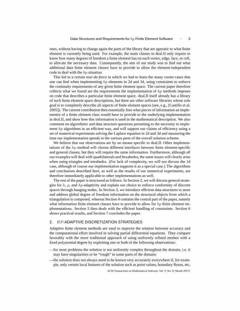
Fig. 2. Degrees of freedom onh- andp-adaptive meshes. Left: Dots indicate degrees of freedom for P1 (linear)elements on a mesh with a hanging node. Center: Resolution ofthe hanging node through introduction oftransition cells. Right: A mixture ofP1 andP3 elements on the original mesh.
a transition cell using strategies such asred-green refinement[Carey 1997], as shown inthe right panel of the figure. (An alternative strategy is to use Rivara’s algorithm [Rivara1984].) The left and center panel of Fig. 2 show the locationsof degrees of freedom forthese two cases for the commonP1 element with linear shape functions.
For pureh-refinement, both approaches have their merits, though we choose the first. Ifwe use piecewise linear shape functions in the depicted situation, continuity of the finiteelement functions requires that the value associated with the hanging node is equal to theaverage of the value at the two adjacent vertices along the unrefined side of the interface.We will explain this in more detail in Section 4.4.
2.2 p-adaptivity
In thep version of adaptivity, we keep the mesh constant but change the polynomial degreesof shape functions associated with each cell. The right panel of Fig. 2 shows this for thesituation that the rightmost cell of the original mesh is associated with aP3 (cubic) element,whereas the other elements still use linear elements.
As is seen from the figure, we again have two “hanging nodes” inthe form of the twoP3 degrees of freedom associated with the edge separating the two cells. There are againtwo widely used strategies to deal with this situation: introduction of constraints for thehanging nodes (explained in more detail in Section 4.3), andadding or removing degreesof freedom from one of the two adjacent cells. In the latter case, one would, for example,not use the fullP3 space on the rightmost cell, but use a reduced space that is missing thetwo shape functions associated with the line, and uses modified shape functions for thedegrees of freedom associated with the vertices of the common face. Alternatively, onecould use the fullP3 space on the rightmost cell, and augment the finite element space ofthe middle cell by the twoP3 shape functions defined on the common face.
2.3 hp-adaptivity
Thehp version of adaptivity combines both of the approaches discussed in the previoussubsections. One quickly realizes that the use of transition elements is not usually possibleto avoid hanging nodes in this case, and that the only optionsare, again, constraints orenriched/reduced finite element spaces on the adjacent cells.
As above, in our approach we opt to use constraints to deal with hanging nodes. This isnot to say that the alternative is not possible: it has in factbeen successfully implementedin numerical codes, see for example [Demkowicz 2006]. However, it is our feeling thatour approach is simpler in many ways: finite element codes almost always do operationssuch as integrating stiffness matrices and right hand side vectors on a cell-by-cell basis.
ACM Transactions on Mathematical Software, Vol. V, No. N, Month 20YY.
6 · W. Bangerth and O. Kayser-Herold
It is therefore advantageous if there is a simple description of the finite element spaceassociated with each cell. When using constraints, it is unequivocally clear that a cell is, forexample, associated with aP1, P2, orP3 finite element space and there is typically a fairlysmall number (for example less than 10) of possible spaces. On the other hand, there is aproliferation of spaces when enriching or reducing finite element spaces to avoid hangingnodes. This is especially true in 3-d, where each of the four neighbors of a tetrahedron mayor may not be refined, may or may not have a different space associated with it, etc. Tomake things worse, in 3-d not only the space associated with neighbor cells has to be takeninto account, but also the spaces associated with any of the potentially large number of cellsthat only share a single edge with the present cell. If one considers the case of problemswith several solution variables, one may want to use spacesPk1 × Pk2 × · · · × PkL
withdifferent indiceskl for each solution variable, and vary the indiceskl from cell to cell. Inthat case, the number of different enriched or reduced spaces becomes truly astronomicaland may easily lead to inefficient and/or unmaintainable code.
Given this reasoning, we opt to use constraints to deal with hanging nodes. The follow-ing sections will discuss algorithms and data structures tostore, generate, and use theseconstraints efficiently. Despite the relative simplicity of this approach, it should be notedalready at this place that the generation of constraints is not always straightforward andthat certain pathological cases exist, in particular in 3-d. However, we will enumerate andpresent solutions to all the cases we could find in our extensive use and testing of ourimplementation.
3. STORING GLOBAL INDICES OF DEGREES OF FREEDOM
In order to keep our implementation as general as can be achieved without unduly sacrific-ing performance, we have chosen to separate the concept of aDoFHandler from that ofa triangulation and a finite element class in deal.II (see [Bangerth et al. 2007] for more de-tails about this). ADoFHandler is a class that takes a triangulation and annotates it withglobal indices of the degrees of freedom associated with each of the cells, faces, edgesand vertices of the triangulation. ADoFHandler object is therefore independent of atriangulation object, and severalDoFHandler objects can be associated with the sametriangulation, for example to allow programs that use different discretizations on the samemesh.
On the other hand, aDoFHandler object is also independent of the concept of a globalfinite element space, since it doesn’t know anything about shape functions. It does, how-ever, draw information from one or several finite element objects (that implement shapefunctions) in that it needs to know how many degrees of freedom there are per vertex,line, etc. ADoFHandler is therefore associated with a triangulation and a finite elementobject and sets up a global enumeration of all degrees of freedom on the triangulation ascalled for by the finite element object.
The deal.II library has several implementations ofDoFHandler classes. The simplest,dealii::DoFHandler allocates degrees of freedom on a triangulation for the casethatall cells use the same finite element; on the contrary, thedealii::MGDoFHandlerclass allocates degrees of freedom for a multilevel hierarchy of finite element spaces. Inthe context of this paper, we are interested in the data structures necessary to implementhp finite element spaces, i.e. we have to deal with the situationthat different cells might beassociated with different (local) finite element spaces. This concept is implemented in the
ACM Transactions on Mathematical Software, Vol. V, No. N, Month 20YY.

Data Structures and Requirements for hp Finite Element Software · 7
v v v l l 4 5 2 3 3
v
l
v
l q
l
l
v
q
l 1 2 1 0
4 5 6
0
0 1
21
20
19
27
25
26
28
29
30 33
31
32
10
2
144
6
0 15
1816
13
5 17 12
7
22
23
24
8
91
3 11
Fig. 3. Left: A mesh consisting of two cells with a numbering of the vertices, lines, and quadrilaterals of thismesh. Right: A possible enumeration of degrees of freedom where the polynomial space on the left cell representsa Q2 element and that on the right cell aQ4 element. Bottom: Linked lists of degrees of freedom on each of theobjects of which the triangulation consists.
classdealii::hp::DoFHandler.2
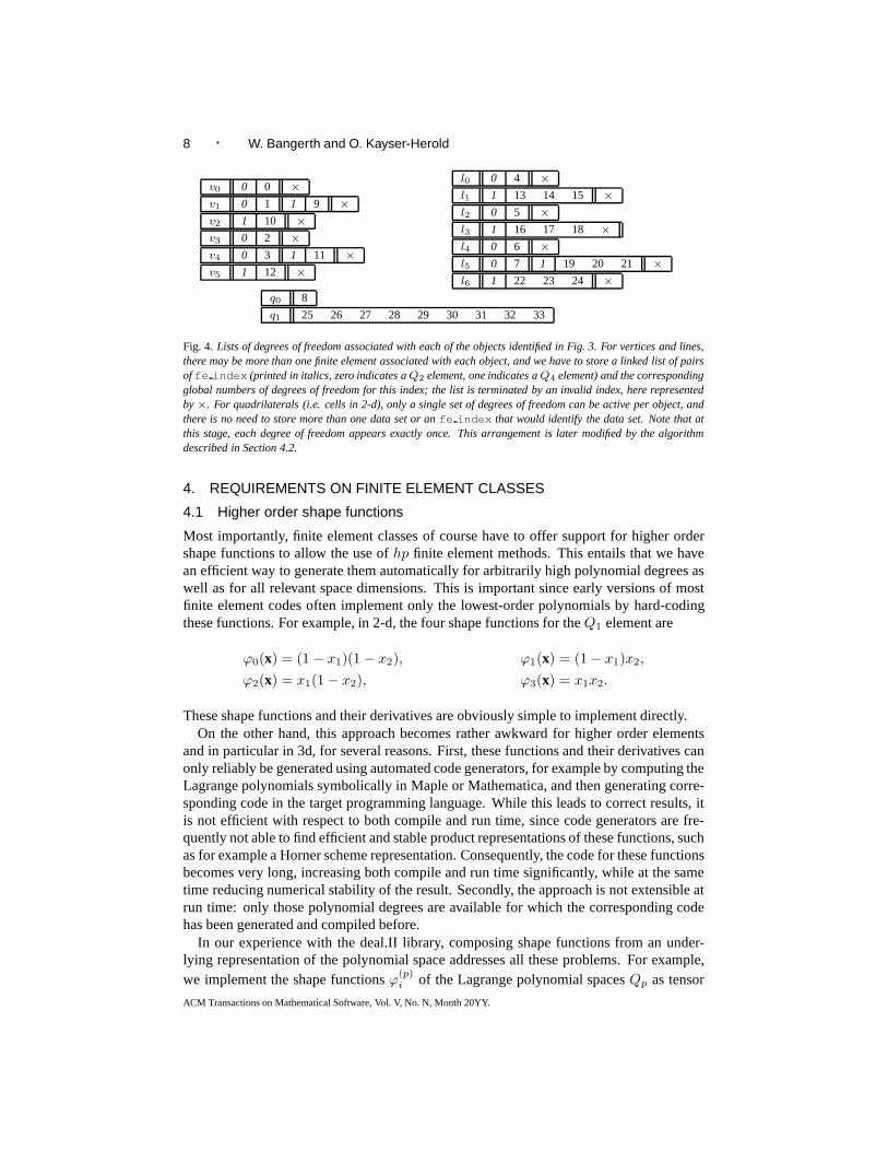
Clearly, each cell is only associated with a single finite element, and only a single setof degrees of freedom has to be stored for each cell. However,the lower-dimensionalobjects (vertices, lines, and faces) that encircle a cell may be associated with multiplesets of degrees of freedom. For example, consider the situation shown in Fig. 3. There,a quadraticQ2 element is associated with the left cell, whereas a quarticQ4 element isassociated with the one on the right. Here, the vertices v1 and v4 as well as the line l5 areall associated with both local finite element spaces. We therefore have to store the globalindices of the degrees of freedom associated with both spaces for these objects.
Furthermore, it is clear that vertices in 2-d, and lines in 3-d, may be associated with asmany finite element spaces as there are cells that meet at thisvertex or line. This leads toour first requirement on implementations:
REQUIREMENT ON IMPLEMENTATIONS 1. An implementation needs to store the globalindices of degrees of freedom associated with each object (vertices, lines, etc.) of a trian-gulation. This storage scheme must be efficient both in termsof memory and in terms offast access.
Note that we only store the indices of degrees of freedom, notdata associated with it.However, the indices can be used to look up data values in vectors and matrices.
In deal.II, we implement above requirement in thehp::DoFHandler class using asort of linked list that is attached to each object of a triangulation. This list consists ofone record for each finite element associated with this object, where a record consists ofthe number of the finite element as well as the global indices that belong to it. This isillustrated in Fig. 4 where we show these linked lists for each of the objects found in thetriangulation depicted in Fig. 3. The caption also containsfurther explanations about thedata format.
While other implementations are clearly possible, note that this storage scheme mini-mizes memory fragmentation. Furthermore, because in the vast majority of cases only asingle element is associated with an object, access is also very fast since the linked listcontains only one record.
2To avoid redundancy, we will drop the namespace prefixdealii:: from here on.
ACM Transactions on Mathematical Software, Vol. V, No. N, Month 20YY.
8 · W. Bangerth and O. Kayser-Herold
v0 0 0 ×
v1 0 1 1 9 ×
v2 1 10 ×
v3 0 2 ×
v4 0 3 1 11 ×
v5 1 12 ×
l0 0 4 ×
l1 1 13 14 15 ×
l2 0 5 ×
l3 1 16 17 18 ×
l4 0 6 ×
l5 0 7 1 19 20 21 ×
l6 1 22 23 24 ×
q0 8
q1 25 26 27 28 29 30 31 32 33
Fig. 4. Lists of degrees of freedom associated with each of the objects identified in Fig. 3. For vertices and lines,there may be more than one finite element associated with eachobject, and we have to store a linked list of pairsoffe index (printed in italics, zero indicates aQ2 element, one indicates aQ4 element) and the correspondingglobal numbers of degrees of freedom for this index; the listis terminated by an invalid index, here representedby×. For quadrilaterals (i.e. cells in 2-d), only a single set ofdegrees of freedom can be active per object, andthere is no need to store more than one data set or anfe index that would identify the data set. Note that atthis stage, each degree of freedom appears exactly once. This arrangement is later modified by the algorithmdescribed in Section 4.2.
4. REQUIREMENTS ON FINITE ELEMENT CLASSES
4.1 Higher order shape functions
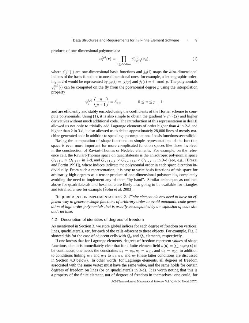
Most importantly, finite element classes of course have to offer support for higher ordershape functions to allow the use ofhp finite element methods. This entails that we havean efficient way to generate them automatically for arbitrarily high polynomial degrees aswell as for all relevant space dimensions. This is importantsince early versions of mostfinite element codes often implement only the lowest-order polynomials by hard-codingthese functions. For example, in 2-d, the four shape functions for theQ1 element are
ϕ0(x) = (1 − x1)(1 − x2), ϕ1(x) = (1 − x1)x2,
ϕ2(x) = x1(1 − x2), ϕ3(x) = x1x2.
These shape functions and their derivatives are obviously simple to implement directly.On the other hand, this approach becomes rather awkward for higher order elements
and in particular in 3d, for several reasons. First, these functions and their derivatives canonly reliably be generated using automated code generators, for example by computing theLagrange polynomials symbolically in Maple or Mathematica, and then generating corre-sponding code in the target programming language. While this leads to correct results, itis not efficient with respect to both compile and run time, since code generators are fre-quently not able to find efficient and stable product representations of these functions, suchas for example a Horner scheme representation. Consequently, the code for these functionsbecomes very long, increasing both compile and run time significantly, while at the sametime reducing numerical stability of the result. Secondly,the approach is not extensible atrun time: only those polynomial degrees are available for which the corresponding codehas been generated and compiled before.
In our experience with the deal.II library, composing shapefunctions from an under-lying representation of the polynomial space addresses allthese problems. For example,we implement the shape functionsϕ(p)
i of the Lagrange polynomial spacesQp as tensor
ACM Transactions on Mathematical Software, Vol. V, No. N, Month 20YY.
Data Structures and Requirements for hp Finite Element Software · 9
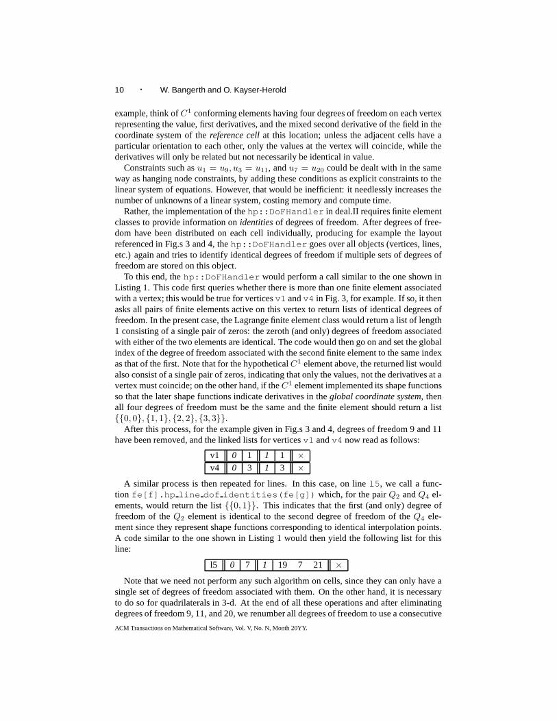
products of one-dimensional polynomials:
ϕ(p)i (x) =
∏
0≤d<dim
ψ(p)jd(i)(xd), (1)
whereψ(p)j (·) are one-dimensional basis functions andjd(i) maps thedim-dimensional
indices of the basis functions to one-dimensional ones; forexample, a lexicographic order-ing in 2-d would be represented byj0(i) = ⌊i/p⌋ andj1(i) = i mod p. The polynomials
ψ(p)j (·) can be computed on the fly from the polynomial degreep using the interpolation
property
ψ(p)j
(
n
p+ 1
)
= δnj, 0 ≤ n ≤ p+ 1,
and are efficiently and stably encoded using the coefficientsof the Horner scheme to com-pute polynomials. Using (1), it is also simple to obtain the gradient∇ψ(p)(x) and higherderivatives without much additional code. The introduction of this representation in deal.IIallowed us not only to trivially add Lagrange elements of order higher than 4 in 2-d andhigher than 2 in 3-d, it also allowed us to delete approximately 28,000 lines of mostly ma-chine generated code in addition to speeding up computationof basis functions severalfold.
Basing the computation of shape functions on simple representations of the functionspace is even more important for more complicated function spaces like those involvedin the construction of Raviart-Thomas or Nedelec elements.For example, on the refer-ence cell, the Raviart-Thomas space on quadrilaterals is the anisotropic polynomial spaceQk+1,k × Qk,k+1 in 2-d, andQk+1,k,k × Qk,k+1,k × Qk,k,k+1 in 3-d (see, e.g., [Brezziand Fortin 1991]), where indices indicate the polynomial order in each space direction in-dividually. From such a representation, it is easy to write basis functions of this space forarbitrarily high degrees as a tensor product of one-dimensional polynomials, completelyavoiding the need to implement any of them “by hand”. Similartechniques as outlinedabove for quadrilaterals and hexahedra are likely also going to be available for trianglesand tetrahedra, see for example [Solın et al. 2003].
REQUIREMENT ON IMPLEMENTATIONS 2. Finite element classes need to have an ef-ficient way to generate shape functions of arbitrary order toavoid automatic code gener-ation of high order polynomials that is usually accompaniedby an explosion of code sizeand run time.
4.2 Description of identities of degrees of freedom
As mentioned in Section 3, we store global indices for each degree of freedom on vertices,lines, quadrilaterals, etc, for each of the cells adjacent to these objects. For example, Fig. 3showed this for the case of adjacent cells withQ2 andQ4 elements, respectively.
If one knows that for Lagrange elements, degrees of freedom representvaluesof shapefunctions, then it is immediately clear that for a finite element fieldu(x) =
∑
i uiϕi(x) tobe continuous, one needs the constraintsu1 = u9, u3 = u11, andu7 = u20, in additionto conditions linkingu19 andu21 to u1, u3, andu7 (these latter conditions are discussedin Section 4.3 below). In other words, for Lagrange elements, all degrees of freedomassociated with the same vertex must have the same value, andthe same holds for certaindegrees of freedom on lines (or on quadrilaterals in 3-d). Itis worth noting that this isa property of the finite element, not of degrees of freedom in themselves: one could, for
ACM Transactions on Mathematical Software, Vol. V, No. N, Month 20YY.
10 · W. Bangerth and O. Kayser-Herold
example, think ofC1 conforming elements having four degrees of freedom on each vertexrepresenting the value, first derivatives, and the mixed second derivative of the field in thecoordinate system of thereference cellat this location; unless the adjacent cells have aparticular orientation to each other, only the values at thevertex will coincide, while thederivatives will only be related but not necessarily be identical in value.
Constraints such asu1 = u9, u3 = u11, andu7 = u20 could be dealt with in the sameway as hanging node constraints, by adding these conditionsas explicit constraints to thelinear system of equations. However, that would be inefficient: it needlessly increases thenumber of unknowns of a linear system, costing memory and compute time.
Rather, the implementation of thehp::DoFHandler in deal.II requires finite elementclasses to provide information onidentitiesof degrees of freedom. After degrees of free-dom have been distributed on each cell individually, producing for example the layoutreferenced in Fig.s 3 and 4, thehp::DoFHandler goes over all objects (vertices, lines,etc.) again and tries to identify identical degrees of freedom if multiple sets of degrees offreedom are stored on this object.
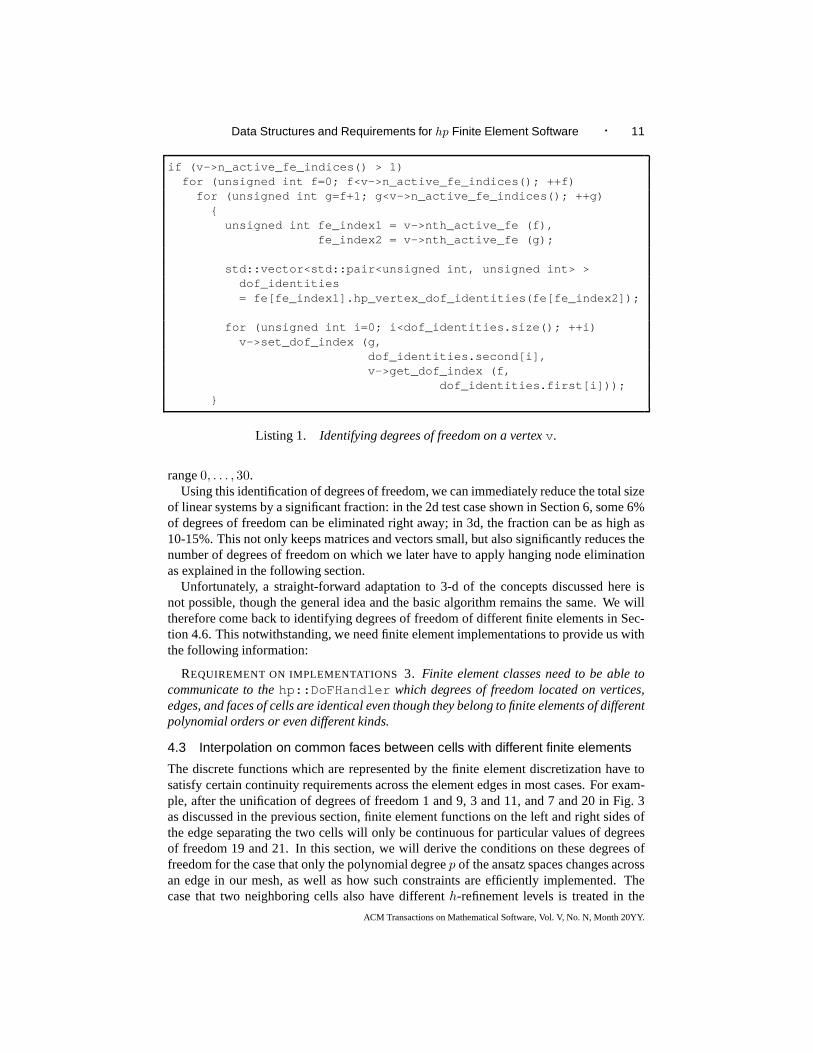
To this end, thehp::DoFHandler would perform a call similar to the one shown inListing 1. This code first queries whether there is more than one finite element associatedwith a vertex; this would be true for verticesv1 andv4 in Fig. 3, for example. If so, it thenasks all pairs of finite elements active on this vertex to return lists of identical degrees offreedom. In the present case, the Lagrange finite element class would return a list of length1 consisting of a single pair of zeros: the zeroth (and only) degrees of freedom associatedwith either of the two elements are identical. The code wouldthen go on and set the globalindex of the degree of freedom associated with the second finite element to the same indexas that of the first. Note that for the hypotheticalC1 element above, the returned list wouldalso consist of a single pair of zeros, indicating that only the values, not the derivatives at avertex must coincide; on the other hand, if theC1 element implemented its shape functionsso that the later shape functions indicate derivatives in the global coordinate system, thenall four degrees of freedom must be the same and the finite element should return a list0, 0, 1, 1, 2, 2, 3, 3.
After this process, for the example given in Fig.s 3 and 4, degrees of freedom 9 and 11have been removed, and the linked lists for verticesv1 andv4 now read as follows:
v1 0 1 1 1 ×
v4 0 3 1 3 ×
A similar process is then repeated for lines. In this case, online l5, we call a func-tion fe[f].hp line dof identities(fe[g]) which, for the pairQ2 andQ4 el-ements, would return the list0, 1. This indicates that the first (and only) degree offreedom of theQ2 element is identical to the second degree of freedom of theQ4 ele-ment since they represent shape functions corresponding toidentical interpolation points.A code similar to the one shown in Listing 1 would then yield the following list for thisline:
l5 0 7 1 19 7 21 ×
Note that we need not perform any such algorithm on cells, since they can only have asingle set of degrees of freedom associated with them. On theother hand, it is necessaryto do so for quadrilaterals in 3-d. At the end of all these operations and after eliminatingdegrees of freedom 9, 11, and 20, we renumber all degrees of freedom to use a consecutive
ACM Transactions on Mathematical Software, Vol. V, No. N, Month 20YY.
Data Structures and Requirements for hp Finite Element Software · 11
if (v->n_active_fe_indices() > 1)for (unsigned int f=0; f<v->n_active_fe_indices(); ++f)for (unsigned int g=f+1; g<v->n_active_fe_indices(); ++g)
unsigned int fe_index1 = v->nth_active_fe (f),
fe_index2 = v->nth_active_fe (g);
std::vector<std::pair<unsigned int, unsigned int> >dof_identities= fe[fe_index1].hp_vertex_dof_identities(fe[fe_index2]);
for (unsigned int i=0; i<dof_identities.size(); ++i)v->set_dof_index (g,
dof_identities.second[i],v->get_dof_index (f,
dof_identities.first[i]));
Listing 1. Identifying degrees of freedom on a vertexv.
range0, . . . , 30.Using this identification of degrees of freedom, we can immediately reduce the total size
of linear systems by a significant fraction: in the 2d test case shown in Section 6, some 6%of degrees of freedom can be eliminated right away; in 3d, thefraction can be as high as10-15%. This not only keeps matrices and vectors small, but also significantly reduces thenumber of degrees of freedom on which we later have to apply hanging node eliminationas explained in the following section.
Unfortunately, a straight-forward adaptation to 3-d of theconcepts discussed here isnot possible, though the general idea and the basic algorithm remains the same. We willtherefore come back to identifying degrees of freedom of different finite elements in Sec-tion 4.6. This notwithstanding, we need finite element implementations to provide us withthe following information:
REQUIREMENT ON IMPLEMENTATIONS 3. Finite element classes need to be able tocommunicate to thehp::DoFHandler which degrees of freedom located on vertices,edges, and faces of cells are identical even though they belong to finite elements of differentpolynomial orders or even different kinds.
4.3 Interpolation on common faces between cells with different finite elements
The discrete functions which are represented by the finite element discretization have tosatisfy certain continuity requirements across the element edges in most cases. For exam-ple, after the unification of degrees of freedom 1 and 9, 3 and 11, and 7 and 20 in Fig. 3as discussed in the previous section, finite element functions on the left and right sides ofthe edge separating the two cells will only be continuous forparticular values of degreesof freedom 19 and 21. In this section, we will derive the conditions on these degrees offreedom for the case that only the polynomial degreep of the ansatz spaces changes acrossan edge in our mesh, as well as how such constraints are efficiently implemented. Thecase that two neighboring cells also have differenth-refinement levels is treated in the
ACM Transactions on Mathematical Software, Vol. V, No. N, Month 20YY.
12 · W. Bangerth and O. Kayser-Herold
next sections. In the presentation of these techniques, we follow to some degree the algo-rithms shown in [Ainsworth and Senior 1997; 1999]; however,we go beyond the materialpresented there in that we allow for the case of local refinement where thecoarsercellhas a higher polynomial degree, and in that we discuss some complications specific to thethree-dimensional case.
It is worth noting that continuity requirements do not always enforce that a function hasto be continuous across element edges. For example, discrete subspaces ofH(div) onlyrequire continuity of the normal component along the faces between cells (c.f. [Brezzi andFortin 1991]). For the sake of simplicity, let us here only consider continuity of functionsacross element edges; it shall be understood that the same requirements and assumptionsalso hold when the normal or tangential component has to be continuous along elementedges.
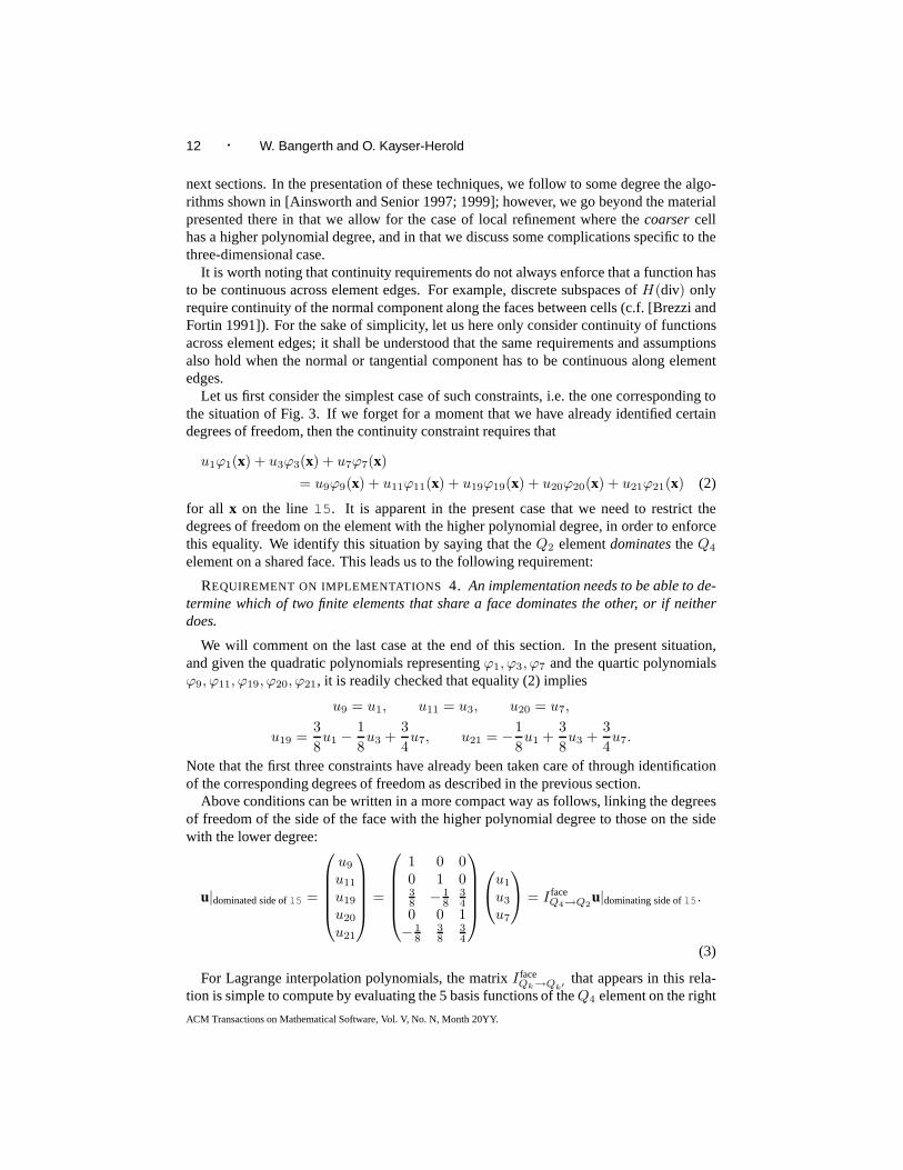
Let us first consider the simplest case of such constraints, i.e. the one corresponding tothe situation of Fig. 3. If we forget for a moment that we have already identified certaindegrees of freedom, then the continuity constraint requires that
u1ϕ1(x) + u3ϕ3(x) + u7ϕ7(x)
= u9ϕ9(x) + u11ϕ11(x) + u19ϕ19(x) + u20ϕ20(x) + u21ϕ21(x) (2)
for all x on the linel5. It is apparent in the present case that we need to restrict thedegrees of freedom on the element with the higher polynomialdegree, in order to enforcethis equality. We identify this situation by saying that theQ2 elementdominatestheQ4
element on a shared face. This leads us to the following requirement:
REQUIREMENT ON IMPLEMENTATIONS 4. An implementation needs to be able to de-termine which of two finite elements that share a face dominates the other, or if neitherdoes.
We will comment on the last case at the end of this section. In the present situation,and given the quadratic polynomials representingϕ1, ϕ3, ϕ7 and the quartic polynomialsϕ9, ϕ11, ϕ19, ϕ20, ϕ21, it is readily checked that equality (2) implies
u9 = u1, u11 = u3, u20 = u7,
u19 =3
8u1 −
1
8u3 +
3
4u7, u21 = −
1
8u1 +
3
8u3 +
3
4u7.
Note that the first three constraints have already been takencare of through identificationof the corresponding degrees of freedom as described in the previous section.
Above conditions can be written in a more compact way as follows, linking the degreesof freedom of the side of the face with the higher polynomial degree to those on the sidewith the lower degree:
u|dominated side ofl5 =
u9
u11
u19
u20
u21
=
1 0 00 1 038 − 1
834
0 0 1− 1
838
34
u1
u3
u7
= I faceQ4→Q2
u|dominating side ofl5.
(3)
For Lagrange interpolation polynomials, the matrixI faceQk→Qk′
that appears in this rela-tion is simple to compute by evaluating the 5 basis functionsof theQ4 element on the right
ACM Transactions on Mathematical Software, Vol. V, No. N, Month 20YY.
Data Structures and Requirements for hp Finite Element Software · 13
at the interpolation points of the 3 basis functions of theQ2 element on the left. However,these matrices are more complicated to compute for elementswhere the degrees of free-dom are moments on faces or where values and not only gradients of shape functions aretransformed by the mapping from reference to real cell; boththese cases apply to elementssuch as the Raviart-Thomas element forH(div).
REQUIREMENT ON IMPLEMENTATIONS 5. Finite element classes need to be able togenerate the constraint matricesI face as in (3) that enforce continuity requirements be-tween cells associated with different finite element spaces. These matrices must be avail-able for all possible pairs of spaces appearing in a triangulation.
We remark that an important requirement for this approach isthat the functions appear-ing on one side of (2) must be able to exactly represent the functions on the other side.For the chosen pair of spaces, this is obvious: the restriction ofQ4 onto a line is the spaceof quartic polynomials that is of course able to represent the quadratic polynomials thatresult from restrictingQ2 to this line, i.e. we say that theQ2 elementsdominatestheQ4
element. However, it is not always the case that one element dominates the other. Forexample, consider the hypothetical situation of a mesh containing an edge where elementsmeet that haveQ4 andR2,2 (the space of rational expressions with quadratic denominatorand enumerator) elements: neither of the two is able to represent the restriction of the otherone on a common edge, i.e. neither element dominates the other. Another, more practicalexample, would be that one cell is home to aQ2 ×Q1 vector-valued element, whereas itsneighbor is associated with aQ1 ×Q2 element.
The solution to this case is to first identify a common subspace; in the first examplethis could be the spaceQ2 of quadratic polynomials on this face, whereas in the secondwe would chooseQ1 × Q1. The second step would then be to enforce constraints thatrestrict finite element functions on both sides of the face tobe within this subspace, and inaddition to be equal along the face. In order to not restrict the global finite element spacemore than necessary, we should attempt to find the largest admissible subspace along theface. However, since this is a case that doesn’t appear to have much application in practicalfinite element cases, we won’t dwell on it in more detail, but will come back to a closelyrelated case in Section 4.4.3.
4.4 Interpolation on refined faces between cells
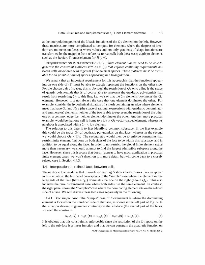
The next case to consider is that ofh-refinement. Fig. 5 shows the two cases that can appearin this situation: the left panel corresponds to the “simple” case where the element on thelarge side of the face (here aQ1) dominates the one on the right (here aQ2). This alsoincludes the pureh-refinement case where both sides use the same element. In contrast,the right panel shows the “complex” case where the dominating element sits on the refinedside of a face. We will discuss these two cases separately in the following.
4.4.1 The simple case.The “simple” case ofh-refinement is where the dominatingelement is located on the unrefined side of the face, as shown in the left part of Fig. 5. Inthe situation shown, to guarantee continuity at the sub-face (the shared part of the face),we need the constraint
u0ϕ0(x) + u1ϕ1(x) = u2ϕ2(x) + u3ϕ3(x) + u4ϕ4(x). (4)
It is obvious that this constraint is enforceable since the restriction of theQ1 space on theleft to the sub-face is a linear function and that we can constrain the quadratic function on
ACM Transactions on Mathematical Software, Vol. V, No. N, Month 20YY.

14 · W. Bangerth and O. Kayser-Herold
0
1
2
34
Q1
Q2
0
1 4
Q2
Q13
Q35
6
78
2
Fig. 5. The simple (left) and complicated (right) case ofh-refinement across a face between cells with differentfinite element spaces associated with them. Only those degrees of freedom that are relevant for the interpolationprocess are indicated.
the right to equal this linear function. In particular, it iseasy to show that we need
u|dominated side of subface=
u2
u3
u4
=
12
12
0 114 − 3
4
(
u0
u1
)
= Isubface(sf)Q2→Q1
u|dominating side of subface,
(5)
wheresf denotes the number of the subface we are presently looking at. As before, forQk elements, we can obtain the interpolation matrixIsubface(sf) by evaluating the shapefunctions associated with the coarse side of the face at the interpolation points of the shapefunctions on the refined side of the face.
REQUIREMENT ON IMPLEMENTATIONS 6. Finite element classes need to be able togenerate the constraint matricesIsubface(sf) as in (5), for each of the2dim−1 subfacessf ofa face. These matrices must be available for all possible pairs of spaces appearing in atriangulation.
In deal.II, this requirement is currently implemented for elements from the same familyby automatically computing the interpolation matrices at interfaces between cells.
4.4.2 The complex case, approach 1.The more complicated case is the one shownon the right of Fig. 5. The problem is that the linear (dominating) element is located onthe refined side of the subface. As we will see in the following, this case is riddled withproblems, false hopes, and traps; we will consider several cases and possible solutions thatillustrate why this case is hard.
A naive approach to the situation shown in Fig. 5 is as follows: In order to force conti-nuity of finite element functions, we need to make sure that the three degrees of freedom0, 1, and 2 of theQ2 element actually form a linear function, since otherwise there wouldbe no way the linear function on the upper rightQ1 cell could match the one on the left.In general, we need to constrain the finite element space on the left of the refined face tothe most dominating space on the right, hereQ1. We could do that by constraining the leftface to the degrees of freedom 3 and 4 of the most dominating child face, i.e. to require
u|dominated side of face=
u0
u1
u2
=
2 −10 11 0
(
u3
u4
)
= RIsubface(sf)Q1→Q2
u|most dominating subface.
We call the matrixRIsubface(sf)Q1→Q2
the reverse interpolation matrix. It is not hard to see that
ACM Transactions on Mathematical Software, Vol. V, No. N, Month 20YY.
Data Structures and Requirements for hp Finite Element Software · 15
for this particular subface, we can write it as
RIsubface(sf)Q1→Q2
= I faceQ2→Q1
[
Isubface(sf)Q1→Q1
]−1
=
1 00 112
12
(
12
12
0 1
)−1
. (6)
This formula can be understood as follows: Let us introduce the degrees of freedomx0, x1
of a virtual linear finite element space along the entire edge. The condition of continuitythen means that
u0
u1
u2
= I faceQ2→Q1
(
x0
x1
)
,
(
u3
u4
)
= Isubface(sf)Q1→Q1
(
x0
x1
)
.
It is now important to realize that the matrixIsubface(sf)Q1→Q1
should always be invertible, evenif we replace the spaceQ1 by any other reasonable finite element space. This followsfrom the fact that the matrix intuitively describes how a finite element space on a face isrestricted to the same space but on a subface. Its inverse, ifit exists, then describes howa finite element function on a subface uniquely determines the function on the entire face.Since we are dealing with polynomials, the existence and uniqueness of the inverse is easyto see: polynomials are analytic functions, and its Taylor expansion on a subface thereforeuniquely determines its extension to the entire face. The matrix that relates the values ofthis polynomial at disjoint interpolation points must consequently be invertible.
Given this, (6) is therefore a universal representation of the reverse interpolation matrixthat we can obtain by removing the virtual unknownsx0, x1 from the equations.
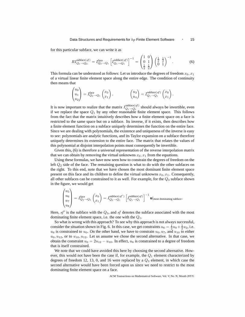
Using these formulas, we have now seen how to constrain the degrees of freedom on theleft Q2 side of the face. The remaining question is what to do with theother subfaces onthe right. To this end, note that we have chosen the most dominant finite element spacepresent on this face and its children to define the virtual unknownsx0, x1. Consequently,all other subfaces can be constrained to it as well. For example, for theQ3 subface shownin the figure, we would get
u5
u6
u7
u8
= I faceQ3→Q1
(
x0
x1
)
= Isubface(sf ′)Q3→Q1
[
Isubface(sf)Q1→Q1
]−1
u|most dominating subface.
Here,sf ′ is the subface with theQ3, andsf denotes the subface associated with the mostdominating finite element space, i.e. the one with theQ1.
So what is wrong with this approach? To see why this approach is not always successful,consider the situation shown in Fig. 6. In this case, we get constraintsu6 = 1
2u0+ 12u2, i.e.
u6 is constrained tou0. On the other hand, we have to constrainu0, u7, andu10 to eitheru0, u12, or to u10, u12. Let us assume we chose the second alternative. In that case,weobtain the constraintu0 = 2u12 − u10. In effect,u6 is constrained to a degree of freedomthat is itself constrained.
We note that we could have avoided this here by choosing the second alternative. How-ever, this would not have been the case if, for example, theQ1 element characterized bydegrees of freedom 12, 13, 0, and 16 were replaced by aQ3 element, in which case thesecond alternative would have been forced upon us since we need to restrict to the mostdominating finite element space on a face.
ACM Transactions on Mathematical Software, Vol. V, No. N, Month 20YY.
16 · W. Bangerth and O. Kayser-Herold
Q2
Q1
Q1 Q1
Q1
Q1
4
10 14
15
1
32
0
16
1312
5
96
8
11
7
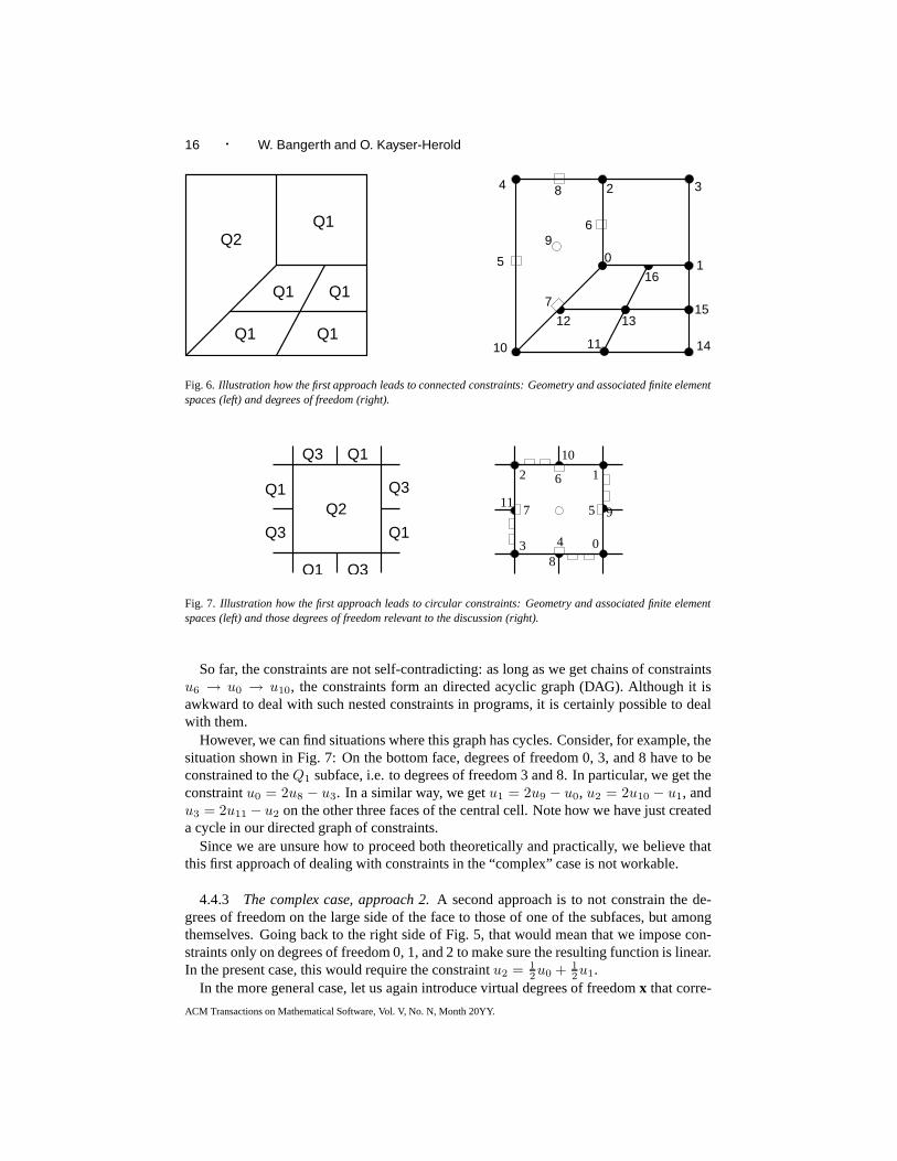
Fig. 6. Illustration how the first approach leads to connected constraints: Geometry and associated finite elementspaces (left) and degrees of freedom (right).
Q2
Q3
Q3
Q3
Q3
Q1
Q1
Q1
Q19
8
10
11
4 03
2 16
57
Fig. 7. Illustration how the first approach leads to circular constraints: Geometry and associated finite elementspaces (left) and those degrees of freedom relevant to the discussion (right).
So far, the constraints are not self-contradicting: as longas we get chains of constraintsu6 → u0 → u10, the constraints form an directed acyclic graph (DAG). Although it isawkward to deal with such nested constraints in programs, itis certainly possible to dealwith them.
However, we can find situations where this graph has cycles. Consider, for example, thesituation shown in Fig. 7: On the bottom face, degrees of freedom 0, 3, and 8 have to beconstrained to theQ1 subface, i.e. to degrees of freedom 3 and 8. In particular, weget theconstraintu0 = 2u8 − u3. In a similar way, we getu1 = 2u9 − u0, u2 = 2u10 − u1, andu3 = 2u11 − u2 on the other three faces of the central cell. Note how we have just createda cycle in our directed graph of constraints.
Since we are unsure how to proceed both theoretically and practically, we believe thatthis first approach of dealing with constraints in the “complex” case is not workable.
4.4.3 The complex case, approach 2.A second approach is to not constrain the de-grees of freedom on the large side of the face to those of one ofthe subfaces, but amongthemselves. Going back to the right side of Fig. 5, that wouldmean that we impose con-straints only on degrees of freedom 0, 1, and 2 to make sure theresulting function is linear.In the present case, this would require the constraintu2 = 1
2u0 + 12u1.
In the more general case, let us again introduce virtual degrees of freedomx that corre-
ACM Transactions on Mathematical Software, Vol. V, No. N, Month 20YY.
Data Structures and Requirements for hp Finite Element Software · 17
spond to the most dominant finite element restricted to a face, which we nameS. Then
u|coarse side of face= I faceSface→Sx,
whereS face is the finite element space on the coarse side of the face. Since we haveassumed thatS face is dominated byS, we can divideu|coarse side of faceinto a set of masterand slave nodes such that
u|coarse side of face=
(
u|mastercoarse side of face
u|slavecoarse side of face
)
=
(
I face, masterSface→S
I face, slaveSface→S
)
x.
Let us assume that we can subdivide degrees of freedom into master and slave nodes suchthat I face, master
Sface→Sis an invertible square matrix (an assumption that we will discuss below),
then we can conclude that
u|slavecoarse side of face= I face, slave
Sface→Sx = I face, slave
Sface→S
[
I face, masterSface→S
]−1
u|mastercoarse side of face.
Now that we know how to deal with the degrees of freedom on the coarse side of theface, it is clear that we can deal with the subfaces as follows:
u|subfacesf = Isubface(sf)
Ssubface(sf)→Sx = I
subface(sf)
Ssubface(sf)→S
[
I face, masterSface→S
]−1
u|mastercoarse side of face.
Here,Ssubface(sf) is the finite element space on subfacesf .Using this second approach, one can easily construct situations where one gets chains
of constraints. For example, theQ3 degrees of freedom on the interface between the smallQ1 andQ3 cells at the bottom of Fig. 7 (though not explicitly shown) will be constrainedto the degrees of freedom located on the two vertices of the common edge. One of those isdegree of freedom 8, which is itself constrained to degrees of freedom 0 and 3.
However, it is easy to prove that with this second approach there can be no cycles in thegraph of constraints: resulting from the definition of dominance of spaces, each constraintis always from a degree of freedom to other ones associated with a strictly smaller embed-ded finite element space. The fact that this wasn’t the case for the first approach illustratesimmediately why that approach was prone to failure.
We conclude this subsection with a discussion of the slight complication of how tochoose the subdivision of nodes on the coarse side of the faceinto master and slave nodes,u|master
coarse side of faceandu|slavecoarse side of face. First, let us note that the matrixI face
Sface→Snecessarily
must have full column rank, since it is the matrix that interpolates the shape functions ofthe dominating spaceS at the support points of the dominated spaceS face. AssumingS tobe unisolvent, i.e. consisting of linearly independent shape functions, and assuming that notwo interpolation points ofS face coincide, then the full column rank immediately follows.Consequently, we can hope that we can select certain linearly independent rows ofI face
Sface→S
to form an invertible matrixI face,masterSface→S
.The selection of these rows, however, turns out to be more involved than one would
think at first. In particular, one can not simply take the firstnS of thenSface rows, sincethey sometimes are linearly dependent. It is conceivable that one could devise an exactstrategy for this problem, though we are not aware of any suchapproach and thereforechose to implement a heuristic: ifnvertex
S , nlineS , nquad
S are the number of degrees of freedomassociated with each vertex, line, and quad of the dominating spaceS, then select the firstnvertex
S degrees of freedom from each vertex in the dominated spaceS face as master nodes,then the firstnline
S degrees of freedom from each line, and so on.
ACM Transactions on Mathematical Software, Vol. V, No. N, Month 20YY.
18 · W. Bangerth and O. Kayser-Herold
3
4
2
1
0
Q1
Q2Q3 6
5
2
3
42
1
0
Q2
Q4Q3
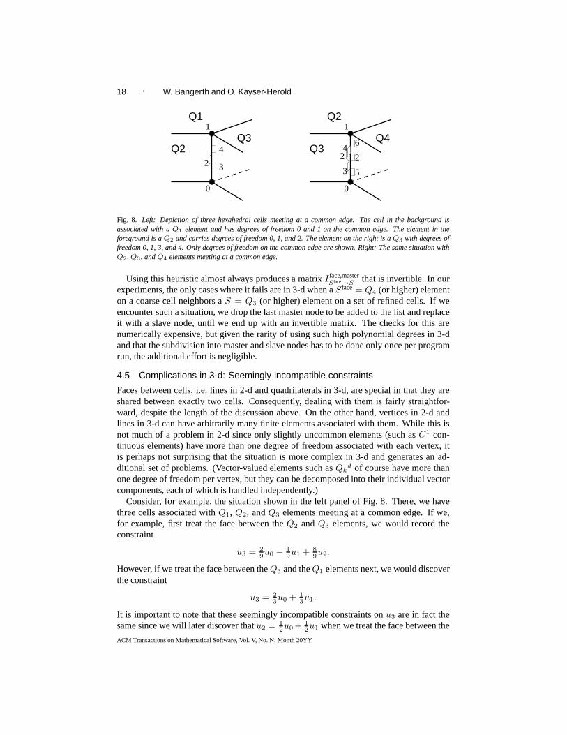
Fig. 8. Left: Depiction of three hexahedral cells meeting at a common edge. The cell in the background isassociated with aQ1 element and has degrees of freedom 0 and 1 on the common edge. The element in theforeground is aQ2 and carries degrees of freedom 0, 1, and 2. The element on the right is aQ3 with degrees offreedom 0, 1, 3, and 4. Only degrees of freedom on the common edge are shown. Right: The same situation withQ2, Q3, andQ4 elements meeting at a common edge.
Using this heuristic almost always produces a matrixI face,masterSface→S
that is invertible. In ourexperiments, the only cases where it fails are in 3-d when aS face = Q4 (or higher) elementon a coarse cell neighbors aS = Q3 (or higher) element on a set of refined cells. If weencounter such a situation, we drop the last master node to beadded to the list and replaceit with a slave node, until we end up with an invertible matrix. The checks for this arenumerically expensive, but given the rarity of using such high polynomial degrees in 3-dand that the subdivision into master and slave nodes has to bedone only once per programrun, the additional effort is negligible.
4.5 Complications in 3-d: Seemingly incompatible constraints
Faces between cells, i.e. lines in 2-d and quadrilaterals in3-d, are special in that they areshared between exactly two cells. Consequently, dealing with them is fairly straightfor-ward, despite the length of the discussion above. On the other hand, vertices in 2-d andlines in 3-d can have arbitrarily many finite elements associated with them. While this isnot much of a problem in 2-d since only slightly uncommon elements (such asC1 con-tinuous elements) have more than one degree of freedom associated with each vertex, itis perhaps not surprising that the situation is more complexin 3-d and generates an ad-ditional set of problems. (Vector-valued elements such asQk
d of course have more thanone degree of freedom per vertex, but they can be decomposed into their individual vectorcomponents, each of which is handled independently.)
Consider, for example, the situation shown in the left panelof Fig. 8. There, we havethree cells associated withQ1, Q2, andQ3 elements meeting at a common edge. If we,for example, first treat the face between theQ2 andQ3 elements, we would record theconstraint
u3 = 29u0 −
19u1 + 8
9u2.
However, if we treat the face between theQ3 and theQ1 elements next, we would discoverthe constraint
u3 = 23u0 + 1
3u1.
It is important to note that these seemingly incompatible constraints onu3 are in fact thesame since we will later discover thatu2 = 1
2u0 + 12u1 when we treat the face between the
ACM Transactions on Mathematical Software, Vol. V, No. N, Month 20YY.

Data Structures and Requirements for hp Finite Element Software · 19
Q2 andQ1 elements, and we can expand the first constraint onu3 into the second form byresolving the chain of constraints.
REQUIREMENT ON IMPLEMENTATIONS 7. An implementation has to be able to keeptrack which degrees of freedom are already constrained, andsimply ignore constraintsgenerated for degrees of freedom for which other constraints have already been registered.
While this is a simple solution, it is bothersome that one loses the ability for safetychecks by just throwing away a constraint. It would be nicer if we could keep it, expandthe constraint later on whenu2 is resolved, and then make sure that it equals the originalconstraint with which it appeared to conflict. A defensive implementation would thereforefollow this latter strategy, in order to ensure that our computations are correct, and producean error if the two constraints are not the same. We have foundthis strategy of perva-sive and exhaustive internal consistency checks of great value in finding obscure bugs andcorner cases in our implementation.
4.6 Complications in 3-d: Seemingly circular constraints
Yet another situation is shown in the right panel of Fig. 8. The situation is similar to theone discussed in the preceding subsection, but with polynomial degrees increased by one.The additional complication is introduced because we have identified the middle degree offreedom on theQ4 side of the edge with degree of freedom 2 of theQ2 side of the edge,using the algorithm of Section 4.2. Now, when we build constraints for the face betweentheQ4 andQ3 elements, we realize that the latter element dominates the former one, andtherefore has to register constraints for degrees of freedom u2, u5, andu6. In particular,we find
u2 = − 116u0 −
116u1 + 9
16u3 + 916u4.
On the other hand, we find when dealing with the face between theQ3 andQ2 elementsthe constraint
u3 = 29u0 −
19u1 + 8
9u2.
This is a circular constraintu2 → u3 → u2.We have not found a fully satisfactory solution to this problem. Ideally, one would like
to exclude those degrees of freedom from identification (as described in Section 4.2) thatwill later create such trouble. Here, this means that the middle degree of freedom on theQ4 edge should not have been identified with the degree of freedom 2 of theQ2 edge.However, writing a routine that pre-scans for the potentialfor trouble appears complicated.Our solution is to simply not identify any degrees of freedomwhenever there are three ormore finite elements associated with an edge in 3-d, in contrast to the algorithm shown inListing 1.
Note that this actually only concerns a relatively small number of degrees of freedom,since the restriction only triggers in 3-d and on edges at which cells meet that have at leastthree different finite elements associated with them. Most often, however, the smoothnessof solutions changes gradually and the regions of the domainassociated with a particularfinite element form shells with interfaces where only two different finite elements meet.
ACM Transactions on Mathematical Software, Vol. V, No. N, Month 20YY.

20 · W. Bangerth and O. Kayser-Herold
5. EFFICIENT HANDLING OF CONSTRAINTS
After applying the strategies of the previous section, we now have a set of degrees offreedom many of which are constrained. (In a slight abuse of language, we will call them“constrained degrees of freedom”.) In practical applications such as those shown below,up to 20% of the total number of degrees of freedom can be constrained. Their efficienthandling is therefore of importance, and involves two aspects: storing the informationabout constraints, and applying these constraints to linear systems of equations. We willdiscuss these in the following.
5.1 Data structures for constraints
All the constraints we have constructed in the previous sections are homogeneous, i.e. havethe form
cTi U = 0,
whereci, i = 1, . . . , I is a vector of weights for theith constraint, andU is the vector ofunknownsuk, k = 1, . . . , N . The set of all constraints can therefore be written asCU = 0,and we callC theconstraint matrix.
Because constraints typically only involve a small number of unknowns,ci is a sparsevector and storing constraints as a set of full vectors is notefficient. In addition, we usethat each constraintci corresponds to one particular degree of freedomq(i) that is con-strained by the values ofLi other degrees of freedom with indicesrl(i), l = 1, . . . , Li. Inother words, we can normalizeci such that(ci)q(i) = 1 to obtain the following form ofconstrainti:
uq(i) = −
Li∑
l=1
(ci)rl(i)url(i). (7)
A suitable and efficient storage format for the constraint matrix is therefore a list of lengthI, where each entry contains first the indexq(i) of the constrained degree of freedom, andsecondly a list of lengthLi of pairsrl(i), (ci)rl(i). This format is memory efficient andwell suited to the operations involving constraint matrices described below.3
5.2 Applying constraints
With this definition of constraints, the problem we need to solve isAU = F , whereA is thematrix with entriesaij = b(ϕi, ϕj) obtained from the bilinear formb(·, ·) of the probleminvolving all shape functionsϕi (corresponding to unconstrained and constrained degreesof freedom) andF the corresponding right hand side. In addition, we have to enforceour constraintsCU = 0. In general, however, this constrained form is not particularlysuitable, since, among other reasons, it is already unclearwhether this set of two equationswill have a solution at all. (It is easy to show the existence of a unique solution ifAcorresponds to a positive definite operator such as the Laplacian, but the problem becomesmore complicated with indefinite operators where the solution is no longer derived throughthe minimization of an energy.)
3Alternatively, the pairsrl(i), (ci)rl(i)could be stored in a compressed row-major (CSR) format as a matrix of
sizeI×N , with theq(i) being stored as an additional vector of sizeI. However, building this matrix is inefficientin practice since the size and number of entries per row are not known a priori, requiring costly resizing operationson the compressed sparsity pattern.
ACM Transactions on Mathematical Software, Vol. V, No. N, Month 20YY.
Data Structures and Requirements for hp Finite Element Software · 21
0
1
2Q1
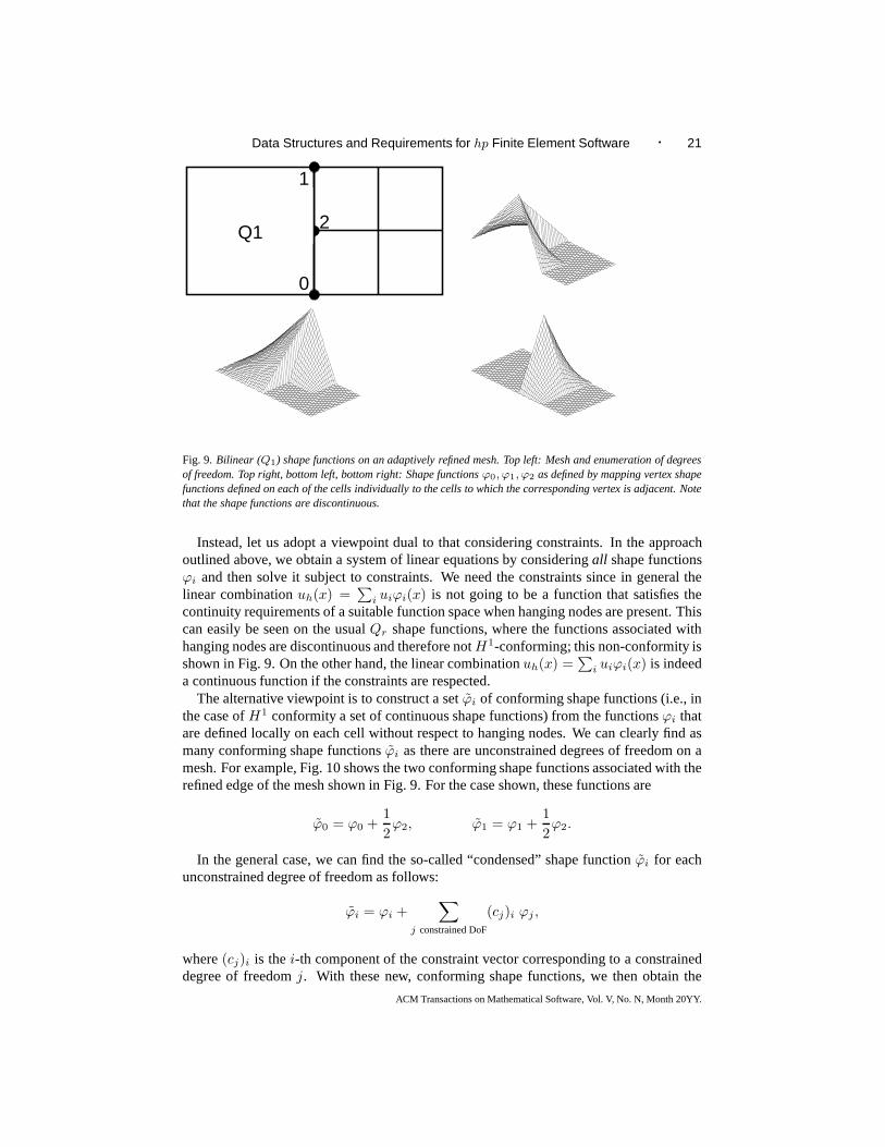
Fig. 9. Bilinear (Q1) shape functions on an adaptively refined mesh. Top left: Mesh and enumeration of degreesof freedom. Top right, bottom left, bottom right: Shape functionsϕ0, ϕ1, ϕ2 as defined by mapping vertex shapefunctions defined on each of the cells individually to the cells to which the corresponding vertex is adjacent. Notethat the shape functions are discontinuous.
Instead, let us adopt a viewpoint dual to that considering constraints. In the approachoutlined above, we obtain a system of linear equations by consideringall shape functionsϕi and then solve it subject to constraints. We need the constraints since in general thelinear combinationuh(x) =
∑
i uiϕi(x) is not going to be a function that satisfies thecontinuity requirements of a suitable function space when hanging nodes are present. Thiscan easily be seen on the usualQr shape functions, where the functions associated withhanging nodes are discontinuous and therefore notH1-conforming; this non-conformity isshown in Fig. 9. On the other hand, the linear combinationuh(x) =
∑
i uiϕi(x) is indeeda continuous function if the constraints are respected.
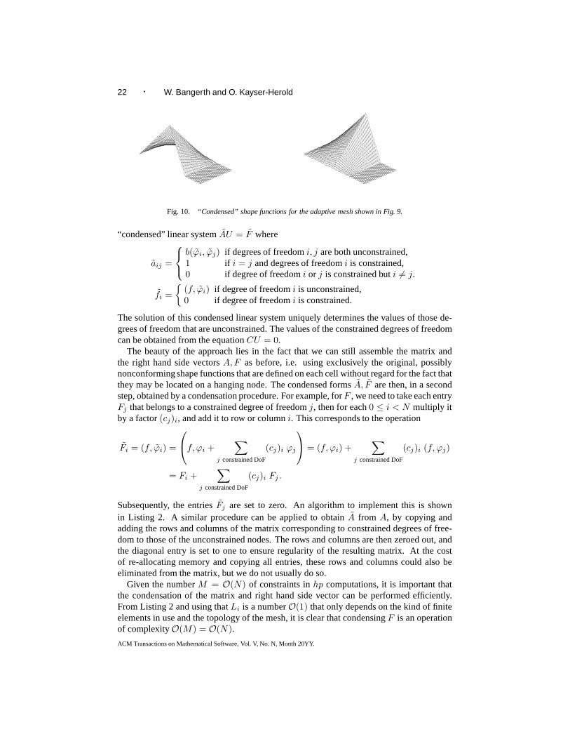
The alternative viewpoint is to construct a setϕi of conforming shape functions (i.e., inthe case ofH1 conformity a set of continuous shape functions) from the functionsϕi thatare defined locally on each cell without respect to hanging nodes. We can clearly find asmany conforming shape functionsϕi as there are unconstrained degrees of freedom on amesh. For example, Fig. 10 shows the two conforming shape functions associated with therefined edge of the mesh shown in Fig. 9. For the case shown, these functions are
ϕ0 = ϕ0 +1
2ϕ2, ϕ1 = ϕ1 +
1
2ϕ2.
In the general case, we can find the so-called “condensed” shape functionϕi for eachunconstrained degree of freedom as follows:
ϕi = ϕi +∑
j constrained DoF
(cj)i ϕj ,
where(cj)i is thei-th component of the constraint vector corresponding to a constraineddegree of freedomj. With these new, conforming shape functions, we then obtainthe
ACM Transactions on Mathematical Software, Vol. V, No. N, Month 20YY.
22 · W. Bangerth and O. Kayser-Herold
Fig. 10. “Condensed” shape functions for the adaptive mesh shown in Fig. 9.
“condensed” linear systemAU = F where
aij =
b(ϕi, ϕj) if degrees of freedomi, j are both unconstrained,1 if i = j and degrees of freedomi is constrained,0 if degree of freedomi or j is constrained buti 6= j.
fi =
(f, ϕi) if degree of freedomi is unconstrained,0 if degree of freedomi is constrained.
The solution of this condensed linear system uniquely determines the values of those de-grees of freedom that are unconstrained. The values of the constrained degrees of freedomcan be obtained from the equationCU = 0.
The beauty of the approach lies in the fact that we can still assemble the matrix andthe right hand side vectorsA,F as before, i.e. using exclusively the original, possiblynonconforming shape functions that are defined on each cell without regard for the fact thatthey may be located on a hanging node. The condensed formsA, F are then, in a secondstep, obtained by a condensation procedure. For example, forF , we need to take each entryFj that belongs to a constrained degree of freedomj, then for each0 ≤ i < N multiply itby a factor(cj)i, and add it to row or columni. This corresponds to the operation
Fi = (f, ϕi) =
f, ϕi +∑
j constrained DoF
(cj)i ϕj
= (f, ϕi) +∑
j constrained DoF
(cj)i (f, ϕj)
= Fi +∑
j constrained DoF
(cj)i Fj .
Subsequently, the entriesFj are set to zero. An algorithm to implement this is shownin Listing 2. A similar procedure can be applied to obtainA from A, by copying andadding the rows and columns of the matrix corresponding to constrained degrees of free-dom to those of the unconstrained nodes. The rows and columnsare then zeroed out, andthe diagonal entry is set to one to ensure regularity of the resulting matrix. At the costof re-allocating memory and copying all entries, these rowsand columns could also beeliminated from the matrix, but we do not usually do so.
Given the numberM = O(N) of constraints inhp computations, it is important thatthe condensation of the matrix and right hand side vector canbe performed efficiently.From Listing 2 and using thatLi is a numberO(1) that only depends on the kind of finiteelements in use and the topology of the mesh, it is clear that condensingF is an operationof complexityO(M) = O(N).
ACM Transactions on Mathematical Software, Vol. V, No. N, Month 20YY.
Data Structures and Requirements for hp Finite Element Software · 23
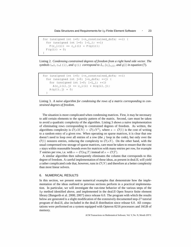
for (unsigned int i=0; i<n_constrained_dofs; ++i) for (unsigned int l=0; l<L_i; ++l)
F(r_l(i)) += c_i(l) * F(q(i));F(q(i)) = 0;
Listing 2. Condensing constrained degrees of freedom from a right handside vector. ThesymbolsL i, c i(l), andq(i) correspond toLi, (ci)rl(i), andq(i) in equation(7).
for (unsigned int i=0; i<n_constrained_dofs; ++i)for (unsigned int j=0; j<n_dofs; ++j)
for (unsigned int l=0; l<L_i; ++l)A(r_l(i),j) += c_i(l) * A(q(i),j);
A(q(i),j) = 0;
Listing 3. A naive algorithm for condensing the rows of a matrix corresponding to con-strained degrees of freedom.
The situation is more complicated when condensing matrices. First, it may be necessaryto add certain elements to the sparsity pattern of the matrix. Second, care must be takento avoid a quadratic complexity of the algorithm. Listing 3 shows a naive implementationof eliminating rows corresponding to constrained degrees of freedom. As written, thealgorithms complexity isO(sMN) = O(sN2), wheres = O(1) is the cost of writingto a random entry of a given row. When operating on sparse matrices, it is clear that onedoesn’t need to loop over all entries of a row (thej loop in the code), but only over theO(1) nonzero entries, reducing the complexity toO(sN). On the other hand, with theusual compressed row storage of sparse matrices, care must be taken to ensure that the costs stays within reasonable bounds even for matrices with many entries per row, for exampleT entries per row, i.e. withs = O(log T ) instead ofs = O(T ).
A similar algorithm then subsequently eliminates the column that corresponds to thisdegree of freedom. A careful implementation of these ideas,as present in deal.II, will yielda rather complicated code that, however, runs inO(N) and therefore at a better complexitythan most linear solvers.
6. NUMERICAL RESULTS
In this section, we present some numerical examples that demonstrate how the imple-mentation of the ideas outlined in previous sections perform in a practical implementa-tion. In particular, we will investigate the run-time behavior of the various steps of thehp method identified above, and implemented in the deal.II OpenSource finite elementlibrary [Bangerth et al. 2008; 2007] since release 6.0. The program with which the resultsbelow are generated is a slight modification of the extensively documented step-27 tutorialprogram of deal.II, also included in the deal.II distribution since release 6.0. All compu-tations were performed on a system equipped with Opteron 8216 processors and 16GB ofmemory.
ACM Transactions on Mathematical Software, Vol. V, No. N, Month 20YY.

24 · W. Bangerth and O. Kayser-Herold
no name no name
Fig. 11.Results for example 1. Left: The solutionu. Center: The mesh used for the discretization in the seventhadaptive refinement step. Right: The distribution of polynomial degrees onto cells.
Both numerical examples solve the linear Poisson equation,−∆u = f . Since all al-gorithms described above are independent of the actual problem solved, it is of no furtherconsequence that we do not solve a more complicated equation.
Example 1.In this first example, we solve on a square domain with a hole,Ω =[−1, 1]2\[− 1
2 ,12 ]2, using the right hand sidef(x, y) = (x + 1)(y + 1), and usinghp
finite elementsQk with orders2 ≤ k ≤ 8.The solution of this problem is shown in Fig. 11, together with the mesh after a few steps
of adaptive refinement and a distribution of finite elements onto this mesh.4 The algorithmto determine whether to refineh or increasep on a given cell uses an error indicator anda simple criterion to estimate the smoothness of the solution of this cell. Looking at theright panel of Fig. 11, we see that the polynomial degree is indeed low in the vicinity ofthe singularities close to re-entrant corners as well as along the boundary, and high in theinterior. This corresponds to the expected smoothness properties of the solution. Whetherthis particular arrangement of elements is in fact optimal (which it certainly isn’t) is outsidethe scope of this contribution: we only want to investigate how our algorithms perform for agiven distribution of finite elements onto a mesh, not the optimal choice of finite elements.For details of theh refinement andp assignment algorithms, we refer to the documentationof the step-27 tutorial program [Bangerth et al. 2008].
Given this, the left panel of Fig. 12 shows the growth of the number of degrees offreedom ashp refinement iterations proceed, as well the number of constrained degreesof freedom. The latter number is roughly constant at about 20% of the total.
The right panel shows a view of where the compute time for the numerical solution ofthis problem is spent. The total time used on each mesh grows approximately likeO(N1.5),whereN is the total number of degrees of freedom; this rate can be expected for the SSORpreconditioned Conjugate Gradient solver we use in this computation. This total computetime is in fact entirely dominated by solving the linear system, which consumes more than95% of the compute time forN ≥ 105.
The rest of the time is spent on assembling the linear system (3% for N=105) and variousother tasks. Among thehp specific activities, both allocating degrees of freedom (see thediscussion in Sections 3 and 4.2) and computing constraints(see Sections 4.3–4.5 and 5.1)take negligible fractions of the total compute time, and only the elimination of constrainednodes from the linear system (see Section 5.2) is noticeable. However, even the latter
4The solution looks blocky since we output it as a bilinear interpolation even on cells with high polynomialdegree. The actual computed solution is much more accurate than depicted.
ACM Transactions on Mathematical Software, Vol. V, No. N, Month 20YY.
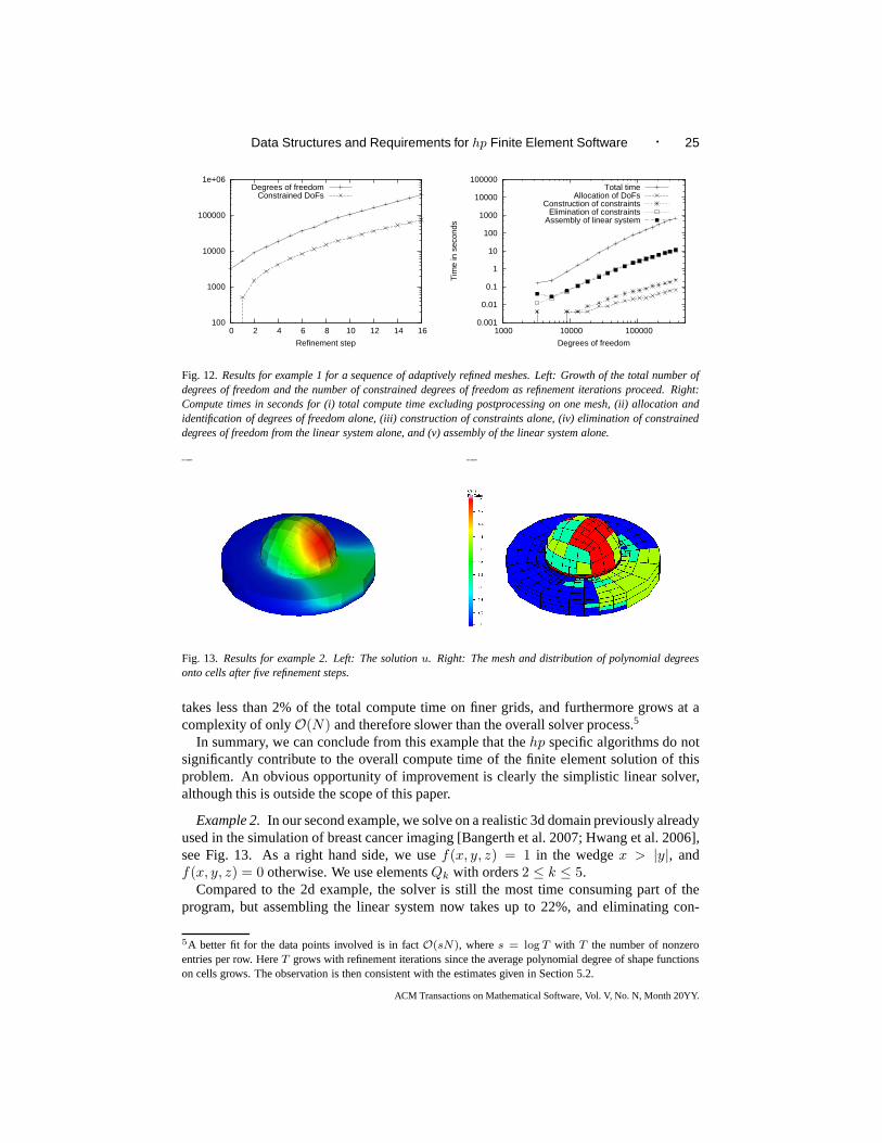
Data Structures and Requirements for hp Finite Element Software · 25
100
1000
10000
100000
1e+06
0 2 4 6 8 10 12 14 16
Refinement step
Degrees of freedomConstrained DoFs
0.001
0.01
0.1
1
10
100
1000
10000
100000
1000 10000 100000
Tim
e in
sec
onds
Degrees of freedom
Total timeAllocation of DoFs
Construction of constraintsElimination of constraints
Assembly of linear system
Fig. 12. Results for example 1 for a sequence of adaptively refined meshes. Left: Growth of the total number ofdegrees of freedom and the number of constrained degrees of freedom as refinement iterations proceed. Right:Compute times in seconds for (i) total compute time excluding postprocessing on one mesh, (ii) allocation andidentification of degrees of freedom alone, (iii) construction of constraints alone, (iv) elimination of constraineddegrees of freedom from the linear system alone, and (v) assembly of the linear system alone.
no name no name
Fig. 13. Results for example 2. Left: The solutionu. Right: The mesh and distribution of polynomial degreesonto cells after five refinement steps.
takes less than 2% of the total compute time on finer grids, andfurthermore grows at acomplexity of onlyO(N) and therefore slower than the overall solver process.5
In summary, we can conclude from this example that thehp specific algorithms do notsignificantly contribute to the overall compute time of the finite element solution of thisproblem. An obvious opportunity of improvement is clearly the simplistic linear solver,although this is outside the scope of this paper.
Example 2.In our second example, we solve on a realistic 3d domain previously alreadyused in the simulation of breast cancer imaging [Bangerth etal. 2007; Hwang et al. 2006],see Fig. 13. As a right hand side, we usef(x, y, z) = 1 in the wedgex > |y|, andf(x, y, z) = 0 otherwise. We use elementsQk with orders2 ≤ k ≤ 5.
Compared to the 2d example, the solver is still the most time consuming part of theprogram, but assembling the linear system now takes up to 22%, and eliminating con-
5A better fit for the data points involved is in factO(sN), wheres = log T with T the number of nonzeroentries per row. HereT grows with refinement iterations since the average polynomial degree of shape functionson cells grows. The observation is then consistent with the estimates given in Section 5.2.
ACM Transactions on Mathematical Software, Vol. V, No. N, Month 20YY.
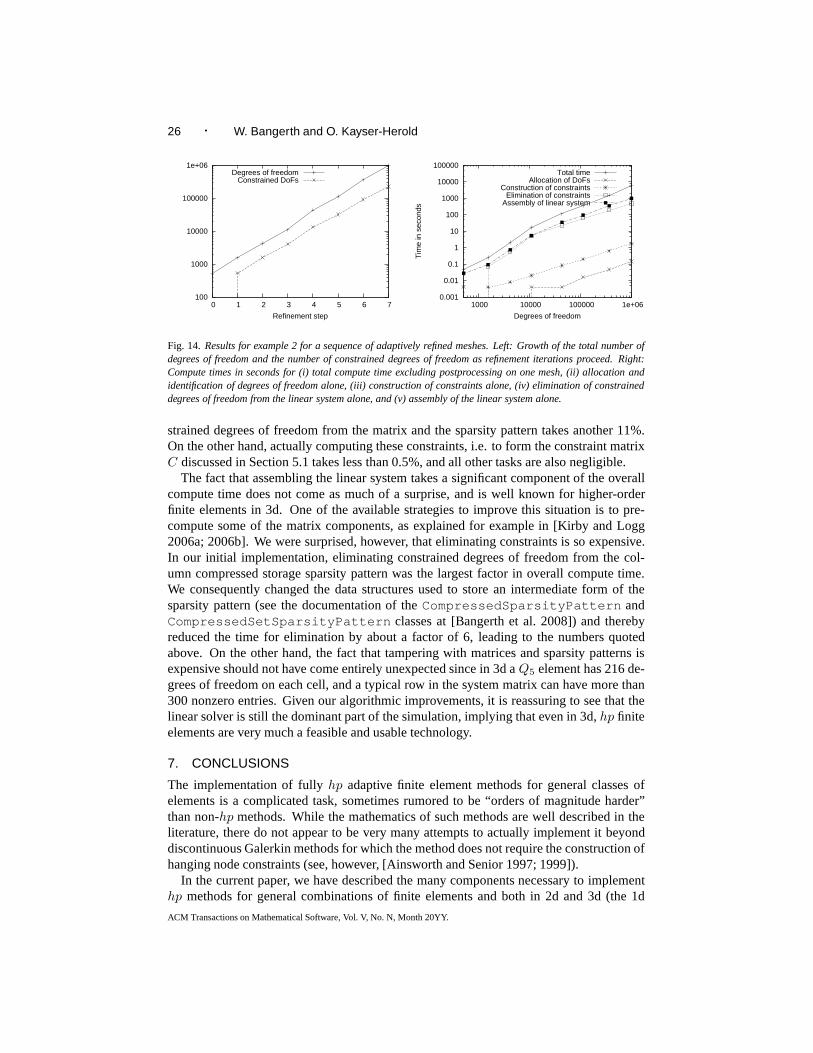
26 · W. Bangerth and O. Kayser-Herold
100
1000
10000
100000
1e+06
0 1 2 3 4 5 6 7
Refinement step
Degrees of freedomConstrained DoFs
0.001
0.01
0.1
1
10
100
1000
10000
100000
1000 10000 100000 1e+06
Tim
e in
sec
onds
Degrees of freedom
Total timeAllocation of DoFs
Construction of constraintsElimination of constraints
Assembly of linear system
Fig. 14. Results for example 2 for a sequence of adaptively refined meshes. Left: Growth of the total number ofdegrees of freedom and the number of constrained degrees of freedom as refinement iterations proceed. Right:Compute times in seconds for (i) total compute time excluding postprocessing on one mesh, (ii) allocation andidentification of degrees of freedom alone, (iii) construction of constraints alone, (iv) elimination of constraineddegrees of freedom from the linear system alone, and (v) assembly of the linear system alone.
strained degrees of freedom from the matrix and the sparsitypattern takes another 11%.On the other hand, actually computing these constraints, i.e. to form the constraint matrixC discussed in Section 5.1 takes less than 0.5%, and all other tasks are also negligible.
The fact that assembling the linear system takes a significant component of the overallcompute time does not come as much of a surprise, and is well known for higher-orderfinite elements in 3d. One of the available strategies to improve this situation is to pre-compute some of the matrix components, as explained for example in [Kirby and Logg2006a; 2006b]. We were surprised, however, that eliminating constraints is so expensive.In our initial implementation, eliminating constrained degrees of freedom from the col-umn compressed storage sparsity pattern was the largest factor in overall compute time.We consequently changed the data structures used to store anintermediate form of thesparsity pattern (see the documentation of theCompressedSparsityPattern andCompressedSetSparsityPattern classes at [Bangerth et al. 2008]) and therebyreduced the time for elimination by about a factor of 6, leading to the numbers quotedabove. On the other hand, the fact that tampering with matrices and sparsity patterns isexpensive should not have come entirely unexpected since in3d aQ5 element has 216 de-grees of freedom on each cell, and a typical row in the system matrix can have more than300 nonzero entries. Given our algorithmic improvements, it is reassuring to see that thelinear solver is still the dominant part of the simulation, implying that even in 3d,hp finiteelements are very much a feasible and usable technology.
7. CONCLUSIONS
The implementation of fullyhp adaptive finite element methods for general classes ofelements is a complicated task, sometimes rumored to be “orders of magnitude harder”than non-hp methods. While the mathematics of such methods are well described in theliterature, there do not appear to be very many attempts to actually implement it beyonddiscontinuous Galerkin methods for which the method does not require the construction ofhanging node constraints (see, however, [Ainsworth and Senior 1997; 1999]).
In the current paper, we have described the many components necessary to implementhp methods for general combinations of finite elements and bothin 2d and 3d (the 1d
ACM Transactions on Mathematical Software, Vol. V, No. N, Month 20YY.
Data Structures and Requirements for hp Finite Element Software · 27
case is so notably absent of any particular problems that we did not discuss our imple-mentation), and the complications and pitfalls one runs into. The techniques discussedhere provide the generic algorithms that can make this implementation work not only forQk elements, but general combinations of elements. Actual instances of finite elementclasses essentially only have to describe equivalences between degrees of freedom on ver-tices, edges, and faces, and provide matrices that describeinterpolation from one elementto another on faces and subfaces between cells. Beyond that,the generic algorithms dis-cussed can work independently of the actual elements involved. In particular, this includesH(div) [Brezzi and Fortin 1991] andH(curl) [Nedelec 1980] elements, but also immedi-ately vector-valued elements for problems with more than one solution variable.
In the final section of this paper, we also demonstrated that our algorithms are efficient,i.e. that they are cheap compared to the expensive parts of finite element programs: assem-bling linear systems and solving them. This demonstrates that it is possible to implementhp finite elements efficiently, even for continuous and 3d elements. A reference imple-mentation of our ideas, as well as the tutorial program step-27 explaining the use ofhpadaptivity, is available as part of the Open Source finite element library deal.II [Bangerthet al. 2008] since release 6.0.
Finally, we can also address the question whetherhp is hard to implement: we estimatethat to fully address the problems discussed in this paper, we had to implement less than20,000 lines of code on top of what deal.II already had to offer. This is comparable toprobably less than one year of work for a skilled and trained individual already familiarwith the internals of deal.II. This has to be compared to a total of roughly 360,000 lines ofcode presently in deal.II, of which maybe 100,000 are part ofthe low-level core that dealswith meshes, degrees of freedom, and finite elements. In other words, while a significantand certainly non-trivial task, the implementation of the ideas in this paper is clearly not“orders of magnitude” more difficult than a reasonably general implementation of the finiteelement method.
REFERENCES
A INSWORTH, M. AND SENIOR, B. 1997. Aspects of an adaptivehp-finite element method: Adaptive strategy,conforming approximation and efficient solvers.Comput. Methods Appl. Mech. Engrg. 150, 65–87.
A INSWORTH, M. AND SENIOR, B. 1999. hp-finite element procedures on non-uniform geometric meshes:Adaptivity and constrained approximation. InGrid Generation and Adaptive Algorithms, M. Bern, J. Flaherty,and M. Luskin, Eds. Number 113 in IMA Vol. Math. Appl. Springer, 1–27.
BABUSKA, I. 1981. Error estimates for the combinedh andp version of finite element method.Numer. Math. 37,252–277.
BANGERTH, W., HARTMANN , R.,AND KANSCHAT, G. 2007. deal.II – a general purpose object oriented finiteelement library.ACM Trans. Math. Softw. 33,4, 24/1–24/27.
BANGERTH, W., HARTMANN , R., AND KANSCHAT, G. 2008.deal.II Differential Equations Analysis Li-brary, Technical Reference. http://www.dealii.org/.
BREZZI, F. AND FORTIN, M. 1991.Mixed and Hybrid Finite Element Methods. Springer.
CAREY, G. F. 1997.Computational Grids: Generation, Adaptation and SolutionStrategies. Taylor & Francis.
CASTILLO , P., RIEBEN, R.,AND WHITE, D. 2005. FEMSTER: An object-oriented class library of higher-orderdiscrete differential forms.ACM Trans. Math. Software 31, 425–457.
CIARLET, P. G. 1978.The Finite Element Method for Elliptic Problems, First ed. Studies in Mathematics andits Applications, vol. 4. North-Holland, Amsterdam, New York, Oxford.
DEMKOWICZ, L. 2006. Computing with hp-adaptive finite elements. Volume 1: One and Two DimensionalElliptic and Maxwell Problems. Chapman & Hall.
ACM Transactions on Mathematical Software, Vol. V, No. N, Month 20YY.

28 · W. Bangerth and O. Kayser-Herold
FRAUENFELDER, P.AND LAGE, C. 2002. Concepts – An object-oriented software package for partial differen-tial equations.M2AN 36, 937–951.
GILBARG , D. AND TRUDINGER, N. S. 1983.Elliptic Partial Differential Equations of Second Order, Seconded. Springer, Heidelberg.
GUO, B. AND BABUSKA, I. 1986a. The h-p version of the finite element method. Part I: The basic approximationresults.Comp. Mech. 1, 21–41.
GUO, B. AND BABUSKA, I. 1986b. The h-p version of the finite element method. Part II: The general resultsand application.Comp. Mech. 1, 203–220.
HOUSTON, P., SCHOTZAU, D., AND WIHLER, T. P. 2007. Energy norm a posteriori error estimation ofhp-adaptive discontinuous galerkin methods for elliptic problems.M3AS 17, 33–62.
HOUSTON, P.AND SULI , E. 2005. A note on the design ofhp-adaptive finite element methods for elliptic partialdifferential equations.Comp. Meth. Appl. Mech. Engrg. 194, 229–243.
HOUSTON, P., SULI , E., AND WIHLER, T. P. 2008. A posteriori error analysis ofhp-version discontinuousGalerkin finite element methods for second-order quasilinear elliptic problems.IMA J. Numer. Anal., in press.
HWANG, K., PAN , T., JOSHI, A., RASMUSSEN, J. C., BANGERTH, W., AND SEVICK-MURACA, E. M. 2006.Influence of excitation light rejection on forward model mismatch in optical tomography.Phys. Med. Biol. 51,5889–5902.
K IRBY, R. AND LOGG, A. 2006a. A compiler for variational forms.ACM Trans. Math. Softw. 32, 417–444.K IRBY, R. AND LOGG, A. 2006b. Optimizing the FEniCS form compiler FFC: Efficient pretabulation of inte-
grals.submitted to ACM Trans. Math. Softw..K IRK , B., PETERSON, J. W., STOGNER, R. H., AND CAREY, G. F. 2006. libMesh: A C++ Library for
Parallel Adaptive Mesh Refinement/Coarsening Simulations. Engineering with Computers 22,3–4, 237–254.NEDELEC, J.-C. 1980. Mixed finite elements inR3. Numer. Math. 35, 315–341.PESCH, L., BELL , A., SOLLIE , H., AMBATI , V. R., BOKHOVE, O.,AND VAN DER VEGT, J. W. 2007. hpGEM –
A software framework for discontinuous Galerkin finite element methods.ACM Trans. Math. Softw. 33,4,23/1–23/25.
RHEINBOLDT, W. C. AND MESZTENYI, C. K. 1980. On a data structure for adaptive finite element meshrefinements.ACM Trans. Math. Software 6, 166–187.
RIVARA , M. C. 1984. Mesh refinement processes based on the generalized bisection of simplices.SIAM J.Numer. Anal. 21, 604–613.
SOLIN , P.,CERVENY , J.,AND DOLEZEL, I. 2008. Arbitrary-level hanging nodes and automatic adaptivity inthe hp-FEM.Math. Comput. Sim. 77, 117–132.
SOLIN , P., SEGETH, K., AND DOLEZEL, I. 2003. Higher-Order Finite Element Methods. Chapman & Hal-l/CRC.
ACM Transactions on Mathematical Software, Vol. V, No. N, Month 20YY.
Related Documents