DATA SCIENCE LABORATORY LAB MANUAL

DATA SCIENCE LABORATORY

LAB MANUAL

Course Code : BCSB10

Regulations : IARE - R18

Semester : I

Branch : CSE

Prepared By

Dr. R Obulakonda Reddy, Associate Professor

INSTITUTE OF AERONAUTICAL ENGINEERING (Autonomous)

Dundigal – 500 043, Hyderabad

INSTITUTE OF AERONAUTICAL ENGINEERING (Autonomous)

Dundigal – 500 043, Hyderabad

COMPUTER SCIENCE AND ENGINEERING

1. PROGRAM OUTCOMES:

M.TECH-PROGRAM OUTCOMES(POS)

PO1 Analyze a problem, identify and define computing requirements, design and implement

appropriate solutions

PO2 Solve complex heterogeneous data intensive analytical based problems of real time scenario

using state of the art hardware/software tools

PO3 Demonstrate a degree of mastery in emerging areas of CSE/IT like IoT, AI, Data Analytics,

Machine Learning, cyber security, etc.

PO4 Write and present a substantial technical report/document

PO5 Independently carry out research/investigation and development work to solve practical

problems

PO6 Function effectively on teams to establish goals, plan tasks, meet deadlines, manage risk and

produce deliverables

PO7 Engage in life-long learning and professional development through self-study, continuing

education, professional and doctoral level studies.

2. OBJECTIVES OF THE DEPARTMENT

DEPARTMENT OF COMPUTER SCIENCE AND ENGINEERING

Program Educational Objectives (PEOs)

A Post Graduate of the Computer Science and Engineering Program should:

PEO – I Independently design and develop computer software systems and products based on sound

theoretical principles and appropriate software development skills.

PEO–II Demonstrate knowledge of technological advances through active participation in life-long

learning.

PEO– III Accept to take up responsibilities upon employment in the areas of teaching, research,and

software development.

PEO– IV Exhibit technical communication, collaboration and mentoring skills and assume rolesboth

as team members and as team leaders in an organization.

3. ATTAINMENT OF PROGRAM OUTCOMES AND PROGRAM SPECIFIC OUTCOMES:

S. No

Experiment Program Outcomes

Attained

1

R AS CALCULATOR APPLICATION

a. Using with and without R objects on console

b. Using mathematical functions on console

c. Write an R script, to create R objects for

calculator application and save in a specified location

in disk.

PO1, PO5

2

DESCRIPTIVE STATISTICS IN R

a. Write an R script to find basic descriptive statistics using summary,

str, quartile function on mtcars& cars datasets.

b. Write an R script to find subset of dataset by using

subset (), aggregate () functions on iris dataset.

PO2, PO5

3

READING AND WRITING DIFFERENT TYPES OF DATASETS

a. Reading different types of data sets (.txt, .csv) from

Web and disk and writing in file in specific disk location.

b. Reading Excel data sheet in R.

c. Reading XML dataset in R.

PO1, PO6

4

VISUALIZATIONS

a. Find the data distributions using box and scatter plot.

b. Find the outliers using plot.

c. Plot the histogram, bar chart and pie chart on sample

data.

PO1, PO6

5

CORRELATION AND COVARIANCE

a. Find the correlation matrix.

b. Plot the correlation plot on dataset and visualize giving an overview of

relationships

among data on iris data.

c. Analysis of covariance: variance (ANOVA), if data have categorical

variables on iris data.

PO3, PO7

6

REGRESSION MODEL

Import a data from web storage. Name the dataset and now do Logistic

Regression to find out relation between variables that are affecting the

admission of a student in a institute based on his or her GRE score,

GPA obtained and rank of the student. Also check the model is fit or

not. Require (foreign), require (MASS).

PO6

7 MULTIPLE REGRESSION MODEL

Apply multiple regressions, if data have a continuous

Independent variable. Apply on above dataset.

PO5

8 REGRESSION MODEL FOR PREDICTION

Apply regression Model techniques to predict the data on

above dataset.

PO6, PO7

9

CLASSIFICATION MODEL

a. Install relevant package for classification.

b. Choose classifier for classification problem.

c. Evaluate the performance of classifier.

PO4, PO5

10 CLUSTERING MODEL

a. Clustering algorithms for unsupervised classification.

b. Plot the cluster data using R visualizations.

PO4, PO5

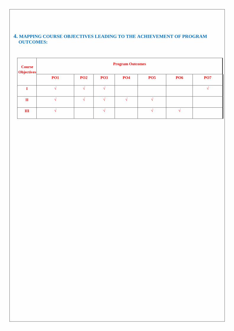
http://personality-project.org/r/r.205.tutorial.html#correlation

http://personality-project.org/r/r.205.tutorial.html#anova

4. MAPPING COURSE OBJECTIVES LEADING TO THE ACHIEVEMENT OF PROGRAM

OUTCOMES:

Course

Objectives

Program Outcomes

PO1 PO2 PO3 PO4 PO5 PO6 PO7

I √ √ √ √

II √ √ √ √ √

III √ √ √ √

5. SYLLABUS:

DATA SCIENCE LABORATORY

I Semester: CSE

Course Code Category Hours / Week Credits Maximum Marks

BCSB10 Core L T P C CIA SEE Total

- - 3 2 30 70 100

Contact Classes: Nil Total Tutorials: Nil Total Practical Classes: 36 Total Classes: 36

OBJECTIVES:

The course should enable the students to:

I. Understand the R Programming Language.

II. Exposure on Solving of data science problems.

III. Understand The classification and Regression Model.

LIST OF EXPERIMENTS

Week-1 R AS CALCULATOR APPLICATION



c. Write an R script, to create R objects for calculator application and save in a specified location in disk

Week-2 DESCRIPTIVE STATISTICS IN R

a. Write an R script to find basic descriptive statistics using summary

b. Write an R script to find subset of dataset by using subset ()

Week-3 READING AND WRITING DIFFERENT TYPES OF DATASETS

a. Reading different types of data sets (.txt, .csv) from web and disk and writing in file in specific disk

location.



Week-4 VISUALIZATIONS



c. Plot the histogram, bar chart and pie chart on sample data

Week-5 CORRELATION AND COVARIANCE

a. Find the correlation matrix.

b. Plot the correlation plot on dataset and visualize giving an overview of relationships among data on

iris data.


c. Analysis of covariance: variance (ANOVA), if data have categorical variables on iris data

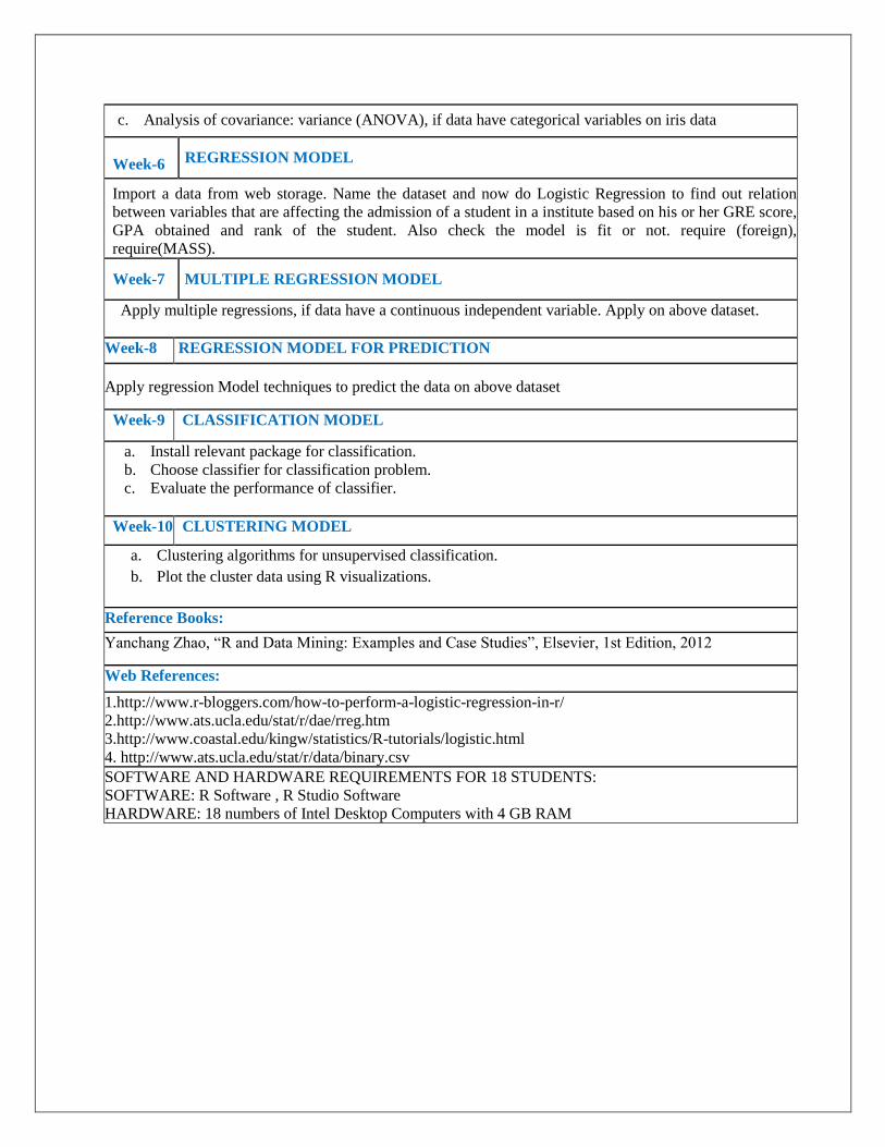
Week-6 REGRESSION MODEL

Import a data from web storage. Name the dataset and now do Logistic Regression to find out relation

between variables that are affecting the admission of a student in a institute based on his or her GRE score,

GPA obtained and rank of the student. Also check the model is fit or not. require (foreign),

require(MASS).

Week-7 MULTIPLE REGRESSION MODEL

Apply multiple regressions, if data have a continuous independent variable. Apply on above dataset.

Week-8 REGRESSION MODEL FOR PREDICTION

Apply regression Model techniques to predict the data on above dataset

Week-9 CLASSIFICATION MODEL

a. Install relevant package for classification.

b. Choose classifier for classification problem.

c. Evaluate the performance of classifier.

Week-10 CLUSTERING MODEL

a. Clustering algorithms for unsupervised classification.

b. Plot the cluster data using R visualizations.

Reference Books:

Yanchang Zhao, “R and Data Mining: Examples and Case Studies”, Elsevier, 1st Edition, 2012

Web References:

1.http://www.r-bloggers.com/how-to-perform-a-logistic-regression-in-r/

2.http://www.ats.ucla.edu/stat/r/dae/rreg.htm

3.http://www.coastal.edu/kingw/statistics/R-tutorials/logistic.html

4. http://www.ats.ucla.edu/stat/r/data/binary.csv

SOFTWARE AND HARDWARE REQUIREMENTS FOR 18 STUDENTS:

SOFTWARE: R Software , R Studio Software

HARDWARE: 18 numbers of Intel Desktop Computers with 4 GB RAM


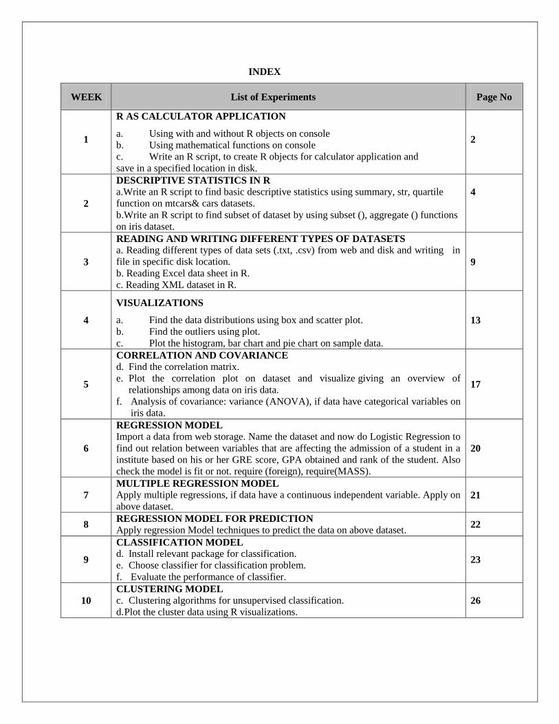
INDEX

WEEK List of Experiments Page No

1

R AS CALCULATOR APPLICATION



c. Write an R script, to create R objects for calculator application and

save in a specified location in disk.

2

2

DESCRIPTIVE STATISTICS IN R

a.Write an R script to find basic descriptive statistics using summary, str, quartile

function on mtcars& cars datasets.

b.Write an R script to find subset of dataset by using subset (), aggregate () functions

on iris dataset.

4

3

READING AND WRITING DIFFERENT TYPES OF DATASETS

a. Reading different types of data sets (.txt, .csv) from web and disk and writing in

file in specific disk location.



9

4

VISUALIZATIONS



c. Plot the histogram, bar chart and pie chart on sample data.

13

5

CORRELATION AND COVARIANCE

d. Find the correlation matrix.

e. Plot the correlation plot on dataset and visualize giving an overview of

relationships among data on iris data.

f. Analysis of covariance: variance (ANOVA), if data have categorical variables on

iris data.

17

6

REGRESSION MODEL

Import a data from web storage. Name the dataset and now do Logistic Regression to

find out relation between variables that are affecting the admission of a student in a

institute based on his or her GRE score, GPA obtained and rank of the student. Also

check the model is fit or not. require (foreign), require(MASS).

20

7

MULTIPLE REGRESSION MODEL

Apply multiple regressions, if data have a continuous independent variable. Apply on

above dataset. 21

8 REGRESSION MODEL FOR PREDICTION

Apply regression Model techniques to predict the data on above dataset. 22

9

CLASSIFICATION MODEL

d. Install relevant package for classification.

e. Choose classifier for classification problem.

f. Evaluate the performance of classifier.

23

10

CLUSTERING MODEL

c. Clustering algorithms for unsupervised classification.

d. Plot the cluster data using R visualizations. 26



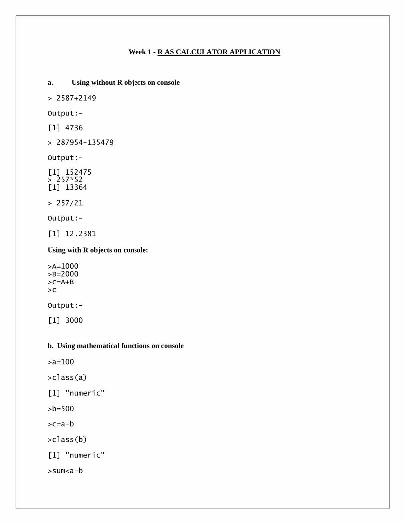
Week 1 - R AS CALCULATOR APPLICATION

a. Using without R objects on console

> 2587+2149 Output:- [1] 4736 > 287954-135479 Output:- [1] 152475 > 257*52 [1] 13364 > 257/21 Output:- [1] 12.2381 Using with R objects on console:

>A=1000 >B=2000 >c=A+B >c Output:- [1] 3000


>a=100 >class(a) [1] "numeric" >b=500 >c=a-b >class(b) [1] "numeric" >sum<a-b

[1] FALSE >sum [1] -400

c. Write an R script, to create R objects for calculator application andsave in a specified location in

disk.

getwd() [1] "C:/Users/Administrator/Documents" >write.csv(a,'a.csv') >write.csv(a,'C:\\Users\\Administrator\\Documents')

Week 2 - DESCRIPTIVE STATISTICS IN R

a. Write an R script to find basic descriptive statistics using summary, str, quartile function on mtcars&

cars datasets.

>mtcars mpgcyldisphp drat wtqsec vs am gear carb Mazda RX4 21.0 6 160.0 110 3.90 2.620 16.46 0 1 4 4 Mazda RX4 Wag 21.0 6 160.0 110 3.90 2.875 17.02 0 1 4 4 Datsun 710 22.8 4 108.0 93 3.85 2.320 18.61 1 1 4 1 Hornet 4 Drive 21.4 6 258.0 110 3.08 3.215 19.44 1 0 3 1 Hornet Sportabout 18.7 8 360.0 175 3.15 3.440 17.02 0 0 3 2 Valiant 18.1 6 225.0 105 2.76 3.460 20.22 1 0 3 1 Duster 360 14.3 8 360.0 245 3.21 3.570 15.84 0 0 3 4 Merc 240D 24.4 4 146.7 62 3.69 3.190 20.00 1 0 4 2 Merc 230 22.8 4 140.8 95 3.92 3.150 22.90 1 0 4 2 Merc 280 19.2 6 167.6 123 3.92 3.440 18.30 1 0 4 4 Merc 280C 17.8 6 167.6 123 3.92 3.440 18.90 1 0 4 4 Merc 450SE 16.4 8 275.8 180 3.07 4.070 17.40 0 0 3 3 Merc 450SL 17.3 8 275.8 180 3.07 3.730 17.60 0 0 3 3 Merc 450SLC 15.2 8 275.8 180 3.07 3.780 18.00 0 0 3 3 Cadillac Fleetwood 10.4 8 472.0 205 2.93 5.250 17.98 0 0 3 4 Lincoln Continental 10.4 8 460.0 215 3.00 5.424 17.82 0 0 3 4 Chrysler Imperial 14.7 8 440.0 230 3.23 5.345 17.42 0 0 3 4 Fiat 128 32.4 4 78.7 66 4.08 2.200 19.47 1 1 4 1 Honda Civic 30.4 4 75.7 52 4.93 1.615 18.52 1 1 4 2 Toyota Corolla 33.9 4 71.1 65 4.22 1.835 19.90 1 1 4 1 Toyota Corona 21.5 4 120.1 97 3.70 2.465 20.01 1 0 3 1 Dodge Challenger 15.5 8 318.0 150 2.76 3.520 16.87 0 0 3 2 AMC Javelin 15.2 8 304.0 150 3.15 3.435 17.30 0 0 3

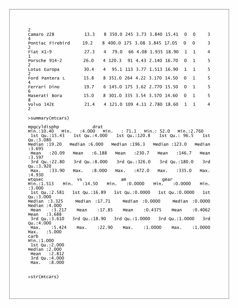
2 Camaro Z28 13.3 8 350.0 245 3.73 3.840 15.41 0 0 3 4 Pontiac Firebird 19.2 8 400.0 175 3.08 3.845 17.05 0 0 3 2 Fiat X1-9 27.3 4 79.0 66 4.08 1.935 18.90 1 1 4 1 Porsche 914-2 26.0 4 120.3 91 4.43 2.140 16.70 0 1 5 2 Lotus Europa 30.4 4 95.1 113 3.77 1.513 16.90 1 1 5 2 Ford Pantera L 15.8 8 351.0 264 4.22 3.170 14.50 0 1 5 4 Ferrari Dino 19.7 6 145.0 175 3.62 2.770 15.50 0 1 5 6 Maserati Bora 15.0 8 301.0 335 3.54 3.570 14.60 0 1 5 8 Volvo 142E 21.4 4 121.0 109 4.11 2.780 18.60 1 1 4 2 >summary(mtcars) mpgcyldisphp drat Min.:10.40 Min. :4.000 Min. : 71.1 Min.: 52.0 Min.:2.760 1st Qu.:15.43 1st Qu.:4.000 1st Qu.:120.8 1st Qu.: 96.5 1st Qu.:3.080 Median :19.20 Median :6.000 Median :196.3 Median :123.0 Median :3.695 Mean :20.09 Mean :6.188 Mean :230.7 Mean :146.7 Mean :3.597 3rd Qu.:22.80 3rd Qu.:8.000 3rd Qu.:326.0 3rd Qu.:180.0 3rd Qu.:3.920 Max. :33.90 Max. :8.000 Max. :472.0 Max. :335.0 Max. :4.930 wtqsec vs am gear Min.:1.513 Min. :14.50 Min. :0.0000 Min. :0.0000 Min. :3.000 1st Qu.:2.581 1st Qu.:16.89 1st Qu.:0.0000 1st Qu.:0.0000 1st Qu.:3.000 Median :3.325 Median :17.71 Median :0.0000 Median :0.0000 Median :4.000 Mean :3.217 Mean :17.85 Mean :0.4375 Mean :0.4062 Mean :3.688 3rd Qu.:3.610 3rd Qu.:18.90 3rd Qu.:1.0000 3rd Qu.:1.0000 3rd Qu.:4.000 Max. :5.424 Max. :22.90 Max. :1.0000 Max. :1.0000 Max. :5.000 carb Min.:1.000 1st Qu.:2.000 Median :2.000 Mean :2.812 3rd Qu.:4.000 Max. :8.000

>str(mtcars)

'data.frame': 32 obs. of 11 variables: $ mpg :num 21 21 22.8 21.4 18.7 18.1 14.3 24.4 22.8 19.2 ... $ cyl :num 6 6 4 6 8 6 8 4 4 6 ... $ disp: num 160 160 108 258 360 ... $ hp :num 110 110 93 110 175 105 245 62 95 123 ... $ drat: num 3.9 3.9 3.85 3.08 3.15 2.76 3.21 3.69 3.92 3.92 ... $ wt :num 2.62 2.88 2.32 3.21 3.44 ... $ qsec: num 16.5 17 18.6 19.4 17 ... $ vs :num 0 0 1 1 0 1 0 1 1 1 ... $ am :num 1 1 1 0 0 0 0 0 0 0 ... $ gear: num 4 4 4 3 3 3 3 4 4 4 ... $ carb: num 4 4 1 1 2 1 4 2 2 4 ... >quantile(mtcars$mpg) 0% 25% 50% 75% 100% 10.400 15.425 19.200 22.800 33.900 >cars speeddist 1 4 2 2 4 10 3 7 4 4 7 22 5 8 16 6 9 10 7 10 18 8 10 26 9 10 34 10 11 17 11 11 28 12 12 14 13 12 20 14 12 24 15 12 28 16 13 26 17 13 34 18 13 34 19 13 46 20 14 26 21 14 36 22 14 60 23 14 80 24 15 20 25 15 26 26 15 54 27 16 32 28 16 40 29 17 32 30 17 40 31 17 50 32 18 42 33 18 56 34 18 76 35 18 84 36 19 36

37 19 46 38 19 68 39 20 32 40 20 48 41 20 52 42 20 56 43 20 64 44 22 66 45 23 54 46 24 70 47 24 92 48 24 93 49 24 120 50 25 85 >summary(cars) speeddist Min.: 4.0 Min. : 2.00 1st Qu.:12.0 1st Qu.: 26.00 Median :15.0 Median : 36.00 Mean :15.4 Mean : 42.98 3rd Qu.:19.0 3rd Qu.: 56.00 Max. :25.0 Max. :120.00 >class(cars) [1] "data.frame" >dim(cars) [1] 50 2 >str(cars) 'data.frame': 50 obs. of 2 variables: $ speed: num 4 4 7 7 8 9 10 10 10 11 ... $ dist :num 2 10 4 22 16 10 18 26 34 17 ... >quantile(cars$speed) 0% 25% 50% 75% 100% 4 12 15 19 25

b. Write an R script to find subset of dataset by using subset (), aggregate () functions on iris dataset. >aggregate(. ~ Species, data = iris, mean)

Output:

Species Sepal.LengthSepal.WidthPetal.LengthPetal.Width

1 setosa 5.006 3.428 1.462 0.246

2 versicolor 5.936 2.770 4.260 1.326

3 virginica 6.588 2.974 5.552 2.026

>subset(iris,iris$Sepal.Length==5.0)

Output: Sepal.LengthSepal.WidthPetal.LengthPetal.WidthSpecies

5 5 3.6 1.4 0.2 setosa

8 5 3.4 1.5 0.2 setosa

26 5 3.0 1.6 0.2 setosa

27 5 3.4 1.6 0.4 setosa

36 5 3.2 1.2 0.2 setosa

41 5 3.5 1.3 0.3 setosa

44 5 3.5 1.6 0.6 setosa

50 5 3.3 1.4 0.2 setosa

61 5 2.0 3.5 1.0 versicolor

94 5 2.3 3.3 1.0 versicolor

Week 3 - READING AND WRITING DIFFERENT TYPES OF DATASETS

a. Reading different types of data sets (.txt, .csv) from web and disk and writing in file in specific disk

location.

library(utils)

data<- read.csv("input.csv")

data

Output :-

id, name, salary, start_date, dept

1 1 Rick 623.30 2012-01-01 IT

2 2 Dan 515.20 2013-09-23 Operations

3 3 Michelle 611.00 2014-11-15 IT

4 4 Ryan 729.00 2014-05-11 HR

5 NA Gary 843.25 2015-03-27 Finance

6 6 Nina 578.00 2013-05-21 IT

7 7 Simon 632.80 2013-07-30 Operations

8 8 Guru 722.50 2014-06-17 Finance


print(is.data.frame(data))

print(ncol(data))

print(nrow(data))

Output:-

[1] TRUE

[1] 5

[1] 8

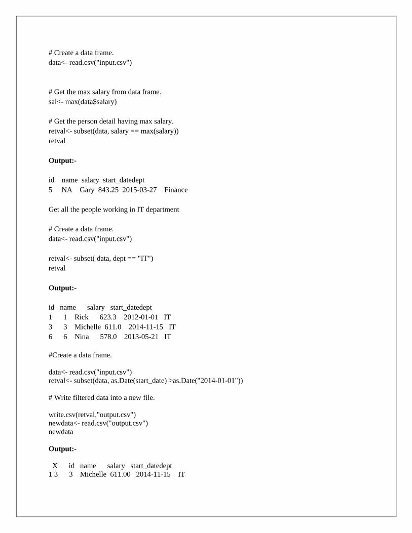
# Create a data frame.


# Get the max salary from data frame.

sal<- max(data$salary)

sal

Output:-

[1] 843.25



# Get the max salary from data frame.

sal<- max(data$salary)

# Get the person detail having max salary.

retval<- subset(data, salary == max(salary))

retval

Output:-

id name salary start_datedept

5 NA Gary 843.25 2015-03-27 Finance

Get all the people working in IT department



retval<- subset( data, dept == "IT")

retval

Output:-

id name salary start_datedept

1 1 Rick 623.3 2012-01-01 IT

3 3 Michelle 611.0 2014-11-15 IT

6 6 Nina 578.0 2013-05-21 IT

#Create a data frame.


retval<- subset(data, as.Date(start_date) >as.Date("2014-01-01"))

# Write filtered data into a new file.

write.csv(retval,"output.csv")

newdata<- read.csv("output.csv")

newdata

Output:-

X id name salary start_datedept

1 3 3 Michelle 611.00 2014-11-15 IT

2 4 4 Ryan 729.00 2014-05-11 HR

3 5 NA Gary 843.25 2015-03-27 Finance

4 8 8 Guru 722.50 2014-06-17 Finance


install.packages("xlsx")

library("xlsx")

data<- read.xlsx("input.xlsx", sheetIndex = 1)

data

Output:-

id, name, salary, start_date, dept

1 1 Rick 623.30 2012-01-01 IT

2 2 Dan 515.20 2013-09-23 Operations

3 3 Michelle 611.00 2014-11-15 IT

4 4 Ryan 729.00 2014-05-11 HR

5 NA Gary 843.25 2015-03-27 Finance

6 6 Nina 578.00 2013-05-21 IT

7 7 Simon 632.80 2013-07-30 Operations

8 8 Guru 722.50 2014-06-17 Finance

c. Reading XML dataset in R. install.packages("XML") library("XML") library("methods") result<- xmlParse(file = "input.xml") result Output:- 1 Rick 623.3 1/1/2012 IT 2 Dan 515.2 9/23/2013

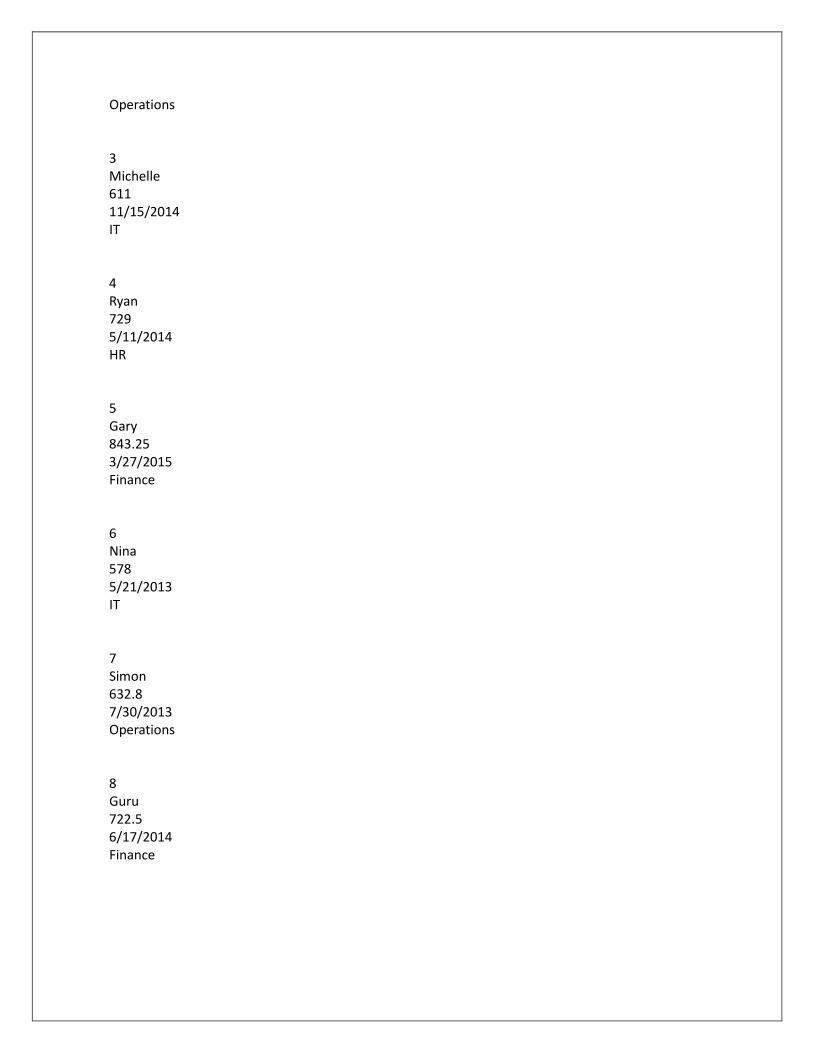
Operations 3 Michelle 611 11/15/2014 IT 4 Ryan 729 5/11/2014 HR 5 Gary 843.25 3/27/2015 Finance 6 Nina 578 5/21/2013 IT 7 Simon 632.8 7/30/2013 Operations 8 Guru 722.5 6/17/2014 Finance

Week 4 – VISUALIZATIONS


Install.packages(“ggplot2”)

Library(ggplot2)

Input <- mtcars[,c('mpg','cyl')]

input

Boxplot(mpg ~ cyl, data = mtcars, xlab = "number of cylinders",

ylab = "miles per gallon", main = "mileage data")

Dev.off()

Output :-

mpg cyl

Mazda rx4 21.0 6

Mazda rx4 wag 21.0 6

Datsun 710 22.8 4

Hornet 4 drive 21.4 6

Hornet sportabout 18.7 8

Valiant 18.1 6


v=c(50,75,100,125,150,175,200)

boxplot(v)

c. Plot the histogram, bar chart and pie chart on sample data.

Histogram

library(graphics)

v <- c(9,13,21,8,36,22,12,41,31,33,19)

# Create the histogram.

hist(v,xlab = "Weight",col = "blue",border = "green")

dev.off()

Output:-

Bar chart

library(graphics)

H <- c(7,12,28,3,41)

M <- c("Jan","Feb","Mar","Apr","May")

# Plot the bar chart.

barplot(H,names.arg = M,xlab = "Month",ylab = "Revenue",col = "blue",main = "Revenue chart",border

= "red")

dev.off()

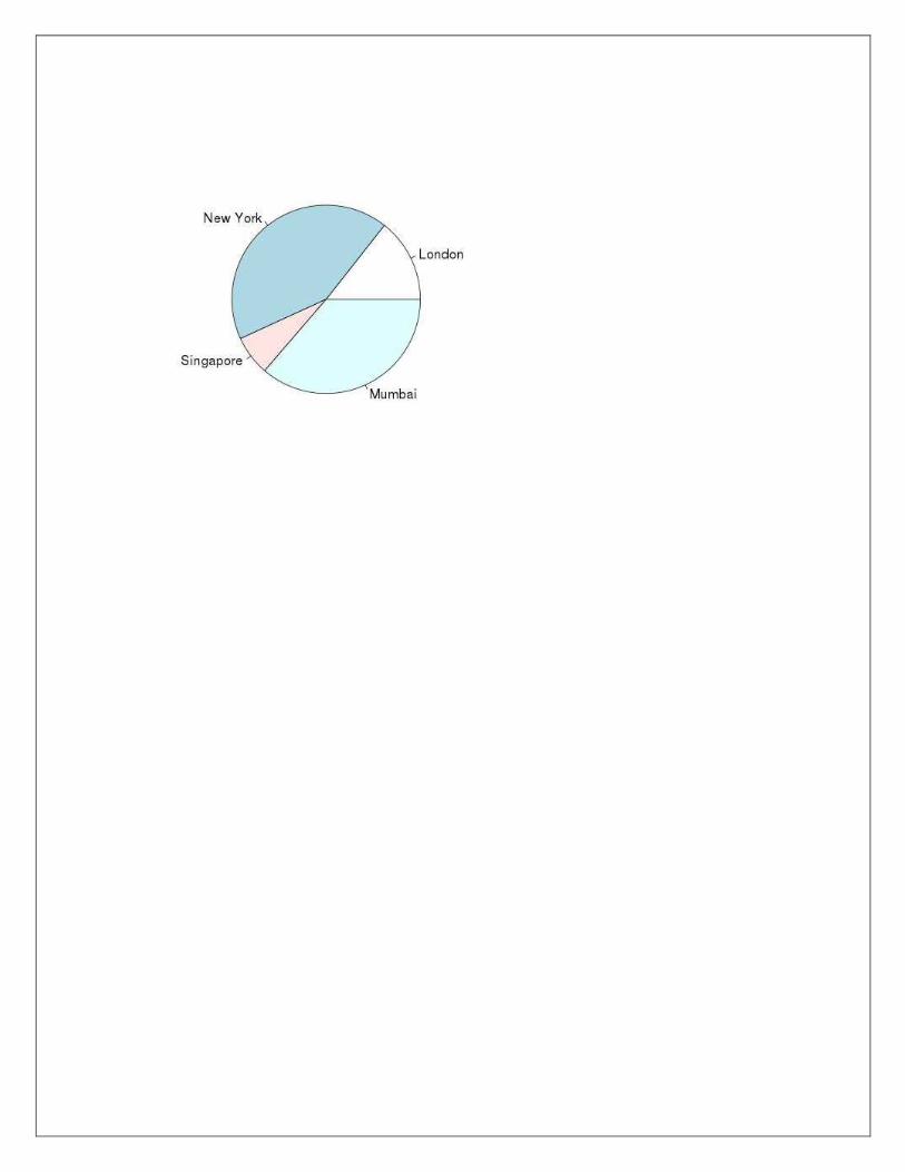
Pie Chart

library(graphics)

x <- c(21, 62, 10, 53)

labels<- c("London", "NewYork", "Singapore", "Mumbai")

# Plot the Pie chart.

pie(x,labels)

dev.off()

WEEK5:

PROBLEM DEFINATION:

a)How to find a corelation matrix and plot the correlation on iris data set SOURCE CODE: d<-data.frame(x1=rnorm(!0),x2=rnorm(10),x3=rnorm(10))

cor(d)

m<-cor(d) #get correlations

library(„corrplot‟)

corrplot(m,method=”square”)

x<-matrix(rnorm(2),,nrow=5,ncol=4)

y<-matrix(rnorm(15),nrow=5,ncol=3)

COR<-cor(x,y)

COR

PROBLEM DEFINATION:

b) Plot the correlation plot on dataset and visualize giving an overview of relationships among

data on iris data.

SOURCE CODE:

Image(x=seq(dim(x)[2])

Y<-seq(dim(y)[2])

Z=COR,xlab=”xcolumn”,ylab=”y column”)

Library(gtlcharts)

Data(iris)

Iris$species<-NULL

Iplotcorr(iris,reoder=TRUE

PROBLEM DEFINATION:

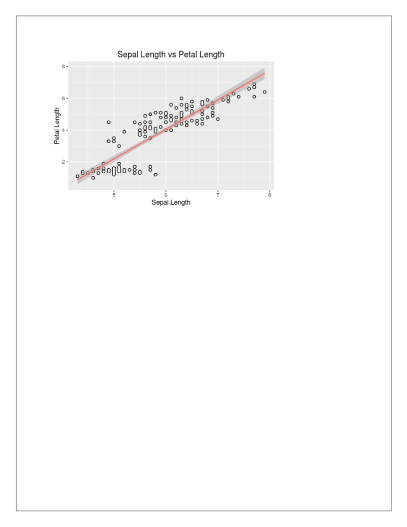
c) Analysis of covariance: variance (ANOVA), if data have categorical variables on iris data.

SOURCE CODE:

library(ggplot2)

data(iris)

str(iris)

ggplot(data=iris,aes(x=sepal.length,y=petal.length))+geom_point(size=2,colour=”black”)+geom_

point(size=1,colour=”white”)+geom_smooth(aes(colour=”black”),method=”lm‟)+ggtitle(“sepal.l

engthvspetal.length”)+xlab(“sepal.length”)+ylab(“petal.length”)+these(legend.position=”none”)


OUTPUT:

WEEK 6

PROBLEM DEFINATION: REGRESSION MODEL: Import a data from web storage. Name the dataset and now do Logistic

Regression to find out relation between variables that are affecting the admission of a student in a institute

based on his or her GRE score, GPA obtained and rank of the student. Also check the model is fit or not.

require (foreign), require(MASS)

SOURCE CODE:

mydata<-read.csv(http://www.ats.ucla.edu/stat/data/binary.csv”)

Head(my data)

OUTPUT:

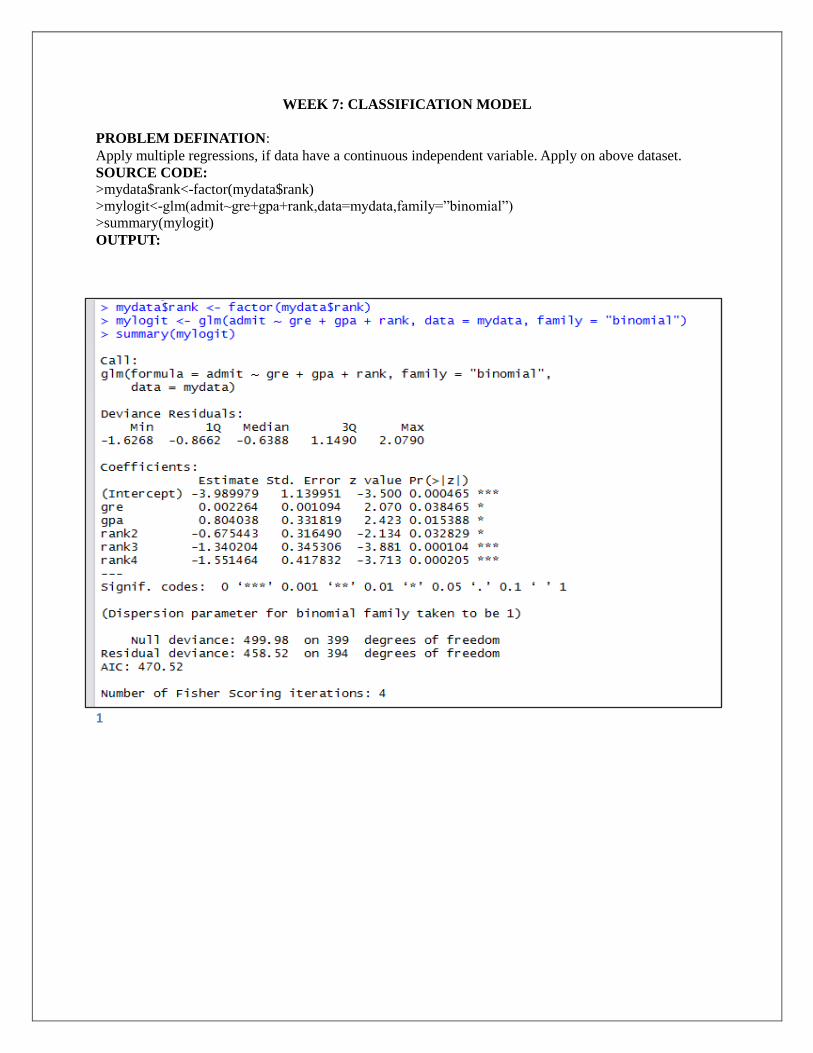
http://www.ats.ucla.edu/stat/data/binary.csv

WEEK 7: CLASSIFICATION MODEL

PROBLEM DEFINATION: Apply multiple regressions, if data have a continuous independent variable. Apply on above dataset.

SOURCE CODE:

>mydata$rank<-factor(mydata$rank)

>mylogit<-glm(admit~gre+gpa+rank,data=mydata,family=”binomial”)

>summary(mylogit)

OUTPUT:

1

Week 8 - REGRESSION MODEL FOR PREDICTION

Apply regression Model techniques to predict the data on above dataset.

># make sure R knows region is categorical

>str(states.data$region)

Factor w/ 4 levels "West","N. East",..: 3 1 1 3 1 1 2 3 NA 3 ...

>states.data$region<- factor(states.data$region)

> #Add region to the model

>sat.region<- lm(csat ~ region,

+ data=states.data)

> #Show the results

>coef(summary(sat.region)) # show regression coefficients table

Out put:

Estimate Std. Error t value Pr(>|t|)

(Intercept) 946.3 14.8 63.958 1.35e-46

regionN. East -56.8 23.1 -2.453 1.80e-02

regionSouth -16.3 19.9 -0.819 4.17e-01

regionMidwest 63.8 21.4 2.986 4.51e-03

>anova(sat.region) # show ANOVA table

Analysis of Variance Table

Response: csat

Df Sum Sq Mean Sq F value Pr(>F)

region 3 82049 27350 9.61 0.000049

Residuals 46 130912 2846

>

WEEK 9 :CLASSIFICATION MODEL

PROBLEM DEFINATION: g. Install relevant package for classification.

SOURCE CODE:

install.packages("rpart.plot")

install.packages("tree")

install.packages("ISLR")

install.packages("rattle")

library(tree)

library(ISLR)

library(rpart.plot)

library(rattle)

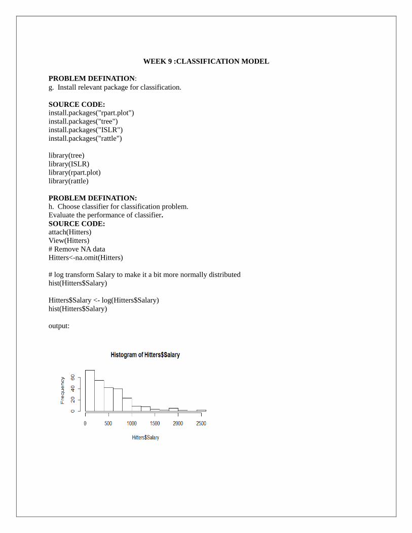
PROBLEM DEFINATION:

h. Choose classifier for classification problem.

Evaluate the performance of classifier.

SOURCE CODE:

attach(Hitters)

View(Hitters)

# Remove NA data

Hitters<-na.omit(Hitters)

# log transform Salary to make it a bit more normally distributed

hist(Hitters$Salary)

Hitters$Salary <- log(Hitters$Salary)

hist(Hitters$Salary)

output:

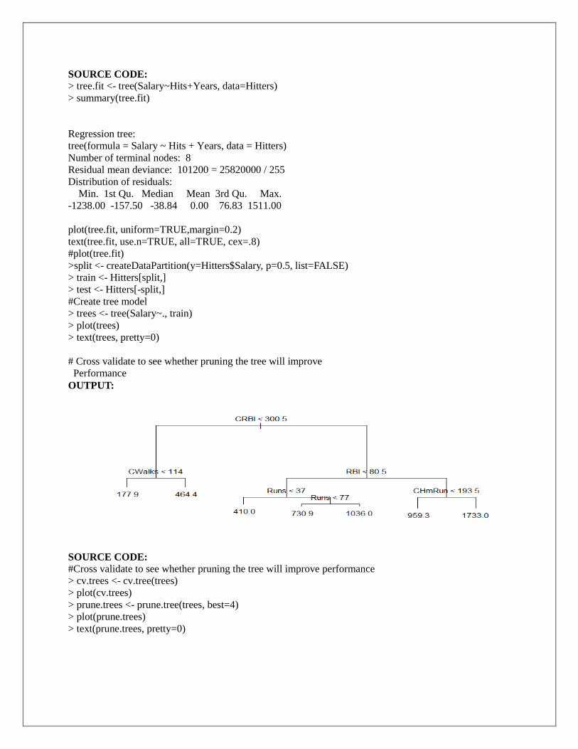
SOURCE CODE:

> tree.fit <- tree(Salary~Hits+Years, data=Hitters)

> summary(tree.fit)

Regression tree:

tree(formula = Salary ~ Hits + Years, data = Hitters)

Number of terminal nodes: 8

Residual mean deviance: 101200 = 25820000 / 255

Distribution of residuals:

Min. 1st Qu. Median Mean 3rd Qu. Max.

-1238.00 -157.50 -38.84 0.00 76.83 1511.00

plot(tree.fit, uniform=TRUE,margin=0.2)

text(tree.fit, use.n=TRUE, all=TRUE, cex=.8)

#plot(tree.fit)

>split <- createDataPartition(y=Hitters$Salary, p=0.5, list=FALSE)

> train <- Hitters[split,]

> test <- Hitters[-split,]

#Create tree model

> trees <- tree(Salary~., train)

> plot(trees)

> text(trees, pretty=0)

# Cross validate to see whether pruning the tree will improve

Performance

OUTPUT:

SOURCE CODE: #Cross validate to see whether pruning the tree will improve performance

> cv.trees <- cv.tree(trees)

> plot(cv.trees)

> prune.trees <- prune.tree(trees, best=4)

> plot(prune.trees)

> text(prune.trees, pretty=0)

OUTPUT:

SOURCE CODE:

> yhat <- predict(prune.trees, test)

> plot(yhat, test$Salary)

> abline(0,1

[1] 150179.7

> mean((yhat - test$Salary)^2)

[1] 150179.7

OUTPUT:

> mean((yhat - test$Salary)^2)

[1] 150179.7

WEEK 10

PROBLEM DEFINATION:

CLUSTERING MODEL

e. Clustering algorithms for unsupervised classification.

Plot the cluster data using R visualizations

SOURCE CODE:

1. Clustering algorithms for unsupervised classification.

library(cluster)

> set.seed(20)

> irisCluster <- kmeans(iris[, 3:4], 3, nstart = 20)

# nstart = 20. This means that R will try 20 different random starting assignments and then select the one

with the lowest within cluster variation.

> irisCluster

OUTPUT:

Petal.Length Petal.Width

1 1.462000 0.246000

2 4.269231 1.342308

3 5.595833 2.037500

Clustering vector:

[1] 1 1 1 1 1 1 1 1 1 1 1 1 1 1 1 1 1 1 1 1 1 1 1 1 1 1 1 1 1 1 1 1 1 1 1 1 1 1 1 1 1

[42] 1 1 1 1 1 1 1 1 1 2 2 2 2 2 2 2 2 2 2 2 2 2 2 2 2 2 2 2 2 2 2 2 2 2 2 2 3 2 2 2 2

[83] 2 3 2 2 2 2 2 2 2 2 2 2 2 2 2 2 2 2 3 3 3 3 3 3 2 3 3 3 3 3 3 3 3 3 3 3 3 2 3 3 3

[124] 3 3 3 2 3 3 3 3 3 3 3 3 3 3 3 2 3 3 3 3 3 3 3 3 3 3 3

Within cluster sum of squares by cluster:

[1] 2.02200 13.05769 16.29167

(between_SS / total_SS = 94.3 %)

Available components:

[1] "cluster" "centers" "totss" "withinss" "tot.withinss"

[6] "betweenss" "size" "iter" "ifault"

SOURCE CODE:

> irisCluster$cluster <- as.factor(irisCluster$cluster)

> ggplot(iris, aes(Petal.Length, Petal.Width, color = irisCluster$cluster)) + geom_point()

OUTPUT:

SOURCE CODE:

> d <- dist(as.matrix(mtcars)) # find distance matrix

> hc <- hclust(d) # apply hirarchical clustering

> plot(hc) # plot the dendrogram

OUTPUT:

2. Plot the cluster data using R visualizations.

SOURCE CODE:

## generate 25 objects, divided into 2 clusters.

x <- rbind(cbind(rnorm(10,0,0.5), rnorm(10,0,0.5)),

cbind(rnorm(15,5,0.5), rnorm(15,5,0.5)))

clusplot(pam(x, 2))

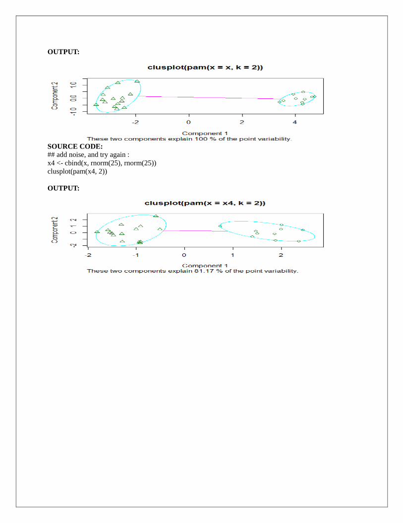
OUTPUT:

SOURCE CODE:

## add noise, and try again :

x4 <- cbind(x, rnorm(25), rnorm(25))

clusplot(pam(x4, 2))

OUTPUT: