Data reconciliation: a robust approach using a contaminated ...

Data reconciliation: a robust approach using a

contaminated distribution

Moustapha Alhaj-Dibo, Didier Maquin ∗ , Jose Ragot

Institut National Polytechnique de Lorraine

Centre de Recherche en Automatique de Nancy – UMR 7039 CNRS–UHP–INPL

2, Avenue de la foret de Haye, 54516 Vandœuvre-les-Nancy Cedex, FRANCE

Abstract

On-line optimisation provides a means for maintaining a process around its opti-mum operating range. This optimisation heavily relies on process measurementsand accurate process models. However, these measurements often contain randomand possibly gross errors as a result of miscalibration or failure of the measuringinstruments. This paper proposes a data reconciliation strategy that deals withthe presence of such gross errors. Instead of constructing the objective function tobe minimized on the basis of random errors only, the proposed method takes intoaccount both contributions from random and gross errors using a so-called contam-inated Gaussian distribution. It is shown that this approach introduces less bias inthe estimation due to its natural property to reject gross errors.

Key words: Data reconciliation, Robust estimation, Gross error detection, Linearand bilinear mass balances.

∗ Corresponding author. Tel.: +33 3 83 59 56 83; fax: + 33 3 83 59 56 44Email address: [email protected] (Didier Maquin).

Preprint submitted to Elsevier Science 28 November 2006

1 Introduction

The problem of obtaining reliable estimates of the state of a process is a fun-damental objective in process control and supervision, these estimates beingused to understand the process behaviour. For that purpose, a wide vari-ety of techniques has been developed to perform what is currently known asdata reconciliation (Mah, Stanley, Downing, 1976), (Maquin, Bloch, Ragot,1991). Data reconciliation, which is sometimes referred too as mass and en-ergy balance equilibration, is the adjustment of a set of data so the quanti-ties extracted from the data obey physical laws such as material and energyconservation. Since the pionner works devoted to the so-called data rectifica-tion (Himmelblau, 1978), the scope of research has expanded to cover otherfields such as data redundancy analysis, system observability, optimal sensorpositionning, sensor reliability, error characterization, measurement varianceestimation. Many applications are related in scientific papers involving variousfields in process engineering (Dhurjati, Cauvin, 1999), (Heyen, 1999), (Singh,Mittal, Sen, 2001), (Yi, Kim, Han, 2002).

Process measurements are inevitably corrupted by errors during the measure-ment itself but also during its processing and transmission stages. The totalerror in a measurement, which is the difference between the measured valueand the (definitely unknown) value of a variable, can be conveniently rep-resented as the sum of the contributions from two types of errors : randomand gross errors. Random errors which are inherent to the measurement pro-cess are usually small in magnitude and are most often described by the useof probability distributions. On the other hand, gross errors are caused bynon random events such as instrument malfunctioning, miscalibration, wearor corrosion of sensors and so on. The nonrandom nature of these errors im-plies that at any given time they have a certain magnitude and sign whichmay be unknown. Thus, if the measurement is repeated with the same instru-ment under identical conditions, the contribution of a systematic gross errorto the measurement value will be the same (Narasimhan, Jordache, 2000). Itis the reason why gross errors are also called systematic errors or biases. Inthe sequel of the paper all these terms will be employed without distinction.However, despite this strict definition of gross errors, a means for elaboratingrobust estimators of process variables consists to consider gross errors as ran-dom variables. For Veverka, Madron (1997), “Statistically, a gross error is anerror whose occurrence as realization of a random variable is highly unlikely”.This trick will be clearly justified in the section 3.2 dedicated to the use of acontaminated distribution.

As previously said the measurements collected on the process may be unknow-ingly corrupted by gross errors. As a result, the data reconciliation procedurecan give rise to absurd results and, in particular, the estimated variables are

2

most often corrupted by these biased data. Several schemes have been sug-gested to cope with the corruption of normal assumption of the errors, forstatic systems (Narasimhan, Mah, 1989), (Kim, Kang, Park, Edgar, 1997),(Arora, Biegler, 2001), (Soderstrom, Himmelblau, Edgar, 2001) and also fordynamic systems (Abu-el-zeet, Roberts, Becerra, 2001). Methods for includ-ing bounds in process variables to improve gross error detection have alsobeen developed. One major disadvantage of these methods is that they leadto situations where it may be impossible to estimate all the variable by usingonly a subset of the remaining gross errors free measurements. Alternativeapproach using constraints both on the estimates and the balance residualequations has been developed for linear system (Ragot, Maquin, Adrot, 1999),(Ragot, Maquin, 2004). Johnston, Kramer (1995) established an analogy be-tween maximum likelihood estimation and robust regression and they reportedthe feasibility and better performance of the robust estimators as the objec-tive function in the data reconciliation problem when the data contain grosserrors. These studies have been based on robust statistics and their ability toreject outliers (Huber, 1981), (Hampel, Ronchetti, Rousseeuw, Stohel, 1986).This kind of approach will be recalled in the first part of section 3. Anotherapproach is to take into account the non ideality of the measurement errordistribution by using an objective function constructed on contaminated errordistribution (Tjoa, Biegler, 1991), (Ozyurt, Pike, 2004). In the following, thisidea is adopted and developed for the data reconciliation problem.

The next section is devoted to recall the background of data reconciliationbased on the assumption that all the measurements are normally distributed.Robust data reconciliation method is described in section 3. In a first part,the main idea is introduced based on the use of the so-called generalizedmaximum likelihood function. The second part presents the proposed methodwhich make use of a contaminated error distribution. The previous results areestablished in the context of linear models, so the next section extends themethod to the bilinear case. Section 5 shows the adaptation of the method tothe frequently encountered case of partial measurements. Finally, the proposedmethod is implemented on a fictitious but realistic mineral processing plant.Performances of the proposed approach are analyzed and compared with thoseof a more classical method.

2 Data reconciliation background

The classical general data reconciliation problem, (Mah, Stanley, Downing,1976), (Hodouin, Flament, 1989), (Crowe, 1996), deals with a weighted leastsquares minimisation of the measurement adjustments subject to the modelconstraints. In order to simplify the presentation, let us first consider a linear

3

steady state process model:

Ax = 0, A ∈ IRn.v, x ∈ IRv (1)

where x is the state of the process and A describes the static constraints withrank(A) = n according to the fact that the constraints are independent. Themeasurement devices give the information:

x = x + ε, ε ∼ N(0, V ) (2)

where ε ∈ IRn is a vector of random errors characterised by a normal prob-ability density function (pdf) with a diagonal variance matrix V . For eachcomponent xi of x, the following pdf is defined:

p(xi | xi, σi) =1√2πσi

exp

(

−1

2

(

xi − xi

σi

)2)

(3)

where σ2i are the diagonal elements of V . From (3), one derives the likelihood

function of the observation with the hypothesis of independent realizations.The maximisation of the likelihood function of the observation x, with regardto x, and subject to the model constraints (1) leads, in that particular case,to minimize a classical least squares objective function:

minx

φ =1

2

v∑

i=1

(

xi − xi

σi

)2

=1

2‖x − x‖2

V −1 (4)

Using Lagrange multiplier method for solving this quadratic optimizationproblem subject to equality constraints leads to the following system:

V −1(x − x) + AT λ = 0

Ax = 0(5)

where λ ∈ IRn is the so-called Lagrange parameter vector. Solving this systemof equations gives the well-known following estimate (Kuehn, Davidson, 1961),(Maquin, Bloch, Ragot, 1991):

x = (I − V AT (AV AT )−1A)x (6)

In fact, the estimates obtained by this method are not always exploitable, themain drawback being the contamination of all estimated values by the grosserrors which corrupt the measurements. For that reason, robust estimatorscould be preferred, robustness being the ability to ignore the contribution ofextreme data such as gross errors. Two different approaches can be imple-mented to deal with gross errors. The first one consists to sequentially detect,localize and suppress the data which are contaminated and after to reconcilethe remaining data. Most of these methods involve the use of statistical tests

4

based on the assumption that the random errors in the data are normallydistributed. In one of the simplest methods, the set of residuals from the leastsquares procedure is tested for outliers and any measurement for which thecorresponding residual fails the test is considered to contain a gross error.Serth, Heenan (1986) showed that superior performance is obtained if the testfor outliers is applied in an iterative way. At each stage of the iteration, onlythe measurement corresponding to the greater outlier is identified as contain-ing a gross error and removed from the data set. The procedure is stoppedwhen all remaining residuals satisfy the test for outliers. The second approachis a global one and reconcile the data without a preliminary classification;in fact, weights in the reconciliation procedure are automatically adjusted inorder to minimise the influence of the abnormal data. The method presentedin this paper is only focused on this last strategy.

3 Robust data validation – the linear case

3.1 Generalized maximum likelihood estimation

Clearly, the least squares objective function in the previous formulation comesfrom the assumption that all the measurements are normally distributed, with-out taking into account gross errors that may be present. The influence of thesegross errors on the estimates can be minimized by defining robust objectivefunctions. For example, let us consider the following so-called generalized max-imum likelihood objective function proposed by Huber (Huber, 1981):

φ =v∑

i=1

ρ(

xi − xi

σi

)

(7)

In this last expression, ρ is any reasonable monotone function of the standarderror provided that the gross errors have reduced effect on the estimation ofprocess variables. How such objective functions can be built will be examinedlater, but now let us establish the solution of the optimization problem withthis new objective function.

Let us define the influence function Ψ(u) and the weight function w(u):

Ψ(u) =∂ρ(u)

∂uand w(u) =

Ψ(u)

u(8)

The minimization of the objective function (7) with regard to x and subject

5

to (1) leads to following system of equations:

∂L∂xi

∣

∣

∣

∣

xi=xi

= wi(xi − xi) +n∑

j=1

ajiλj = 0 i = 1, . . . , v

∂L∂λj

∣

∣

∣

∣

xi=xi

=v∑

i=1

ajixi = 0 j = 1, . . . , n

(9)

where wi is a simplified notation for w(xi− xi). Let us now define the followingmatrix:

Wx = diagi=1..v

(

1

wi

)

(10)

where the notation diagi=1..v(ai) stands for the operator that convert a v-dimensional vector a, which entries are ai, into a diagonal matrix.

Using this notation, the system (9) can be written in the following more com-pact form:

W−1x (x − x) + AT λ = 0

Ax = 0(11)

The two systems (5) and (11) can be easily compared; in (5) the weight matrixV −1 is constant though, in (11), W−1

x is depending on the adjustments x− x.The equation system (5) is linear with regard to the unknown x, that’s whythe solution (6) is expressed by a closed form. Unfortunately, it is not thecase for the system (11) which is nonlinear. However, following the classicalapproach previously mentioned (see eq. (6)), the solution x is expressed usingthe following implicit formulation:

x = (I − WxAT (AWxA

T )−1A)x (12)

The reader will notice that (12) has the general form ϕ = f(ϕ) and theforemay be solved by a fixed point iteration algorithm for which the fixed pointtheorem forecasts the convergence conditions (Border, 1985), (Hoffman, 2001).The solution can therefore be obtained in an iterative way, updating, at eachstep, the weight matrix Wx. For the kth step of this iterative calculus, letus denote x(k) and W

(k)x the estimate and the corresponding weight matrix.

Starting with x(0) = x, the solution is then expressed, at the (k+1)th step, as:

x(k+1) =(

I − W(k)x AT (AW

(k)x AT )−1A

)

x (13)

The stopping rule of this calculus can be conditioned by a test on the norm ofthe difference between two consecutive estimates. If ‖x(k+1) − x(k)‖ ≤ ε whereε is fixed by the user, the calculus is stopped and the final estimate is equalto x(k).

6

Of course the choice of the objective function introduced in (7) completelyconditions the results of the proposed method. As previously said, if ρ isa quadratic function of the standard error corresponding to a least squaresobjective function, all the adjustments influence linearly the criterion (7); thatexplains the lack of robustness with regard gross errors of the classical leastsquares estimation. A robust estimator should not be influenced a lot whengross errors occur. Therefore, an important property can be deduced from thatremark: the influence function must be bounded. In fact, the choice for theinfluence function (or equivalently for the corresponding objective function) isvery large. The reader is referred to the paper by Ozyurt (Ozyurt, Pike, 2004)for a comparison of their respective performances.

To explain more the role played by this function, let us consider now a familyof Cauchy functions parameterized by α:

ρ(u) =α2

2log

(

1 +(

u

α

)2)

(14)

From (8), it is easy to obtain the associated weight function:

w(u) =1

1 +(

uα

)2 (15)

This weight function can be generalized in order to control the slope of itsdecreasing by substituting the power of the term u/α by any positive integerp:

w(u) =1

1 +(

uα

)p (16)

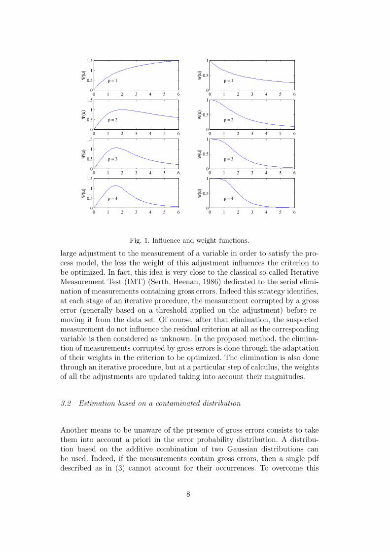
In that case, the associated objective function is much more complex. However,the reader will notice that its expression is not necessary in the consideredcontext. Figure 1 shows the look of the influence function and the weightfunction for some value of p with α = 2.

For p = 1, the influence function is increasing but for p > 1, that function in-creases until a particular value and next decreases. This property explains theability to limit the influence of gross errors onto the estimates. The α parame-ter determines the intermediate zone between increasing and decreasing of theinfluence function. The parameter α must be chosen by the user dependingon an a priori knowledge about the magnitude of the errors (considered asabnormal) which corrupt the measurements.

The ability to limit the influence of gross errors can also be explained lookingat the weight function. Indeed, the more the estimation procedure applies a

7

0 1 2 3 4 5 60

0.5

1

1.5

p = 1Ψ(u

)

0 1 2 3 4 5 60

0.5

1

p = 1w(u

)

0 1 2 3 4 5 60

0.5

1

1.5

p = 2Ψ(u

)

0 1 2 3 4 5 60

0.5

1

p = 2w(u

)

0 1 2 3 4 5 60

0.5

1

1.5

p = 3Ψ(u

)

0 1 2 3 4 5 60

0.5

1

p = 3w(u

)

0 1 2 3 4 5 60

0.5

1

1.5

p = 4Ψ(u

)

0 1 2 3 4 5 60

0.5

1

p = 4w(u

)

Fig. 1. Influence and weight functions.

large adjustment to the measurement of a variable in order to satisfy the pro-cess model, the less the weight of this adjustment influences the criterion tobe optimized. In fact, this idea is very close to the classical so-called IterativeMeasurement Test (IMT) (Serth, Heenan, 1986) dedicated to the serial elimi-nation of measurements containing gross errors. Indeed this strategy identifies,at each stage of an iterative procedure, the measurement corrupted by a grosserror (generally based on a threshold applied on the adjustment) before re-moving it from the data set. Of course, after that elimination, the suspectedmeasurement do not influence the residual criterion at all as the correspondingvariable is then considered as unknown. In the proposed method, the elimina-tion of measurements corrupted by gross errors is done through the adaptationof their weights in the criterion to be optimized. The elimination is also donethrough an iterative procedure, but at a particular step of calculus, the weightsof all the adjustments are updated taking into account their magnitudes.

3.2 Estimation based on a contaminated distribution

Another means to be unaware of the presence of gross errors consists to takethem into account a priori in the error probability distribution. A distribu-tion based on the additive combination of two Gaussian distributions canbe used. Indeed, if the measurements contain gross errors, then a single pdfdescribed as in (3) cannot account for their occurrences. To overcome this

8

problem let us assume that measurement noise is sampled from two pdf, thenormal one having a small variance representing regular noise and the abnor-mal one other having a large variance representing outliers (Wang, Romagnoli,2002),(Ghosh-Dastider, Schafer, 2003). In a first approach, each measurementxi is assumed to have the same normal σ1 and abnormal σ2 standard devia-tions; this hypothesis will be released later on. Thus, for each observation xi,the two following pdf (j = 1, 2) are defined:

pj,i(xi | xi, σj) =1√

2πσj

exp

−1

2

(

xi − xi

σj

)2

(17)

The so-called contaminated pdf is then obtained using a combination of thesetwo pdf:

p(xi | xi, θ) = η p1,i + (1 − η) p2,i, 0 ≤ η ≤ 1 (18)

The vector θ collects the standard deviations σ1 and σ2. The quantity (1 −η) can be seen as an a priori probability of the occurrence of gross errors.Assuming the independence of the measurements, the log-likelihood functionof the measurement set is then written as:

Φ = lnv∏

i=1

p(xi | xi, θ) (19)

As previously said, the best estimate x (in the maximum likelihood sense) ofthe state vector x is obtained by maximizing the log-likelihood function withrespect to x subject to the model constraints:

x = arg maxx

lnv∏

i=1

p(xi | xi, θ) (20a)

subject to Ax = 0 (20b)

The corresponding Lagrange function associated to this optimization problemis written as follows:

L =v∑

i=1

ln p(xi | xi, θ) + λT Ax (21)

The partial derivatives of this Lagrange function with regard to the unknownvariables x and λ must therefore be evaluated. It is easy to establish that:

∂ ln p(xi | xi, θ)

∂xi=

ησ21p1,i + 1−η

σ22

p2,i

η p1,i + (1 − η) p2,i(xi − xi) (22)

9

Therefore, the estimate x is the solution of the following system:

∂L∂x

∣

∣

∣

x=x= W−1

x (x − x) + AT λ = 0

∂L∂λ

∣

∣

∣

x=x= Ax = 0

(23)

with:

W−1x = diag

i=1..v

ησ21p1,i + 1−η

σ22

p2,i

η p1,i + (1 − η) p2,i

(24a)

pj,i =1√

2πσj

exp

−1

2

(

xi − xi

σj

)2

(24b)

Clearly, the obtained system of equations defining the estimate (23) is exacltythe same as that obtained previously using the generalized maximum likeli-hood objective function (11). The only difference concerns the definition ofthe weight matrix W−1

x . Following the resolution method introduced in theprevious section, the following direct iterative scheme is proposed for solvingthis nonlinear system (23):

k = 0, x(k) = x (25a)

p(k)j,i =

1√2πσj

exp

−1

2

x(k)i − xi

σj

2

(25b)

(W(k)x )−1 = diag

i=1..v

ησ21p

(k)1,i + 1−η

σ22

p(k)2,i

η p(k)1,i + (1 − η) p

(k)2,i

(25c)

x(k+1) =(

I − W(k)x AT (AW

(k)x AT )−1A

)

x (25d)

Clearly, representing gross errors by random variables with centered probabil-ity density functions can appear as a complete contradiction with the definitionof what a gross error is. If so, gross errors are then only considered as normalerrors with high variance and low probability. However, this trick that hasbeen already used by other authors, even if it don’t really describe the situa-tion, allows the construction of a robust estimator. The main idea is already togive a small weight, in the criterion to be minimized, to the large adjustments(differences between estimate and measurement). Indeed, this approach limitsthe “smearing” caused by the occurrence of a gross error on the estimates ofother process variables.

Let us now analyze the behavior of the weight function introduced in (22)and explain how the proposed estimation method is able to reject the data

10

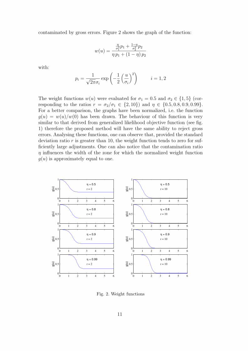
contaminated by gross errors. Figure 2 shows the graph of the function:

w(u) =

ησ21p1 + 1−η

σ22

p2

η p1 + (1 − η) p2

with:

pi =1√2πσi

exp

(

−1

2

(

u

σi

)2)

i = 1, 2

The weight functions w(u) were evaluated for σ1 = 0.5 and σ2 ∈ {1, 5} (cor-responding to the ratios r = σ2/σ1 ∈ {2, 10}) and η ∈ {0.5, 0.8, 0.9, 0.99}.For a better comparison, the graphs have been normalized, i.e. the functiong(u) = w(u)/w(0) has been drawn. The behaviour of this function is verysimilar to that derived from generalized likelihood objective function (see fig.1) therefore the proposed method will have the same ability to reject grosserrors. Analysing these functions, one can observe that, provided the standarddeviation ratio r is greater than 10, the weight function tends to zero for suf-ficiently large adjustments. One can also notice that the contamination ratioη influences the width of the zone for which the normalized weight functiong(u) is approximately equal to one.

0 1 2 3 4 5 60

0.5

1

η = 0.5

r = 2g(u)

0 1 2 3 4 5 60

0.5

1

η = 0.5

r = 10g(u)

0 1 2 3 4 5 60

0.5

1

η = 0.8

r = 2g(u)

0 1 2 3 4 5 60

0.5

1

η = 0.8

r = 10g(u)

0 1 2 3 4 5 60

0.5

1

η = 0.9

r = 2g(u)

0 1 2 3 4 5 60

0.5

1

η = 0.9

r = 10g(u)

0 1 2 3 4 5 60

0.5

1

η = 0.99

r = 2g(u)

0 1 2 3 4 5 60

0.5

1

η = 0.99

r = 10g(u)

Fig. 2. Weight functions

11

4 Extension to bilinear systems

We consider now the case of a process characterised by two types of variables:macroscopic variables such as flowrates x and microscopic variables such con-centrations or mineral species yc, c = 1..q. As for the linear case, measurementnoise is sampled from two pdf, one having a small variance representing regu-lar noise and the other having a large variance representing biases. In order tosimplify the presentation, each measurement xi (resp. yc,i) is assumed to havethe same normal σx,1 (resp. σyc,1) and abnormal σx,2 (resp. σyc,2) standard-deviations. As previously mentioned, this hypothesis will be withdrawn lateron. Thus, for each observation xi and yc,i, the following pdf are defined:

p(xi|xi, σx,j) =1√

2πσx,j

exp

−1

2

(

xi − xi

σx,j

)2

(26a)

p(yc,i|yc,i, σyc,j) =1√

2πσyc,j

exp

−1

2

(

yc,i − yc,i

σyc,j

)2

(26b)

with j = 1, 2, i = 1..v, c = 1..q. In the following, px,j,i and pyc,j,i are shorten-ing notations for p(xi|xi, σx,j) and p(yc,i|yc,i, σyc,j) where indexes i and j arerespectively used to point the number of data and the number of the dis-tribution. As for the linear case, the contaminated pdf of the two types ofmeasurements are defined:

px,i = η1 px,1,i + (1 − η1) px,2,i (27a)

pyc,i = η2 pyc,1,i + (1 − η2) pyc,2,i (27b)

In order to simplify the presentation, all the distributions describing the yc,i

variables have been chosen identical i.e. with the same contamination ratioη2. Assuming independence of the measurements allows the definition of theglobal log-likelihood function:

Φ = lnv∏

i=1

(

px,i

q∏

c=1

pyc,i

)

(28)

Mass balance constraints for total flowrates and partial flowrates are writtenusing the operator ⊗ used to perform the element by element product of twovectors:

Ax = 0 (29)

A(x ⊗ yc) = 0, c = 1..q (30)

12

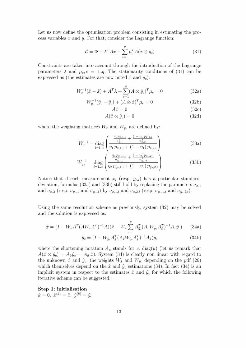
Let us now define the optimisation problem consisting in estimating the pro-cess variables x and y. For that, consider the Lagrange function:

L = Φ + λT Ax +q∑

c=1

µTc A(x ⊗ yc) (31)

Constraints are taken into account through the introduction of the Lagrangeparameters λ and µc, c = 1..q. The stationarity conditions of (31) can beexpressed as (the estimates are now noted x and yc):

W−1x (x − x) + AT λ +

q∑

c=1

(A ⊗ yc)T µc = 0 (32a)

W−1yc

(yc − yc) + (A ⊗ x)T µc = 0 (32b)

Ax = 0 (32c)

A(x ⊗ yc) = 0 (32d)

where the weighting matrices Wx and Wycare defined by:

W−1x = diag

i=1..v

η1 px,1,i

σ2x,1

+(1−η1) px,2,i

σ2x,2

η1 px,1,i + (1 − η1) px,2,i

(33a)

W−1yc

= diagi=1..v

η2 pyc,1,i

σ2yc,1

+(1−η2) pyc,2,i

σ2yc,2

η2 pyc,1,i + (1 − η2) pyc,2,i

(33b)

Notice that if each measurement xi (resp. yc,i) has a particular standard-deviation, formulas (33a) and (33b) still hold by replacing the parameters σx,1

and σx,2 (resp. σyc,1 and σyc,2) by σx,1,i and σx,2,i (resp. σyc,1,i and σyc,2,i).

Using the same resolution scheme as previously, system (32) may be solvedand the solution is expressed as:

x = (I − WxAT (AWxA

T )−1A)(x − Wx

q∑

c=1

ATyc

(AxWycAT

x )−1Axyc) (34a)

yc = (I − WycAT

x (AxWycAT

x )−1Ax)yc (34b)

where the shortening notation Au stands for A diag(u) (let us remark thatA(x ⊗ yc) = Axyc = Ayc

x). System (34) is clearly non linear with regard tothe unknown x and yc, the weights Wx and Wyc

depending on the pdf (26)which themselves depend on the x and yc estimations (34). In fact (34) is animplicit system in respect to the estimates x and yc for which the followingiterative scheme can be suggested:

Step 1: initialisation

k = 0, x(k) = x, y(k) = yc

13

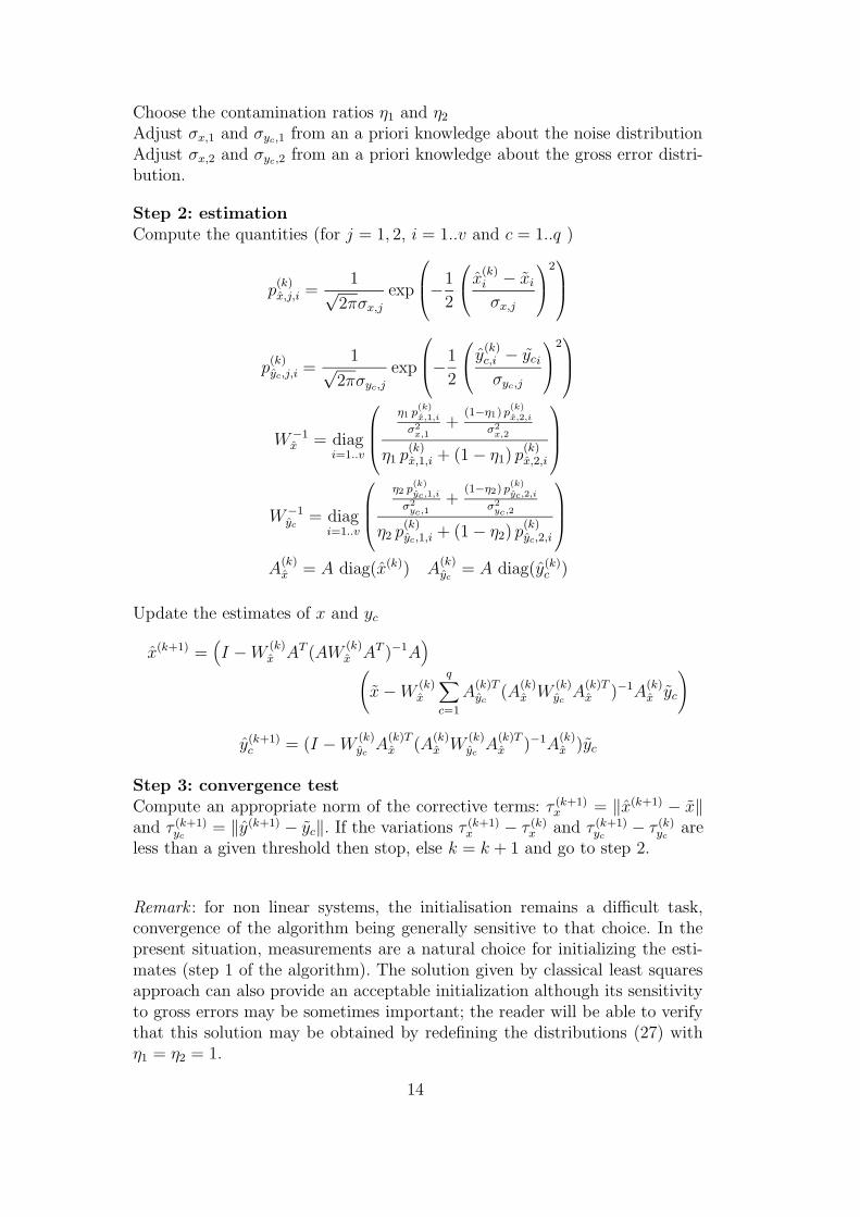
Choose the contamination ratios η1 and η2

Adjust σx,1 and σyc,1 from an a priori knowledge about the noise distributionAdjust σx,2 and σyc,2 from an a priori knowledge about the gross error distri-bution.

Step 2: estimation

Compute the quantities (for j = 1, 2, i = 1..v and c = 1..q )

p(k)x,j,i =

1√2πσx,j

exp

−1

2

x(k)i − xi

σx,j

2

p(k)yc,j,i =

1√2πσyc,j

exp

−1

2

y(k)c,i − yci

σyc,j

2

W−1x = diag

i=1..v

η1 p(k)x,1,i

σ2x,1

+(1−η1) p

(k)x,2,i

σ2x,2

η1 p(k)x,1,i + (1 − η1) p

(k)x,2,i

W−1yc

= diagi=1..v

η2 p(k)yc,1,i

σ2yc,1

+(1−η2) p

(k)yc,2,i

σ2yc,2

η2 p(k)yc,1,i + (1 − η2) p

(k)yc,2,i

A(k)x = A diag(x(k)) A

(k)yc

= A diag(y(k)c )

Update the estimates of x and yc

x(k+1) =(

I − W(k)x AT (AW

(k)x AT )−1A

)

(

x − W(k)x

q∑

c=1

A(k)Tyc

(A(k)x W

(k)yc

A(k)Tx )−1A

(k)x yc

)

y(k+1)c = (I − W

(k)yc

A(k)Tx (A

(k)x W

(k)yc

A(k)Tx )−1A

(k)x )yc

Step 3: convergence test

Compute an appropriate norm of the corrective terms: τ (k+1)x = ‖x(k+1) − x‖

and τ (k+1)yc

= ‖y(k+1) − yc‖. If the variations τ (k+1)x − τ (k)

x and τ (k+1)yc

− τ (k)yc

areless than a given threshold then stop, else k = k + 1 and go to step 2.

Remark : for non linear systems, the initialisation remains a difficult task,convergence of the algorithm being generally sensitive to that choice. In thepresent situation, measurements are a natural choice for initializing the esti-mates (step 1 of the algorithm). The solution given by classical least squaresapproach can also provide an acceptable initialization although its sensitivityto gross errors may be sometimes important; the reader will be able to verifythat this solution may be obtained by redefining the distributions (27) withη1 = η2 = 1.

14

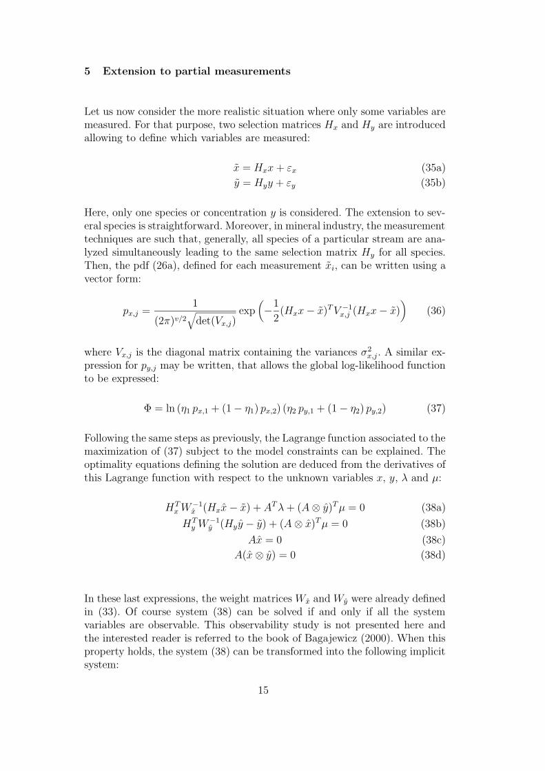
5 Extension to partial measurements

Let us now consider the more realistic situation where only some variables aremeasured. For that purpose, two selection matrices Hx and Hy are introducedallowing to define which variables are measured:

x = Hxx + εx (35a)

y = Hyy + εy (35b)

Here, only one species or concentration y is considered. The extension to sev-eral species is straightforward. Moreover, in mineral industry, the measurementtechniques are such that, generally, all species of a particular stream are ana-lyzed simultaneously leading to the same selection matrix Hy for all species.Then, the pdf (26a), defined for each measurement xi, can be written using avector form:

px,j =1

(2π)v/2√

det(Vx,j)exp

(

−1

2(Hxx − x)T V −1

x,j (Hxx − x))

(36)

where Vx,j is the diagonal matrix containing the variances σ2x,j. A similar ex-

pression for py,j may be written, that allows the global log-likelihood functionto be expressed:

Φ = ln (η1 px,1 + (1 − η1) px,2) (η2 py,1 + (1 − η2) py,2) (37)

Following the same steps as previously, the Lagrange function associated to themaximization of (37) subject to the model constraints can be explained. Theoptimality equations defining the solution are deduced from the derivatives ofthis Lagrange function with respect to the unknown variables x, y, λ and µ:

HTx W−1

x (Hxx − x) + AT λ + (A ⊗ y)T µ = 0 (38a)

HTy W−1

y (Hyy − y) + (A ⊗ x)T µ = 0 (38b)

Ax = 0 (38c)

A(x ⊗ y) = 0 (38d)

In these last expressions, the weight matrices Wx and Wy were already definedin (33). Of course system (38) can be solved if and only if all the systemvariables are observable. This observability study is not presented here andthe interested reader is referred to the book of Bagajewicz (2000). When thisproperty holds, the system (38) can be transformed into the following implicitsystem:

15

x =(

Gx − GxAT (AGxA

T )−1AGx

) (

HTx W−1

x x − ATy (AxGyA

Tx )−1AxGyH

Ty W−1

y y)

(39a)

y = (Gy − GyATx (AxGyA

Tx )−1AxGy)H

Ty W−1

y y (39b)

Gx = (HTx W−1

x Hx + AT A)−1 (39c)

Gy = (HTy W−1

y Hy + ATx Ax)

−1 (39d)

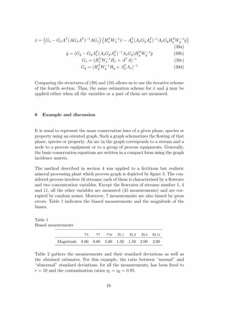
Comparing the structures of (39) and (34) allows us to use the iterative schemeof the fourth section. Thus, the same estimation scheme for x and y may beapplied either when all the variables or a part of them are measured.

6 Example and discussion

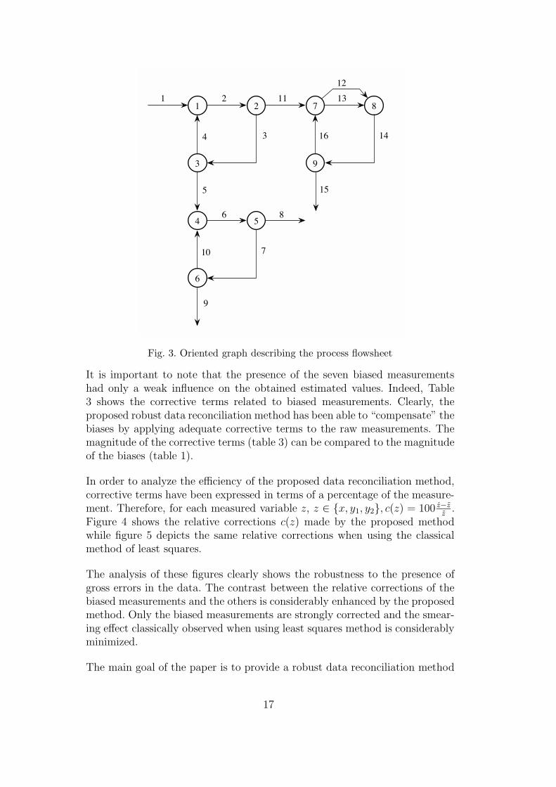
It is usual to represent the mass conservation laws of a given phase, species orproperty using an oriented graph. Such a graph schematizes the flowing of thatphase, species or property. An arc in the graph corresponds to a stream and anode to a process equipment or to a group of process equipments. Generally,the basic conservation equations are written in a compact form using the graphincidence matrix.

The method described in section 4 was applied to a fictitious but realisticmineral processing plant which process graph is depicted by figure 3. The con-sidered process involves 16 streams; each of them is characterized by a flowrateand two concentration variables. Except the flowrates of streams number 1, 4and 11, all the other variables are measured (45 measurements) and are cor-rupted by random noises. Moreover, 7 measurements are also biased by grosserrors. Table 1 indicates the biased measurements and the magnitude of thebiases.

Table 1Biased measurements

x3 x7 x16 y1,1 y1,9 y2,8 y2,14

Magnitude 8.00 8.00 5.00 1.50 1.50 2.00 2.00

Table 2 gathers the measurements and their standard deviations as well asthe obtained estimates. For this example, the ratio between “normal” and“abnormal” standard deviations, for all the measurements, has been fixed tor = 10 and the contamination ratios η1 = η2 = 0.95.

16

1 2 7 8

3 9

4 5

6

2 11 13

1634

5

6

10

14

7

1

15

8

9

12

Fig. 3. Oriented graph describing the process flowsheet

It is important to note that the presence of the seven biased measurementshad only a weak influence on the obtained estimated values. Indeed, Table3 shows the corrective terms related to biased measurements. Clearly, theproposed robust data reconciliation method has been able to “compensate” thebiases by applying adequate corrective terms to the raw measurements. Themagnitude of the corrective terms (table 3) can be compared to the magnitudeof the biases (table 1).

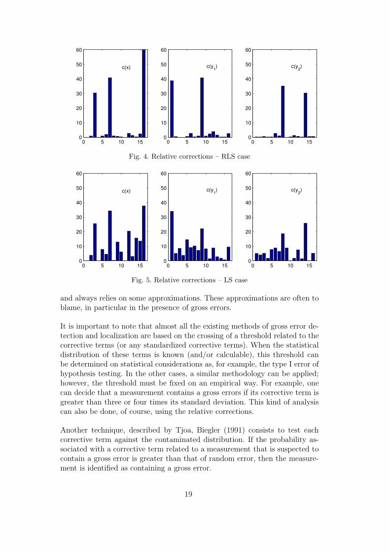
In order to analyze the efficiency of the proposed data reconciliation method,corrective terms have been expressed in terms of a percentage of the measure-ment. Therefore, for each measured variable z, z ∈ {x, y1, y2}, c(z) = 100 z−z

z.

Figure 4 shows the relative corrections c(z) made by the proposed methodwhile figure 5 depicts the same relative corrections when using the classicalmethod of least squares.

The analysis of these figures clearly shows the robustness to the presence ofgross errors in the data. The contrast between the relative corrections of thebiased measurements and the others is considerably enhanced by the proposedmethod. Only the biased measurements are strongly corrected and the smear-ing effect classically observed when using least squares method is considerablyminimized.

The main goal of the paper is to provide a robust data reconciliation method

17

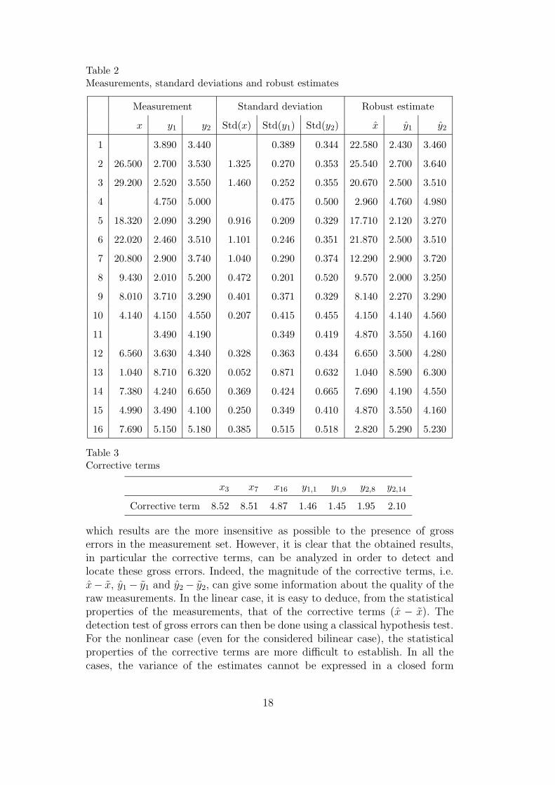
Table 2Measurements, standard deviations and robust estimates

Measurement Standard deviation Robust estimate

x y1 y2 Std(x) Std(y1) Std(y2) x y1 y2

1 3.890 3.440 0.389 0.344 22.580 2.430 3.460

2 26.500 2.700 3.530 1.325 0.270 0.353 25.540 2.700 3.640

3 29.200 2.520 3.550 1.460 0.252 0.355 20.670 2.500 3.510

4 4.750 5.000 0.475 0.500 2.960 4.760 4.980

5 18.320 2.090 3.290 0.916 0.209 0.329 17.710 2.120 3.270

6 22.020 2.460 3.510 1.101 0.246 0.351 21.870 2.500 3.510

7 20.800 2.900 3.740 1.040 0.290 0.374 12.290 2.900 3.720

8 9.430 2.010 5.200 0.472 0.201 0.520 9.570 2.000 3.250

9 8.010 3.710 3.290 0.401 0.371 0.329 8.140 2.270 3.290

10 4.140 4.150 4.550 0.207 0.415 0.455 4.150 4.140 4.560

11 3.490 4.190 0.349 0.419 4.870 3.550 4.160

12 6.560 3.630 4.340 0.328 0.363 0.434 6.650 3.500 4.280

13 1.040 8.710 6.320 0.052 0.871 0.632 1.040 8.590 6.300

14 7.380 4.240 6.650 0.369 0.424 0.665 7.690 4.190 4.550

15 4.990 3.490 4.100 0.250 0.349 0.410 4.870 3.550 4.160

16 7.690 5.150 5.180 0.385 0.515 0.518 2.820 5.290 5.230

Table 3Corrective terms

x3 x7 x16 y1,1 y1,9 y2,8 y2,14

Corrective term 8.52 8.51 4.87 1.46 1.45 1.95 2.10

which results are the more insensitive as possible to the presence of grosserrors in the measurement set. However, it is clear that the obtained results,in particular the corrective terms, can be analyzed in order to detect andlocate these gross errors. Indeed, the magnitude of the corrective terms, i.e.x− x, y1 − y1 and y2 − y2, can give some information about the quality of theraw measurements. In the linear case, it is easy to deduce, from the statisticalproperties of the measurements, that of the corrective terms (x − x). Thedetection test of gross errors can then be done using a classical hypothesis test.For the nonlinear case (even for the considered bilinear case), the statisticalproperties of the corrective terms are more difficult to establish. In all thecases, the variance of the estimates cannot be expressed in a closed form

18

0 5 10 150

10

20

30

40

50

60

c(x)

0 5 10 150

10

20

30

40

50

60

c(y1)

0 5 10 150

10

20

30

40

50

60

c(y2)

Fig. 4. Relative corrections – RLS case

0 5 10 150

10

20

30

40

50

60

c(x)

0 5 10 150

10

20

30

40

50

60

c(y1)

0 5 10 150

10

20

30

40

50

60

c(y2)

Fig. 5. Relative corrections – LS case

and always relies on some approximations. These approximations are often toblame, in particular in the presence of gross errors.

It is important to note that almost all the existing methods of gross error de-tection and localization are based on the crossing of a threshold related to thecorrective terms (or any standardized corrective terms). When the statisticaldistribution of these terms is known (and/or calculable), this threshold canbe determined on statistical considerations as, for example, the type I error ofhypothesis testing. In the other cases, a similar methodology can be applied;however, the threshold must be fixed on an empirical way. For example, onecan decide that a measurement contains a gross errors if its corrective term isgreater than three or four times its standard deviation. This kind of analysiscan also be done, of course, using the relative corrections.

Another technique, described by Tjoa, Biegler (1991) consists to test eachcorrective term against the contaminated distribution. If the probability as-sociated with a corrective term related to a measurement that is suspected tocontain a gross error is greater than that of random error, then the measure-ment is identified as containing a gross error.

19

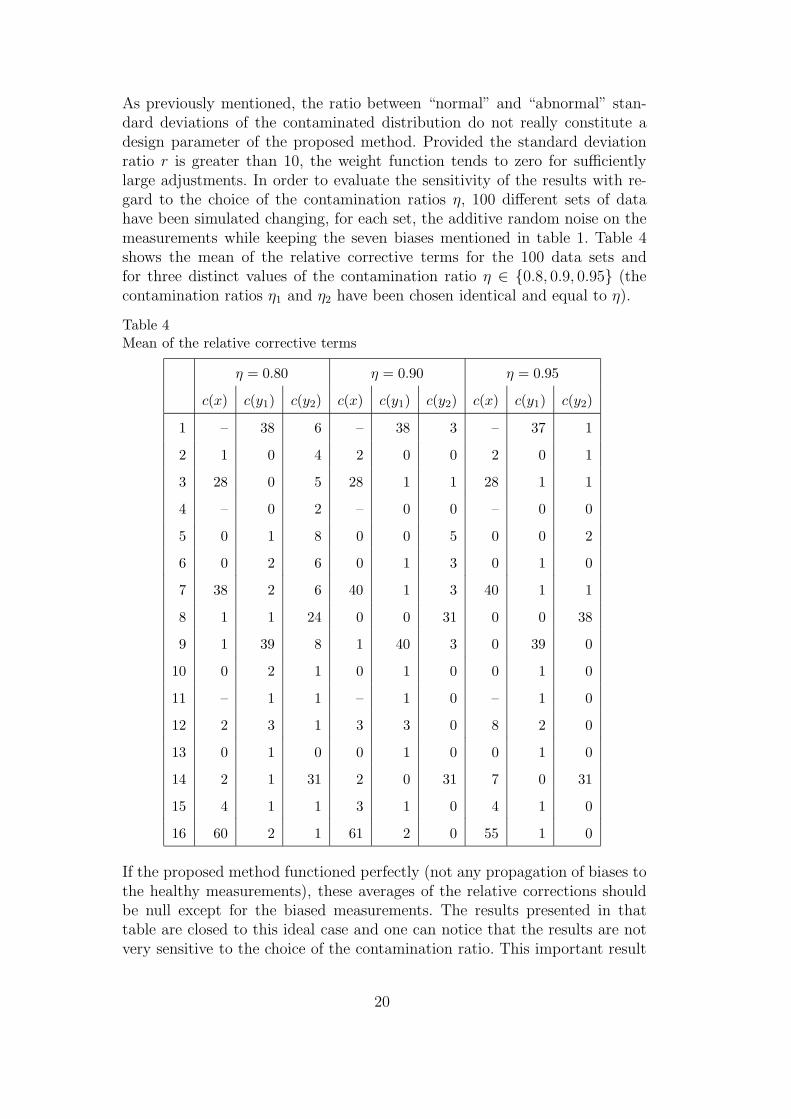
As previously mentioned, the ratio between “normal” and “abnormal” stan-dard deviations of the contaminated distribution do not really constitute adesign parameter of the proposed method. Provided the standard deviationratio r is greater than 10, the weight function tends to zero for sufficientlylarge adjustments. In order to evaluate the sensitivity of the results with re-gard to the choice of the contamination ratios η, 100 different sets of datahave been simulated changing, for each set, the additive random noise on themeasurements while keeping the seven biases mentioned in table 1. Table 4shows the mean of the relative corrective terms for the 100 data sets andfor three distinct values of the contamination ratio η ∈ {0.8, 0.9, 0.95} (thecontamination ratios η1 and η2 have been chosen identical and equal to η).

Table 4Mean of the relative corrective terms

η = 0.80 η = 0.90 η = 0.95

c(x) c(y1) c(y2) c(x) c(y1) c(y2) c(x) c(y1) c(y2)

1 – 38 6 – 38 3 – 37 1

2 1 0 4 2 0 0 2 0 1

3 28 0 5 28 1 1 28 1 1

4 – 0 2 – 0 0 – 0 0

5 0 1 8 0 0 5 0 0 2

6 0 2 6 0 1 3 0 1 0

7 38 2 6 40 1 3 40 1 1

8 1 1 24 0 0 31 0 0 38

9 1 39 8 1 40 3 0 39 0

10 0 2 1 0 1 0 0 1 0

11 – 1 1 – 1 0 – 1 0

12 2 3 1 3 3 0 8 2 0

13 0 1 0 0 1 0 0 1 0

14 2 1 31 2 0 31 7 0 31

15 4 1 1 3 1 0 4 1 0

16 60 2 1 61 2 0 55 1 0

If the proposed method functioned perfectly (not any propagation of biases tothe healthy measurements), these averages of the relative corrections shouldbe null except for the biased measurements. The results presented in thattable are closed to this ideal case and one can notice that the results are notvery sensitive to the choice of the contamination ratio. This important result

20

was foreseeable taking into account the shape of the weight functions shownon figure 2.

7 Conclusion

To deal with the issues of gross errors influence on data estimation, the pa-per has presented a robust reconciliation approach. For that purpose, a costfunction which is less sensitive to the outlying observations than that of leastsquares is used. The algorithm can handle multiple biases or gross errors at atime. For the given example, 7 measurements among 45 have been biased andthe proposed method has been able to provide a good estimation of the truevalues of the different variables of the process. The implementation of the al-gorithm is easy; moreover many simulations carried out showed a relative lowsensitivity of the results to the design parameters, i.e. the standard deviationratio r and the contamination ratio η (provided, of course, these parametersare not completely randomly chosen).

The results of reconciliation will clearly depend not only on the data, but alsoon the model of the process itself. As a perspective of development of robustreconciliation strategies, there is a need for taking account of model uncer-tainties and optimise the balancing parameter w. Moreover, for process withunknown parameters, it should be important to jointly estimate the reconcileddata and the process parameters.

References

Abu-el-zeet, Z.H., Roberts, P.D. and Becerra, V.M. (2001). Bias detection andidentification in dynamic data reconciliation. In European Control Confer-

ence, Porto, Portugal, September 4-7.Arora, N. and Biegler, L.T. (2001). Redescending estimator for data reconcil-

iation and parameter estimation. Computers and Chemical Engineering, 25(11/12), 1585-1599.

Bagajewicz, M.J. Process plant instrumentation: design and upgrade. Lan-caster, PA: Technomic Publishing Company, 2000.

Border, K.C. (1985). Fixed point theorems with applications to economics and

game theory. Cambridge University Press.Crowe, C.M. (1996). Data reconciliation - progress and challenges. Journal of

Process Control, 6 (2/3), 89-98.Dhurjati, P. and Cauvin, S. (1999). On-line fault detection and supervision in

the chemical process industries. Control Engineering Practice, 7 (7), 863-864.

21

Ghosh-Dastider, B. and Schafer, J.L. (2003). Outlier detection and editing pro-cedures for continuous multivariate data. Working paper 2003-07, RAND,Santa Monica OPR, Princeton University.

Hampel, F.R., Ronchetti, E.M., Rousseeuw, P.J. and Stohel, W.A. (1986).Robust statistic: the approach on influence functions. Wiley, New-York.

Heyen, G. (1999). Industrial applications of data reconciliation: operatingcloser to the limits with improved design of the measurement system. InWorkshop on Modelling for Operator Support, Lappeenranta University ofTechnology, June 22.

Himmelblau, D.M. (1978). Fault detection and diagnosis in chemical and petro-

chemical processes. Elsevier Scientific Pub. Co.Hodouin, D. and Flament, F. (1989). New developments in material balance

calculations for mineral processing industry. In Society of Mining Engineers

annual meeting, Las Vegas, February 27 - March 2.Hoffman, J.D. (2001). Numerical methods for engineers and scientists. Marcel

Dekker.Huber, P.J. (1981). Robust statistic. John Wiley & Sons, New York.Johnston, L.PM. and Kramer, M.A. (1995). Maximum likelihood data rectifi-

cation: steady state systems. AIChE Journal, 41(11), 2415-2426.Kim, I., Kang, M.S., Park, S. and Edgar, T.F. (1997). Robust data reconcili-

ation and gross error detection: the modified MIMT using NLP. Computers

and Chemical Engineering, 21, 775-782.Kuehn, D.R. and Davidson, H. (1961). Computer control. II: Mathematics of

control. Chemical Engineering Progress, 57, 44.Mah, R.S.H., Stanley, G.M. and Downing, D. (1976). Reconciliation and rec-

tification of process flow and inventory data. Ind. Eng. Chem., Process Des.

Dev., 15 (1), 175-183.Maquin, D., Bloch, G. and Ragot, J. (1991). Data reconciliation for measure-

ments. European Journal of Diagnosis and Safety in Automation, 1 (2),145-181.

Narasimhan, S. and Jordache, C. (2000). Data reconciliation and gross error

detection – an intelligent use of process data, Gulf Publishing Company,Houston, Texas, USA.

Narasimhan, S. and Mah, R.S.H. (1989). Treatment of general steady stateprocess models in gross error identification. Computers and Chemical Engi-

neering, 13 (7), 851-853.Ozyurt, D.B. and Pike, R.W. (2004). Theory and practice of simultaneous data

reconciliation and gross error detection for chemical processes.Computers

and Chemical Engineering, 28, 381-402.Ragot, J., Maquin, D. and Adrot, O. (1999). LMI approach for data recon-

ciliation. In 38th Conference of Metallurgists, Symposium Optimization and

Control in Minerals, Metals and Materials Processing, Quebec, Canada,August 22-26.

Ragot, J. and Maquin, D. (2004). Reformulation of data reconciliation problemwith unknown-but-bounded errors. Industrial and Engineering Chemistry

22

Research, 43 (6), 1530-1536.Serth, R. and Heenan, W. (1986). Gross error detection and data reconciliation

in steam metering systems. AIChE Journal, 32, 733-742.Singh, S.R., Mittal, N.K. and Sen, P.K. (2001). A novel data reconciliation

and gross error detection tool for the mineral processing industry. Minerals

Engineering, 14 (7), 808-814.Soderstrom, T.A., Himmelblau, D.M. and Edgar, T.F. (2001). A mixed integer

optimization approach for simultaneous data reconciliation and identifica-tion of measurement bias. Control Engineering Pratice, 9 (8), 869-876.

Tjoa, I.B. and Biegler, L.T. (1991). Simultaneous strategy for data reconcilia-tion and gross error analysis. Computer and Chemical Engineering, 15 (10),679-689.

Veverka, V.V. and Madron F. (1997). Material and energy balancing in theprocess industries: from microscopic balances to large plants. Computer-

aided chemical engineering series, vol. 7, Amsterdam, The Netherlands, El-sevier.

Wang, D. and Romagnoli, J.A. (2002). Robust data reconciliation based on ageneralized objective function. In 15th IFAC World Congress on Automatic

Control, Barcelona, Spain, July 21-26.Yi, H.-S., Kim, J. H. and Han, C. (2002). Industrial application of gross error

estimation and data reconciliation to byproduction gases in iron and steelmaking plants. In International Conference on Control, Automation and

Systems, Muju, Korea, October 16-19.

23