Data Processing Approach for Localizing Bio-magnetic Sources in the Brain

arX

iv:0

903.

0859

v1 [

q-bi

o.Q

M]

4 M

ar 2

009

Data Processing Approach for Localizing Bio-magnetic

Sources in the Brain

Hung-I Pai1∗, Chih-Yuan Tseng1†and H.C. Lee1,2,3

1Computational Biology Laboratory1Department of Physics, National Central University, Zhongli, Taiwan 32001

2Graduate Institute of Systems Biology and Bioinformatics

National Central University, Zhongli, Taiwan 320013National Center for Theoretical Sciences, Hsinchu, Taiwan 30043

Abstract

Magnetoencephalography (MEG) provides dynamic spatial-temporal insight of neural activ-ities in the cortex. Because the number of possible sources is far greater than the number ofMEG detectors, the proposition to localize sources directly from MEG data is notoriously ill-posed. Here we develop an approach based on data processing procedures including clustering,forward and backward filtering, and the method of maximum entropy. We show that taking asa starting point the assumption that the sources lie in the general area of the auditory cortex(an area of about 40 mm by 15 mm), our approach is capable of achieving reasonable successin pinpointing active sources concentrated in an area of a few mm’s across, while limiting thespatial distribution and number of false positives.

Keyword : MEG, ill-posed inverse problem, clustering, filtering, maximum entropy

1 Introduction

Magnetoencephalography (MEG) records magnetic fields generated from neurons when the brain isperforming a specific function. Neural activities thus can be noninvasively studied through analyzingthe MEG data. Since the number of neurons (unknowns) are far larger than the number of MEGsensors (knowns) outside the brain, the problem of identifying activated neurons from the magneticdata is ill posed. The problem becomes even more severe when noise is present.

A first and essential step in surpassing the obstacle of ill-posedness is to rely on prior knowledgeof the general area of active current sources producing the MEG data. Often, this prior knowledgeis provided by functional magnetic resonance imaging (fMRI) experiments. The two kinds of exper-iments complement each other, MEG has high temporal resolution (about 10−3s) but poor spatialresolution, whereas fMRI has high spatial resolution [1] but poor temporal resolution (about 1 s).Consider auditory neural activity. FMRI shows that such activity is concentrate in the auditorycortex, two 40 mm by 15 mm areas respectively located on the two sides of the cortex (Fig. 1L). Be-cause of poor temporal resolution, fMRI cannot resolve the rapid successive firing of the (groups of)neurons, instead it shows large areas of the auditory cortex lighting up. Under MEG, the same au-ditory activity will be detected by high time-resolution sensors (Fig. 1R) which however collectivelycover an area (when projected down to the cortex) much greater than the auditory cortex.

∗He is currently working in Industrial Technology Research Institute, Chu Tung, Hsin Chu, Taiwan 310.†He is currently at Department of Oncology, University of Alberta, Edmonton AB T6G 1Z2 Canada.

1

Figure 1: Left, side view of the human cortex; the frontal lobe points to the left. The region ofinterest, the auditory cortex, is marked by the dark rectangular. Right, schematic setup of an MEGexperiment. The occipital lobe (right side in graph) is closer to the sensors because the person beingtested is lying face-up.

Although many methods have been proposed to attack the ill-posed problem, including dipolefitting, minimum-norm-least-square (MNLS) [2], and the maximum entropy method (ME) [3], im-provements have been limited. One reason for this may be that these methods do not properlyinclude anatomic constrains. In this work, we propose a novel approach to analyze noisy MEG databased on ME that pays special attention to obtaining better priors as input to the ME procedureby employing clustering and forward and backward filtering processes that take anatomic constrainsinto consideration. We demonstrate the feasibility of our approach by testing it on several simplecases.

2 The ill-posed inverse problem

Given the set of current sources (dipole strengths) {ri|i = 1, 2, · · · , Nr} at sites {zi|i = 1, 2, · · · , Nr},the magnetic field strength m(x) measured by the sensor at spatial position x is given by,

m(x) =

Nr∑

i=1

A(x)iri + n(x) ≡ A(x) · r + n(x) (1)

where the function A(x)i, which is a function of zi, is derived from the Biot-Savart law in vacuum,n(x) is a noise term, and a hatted symbol denotes an Nr-component vector in source space. Weconsider the case where there are Nm sensors at locations xα, α=1,2,· · · , Nm. To simplify notation,we write m as an Nm-component vector whose αth component is mα=m(xα), similarly for A andn. Then Eq. (1) simplifies to

m = A · r + n (2)

In practice, magnetic field strengths are measured at the Nm sensors and the inverse problem is toobtain the set of Nr dipole strengths ri with Nr >> Nm. The presence of noise raises the level ofdifficulty of the inverse problem.

3 Methods

Human Cortex and MEG Sensors. In typical quantitative brain studies, the approximately1010 neurons in the cortex are simulated by about 2.4×105 current dipoles whose directions are setparallel to the normal of the cortex surface [4, 5]. For this study we focus on the auditory cortex,the area marked by the 40 mm× 15 mm rectangular shown in Fig. 1L that contains 2188 currentdipoles.

In typical MEG experiments the human head is surrounded by a hemispheric tiling of magneticfield sensors called superconducting quantum interference devices (SQUIDS). In the experiment we

2

consider, there are 157 sensors, each composed of a pair of co-axial coils of 15.5 mm diameter 50mm apart, with the lower coil about 50 mm above the scalp [6]. The centers of the sensors arerepresented by the gray dots in Fig. 1R. Details of geometry and of the A-matrixes in Eq. (1) aregiven in [7].

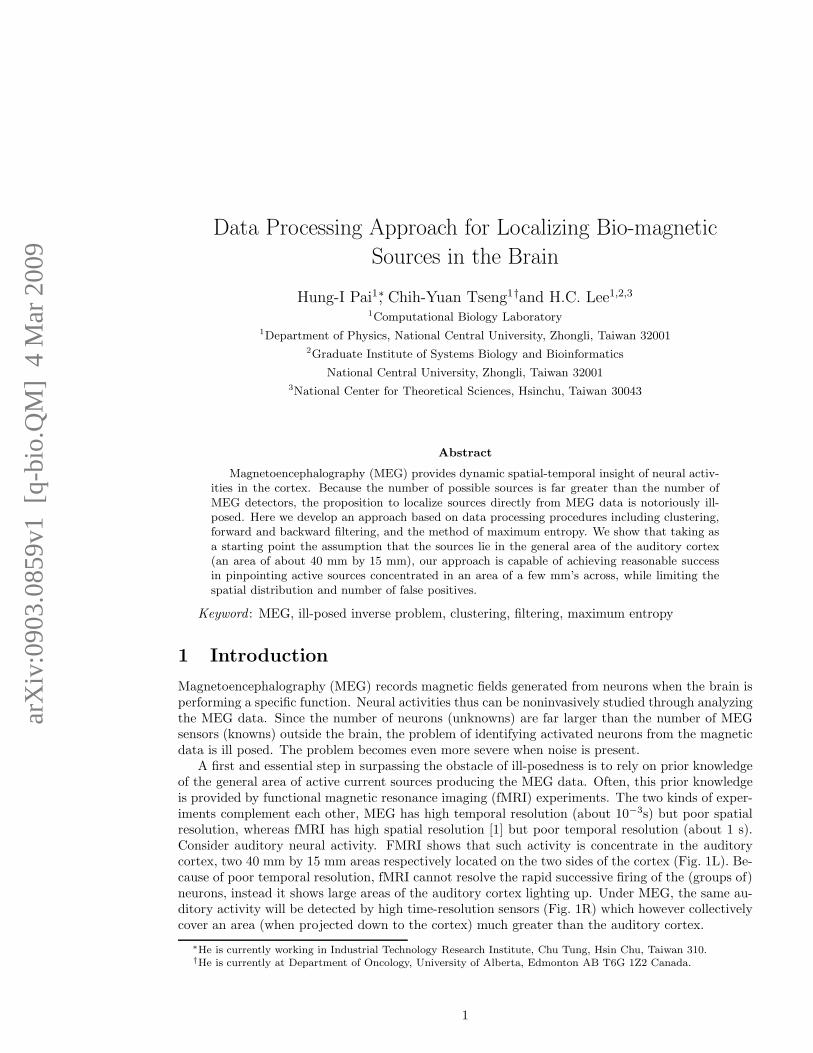
Artificial MEG data and Noise. We use artificial MEG data generated by the forward equa-tion, Eq. (1), from sets of current dipoles (to be specified below) in a small area (black circles inFigs. 2R) within the auditory cortex (the gray ”rectangular” region in Figs. 2L, enlargement shownin Figs. 2R). A site-independent white Gaussian noise is linearly superimposed on the MEG data.

Figure 2: Left, the circular and triangular symbols are the positions of the 31 sensors with detectablesignals, including the 7 (triangular) with signals above threshold. Sensors with magnetic flux goinginto (out) the page are solid (hollow). Right, detail of auditory cortex. The dark (orange in color)circles in the top-right corner indicate the general area of active sources used to generate artificialMEG data.

The signal to noise ratio (SNR) is defined as

SNR = −10log10||nmax||2/||mmax||2 (3)

where mmax is the amplitude at the sensor receiving the strongest noiseless MEG signal, and nmax

is amplitude of the strongest simulated noise. In this study we have mmax=7.4 fT (fT= femto-Tesla)and nmax=0.05mmax=0.37 fT, so that SNR=26 on each individual run. The artificial MEG datais generated by giving a current of 10 nA (nano-ampere) to each of the sources in a source set (seebelow), running the forward equation with noise 10 times and taking the averaged strengths at thesensors. The averaging has the effect of reducing the effective nmax by a factor of

√10, and yielding

an enhanced effective signal to noise ratio of SNR′=36.Using a threshold of TS=14nmax=5.1 fT we select a subset MS of 7 ”strong signal” sensors.

This implies a minimum value of SNR′=32.9 (with averaging) on each sensor in the set. Given the(assumed) normal distribution of noise intensity, this selection implies that at 99.99% confidencelevel the signals considered are not noise. Similarly we use a threshold of TC=6nmax=2.2 fT toselect a subset MC of 31 ”clear signal” sensors, with minimum values of SNR′=25.6 on each sensorin the set. In actual computations below, we reduce the sensor space to one that include only thosein the set MC . In practice, the reduction replaces m, A, and n by m′, A′, and n′, respectively.

Receiver Operating Characteristics Analysis. We evaluate the goodness of our results usingreceiver operating characteristics (ROC) analysis [9], in which the result is presented in the formof a plot of the true positive rate (Sn, sensitivity) versus the false positive rate (or 1-Sp, where Sp

is the specificity). Let R be the total solution space of current sources, T the true solutions, oractual active sources, and P the positives, or the predicted active sources. Then F=R-T is the falsesolutions, TP=(P

⋂T ) the true positives, FP=(P

⋂T )-T the false positives, and FN=R-(P

⋂T )

the false negatives. By definition Sn=TP/T=(P⋂

T )/T and 1-Sp=FP/F=((P⋃

T )−T )/(R−T ).

3

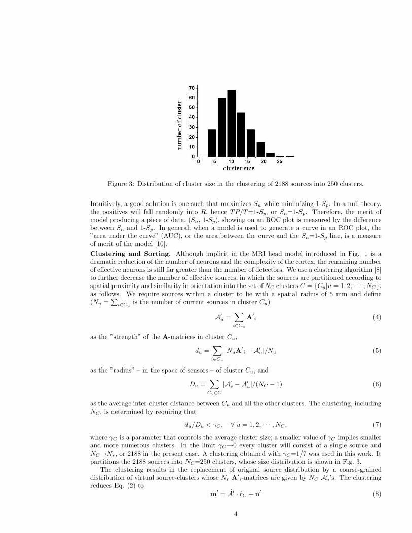
Figure 3: Distribution of cluster size in the clustering of 2188 sources into 250 clusters.

Intuitively, a good solution is one such that maximizes Sn while minimizing 1-Sp. In a null theory,the positives will fall randomly into R, hence TP/T=1-Sp, or Sn=1-Sp. Therefore, the merit ofmodel producing a piece of data, (Sn, 1-Sp), showing on an ROC plot is measured by the differencebetween Sn and 1-Sp. In general, when a model is used to generate a curve in an ROC plot, the”area under the curve” (AUC), or the area between the curve and the Sn=1-Sp line, is a measureof merit of the model [10].

Clustering and Sorting. Although implicit in the MRI head model introduced in Fig. 1 is adramatic reduction of the number of neurons and the complexity of the cortex, the remaining numberof effective neurons is still far greater than the number of detectors. We use a clustering algorithm [8]to further decrease the number of effective sources, in which the sources are partitioned according tospatial proximity and similarity in orientation into the set of NC clusters C = {Cu|u = 1, 2, · · · , NC},as follows. We require sources within a cluster to lie with a spatial radius of 5 mm and define(Nu =

∑i∈Cu

is the number of current sources in cluster Cu)

A′u =

∑

i∈Cu

A′i (4)

as the ”strength” of the A-matrices in cluster Cu,

du =∑

i∈Cu

|NuA′i −A′

u|/Nu (5)

as the ”radius” – in the space of sensors – of cluster Cu, and

Du =∑

Cv∈C

|A′v −A′

u|/(NC − 1) (6)

as the average inter-cluster distance between Cu and all the other clusters. The clustering, includingNC , is determined by requiring that

du/Du < γC , ∀ u = 1, 2, · · · , NC , (7)

where γC is a parameter that controls the average cluster size; a smaller value of γC implies smallerand more numerous clusters. In the limit γC→0 every cluster will consist of a single source andNC→Nr, or 2188 in the present case. A clustering obtained with γC=1/7 was used in this work. Itpartitions the 2188 sources into NC=250 clusters, whose size distribution is shown in Fig. 3.

The clustering results in the replacement of original source distribution by a coarse-graineddistribution of virtual source-clusters whose Nr A′

i-matrices are given by NC A′u’s. The clustering

reduces Eq. (2) tom′ = A′ · rC + n′ (8)

4

which has the same form as Eq. (2) except that here the hatted vectors have only NC componentsand each of NC components in rC denotes the strength of the current dipole representing a cluster.

It is convenient to sort the cluster set C according to the field strength of the clusters. Since thefield strength depends on the where it is measured, the sorted order will be sensor-dependent. Wedenote the sorted set for sensor α by C{α}. Thus we have:

C{α} = {Cuα|uα = 1, 2, · · · , NC}, |A′

uα| ≥ |A′

vα| if uα < vα, ∀α ∈ MC . (9)

Forward Filtering. A key in improving the quality of the solution of an inverse problem is toreduce the number of false positives. In the MEG experiments under consideration, the plane ofthe sensors are generally parallel to the enveloping surface of the cerebral cortex. Such sensors aremeant to detect signals emitted from current sources in sulci on the cortex, and are not sensitiveto signals from sources in gyri. In practice, in our test cases T will be composed of sulcus sources.Therefore, if we simply remove those clusters having the weakest strengths, we will reduce FP at ahigher rate than TP .

Given a positive fractional number ξ < 1, we use it to set an integer number Nξ < NC , and useNξ to define the truncated sets

R{α}ξ = {Cuα

|uα = 1, 2, · · · , Nξ}, ∀ α ∈ MS . (10)

The integer Nξ is determined by regression by demanding the union set

Rξ =⋃

α∈MS

R{α}ξ = ξR (11)

to be a fraction ξ of R. We call this forward filtering process of reducing the pool of possiblepositives from R to Rξ the mostly sulcus model (MSM). About 25% of current sources in R lie ingyri. Therefore, if we set ξ=0.75, very few potentially true sources will be left out. It turns out thatin the region where 1-Sp is only slightly less than unity, setting P to Rξ can offer the best result.

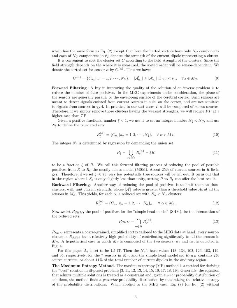
Backward Filtering. Another way of reducing the pool of positives is to limit them to thoseclusters, with unit current strength, whose |A′| value is greater than a threshold value A0 at all thesensors in MS. This yields, for each α, a reduced set with Nα < NC clusters:

R{α}> = {Cuα

|uα = 1, 2, · · · , Nα}α, ∀ α ∈ MS . (12)

Now we let RSHM , the pool of positives for the ”simple head model” (SHM), be the intersection ofthe reduced sets,

RSHM =⋂

α∈M

R{α}> . (13)

RSHM represents a coarse-grained, simplified cortex tailored to the MEG data at hand: every source-cluster in RSHM has a relatively high probability of contributing significantly to all the sensors inMS. A hypothetical case in which MS is composed of the two sensors, α1 and α2, is depicted inFig. 4.

For this paper A0 is set to be 4.5 fT. Then the Nα’s have values 113, 134, 102, 126, 103, 119,and 64, respectively, for the 7 sensors in MS , and the simple head model set RSHM contains 240source currents, or about 11% of the total number of current dipoles in the auditory region.

The Maximum Entropy Method. The maximum entropy (ME) method is a method for derivingthe ”best” solution in ill-posed problems [3, 11, 12, 13, 14, 15, 16, 17, 18, 19]. Generally, the equationthat admits multiple solutions is treated as a constraint and, given a prior probability distribution ofsolutions, the method finds a posterior probability distribution by maximizing the relative entropyof the probability distributions. When applied to the MEG case, Eq. (8) (or Eq. (2) without

5

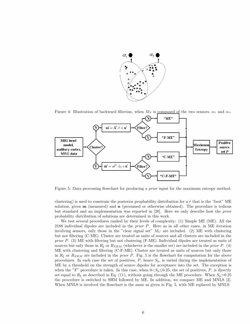
Figure 4: Illustration of backward filtering, when MS is composed of the two sensors, α1 and α2.Both R{α1} and R{α2} contain 3 clusters while RSHM contains only one cluster.

Figure 5: Data processing flowchart for producing a prior input for the maximum entropy method.

clustering) is used to constrain the posterior propbability distribution for a r that is the “best” MEsolution, given m (measured) and n (presumed or otherwise obtained). The procedure is tediousbut standard and an implementation was reported in [20]. Here we only describe how the prior

probability distribution of solutions are determined in this work.We test several procedures ranked by their levels of complexity: (1) Simple ME (ME). All the

2188 individual dipoles are included in the prior P . Here as in all other cases, in ME iterationinvolving sensors, only those in the ”clear signal set” MC are included. (2) ME with clusteringbut not filtering (C-ME). Cluster are treated as units of sources and all clusters are included in theprior P . (3) ME with filtering but not clustering (F-ME). Individual dipoles are treated as units ofsources but only those in Rξ or RSHM (whichever is the smaller set) are included in the prior P . (4)ME with clustering and filtering (C-F-ME). Cluster are treated as units of sources but only thosein Rξ or RSHM are included in the prior P . Fig. 5 is the flowchart for computation for the aboveprocedures. In each case the set of positives, P , hence Sp, is varied during the implementation ofME by a threshold on the strength of source dipoles for acceptance into the set. The exception iswhen the ”F” procedure is taken. In this case, when 0<Sp≤0.25, the set of positives, P , is directlyset equal to Rξ as described in Eq. (11), without going through the ME procedure. When Sp>0.25the procedure is switched to SHM followed by ME. In addition, we compare ME and MNLS [2].When MNLS is involved the flowchart is the same as given in Fig. 5, with ME replaced by MNLS.

6

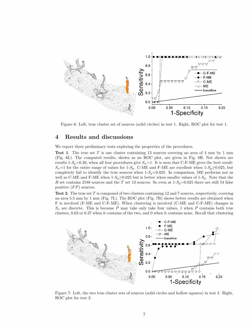
Figure 6: Left, true cluster set of sources (solid circles) in test 1. Right, ROC plot for test 1.

4 Results and discussions

We report three preliminary tests exploring the properties of the procedures.

Test 1. The true set T is one cluster containing 13 sources covering an area of 4 mm by 1 mm(Fig. 6L). The computed results, shown as an ROC plot, are given in Fig. 6R. Not shown areresults 1-Sp>0.20, when all four procedures give Sn=1. It is seen that C-F-ME gives the best result:Sn=1 for the entire range of values for 1-Sp. C-ME and F-ME are excellent when 1-Sp≥0.025, butcompletely fail to identify the true sources when 1-Sp<0.025. In comparison, ME performs not aswell as C-ME and F-ME when 1-Sp≥0.025 but is better when smaller values of 1-Sp. Note that theR set contains 2188 sources and the T set 13 sources. So even at 1-Sp=0.025 there are still 54 falsepositive (FP ) sources.

Test 2. The true set T is composed of two clusters containing 12 and 7 sources, respectively, coveringan area 5.5 mm by 1 mm (Fig. 7L). The ROC plot (Fig. 7R) shows better results are obtained whenF is involved (F-ME and C-F-ME). When clustering is involved (C-ME and C-F-ME) changes inSn are discrete. This is because P may take only take four values, 1 when P contains both trueclusters, 0.63 or 0.37 when it contains of the two, and 0 when it contains none. Recall that clustering

Figure 7: Left, the two true cluster sets of sources (solid circles and hollow squares) in test 2. Right,ROC plot for test 2.

7

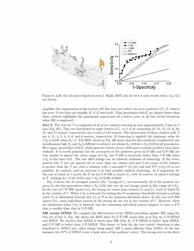
Figure 8: Left, the 42 source dipoles in test 3. Right, ROC plot for test 3; only results with 1-Sp<0.2are shown.

simplifies the organization of the sources (R) but does not reduce the prior positives (P ). F reducesthe prior P but does not simplify R. C-F does both. That procedures with F are clearly better thanthose without highlights the paramount importance of a better prior in all but trivial situationswhen ME is employed.

Test 3. The true set T is composed of 42 active sources covering an area approximately 3 mm by 2mm (Fig. 8L). They are distributed in eight clusters (Cu, u=1 to 8) containing 18, 31, 15, 12, 9, 23,18, and 17 sources, respectively, for a total of 143 sources. The intersection of these clusters with Tare 4, 11, 4, 3, 4, 4, 6, and 6 sources, respectively. If clustering is applied, the minimum value for1-Sp is 0.047 when Sn=1. The ROC shown in Fig. 8R shows that for this relatively complicated casesimultaneous high Sn and Sp is difficult to achieve; we obtain Sn<0.6 for 1-Sp<0.20 in all procedures.Here again, procedures with F, which generate better priors, yield more accurate positives than thosewithout. It is worth pointing out the accuracies of the positives given by F-ME and C-F-ME arevery similar in almost the entire range of 1-Sp, but F-ME is decisively better than C-F-ME when1-Sp is less than 0.01. The last effect brings out an inherent weakness of clustering. If the activesources (the T set) are spread out in more than one cluster and and if the union of the clustersis greater than the T set, then a solution with a non-null P (Sn 6=0) and null FP (1-Sp=0) is notpossible. In contrast, such an outcome is at least possible without clustering. As it happened, forthe case at hand, at 1-Sp≈0, the P set for C-F-ME is cluster C4 with 12 sources, of which 3 belongsto T , yielding Sn=3/42=0.071 and 1-Sp=9/2146=0.0042.

Fig. 9 shows the 21 strongest sources (the ”strong set”), not necessarily all in the positive set,given by the four procedures when 1-Sp<0.02 (the sets do not change much in this range of 1-Sp).In the case of C-F-ME (panel (a)), the strong set comes from clusters C3 and C4, both of which liein the vicinity of T . When 1-Sp is lowered (by raising the P -acceptance threshold) beyond a certainpoint C3 is eliminated, leaving only C4 in P in the situation discussed above. In the case of F-ME(panel (b)), some individual sources in the strong set are not in the vicinity of T . However, theseare eliminated when 1-Sp is lowered, and the remaining individual sources happen to have a FPthat is smaller than that in C-F-ME.

ME versus MNLS. We compare the effectiveness of the MNLS procedure against ME using thetrue set of test 3. Fig. 10L shows the ROC plots for C-F-ME (same plot as in Fig. 8), C-F-MNLSand MNLS. We observe that MNLS is worse than ME (Fig. 8), C-F-MNLS is better than MNLS,and C-F-ME is better than C-F-MNLS. This shows, at least for the case tested, clustering is alsobeneficial to MNLS and, other things being equal, ME is more effective than MNLS. In the lastinstance the FP ’s of MNLS cover a large area of the auditory cortex. The strong sets in the three

8

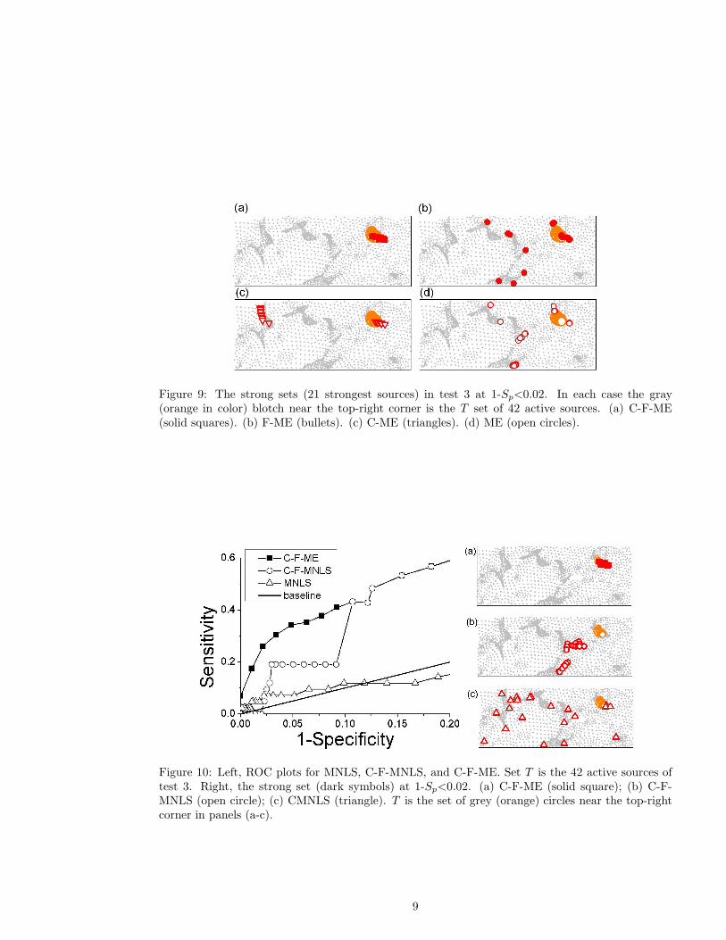
Figure 9: The strong sets (21 strongest sources) in test 3 at 1-Sp<0.02. In each case the gray(orange in color) blotch near the top-right corner is the T set of 42 active sources. (a) C-F-ME(solid squares). (b) F-ME (bullets). (c) C-ME (triangles). (d) ME (open circles).

Figure 10: Left, ROC plots for MNLS, C-F-MNLS, and C-F-ME. Set T is the 42 active sources oftest 3. Right, the strong set (dark symbols) at 1-Sp<0.02. (a) C-F-ME (solid square); (b) C-F-MNLS (open circle); (c) CMNLS (triangle). T is the set of grey (orange) circles near the top-rightcorner in panels (a-c).

9

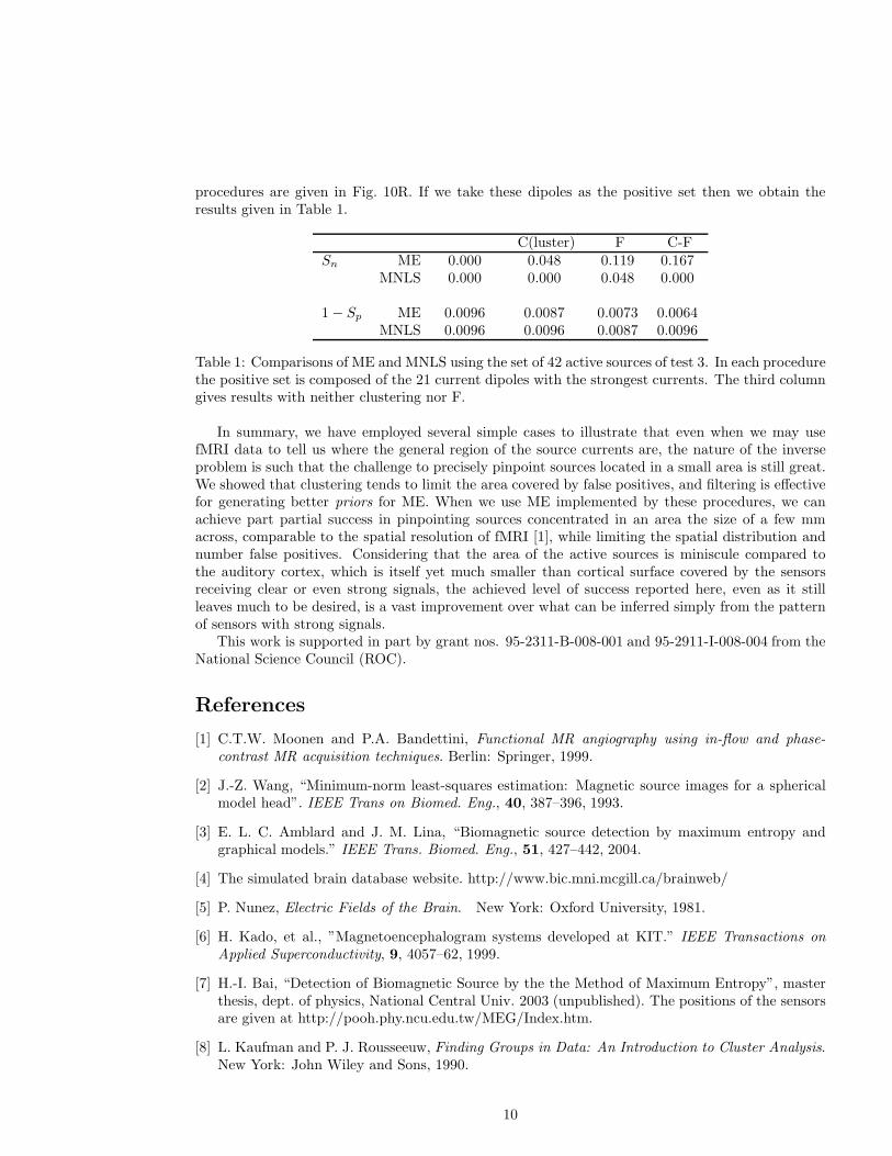
procedures are given in Fig. 10R. If we take these dipoles as the positive set then we obtain theresults given in Table 1.

C(luster) F C-FSn ME 0.000 0.048 0.119 0.167

MNLS 0.000 0.000 0.048 0.000

1 − Sp ME 0.0096 0.0087 0.0073 0.0064MNLS 0.0096 0.0096 0.0087 0.0096

Table 1: Comparisons of ME and MNLS using the set of 42 active sources of test 3. In each procedurethe positive set is composed of the 21 current dipoles with the strongest currents. The third columngives results with neither clustering nor F.

In summary, we have employed several simple cases to illustrate that even when we may usefMRI data to tell us where the general region of the source currents are, the nature of the inverseproblem is such that the challenge to precisely pinpoint sources located in a small area is still great.We showed that clustering tends to limit the area covered by false positives, and filtering is effectivefor generating better priors for ME. When we use ME implemented by these procedures, we canachieve part partial success in pinpointing sources concentrated in an area the size of a few mmacross, comparable to the spatial resolution of fMRI [1], while limiting the spatial distribution andnumber false positives. Considering that the area of the active sources is miniscule compared tothe auditory cortex, which is itself yet much smaller than cortical surface covered by the sensorsreceiving clear or even strong signals, the achieved level of success reported here, even as it stillleaves much to be desired, is a vast improvement over what can be inferred simply from the patternof sensors with strong signals.

This work is supported in part by grant nos. 95-2311-B-008-001 and 95-2911-I-008-004 from theNational Science Council (ROC).

References

[1] C.T.W. Moonen and P.A. Bandettini, Functional MR angiography using in-flow and phase-

contrast MR acquisition techniques. Berlin: Springer, 1999.

[2] J.-Z. Wang, “Minimum-norm least-squares estimation: Magnetic source images for a sphericalmodel head”. IEEE Trans on Biomed. Eng., 40, 387–396, 1993.

[3] E. L. C. Amblard and J. M. Lina, “Biomagnetic source detection by maximum entropy andgraphical models.” IEEE Trans. Biomed. Eng., 51, 427–442, 2004.

[4] The simulated brain database website. http://www.bic.mni.mcgill.ca/brainweb/

[5] P. Nunez, Electric Fields of the Brain. New York: Oxford University, 1981.

[6] H. Kado, et al., ”Magnetoencephalogram systems developed at KIT.” IEEE Transactions on

Applied Superconductivity, 9, 4057–62, 1999.

[7] H.-I. Bai, “Detection of Biomagnetic Source by the the Method of Maximum Entropy”, masterthesis, dept. of physics, National Central Univ. 2003 (unpublished). The positions of the sensorsare given at http://pooh.phy.ncu.edu.tw/MEG/Index.htm.

[8] L. Kaufman and P. J. Rousseeuw, Finding Groups in Data: An Introduction to Cluster Analysis.New York: John Wiley and Sons, 1990.

10

[9] T. Fawcett (2004), ”ROC Graphs: Notes and Practical Considerations for Researchers”, Tech-nical report, Palo Alto, USA: HP Laboratories.

[10] E. DeLong, D. DeLong and D. Clarke-Pearson, ”Comparing the areas under two or more cor-related receiver operating characteristic (ROC) curves: a nonparametric approach”, Biometrics,44, 837–845, 1988.

[11] C. J. S. Clarke and B. S. Janday, Inverse Problems, 5, 483–500, 1989; C. J. S. Clarke, ibid.

999–1012.

[12] L. K. Jones and V. Trutzer, “Computationally feasible high-resolution minimum-distance pro-cedures which extend the maximum- entropy method,” Inv. Prob., 5, 749-766, 1989.

[13] L. K. Jones and C. L. Byrne, “General entropy criteria for inverse problems, with applicationsto data compression, pattern classification, and cluster analysis,” IEEE Trans. Inform. Theory,36, 23-30, 1990.

[14] I. Csiszar, “Why least squares and maximum entropy? An axiomatic approach to inference forlinear inverse problems,” The Annals of Statistics, 19, 2032-2066, 1991.

[15] F. N. Alavi, J. G. Taylor and A. A. Ioannides, “Estimates of current density distributions: I.Applying the principle of cross-entropy minimization to electrographic recordings,” Inv. Prob.,9, 623–639, 1993.

[16] D. Khosla and M. Singh, “A maximum entropy method for MEG source imaging,” IEEE Trans.

Nuclear Sci., 44, 1368–1374, 1997.

[17] G. Le Besnerais, J.-F. Bercher and G. Demoment, “A new look at entropy for solving linearinverse problems,” IEEE Tran. Inf. Theory, 45, 1565–1578, 1999.

[18] R. He, L. Rao, S. Liu, W. Yan, P. A. Narayana and H. Brauer, “The method of maximummutual information for biomedical electromagnetic inverse problems,” IEEE Trans. Magnetics,36, 1741–1744, 2000.

[19] H. Gzyl, “Maximum entropy in the mean: A useful tool for constrained linear problems,” inBayesian Inference and Maximum Entropy in Science and Engineering, C. Williams, Ed. AIPConf. Proc. 659, Am. Inst. Phys., New York, 2002, pp.361-385.

[20] H.-I. Pai, C.-Y. Tseng, and H. C. Lee, “Identifying bio-magnetic sources by maximum entropyapproach”, in Bayesian Inference and Maximum entropy methods in Science and Engineering.Ed. K. Knuth, A. E. Abbas, R. D. Moris, and J. P. Castle, AIP Conf. Proc. 803, 527–534, 2005(copy available at http://xxx.lanl.gov/abs/qbio.NC/050804).

11