Data preprocessing

Data PreprocessingAdapted from:

Data Mining Concepts and Techniques by

Jiawei Han, Micheline Kamber and Jian Pei

Gajanand SharmaM E Scholar,UVCE Bangalore

Why preprocess the data?

Measuring the Central Tendency

Data cleaning

Data integration and transformation

Data reduction

Discretization and concept hierarchy generation

Content…

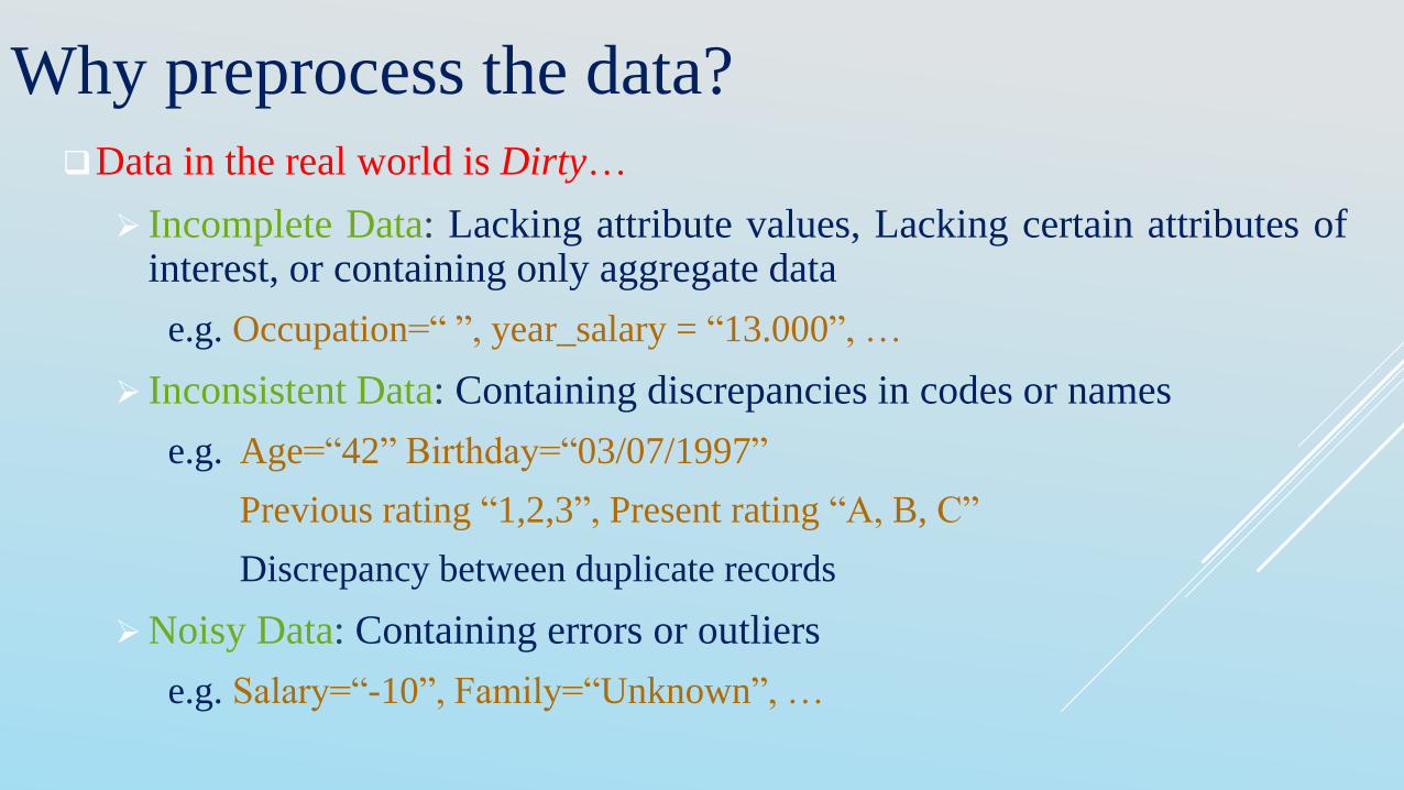
Data in the real world is Dirty…

Incomplete Data: Lacking attribute values, Lacking certain attributes ofinterest, or containing only aggregate data

e.g. Occupation=“ ”, year_salary = “13.000”, …

Inconsistent Data: Containing discrepancies in codes or names

e.g. Age=“42” Birthday=“03/07/1997”

Previous rating “1,2,3”, Present rating “A, B, C”

Discrepancy between duplicate records

Noisy Data: Containing errors or outliers

e.g. Salary=“-10”, Family=“Unknown”, …

Why preprocess the data?

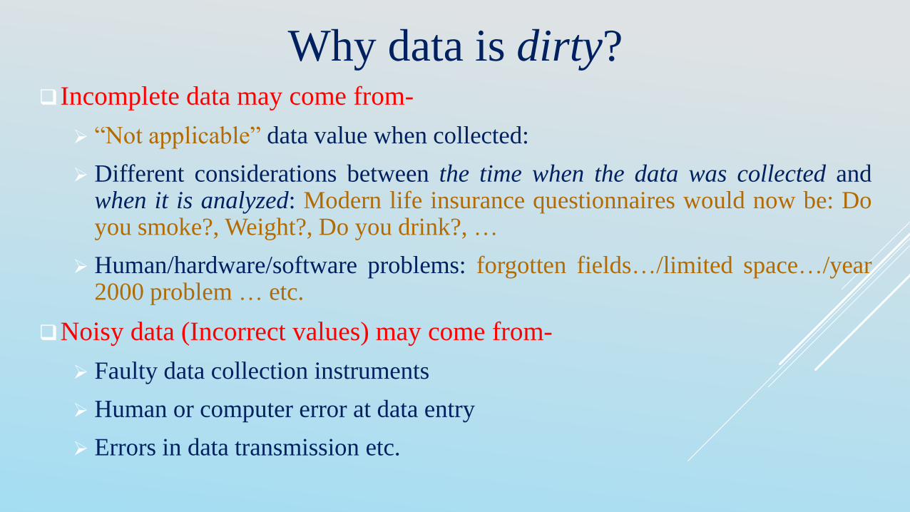
Why data is dirty?Incomplete data may come from-

“Not applicable” data value when collected:

Different considerations between the time when the data was collected andwhen it is analyzed: Modern life insurance questionnaires would now be: Doyou smoke?, Weight?, Do you drink?, …

Human/hardware/software problems: forgotten fields…/limited space…/year2000 problem … etc.

Noisy data (Incorrect values) may come from-

Faulty data collection instruments

Human or computer error at data entry

Errors in data transmission etc.

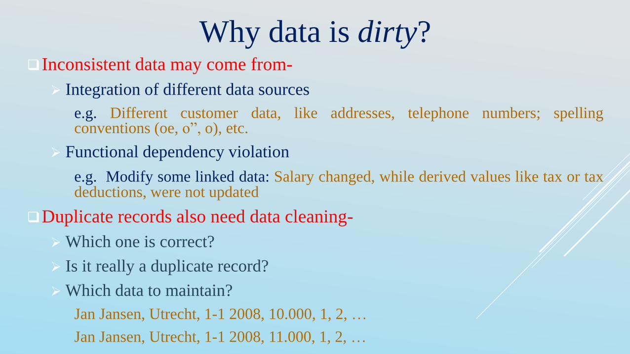
Why data is dirty?Inconsistent data may come from-

Integration of different data sources

e.g. Different customer data, like addresses, telephone numbers; spellingconventions (oe, o”, o), etc.

Functional dependency violation

e.g. Modify some linked data: Salary changed, while derived values like tax or taxdeductions, were not updated

Duplicate records also need data cleaning-

Which one is correct?

Is it really a duplicate record?

Which data to maintain?

Jan Jansen, Utrecht, 1-1 2008, 10.000, 1, 2, …

Jan Jansen, Utrecht, 1-1 2008, 11.000, 1, 2, …

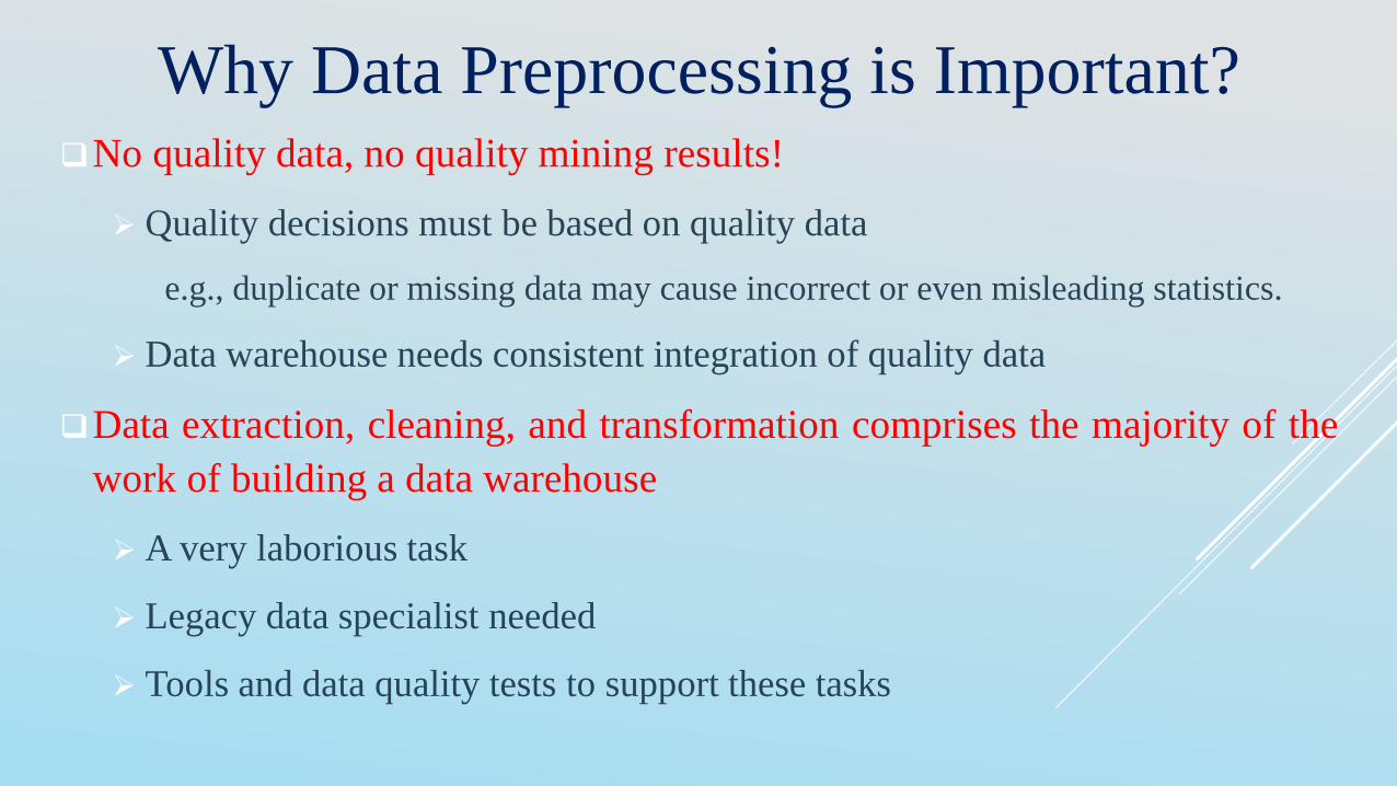
Why Data Preprocessing is Important?No quality data, no quality mining results!

Quality decisions must be based on quality data

e.g., duplicate or missing data may cause incorrect or even misleading statistics.

Data warehouse needs consistent integration of quality data

Data extraction, cleaning, and transformation comprises the majority of the

work of building a data warehouse

A very laborious task

Legacy data specialist needed

Tools and data quality tests to support these tasks

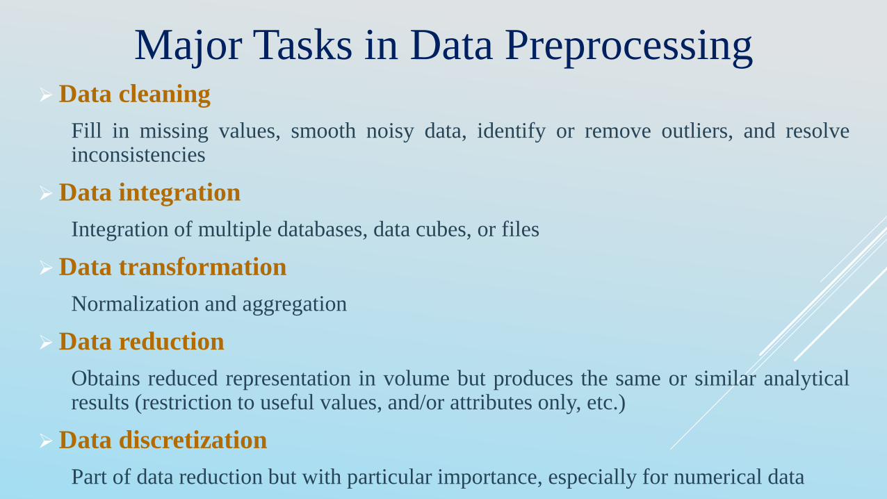
Major Tasks in Data PreprocessingData cleaning

Fill in missing values, smooth noisy data, identify or remove outliers, and resolveinconsistencies

Data integration

Integration of multiple databases, data cubes, or files

Data transformation

Normalization and aggregation

Data reduction

Obtains reduced representation in volume but produces the same or similar analyticalresults (restriction to useful values, and/or attributes only, etc.)

Data discretization

Part of data reduction but with particular importance, especially for numerical data

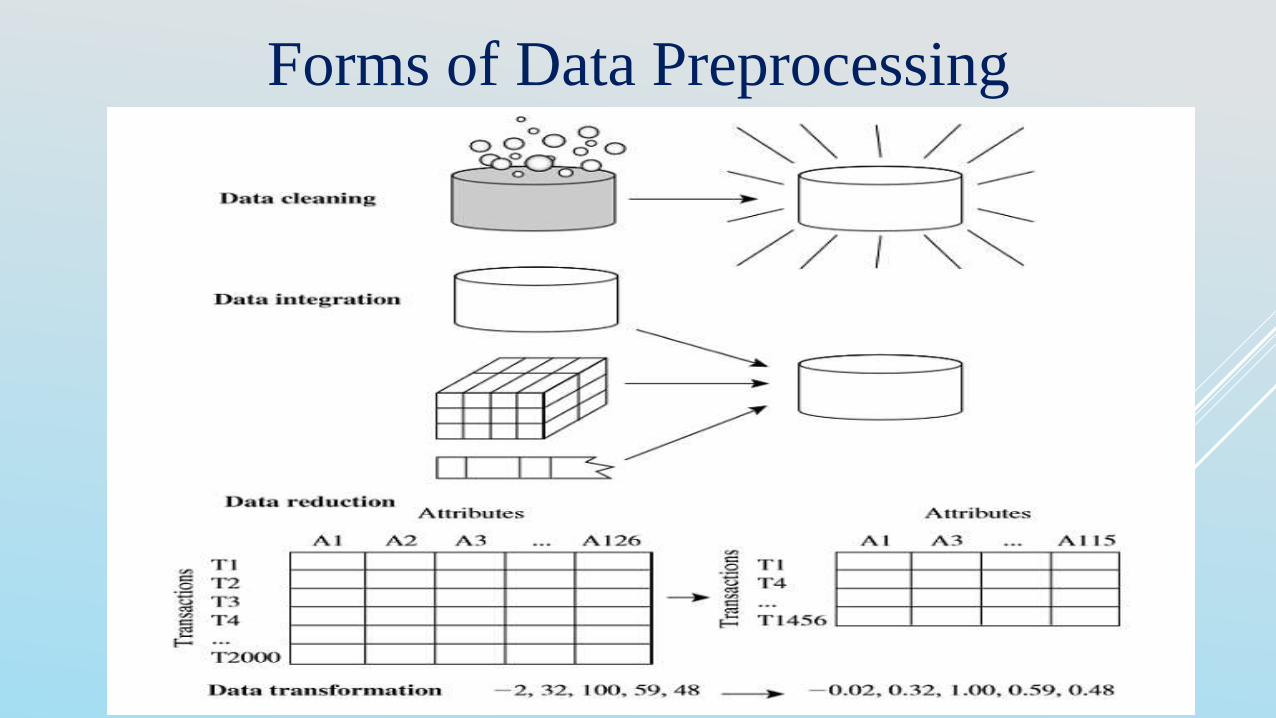
Forms of Data Preprocessing

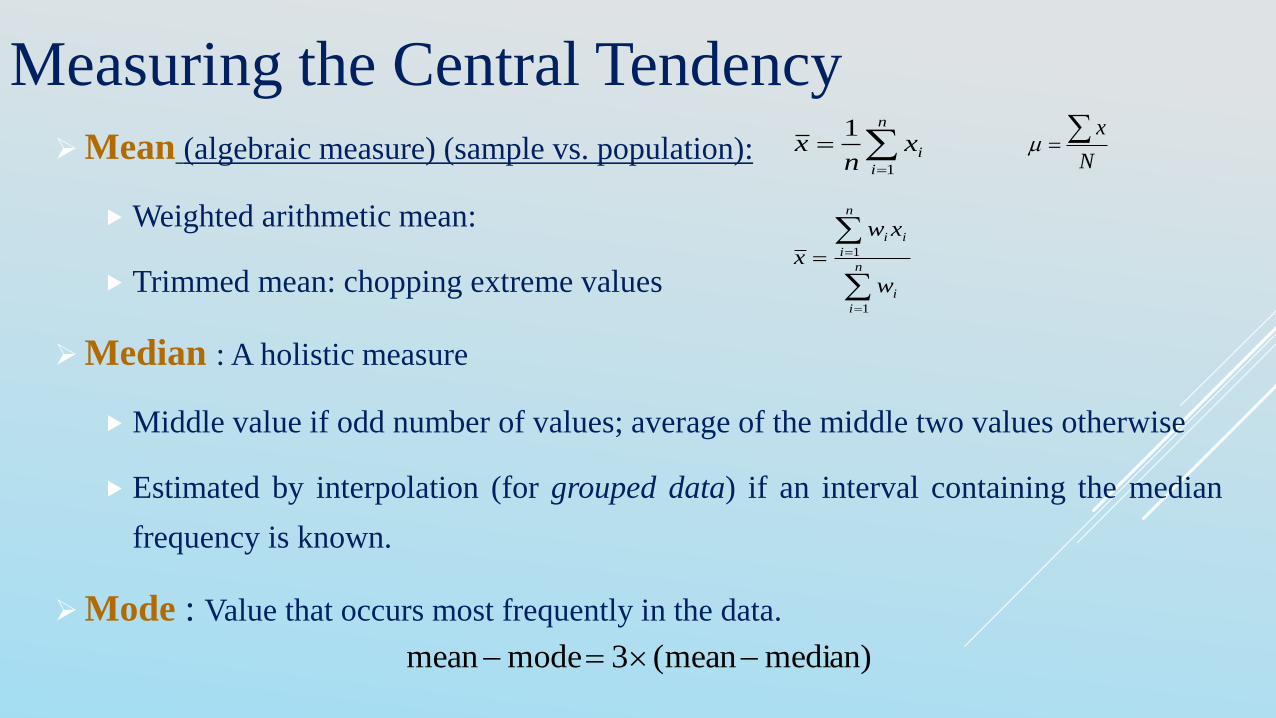
Measuring the Central Tendency

Mean (algebraic measure) (sample vs. population):

Weighted arithmetic mean:

Trimmed mean: chopping extreme values

Median : A holistic measure

Middle value if odd number of values; average of the middle two values otherwise

Estimated by interpolation (for grouped data) if an interval containing the median

frequency is known.

Mode : Value that occurs most frequently in the data.

n

i

ixn

x1

1

N

x

n

i

i

n

i

ii

w

xw

x

1

1

median)(mean3modemean

Data CleaningWhy Data Cleaning?

“Data cleaning is one of the three biggest problems in data warehousing”—RalphKimball

“Data cleaning is the number one problem in data warehousing”—DCI survey

Data cleaning tasks

Fill in missing values

Identify outliers and smooth out noisy data

Correct inconsistent data

Resolve redundancy caused by data integration

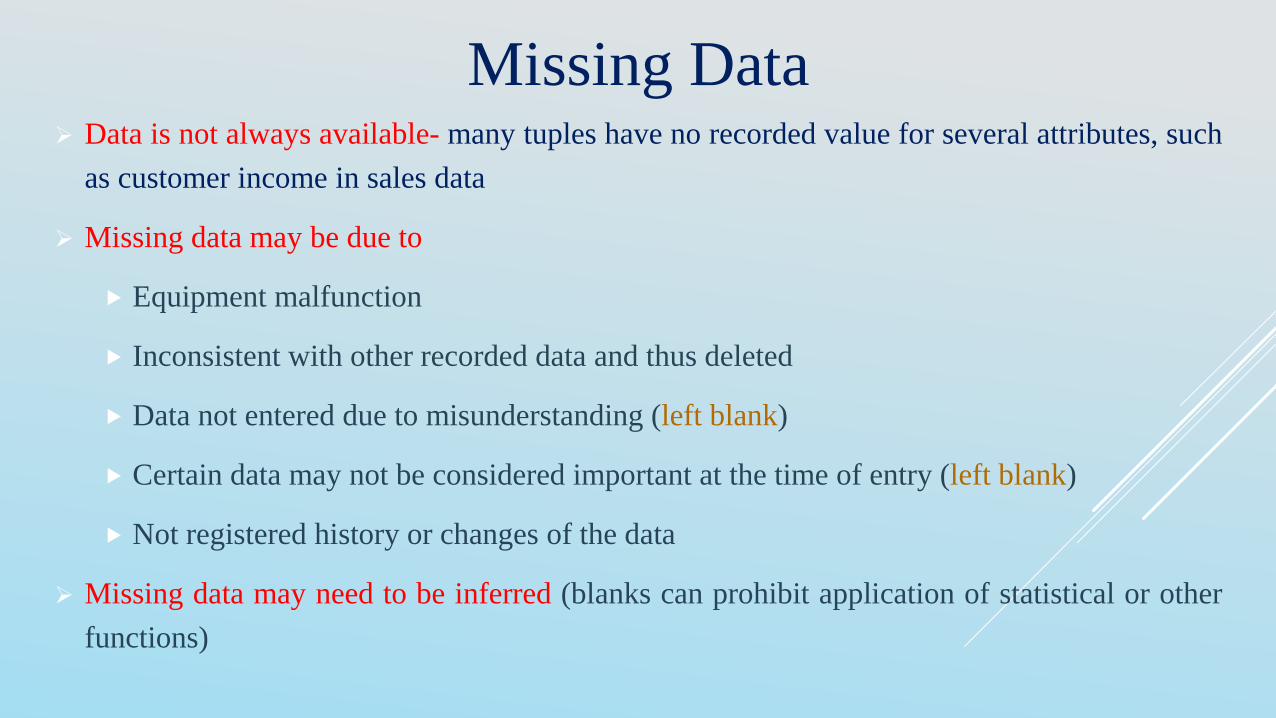
Missing Data Data is not always available- many tuples have no recorded value for several attributes, such

as customer income in sales data

Missing data may be due to

Equipment malfunction

Inconsistent with other recorded data and thus deleted

Data not entered due to misunderstanding (left blank)

Certain data may not be considered important at the time of entry (left blank)

Not registered history or changes of the data

Missing data may need to be inferred (blanks can prohibit application of statistical or other

functions)

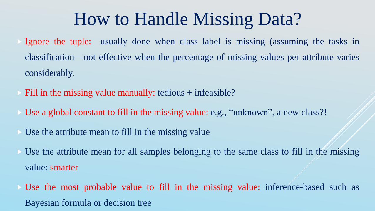
How to Handle Missing Data? Ignore the tuple: usually done when class label is missing (assuming the tasks in

classification—not effective when the percentage of missing values per attribute varies

considerably.

Fill in the missing value manually: tedious + infeasible?

Use a global constant to fill in the missing value: e.g., “unknown”, a new class?!

Use the attribute mean to fill in the missing value

Use the attribute mean for all samples belonging to the same class to fill in the missing

value: smarter

Use the most probable value to fill in the missing value: inference-based such as

Bayesian formula or decision tree

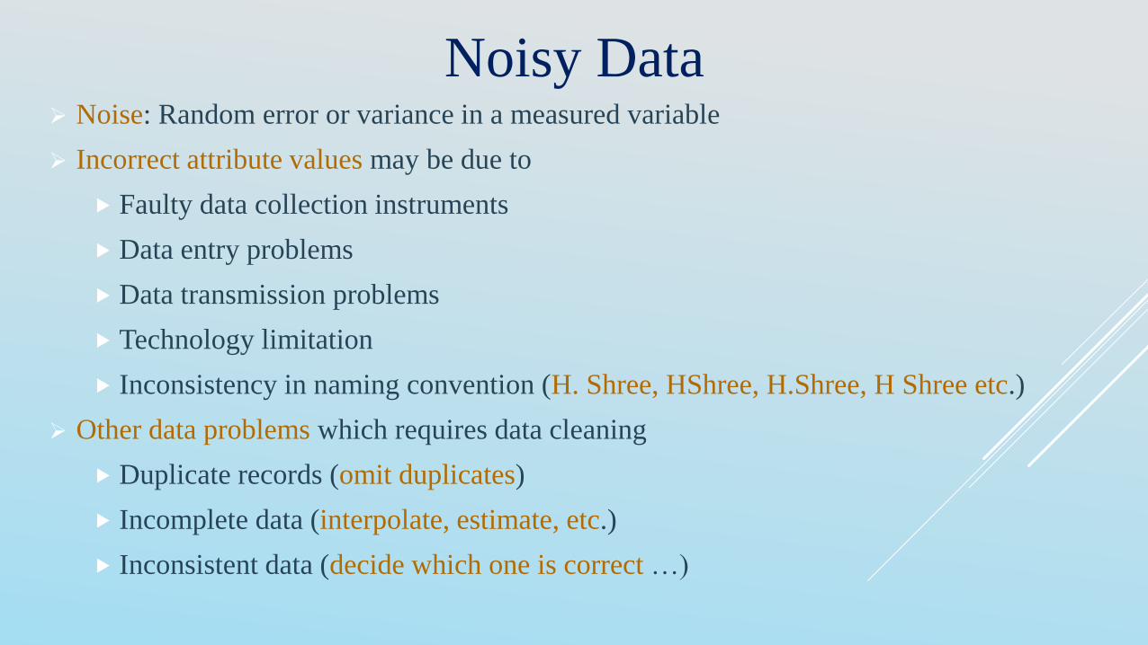
Noisy Data Noise: Random error or variance in a measured variable

Incorrect attribute values may be due to

Faulty data collection instruments

Data entry problems

Data transmission problems

Technology limitation

Inconsistency in naming convention (H. Shree, HShree, H.Shree, H Shree etc.)

Other data problems which requires data cleaning

Duplicate records (omit duplicates)

Incomplete data (interpolate, estimate, etc.)

Inconsistent data (decide which one is correct …)

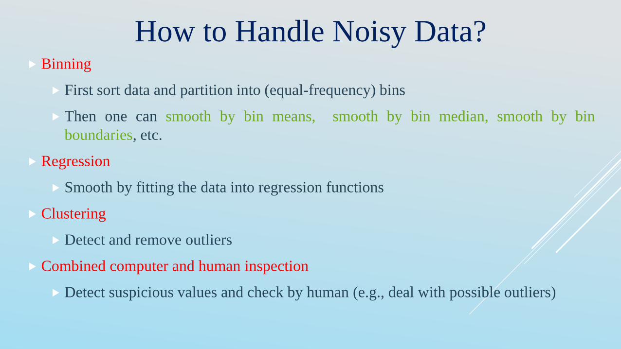
How to Handle Noisy Data? Binning

First sort data and partition into (equal-frequency) bins

Then one can smooth by bin means, smooth by bin median, smooth by bin

boundaries, etc.

Regression

Smooth by fitting the data into regression functions

Clustering

Detect and remove outliers

Combined computer and human inspection

Detect suspicious values and check by human (e.g., deal with possible outliers)

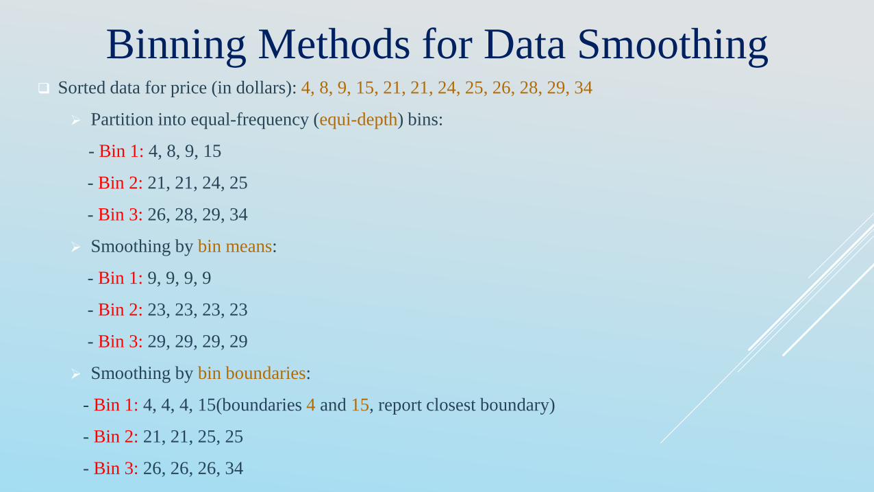
Binning Methods for Data Smoothing Sorted data for price (in dollars): 4, 8, 9, 15, 21, 21, 24, 25, 26, 28, 29, 34

Partition into equal-frequency (equi-depth) bins:

- Bin 1: 4, 8, 9, 15

- Bin 2: 21, 21, 24, 25

- Bin 3: 26, 28, 29, 34

Smoothing by bin means:

- Bin 1: 9, 9, 9, 9

- Bin 2: 23, 23, 23, 23

- Bin 3: 29, 29, 29, 29

Smoothing by bin boundaries:

- Bin 1: 4, 4, 4, 15(boundaries 4 and 15, report closest boundary)

- Bin 2: 21, 21, 25, 25

- Bin 3: 26, 26, 26, 34

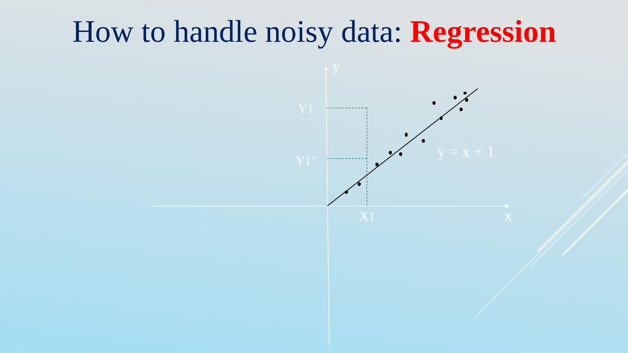
How to handle noisy data: Regression

y = x + 1

x

y

Y1

Y1’

X1

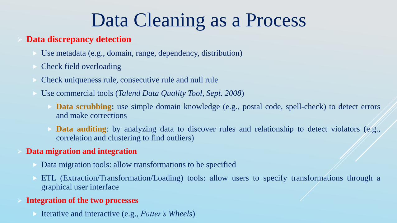
Data Cleaning as a Process Data discrepancy detection

Use metadata (e.g., domain, range, dependency, distribution)

Check field overloading

Check uniqueness rule, consecutive rule and null rule

Use commercial tools (Talend Data Quality Tool, Sept. 2008)

Data scrubbing: use simple domain knowledge (e.g., postal code, spell-check) to detect errorsand make corrections

Data auditing: by analyzing data to discover rules and relationship to detect violators (e.g.,correlation and clustering to find outliers)

Data migration and integration

Data migration tools: allow transformations to be specified

ETL (Extraction/Transformation/Loading) tools: allow users to specify transformations through agraphical user interface

Integration of the two processes

Iterative and interactive (e.g., Potter’s Wheels)

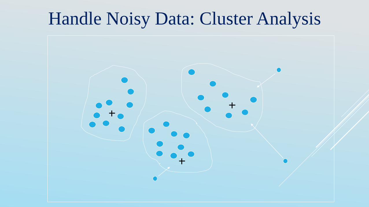
Handle Noisy Data: Cluster Analysis

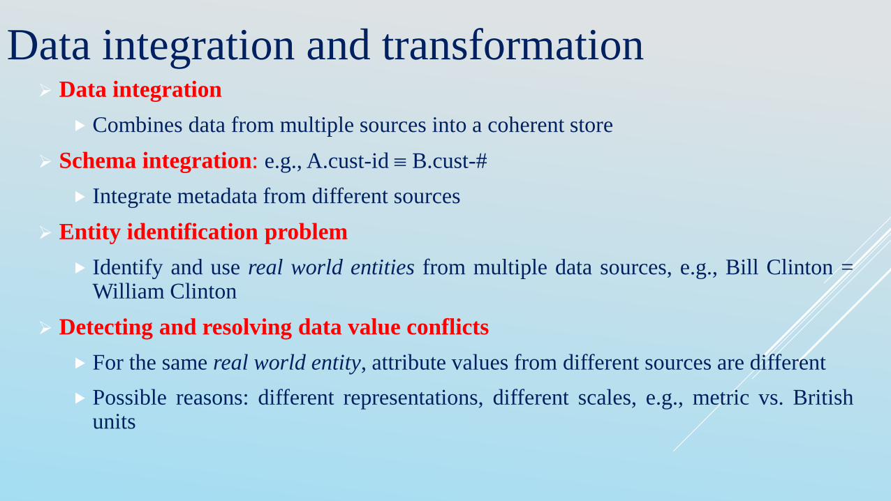
Data integration

Combines data from multiple sources into a coherent store

Schema integration: e.g., A.cust-id B.cust-#

Integrate metadata from different sources

Entity identification problem

Identify and use real world entities from multiple data sources, e.g., Bill Clinton =William Clinton

Detecting and resolving data value conflicts

For the same real world entity, attribute values from different sources are different

Possible reasons: different representations, different scales, e.g., metric vs. Britishunits

Data integration and transformation

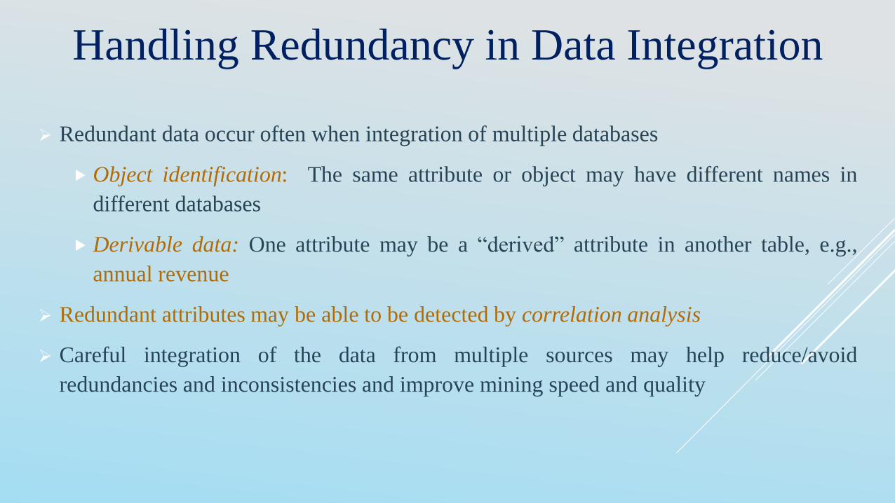
Redundant data occur often when integration of multiple databases

Object identification: The same attribute or object may have different names in

different databases

Derivable data: One attribute may be a “derived” attribute in another table, e.g.,

annual revenue

Redundant attributes may be able to be detected by correlation analysis

Careful integration of the data from multiple sources may help reduce/avoid

redundancies and inconsistencies and improve mining speed and quality

Handling Redundancy in Data Integration

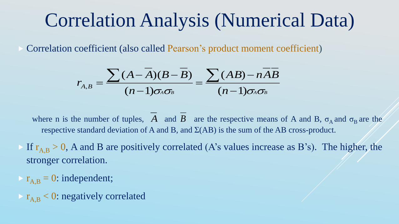
Correlation coefficient (also called Pearson’s product moment coefficient)

where n is the number of tuples, and are the respective means of A and B, σA and σB are the

respective standard deviation of A and B, and Σ(AB) is the sum of the AB cross-product.

If rA,B > 0, A and B are positively correlated (A’s values increase as B’s). The higher, the

stronger correlation.

rA,B = 0: independent;

rA,B < 0: negatively correlated

Correlation Analysis (Numerical Data)

BABA n

BAnAB

n

BBAAr BA

)1(

)(

)1(

))((,

A B

Correlation Analysis (Categorial Data)

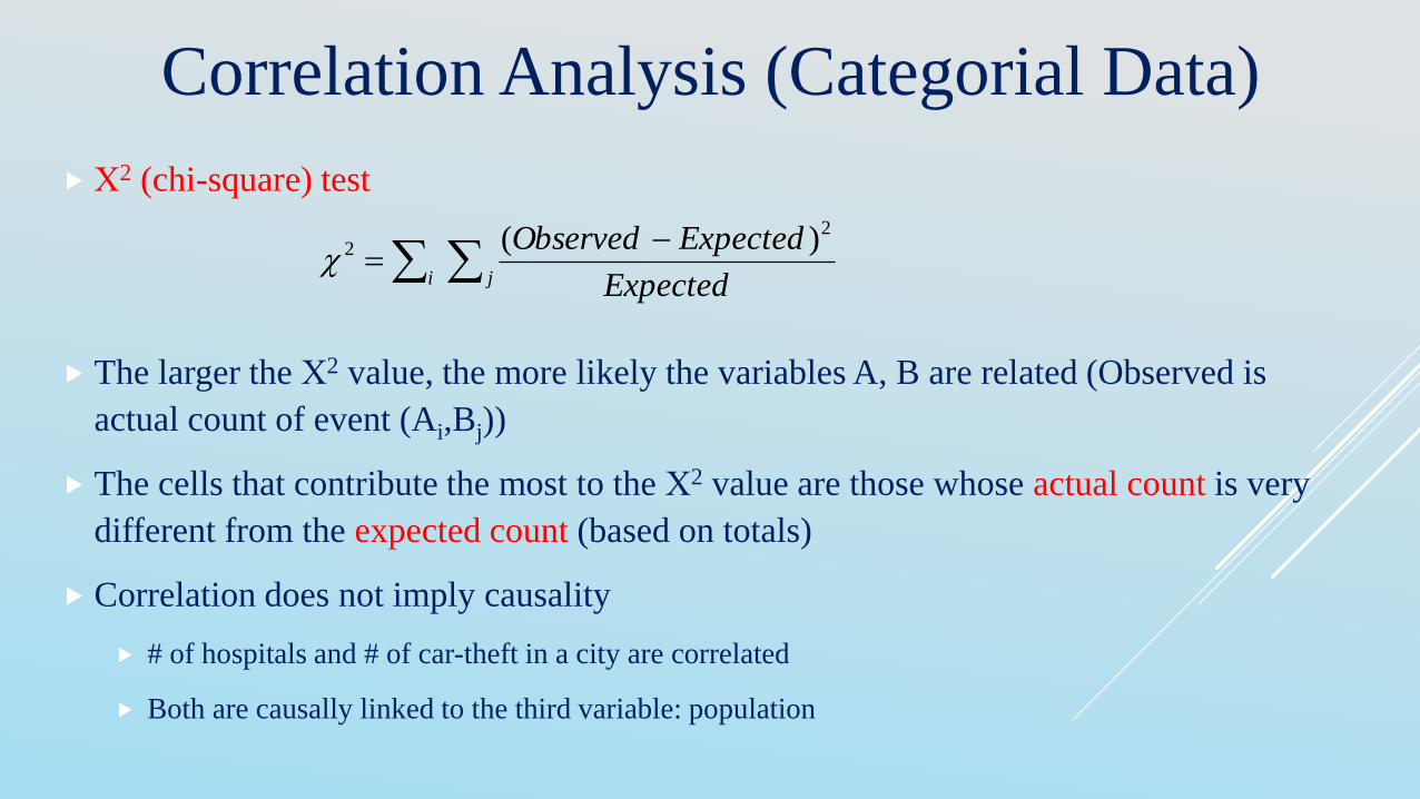
Χ2 (chi-square) test

The larger the Χ2 value, the more likely the variables A, B are related (Observed is

actual count of event (Ai,Bj))

The cells that contribute the most to the Χ2 value are those whose actual count is very

different from the expected count (based on totals)

Correlation does not imply causality

# of hospitals and # of car-theft in a city are correlated

Both are causally linked to the third variable: population

ji Expected

ExpectedObserved 22 )(

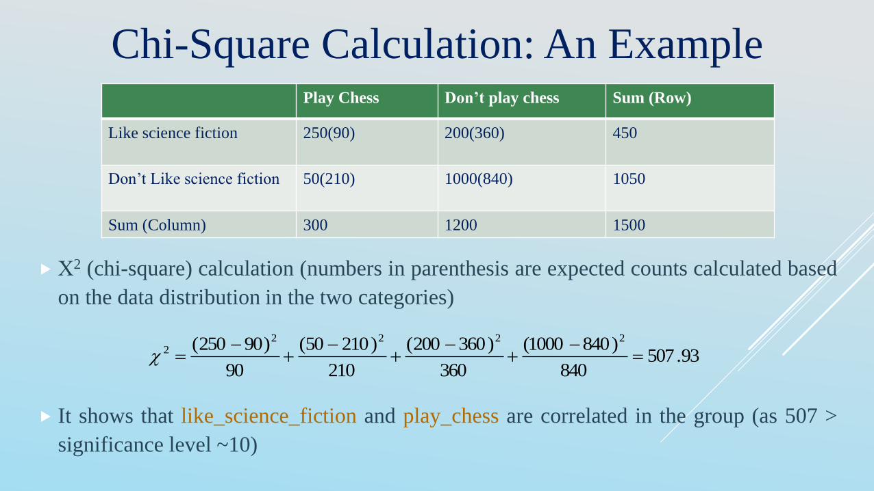
Chi-Square Calculation: An Example

Χ2 (chi-square) calculation (numbers in parenthesis are expected counts calculated based

on the data distribution in the two categories)

It shows that like_science_fiction and play_chess are correlated in the group (as 507 >

significance level ~10)

93.507840

)8401000(

360

)360200(

210

)21050(

90

)90250( 22222

Play Chess Don’t play chess Sum (Row)

Like science fiction 250(90) 200(360) 450

Don’t Like science fiction 50(210) 1000(840) 1050

Sum (Column) 300 1200 1500

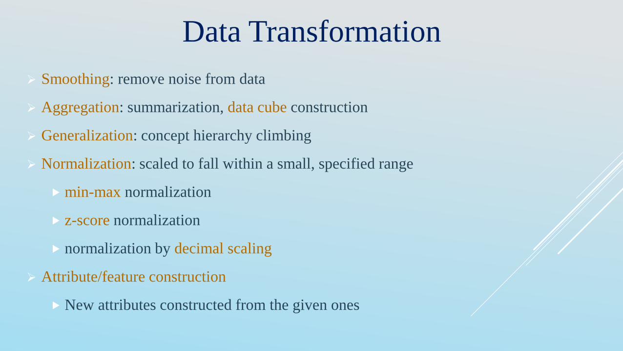
Data Transformation

Smoothing: remove noise from data

Aggregation: summarization, data cube construction

Generalization: concept hierarchy climbing

Normalization: scaled to fall within a small, specified range

min-max normalization

z-score normalization

normalization by decimal scaling

Attribute/feature construction

New attributes constructed from the given ones

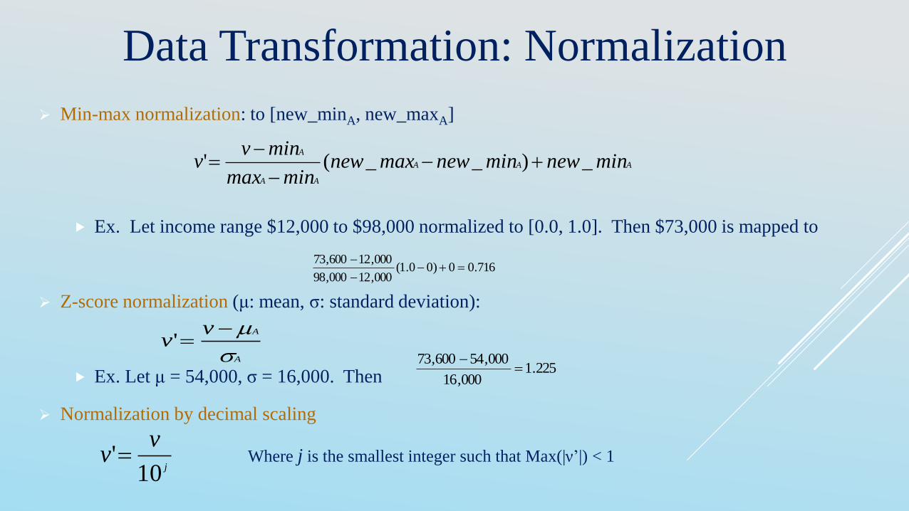
Data Transformation: Normalization

Min-max normalization: to [new_minA, new_maxA]

Ex. Let income range $12,000 to $98,000 normalized to [0.0, 1.0]. Then $73,000 is mapped to

Z-score normalization (μ: mean, σ: standard deviation):

Ex. Let μ = 54,000, σ = 16,000. Then

Normalization by decimal scaling

AAA

AA

A

minnewminnewmaxnewminmax

minvv _)__('

716.00)00.1(000,12000,98

000,12600,73

A

Avv

'

225.1000,16

000,54600,73

j

vv

10' Where j is the smallest integer such that Max(|ν’|) < 1

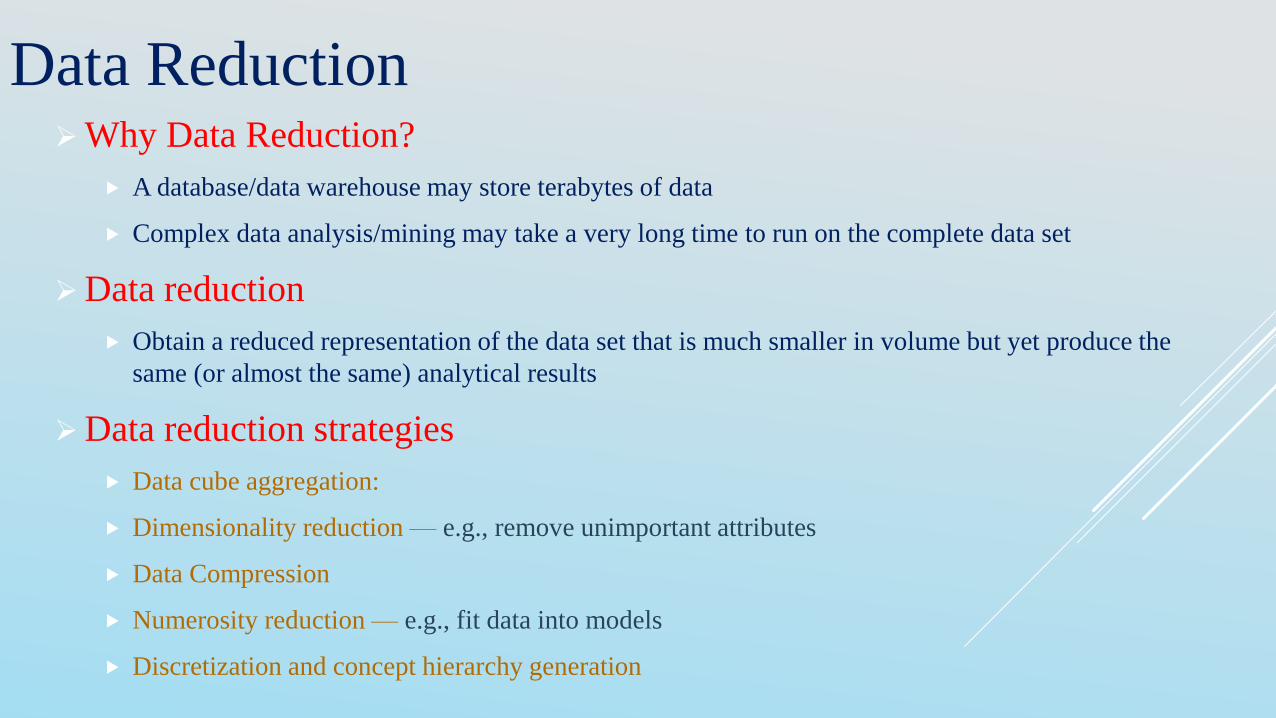
Data ReductionWhy Data Reduction?

A database/data warehouse may store terabytes of data

Complex data analysis/mining may take a very long time to run on the complete data set

Data reduction

Obtain a reduced representation of the data set that is much smaller in volume but yet produce the

same (or almost the same) analytical results

Data reduction strategies

Data cube aggregation:

Dimensionality reduction — e.g., remove unimportant attributes

Data Compression

Numerosity reduction — e.g., fit data into models

Discretization and concept hierarchy generation

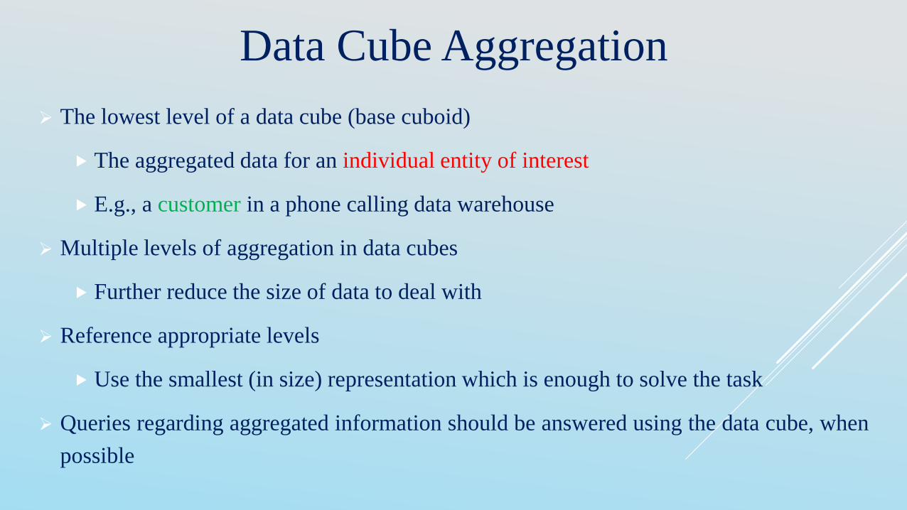
Data Cube Aggregation

The lowest level of a data cube (base cuboid)

The aggregated data for an individual entity of interest

E.g., a customer in a phone calling data warehouse

Multiple levels of aggregation in data cubes

Further reduce the size of data to deal with

Reference appropriate levels

Use the smallest (in size) representation which is enough to solve the task

Queries regarding aggregated information should be answered using the data cube, when

possible

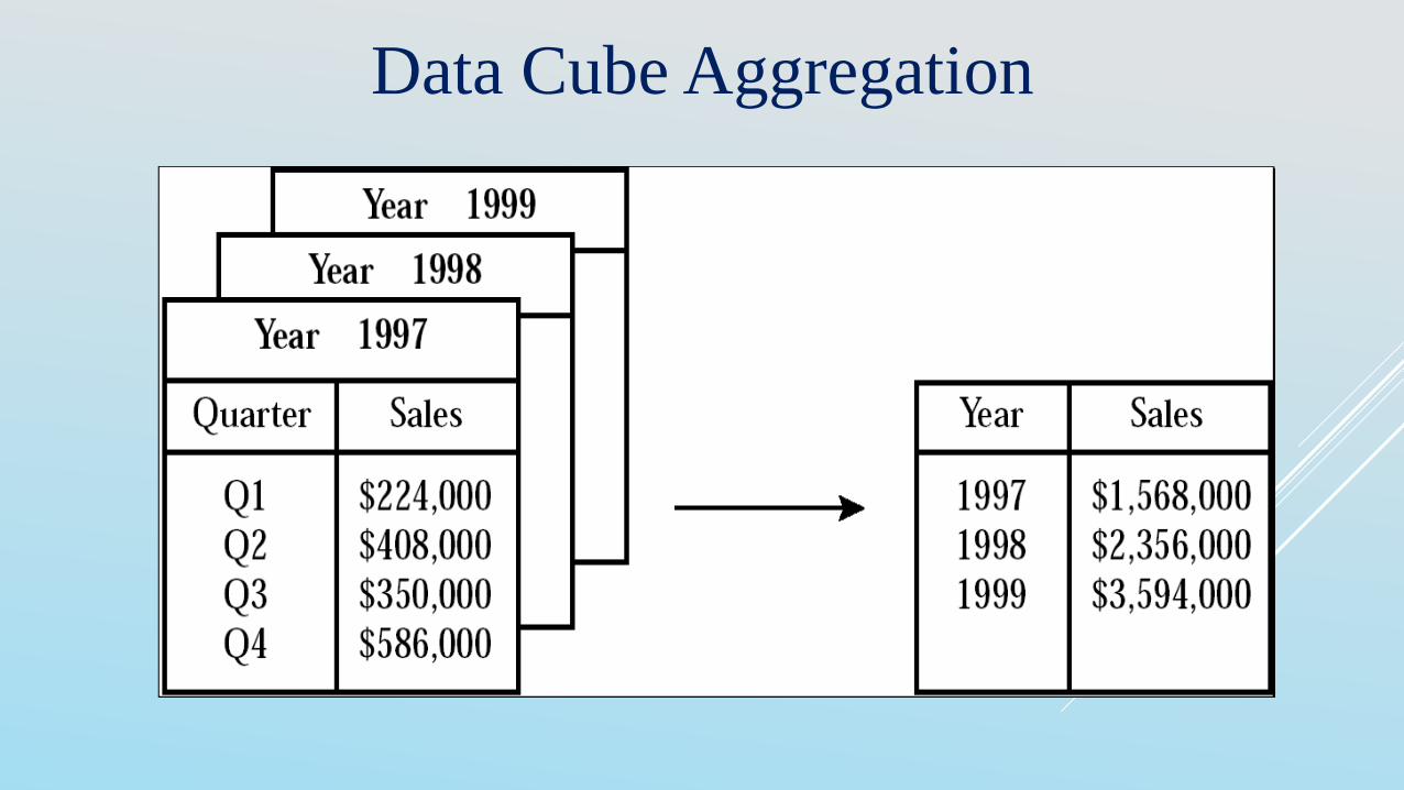
Data Cube Aggregation

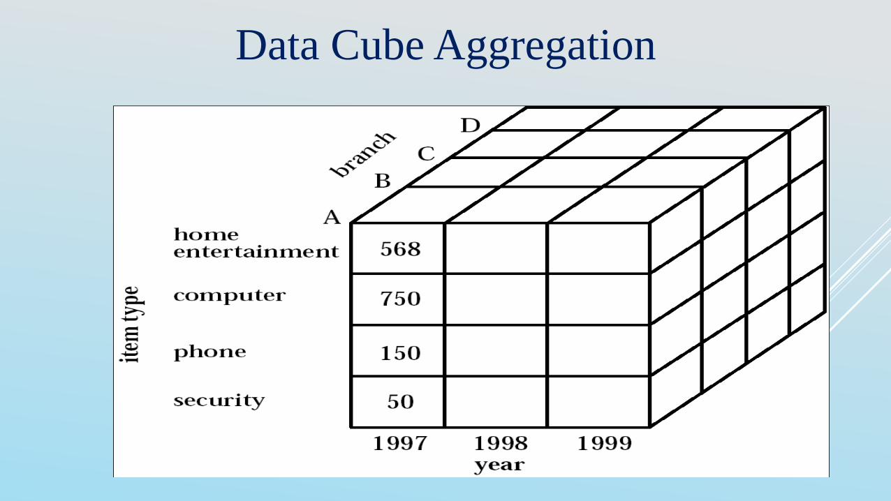
Data Cube Aggregation

Attribute Subset Selection

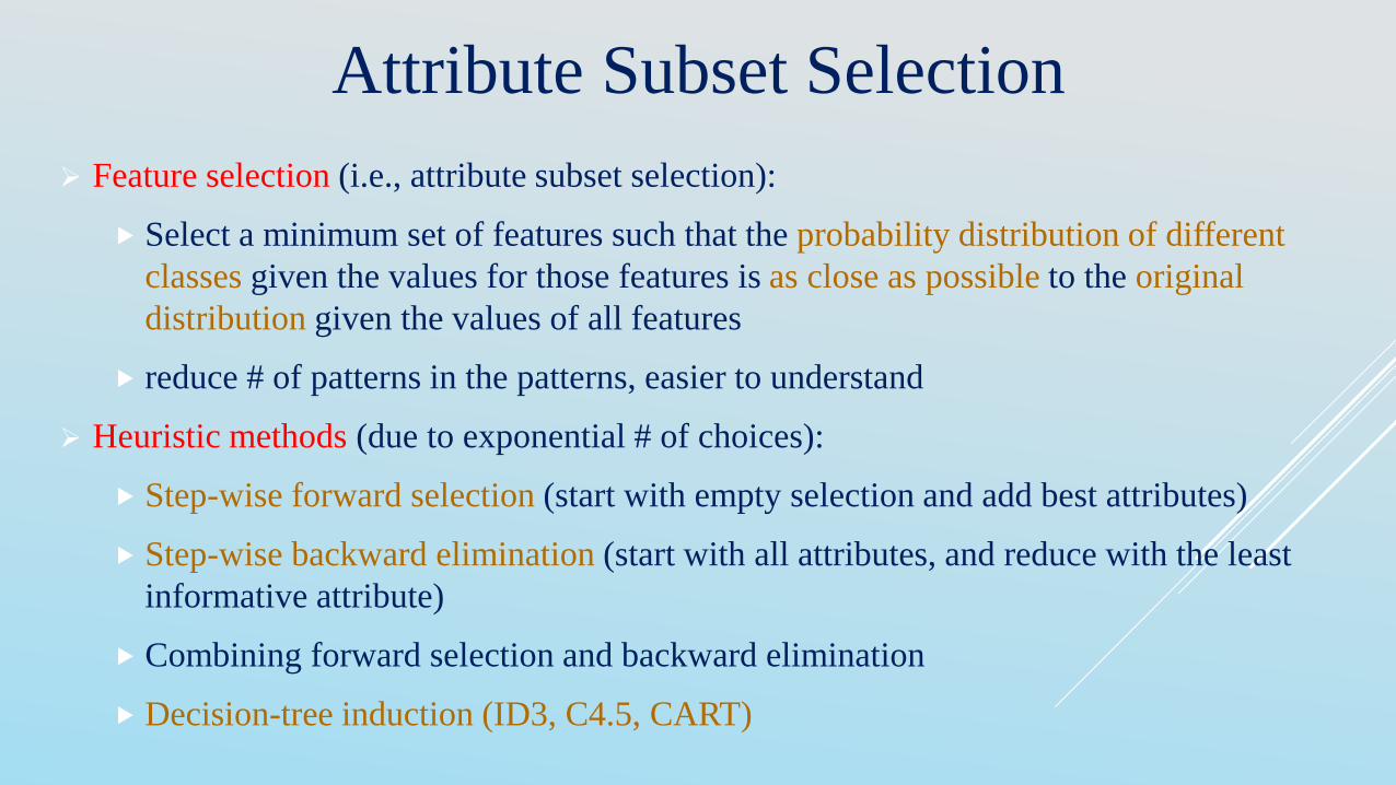
Feature selection (i.e., attribute subset selection):

Select a minimum set of features such that the probability distribution of different

classes given the values for those features is as close as possible to the original

distribution given the values of all features

reduce # of patterns in the patterns, easier to understand

Heuristic methods (due to exponential # of choices):

Step-wise forward selection (start with empty selection and add best attributes)

Step-wise backward elimination (start with all attributes, and reduce with the least

informative attribute)

Combining forward selection and backward elimination

Decision-tree induction (ID3, C4.5, CART)

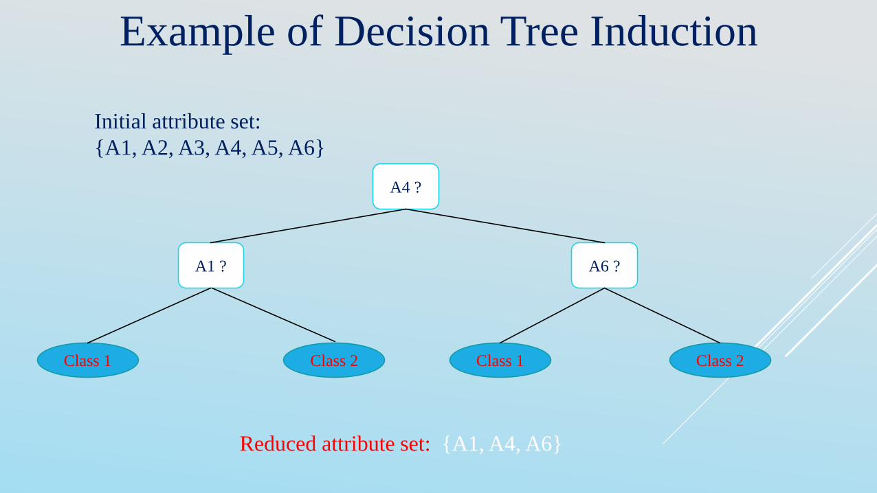
Example of Decision Tree Induction

Initial attribute set:

{A1, A2, A3, A4, A5, A6}

Class 2Class 1Class 1 Class 2

A4 ?

A6 ?A1 ?

Reduced attribute set: {A1, A4, A6}

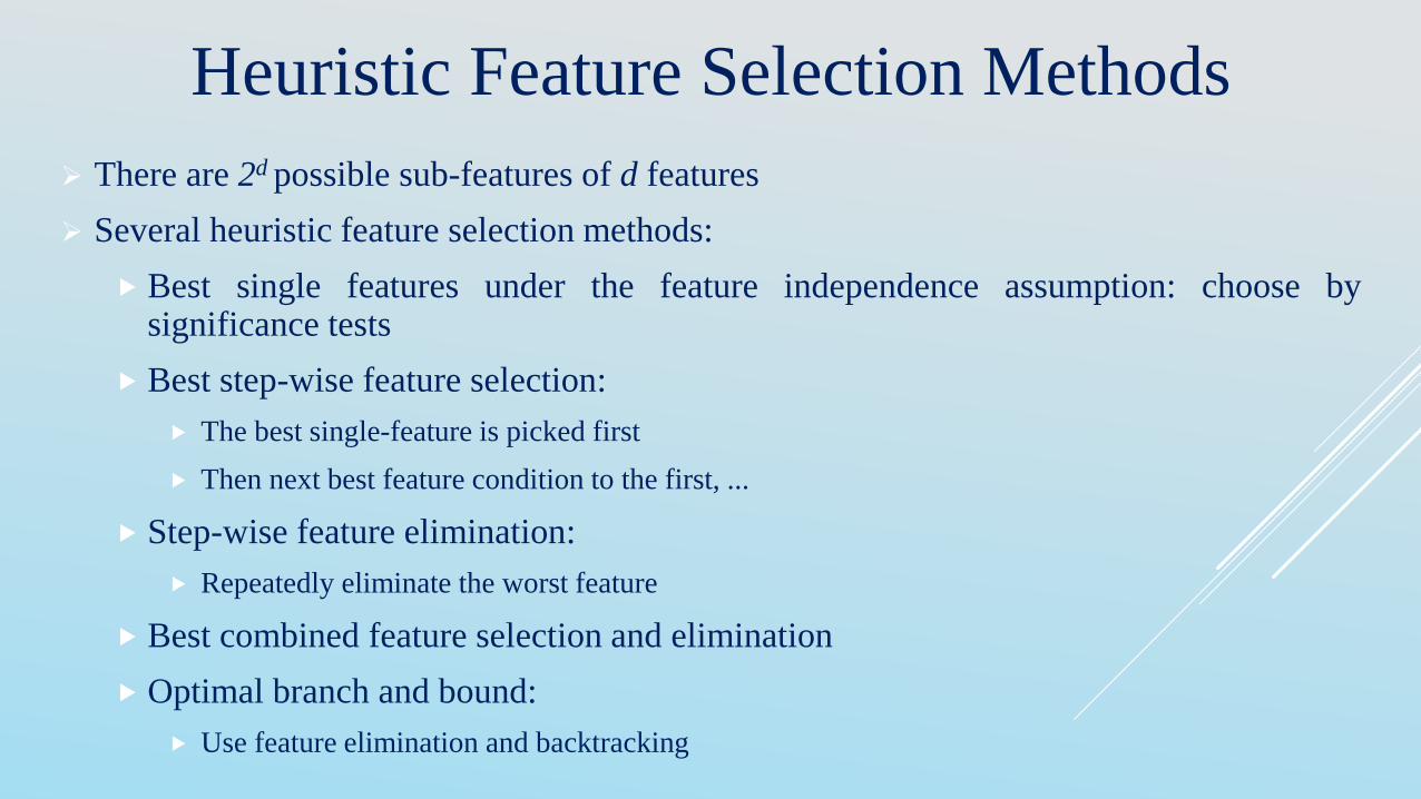
Heuristic Feature Selection Methods

There are 2d possible sub-features of d features

Several heuristic feature selection methods:

Best single features under the feature independence assumption: choose bysignificance tests

Best step-wise feature selection:

The best single-feature is picked first

Then next best feature condition to the first, ...

Step-wise feature elimination:

Repeatedly eliminate the worst feature

Best combined feature selection and elimination

Optimal branch and bound:

Use feature elimination and backtracking

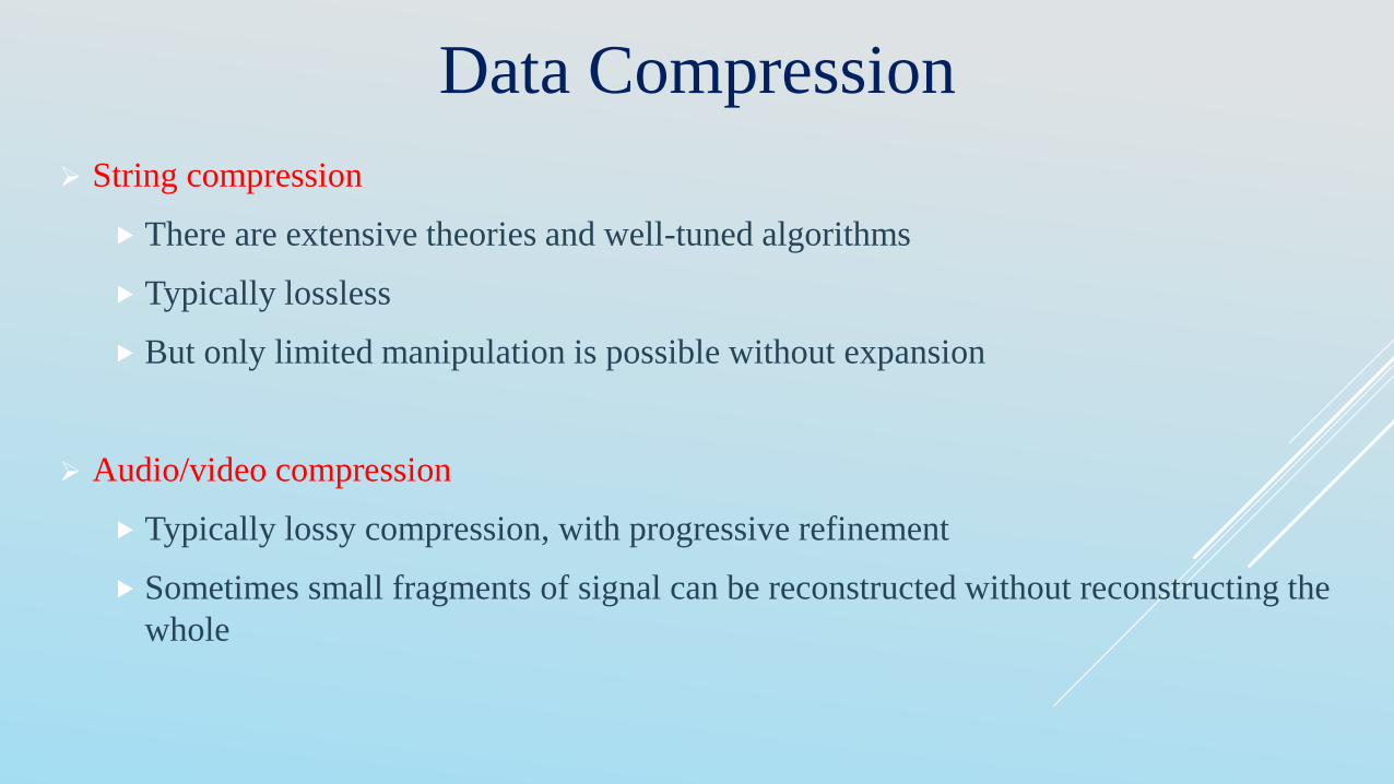
Data Compression

String compression

There are extensive theories and well-tuned algorithms

Typically lossless

But only limited manipulation is possible without expansion

Audio/video compression

Typically lossy compression, with progressive refinement

Sometimes small fragments of signal can be reconstructed without reconstructing the

whole

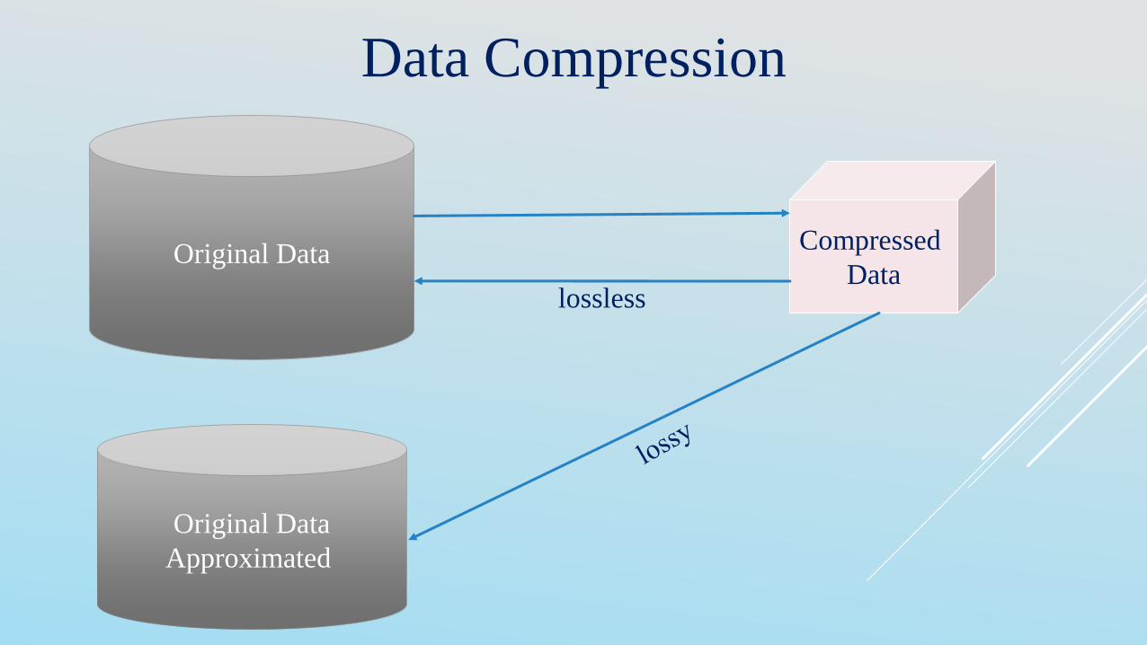
Data Compression

Original Data

Original Data

Approximated

Compressed

Datalossless

Regression

Predict a value of a given continuous valued variable based on thevalues of other variables, assuming a linear or nonlinear model ofdependency.

Greatly studied in statistics, neural network fields.

Examples:

Predicting sales amounts of new product based on advertisingexpenditure.

Predicting wind velocities as a function of temperature, humidity, airpressure, etc.

Time series prediction of stock market indices.

Data Reduction Method (1): Regression

Linear regression: Data are modeled to fit a straight line

Often uses the least-square method to fit the line

Y = w X + b

Two regression coefficients, w and b, specify the line and are to be estimated by using the

data at hand

Using the least squares criterion to the known values of Y1, Y2, …, X1, X2, ….

Multiple regression: Allows a response variable Y to be modeled as a linear function of a

multidimensional feature vector

Y = b0 + b1 X1 + b2 X2.

Many nonlinear functions can be transformed into the above

Data Reduction Method (2): Histograms

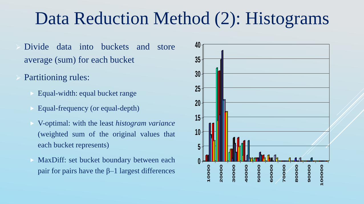
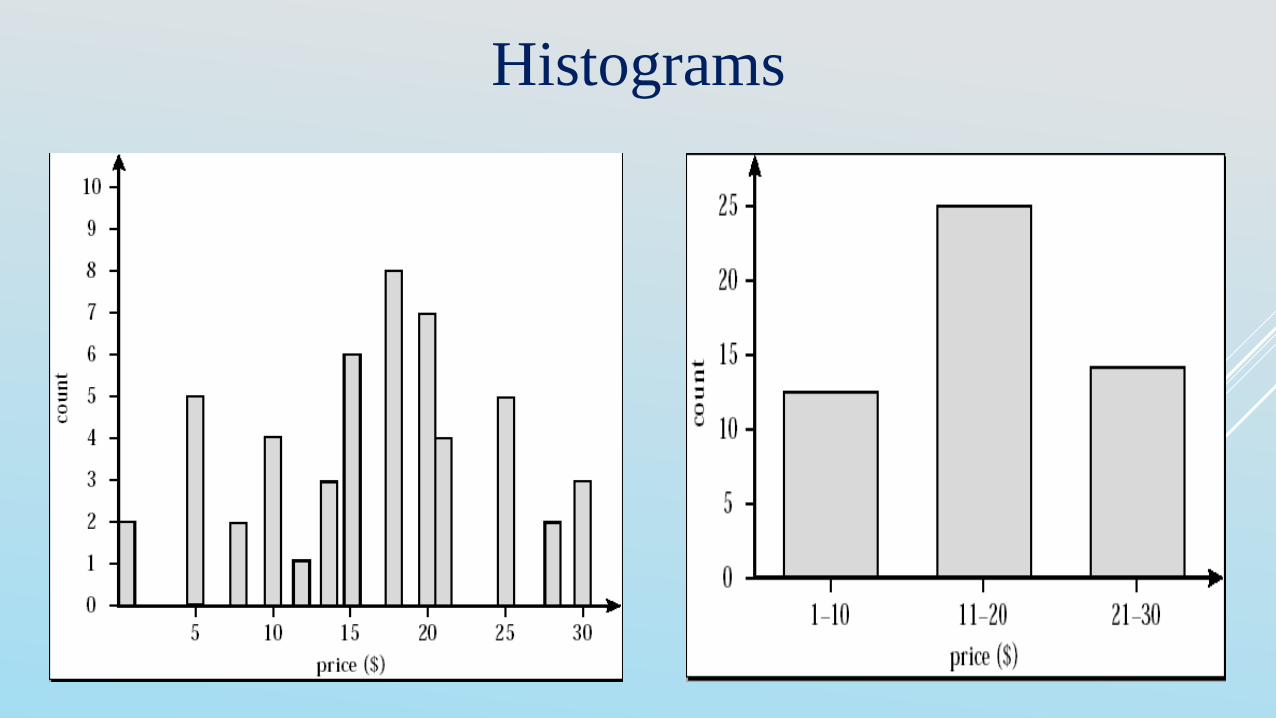
Divide data into buckets and store

average (sum) for each bucket

Partitioning rules:

Equal-width: equal bucket range

Equal-frequency (or equal-depth)

V-optimal: with the least histogram variance

(weighted sum of the original values that

each bucket represents)

MaxDiff: set bucket boundary between each

pair for pairs have the β–1 largest differences

0

5

10

15

20

25

30

35

40

10

00

0

20

00

0

30

00

0

40

00

0

50

00

0

60

00

0

70

00

0

80

00

0

90

00

0

10

00

00

Histograms

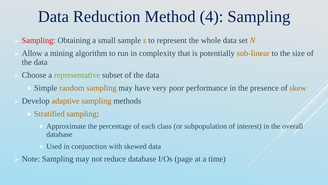
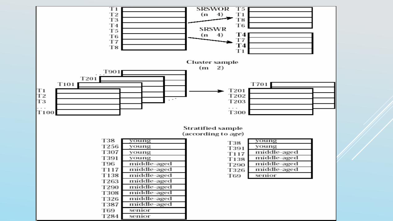
Data Reduction Method (4): Sampling

Sampling: Obtaining a small sample s to represent the whole data set N

Allow a mining algorithm to run in complexity that is potentially sub-linear to the size of the data

Choose a representative subset of the data

Simple random sampling may have very poor performance in the presence of skew

Develop adaptive sampling methods

Stratified sampling:

Approximate the percentage of each class (or subpopulation of interest) in the overall database

Used in conjunction with skewed data

Note: Sampling may not reduce database I/Os (page at a time)

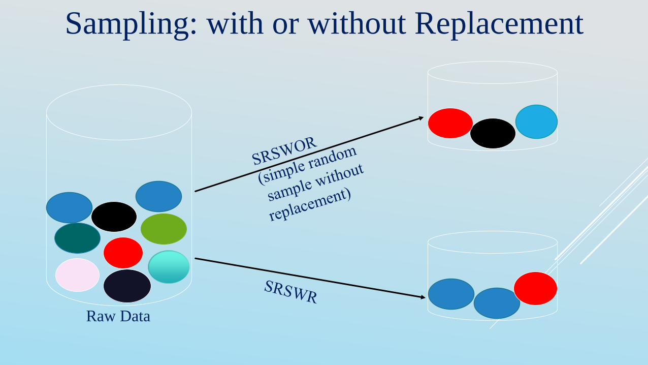
Sampling: with or without Replacement

Raw Data

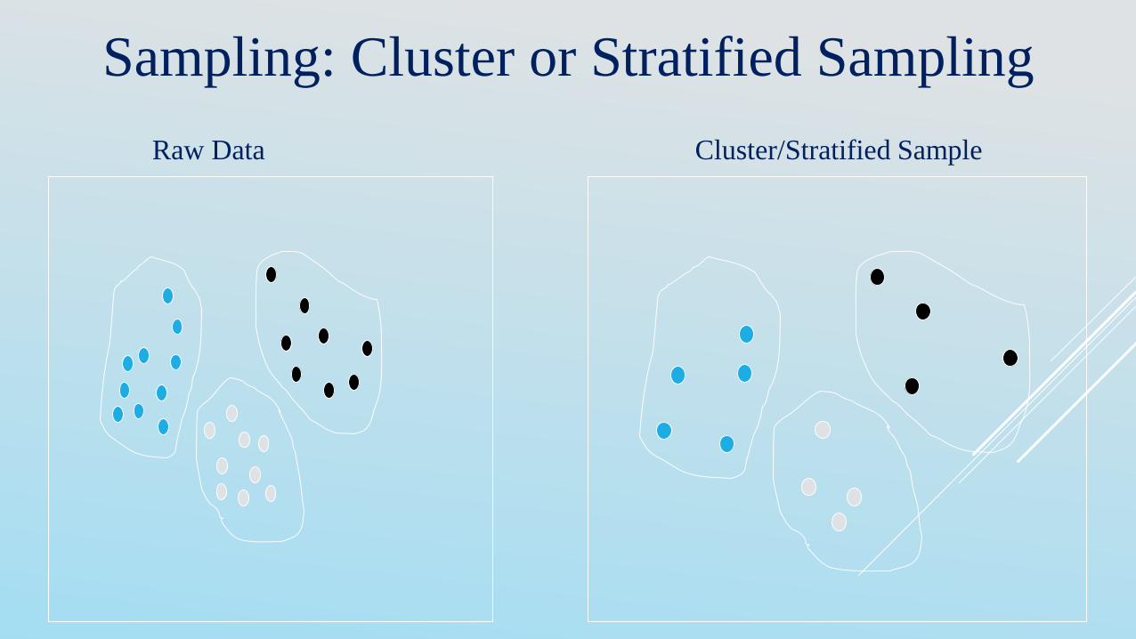
Sampling: Cluster or Stratified Sampling

Raw Data Cluster/Stratified Sample

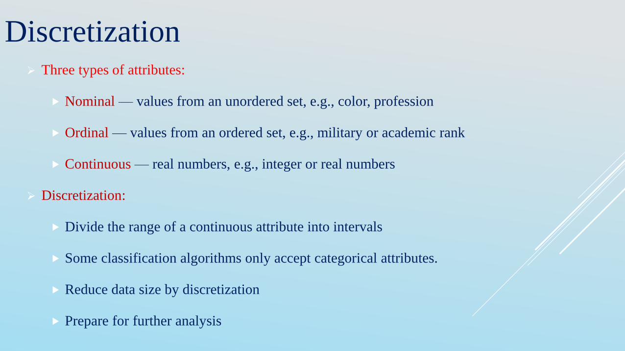
Discretization Three types of attributes:

Nominal — values from an unordered set, e.g., color, profession

Ordinal — values from an ordered set, e.g., military or academic rank

Continuous — real numbers, e.g., integer or real numbers

Discretization:

Divide the range of a continuous attribute into intervals

Some classification algorithms only accept categorical attributes.

Reduce data size by discretization

Prepare for further analysis

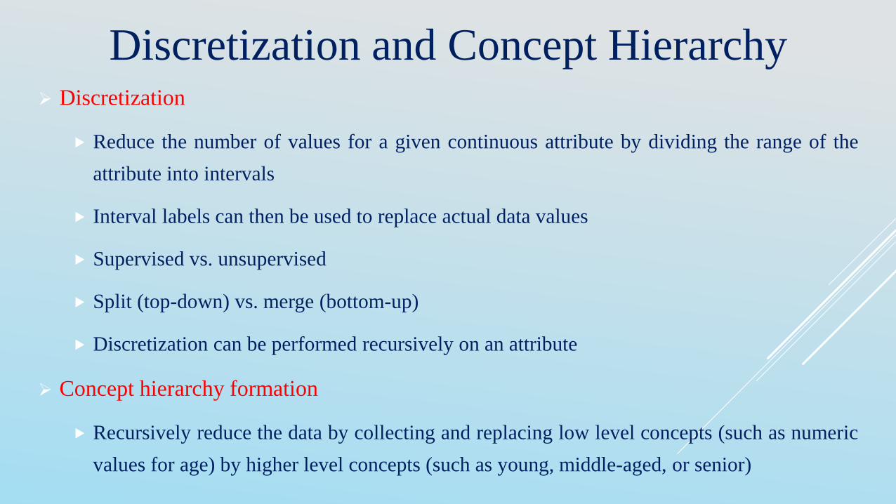
Discretization and Concept Hierarchy Discretization

Reduce the number of values for a given continuous attribute by dividing the range of the

attribute into intervals

Interval labels can then be used to replace actual data values

Supervised vs. unsupervised

Split (top-down) vs. merge (bottom-up)

Discretization can be performed recursively on an attribute

Concept hierarchy formation

Recursively reduce the data by collecting and replacing low level concepts (such as numeric

values for age) by higher level concepts (such as young, middle-aged, or senior)

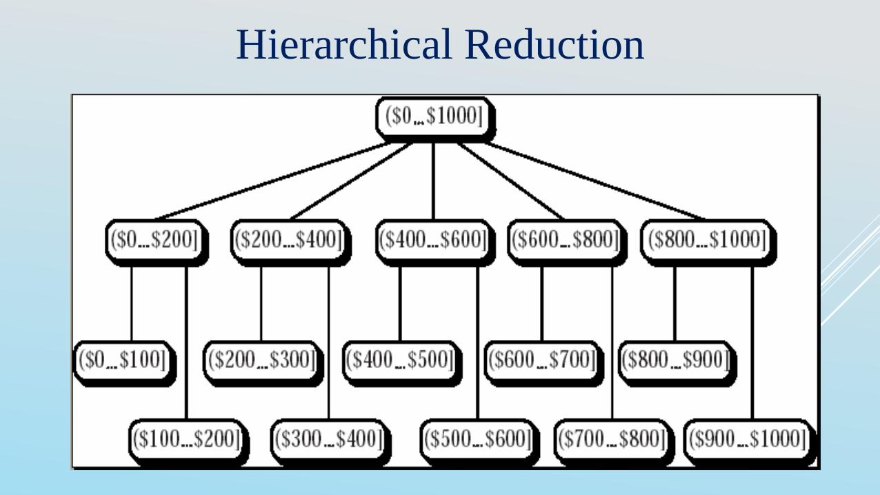
Hierarchical Reduction

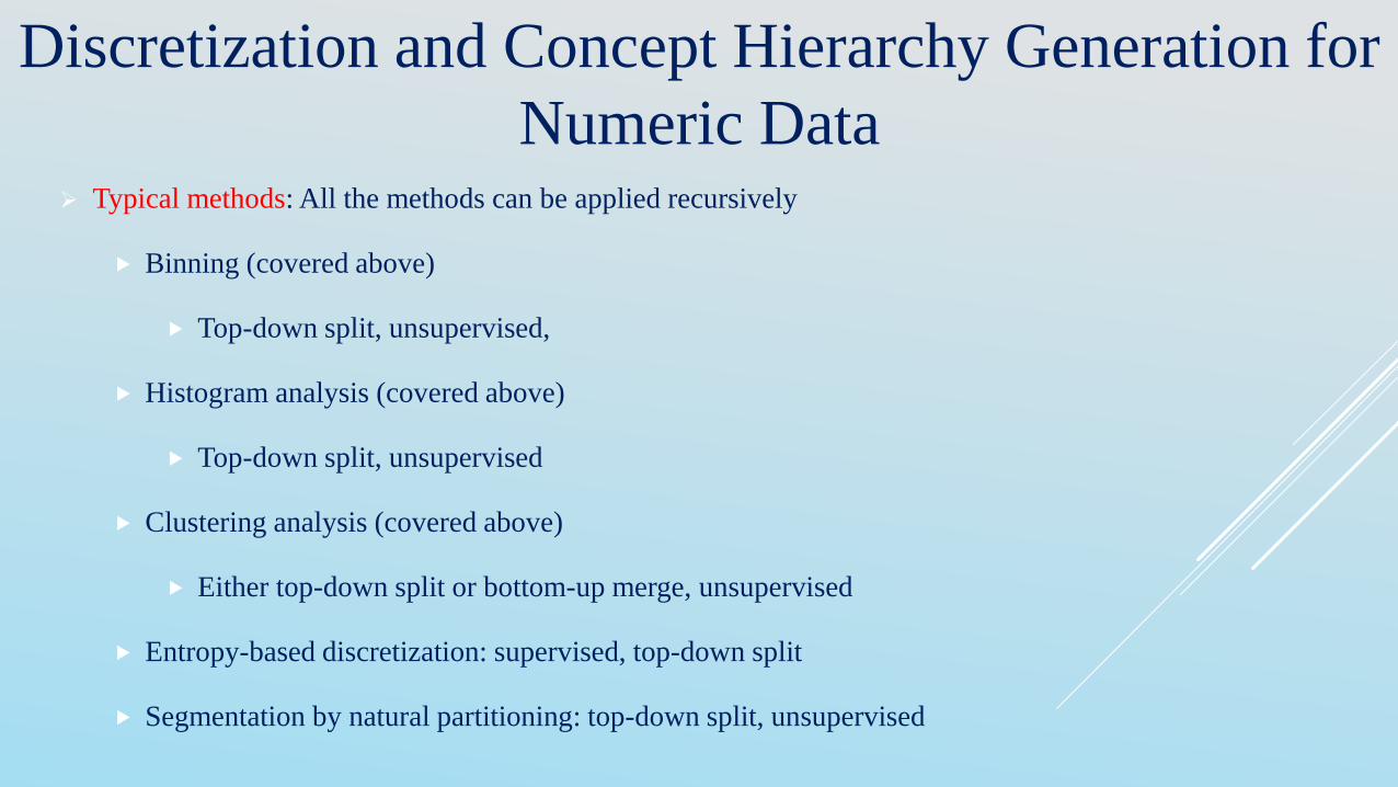
Discretization and Concept Hierarchy Generation for

Numeric Data Typical methods: All the methods can be applied recursively

Binning (covered above)

Top-down split, unsupervised,

Histogram analysis (covered above)

Top-down split, unsupervised

Clustering analysis (covered above)

Either top-down split or bottom-up merge, unsupervised

Entropy-based discretization: supervised, top-down split

Segmentation by natural partitioning: top-down split, unsupervised

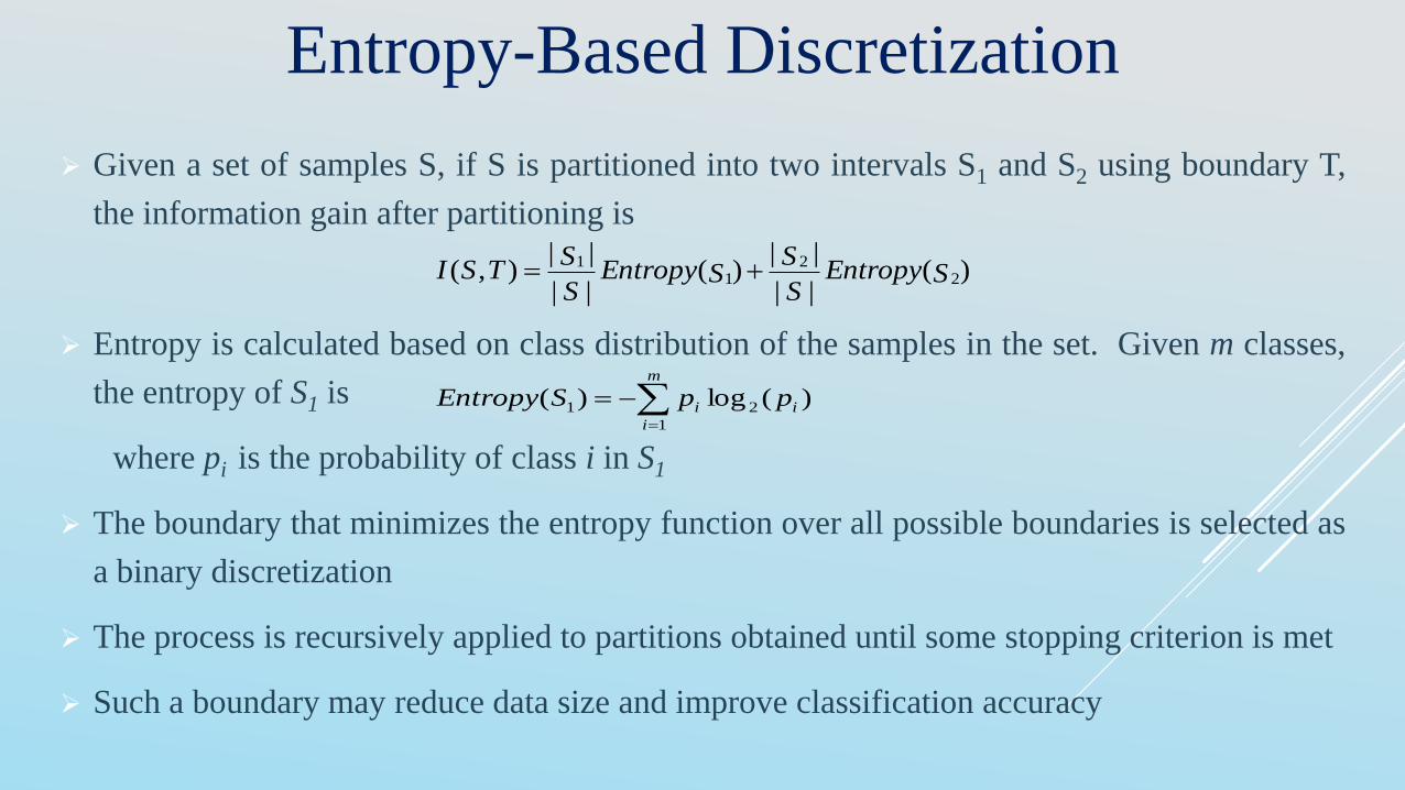
Entropy-Based Discretization

Given a set of samples S, if S is partitioned into two intervals S1 and S2 using boundary T,

the information gain after partitioning is

Entropy is calculated based on class distribution of the samples in the set. Given m classes,

the entropy of S1 is

where pi is the probability of class i in S1

The boundary that minimizes the entropy function over all possible boundaries is selected as

a binary discretization

The process is recursively applied to partitions obtained until some stopping criterion is met

Such a boundary may reduce data size and improve classification accuracy

)(||

||)(

||

||),( 2

21

1SEntropy

S

SSEntropy

S

STSI

m

i

ii ppSEntropy1

21 )(log)(

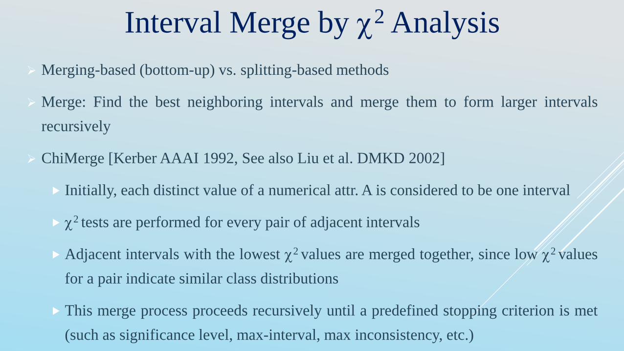
Interval Merge by 2 Analysis

Merging-based (bottom-up) vs. splitting-based methods

Merge: Find the best neighboring intervals and merge them to form larger intervals

recursively

ChiMerge [Kerber AAAI 1992, See also Liu et al. DMKD 2002]

Initially, each distinct value of a numerical attr. A is considered to be one interval

2 tests are performed for every pair of adjacent intervals

Adjacent intervals with the lowest 2 values are merged together, since low 2 values

for a pair indicate similar class distributions

This merge process proceeds recursively until a predefined stopping criterion is met

(such as significance level, max-interval, max inconsistency, etc.)

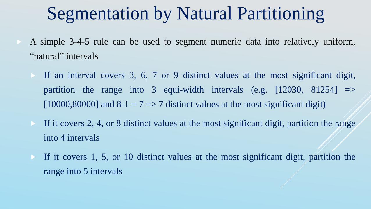
Segmentation by Natural Partitioning

A simple 3-4-5 rule can be used to segment numeric data into relatively uniform,

“natural” intervals.

If an interval covers 3, 6, 7 or 9 distinct values at the most significant digit,

partition the range into 3 equi-width intervals (e.g. [12030, 81254] =>

[10000,80000] and 8-1 = 7 => 7 distinct values at the most significant digit)

If it covers 2, 4, or 8 distinct values at the most significant digit, partition the range

into 4 intervals

If it covers 1, 5, or 10 distinct values at the most significant digit, partition the

range into 5 intervals

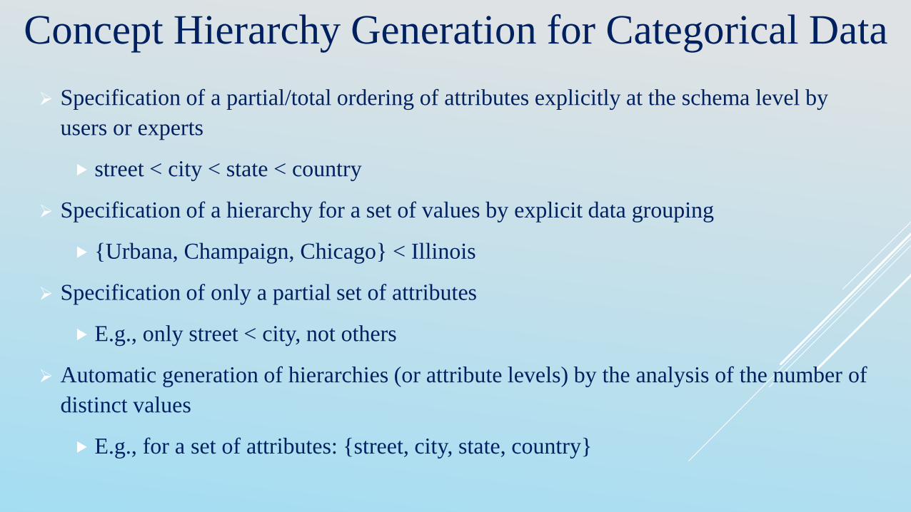
Concept Hierarchy Generation for Categorical Data

Specification of a partial/total ordering of attributes explicitly at the schema level by

users or experts

street < city < state < country

Specification of a hierarchy for a set of values by explicit data grouping

{Urbana, Champaign, Chicago} < Illinois

Specification of only a partial set of attributes

E.g., only street < city, not others

Automatic generation of hierarchies (or attribute levels) by the analysis of the number of

distinct values

E.g., for a set of attributes: {street, city, state, country}

Automatic Concept Hierarchy Generation

Some hierarchies can be automatically generated based on the analysis of the number of distinct values per attribute in the data set

The attribute with the most distinct values is placed at the lowest level of the hierarchy

Exceptions, e.g., weekday, month, quarter, year

country

province or state

city

street

15 distinct values

365 distinct values

3567 distinct values

674,339 distinct values

References

Data preprocessing ppt by Prof. Deepak Moud, Poornima Group of Colleges.

D. P. Ballou and G. K. Tayi. Enhancing data quality in data warehouse environments. Communications of ACM, 42:73-78, 1999

T. Dasu and T. Johnson. Exploratory Data Mining and Data Cleaning. John Wiley & Sons, 2003

T. Dasu, T. Johnson, S. Muthukrishnan, V. Shkapenyuk. Mining Database Structure; Or, How to Build a Data Quality Browser.

SIGMOD’02.

H.V. Jagadish et al., Special Issue on Data Reduction Techniques. Bulletin of the Technical Committee on Data Engineering, 20(4),

December 1997

D. Pyle. Data Preparation for Data Mining. Morgan Kaufmann, 1999

E. Rahm and H. H. Do. Data Cleaning: Problems and Current Approaches. IEEE Bulletin of the Technical Committee on Data Engineering.

Vol.23, No.4

V. Raman and J. Hellerstein. Potters Wheel: An Interactive Framework for Data Cleaning and Transformation, VLDB’2001

T. Redman. Data Quality: Management and Technology. Bantam Books, 1992

Y. Wand and R. Wang. Anchoring data quality dimensions ontological foundations. Communications of ACM, 39:86-95, 1996

R. Wang, V. Storey, and C. Firth. A framework for analysis of data quality research. IEEE Trans. Knowledge and Data Engineering, 7:623-

640, 1995