1 Data Mining Techniques: Frequent Patterns in Sets and Sequences Mirek Riedewald Some slides based on presentations by Han/Kamber and Tan/Steinbach/Kumar Frequent Pattern Mining Overview • Basic Concepts and Challenges • Efficient and Scalable Methods for Frequent Itemsets and Association Rules • Pattern Interestingness Measures • Sequence Mining 2 What Is Frequent Pattern Analysis? • Find patterns (itemset, sequence, structure, etc.) that occur frequently in a data set • First proposed for frequent itemsets and association rule mining • Motivation: Find inherent regularities in data – What products were often purchased together? – What are the subsequent purchases after buying a PC? – What kinds of DNA are sensitive to a new drug? • Applications – Market basket analysis, cross-marketing, catalog design, sale campaign analysis, Web log (click stream) analysis, DNA sequence analysis 3 Association Rule Mining • Given a set of transactions, find rules that will predict the occurrence of an item based on the occurrences of other items in the transaction 4 Market-Basket transactions TID Items 1 Bread, Milk 2 Bread, Diaper, Beer, Eggs 3 Milk, Diaper, Beer, Coke 4 Bread, Milk, Diaper, Beer 5 Bread, Milk, Diaper, Coke Example of Association Rules {Diaper} {Beer}, {Milk, Bread} {Eggs,Coke}, {Beer, Bread} {Milk}, Implication means co-occurrence, not causality! Definition: Frequent Itemset • Itemset – A collection of one or more items • Example: {Milk, Bread, Diaper} – k-itemset: itemset that contains k items • Support count () – Frequency of occurrence of an itemset – E.g., ({Milk, Bread, Diaper}) = 2 • Support (s) – Fraction of transactions that contain an itemset – E.g., s({Milk, Bread, Diaper}) = 2/5 • Frequent Itemset – An itemset whose support is greater than or equal to a minsup threshold 5 TID Items 1 Bread, Milk 2 Bread, Diaper, Beer, Eggs 3 Milk, Diaper, Beer, Coke 4 Bread, Milk, Diaper, Beer 5 Bread, Milk, Diaper, Coke Definition: Association Rule • Association Rule = implication expression of the form XY, where X and Y are itemsets – Ex.: {Milk, Diaper} {Beer} • Rule Evaluation Metrics – Support (s) = P(XY) • Estimated by fraction of transactions that contain both X and Y – Confidence (c) = P(Y| X) • Estimated by fraction of transactions that contain X and Y among all transactions containing X 6 TID Items 1 Bread, Milk 2 Bread, Diaper, Beer, Eggs 3 Milk, Diaper, Beer, Coke 4 Bread, Milk, Diaper, Beer 5 Bread, Milk, Diaper, Coke Example: Beer } Diaper , Milk { 5 2 | D | ) Beer Diaper, , M ilk ( s 3 2 ) Diaper , M ilk ( ) Beer Diaper, M ilk, ( c

Welcome message from author
This document is posted to help you gain knowledge. Please leave a comment to let me know what you think about it! Share it to your friends and learn new things together.
Transcript

1
Data Mining Techniques: Frequent Patterns in Sets and
Sequences
Mirek Riedewald
Some slides based on presentations by Han/Kamber and Tan/Steinbach/Kumar
Frequent Pattern Mining Overview
• Basic Concepts and Challenges
• Efficient and Scalable Methods for Frequent Itemsets and Association Rules
• Pattern Interestingness Measures
• Sequence Mining
2
What Is Frequent Pattern Analysis?
• Find patterns (itemset, sequence, structure, etc.) that occur frequently in a data set
• First proposed for frequent itemsets and association rule mining
• Motivation: Find inherent regularities in data – What products were often purchased together? – What are the subsequent purchases after buying a PC? – What kinds of DNA are sensitive to a new drug?
• Applications – Market basket analysis, cross-marketing, catalog design,
sale campaign analysis, Web log (click stream) analysis, DNA sequence analysis
3
Association Rule Mining
• Given a set of transactions, find rules that will predict the occurrence of an item based on the occurrences of other items in the transaction
4
Market-Basket transactions
TID Items
1 Bread, Milk
2 Bread, Diaper, Beer, Eggs
3 Milk, Diaper, Beer, Coke
4 Bread, Milk, Diaper, Beer
5 Bread, Milk, Diaper, Coke
Example of Association Rules
{Diaper} {Beer},
{Milk, Bread} {Eggs,Coke},
{Beer, Bread} {Milk},
Implication means co-occurrence,
not causality!
Definition: Frequent Itemset
• Itemset – A collection of one or more items
• Example: {Milk, Bread, Diaper}
– k-itemset: itemset that contains k items
• Support count () – Frequency of occurrence of an itemset – E.g., ({Milk, Bread, Diaper}) = 2
• Support (s) – Fraction of transactions that contain an
itemset – E.g., s({Milk, Bread, Diaper}) = 2/5
• Frequent Itemset – An itemset whose support is greater than
or equal to a minsup threshold
5
TID Items
1 Bread, Milk
2 Bread, Diaper, Beer, Eggs
3 Milk, Diaper, Beer, Coke
4 Bread, Milk, Diaper, Beer
5 Bread, Milk, Diaper, Coke
Definition: Association Rule
• Association Rule = implication expression of the form XY, where X and Y are itemsets – Ex.: {Milk, Diaper} {Beer}
• Rule Evaluation Metrics – Support (s) = P(XY)
• Estimated by fraction of transactions that contain both X and Y
– Confidence (c) = P(Y| X) • Estimated by fraction of
transactions that contain X and Y among all transactions containing X
6
TID Items
1 Bread, Milk
2 Bread, Diaper, Beer, Eggs
3 Milk, Diaper, Beer, Coke
4 Bread, Milk, Diaper, Beer
5 Bread, Milk, Diaper, Coke
Example: Beer}Diaper,Milk{
5
2
|D|
)BeerDiaper,,Milk(
s
3
2
)Diaper,Milk(
)BeerDiaper,Milk,(
c
2
Association Rule Mining Task
• Given a transaction database DB, find all rules having support ≥ minsup and confidence ≥ minconf
• Brute-force approach: – List all possible association rules
– Compute support and confidence for each rule
– Remove rules that fail the minsup or minconf thresholds
– Computationally prohibitive!
7
Mining Association Rules
Observations: • All the above rules are binary partitions of the same itemset
{Milk, Diaper, Beer} • Rules originating from the same itemset have identical support but
can have different confidence • Thus, we may decouple the support and confidence requirements
8
TID Items
1 Bread, Milk
2 Bread, Diaper, Beer, Eggs
3 Milk, Diaper, Beer, Coke
4 Bread, Milk, Diaper, Beer
5 Bread, Milk, Diaper, Coke
Example rules:
{Milk,Diaper} {Beer} (s=0.4, c=0.67)
{Milk,Beer} {Diaper} (s=0.4, c=1.0)
{Diaper,Beer} {Milk} (s=0.4, c=0.67)
{Beer} {Milk,Diaper} (s=0.4, c=0.67)
{Diaper} {Milk,Beer} (s=0.4, c=0.5)
{Milk} {Diaper,Beer} (s=0.4, c=0.5)
Mining Association Rules
• Two-step approach:
1. Frequent Itemset Generation
• Generate all itemsets that have support minsup
2. Rule Generation
• Generate high-confidence rules from each frequent itemset, where each rule is a binary partitioning of the frequent itemset
• Frequent itemset generation is still computationally expensive
9
Frequent Itemset Generation
10
null
AB AC AD AE BC BD BE CD CE DE
A B C D E
ABC ABD ABE ACD ACE ADE BCD BCE BDE CDE
ABCD ABCE ABDE ACDE BCDE
ABCDE
Given d items, there
are 2d possible
candidate itemsets
Frequent Itemset Generation
• Brute-force approach: – Each itemset in the lattice is a candidate frequent itemset – Count the support of each candidate by scanning the
database – Match each transaction against every candidate – Complexity O(N*M*w) => expensive since M=2d
11
TID Items
1 Bread, Milk
2 Bread, Diaper, Beer, Eggs
3 Milk, Diaper, Beer, Coke
4 Bread, Milk, Diaper, Beer
5 Bread, Milk, Diaper, Coke
N
Transactions List of
Candidates
M
w
Computational Complexity
• Given d unique items, total number of itemsets = 2d
• Total number of possible association rules?
12
123 1
1
1 1
dd
d
k
kd
j j
kd
k
dR
If d=6, R = 602 possible
rules
3
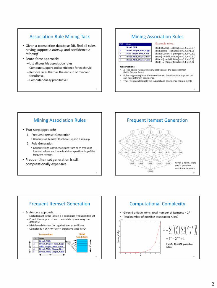
Frequent Pattern Mining Overview
• Basic Concepts and Challenges
• Efficient and Scalable Methods for Frequent Itemsets and Association Rules
• Pattern Interestingness Measures
• Sequence Mining
13
Reducing Number of Candidates
• Apriori principle: – If an itemset is frequent, then all of its subsets must
also be frequent
• Apriori principle holds due to the following property of the support measure: – Support of an itemset never exceeds the support of its
subsets – This is known as the anti-monotone property of
support
14
)()()(:, YsXsYXYX
Illustrating the Apriori Principle
15
Found to be
infrequent
null
AB AC AD AE BC BD BE CD CE DE
A B C D E
ABC ABD ABE ACD ACE ADE BCD BCE BDE CDE
ABCD ABCE ABDE ACDE BCDE
ABCDE
null
AB AC AD AE BC BD BE CD CE DE
A B C D E
ABC ABD ABE ACD ACE ADE BCD BCE BDE CDE
ABCD ABCE ABDE ACDE BCDE
ABCDE
Pruned
supersets
Illustrating the Apriori Principle
16
Item Count
Bread 4Coke 2Milk 4Beer 3Diaper 4Eggs 1
Itemset Count
{Bread,Milk} 3{Bread,Beer} 2{Bread,Diaper} 3{Milk,Beer} 2{Milk,Diaper} 3{Beer,Diaper} 3
Itemset Count
{Bread,Milk,Diaper} 3
Items (1-itemsets)
Pairs (2-itemsets) (No need to generate candidates involving Coke or Eggs)
Triplets (3-itemsets) Minimum Support = 3
If every subset is considered, 6C1 + 6C2 + 6C3 = 41 With support-based pruning, 6 + 6 + 1 = 13
Apriori Algorithm
• Generate L1 = frequent itemsets of length k=1
• Repeat until no new frequent itemsets are found
– Generate Ck+1, the length-(k+1) candidate itemsets, from Lk
– Prune candidate itemsets in Ck+1 containing subsets of length k that are not in Lk (and hence infrequent)
– Count support of each remaining candidate by scanning DB; eliminate infrequent ones from Ck+1
– Lk+1=Ck+1; k = k+1
17
Important Details of Apriori
• How to generate candidates? – Step 1: self-joining Lk
– Step 2: pruning
• Example of Candidate-generation for L3={ {a,b,c}, {a,b,d}, {a,c,d}, {a,c,e}, {b,c,d} } – Self-joining L3
• {a,b,c,d} from {a,b,c} and {a,b,d} • {a,c,d,e} from {a,c,d} and {a,c,e}
– Pruning: • {a,c,d,e} is removed because {a,d,e} is not in L3
– C4={ {a,b,c,d} }
18
4
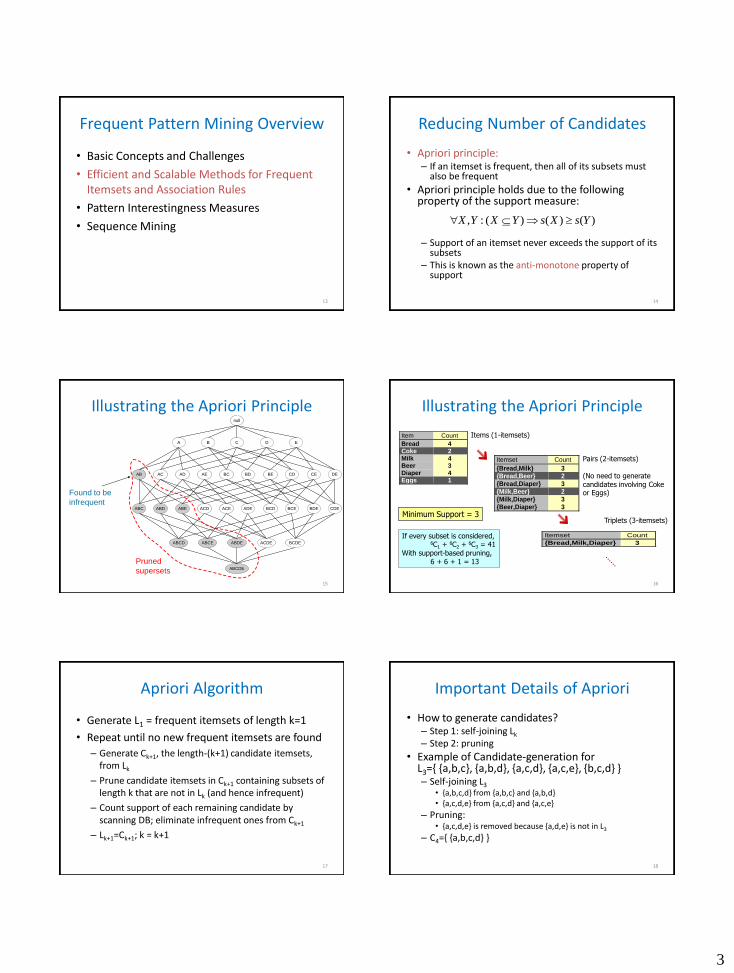
How to Generate Candidates?
• Step 1: self-joining Lk-1 insert into Ck
select p.item1, p.item2,…, p.itemk-1, q.itemk-1
from Lk-1 p, Lk-1 q where p.item1=q.item1 AND … AND p.itemk-2=q.itemk-2
AND p.itemk-1 < q.itemk-1
• Step 2: pruning
– forall itemsets c in Ck do • forall (k-1)-subsets s of c do
– if (s is not in Lk-1) then delete c from Ck
19
How to Count Supports of Candidates?
• Why is counting supports of candidates a problem? – Total number of candidates can be very large – One transaction may contain many candidates
• Method:
– Candidate itemsets stored in a hash-tree – Leaf node contains list of itemsets – Interior node contains a hash table – Subset function finds all candidates contained in a
transaction
20
Generate Hash Tree
• Suppose we have 15 candidate itemsets of length 3: – {1 4 5}, {1 2 4}, {4 5 7}, {1 2 5}, {4 5 8}, {1 5 9}, {1 3 6}, {2 3 4}, {5 6 7}, {3
4 5}, {3 5 6}, {3 5 7}, {6 8 9}, {3 6 7}, {3 6 8}
• We need: – Hash function – Max leaf size: max number of itemsets stored in a leaf node (if number
of candidate itemsets exceeds max leaf size, split the node)
21
2 3 4
5 6 7
1 4 5 1 3 6
1 2 4
4 5 7 1 2 5
4 5 8
1 5 9
3 4 5 3 5 6
3 5 7
6 8 9
3 6 7
3 6 8
1,4,7
2,5,8
3,6,9
Hash function
Subset Operation Using Hash Tree
22
1 5 9
1 4 5 1 3 6
3 4 5 3 6 7
3 6 8
3 5 6
3 5 7
6 8 9
2 3 4
5 6 7
1 2 4
4 5 7
1 2 5
4 5 8
1 2 3 5 6
1 + 2 3 5 6 3 5 6 2 +
5 6 3 +
1,4,7
2,5,8
3,6,9
Hash Function transaction
Subset Operation Using Hash Tree
23
1 5 9
1 4 5 1 3 6
3 4 5 3 6 7
3 6 8
3 5 6
3 5 7
6 8 9
2 3 4
5 6 7
1 2 4
4 5 7
1 2 5
4 5 8
1,4,7
2,5,8
3,6,9
Hash Function 1 2 3 5 6
3 5 6 1 2 +
5 6 1 3 +
6 1 5 +
3 5 6 2 +
5 6 3 +
1 + 2 3 5 6
transaction
Subset Operation Using Hash Tree
24
1 5 9
1 4 5 1 3 6
3 4 5 3 6 7
3 6 8
3 5 6
3 5 7
6 8 9
2 3 4
5 6 7
1 2 4
4 5 7
1 2 5
4 5 8
1,4,7
2,5,8
3,6,9
Hash Function 1 2 3 5 6
3 5 6 1 2 +
5 6 1 3 +
6 1 5 +
3 5 6 2 +
5 6 3 +
1 + 2 3 5 6
transaction
Match transaction against 9 out of 15 candidates
5
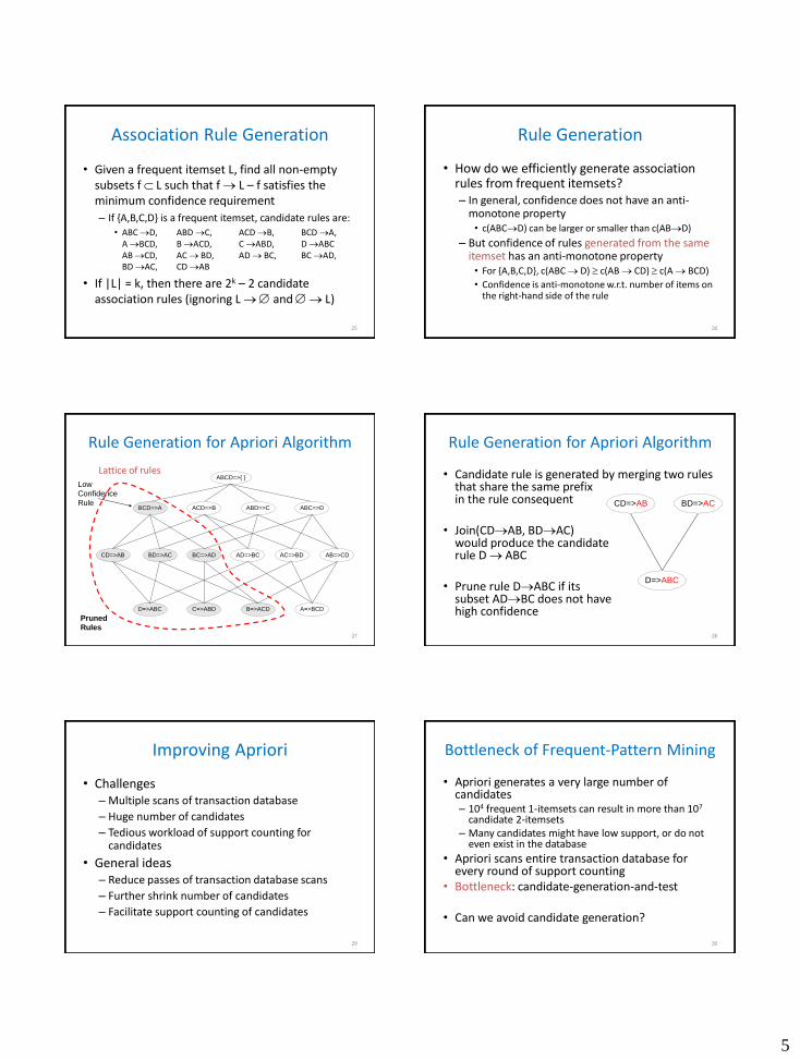
Association Rule Generation
• Given a frequent itemset L, find all non-empty subsets f L such that f L – f satisfies the minimum confidence requirement
– If {A,B,C,D} is a frequent itemset, candidate rules are: • ABC D, ABD C, ACD B, BCD A,
A BCD, B ACD, C ABD, D ABC AB CD, AC BD, AD BC, BC AD, BD AC, CD AB
• If |L| = k, then there are 2k – 2 candidate association rules (ignoring L and L)
25
Rule Generation
• How do we efficiently generate association rules from frequent itemsets? – In general, confidence does not have an anti-
monotone property • c(ABCD) can be larger or smaller than c(ABD)
– But confidence of rules generated from the same itemset has an anti-monotone property
• For {A,B,C,D}, c(ABC D) c(AB CD) c(A BCD)
• Confidence is anti-monotone w.r.t. number of items on the right-hand side of the rule
26
Rule Generation for Apriori Algorithm
27
Lattice of rules ABCD=>{ }
BCD=>A ACD=>B ABD=>C ABC=>D
BC=>ADBD=>ACCD=>AB AD=>BC AC=>BD AB=>CD
D=>ABC C=>ABD B=>ACD A=>BCD
Pruned
Rules
Low
Confidence
Rule
Rule Generation for Apriori Algorithm
• Candidate rule is generated by merging two rules that share the same prefix in the rule consequent
• Join(CDAB, BDAC) would produce the candidate rule D ABC
• Prune rule DABC if its subset ADBC does not have high confidence
28
BD=>ACCD=>AB
D=>ABC
Improving Apriori
• Challenges – Multiple scans of transaction database
– Huge number of candidates
– Tedious workload of support counting for candidates
• General ideas – Reduce passes of transaction database scans
– Further shrink number of candidates
– Facilitate support counting of candidates
29
Bottleneck of Frequent-Pattern Mining
• Apriori generates a very large number of candidates – 104 frequent 1-itemsets can result in more than 107
candidate 2-itemsets – Many candidates might have low support, or do not
even exist in the database
• Apriori scans entire transaction database for every round of support counting
• Bottleneck: candidate-generation-and-test
• Can we avoid candidate generation?
30

6
How to Avoid Candidate Generation
• Grow long patterns from short ones using local frequent items
– Assume {a,b,c} is a frequent pattern in transaction database DB
– Get all transactions containing {a,b,c}
• Notation: DB|{a,b,c}
– {d} is a local frequent item in DB|{a,b,c}, if and only if {a,b,c,d} is a frequent pattern in DB
31
Construct FP-tree from a Transaction Database
32
{} Header Table Item frequency head f 4 c 4 a 3 b 3 m 3 p 3
min_support = 3
TID Items bought (ordered) frequent items 100 {f, a, c, d, g, i, m, p} {f, c, a, m, p} 200 {a, b, c, f, l, m, o} {f, c, a, b, m} 300 {b, f, h, j, o, w} {f, b} 400 {b, c, k, s, p} {c, b, p} 500 {a, f, c, e, l, p, m, n} {f, c, a, m, p}
1. Scan DB once, find frequent 1-itemsets (single item pattern)
2. Sort frequent items in frequency descending order, get f-list
3. Scan DB again, construct FP-tree
F-list=f-c-a-b-m-p
Construct FP-tree from a Transaction Database
33
{}
f:1
c:1
a:1
m:1
p:1
Header Table Item frequency head f 4 c 4 a 3 b 3 m 3 p 3
min_support = 3
TID Items bought (ordered) frequent items 100 {f, a, c, d, g, i, m, p} {f, c, a, m, p} 200 {a, b, c, f, l, m, o} {f, c, a, b, m} 300 {b, f, h, j, o, w} {f, b} 400 {b, c, k, s, p} {c, b, p} 500 {a, f, c, e, l, p, m, n} {f, c, a, m, p}
1. Scan DB once, find frequent 1-itemsets (single item pattern)
2. Sort frequent items in frequency descending order, get f-list
3. Scan DB again, construct FP-tree
F-list=f-c-a-b-m-p
Construct FP-tree from a Transaction Database
34
{}
f:2
c:2
a:2
b:1 m:1
p:1 m:1
Header Table Item frequency head f 4 c 4 a 3 b 3 m 3 p 3
min_support = 3
TID Items bought (ordered) frequent items 100 {f, a, c, d, g, i, m, p} {f, c, a, m, p} 200 {a, b, c, f, l, m, o} {f, c, a, b, m} 300 {b, f, h, j, o, w} {f, b} 400 {b, c, k, s, p} {c, b, p} 500 {a, f, c, e, l, p, m, n} {f, c, a, m, p}
1. Scan DB once, find frequent 1-itemsets (single item pattern)
2. Sort frequent items in frequency descending order, get f-list
3. Scan DB again, construct FP-tree
F-list=f-c-a-b-m-p
Construct FP-tree from a Transaction Database
35
{}
f:4 c:1
b:1
p:1
b:1 c:3
a:3
b:1 m:2
p:2 m:1
Header Table Item frequency head f 4 c 4 a 3 b 3 m 3 p 3
min_support = 3
TID Items bought (ordered) frequent items 100 {f, a, c, d, g, i, m, p} {f, c, a, m, p} 200 {a, b, c, f, l, m, o} {f, c, a, b, m} 300 {b, f, h, j, o, w} {f, b} 400 {b, c, k, s, p} {c, b, p} 500 {a, f, c, e, l, p, m, n} {f, c, a, m, p}
1. Scan DB once, find frequent 1-itemsets (single item pattern)
2. Sort frequent items in frequency descending order, get f-list
3. Scan DB again, construct FP-tree
F-list=f-c-a-b-m-p
Benefits of the FP-tree Structure
• Completeness – Preserve complete information for frequent pattern
mining – Never break a long pattern of any transaction
• Compactness – Reduce irrelevant info—infrequent items are gone – Items in frequency descending order: the more
frequently occurring, the more likely to be shared – Never larger than the original database (if we do not
count node-links and the count field) – For some example DBs, compression ratio over 100
36
7
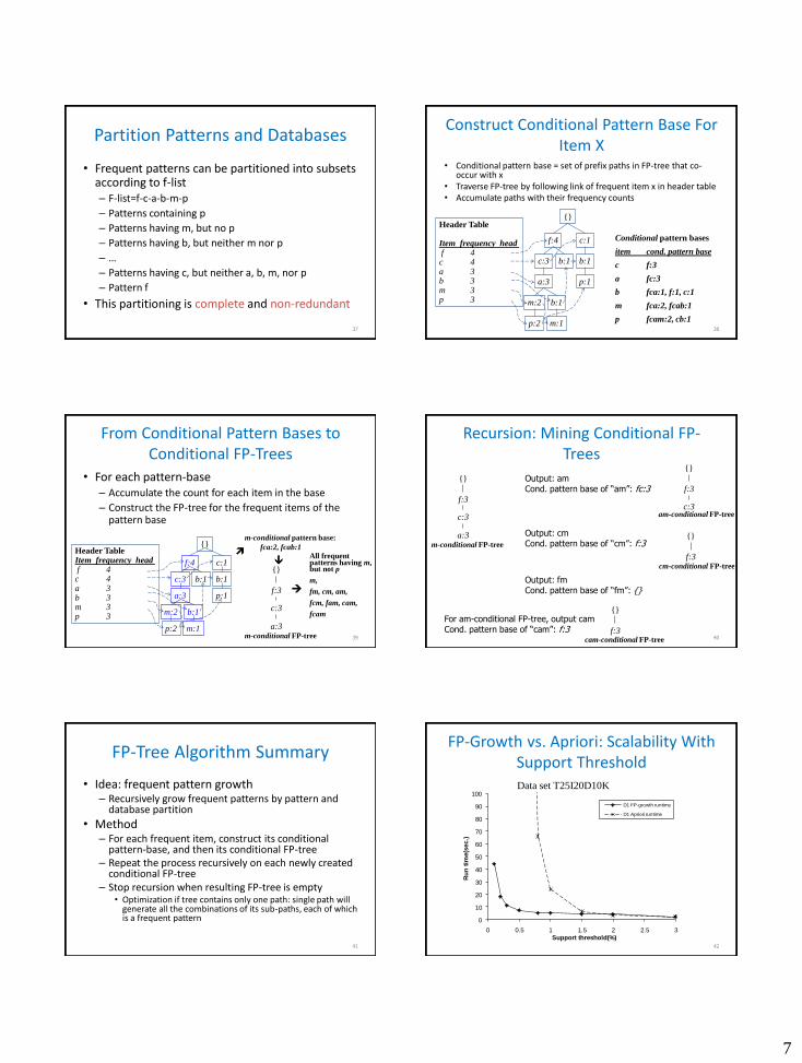
Partition Patterns and Databases
• Frequent patterns can be partitioned into subsets according to f-list – F-list=f-c-a-b-m-p
– Patterns containing p
– Patterns having m, but no p
– Patterns having b, but neither m nor p
– …
– Patterns having c, but neither a, b, m, nor p
– Pattern f
• This partitioning is complete and non-redundant
37
Construct Conditional Pattern Base For Item X
• Conditional pattern base = set of prefix paths in FP-tree that co-occur with x
• Traverse FP-tree by following link of frequent item x in header table • Accumulate paths with their frequency counts
38
Conditional pattern bases
item cond. pattern base
c f:3
a fc:3
b fca:1, f:1, c:1
m fca:2, fcab:1
p fcam:2, cb:1
{}
f:4 c:1
b:1
p:1
b:1 c:3
a:3
b:1 m:2
p:2 m:1
Header Table Item frequency head f 4 c 4 a 3 b 3 m 3 p 3
From Conditional Pattern Bases to Conditional FP-Trees
• For each pattern-base – Accumulate the count for each item in the base
– Construct the FP-tree for the frequent items of the pattern base
39
m-conditional pattern base:
fca:2, fcab:1
{}
f:3
c:3
a:3 m-conditional FP-tree
All frequent patterns having m, but not p
m,
fm, cm, am,
fcm, fam, cam,
fcam
{}
f:4 c:1
b:1
p:1
b:1 c:3
a:3
b:1 m:2
p:2 m:1
Header Table Item frequency head f 4 c 4 a 3 b 3 m 3 p 3
Recursion: Mining Conditional FP-Trees
40
{}
f:3
c:3
a:3 m-conditional FP-tree
Output: am Cond. pattern base of “am”: fc:3
{}
f:3
c:3 am-conditional FP-tree
Output: cm Cond. pattern base of “cm”: f:3
{}
f:3 cm-conditional FP-tree
For am-conditional FP-tree, output cam Cond. pattern base of “cam”: f:3
{}
f:3 cam-conditional FP-tree
Output: fm Cond. pattern base of “fm”: {}
FP-Tree Algorithm Summary
• Idea: frequent pattern growth – Recursively grow frequent patterns by pattern and
database partition
• Method – For each frequent item, construct its conditional
pattern-base, and then its conditional FP-tree – Repeat the process recursively on each newly created
conditional FP-tree – Stop recursion when resulting FP-tree is empty
• Optimization if tree contains only one path: single path will generate all the combinations of its sub-paths, each of which is a frequent pattern
41
FP-Growth vs. Apriori: Scalability With Support Threshold
42
0
10
20
30
40
50
60
70
80
90
100
0 0.5 1 1.5 2 2.5 3
Ru
n t
ime(s
ec.)
Support threshold(%)
D1 FP-growth runtime
D1 Apriori runtime
Data set T25I20D10K

8
Why Is FP-Growth the Winner?
• Divide-and-conquer – Decompose both the mining task and DB according to
the frequent patterns obtained so far – Leads to focused search of smaller databases
• Other factors – No candidate generation, no candidate test – Compressed database: FP-tree structure – No repeated scan of entire database – Basic operations: counting local frequent single items
and building sub FP-tree • No pattern search and matching
43
Factors Affecting Mining Cost
• Choice of minimum support threshold – Lower support threshold => more frequent itemsets
• More candidates, longer frequent itemsets
• Dimensionality (number of items) of the data set – More space needed to store support count of each item – If number of frequent items also increases, both computation and I/O
costs may increase
• Size of database – Each pass over DB is more expensive
• Average transaction width – May increase max. length of frequent itemsets and traversals of hash
tree (more subsets supported by transaction)
• How can we further reduce some of these costs?
44
Compact Representation of Frequent Itemsets
• Some itemsets are redundant because they have identical support as their supersets
• Number of frequent itemsets
• Need a compact representation
45
TID A1 A2 A3 A4 A5 A6 A7 A8 A9 A10 B1 B2 B3 B4 B5 B6 B7 B8 B9 B10 C1 C2 C3 C4 C5 C6 C7 C8 C9 C10
1 1 1 1 1 1 1 1 1 1 1 0 0 0 0 0 0 0 0 0 0 0 0 0 0 0 0 0 0 0 0
2 1 1 1 1 1 1 1 1 1 1 0 0 0 0 0 0 0 0 0 0 0 0 0 0 0 0 0 0 0 0
3 1 1 1 1 1 1 1 1 1 1 0 0 0 0 0 0 0 0 0 0 0 0 0 0 0 0 0 0 0 0
4 1 1 1 1 1 1 1 1 1 1 0 0 0 0 0 0 0 0 0 0 0 0 0 0 0 0 0 0 0 0
5 1 1 1 1 1 1 1 1 1 1 0 0 0 0 0 0 0 0 0 0 0 0 0 0 0 0 0 0 0 0
6 0 0 0 0 0 0 0 0 0 0 1 1 1 1 1 1 1 1 1 1 0 0 0 0 0 0 0 0 0 0
7 0 0 0 0 0 0 0 0 0 0 1 1 1 1 1 1 1 1 1 1 0 0 0 0 0 0 0 0 0 0
8 0 0 0 0 0 0 0 0 0 0 1 1 1 1 1 1 1 1 1 1 0 0 0 0 0 0 0 0 0 0
9 0 0 0 0 0 0 0 0 0 0 1 1 1 1 1 1 1 1 1 1 0 0 0 0 0 0 0 0 0 0
10 0 0 0 0 0 0 0 0 0 0 1 1 1 1 1 1 1 1 1 1 0 0 0 0 0 0 0 0 0 0
11 0 0 0 0 0 0 0 0 0 0 0 0 0 0 0 0 0 0 0 0 1 1 1 1 1 1 1 1 1 1
12 0 0 0 0 0 0 0 0 0 0 0 0 0 0 0 0 0 0 0 0 1 1 1 1 1 1 1 1 1 1
13 0 0 0 0 0 0 0 0 0 0 0 0 0 0 0 0 0 0 0 0 1 1 1 1 1 1 1 1 1 1
14 0 0 0 0 0 0 0 0 0 0 0 0 0 0 0 0 0 0 0 0 1 1 1 1 1 1 1 1 1 1
15 0 0 0 0 0 0 0 0 0 0 0 0 0 0 0 0 0 0 0 0 1 1 1 1 1 1 1 1 1 1
10
1
103
k k
Maximal Frequent Itemset
46
null
AB AC AD AE BC BD BE CD CE DE
A B C D E
ABC ABD ABE ACD ACE ADE BCD BCE BDE CDE
ABCD ABCE ABDE ACDE BCDE
ABCD
E
Border
Infrequent
Itemsets
Maximal
Itemsets
An itemset is maximal-frequent if none of its supersets is frequent
Closed Itemset
• A frequent itemset is closed if none of its supersets has the same support – Lossless compression of the set of all frequent
itemsets
47
TID Items
1 {A,B}
2 {B,C,D}
3 {A,B,C,D}
4 {A,B,D}
5 {A,B,C,D}
Itemset Support
{A} 4
{B} 5
{C} 3
{D} 4
{A,B} 4
{A,C} 2
{A,D} 3
{B,C} 3
{B,D} 4
{C,D} 3
Itemset Support
{A,B,C} 2
{A,B,D} 3
{A,C,D} 2
{B,C,D} 3
{A,B,C,D} 2
min_sup = 2
Maximal vs Closed Frequent Itemsets
48
TID Items
1 ABC
2 ABCD
3 BCE
4 ACDE
5 DE
null
AB AC AD AE BC BD BE CD CE DE
A B C D E
ABC ABD ABE ACD ACE ADE BCD BCE BDE CDE
ABCD ABCE ABDE ACDE BCDE
ABCDE
124 123 1234 245 345
12 124 24 4 123 2 3 24 34 45
12 2 24 4 4 2 3 4
2 4
Transaction Ids
Not supported by
any transactions
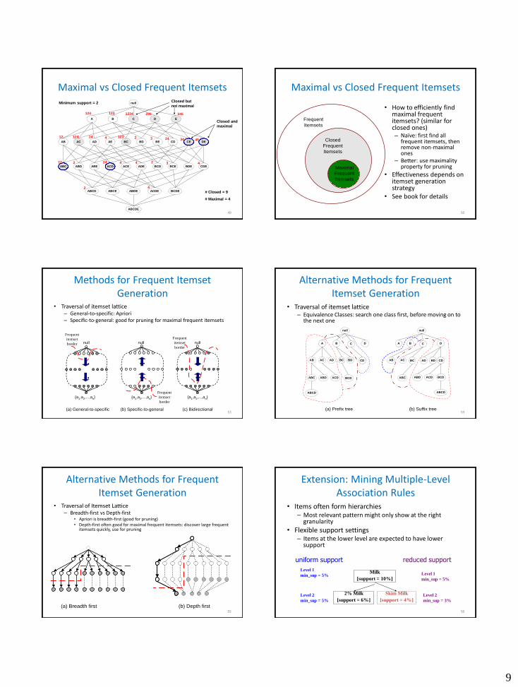
9
Maximal vs Closed Frequent Itemsets
49
null
AB AC AD AE BC BD BE CD CE DE
A B C D E
ABC ABD ABE ACD ACE ADE BCD BCE BDE CDE
ABCD ABCE ABDE ACDE BCDE
ABCDE
124 123 1234 245 345
12 124 24 4 123 2 3 24 34 45
12 2 24 4 4 2 3 4
2 4
Minimum support = 2
# Closed = 9
# Maximal = 4
Closed and
maximal
Closed but
not maximal
Maximal vs Closed Frequent Itemsets
• How to efficiently find maximal frequent itemsets? (similar for closed ones) – Naïve: first find all
frequent itemsets, then remove non-maximal ones
– Better: use maximality property for pruning
• Effectiveness depends on itemset generation strategy
• See book for details
50
Frequent
Itemsets
Closed
Frequent
Itemsets
Maximal
Frequent
Itemsets
Methods for Frequent Itemset Generation
• Traversal of itemset lattice – General-to-specific: Apriori – Specific-to-general: good for pruning for maximal frequent itemsets
53
Frequent
itemset
border null
{a1,a
2,...,a
n}
(a) General-to-specific
null
{a1,a
2,...,a
n}
Frequent
itemset
border
(b) Specific-to-general
..
..
..
..
Frequent
itemset
border
null
{a1,a
2,...,a
n}
(c) Bidirectional
..
..
Alternative Methods for Frequent Itemset Generation
• Traversal of itemset lattice – Equivalence Classes: search one class first, before moving on to
the next one
54
null
AB AC AD BC BD CD
A B C D
ABC ABD ACD BCD
ABCD
null
AB AC ADBC BD CD
A B C D
ABC ABD ACD BCD
ABCD
(a) Prefix tree (b) Suffix tree
Alternative Methods for Frequent Itemset Generation
• Traversal of Itemset Lattice – Breadth-first vs Depth-first
• Apriori is breadth-first (good for pruning) • Depth-first often good for maximal frequent itemsets: discover large frequent
itemsets quickly, use for pruning
55
(a) Breadth first (b) Depth first
Extension: Mining Multiple-Level Association Rules
• Items often form hierarchies – Most relevant pattern might only show at the right
granularity
• Flexible support settings – Items at the lower level are expected to have lower
support
56
uniform support
Milk
[support = 10%]
2% Milk
[support = 6%]
Skim Milk
[support = 4%]
Level 1
min_sup = 5%
Level 2
min_sup = 5%
Level 1
min_sup = 5%
Level 2
min_sup = 3%
reduced support
10
Extension: Mining Multi-Dimensional Associations
• Single-dimensional rules: one type of predicate • buys(X, “milk”) buys(X, “bread”)
• Multi-dimensional rules: 2 types of predicates – Interdimensional association rules (no repeated
predicates) • age(X, “19-25”) occupation(X, “student”) buys(X,
“coke”)
– Hybrid-dimensional association rules (repeated predicates)
• age(X, “19-25”) buys(X, “popcorn”) buys(X, “coke”)
• See book for efficient mining algorithms
57
Frequent Pattern Mining Overview
• Basic Concepts and Challenges
• Efficient and Scalable Methods for Frequent Itemsets and Association Rules
• Pattern Interestingness Measures
• Sequence Mining
58
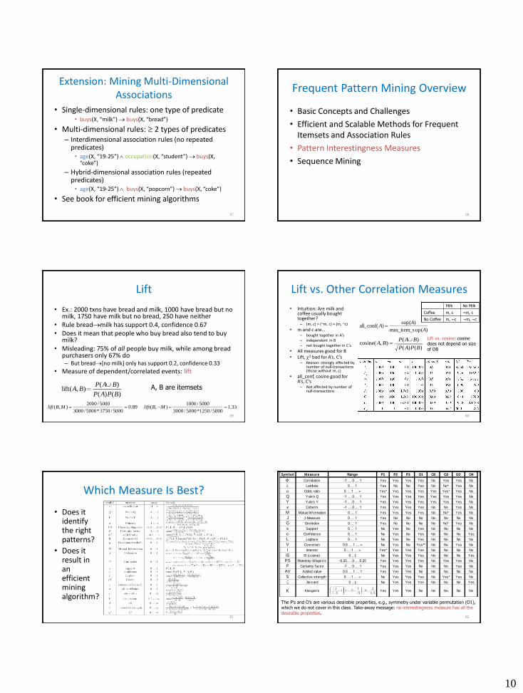
Lift
• Ex.: 2000 txns have bread and milk, 1000 have bread but no milk, 1750 have milk but no bread, 250 have neither
• Rule breadmilk has support 0.4, confidence 0.67 • Does it mean that people who buy bread also tend to buy
milk? • Misleading: 75% of all people buy milk, while among bread
purchasers only 67% do – But bread[no milk] only has support 0.2, confidence 0.33
• Measure of dependent/correlated events: lift
59
89.05000/3750*5000/3000
5000/2000),( MBlift 33.1
5000/1250*5000/3000
5000/1000),( MBlift
)()(
)(),lift(
BPAP
BAPBA
A, B are itemsets
Lift vs. Other Correlation Measures
• Intuition: Are milk and coffee usually bought together?
– (m, c) > (~m, c) + (m, ~c)
• m and c are… – bought together in A’s – independent in B – not bought together in C’s
• All measures good for B • Lift, 2 bad for A’s, C’s
– Reason: strongly affected by number of null-transactions (those without m, c)
• all_conf, cosine good for A’s, C’s
– Not affected by number of null-transactions
60
Milk No Milk
Coffee m, c ~m, c
No Coffee m, ~c ~m, ~c
)up(max_item_s
)sup()all_conf(
A
AA
)()(
)(),cosine(
BPAP
BAPBA
Lift vs. cosine: cosine does not depend on size of DB
Which Measure Is Best?
• Does it identify the right patterns?
• Does it result in an efficient mining algorithm?
61 62
Symbol Measure Range P1 P2 P3 O1 O2 O3 O3' O4
Correlation -1 … 0 … 1 Yes Yes Yes Yes No Yes Yes No
Lambda 0 … 1 Yes No No Yes No No* Yes No
Odds ratio 0 … 1 … Yes* Yes Yes Yes Yes Yes* Yes No
Q Yule's Q -1 … 0 … 1 Yes Yes Yes Yes Yes Yes Yes No
Y Yule's Y -1 … 0 … 1 Yes Yes Yes Yes Yes Yes Yes No
Cohen's -1 … 0 … 1 Yes Yes Yes Yes No No Yes No
M Mutual Information 0 … 1 Yes Yes Yes Yes No No* Yes No
J J-Measure 0 … 1 Yes No No No No No No No
G Gini Index 0 … 1 Yes No No No No No* Yes No
s Support 0 … 1 No Yes No Yes No No No No
c Confidence 0 … 1 No Yes No Yes No No No Yes
L Laplace 0 … 1 No Yes No Yes No No No No
V Conviction 0.5 … 1 … No Yes No Yes** No No Yes No
I Interest 0 … 1 … Yes* Yes Yes Yes No No No No
IS IS (cosine) 0 .. 1 No Yes Yes Yes No No No Yes
PS Piatetsky-Shapiro's -0.25 … 0 … 0.25 Yes Yes Yes Yes No Yes Yes No
F Certainty factor -1 … 0 … 1 Yes Yes Yes No No No Yes No
AV Added value 0.5 … 1 … 1 Yes Yes Yes No No No No No
S Collective strength 0 … 1 … No Yes Yes Yes No Yes* Yes No
Jaccard 0 .. 1 No Yes Yes Yes No No No Yes
K Klosgen's Yes Yes Yes No No No No No33
20
3
1321
3
2
The P’s and O’s are various desirable properties, e.g., symmetry under variable permutation (O1), which we do not cover in this class. Take-away message: no interestingness measure has all the desirable properties.
11
Frequent Pattern Mining Overview
• Basic Concepts and Challenges
• Efficient and Scalable Methods for Frequent Itemsets and Association Rules
• Pattern Interestingness Measures
• Sequence Mining
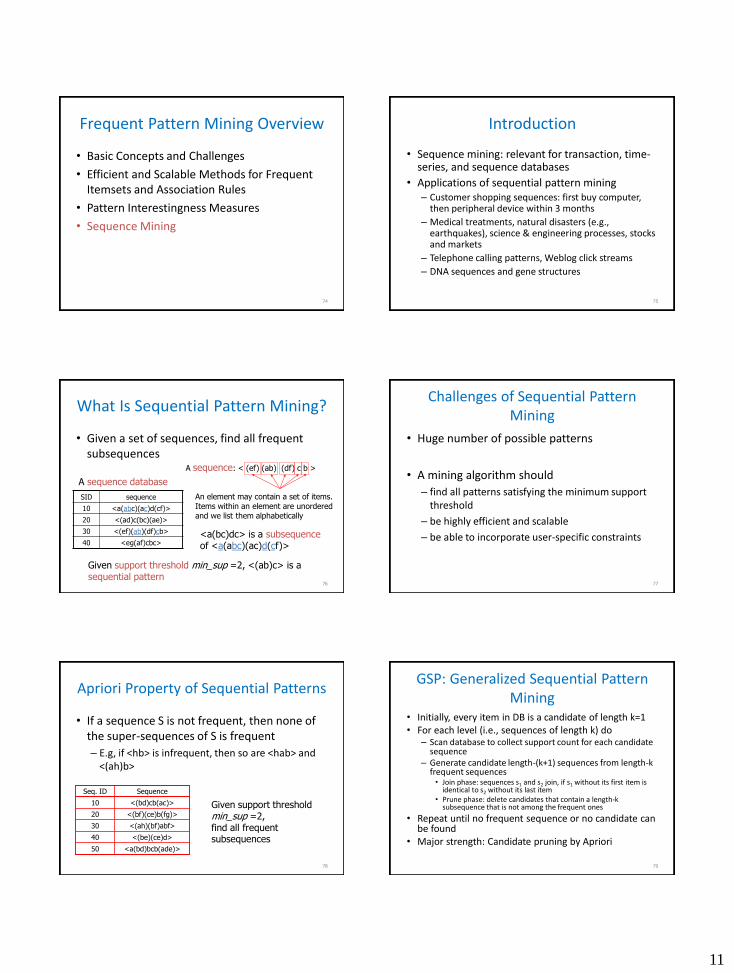
74
Introduction
• Sequence mining: relevant for transaction, time-series, and sequence databases
• Applications of sequential pattern mining – Customer shopping sequences: first buy computer,
then peripheral device within 3 months
– Medical treatments, natural disasters (e.g., earthquakes), science & engineering processes, stocks and markets
– Telephone calling patterns, Weblog click streams
– DNA sequences and gene structures
75
What Is Sequential Pattern Mining?
• Given a set of sequences, find all frequent subsequences
76
A sequence database
A sequence: < (ef) (ab) (df) c b >
An element may contain a set of items. Items within an element are unordered and we list them alphabetically
<a(bc)dc> is a subsequence of <a(abc)(ac)d(cf)>
Given support threshold min_sup =2, <(ab)c> is a sequential pattern
SID sequence
10 <a(abc)(ac)d(cf)>
20 <(ad)c(bc)(ae)>
30 <(ef)(ab)(df)cb>
40 <eg(af)cbc>
Challenges of Sequential Pattern Mining
• Huge number of possible patterns
• A mining algorithm should
– find all patterns satisfying the minimum support threshold
– be highly efficient and scalable
– be able to incorporate user-specific constraints
77
Apriori Property of Sequential Patterns
• If a sequence S is not frequent, then none of the super-sequences of S is frequent
– E.g, if <hb> is infrequent, then so are <hab> and <(ah)b>
78
<a(bd)bcb(ade)> 50
<(be)(ce)d> 40
<(ah)(bf)abf> 30
<(bf)(ce)b(fg)> 20
<(bd)cb(ac)> 10
Sequence Seq. ID
Given support threshold min_sup =2, find all frequent subsequences
GSP: Generalized Sequential Pattern Mining
• Initially, every item in DB is a candidate of length k=1 • For each level (i.e., sequences of length k) do
– Scan database to collect support count for each candidate sequence
– Generate candidate length-(k+1) sequences from length-k frequent sequences
• Join phase: sequences s1 and s2 join, if s1 without its first item is identical to s2 without its last item
• Prune phase: delete candidates that contain a length-k subsequence that is not among the frequent ones
• Repeat until no frequent sequence or no candidate can be found
• Major strength: Candidate pruning by Apriori
79
12
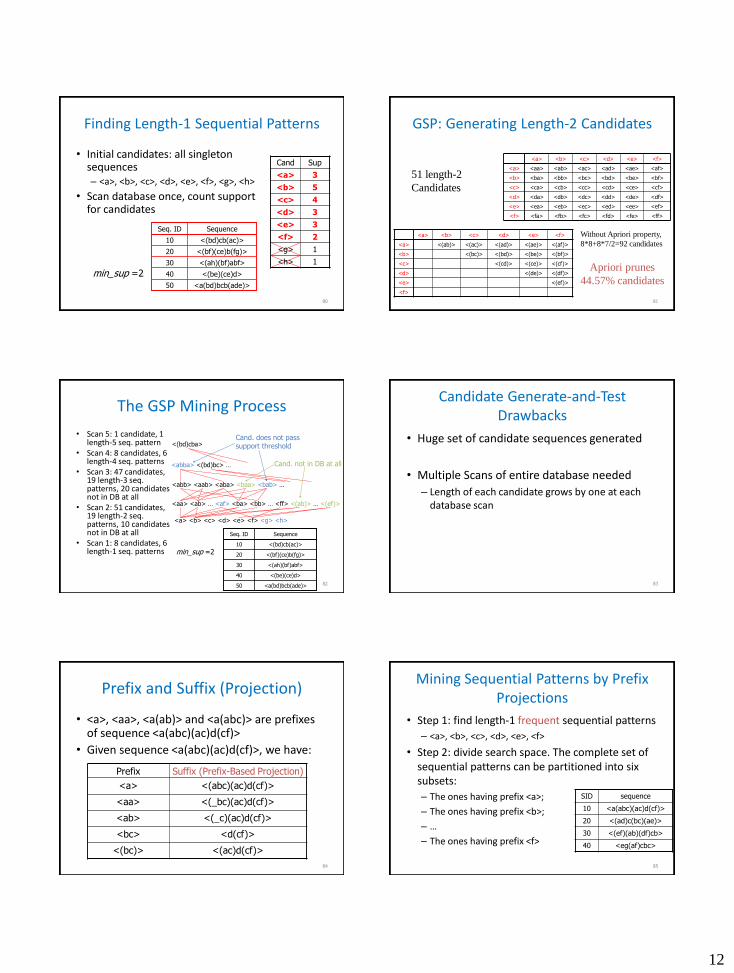
Finding Length-1 Sequential Patterns
• Initial candidates: all singleton sequences – <a>, <b>, <c>, <d>, <e>, <f>, <g>, <h>
• Scan database once, count support for candidates
80
<a(bd)bcb(ade)> 50
<(be)(ce)d> 40
<(ah)(bf)abf> 30
<(bf)(ce)b(fg)> 20
<(bd)cb(ac)> 10
Sequence Seq. ID
min_sup =2
Cand Sup
<a> 3
<b> 5
<c> 4
<d> 3
<e> 3
<f> 2
<g> 1
<h> 1
GSP: Generating Length-2 Candidates
81
<a> <b> <c> <d> <e> <f>
<a> <aa> <ab> <ac> <ad> <ae> <af>
<b> <ba> <bb> <bc> <bd> <be> <bf>
<c> <ca> <cb> <cc> <cd> <ce> <cf>
<d> <da> <db> <dc> <dd> <de> <df>
<e> <ea> <eb> <ec> <ed> <ee> <ef>
<f> <fa> <fb> <fc> <fd> <fe> <ff>
<a> <b> <c> <d> <e> <f>
<a> <(ab)> <(ac)> <(ad)> <(ae)> <(af)>
<b> <(bc)> <(bd)> <(be)> <(bf)>
<c> <(cd)> <(ce)> <(cf)>
<d> <(de)> <(df)>
<e> <(ef)>
<f>
51 length-2
Candidates
Without Apriori property,
8*8+8*7/2=92 candidates
Apriori prunes
44.57% candidates
The GSP Mining Process
• Scan 5: 1 candidate, 1 length-5 seq. pattern
• Scan 4: 8 candidates, 6 length-4 seq. patterns
• Scan 3: 47 candidates, 19 length-3 seq. patterns, 20 candidates not in DB at all
• Scan 2: 51 candidates, 19 length-2 seq. patterns, 10 candidates not in DB at all
• Scan 1: 8 candidates, 6 length-1 seq. patterns
82
<a> <b> <c> <d> <e> <f> <g> <h>
<aa> <ab> … <af> <ba> <bb> … <ff> <(ab)> … <(ef)>
<abb> <aab> <aba> <baa> <bab> …
<abba> <(bd)bc> …
<(bd)cba> Cand. does not pass support threshold
Cand. not in DB at all
min_sup =2
<a(bd)bcb(ade)> 50
<(be)(ce)d> 40
<(ah)(bf)abf> 30
<(bf)(ce)b(fg)> 20
<(bd)cb(ac)> 10
Sequence Seq. ID
Candidate Generate-and-Test Drawbacks
• Huge set of candidate sequences generated
• Multiple Scans of entire database needed
– Length of each candidate grows by one at each database scan
83
Prefix and Suffix (Projection)
• <a>, <aa>, <a(ab)> and <a(abc)> are prefixes of sequence <a(abc)(ac)d(cf)>
• Given sequence <a(abc)(ac)d(cf)>, we have:
84
Prefix Suffix (Prefix-Based Projection)
<a> <(abc)(ac)d(cf)>
<aa> <(_bc)(ac)d(cf)>
<ab> <(_c)(ac)d(cf)>
<bc> <d(cf)>
<(bc)> <(ac)d(cf)>
Mining Sequential Patterns by Prefix Projections
• Step 1: find length-1 frequent sequential patterns
– <a>, <b>, <c>, <d>, <e>, <f>
• Step 2: divide search space. The complete set of sequential patterns can be partitioned into six subsets:
– The ones having prefix <a>;
– The ones having prefix <b>;
– …
– The ones having prefix <f>
85
SID sequence
10 <a(abc)(ac)d(cf)>
20 <(ad)c(bc)(ae)>
30 <(ef)(ab)(df)cb>
40 <eg(af)cbc>

13
Finding Seq. Patterns with Prefix <a>
• Only need to consider projections w.r.t. <a> – <a>-projected database: <(abc)(ac)d(cf)>,
<(_d)c(bc)(ae)>, <(_b)(df)cb>, <(_f)cbc>
• Find all length-2 frequent seq. patterns having prefix <a>: <aa>, <ab>, <(ab)>, <ac>, <ad>, <af> – Further partition into those 6 subsets
• Having prefix <aa>;
• Having prefix <ab>;
• Having prefix <(ab)>;
• …
• Having prefix <af>
86
SID sequence
10 <a(abc)(ac)d(cf)>
20 <(ad)c(bc)(ae)>
30 <(ef)(ab)(df)cb>
40 <eg(af)cbc>
Completeness of PrefixSpan
87
SID sequence
10 <a(abc)(ac)d(cf)>
20 <(ad)c(bc)(ae)>
30 <(ef)(ab)(df)cb>
40 <eg(af)cbc>
DB
Length-1 sequential patterns <a>, <b>, <c>, <d>, <e>, <f>
<a>-projected database <(abc)(ac)d(cf)> <(_d)c(bc)(ae)> <(_b)(df)cb> <(_f)cbc>
Length-2 sequential patterns <aa>, <ab>, <(ab)>, <ac>, <ad>, <af>
Having prefix <a>
Having prefix <aa>
<aa>-proj. db … <af>-proj. db
Having prefix <af>
<b>-projected database …
Having prefix <b>
Having prefix <c>, …, <f>
… …
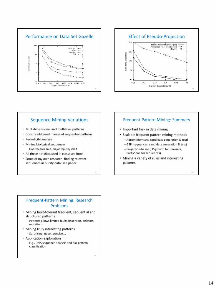
Efficiency of PrefixSpan
• No candidate sequence needs to be generated
• Projected databases keep shrinking
• Major cost of PrefixSpan: constructing projected databases
– Can be improved by pseudo-projections
88
Pseudo-Projection
• Major cost of PrefixSpan: projection – Postfixes of sequences often appear repeatedly in
recursive projected databases
• When (projected) database can be held in memory, use pointers – Pointer to the sequence, offset of the postfix
• Why is this a bad idea when the (projected) database does not fit in memory?
89
s=<a(abc)(ac)d(cf)>
<(abc)(ac)d(cf)>
<(_c)(ac)d(cf)>
<a>
<ab>
s|<a>: ( , 2)
s|<ab>: ( , 4)
Pseudo-Projection vs. Physical Projection
• Pseudo-projection avoids physically copying postfixes – Efficient in running time and space when database can
be held in main memory
• Not efficient when database cannot fit in main memory – Disk-based random access
• Suggested Approach: – Integration of physical and pseudo-projection – Swapping to pseudo-projection when the data set fits
in memory
90
Performance on Data Set C10T8S8I8
91
14
Performance on Data Set Gazelle
92
Effect of Pseudo-Projection
93
Sequence Mining Variations
• Multidimensional and multilevel patterns
• Constraint-based mining of sequential patterns
• Periodicity analysis
• Mining biological sequences
– Hot research area, major topic by itself
• All these not discussed in class; see book
• Some of my own research: finding relevant sequences in bursty data; see paper
94
Frequent-Pattern Mining: Summary
• Important task in data mining
• Scalable frequent pattern mining methods
– Apriori (itemsets, candidate generation & test)
– GSP (sequences, candidate generation & test)
– Projection-based (FP-growth for itemsets, PrefixSpan for sequences)
• Mining a variety of rules and interesting patterns
131
Frequent-Pattern Mining: Research Problems
• Mining fault-tolerant frequent, sequential and structured patterns – Patterns allows limited faults (insertion, deletion,
mutation)
• Mining truly interesting patterns – Surprising, novel, concise,…
• Application exploration – E.g., DNA sequence analysis and bio-pattern
classification
132
Related Documents