DATA MINING LECTURE 10 Minimum Description Length Information Theory Co-Clustering

DATA MINING LECTURE 10 Minimum Description Length Information Theory Co-Clustering.
Dec 14, 2015
Welcome message from author
This document is posted to help you gain knowledge. Please leave a comment to let me know what you think about it! Share it to your friends and learn new things together.
Transcript

DATA MININGLECTURE 10Minimum Description Length
Information Theory
Co-Clustering

MINIMUM DESCRIPTION LENGTH

Occam’s razor
• Most data mining tasks can be described as creating a model for the data• E.g., the EM algorithm models the data as a mixture of
Gaussians, the K-means models the data as a set of centroids.
• What is the right model?
• Occam’s razor: All other things being equal, the simplest model is the best.• A good principle for life as well
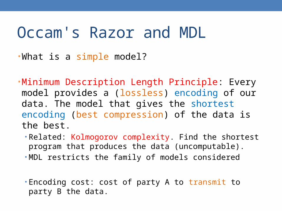
Occam's Razor and MDL
• What is a simple model?
• Minimum Description Length Principle: Every model provides a (lossless) encoding of our data. The model that gives the shortest encoding (best compression) of the data is the best.• Related: Kolmogorov complexity. Find the shortest
program that produces the data (uncomputable). • MDL restricts the family of models considered
• Encoding cost: cost of party A to transmit to party B the data.
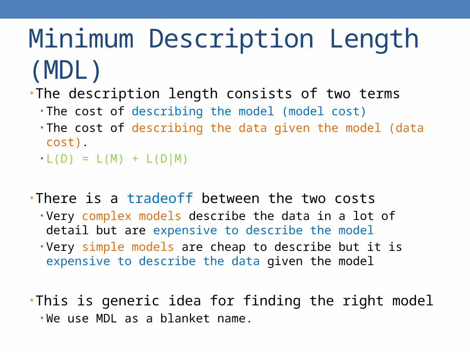
Minimum Description Length (MDL)• The description length consists of two terms
• The cost of describing the model (model cost)• The cost of describing the data given the model (data cost).• L(D) = L(M) + L(D|M)
• There is a tradeoff between the two costs• Very complex models describe the data in a lot of detail but are
expensive to describe the model• Very simple models are cheap to describe but it is expensive to
describe the data given the model
• This is generic idea for finding the right model• We use MDL as a blanket name.

6
Example• Regression: find a polynomial for describing a set of values
• Model complexity (model cost): polynomial coefficients• Goodness of fit (data cost): difference between real value and the polynomial
value
Source: Grunwald et al. (2005) Tutorial on MDL.
Minimum model costHigh data cost
High model costMinimum data cost
Low model costLow data cost
MDL avoids overfitting automatically!

Example • Suppose you want to describe a set of integer numbers
• Cost of describing a single number is proportional to the value of the number x (e.g., logx).
• How can we get an efficient description?
• Cluster integers into two clusters and describe the cluster by the centroid and the points by their distance from the centroid• Model cost: cost of the centroids• Data cost: cost of cluster membership and distance from centroid
• What are the two extreme cases?

MDL and Data Mining
• Why does the shorter encoding make sense?• Shorter encoding implies regularities in the data• Regularities in the data imply patterns• Patterns are interesting
• Example
00001000010000100001000010000100001000010001000010000100001
• Short description length, just repeat 12 times 00001
0100111001010011011010100001110101111011011010101110010011100
• Random sequence, no patterns, no compression

Is everything about compression?• Jürgen Schmidhuber:
A theory about creativity, art and fun• Interesting Art corresponds to a novel pattern that we cannot
compress well, yet it is not too random so we can learn it• Good Humor corresponds to an input that does not
compress well because it is out of place and surprising• Scientific discovery corresponds to a significant
compression event• E.g., a law that can explain all falling apples.
• Fun lecture:• Compression Progress: The Algorithmic Principle Behind Cu
riosity and Creativity

Issues with MDL
• What is the right model family?• This determines the kind of solutions that we can have
• E.g., polynomials • Clusterings
• What is the encoding cost?• Determines the function that we optimize• Information theory

INFORMATION THEORYA short introduction
Encoding
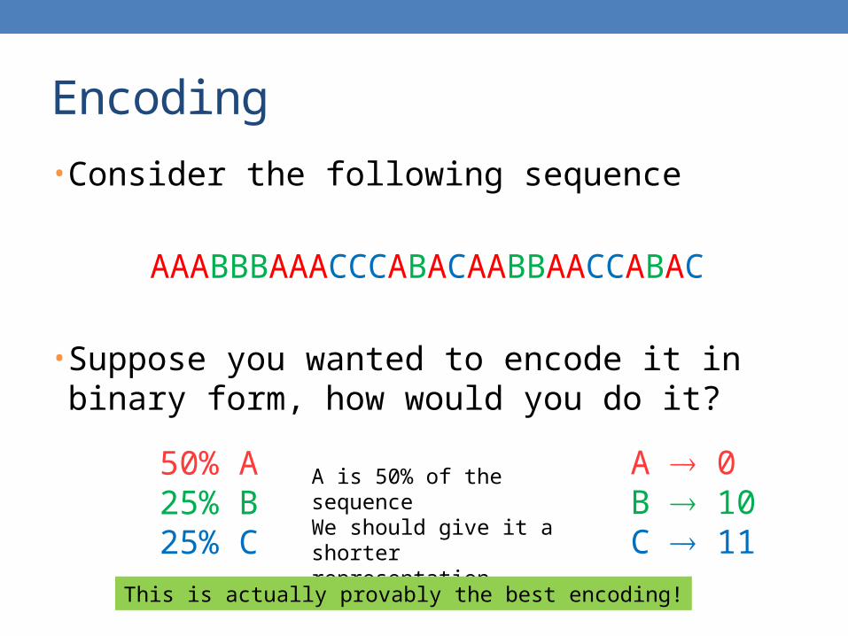
• Consider the following sequence
AAABBBAAACCCABACAABBAACCABAC
• Suppose you wanted to encode it in binary form, how would you do it?
A 0B 10C 11
A is 50% of the sequenceWe should give it a shorter representation
50% A 25% B 25% C
This is actually provably the best encoding!
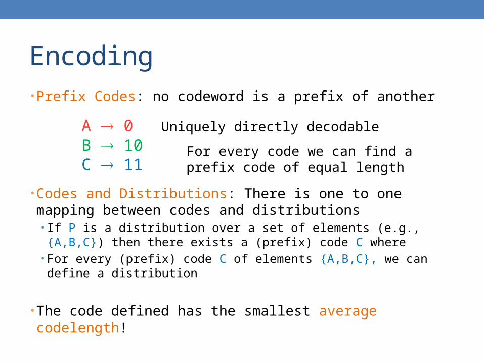
Encoding• Prefix Codes: no codeword is a prefix of another
• Codes and Distributions: There is one to one mapping between codes and distributions• If P is a distribution over a set of elements (e.g., {A,B,C}) then
there exists a (prefix) code C where • For every (prefix) code C of elements {A,B,C}, we can define a
distribution
• The code defined has the smallest average codelength!
A 0B 10C 11
Uniquely directly decodable
For every code we can find a prefix code of equal length

Entropy• Suppose we have a random variable X that takes n distinct values
that have probabilities
• This defines a code C with . The average codelength is
• This (more or less) is the entropy of the random variable X
• Shannon’s theorem: The entropy is a lower bound on the average codelength of any code that encodes the distribution P(X)• When encoding N numbers drawn from P(X), the best encoding length we
can hope for is • Reminder: Lossless encoding
Entropy
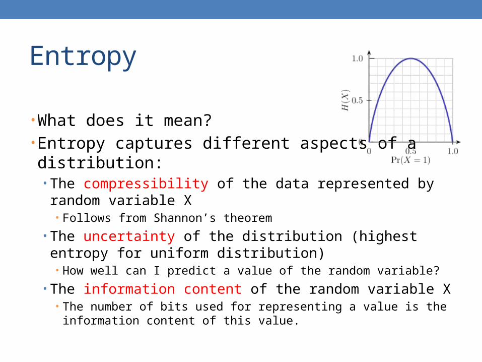
• What does it mean?• Entropy captures different aspects of a distribution:
• The compressibility of the data represented by random variable X• Follows from Shannon’s theorem
• The uncertainty of the distribution (highest entropy for uniform distribution)• How well can I predict a value of the random variable?
• The information content of the random variable X• The number of bits used for representing a value is the
information content of this value.
Claude Shannon
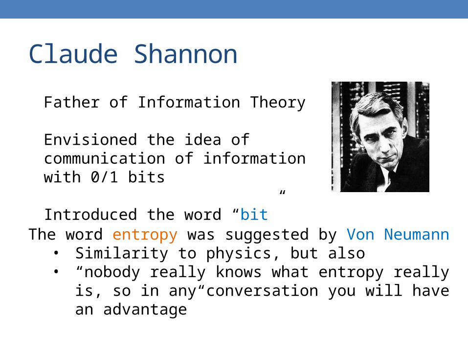
Father of Information Theory
Envisioned the idea of communication of information with 0/1 bits
Introduced the word “bit”
The word entropy was suggested by Von Neumann• Similarity to physics, but also • “nobody really knows what entropy really is, so in any
conversation you will have an advantage”

Some information theoretic measures
• Conditional entropy H(Y|X): the uncertainty for Y given that we know X
• Mutual Information I(X,Y): The reduction in the uncertainty for Y (or X) given that we know X (or Y)

Some information theoretic measures
• Cross Entropy: The cost of encoding distribution P, using the code of distribution Q
• KL Divergence KL(P||Q): The increase in encoding cost for distribution P when using the code of distribution Q
• Not symmetric• Problematic if Q not defined for all x of P.
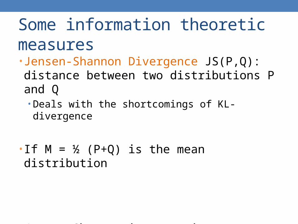
Some information theoretic measures
• Jensen-Shannon Divergence JS(P,Q): distance between two distributions P and Q• Deals with the shortcomings of KL-divergence
• If M = ½ (P+Q) is the mean distribution
• Jensen-Shannon is a metric

USING MDL FOR CO-CLUSTERING(CROSS-ASSOCIATIONS)
Thanks to Spiros Papadimitriou.

Co-clustering
• Simultaneous grouping of rows and columns of a matrix into homogeneous groups
5 10 15 20 25
5
10
15
20
25
97%
96%
3%
3%
Product groups
Cus
tom
er g
rou
ps
5 10 15 20 25
5
10
15
20
25
Products
54%
Cus
tom
ers
Students buying books
CEOs buying BMWs

Co-clustering
• Step 1: How to define a “good” partitioning?
Intuition and formalization
• Step 2: How to find it?

Co-clusteringIntuition
versus
Column groups Column groups
Row
gro
ups
Row
gro
ups
Good Clustering
1. Similar nodes are grouped together
2. As few groups as necessary
A few, homogeneous blocks
Good Compression
Why is this better?
implies
log*k + log*ℓ log nimj
i,j nimj H(pi,j)
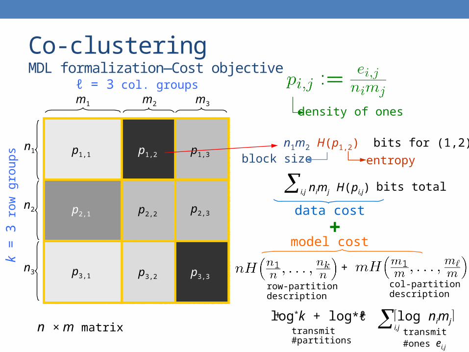
Co-clusteringMDL formalization—Cost objective
n1
n2
n3
m1 m2 m3
p1,1 p1,2 p1,3
p2,1 p2,2 p2,3
p3,3p3,2p3,1
n × m matrix
k =
3 r
ow g
roup
s
ℓ = 3 col. groups
density of ones
n1m2 H(p1,2) bits for (1,2)
data cost
bits total
row-partitiondescription
col-partitiondescription
i,jtransmit#ones ei,j
+
+
model cost+
block size entropy
+transmit#partitions

Co-clusteringMDL formalization—Cost objective
code cost(block contents)
description cost(block structure)
+
one row groupone col group
n row groupsm col groups
low
high low
high

Co-clusteringMDL formalization—Cost objective
code cost(block contents)
description cost(block structure)
+
k = 3 row groupsℓ = 3 col groups
low
low
Co-clusteringMDL formalization—Cost objective
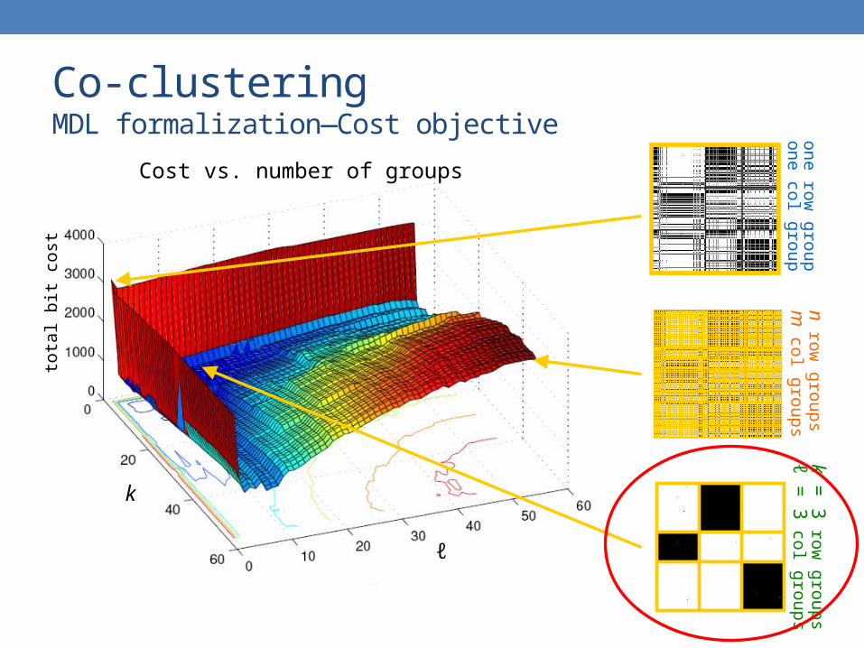
k
ℓ
tota
l bit
cost
Cost vs. number of groups
one row
groupone
col group
n row
groupsm
col g
roupsk =
3 row
groupsℓ =
3 co
l groups

Co-clustering
• Step 1: How to define a “good” partitioning?
Intuition and formalization
• Step 2: How to find it?

Search for solutionOverview: assignments w/ fixed number of groups (shuffles)
row shuffle column shuffle row shuffleoriginal groups
No cost improvement:Discard
reassign all rows,holding columnassignments fixed
reassign all columns,holding rowassignments fixed

Search for solutionOverview: assignments w/ fixed number of groups (shuffles)
row shuffle column shuffle column shuffle
row shufflecolumn shuffle
No cost improvement:Discard
Final shuffle result
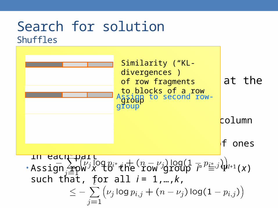
Search for solutionShuffles• Let
denote row and col. partitions at the I-th iteration• Fix I and for every row x:
• Splice into ℓ parts, one for each column group• Let j, for j = 1,…,ℓ, be the number of ones in each part• Assign row x to the row group i¤ I+1(x) such that, for all i
= 1,…,k,
p1,1 p1,2 p1,3
p2,1 p2,2 p2,3
p3,3p3,2p3,1
Similarity (“KL-divergences”)of row fragmentsto blocks of a row group
Assign to second row-group
k = 5, ℓ = 5
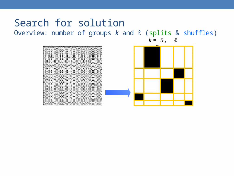
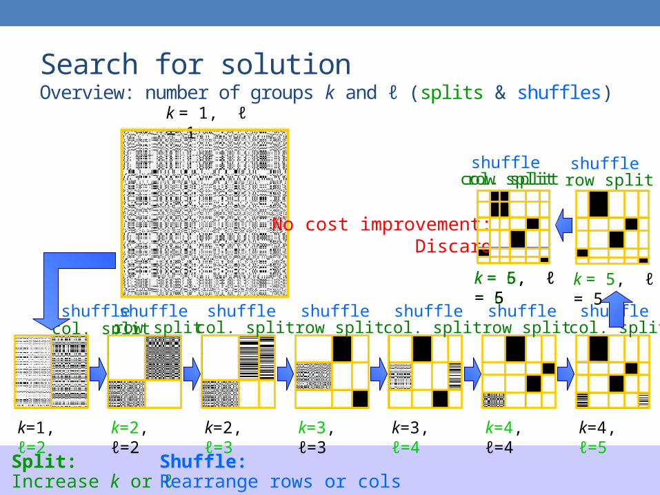
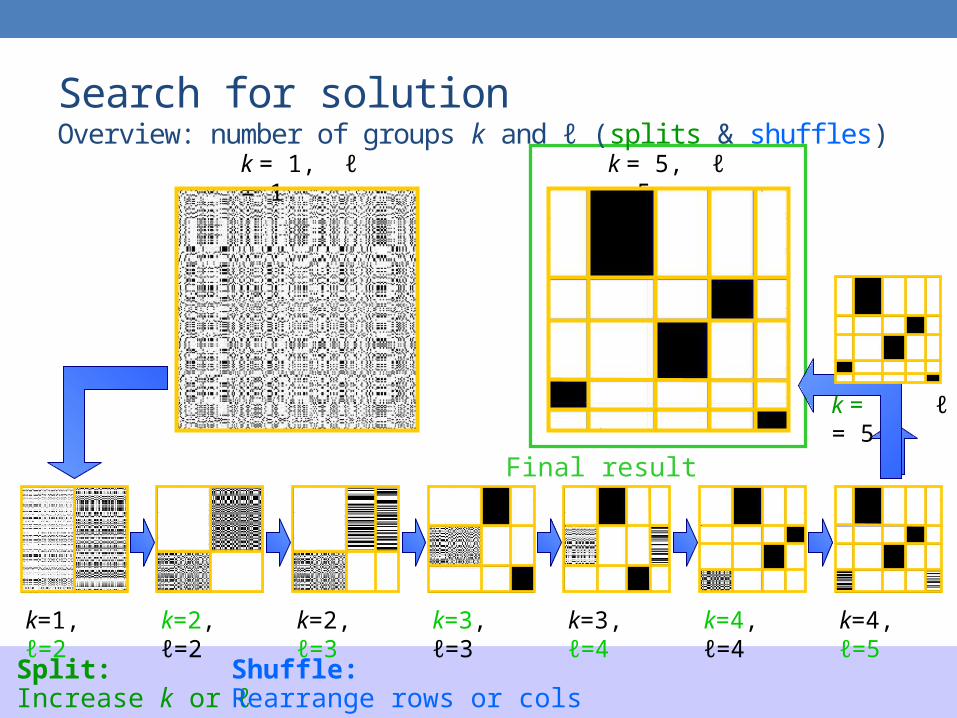
Search for solutionOverview: number of groups k and ℓ (splits & shuffles)
col. splitshuffle
Search for solutionOverview: number of groups k and ℓ (splits & shuffles)
k=1, ℓ=2 k=2, ℓ=2 k=2, ℓ=3 k=3, ℓ=3 k=3, ℓ=4 k=4, ℓ=4 k=4, ℓ=5
k = 1, ℓ = 1
row splitshuffle
Split:Increase k or ℓ
Shuffle:Rearrange rows or cols
col. splitshuffle
row splitshuffle
col. splitshuffle
row splitshuffle
col. splitshuffle
k = 5, ℓ = 5
row splitshuffle
k = 5, ℓ = 6
col. splitshuffle
No cost improvement:Discard
row split
k = 6, ℓ = 5
Search for solutionOverview: number of groups k and ℓ (splits & shuffles)
k=1, ℓ=2 k=2, ℓ=2 k=2, ℓ=3 k=3, ℓ=3 k=3, ℓ=4 k=4, ℓ=4 k=4, ℓ=5
k = 1, ℓ = 1
Split:Increase k or ℓ
Shuffle:Rearrange rows or cols
k = 5, ℓ = 5
k = 5, ℓ = 5
Final result

Co-clusteringCLASSIC
CLASSIC corpus• 3,893 documents• 4,303 words• 176,347 “dots” (edges)
Combination of 3 sources:• MEDLINE (medical)• CISI (info. retrieval)• CRANFIELD (aerodynamics)
Doc
umen
ts
Words

Graph co-clusteringCLASSIC
Doc
umen
ts
Words
“CLASSIC” graph of documents & words: k = 15, ℓ = 19

Co-clusteringCLASSIC
MEDLINE(medical)
insipidus, alveolar, aortic, death, prognosis, intravenous
blood, disease, clinical, cell, tissue, patient
“CLASSIC” graph of documents & words: k = 15, ℓ = 19
CISI(Information Retrieval)
providing, studying, records, development, students, rules
abstract, notation, works, construct, bibliographies
shape, nasa, leading, assumed, thin
paint, examination, fall, raise, leave, based
CRANFIELD (aerodynamics)

Co-clusteringCLASSIC
Document cluster #
Document class Precision
CRANFIELD CISI MEDLINE
1 0 1 390 0.9972 0 0 610 1.0003 2 676 9 0.9844 1 317 6 0.9785 3 452 16 0.9606 207 0 0 1.0007 188 0 0 1.0008 131 0 0 1.0009 209 0 0 1.000
10 107 2 0 0.98211 152 3 2 0.96812 74 0 0 1.00013 139 9 0 0.93914 163 0 0 1.00015 24 0 0 1.000
Recall 0.996 0.990 0.968
0.94
-1.0
0
0.97-0.99
0.999
0.975
0.987
Related Documents