Data Mining K-means Algorithm 1

Welcome message from author
This document is posted to help you gain knowledge. Please leave a comment to let me know what you think about it! Share it to your friends and learn new things together.
Transcript
Data MiningK-means Algorithm
1

© Tan,Steinbach, Kumar Introduction to Data Mining 4/18/2004 2
What is Cluster Analysis?
Finding groups of objects such that the objects in a group will be similar (or related) to one another and different from (or unrelated to) the objects in other groups
Inter-cluster distances are maximized
Intra-cluster distances are
minimized

© Tan,Steinbach, Kumar Introduction to Data Mining 4/18/2004 3
Applications of Cluster Analysis
Understanding– Group related documents
for browsing, group genes and proteins that have similar functionality, or group stocks with similar price fluctuations
Summarization– Reduce the size of large
data sets
Clustering precipitation in Australia
© Tan,Steinbach, Kumar Introduction to Data Mining 4/18/2004 4
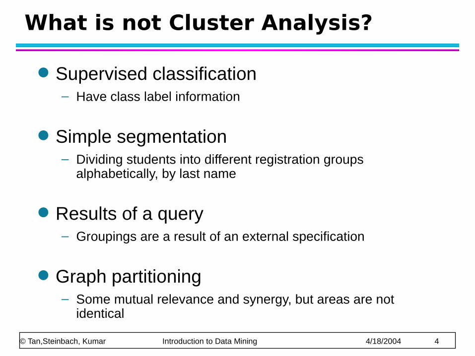
What is not Cluster Analysis?
Supervised classification– Have class label information
Simple segmentation– Dividing students into different registration groups
alphabetically, by last name
Results of a query– Groupings are a result of an external specification
Graph partitioning– Some mutual relevance and synergy, but areas are not
identical

© Tan,Steinbach, Kumar Introduction to Data Mining 4/18/2004 5
Notion of a Cluster can be Ambiguous
How many clusters?
Four Clusters Two Clusters
Six Clusters

© Tan,Steinbach, Kumar Introduction to Data Mining 4/18/2004 6
Types of Clusterings
A clustering is a set of clusters
Important distinction between hierarchical and partitional sets of clusters
Partitional Clustering– A division data objects into non-overlapping subsets (clusters)
such that each data object is in exactly one subset
Hierarchical clustering– A set of nested clusters organized as a hierarchical tree

© Tan,Steinbach, Kumar Introduction to Data Mining 4/18/2004 7
Partitional Clustering
Original Points A Partitional Clustering
© Tan,Steinbach, Kumar Introduction to Data Mining 4/18/2004 8
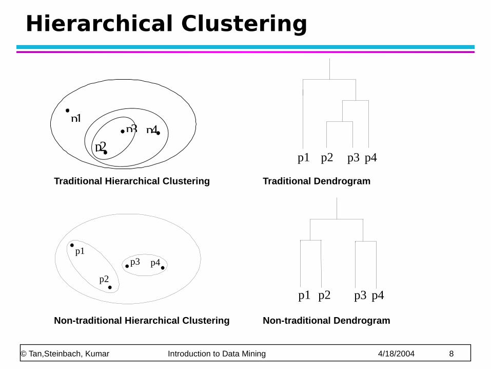
Hierarchical Clustering
p4p1
p3
p2
p4 p1
p3 p2
p4p1 p2 p3
p4p1 p2 p3
Traditional Hierarchical Clustering
Non-traditional Hierarchical Clustering Non-traditional Dendrogram
Traditional Dendrogram

© Tan,Steinbach, Kumar Introduction to Data Mining 4/18/2004 9
Other Distinctions Between Sets of Clusters
Exclusive versus non-exclusive– In non-exclusive clusterings, points may belong to multiple
clusters.– Can represent multiple classes or ‘border’ points
Fuzzy versus non-fuzzy– In fuzzy clustering, a point belongs to every cluster with some
weight between 0 and 1– Weights must sum to 1– Probabilistic clustering has similar characteristics
Partial versus complete– In some cases, we only want to cluster some of the data
Heterogeneous versus homogeneous– Cluster of widely different sizes, shapes, and densities
© Tan,Steinbach, Kumar Introduction to Data Mining 4/18/2004 10
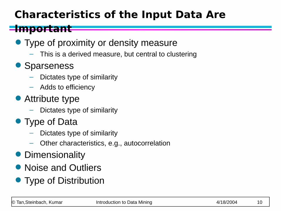
Characteristics of the Input Data Are Important Type of proximity or density measure
– This is a derived measure, but central to clustering
Sparseness– Dictates type of similarity– Adds to efficiency
Attribute type– Dictates type of similarity
Type of Data– Dictates type of similarity– Other characteristics, e.g., autocorrelation
Dimensionality Noise and Outliers Type of Distribution

© Tan,Steinbach, Kumar Introduction to Data Mining 4/18/2004 11
K-means Clustering
Partitional clustering approach Each cluster is associated with a centroid (center point) Each point is assigned to the cluster with the closest centroid Number of clusters, K, must be specified The basic algorithm is very simple

© Tan,Steinbach, Kumar Introduction to Data Mining 4/18/2004 12
K-means Clustering – Details Initial centroids are often chosen randomly.
– Clusters produced vary from one run to another.
The centroid is (typically) the mean of the points in the cluster. ‘Closeness’ is measured by Euclidean distance, cosine similarity, correlation, etc. K-means will converge for common similarity measures mentioned above. Most of the convergence happens in the first few iterations.
– Often the stopping condition is changed to ‘Until relatively few points change clusters’
Complexity is O( n * K * I * d )– n = number of points, K = number of clusters,
I = number of iterations, d = number of attributes

© Tan,Steinbach, Kumar Introduction to Data Mining 4/18/2004 13
Two different K-means Clusterings
2 1.5 1 0.5 0 0.5 1 1.5 2
0
0.5
1
1.5
2
2.5
3
x
y
2 1.5 1 0.5 0 0.5 1 1.5 2
0
0.5
1
1.5
2
2.5
3
x
y
Sub-optimal Clustering
2 1.5 1 0.5 0 0.5 1 1.5 2
0
0.5
1
1.5
2
2.5
3
x
y
Optimal Clustering
Original Points

© Tan,Steinbach, Kumar Introduction to Data Mining 4/18/2004 14
Importance of Choosing Initial Centroids
2 1.5 1 0.5 0 0.5 1 1.5 2
0
0.5
1
1.5
2
2.5
3
x
y
Iteration 1
2 1.5 1 0.5 0 0.5 1 1.5 2
0
0.5
1
1.5
2
2.5
3
x
y
Iteration 2
2 1.5 1 0.5 0 0.5 1 1.5 2
0
0.5
1
1.5
2
2.5
3
x
y
Iteration 3
2 1.5 1 0.5 0 0.5 1 1.5 2
0
0.5
1
1.5
2
2.5
3
x
y
Iteration 4
2 1.5 1 0.5 0 0.5 1 1.5 2
0
0.5
1
1.5
2
2.5
3
x
y
Iteration 5
2 1.5 1 0.5 0 0.5 1 1.5 2
0
0.5
1
1.5
2
2.5
3
x
y
Iteration 6

© Tan,Steinbach, Kumar Introduction to Data Mining 4/18/2004 15
Importance of Choosing Initial Centroids
2 1.5 1 0.5 0 0.5 1 1.5 2
0
0.5
1
1.5
2
2.5
3
x
y
Iteration 1
2 1.5 1 0.5 0 0.5 1 1.5 2
0
0.5
1
1.5
2
2.5
3
x
y
Iteration 2
2 1.5 1 0.5 0 0.5 1 1.5 2
0
0.5
1
1.5
2
2.5
3
x
y
Iteration 3
2 1.5 1 0.5 0 0.5 1 1.5 2
0
0.5
1
1.5
2
2.5
3
x
y
Iteration 4
2 1.5 1 0.5 0 0.5 1 1.5 2
0
0.5
1
1.5
2
2.5
3
x
y
Iteration 5
2 1.5 1 0.5 0 0.5 1 1.5 2
0
0.5
1
1.5
2
2.5
3
x
y
Iteration 6

© Tan,Steinbach, Kumar Introduction to Data Mining 4/18/2004 16
Evaluating K-means Clusters
Most common measure is Sum of Squared Error (SSE)– For each point, the error is the distance to the nearest cluster– To get SSE, we square these errors and sum them.
– x is a data point in cluster Ci and mi is the representative point for cluster Ci can show that mi corresponds to the center (mean) of the cluster
– Given two clusters, we can choose the one with the smallest error
– One easy way to reduce SSE is to increase K, the number of clusters A good clustering with smaller K can have a lower SSE than a poor clustering with higher K
K
i Cxi
i
xmdistSSE1
2 ),(

© Tan,Steinbach, Kumar Introduction to Data Mining 4/18/2004 17
Importance of Choosing Initial Centroids …
2 1.5 1 0.5 0 0.5 1 1.5 2
0
0.5
1
1.5
2
2.5
3
x
y
Iteration 1
2 1.5 1 0.5 0 0.5 1 1.5 2
0
0.5
1
1.5
2
2.5
3
x
y
Iteration 2
2 1.5 1 0.5 0 0.5 1 1.5 2
0
0.5
1
1.5
2
2.5
3
x
y
Iteration 3
2 1.5 1 0.5 0 0.5 1 1.5 2
0
0.5
1
1.5
2
2.5
3
x
y
Iteration 4
2 1.5 1 0.5 0 0.5 1 1.5 2
0
0.5
1
1.5
2
2.5
3
x
y
Iteration 5

© Tan,Steinbach, Kumar Introduction to Data Mining 4/18/2004 18
Importance of Choosing Initial Centroids …
2 1.5 1 0.5 0 0.5 1 1.5 2
0
0.5
1
1.5
2
2.5
3
x
y
Iteration 1
2 1.5 1 0.5 0 0.5 1 1.5 2
0
0.5
1
1.5
2
2.5
3
x
y
Iteration 2
2 1.5 1 0.5 0 0.5 1 1.5 2
0
0.5
1
1.5
2
2.5
3
x
y
Iteration 3
2 1.5 1 0.5 0 0.5 1 1.5 2
0
0.5
1
1.5
2
2.5
3
x
y
Iteration 4
2 1.5 1 0.5 0 0.5 1 1.5 2
0
0.5
1
1.5
2
2.5
3
xy
Iteration 5

© Tan,Steinbach, Kumar Introduction to Data Mining 4/18/2004 19
Problems with Selecting Initial Points
If there are K ‘real’ clusters then the chance of selecting one centroid from each cluster is small. – Chance is relatively small when K is large
– If clusters are the same size, n, then
– For example, if K = 10, then probability = 10!/1010 = 0.00036
– Sometimes the initial centroids will readjust themselves in ‘right’ way, and sometimes they don’t
– Consider an example of five pairs of clusters

© Tan,Steinbach, Kumar Introduction to Data Mining 4/18/2004 20
10 Clusters Example
0 5 10 15 20
6
4
2
0
2
4
6
8
x
yIteration 1
0 5 10 15 20
6
4
2
0
2
4
6
8
x
yIteration 2
0 5 10 15 20
6
4
2
0
2
4
6
8
x
yIteration 3
0 5 10 15 20
6
4
2
0
2
4
6
8
x
yIteration 4
Starting with two initial centroids in one cluster of each pair of clusters

© Tan,Steinbach, Kumar Introduction to Data Mining 4/18/2004 21
10 Clusters Example
0 5 10 15 20
6
4
2
0
2
4
6
8
x
y
Iteration 1
0 5 10 15 20
6
4
2
0
2
4
6
8
x
y
Iteration 2
0 5 10 15 20
6
4
2
0
2
4
6
8
x
y
Iteration 3
0 5 10 15 20
6
4
2
0
2
4
6
8
x
y
Iteration 4
Starting with two initial centroids in one cluster of each pair of clusters

© Tan,Steinbach, Kumar Introduction to Data Mining 4/18/2004 22
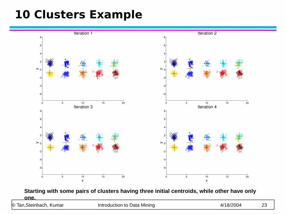
10 Clusters Example
Starting with some pairs of clusters having three initial centroids, while other have only one.
0 5 10 15 20
6
4
2
0
2
4
6
8
x
y
Iteration 1
0 5 10 15 20
6
4
2
0
2
4
6
8
x
y
Iteration 2
0 5 10 15 20
6
4
2
0
2
4
6
8
x
y
Iteration 3
0 5 10 15 20
6
4
2
0
2
4
6
8
x
y
Iteration 4
© Tan,Steinbach, Kumar Introduction to Data Mining 4/18/2004 23
10 Clusters Example
Starting with some pairs of clusters having three initial centroids, while other have only one.
0 5 10 15 20
6
4
2
0
2
4
6
8
x
yIteration 1
0 5 10 15 20
6
4
2
0
2
4
6
8
x
y
Iteration 2
0 5 10 15 20
6
4
2
0
2
4
6
8
x
y
Iteration 3
0 5 10 15 20
6
4
2
0
2
4
6
8
x
y
Iteration 4
© Tan,Steinbach, Kumar Introduction to Data Mining 4/18/2004 24
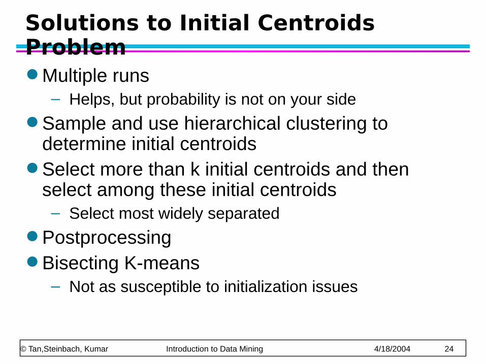
Solutions to Initial Centroids Problem Multiple runs
– Helps, but probability is not on your side Sample and use hierarchical clustering to
determine initial centroids Select more than k initial centroids and then
select among these initial centroids– Select most widely separated
Postprocessing Bisecting K-means
– Not as susceptible to initialization issues

© Tan,Steinbach, Kumar Introduction to Data Mining 4/18/2004 25
Handling Empty Clusters
Basic K-means algorithm can yield empty clusters
Several strategies– Choose the point that contributes most to SSE
– Choose a point from the cluster with the highest SSE
– If there are several empty clusters, the above can be repeated several times.

© Tan,Steinbach, Kumar Introduction to Data Mining 4/18/2004 26
Updating Centers Incrementally
In the basic K-means algorithm, centroids are updated after all points are assigned to a centroid
An alternative is to update the centroids after each assignment (incremental approach)– Each assignment updates zero or two centroids
– More expensive
– Introduces an order dependency
– Never get an empty cluster
– Can use “weights” to change the impact

© Tan,Steinbach, Kumar Introduction to Data Mining 4/18/2004 27
Pre-processing and Post-processing Pre-processing
– Normalize the data
– Eliminate outliers
Post-processing– Eliminate small clusters that may represent outliers
– Split ‘loose’ clusters, i.e., clusters with relatively high SSE
– Merge clusters that are ‘close’ and that have relatively low SSE
– Can use these steps during the clustering process ISODATA

© Tan,Steinbach, Kumar Introduction to Data Mining 4/18/2004 28
Bisecting K-means
Bisecting K-means algorithm– Variant of K-means that can produce a partitional or a hierarchical clustering

© Tan,Steinbach, Kumar Introduction to Data Mining 4/18/2004 29
Bisecting K-means Example

© Tan,Steinbach, Kumar Introduction to Data Mining 4/18/2004 30
Limitations of K-means
K-means has problems when clusters are of differing – Sizes
– Densities
– Non-globular shapes
K-means has problems when the data contains outliers.

© Tan,Steinbach, Kumar Introduction to Data Mining 4/18/2004 31
Limitations of K-means: Differing Sizes
Original Points K-means (3 Clusters)

© Tan,Steinbach, Kumar Introduction to Data Mining 4/18/2004 32
Limitations of K-means: Differing Density
Original Points K-means (3 Clusters)

© Tan,Steinbach, Kumar Introduction to Data Mining 4/18/2004 33
Limitations of K-means: Non-globular Shapes
Original Points K-means (2 Clusters)
© Tan,Steinbach, Kumar Introduction to Data Mining 4/18/2004 34
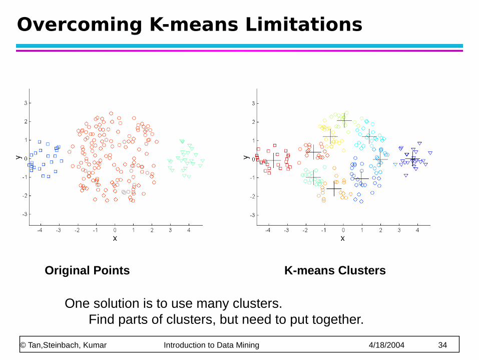
Overcoming K-means Limitations
Original Points K-means Clusters
One solution is to use many clusters.Find parts of clusters, but need to put together.
© Tan,Steinbach, Kumar Introduction to Data Mining 4/18/2004 35
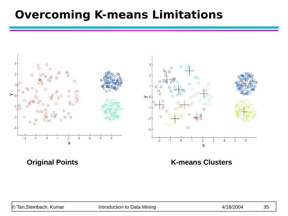
Overcoming K-means Limitations
Original Points K-means Clusters

© Tan,Steinbach, Kumar Introduction to Data Mining 4/18/2004 36
Overcoming K-means Limitations
Original Points K-means Clusters
Related Documents