Classification: Alternative Techniques Lecture Notes for Chapter 5 Introduction to Data Mining by Tan, Steinbach, Kumar © Tan,Steinbach, Kumar Introduction to Data Mining 4/18/2004 1

Data Mining Classification: Alternative Techniques Lecture Notes for Chapter 5 Introduction to Data Mining by Tan, Steinbach, Kumar © Tan,Steinbach, Kumar.
Dec 15, 2015
Welcome message from author
This document is posted to help you gain knowledge. Please leave a comment to let me know what you think about it! Share it to your friends and learn new things together.
Transcript
Data Mining Classification: Alternative
Techniques
Lecture Notes for Chapter 5
Introduction to Data Miningby
Tan, Steinbach, Kumar
© Tan,Steinbach, Kumar Introduction to Data Mining 4/18/2004 1

© Tan,Steinbach, Kumar Introduction to Data Mining 4/18/2004 2
Rule Based Method: See new lecture notes
© Tan,Steinbach, Kumar Introduction to Data Mining 4/18/2004 3
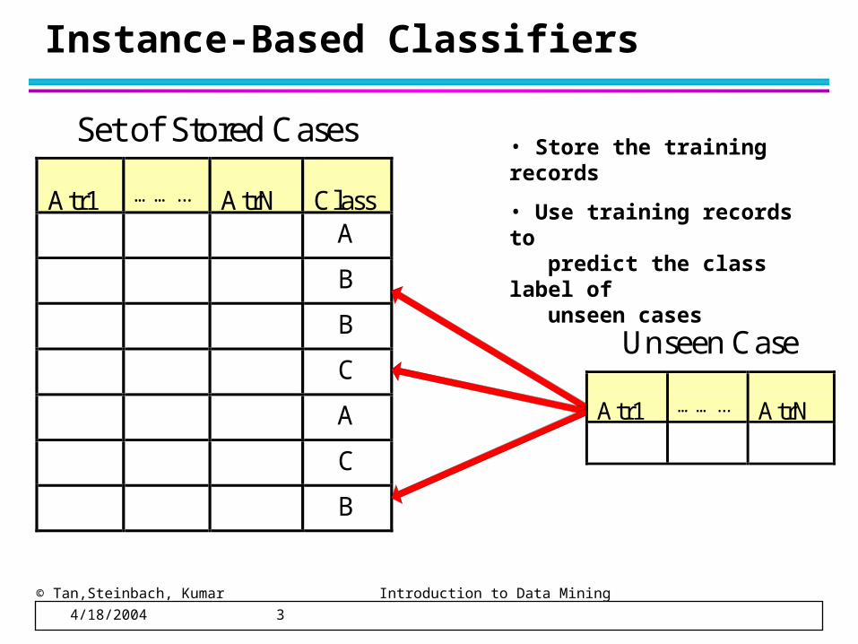
Instance-Based Classifiers
Atr1 ……... AtrN ClassA
B
B
C
A
C
B
Set of Stored Cases
Atr1 ……... AtrN
Unseen Case
• Store the training records
• Use training records to predict the class label of unseen cases
© Tan,Steinbach, Kumar Introduction to Data Mining 4/18/2004 4
Instance Based Classifiers
Examples:
– Rote-learner Memorizes entire training data and performs classification only if attributes of record match one of the training examples exactly
– Nearest neighbor Uses k “closest” points (nearest neighbors) for performing classification
© Tan,Steinbach, Kumar Introduction to Data Mining 4/18/2004 5
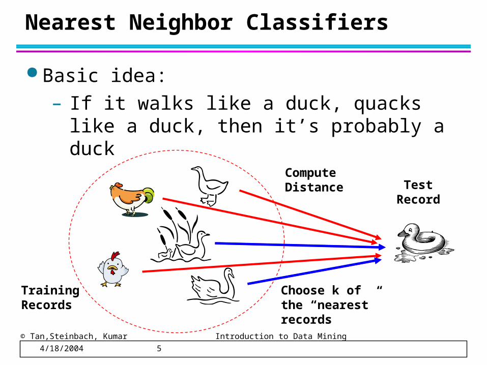
Nearest Neighbor Classifiers
Basic idea:
– If it walks like a duck, quacks like a duck, then it’s probably a duck
Training Records
Test Record
Compute Distance
Choose k of the “nearest” records
© Tan,Steinbach, Kumar Introduction to Data Mining 4/18/2004 6
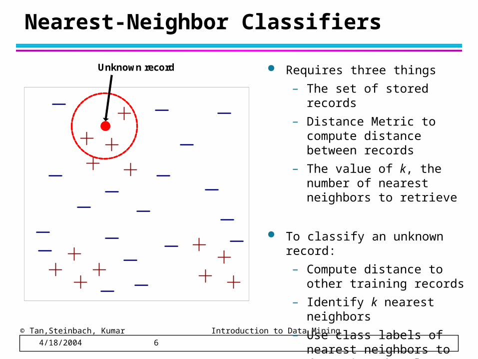
Nearest-Neighbor Classifiers
Requires three things
– The set of stored records
– Distance Metric to compute distance between records
– The value of k, the number of nearest neighbors to retrieve
To classify an unknown record:
– Compute distance to other training records
– Identify k nearest neighbors
– Use class labels of nearest neighbors to determine the class label of unknown record (e.g., by taking majority vote)
Unknown record
© Tan,Steinbach, Kumar Introduction to Data Mining 4/18/2004 7
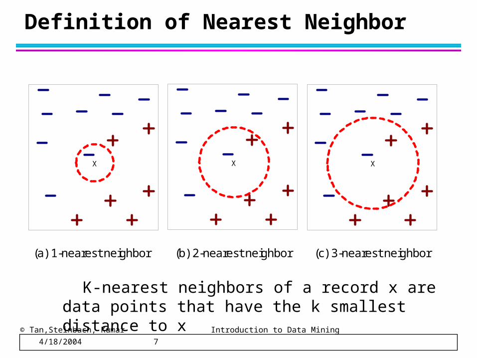
Definition of Nearest Neighbor
X X X
(a) 1-nearest neighbor (b) 2-nearest neighbor (c) 3-nearest neighbor
K-nearest neighbors of a record x are data points that have the k smallest distance to x
© Tan,Steinbach, Kumar Introduction to Data Mining 4/18/2004 8
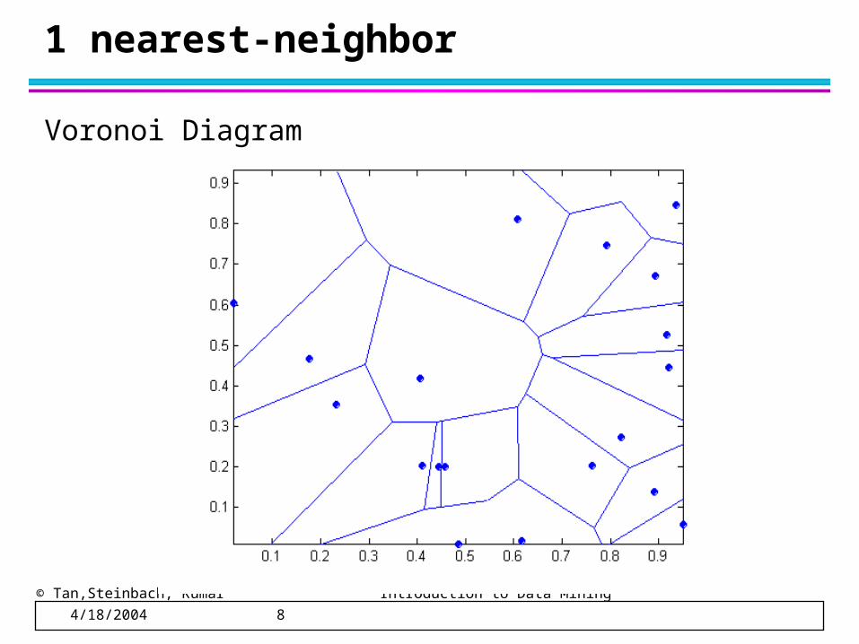
1 nearest-neighbor
Voronoi Diagram
© Tan,Steinbach, Kumar Introduction to Data Mining 4/18/2004 9
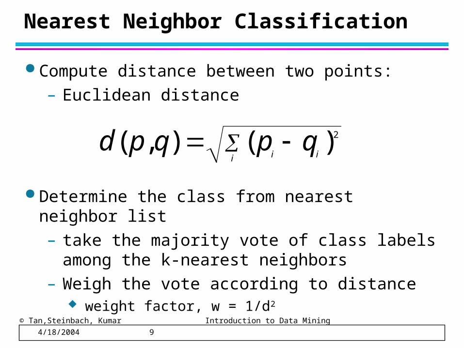
Nearest Neighbor Classification
Compute distance between two points:
– Euclidean distance
Determine the class from nearest neighbor list
– take the majority vote of class labels among the k-nearest neighbors
– Weigh the vote according to distance weight factor, w = 1/d2
i ii
qpqpd 2)(),(
© Tan,Steinbach, Kumar Introduction to Data Mining 4/18/2004 10
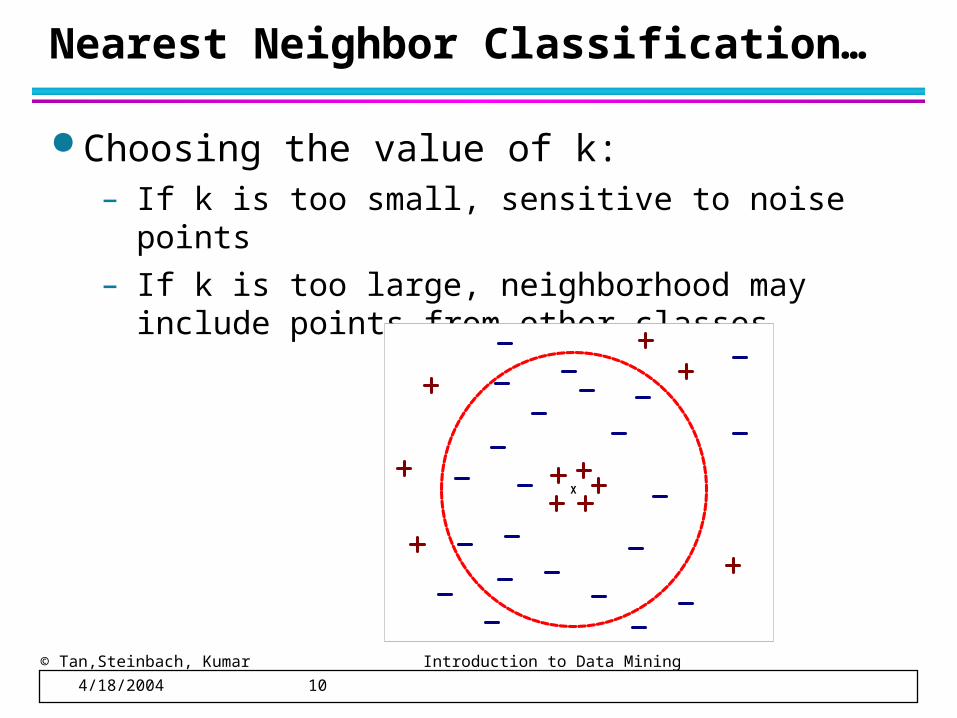
Nearest Neighbor Classification…
Choosing the value of k:– If k is too small, sensitive to noise points
– If k is too large, neighborhood may include points from other classes
X
© Tan,Steinbach, Kumar Introduction to Data Mining 4/18/2004 11
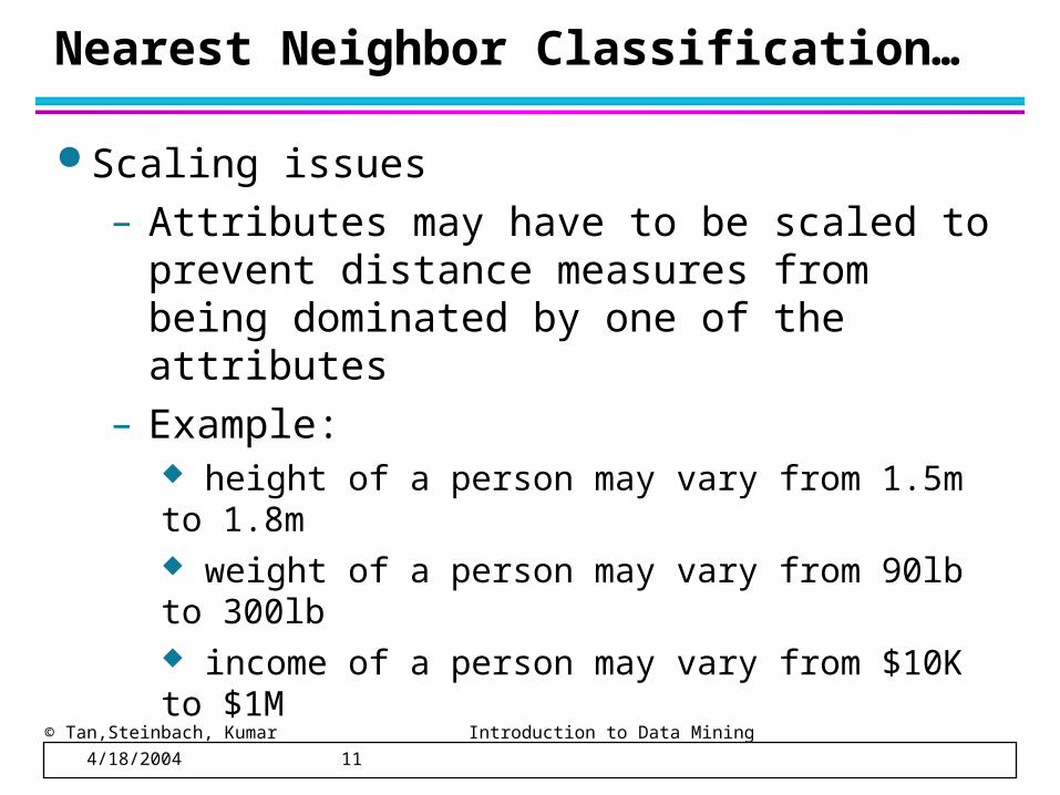
Nearest Neighbor Classification…
Scaling issues
– Attributes may have to be scaled to prevent distance measures from being dominated by one of the attributes
– Example: height of a person may vary from 1.5m to 1.8m weight of a person may vary from 90lb to 300lb income of a person may vary from $10K to $1M
© Tan,Steinbach, Kumar Introduction to Data Mining 4/18/2004 12
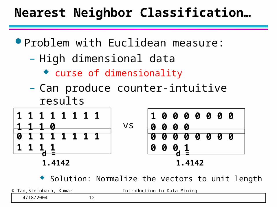
Nearest Neighbor Classification…
Problem with Euclidean measure:
– High dimensional data curse of dimensionality
– Can produce counter-intuitive results
1 1 1 1 1 1 1 1 1 1 1 0
0 1 1 1 1 1 1 1 1 1 1 1
1 0 0 0 0 0 0 0 0 0 0 0
0 0 0 0 0 0 0 0 0 0 0 1vs
d = 1.4142 d = 1.4142
Solution: Normalize the vectors to unit length
© Tan,Steinbach, Kumar Introduction to Data Mining 4/18/2004 13
Nearest neighbor Classification…
k-NN classifiers are lazy learners
– It does not build models explicitly
– Unlike eager learners such as decision tree induction and rule-based systems
– Classifying unknown records are relatively expensive
© Tan,Steinbach, Kumar Introduction to Data Mining 4/18/2004 14
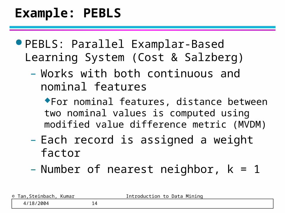
Example: PEBLS
PEBLS: Parallel Examplar-Based Learning System (Cost & Salzberg)
– Works with both continuous and nominal featuresFor nominal features, distance between two nominal values is computed using modified value difference metric (MVDM)
– Each record is assigned a weight factor
– Number of nearest neighbor, k = 1
© Tan,Steinbach, Kumar Introduction to Data Mining 4/18/2004 15
Example: PEBLS
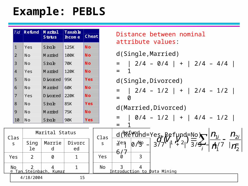
ClassMarital Status
Single Married Divorced
Yes 2 0 1
No 2 4 1
i
ii
n
n
n
nVVd
2
2
1
121 ),(
Distance between nominal attribute values:
d(Single,Married)
= | 2/4 – 0/4 | + | 2/4 – 4/4 | = 1
d(Single,Divorced)
= | 2/4 – 1/2 | + | 2/4 – 1/2 | = 0
d(Married,Divorced)
= | 0/4 – 1/2 | + | 4/4 – 1/2 | = 1
d(Refund=Yes,Refund=No)
= | 0/3 – 3/7 | + | 3/3 – 4/7 | = 6/7
Tid Refund MaritalStatus
TaxableIncome Cheat
1 Yes Single 125K No
2 No Married 100K No
3 No Single 70K No
4 Yes Married 120K No
5 No Divorced 95K Yes
6 No Married 60K No
7 Yes Divorced 220K No
8 No Single 85K Yes
9 No Married 75K No
10 No Single 90K Yes10
ClassRefund
Yes No
Yes 0 3
No 3 4
© Tan,Steinbach, Kumar Introduction to Data Mining 4/18/2004 16
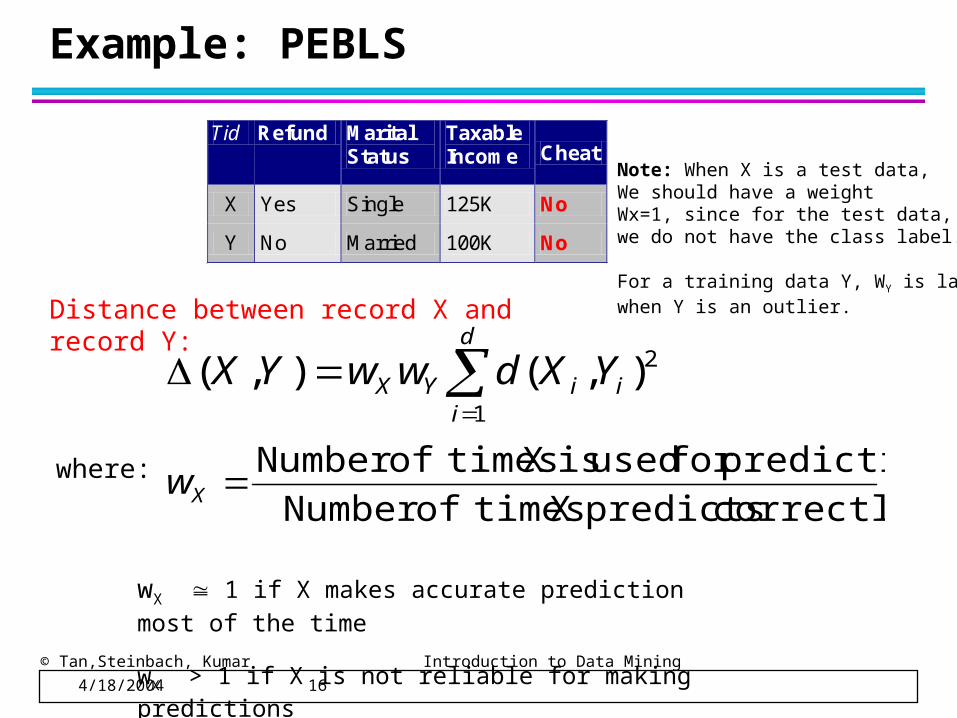
Example: PEBLS
d
iiiYX YXdwwYX
1
2),(),(
Tid Refund Marital Status
Taxable Income Cheat
X Yes Single 125K No
Y No Married 100K No 10
Distance between record X and record Y:
where:
correctly predicts X timesofNumber
predictionfor used is X timesofNumber Xw
wX 1 if X makes accurate prediction most of the time
wX > 1 if X is not reliable for making predictions
Note: When X is a test data,We should have a weightWx=1, since for the test data,we do not have the class label.
For a training data Y, WY is largewhen Y is an outlier.

© Tan,Steinbach, Kumar Introduction to Data Mining 4/18/2004 17
Bayes Classifier
A probabilistic framework for solving classification problems
Conditional Probability:
Bayes theorem:
)()()|(
)|(AP
CPCAPACP
)(),(
)|(
)(),(
)|(
CPCAP
CAP
APCAP
ACP
© Tan,Steinbach, Kumar Introduction to Data Mining 4/18/2004 18
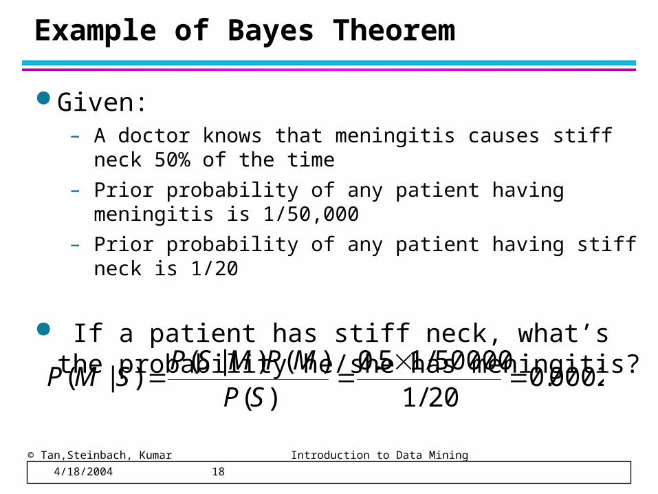
Example of Bayes Theorem
Given: – A doctor knows that meningitis causes stiff neck 50% of the
time
– Prior probability of any patient having meningitis is 1/50,000
– Prior probability of any patient having stiff neck is 1/20
If a patient has stiff neck, what’s the probability he/she has meningitis?
0002.020/150000/15.0
)()()|(
)|( SP
MPMSPSMP
© Tan,Steinbach, Kumar Introduction to Data Mining 4/18/2004 19
Bayesian Classifiers
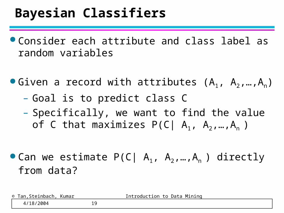
Consider each attribute and class label as random variables
Given a record with attributes (A1, A2,…,An)
– Goal is to predict class C
– Specifically, we want to find the value of C that maximizes P(C| A1, A2,…,An )
Can we estimate P(C| A1, A2,…,An ) directly from data?
© Tan,Steinbach, Kumar Introduction to Data Mining 4/18/2004 20
Bayesian Classifiers
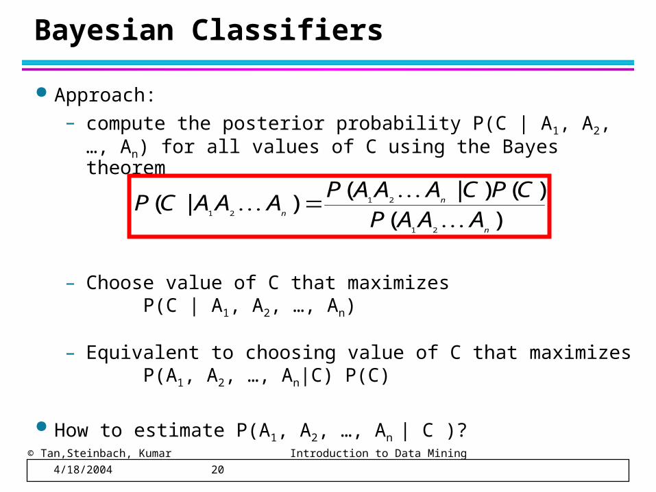
Approach:
– compute the posterior probability P(C | A1, A2, …, An) for all values of C using the Bayes theorem
– Choose value of C that maximizes P(C | A1, A2, …, An)
– Equivalent to choosing value of C that maximizes P(A1, A2, …, An|C) P(C)
How to estimate P(A1, A2, …, An | C )?
)()()|(
)|(21
21
21
n
n
n AAAPCPCAAAP
AAACP
© Tan,Steinbach, Kumar Introduction to Data Mining 4/18/2004 21
Naïve Bayes Classifier
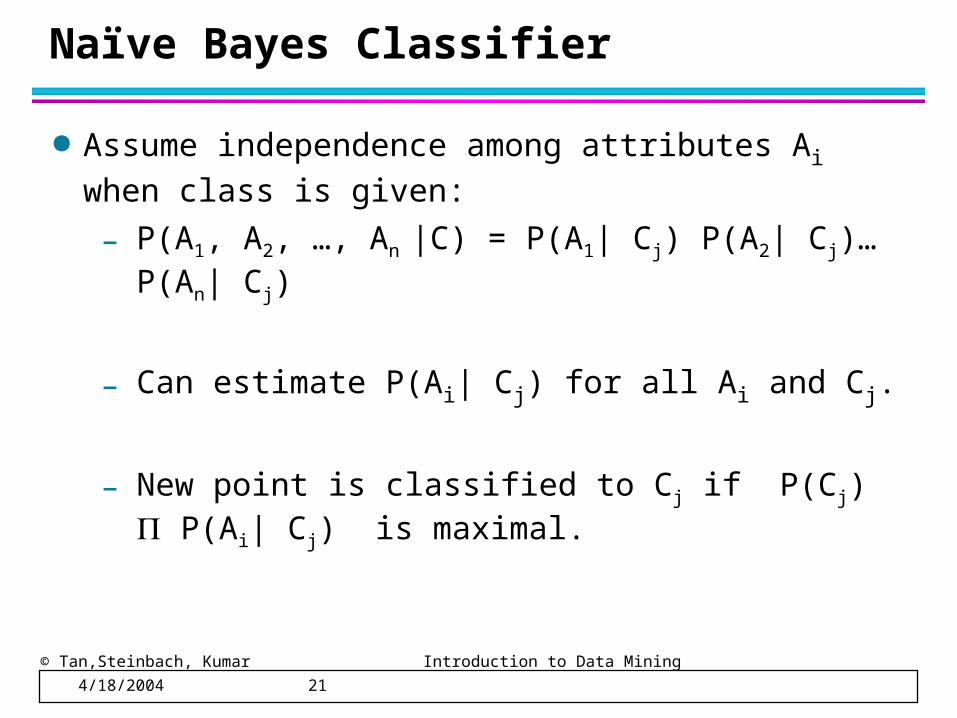
Assume independence among attributes Ai when class is
given:
– P(A1, A2, …, An |C) = P(A1| Cj) P(A2| Cj)… P(An| Cj)
– Can estimate P(Ai| Cj) for all Ai and Cj.
– New point is classified to Cj if P(Cj) P(Ai| Cj) is maximal.

© Tan,Steinbach, Kumar Introduction to Data Mining 4/18/2004 22
How to Estimate Probabilities from Data?
Class: P(C) = Nc/N– e.g., P(No) = 7/10,
P(Yes) = 3/10
For discrete attributes:
P(Ai | Ck) = |Aik|/ Nc
– where |Aik| is number of instances having attribute Ai and belongs to class Ck
– Examples:
P(Status=Married|No) = 4/7P(Refund=Yes|Yes)=0
k
© Tan,Steinbach, Kumar Introduction to Data Mining 4/18/2004 23
How to Estimate Probabilities from Data?
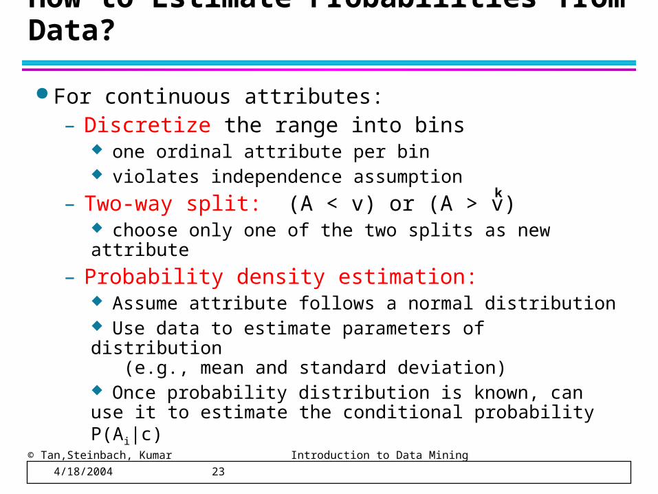
For continuous attributes: – Discretize the range into bins
one ordinal attribute per bin violates independence assumption
– Two-way split: (A < v) or (A > v) choose only one of the two splits as new attribute
– Probability density estimation: Assume attribute follows a normal distribution Use data to estimate parameters of distribution (e.g., mean and standard deviation) Once probability distribution is known, can use it to estimate the conditional probability P(Ai|c)
k
© Tan,Steinbach, Kumar Introduction to Data Mining 4/18/2004 24
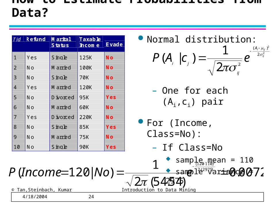
How to Estimate Probabilities from Data?
Normal distribution:
– One for each (Ai,ci) pair
For (Income, Class=No):
– If Class=No sample mean = 110 sample variance = 2975
2
2
2
)(
221
)|( ij
ijiA
ij
jiecAP
0072.0)54.54(2
1)|120( )2975(2
)110120( 2
eNoIncomeP
© Tan,Steinbach, Kumar Introduction to Data Mining 4/18/2004 25
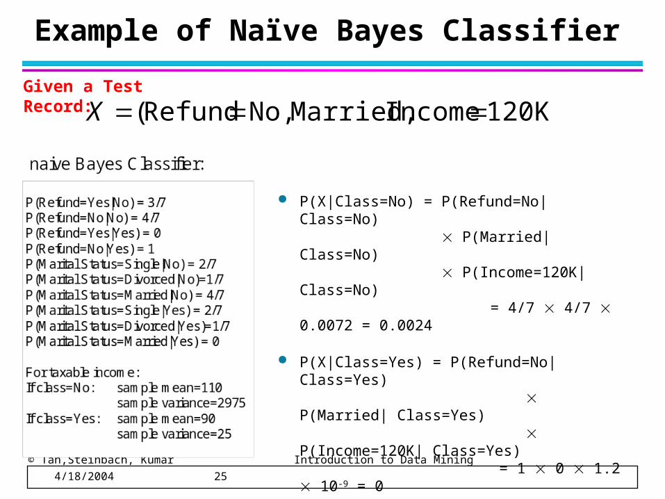
Example of Naïve Bayes Classifier
120K)IncomeMarried,No,Refund( X
P(X|Class=No) = P(Refund=No|Class=No) P(Married| Class=No) P(Income=120K|
Class=No) = 4/7 4/7 0.0072 = 0.0024
P(X|Class=Yes) = P(Refund=No| Class=Yes) P(Married| Class=Yes) P(Income=120K| Class=Yes)
= 1 0 1.2 10-9 = 0
Since P(X|No)P(No) > P(X|Yes)P(Yes)
Therefore P(No|X) > P(Yes|X) => Class = No
Given a Test Record:
© Tan,Steinbach, Kumar Introduction to Data Mining 4/18/2004 26
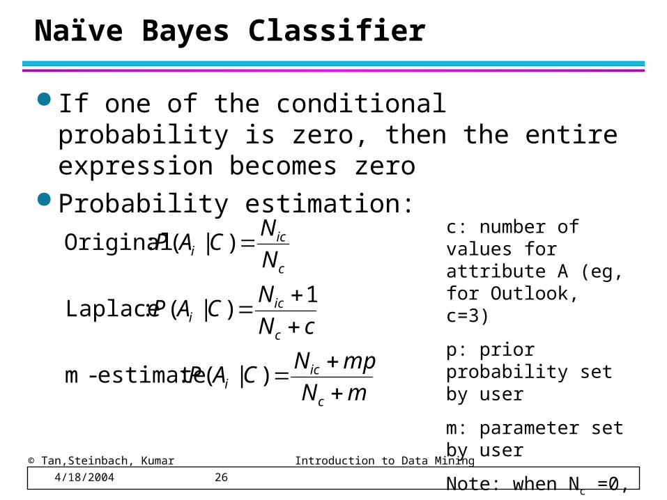
Naïve Bayes Classifier
If one of the conditional probability is zero, then the entire expression becomes zero
Probability estimation:
mN
mpNCAP
cN
NCAP
N
NCAP
c
ici
c
ici
c
ici
)|(:estimate-m
1)|(:Laplace
)|( :Originalc: number of values for attribute A (eg, for Outlook, c=3)
p: prior probability set by user
m: parameter set by user
Note: when Nc =0, P(Ai|C)=p.
© Tan,Steinbach, Kumar Introduction to Data Mining 4/18/2004 27
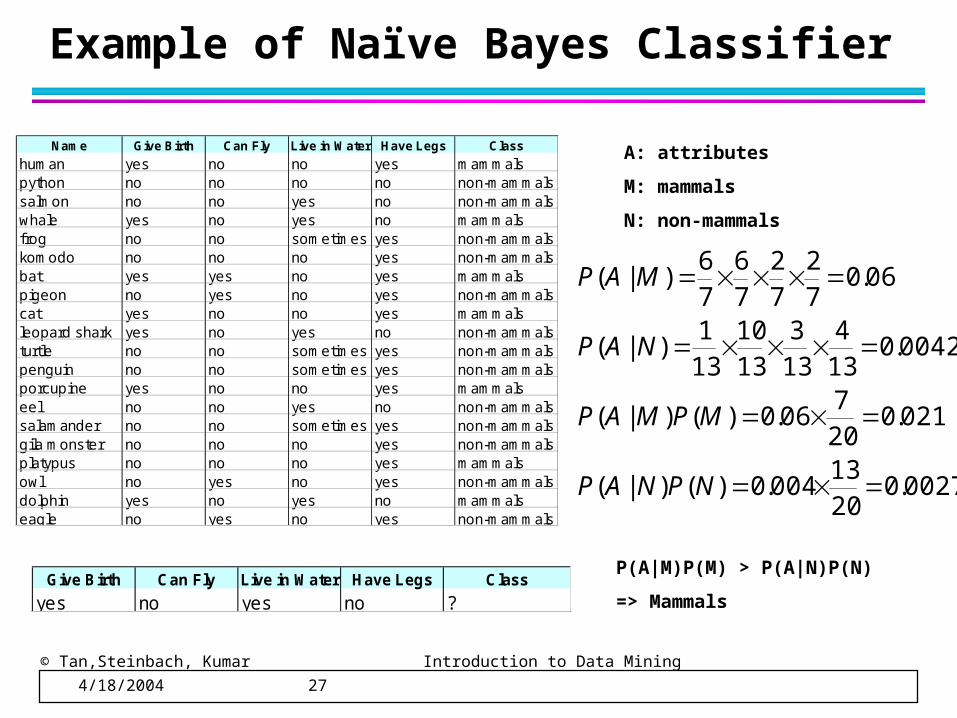
Example of Naïve Bayes Classifier
Name Give Birth Can Fly Live in Water Have Legs Class
human yes no no yes mammalspython no no no no non-mammalssalmon no no yes no non-mammalswhale yes no yes no mammalsfrog no no sometimes yes non-mammalskomodo no no no yes non-mammalsbat yes yes no yes mammalspigeon no yes no yes non-mammalscat yes no no yes mammalsleopard shark yes no yes no non-mammalsturtle no no sometimes yes non-mammalspenguin no no sometimes yes non-mammalsporcupine yes no no yes mammalseel no no yes no non-mammalssalamander no no sometimes yes non-mammalsgila monster no no no yes non-mammalsplatypus no no no yes mammalsowl no yes no yes non-mammalsdolphin yes no yes no mammalseagle no yes no yes non-mammals
Give Birth Can Fly Live in Water Have Legs Class
yes no yes no ?
0027.02013
004.0)()|(
021.0207
06.0)()|(
0042.0134
133
1310
131
)|(
06.072
72
76
76
)|(
NPNAP
MPMAP
NAP
MAP
A: attributes
M: mammals
N: non-mammals
P(A|M)P(M) > P(A|N)P(N)
=> Mammals

© Tan,Steinbach, Kumar Introduction to Data Mining 4/18/2004 28
Naïve Bayes (Summary)
Robust to isolated noise points
Handle missing values by ignoring the instance during probability estimate calculations
Robust to irrelevant attributes
Independence assumption may not hold for some attributes– Use other techniques such as Bayesian Belief
Networks (BBN)
© Tan,Steinbach, Kumar Introduction to Data Mining 4/18/2004 29
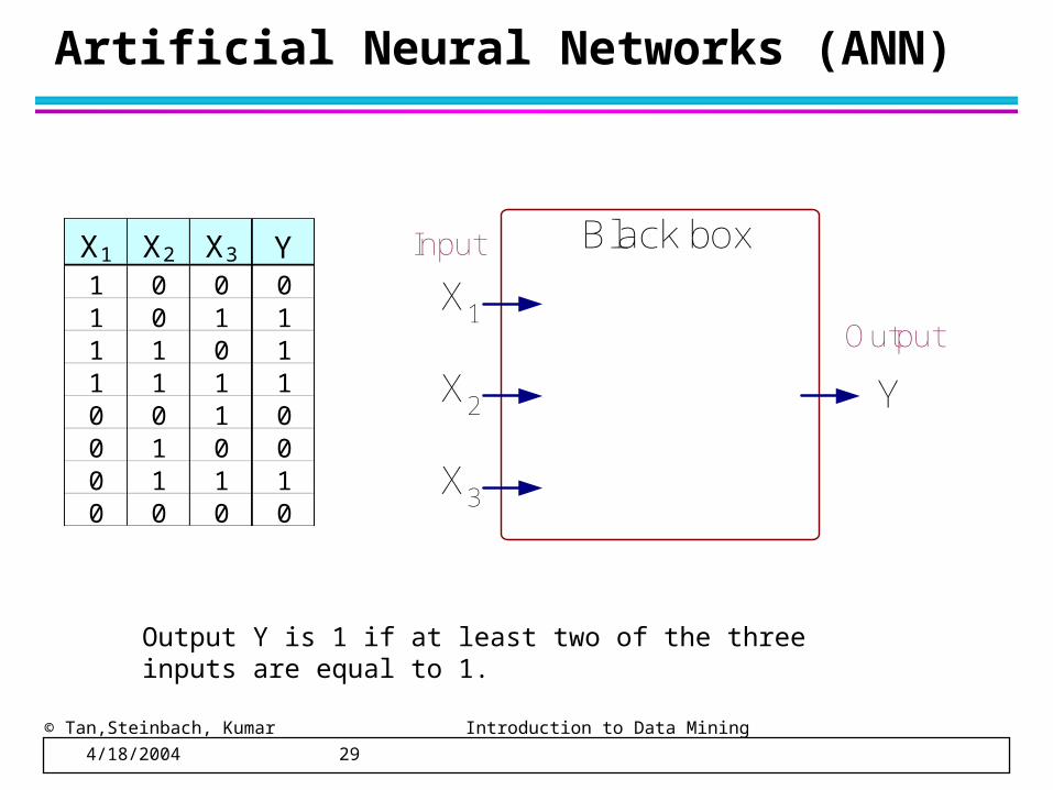
Artificial Neural Networks (ANN)
X1 X2 X3 Y1 0 0 01 0 1 11 1 0 11 1 1 10 0 1 00 1 0 00 1 1 10 0 0 0
X1
X2
X3
Y
Black box
Output
Input
Output Y is 1 if at least two of the three inputs are equal to 1.
© Tan,Steinbach, Kumar Introduction to Data Mining 4/18/2004 30
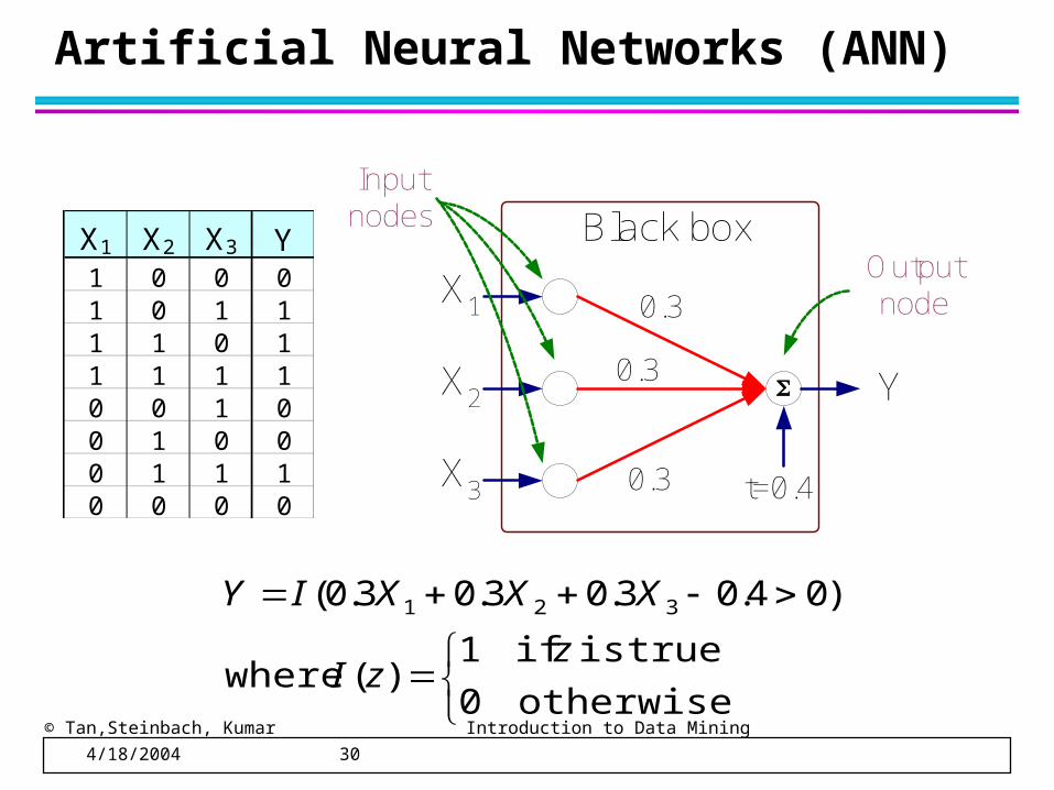
Artificial Neural Networks (ANN)
X1 X2 X3 Y1 0 0 01 0 1 11 1 0 11 1 1 10 0 1 00 1 0 00 1 1 10 0 0 0
X1
X2
X3
Y
Black box
0.3
0.3
0.3 t=0.4
Outputnode
Inputnodes
otherwise0
trueis if1)( where
)04.03.03.03.0( 321
zzI
XXXIY
© Tan,Steinbach, Kumar Introduction to Data Mining 4/18/2004 31
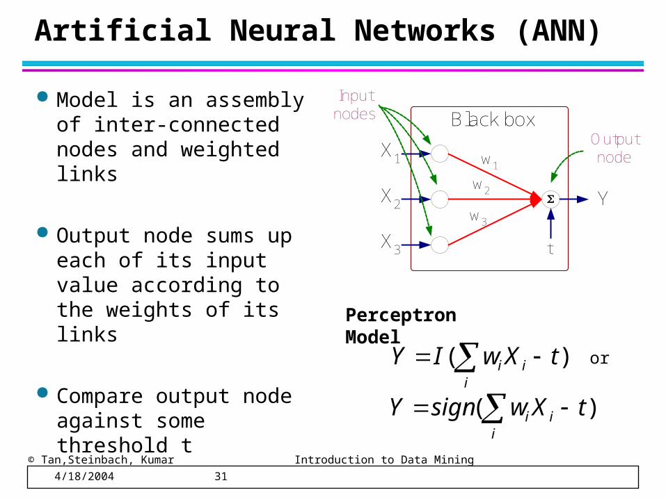
Artificial Neural Networks (ANN)
Model is an assembly of inter-connected nodes and weighted links
Output node sums up each of its input value according to the weights of its links
Compare output node against some threshold t
X1
X2
X3
Y
Black box
w1
t
Outputnode
Inputnodes
w2
w3
)( tXwIYi
ii Perceptron Model
)( tXwsignYi
ii
or
© Tan,Steinbach, Kumar Introduction to Data Mining 4/18/2004 32
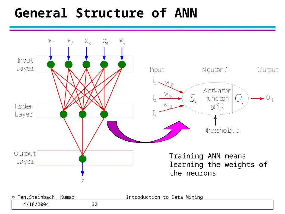
General Structure of ANN
Activationfunction
g(Si )Si Oi
I1
I2
I3
wi1
wi2
wi3
Oi
Neuron iInput Output
threshold, t
InputLayer
HiddenLayer
OutputLayer
x1 x2 x3 x4 x5
y
Training ANN means learning the weights of the neurons
© Tan,Steinbach, Kumar Introduction to Data Mining 4/18/2004 33
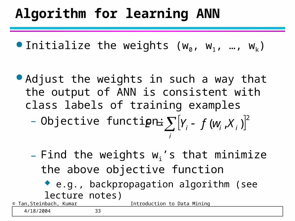
Algorithm for learning ANN
Initialize the weights (w0, w1, …, wk)
Adjust the weights in such a way that the output of ANN is consistent with class labels of training examples
– Objective function:
– Find the weights wi’s that minimize the above objective function e.g., backpropagation algorithm (see lecture notes)
2),( i
iii XwfYE
© Tan,Steinbach, Kumar Introduction to Data Mining 4/18/2004 34
More on Neural Networks: see additional notes
© Tan,Steinbach, Kumar Introduction to Data Mining 4/18/2004 35
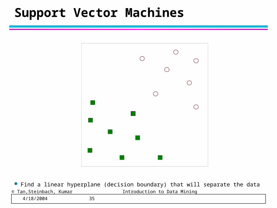
Support Vector Machines
Find a linear hyperplane (decision boundary) that will separate the data
© Tan,Steinbach, Kumar Introduction to Data Mining 4/18/2004 36
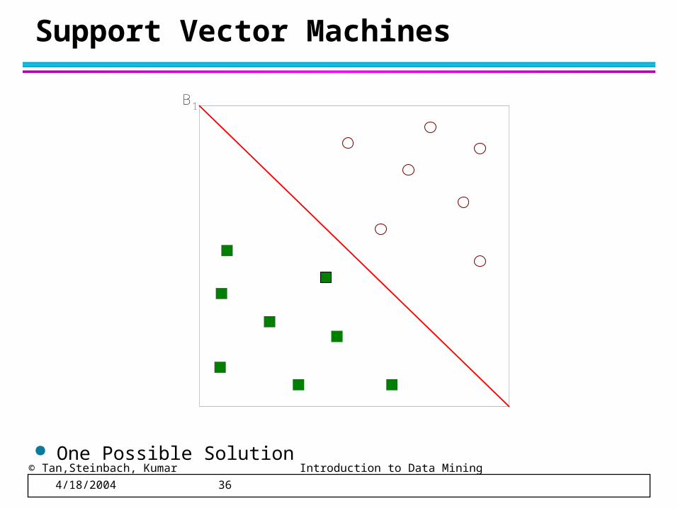
Support Vector Machines
One Possible Solution
B1

© Tan,Steinbach, Kumar Introduction to Data Mining 4/18/2004 37
Support Vector Machines
Another possible solution
B2
© Tan,Steinbach, Kumar Introduction to Data Mining 4/18/2004 38
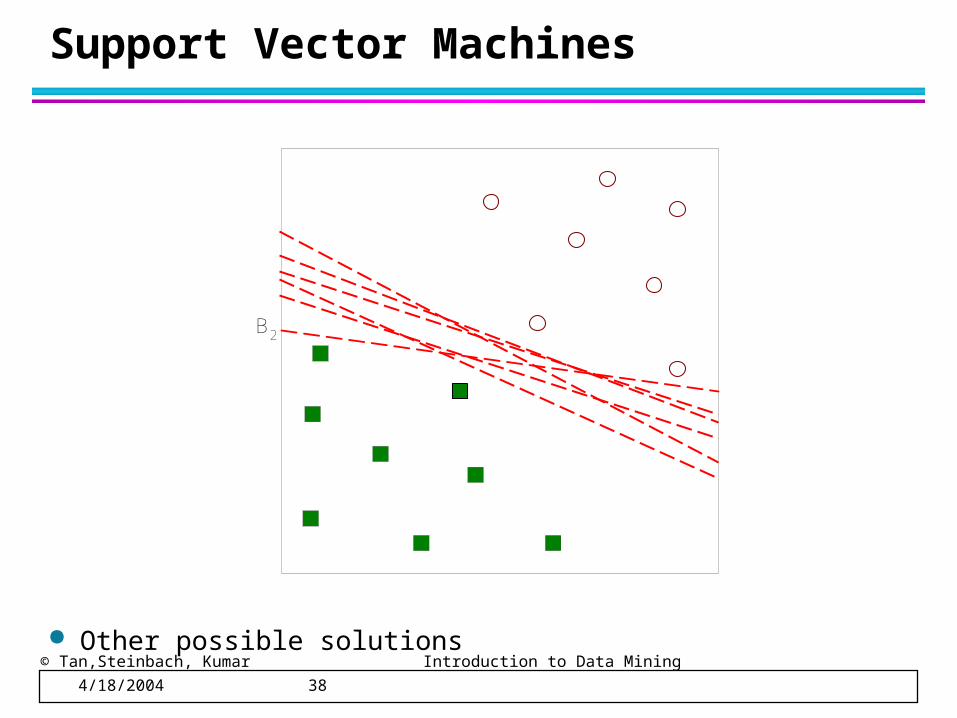
Support Vector Machines
Other possible solutions
B2
© Tan,Steinbach, Kumar Introduction to Data Mining 4/18/2004 39
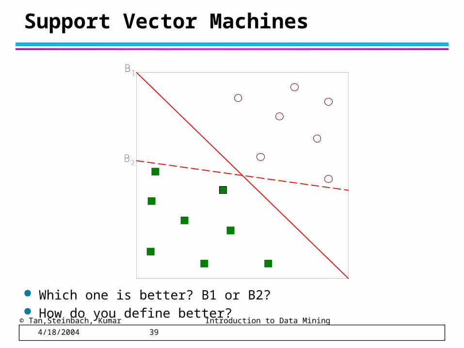
Support Vector Machines
Which one is better? B1 or B2? How do you define better?
B1
B2
© Tan,Steinbach, Kumar Introduction to Data Mining 4/18/2004 40
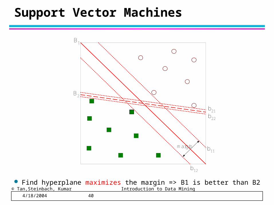
Support Vector Machines
Find hyperplane maximizes the margin => B1 is better than B2
B1
B2
b11
b12
b21
b22
margin
© Tan,Steinbach, Kumar Introduction to Data Mining 4/18/2004 41
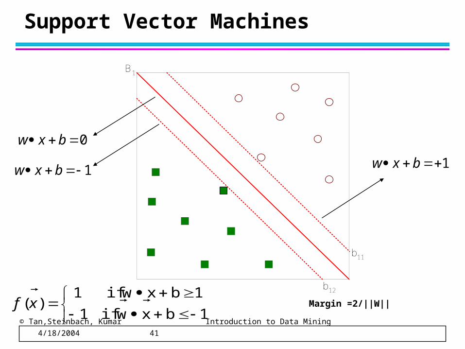
Support Vector Machines
B1
b11
b12
0 bxw
1 bxw 1 bxw
1bxw if1
1bxw if1)(
xf Margin =2/||W||
© Tan,Steinbach, Kumar Introduction to Data Mining 4/18/2004 42
Support Vector Machines
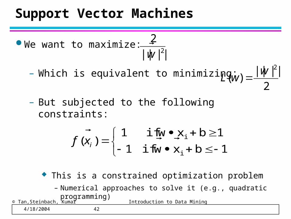
We want to maximize:
– Which is equivalent to minimizing:
– But subjected to the following constraints:
This is a constrained optimization problem– Numerical approaches to solve it (e.g., quadratic programming)
2||||
2
w
1bxw if1
1bxw if1)(
i
i
ixf
2
||||)(
2wwL
© Tan,Steinbach, Kumar Introduction to Data Mining 4/18/2004 43
Support Vector Machines
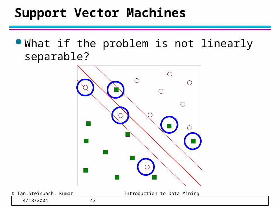
What if the problem is not linearly separable?
© Tan,Steinbach, Kumar Introduction to Data Mining 4/18/2004 44
Support Vector Machines
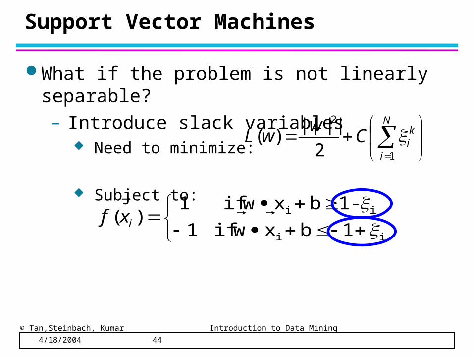
What if the problem is not linearly separable?
– Introduce slack variables Need to minimize:
Subject to:
ii
ii
1bxw if1
-1bxw if1)(
ixf
N
i
kiC
wwL
1
2
2
||||)(

© Tan,Steinbach, Kumar Introduction to Data Mining 4/18/2004 45
Nonlinear Support Vector Machines
What if decision boundary is not linear?
© Tan,Steinbach, Kumar Introduction to Data Mining 4/18/2004 46
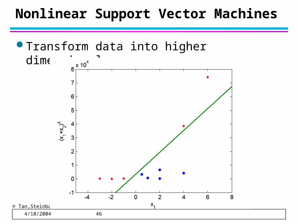
Nonlinear Support Vector Machines
Transform data into higher dimensional space
© Tan,Steinbach, Kumar Introduction to Data Mining 4/18/2004 47
Ensemble Methods:
Construct a set of classifiers from the training data
Predict class label of previously unseen records by aggregating predictions made by multiple classifiers
See additional Notes
Related Documents


![Chapter DM:II (continued) - webis.de · Cluster Evaluation [Tan/Steinbach/Kumar 2005] Random points DM:II-200 Cluster Analysis ©STEIN 2006-2019](https://static.cupdf.com/doc/110x72/5e0bb0aabeb12f5aad2f8024/chapter-dmii-continued-webisde-cluster-evaluation-tansteinbachkumar-2005.jpg)


