Data Mining

Data MiningPractical Machine Learning Tools and Techniques

Slides for Chapter 7 of Data Mining by I. H. Witten and E. Frank

2Data Mining: Practical Machine Learning Tools and Techniques (Chapter 7)

Engineering the input and output

� Attribute selection♦ Scheme-independent, scheme-specific

� Attribute discretization♦ Unsupervised, supervised, error- vs entropy-based, converse of discretization

� Data transformations♦ Principal component analysis, random projections, text, time series

� Dirty data♦ Data cleansing, robust regression, anomaly detection

� Meta-learning♦ Bagging (with costs), randomization, boosting, additive (logistic) regression,

option trees, logistic model trees, stacking, ECOCs

� Using unlabeled data♦ Clustering for classification, co-training, EM and co-training


Just apply a learner? NO!

� Scheme/parameter selectiontreat selection process as part of the learning

process� Modifying the input:

♦ Data engineering to make learning possible or easier

� Modifying the output♦ Combining models to improve performance


Attribute selection

� Adding a random (i.e. irrelevant) attribute can significantly degrade C4.5’s performance

♦ Problem: attribute selection based on smaller and smaller amounts of data

� IBL very susceptible to irrelevant attributes ♦ Number of training instances required increases

exponentially with number of irrelevant attributes

� Naïve Bayes doesn’t have this problem� Relevant attributes can also be harmful


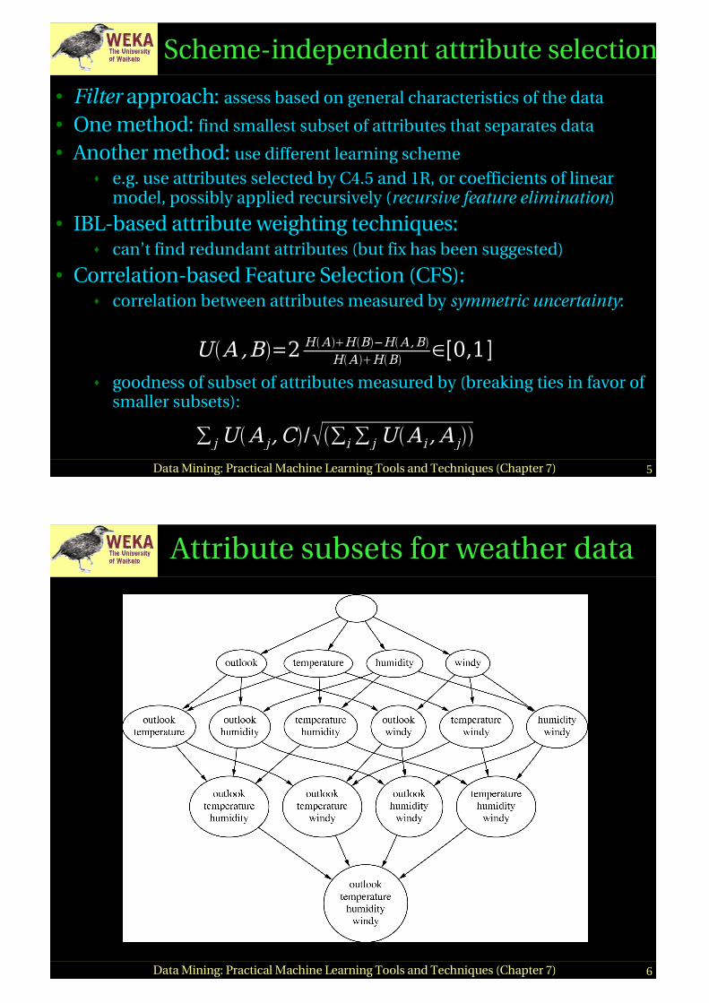
Scheme-independent attribute selection

� Filter approach: assess based on general characteristics of the data

� One method: find smallest subset of attributes that separates data

� Another method: use different learning scheme

♦ e.g. use attributes selected by C4.5 and 1R, or coefficients of linear model, possibly applied recursively (recursive feature elimination)

� IBL-based attribute weighting techniques:♦ can’t find redundant attributes (but fix has been suggested)

� Correlation-based Feature Selection (CFS):♦ correlation between attributes measured by symmetric uncertainty:

♦ goodness of subset of attributes measured by (breaking ties in favor of smaller subsets):

��

��

��


Attribute subsets for weather data


Searching attribute space

� Number of attribute subsets isexponential in number of attributes

� Common greedy approaches:� forward selection � backward elimination

� More sophisticated strategies:� Bidirectional search� Best-first search: can find optimum solution� Beam search: approximation to best-first search� Genetic algorithms


Scheme-specific selection� Wrapper approach to attribute selection� Implement “wrapper” around learning scheme

� Evaluation criterion: cross-validation performance

� Time consuming� greedy approach, k attributes ⇒ k2 × time

� prior ranking of attributes ⇒ linear in k

� Can use significance test to stop cross-validation for subset early if it is unlikely to “win” (race search)

� can be used with forward, backward selection, prior ranking, or special-purpose schemata search

� Learning decision tables: scheme-specific attribute selection essential

� Efficient for decision tables and Naïve Bayes


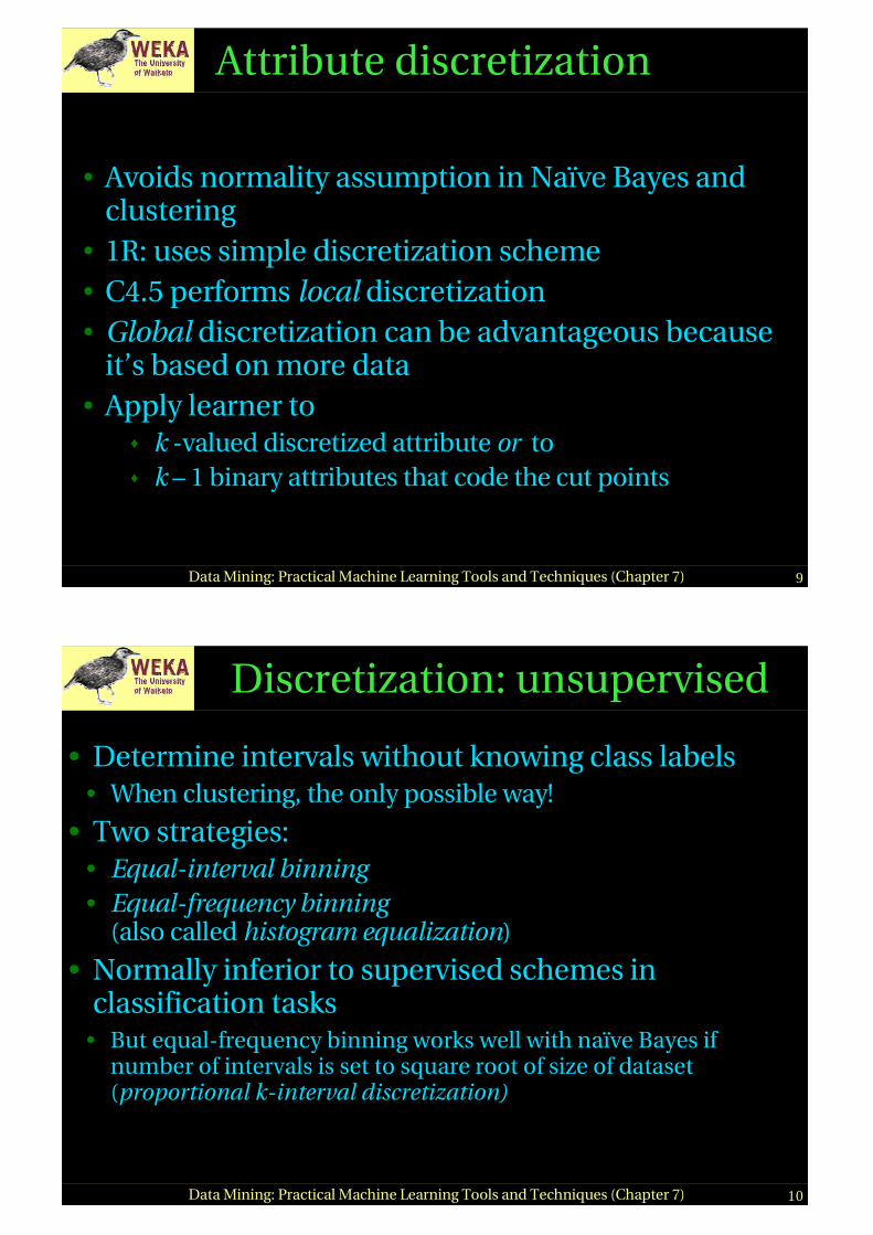
Attribute discretization

� Avoids normality assumption in Naïve Bayes and clustering

� 1R: uses simple discretization scheme� C4.5 performs local discretization� Global discretization can be advantageous because

it’s based on more data� Apply learner to

♦ k -valued discretized attribute or to♦ k – 1 binary attributes that code the cut points


Discretization: unsupervised

� Determine intervals without knowing class labels� When clustering, the only possible way!

� Two strategies:� Equal-interval binning� Equal-frequency binning

(also called histogram equalization)

� Normally inferior to supervised schemes in classification tasks

� But equal-frequency binning works well with naïve Bayes if number of intervals is set to square root of size of dataset (proportional k-interval discretization)


Discretization: supervised� Entropy-based method� Build a decision tree with pre-pruning on the

attribute being discretized� Use entropy as splitting criterion� Use minimum description length principle as stopping

criterion

� Works well: the state of the art� To apply min description length principle:

� The “theory” is� the splitting point (log2[N – 1] bits)

� plus class distribution in each subset

� Compare description lengths before/after adding split


Example: temperature attribute

Pl ay

Temper at ur e

Yes No Yes Yes Yes No No Yes Yes Yes No Yes Yes No

64 65 68 69 70 71 72 72 75 75 80 81 83 85


Formula for MDLP

� N instances� Original set: k classes, entropy E

� First subset: k1 classes, entropy E1

� Second subset: k2 classes, entropy E2

� Results in no discretization intervals for temperature attribute

� ��

��

��

�


Supervised discretization: other methods

� Can replace top-down procedure by bottom-up method

� Can replace MDLP by chi-squared test� Can use dynamic programming to find optimum

k-way split for given additive criterion♦ Requires time quadratic in the number of instances♦ But can be done in linear time if error rate is used

instead of entropy


Error-based vs. entropy-based

� Question:could the best discretization ever have two adjacent intervals with the same class?

� Wrong answer: No. For if so,� Collapse the two� Free up an interval� Use it somewhere else� (This is what error-based discretization will do)

� Right answer: Surprisingly, yes.� (and entropy-based discretization can do it)


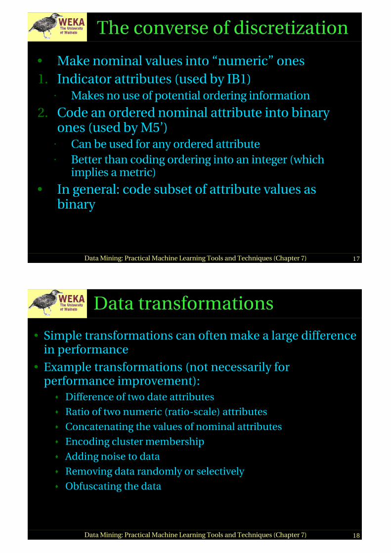
The converse of discretization

� Make nominal values into “numeric” ones

1. Indicator attributes (used by IB1)� Makes no use of potential ordering information

2. Code an ordered nominal attribute into binary ones (used by M5’)

� Can be used for any ordered attribute� Better than coding ordering into an integer (which

implies a metric)

� In general: code subset of attribute values as binary


Data transformations

� Simple transformations can often make a large difference in performance

� Example transformations (not necessarily for performance improvement):

♦ Difference of two date attributes

♦ Ratio of two numeric (ratio-scale) attributes

♦ Concatenating the values of nominal attributes

♦ Encoding cluster membership

♦ Adding noise to data

♦ Removing data randomly or selectively

♦ Obfuscating the data


Principal component analysis� Method for identifying the important “directions”

in the data� Can rotate data into (reduced) coordinate system

that is given by those directions� Algorithm:

1. Find direction (axis) of greatest variance

2. Find direction of greatest variance that is perpendicular to previous direction and repeat

� Implementation: find eigenvectors of covariance matrix by diagonalization

� Eigenvectors (sorted by eigenvalues) are the directions


Example: 10-dimensional data

� Can transform data into space given by components

� Data is normally standardized for PCA

� Could also apply this recursively in tree learner


Random projections

� PCA is nice but expensive: cubic in number of attributes

� Alternative: use random directions (projections) instead of principle components

� Surprising: random projections preserve distance relationships quite well (on average)

♦ Can use them to apply kD-trees to high-dimensional data

♦ Can improve stability by using ensemble of models based on different projections


Text to attribute vectors

� Many data mining applications involve textual data (eg. string attributes in ARFF)

� Standard transformation: convert string into bag of words by tokenization

♦ Attribute values are binary, word frequencies (fij),

log(1+fij), or TF × IDF:

� Only retain alphabetic sequences?

� What should be used as delimiters?

� Should words be converted to lowercase?

� Should stopwords be ignored?

� Should hapax legomena be included? Or even just the k most frequent words?

� � ��

��


Time series

� In time series data, each instance represents a different time step

� Some simple transformations:

♦ Shift values from the past/future

♦ Compute difference (delta) between instances (ie. “derivative”)

� In some datasets, samples are not regular but time is given by timestamp attribute

♦ Need to normalize by step size when transforming

� Transformations need to be adapted if attributes represent different time steps


Automatic data cleansing

� To improve a decision tree:♦ Remove misclassified instances, then re-learn!

� Better (of course!):♦ Human expert checks misclassified instances

� Attribute noise vs class noise♦ Attribute noise should be left in training set

(don’t train on clean set and test on dirty one)♦ Systematic class noise (e.g. one class substituted for

another): leave in training set♦ Unsystematic class noise: eliminate from training

set, if possible


Robust regression

� “Robust” statistical method ⇒ one that addresses problem of outliers

� To make regression more robust:� Minimize absolute error, not squared error� Remove outliers (e.g. 10% of points farthest from

the regression plane)� Minimize median instead of mean of squares

(copes with outliers in x and y direction)� Finds narrowest strip covering half the observations


Example: least median of squares

Number of international phone calls from Belgium, 1950–1973


Detecting anomalies

� Visualization can help to detect anomalies� Automatic approach:

committee of different learning schemes ♦ E.g.

� decision tree� nearest-neighbor learner� linear discriminant function

♦ Conservative approach: delete instances incorrectly classified by all of them

♦ Problem: might sacrifice instances of small classes


Combining multiple models

� Basic idea:build different “experts”, let them vote

� Advantage:♦ often improves predictive performance

� Disadvantage:♦ usually produces output that is very hard to

analyze

♦ but: there are approaches that aim to produce a single comprehensible structure


Bagging

� Combining predictions by voting/averaging� Simplest way� Each model receives equal weight

� “Idealized” version:� Sample several training sets of size n

(instead of just having one training set of size n)� Build a classifier for each training set� Combine the classifiers’ predictions

� Learning scheme is unstable ⇒ almost always improves performance

� Small change in training data can make big change in model (e.g. decision trees)


Bias-variance decomposition

� Used to analyze how much selection of any specific training set affects performance

� Assume infinitely many classifiers,built from different training sets of size n

� For any learning scheme,♦ Bias = expected error of the combined

classifier on new data♦ Variance= expected error due to the

particular training set used

� Total expected error ≈ bias + variance


More on bagging

� Bagging works because it reduces variance by voting/averaging

♦ Note: in some pathological hypothetical situations the overall error might increase

♦ Usually, the more classifiers the better

� Problem: we only have one dataset!� Solution: generate new ones of size n by sampling

from it with replacement � Can help a lot if data is noisy� Can also be applied to numeric prediction

♦ Aside: bias-variance decomposition originally only known for numeric prediction


Bagging classifiers

Let n be the number of instances in the training dataFor each of t iterations:

Sample n instances from training set( with replacement)

Apply learning algorithm to the sampleStore resulting model

For each of the t models:Predict class of instance using model

Return class that is predicted most often

Model generation

Classification


Bagging with costs

� Bagging unpruned decision trees known to produce good probability estimates

♦ Where, instead of voting, the individual classifiers' probability estimates are averaged

♦ Note: this can also improve the success rate

� Can use this with minimum-expected cost approach for learning problems with costs

� Problem: not interpretable♦ MetaCost re-labels training data using bagging with

costs and then builds single tree


Randomization

� Can randomize learning algorithm instead of input

� Some algorithms already have a random component: eg. initial weights in neural net

� Most algorithms can be randomized, eg. greedy algorithms:

♦ Pick from the N best options at random instead of always picking the best options

♦ Eg.: attribute selection in decision trees

� More generally applicable than bagging: e.g. random subsets in nearest-neighbor scheme

� Can be combined with bagging


Boosting

� Also uses voting/averaging� Weights models according to performance� Iterative: new models are influenced by

performance of previously built ones♦ Encourage new model to become an “expert”

for instances misclassified by earlier models♦ Intuitive justification: models should be

experts that complement each other

� Several variants


AdaBoost.M1

Assign equal weight to each training instanceFor t iterations: Apply learning algorithm to weighted dataset,

store resulting model Compute model’s error e on weighted dataset If e = 0 or e ≥ 0.5: Terminate model generation For each instance in dataset: If classified correctly by model: Multiply instance’s weight by e/(1- e) Normalize weight of all instances

Model generation

ClassificationAssign weight = 0 to all classesFor each of the t (or less) models:

For the class this model predictsadd –log e/(1- e) to this class’s weight

Return class with highest weight


More on boosting I� Boosting needs weights … but� Can adapt learning algorithm ... or� Can apply boosting without weights

� resample with probability determined by weights� disadvantage: not all instances are used� advantage: if error > 0.5, can resample again

� Stems from computational learning theory� Theoretical result:

� training error decreases exponentially

� Also:� works if base classifiers are not too complex, and� their error doesn’t become too large too quickly


More on boosting II� Continue boosting after training error = 0?� Puzzling fact:

generalization error continues to decrease!� Seems to contradict Occam’s Razor

� Explanation:consider margin (confidence), not error

� Difference between estimated probability for true class and nearest other class (between –1 and 1)

� Boosting works with weak learnersonly condition: error doesn’t exceed 0.5

� In practice, boosting sometimes overfits (in contrast to bagging)


Additive regression I

� Turns out that boosting is a greedy algorithm for fitting additive models

� More specifically, implements forward stagewise additive modeling

� Same kind of algorithm for numeric prediction:

1.Build standard regression model (eg. tree)

2.Gather residuals, learn model predicting residuals (eg. tree), and repeat

� To predict, simply sum up individual predictions from all models


Additive regression II

� Minimizes squared error of ensemble if base learner minimizes squared error

� Doesn't make sense to use it with standard multiple linear regression, why?

� Can use it with simple linear regression to build multiple linear regression model

� Use cross-validation to decide when to stop

� Another trick: shrink predictions of the base models by multiplying with pos. constant < 1

♦ Caveat: need to start with model 0 that predicts the mean


Additive logistic regression

� Can use the logit transformation to get algorithm for classification

♦ More precisely, class probability estimation

♦ Probability estimation problem is transformed into regression problem

♦ Regression scheme is used as base learner (eg. regression tree learner)

� Can use forward stagewise algorithm: at each stage, add model that maximizes probability of data

� If fj is the jth regression model, the ensemble predicts

probability for the first class !��"� ��

��#! ��


LogitBoost

� Maximizes probability if base learner minimizes squared error

� Difference to AdaBoost: optimizes probability/likelihood instead of exponential loss

� Can be adapted to multi-class problems

� Shrinking and cross-validation-based selection apply

For j = 1 to t iterations: For each instance a[i]: Set the target value for the regression to z[i] = (y[i] – p(1|a[i])) / [p(1|a[i]) × (1-p(1|a[i])] Set the weight of instance a[i] to p(1|a[i]) × (1-p(1|a[i]) Fit a regression model f[j] to the data with class values z[i] and weights w[i]

Model generation

Classification

Predict 1 st class if p(1 | a) > 0.5, otherwise predict 2 nd class


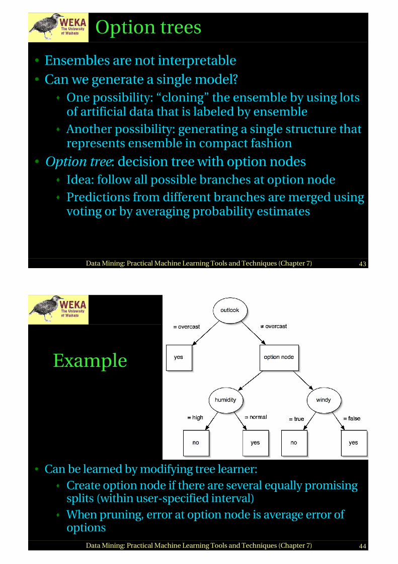
Option trees

� Ensembles are not interpretable� Can we generate a single model?

♦ One possibility: “cloning” the ensemble by using lots of artificial data that is labeled by ensemble

♦ Another possibility: generating a single structure that represents ensemble in compact fashion

� Option tree: decision tree with option nodes♦ Idea: follow all possible branches at option node

♦ Predictions from different branches are merged using voting or by averaging probability estimates


Example

� Can be learned by modifying tree learner:

♦ Create option node if there are several equally promising splits (within user-specified interval)

♦ When pruning, error at option node is average error of options


Alternating decision trees

� Can also grow option tree by incrementally adding nodes to it

� Structure called alternating decision tree, with splitter nodes and prediction nodes

♦ Prediction nodes are leaves if no splitter nodes have been added to them yet

♦ Standard alternating tree applies to 2-class problems

♦ To obtain prediction, filter instance down all applicable branches and sum predictions

� Predict one class or the other depending on whether the sum is positive or negative


Example


Growing alternating trees� Tree is grown using a boosting algorithm

♦ Eg. LogitBoost described earlier

♦ Assume that base learner produces single conjunctive rule in each boosting iteration (note: rule for regression)

♦ Each rule could simply be added into the tree, including the numeric prediction obtained from the rule

♦ Problem: tree would grow very large very quickly

♦ Solution: base learner should only consider candidate rules that extend existing branches

� Extension adds splitter node and two prediction nodes (assuming binary splits)

♦ Standard algorithm chooses best extension among all possible extensions applicable to tree

♦ More efficient heuristics can be employed instead


Logistic model trees

� Option trees may still be difficult to interpret

� Can also use boosting to build decision trees with linear models at the leaves (ie. trees without options)

� Algorithm for building logistic model trees:♦ Run LogitBoost with simple linear regression as base learner

(choosing the best attribute in each iteration)

♦ Interrupt boosting when cross-validated performance of additive model no longer increases

♦ Split data (eg. as in C4.5) and resume boosting in subsets of data

♦ Prune tree using cross-validation-based pruning strategy (from CART tree learner)


Stacking

� To combine predictions of base learners, don’t vote, use meta learner

♦ Base learners: level-0 models♦ Meta learner: level-1 model♦ Predictions of base learners are input to meta learner

� Base learners are usually different schemes� Can’t use predictions on training data to generate

data for level-1 model!♦ Instead use cross-validation-like scheme

� Hard to analyze theoretically: “black magic”


More on stacking

� If base learners can output probabilities, use those as input to meta learner instead

� Which algorithm to use for meta learner?♦ In principle, any learning scheme♦ Prefer “relatively global, smooth” model

� Base learners do most of the work� Reduces risk of overfitting

� Stacking can be applied to numeric prediction too


Error-correcting output codes

� Multiclass problem ⇒ binary problems� Simple scheme:

One-per-class coding

� Idea: use error-correcting codes instead

� base classifiers predict1011111, true class = ??

� Use code words that havelarge Hamming distancebetween any pair

� Can correct up to (d – 1)/2 single-bit errors

0001d

0010c

0100b

1000a

class vectorclass

0101010d

0011001c

0000111b

1111111a

class vectorclass


More on ECOCs

� Two criteria :� Row separation:

minimum distance between rows� Column separation:

minimum distance between columns� (and columns’ complements)� Why? Because if columns are identical, base classifiers will likely

make the same errors� Error-correction is weakened if errors are correlated

� 3 classes ⇒ only 23 possible columns � (and 4 out of the 8 are complements)� Cannot achieve row and column separation

� Only works for problems with > 3 classes


Exhaustive ECOCs

� Exhaustive code for k classes:� Columns comprise every

possible k-string …� … except for complements

and all-zero/one strings� Each code word contains

2k–1 – 1 bits

� Class 1: code word is all ones� Class 2: 2k–2 zeroes followed by 2k–2 –1 ones� Class i : alternating runs of 2k–i 0s and 1s

� last run is one short

0101010d

0011001c

0000111b

1111111a

class vectorclass

Exhaustive code, k = 4


More on ECOCs

� More classes ⇒ exhaustive codes infeasible� Number of columns increases exponentially

� Random code words have good error-correcting properties on average!

� There are sophisticated methods for generating ECOCs with just a few columns

� ECOCs don’t work with NN classifier� But: works if different attribute subsets are used to predict

each output bit


Using unlabeled data

� Semisupervised learning: attempts to use unlabeled data as well as labeled data

♦ The aim is to improve classification performance

� Why try to do this? Unlabeled data is often plentiful and labeling data can be expensive

♦ Web mining: classifying web pages

♦ Text mining: identifying names in text

♦ Video mining: classifying people in the news

� Leveraging the large pool of unlabeled examples would be very attractive


Clustering for classification

� Idea: use naïve Bayes on labeled examples and then apply EM

♦ First, build naïve Bayes model on labeled data

♦ Second, label unlabeled data based on class probabilities (“expectation” step)

♦ Third, train new naïve Bayes model based on all the data (“maximization” step)

♦ Fourth, repeat 2nd and 3rd step until convergence

� Essentially the same as EM for clustering with fixed cluster membership probabilities for labeled data and #clusters = #classes


Comments

� Has been applied successfully to document classification

♦ Certain phrases are indicative of classes

♦ Some of these phrases occur only in the unlabeled data, some in both sets

♦ EM can generalize the model by taking advantage of co-occurrence of these phrases

� Refinement 1: reduce weight of unlabeled data � Refinement 2: allow multiple clusters per class


Co-training

� Method for learning from multiple views (multiple sets of attributes), eg:

♦ First set of attributes describes content of web page

♦ Second set of attributes describes links that link to the web page

� Step 1: build model from each view� Step 2: use models to assign labels to unlabeled data� Step 3: select those unlabeled examples that were most

confidently predicted (ideally, preserving ratio of classes)� Step 4: add those examples to the training set� Step 5: go to Step 1 until data exhausted� Assumption: views are independent


EM and co-training

� Like EM for semisupervised learning, but view is switched in each iteration of EM

♦ Uses all the unlabeled data (probabilistically labeled) for training

� Has also been used successfully with support vector machines

♦ Using logistic models fit to output of SVMs

� Co-training also seems to work when views are chosen randomly!

♦ Why? Possibly because co-trained classifier is more robust

Data Mining

Documents

techniques chapter

learning possible

attributes linear

different learning scheme

problemrelevant attributes

redundant attributes

attribute selectionadding

smallest subset of attributes